The Signaling Value of a High School Diplomafaculty.smu.edu/millimet/classes/eco7321/papers/clark...

The Signaling Value of a High School DiplomaAuthor(s): Damon Clark and Paco MartorellSource: Journal of Political Economy, Vol. 122, No. 2 (April 2014), pp. 282-318Published by: The University of Chicago PressStable URL: http://www.jstor.org/stable/10.1086/675238 .

Accessed: 16/05/2014 11:20

Your use of the JSTOR archive indicates your acceptance of the Terms & Conditions of Use, available at .http://www.jstor.org/page/info/about/policies/terms.jsp

.JSTOR is a not-for-profit service that helps scholars, researchers, and students discover, use, and build upon a wide range ofcontent in a trusted digital archive. We use information technology and tools to increase productivity and facilitate new formsof scholarship. For more information about JSTOR, please contact [email protected].

.

The University of Chicago Press is collaborating with JSTOR to digitize, preserve and extend access to Journalof Political Economy.

http://www.jstor.org

This content downloaded from 129.119.38.195 on Fri, 16 May 2014 11:20:18 AMAll use subject to JSTOR Terms and Conditions

http://www.jstor.org/action/showPublisher?publisherCode=ucpress

http://www.jstor.org/stable/10.1086/675238?origin=JSTOR-pdf

http://www.jstor.org/page/info/about/policies/terms.jsp


The Signaling Value of a High School Diploma

Damon Clark

University of California, Irvine, and National Bureau of Economic Research

Paco Martorell

RAND

This paper distinguishes between the human capital and signaling the-ories by estimating the earnings return to a high school diploma. Un-

Weimprocordacommversitdon SRANDand Sthe Nforniawas viMarioouslyNatio01Þ. Tthe Tpartm

[ Journa© 2014

like most indicators of education ðe.g., a year of schoolÞ, a diploma isessentially a piece of paper and, hence, by itself cannot affect productiv-ity. Any earnings return to holding a diploma must therefore reflect thediploma’s signaling value. Using regression discontinuity methods tocompare the earnings of workers who barely passed and barely failedhigh school exit exams—standardized tests that students must pass toearn a high school diploma—we find little evidence of diploma signal-ing effects.

thank the editor and anonymous referee for suggestions and comments that greatlyved the paper. For useful discussions, we thank Ken Chay, Mike Geruso, Marco Mana-, Rob McMillan, Devah Pager, Craig Riddell, and, especially, David Lee. For helpfulents and suggestions, we thank seminar participants at Bristol University, Brown Uni-y, Columbia University, the Florida Department of Education, Harvard University, Lon-chool of Economics, Northwestern University, Pompeu Fabra, Princeton University,, Rutgers University, University of Toronto, University of California at Davis, Irvine,anta Barbara, University of Florida, the Society of Labor Economists 2010 conference,ational Bureau of Economic Research 2010 Summer Institute, and the Southern Cali-Conference of AppliedMicroeconomics.Much of this work was completedwhile Clarksiting the Industrial Relations Section at PrincetonUniversity.We thankLaurelWheeler,n Aouad, and Yu Xue for excellent research assistance. Financial support was gener-provided by the US Department of Education ðunder grant R305R060096Þ and thenal Institute of Child Health and Human Development ðunder grant R01HD054637-he opinions expressed in this paper are ours and do not necessarily reflect the views ofexas Education Agency, the Texas Higher Education Coordinating Board, the US De-ent of Education, or the National Institute of Child Health and Human Development.

l of Political Economy, 2014, vol. 122, no. 2]by The University of Chicago. All rights reserved. 0022-3808/2014/12202-0004$10.00

282



I. Introduction

signaling value of a high school diploma 283

According to the theory of human capital, individuals invest in educationto increase their productivity and, therefore, their wages ðBecker 1964Þ.Human capital theory has been used to explain the life cycle profile ofwages ðMincer 1974Þ and the distribution of wages ðBecker 1967Þ. It alsounderpins explanations for wage and productivity differences across cit-ies ðMoretti 2010Þ and for differences in the level and growth of produc-tivity across countries ðLucas 1988; Romer 1990Þ. Signaling theory pro-vides an alternative rationale for educational investments. According tosignaling theory, firms have imperfect information about worker pro-ductivity, and individuals invest in education to signal their productivityto firms and thereby increase their wages ðSpence 1973Þ. If signaling the-ory is important, it undermines explanations for economic phenomenabased on human capital theory. It also implies that the social returns toeducation could be lower than the private returns to education. Since thisimplication contrasts with recent research suggesting that the social re-turns to education might be higher than the private returns to education,it has important policy implications ðMoretti 2006Þ.The signaling and human capital theories are difficult to differentiate

empirically, and this has made it hard to determine the practical impor-tance of education-based signaling.1 The basic problem is that both the-ories imply that there will be a positive effect of education on wages. Thereason is that most types of education ðe.g., years of schooling, schoolqualityÞ could increase wages by improving productivity or by acting asproductivity signals.This paper aims to distinguish between the human capital and signal-

ing theories by estimating the signaling value of a high school diploma.There are two reasons why a high school diploma is an interesting cre-dential to analyze. First, it is the most commonly held credential in theUnited States.2 Second, unlike other indicators of education such as years

1
Previous approaches to distinguishing these theories have tested whether the privatereturns to education exceed the social returns to education ðas they would if signalingdominated any positive externalities associated with educationÞ, whether education policychanges affect the educational decisions of students they do not directly affect ðas theywould if those students wished to differentiate themselves from the directly affected stu-dentsÞ, and whether wage equations fit better for workers in occupations in which pro-ductivity cannot be observed ðas they would if productivity expectations and hence wagesin those occupations were based on signals such as educationÞ. See Lange and Topel ð2006Þfor a review and critique of the relevant papers.
2 In 2009, among individuals in the United States aged 25 and older, the highest degreeattained is an associate’s or higher for 39 percent, a high school diploma for 44 percent,and less than a high school diploma for 13 percent. The most common educational attain-ment categories are high school diploma ð31 percentÞ and 4-year college degree ð19 per-centÞ. These figures are authors’ calculations based on census tabulations from http://www.census.gov/population/www/socdemo/education/cps2009.html.



of schooling, it cannot affect productivity because it is essentially only apiece of paper, despite the strong correlation between productivity and

284 journal of political economy

diploma receipt, precisely the reason why it could act as a productivitysignal.3 This implies that we could, conceivably, estimate the signalingvalue of a diploma by randomly assigning it among a small group of work-ers. By virtue of the random assignment, the signaling value of the di-ploma would be captured by the earnings advantage enjoyed by the work-ers randomly assigned to receive it. Of course, in the broader population,the measured earnings advantage enjoyed by workers with diplomas re-flects this signaling value plus any productivity differences that firms ob-serve.4

To mimic the random assignment of diplomas, we use high schoolexit exams, tests that students must pass in order to graduate from highschool. These were first used in the 1980s and are now used in aroundhalf of US states.5 Typically, students in these states are first administeredthese exams in grade 10 or 11; those who fail can retake them in grades11 and 12. We focus on individuals who retook the exam at the end ofgrade 12 and compare those who barely passed and barely failed. Barelypassers are much more likely to receive a diploma since retaking optionsare limited for students who fail at this stage. Barely passers and barelyfailers should, however, be similar in all other dimensions that matterfor productivity since, under certain conditions ðLee 2008Þ, passing statuscan be viewed as effectively randomly assigned for individuals with scoresclose to the passing cutoff. This implies that an estimate of the signalingvalue of a diploma can be based on the earnings differences betweenthese two groups. We exploit this insight by applying fuzzy regression dis-continuity methods ðHahn, Todd, and van der Klaauw 2001Þ to a large ad-ministrative data set that links individual-level high school records to infor-mation on postsecondary schooling and earnings for up to 11 years afterhigh school graduation.Our findings suggest that a high school diploma has little signaling

value. Across a variety of specifications, the estimated diploma signalingvalues are close to zero and statistically insignificant. We obtain similar

3 We find in our data that among workers who completed grade 12 and did not attend
college, the diploma earnings differential—which will reflect the diploma productivitydifferential—is between 10 and 20 percent. Similar wage differentials are found in a varietyof other data sets ðe.g., Heckman and LaFontaine 2006Þ.
4 We are assuming that firms do not know which workers are in the experimental groupin which diploma status is randomly assigned.

5 By 2012, 26 states ðcontaining 76 percent of high school studentsÞ had high school exitexams ðZabala et al. 2007Þ. These exams were designed to create incentives to improvestudent achievement and to increase the value of a high school diploma. They are, how-ever, controversial because of concerns that they hurt students from disadvantaged back-grounds ðPeterson 2005Þ. Dee and Jacob ð2007Þ summarize the recent literature on exitexams.



results when we split the sample by sex and race and when we examinethe time profile of signaling values. We also obtain similar results when


we generate parallel estimates for another state (Florida) that operatesa similar exit exam policy (see the online Appendix for details). Since ahigh school diploma could signal both high school completion ði.e.,perseveranceÞ and passing the exam ði.e., cognitive skillsÞ, we interpretour results as evidence that, at least among our sample of twelfth-gradeexit exam retakers, neither high school completion nor high school di-ploma receipt is used to signal either cognitive or noncognitive skills.6

This finding cannot be explained by high school diplomas being unre-lated to productivity. Indeed, we find a strong correlation between di-ploma status and earnings both in our analysis sample consisting oftwelfth-grade exit exam retakers and more generally among those whocompleted twelfth grade and did not go to college.These findings differ from those obtained by previous studies, several

of which estimate that high school diplomas and completion of twelfthgrade are associated with large wage increases ðHungerford and Solon1987; Jaeger and Page 1996; Park 1999; Frazis 2002Þ. We argue that theseearlier studies did not adequately control for observable ðto firms but notto the econometricianÞ productivity differences between workers with andwithout these credentials.7

We conclude that our results provide a strong challenge to those whocontend that employers use high school completion and high school di-plomas to make inferences about unobserved productivity.

II. Institutional Setting

This section describes the key features of the relevant institutions. First,we briefly describe how exit exams operate in Texas, the site for our studyðthe Appendix provides a more detailed descriptionÞ. We then describe

6 This statement assumes that workers are not able to signal high school completionindependently of high school graduation. In principle, workers without a diploma could
inform employers that they completed high school. However, as we explain below, sincemost students in our sample did not have a mechanism for signaling completion inde-pendently of graduation ðe.g., via a certificate of completionÞ and since employers findit difficult to obtain grade information from schools ðe.g., Bishop 1988Þ, presenting em-ployers with a diploma is likely to be the easiest and most convenient way for students toconvey both high school graduation and completion of twelfth grade.
7 Our results also differ from those reported in Tyler, Murnane, and Willett ð2000Þ, whoused a difference-in-difference approach to estimating the return to a General EducationalDevelopment ðGEDÞ certificate, a credential that is typically pursued by high school drop-outs that is intended to be equivalent to a high school diploma ðHeckman, Humphries, andMader 2010Þ. Although they estimate large returns for some types of workers ðbetween 10and 20 percentÞ, Jepsen, Mueser, and Troske ð2010Þ argue that some of these estimates maybe influenced by selective retaking of the GED exams. They findmuch smaller GED returns,as do some other studies, including Cameron and Heckman ð1993Þ and Heckman andLaFontaine ð2006Þ.



exactly what the high school diploma represents and how diploma in-formation can be conveyed to employers.


A. High School Exit Exams in Texas

In order to earn a high school diploma in Texas, students must take andpass the minimum required courses set by state law. Aside from a rela-tively small number of students who receive special education waivers,students must also pass a standardized test known as a high school exitexam.8 In Texas, the exit exam includes math, reading, and writing sec-tions, and students without special education waivers must pass all threesections in order to graduate.Students first take the exit exam in the spring of tenth grade or the fall

of eleventh grade ðthis varies across cohorts during our study periodÞ.Following the initial attempt, there are retests administered periodicallyfor students who failed. On the day of a retest administration, studentswho have not passed all sections of the exam are required to retake theunpassed sections.9 Students can retake the exam after the end of twelfthgrade ðe.g., in the summer following twelfth grade or by returning toschool for a thirteenth gradeÞ. However, doing so is relatively uncom-mon, as shown below by the strong relationship between the outcome ofthe final retest given in twelfth grade and eventual high school diplomastatus.

B. High School Diplomas in Texas

We refer throughout to high school diplomas. Technically, however, stu-dents who graduate from high school earn a high school degree. Ac-cording to Texas state law, the official indicator that a student earned ahigh school degree is a high school graduation seal ðwhich is commonthroughout the stateÞ on a student’s high school transcript. The tran-script—which has to conform to guidelines set by the state—includes in-formation on courses completed, grades awarded, and the dates on whichthe exit exams were passed ðif they wereÞ. Appendix figure A1 shows asample Texas high school transcript.10 Typically, students also receive paperdiplomas at a school’s commencement ceremony. While these diplomas

8 In Texas during our study period, about 7 percent of high school students who reached
tenth grade received exemptions for some portion of the exit exam ðMartorell 2005Þ.
9 Retests are administered once in the fall, spring, and summer of each year. There isalso a retest given late in the spring for twelfth graders who have not yet passed the exam.In practice, students may not retake the exit exam if they are absent on the day the retestsare administered or if they have already dropped out of school. Retaking is also much lesscommon for the summer retest administrations, presumably because students do not at-tend school during the summer.

10 This form and other information about high school transcripts can be found athttp://www.tea.state.tx.us/index2.aspx?id55974.



are not legally recognized proof of graduation, as we discuss in the nextsection, they could be used by workers as an indication that they grad-


uated from high school.State law grants districts the option of issuing certificates of comple-

tion for students who met all graduation requirements except passingthe exit exam. Districts that do this must also indicate on the high schooltranscript that a student received a certificate of completion. This differsfrom the state seal that denotes whether a student earned a high schooldegree. Most districts do not appear to offer certificates of completion.According to a survey that we conducted, of the 35 largest districts in oursample ðwhich account for nearly half of the students in our sampleÞ,only nine offer certificates of completion ð31 percent when weightedby the number of students in our analysis sample in these districtsÞ.11

C. How Can Firms Acquire Information about Diploma Status
and Other Educational Indicators?
There are two ways in which firms can acquire information about di-ploma status and other education indicators. First, they ðor a firm actingon their behalf Þ can request transcript information from the worker’sschool. This would ensure that information obtained was accurate, but itcould be time consuming and expensive. Even with the written consentof the worker, schools do not have to respond to these inquiries;12 theevidence ðBishop 1988Þ suggests that responses may be slow or nonex-istent.13 In the event that they do respond, transcript informationmay beincomplete ðe.g., in Texas, exit exam scores are not included on thetranscript and may or may not be sent with the transcriptÞ or difficult tointerpret ðe.g., course and grade information may be too terse to under-stand; exit exam scores cannot be understood without knowledge of thescale and passing thresholds, which have changed over timeÞ.14

11
The 35 districts for which we collected this information contain 48 percent of thestudents used in our analysis sample. The fraction of these districts that offer certificatesð29 percentÞ is nearly identical to the student-weighted fraction that offer certificatesð31 percentÞ. Since this implies that there is no clear relationship between district size andoffering certificates, we have no reason to suspect that certificates are more common insmaller districts and hence no reason to suspect that certificates are more or less likely inthe subsample for which we collected this information. We also asked whether districtsallow students to participate in graduation ceremonies if they fulfill all graduation re-quirements other than passing the exit exam. Ten out of the 35 districts in our sample do;21 do not. We could not determine this information for the remaining four.
12 Without the written consent of the worker, only “directory information” ðwhich con-tains degrees awarded and dates of enrollmentÞ can be requested.

13 A study by Bishop ð1988Þ found that Nationwide Insurance, “one of Columbus, Ohio’smost respected employers,” obtained permission to get all high school records for its ap-plicants. Despite sending over 1,200 requests, it received only 93 responses.

14 To learn about the information employers might receive when requesting a transcript,we requested an actual transcript of a student who attended a Texas public high school



Second, firms could ask workers to provide education informationthemselves. In this case, it seems likely that they would ask for a smaller


amount of more easily interpretable information, with the high schooldiploma being of particular importance. The reason is that for studentseducated in most Texas districts, a high school diploma distinguishes aworker from the set of workers who did not complete high school andfrom the set of workers who completed high school but did not meetthe other graduation requirements including passing the exit exam.15 Assuch, if firms value high school completion and graduation as signals ofunobserved productivity, then one might expect that holding a diplomawould result in a significant earnings premium.

III. Data and Descriptive Statistics

In this section we describe our data sources and report descriptive sta-tistics for the analysis samples that we use. We provide a more detaileddescription of the data in the Appendix.

A. Data Sources

We use a statewide data set from Texas that links administrative highschool records to administrative postsecondary schooling records andUnemployment Insurance ðUIÞ earnings records. These data contain in-formation on demographic characteristics, high school enrollment andattendance, exit exam performance, high school graduation, postsecond-ary enrollment and attainment in the state’s public colleges and universi-ties, and earnings. We have these linked data for five cohorts: studentswho were in tenth grade in spring 1991–95 and who took the last-chanceexam in 1993–97. The earnings data we use go through 2004 and infor-mation on postsecondary schooling goes through 2005. Thus, for all co-horts, we have labor market outcomes that go through at least 7 years andup to 11 years after taking the last-chance exam. Postsecondary schoolingoutcomes are available for all cohorts for at least 8 years. To the best ofour knowledge, this is the first paper to use US data that link statewide

during our study period ði.e., eleventh grade between fall 1990 and 1994Þ. In addition tothe Academic Achievement Record ðsee App. fig. A1Þ, the school sent an additional sheet
that included standardized test results. In addition to scores on various other tests, thisincluded the scores received for each exit exam subject, whether the student passed,whether the student mastered all objectives ða higher standard than passingÞ, and the testdate. It did not contain any information that would allow firms to interpret these scoresðe.g., the minimum, maximum, mean, or passing thresholdÞ. We do not show this docu-ment because of poor image quality, but it is available on request.
15 In districts that offer them, certificates of completion would also be a convenient wayof allowing nongraduates who completed high school to distinguish themselves from drop-outs who did not complete high school. However, as noted above, the evidence we collectedsuggests that only a minority of students in our sample attended schools in districts thatoffered certificates of completion.



administrative high school records to information on long-run outcomes.The obvious strength of these administrative data sets is that they contain


large samples. In addition, they allow for a fairly long follow-up and con-tain information on GED receipt and postsecondary schooling. This al-lows us to assess the importance of potential threats to our research designstemming from effects of exit exam passing status on GED receipt andpostsecondary schooling.The data are limited in two ways. First, the UI data do not include mea-

sures of hourly wages, the best proxy for productivity. Instead, we ex-amine various measures of total earnings. Second, three types of work-ers are not covered by the UI data: those paid “under the table” byemployers who do not report their earnings to the state, those workingout of state, and those working for the federal government. We charac-terize workers who have positive earnings but not in jobs covered by UI,and hence not observed in our earnings data, as having “false zero earn-ings.” If passing the exam increases the probability of having false zeroearnings, our estimates of the diploma effect on total earnings could bebiased down. In Section IV.B, we discuss how we address the distinctionbetween hourly wages and total earnings as well as the possible bias re-sulting from false zero earnings.

B. Analysis Samples and Descriptive Statistics

We report descriptive statistics in table 1. Columns 1–3 show samplemeans for the cohorts of students in tenth grade in spring 1991–95 ði.e.,our study periodÞ, stratified by performance on the exit exam. Column 4shows sample means for the primary analysis sample: the 37,571 studentswho took the last-chance exam. We label this the “last-chance sample.”16

As seen by comparing columns 1 and 4 of table 1, students in the last-chance sample are more disadvantaged and have lower test scores thanthe full sample of exit exam takers. They are also more disadvantagedthan the average student who failed the initial exam ðcol. 2Þ and theaverage student who failed the initial exam but passed prior to the last-chance exam ðcol. 3Þ. Consistent with generally high completion ratesamong students still in school when the exit exam is first administered,the vast majority of students in these groups complete high school. Thisimplies that the last-chance sample is not unusual in this respect. It alsoimplies a role for the diploma in helping employers distinguish amongworkers who complete 12 grades of high school ðbut do not necessarilygraduateÞ. Compared to the other groups, the last-chance sample students

16 We also restrict the analysis to students who took the exam the first time it was ad-
ministered to their cohort. This excludes a small number of students whomissed the initialexam through illness or because they moved into the state after it was first offered. Wemake this restriction because it is useful to condition on the initial exam score.


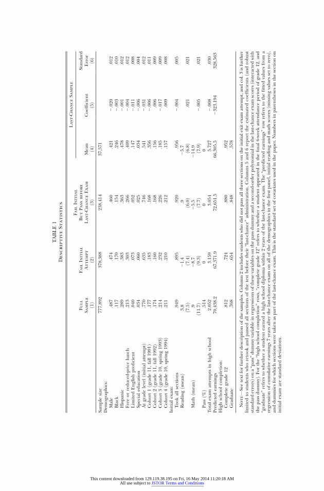
TABLE1

DescriptiveStatistics

Full

Sample

ð1Þ

FailInitial

Attempt

ð2Þ

FailInitial

ButPassbefore

Last-ChanceExam

ð3Þ

Last-ChanceSample

Mean

ð4Þ

Coefficien

tð5Þ

Stan

dard

Error

ð6Þ

Sample

size

777,89

237

8,38

823

8,41

437

,571

Dem

ograp

hics:

Male

.487

.474

.460

.421

2.020

.012

Black

.117

.170

.154

.246

2.003

.010

Hispan

ic.289

.383

.363

.478

2.001

.012

Freeorreduced-price

lunch

.213

.303

.266

.409

2.004

.012

Lim

ited

Englishproficien

t.040

.073

.052

.147

2.011

.008

Specialed

ucation

.034

.060

.025

.034

2.006

.004

Atgrad

elevelðin

itialattemptÞ

.770

.635

.746

.541

2.031

.012

Cohort

1ðgrade11

,fall19

91Þ

.177

.183

.168

.356

2.006

.011

Cohort

2ðgrade11

,fall19

92Þ

.174

.160

.168

.156

.006

.009

Cohort

3ðgrade10

,spring19

93Þ

.214

.232

.226

.185

2.017

.009

Cohort

4ðgrade10

,spring19

94Þ

.211

.210

.212

.157

.009

.008

Initialex

am:

Tookallsections

.949

.895

.920

.956

2.004

.005

Readingðm

eanÞ

3.8

ð7.5Þ

21.4

ð7.4Þ

.9ð6.0Þ

25.7

ð6.8Þ

.021

.021

Mathðm

eanÞ

.9ð11.7Þ

28.7

ð9.3Þ

25.5

ð7.7Þ

214

.9ð7.9Þ

2.005

.021

Passð%

Þ.514

00

0Totalex

amattempts

inhighschool

2.05

23.15

93.05

45.72

72.008

.030

Predictedearnings

70,438

.267

,371

.972

,651

.566

,305

.5232

3.19

432

8.56

3Highschoolco

mpletion:

Complete

grad

e12

.812

.724

.880

.952

Graduate

.768

.654

.848

.578

Note—

Seetext

forfurther

descriptionofthesamples.Column2includes

studen

tswhodid

notpassallthreesectionsontheinitialex

itex

amattempt,an

dco

l.3isfurther

limited

tostuden

tswhoretookan

dpassedallsectionsofthetest

before

their“last-ch

ance”ad

ministration.Columns5an

d6report

theestimated

coefficien

tsðandrobust

stan

darderrorsÞo

na“pass”dummyvariab

lein

regressionsofthesevariab

lesonthepassdummyan

daseco

nd-order

polynomialinthelast-chan

ceex

amscoresðin

teracted

with

thepassdummyÞ.

Forthe“highschoolco

mpletion”rows,“complete

grad

e12

”refers

towhether

astuden

tap

pearedin

thefinal

6-weekattendan

ceperiodofgrad

e12

,an

d“graduate”

refers

towhether

astuden

tearned

ahighschooldiplomawithin

2yearsofthelast-chan

ceex

am.The“predictedearnings”rowrefers

tothefitted

values

from

aregressionofcu

mulative

earnings

7yearsafterthelast-chan

ceex

amonallofthedem

ograp

hicsin

thefirstpan

el,initialread

ingan

dmathscoresðm

issingvalues

setto

zeroÞ,

anddummiesforwhichsectionsweretake

nas

partofthelast-chan

ceex

am.Thisisthestan

dardsetofco

variates

usedin

thepap

er.N

umbersin

paren

theses

inthesectionon

initialex

amarestan

darddeviations.



are much less likely to receive a diploma. Since they have not passed theexit exam before the last-chance administration, this is not surprising.


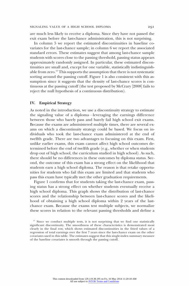
In column 5 we report the estimated discontinuities in baseline co-variates for the last-chance sample; in column 6 we report the associatedstandard errors. These estimates suggest that among last-chance samplestudents with scores close to the passing threshold, passing status appearsapproximately randomly assigned. In particular, these estimated discon-tinuities are small and, except for one variable, statistically indistinguish-able from zero.17 This supports the assumption that there is not systematicsorting around the passing cutoff. Figure 1 is also consistent with this as-sumption since it suggests that the density of last-chance scores is con-tinuous at the passing cutoff ðthe test proposed by McCrary ½2008� fails toreject the null hypothesis of a continuous distributionÞ.

IV. Empirical Strategy

As noted in the introduction, we use a discontinuity strategy to estimatethe signaling value of a diploma—leveraging the earnings differencebetween those who barely pass and barely fail high school exit exams.Because the exams are administered multiple times, there are several ex-ams on which a discontinuity strategy could be based. We focus on in-dividuals who took the last-chance exam administered at the end oftwelfth grade. There are two advantages to focusing on this exam. First,unlike earlier exams, this exam cannot affect high school outcomes de-termined before the end of twelfth grade ðe.g., whether or when studentsdrop out of high school, the curriculum studied in high schoolÞ. As such,there should be no differences in these outcomes by diploma status. Sec-ond, the outcome of this exam has a strong effect on the likelihood thatstudents earn a high school diploma. The reason is that retake opportu-nities for students who fail this exam are limited and that students whopass this exam have typically met the other graduation requirements.Figure 1 confirms that for students taking the last-chance exam, pass-

ing status has a strong effect on whether students eventually receive ahigh school diploma. This graph shows the distribution of last-chancescores and the relationship between last-chance scores and the likeli-hood of obtaining a high school diploma within 2 years of the last-chance exam. Because the exams test multiple subjects, we normalizethese scores in relation to the relevant passing thresholds and define a

17 Since we conduct multiple tests, it is not surprising that we find one statistically
significant discontinuity. The smoothness of these characteristics is demonstrated mostclearly in the final row, which shows estimated discontinuities in the fitted values of aregression of total earnings over the first 7 years since the last-chance exam on the othercovariates used in this table. The estimates suggest that this single-index summary measureof the baseline covariates is smooth through the passing cutoff.


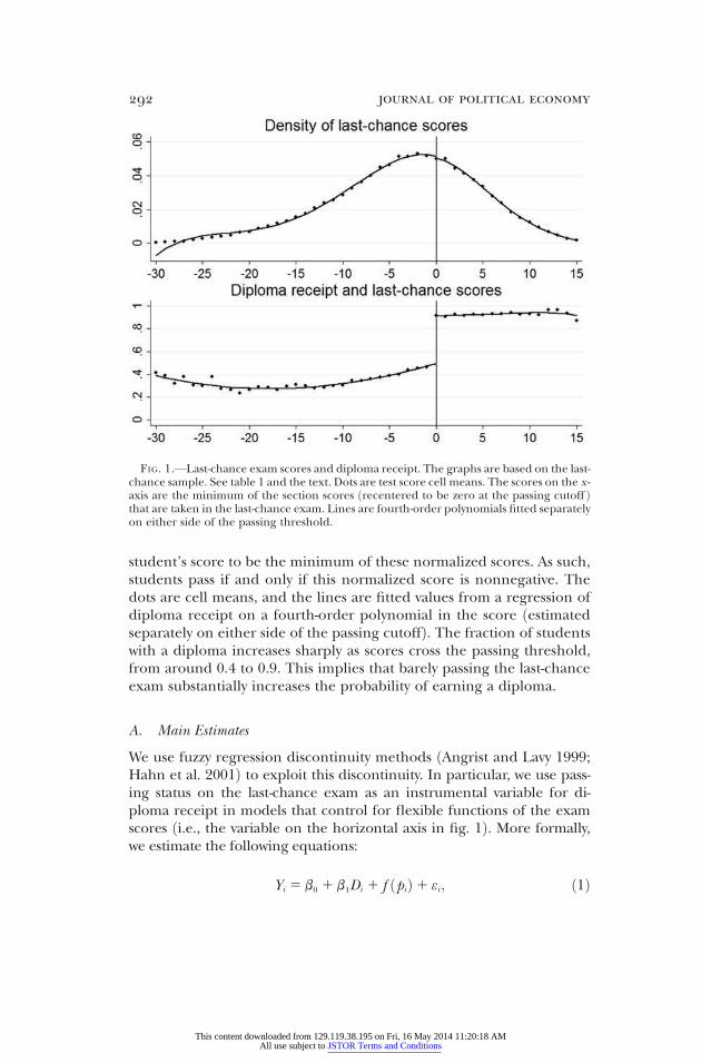
student’s score to be the minimum of these normalized scores. As such,students pass if and only if this normalized score is nonnegative. The

FIG. 1.—Last-chance exam scores and diploma receipt. The graphs are based on the last-chance sample. See table 1 and the text. Dots are test score cell means. The scores on the x -axis are the minimum of the section scores ðrecentered to be zero at the passing cutoff Þthat are taken in the last-chance exam. Lines are fourth-order polynomials fitted separatelyon either side of the passing threshold.


dots are cell means, and the lines are fitted values from a regression ofdiploma receipt on a fourth-order polynomial in the score ðestimatedseparately on either side of the passing cutoffÞ. The fraction of studentswith a diploma increases sharply as scores cross the passing threshold,from around 0.4 to 0.9. This implies that barely passing the last-chanceexam substantially increases the probability of earning a diploma.

A. Main Estimates

We use fuzzy regression discontinuity methods ðAngrist and Lavy 1999;Hahn et al. 2001Þ to exploit this discontinuity. In particular, we use pass-ing status on the last-chance exam as an instrumental variable for di-ploma receipt in models that control for flexible functions of the examscores ði.e., the variable on the horizontal axis in fig. 1Þ. More formally,we estimate the following equations:

Yi 5 b0 1 b1Di 1 f ðpiÞ1 εi ; ð1Þ



Di 5 a0 1 a1PASSi 1 g ðpiÞ1 qi ; ð2Þsignaling value of a high school diploma 293

where Yi represents a given labor market outcome ðe.g., earningsÞ forindividual i, Di denotes high school diploma status, f ðpiÞ captures the
relationship between the outcomes and last-chance scores ðpiÞ, PASSi is anindicator for passing the exam, and εi and qi are error terms. The pa-rameter a1 in the first-stage equation is the discontinuity seen in figure 1.Provided that PASSi and εi are orthogonal, PASSi is a valid instrumentalvariable for Di . This will be true provided that passing status near the cut-off is quasi-randomly assigned and that passing affects earnings only bychanging the likelihood of earning a high school diploma. It also requiresthat differences in the earnings measure we use are informative aboutdifferences in lifetime earnings. We discuss these assumptions below.As with any regression discontinuity application ðLee and Lemieux
2010Þ, we must choose a method for modeling the relationship betweenthe outcomes and the last-chance scores. We use “global polynomial” meth-ods that exploit the full range of scores and specify f and g to be low-order polynomials.18 One set of estimates use polynomials that can takedifferent shapes on either side of the passing cutoff ði.e., fully interactedpolynomials with a passing dummyÞ. Since noninteracted polynomials fitthe reduced-form earnings-score relationship well and since these gen-erate more precise estimates, we also present results based on these morerestrictive specifications.When estimating the earnings discontinuity associated with passing

the exam ðthe parameter a1 in eq. ½2�Þ, we interpret the test score poly-nomial f ðpÞ as a statistical control designed to ensure that those dis-continuity estimates capture the “jump” at the passing threshold. In Sec-tion VI, when we consider the various explanations for our findings, wewill give an economic interpretation to this estimated earnings-score rela-tionship.

18 As suggested by Lee and Lemieux ð2010Þ, the choice of polynomial was guided byminimizing the Akaike information criterion ðAICÞ statistic. The AIC statistic helps choosea functional form that balances the trade-off between generating a good fit and generatingprecise estimates. TheAIC can suggest different functions for the first-stage and the reduced-form relationships, so we present estimates from models that use the more flexible of thesuggested polynomials for both the first stage and reduced form. The other common ap-proach to obtaining regression discontinuity estimates is to use “local linear”methods, whichuse data within only a narrow bandwidth of the passing cutoff and where f and g are linearfunctions ðinteracted with PASSÞ. When the cross-validation method proposed by Imbensand Lemieux ð2008Þ is used, the optimal bandwidth for the reduced form is fairly wide sincethe test score–earnings relationship is approximately linear. However, the optimal band-width for the first stage is much narrower because of the curvature in the test score–diplomarelationship. With bandwidths this narrow, the estimated signaling effects are less precise.We focus, therefore, on the global polynomial results. Local linear methods generate similarresults ðavailable on requestÞ.



B. Validity Checks


As noted, this strategy will deliver valid estimates of b1 under three as-sumptions: first, the usual regression discontinuity assumption that pass-ing status is quasi-randomly assigned close to the passing cutoff; second,that barely passing or failing the exit exam can affect earnings onlythrough an effect on high school diploma receipt ði.e., the exclusion re-striction necessary for PASS to be a valid instrument for DÞ; and third,that differences in the earnings variables we use must be informativeabout differences in actual lifetime earnings. We now discuss our strate-gies for assessing these assumptions.Quasi randomness of passing status on the last-chance exit exam.—As shown

by Lee ð2008Þ, the key issue here is whether students have precise con-trol over test scores. If not, then passing status among students withscores in the neighborhood of the passing threshold can be consideredrandom. It seems plausible to suppose that students cannot control theirscores on these tests. Moreover, the data are consistent with this asser-tion. As noted above, the distribution of scores is smooth around the pass-ing cutoff, and we find little evidence of discontinuities in predeterminedcharacteristics.Exclusion restriction.—The secondassumptionunderlying our approach

is that diploma status can affect earnings only by affecting the likelihoodof earning a high school diploma. The primary concern here is that pass-ing status may affect earnings by changing the likelihood of earning aGED. To address this concern, we use the framework represented by equa-tions ð1Þ and ð2Þ to estimate the effects of passing status on GED receipt.To preview the results, while passing status does have a statistically sig-nificant effect on this outcome, the magnitude of this effect is too smallto undermine our main findings.Validity of the earnings measures.—One issue with the earnings data we

use is that earnings differences appearing shortly after the last-chanceexammight reflect differences in college enrollment. We address this byshowing that passing the exit exam has no effects on college attainmentand only very short-lived effects on college enrollment.19 A second issue isthat the UI data contain information on total earnings, not hourly wages.To the extent that diploma effects on total earnings could be driven bydiploma effects on hourly wages, employment, and hours worked, theycould differ from diploma effects on hourly wages. There are two reasonswhy we feel comfortable using total earnings to measure diploma effects.First, since workers on either side of the passing cutoff should have sim-

19 The exclusion restriction could also be violated if passing the last-chance exit exam
affects college enrollment and attainment and this has a labor market return independentof any effect operating through high school diplomas. This concern is also addressed withthe empirical evidence showing small effects on college attainment.


ilar labor supply preferences, any differences in employment or hoursworked likely reflect demand-driven employer decisions and hence could


be argued to capture the full effect of diploma receipt. For example, iffirms use credential information when making hiring decisions, theremight be diploma effects on employment. Similarly, if the uncompen-sated wage elasticity of labor supply is positive ðBlundell and MaCurdy1999Þ, any diplomawage premiumwill generate diploma effects on hoursworked.20 Second, total earnings measures enable comparisons with ear-lier signaling studies that used total earnings measures ðTyler et al. 2000;Tyler 2004; Lofstrum and Tyler 2007; Jepsen et al. 2010Þ.A third issue is that, if diploma receipt affects the likelihood of having

false zero earnings, our estimates could be biased. We assess this possi-bility in three ways. First, we consider the plausibility and possible mag-nitude of each reason for false zero earnings. Second, we estimate di-ploma effects for several subgroups of workers for whom the false zeroproblem should be small ðe.g., those living in counties with low federalemployment and out-of-state mobility ratesÞ. Third, we assume that allworkers with zero earnings have false zero earnings but that true earn-ings for these workers are below the conditional quantile ðe.g., medianÞ ofearnings among workers with their observed characteristics. We then es-timate regression discontinuity versions of an instrumental variables quan-tile regression ðIVQRÞ model that will, under this assumption, generateconsistent estimates of the quantile treatment effects on total earnings.21

We also estimate these IVQR models for the subsamples that we thinkare unlikely to have false zero earnings.

V. Results

In this section we present our main estimates of the signaling value ofa high school diploma. We begin by reporting estimates of the impactsof passing the last-chance exam on the probability of receiving a highschool diploma. We then report estimates of the impacts of passing the

20 One caveat to this point is that young adults with higher learning ability may invest in
skill acquisition ðe.g., postsecondary schoolingÞ. However, we present evidence below thatearning a high school diploma does not affect college attainment, which suggests thatearning a high school diploma is unlikely to reduce labor supply via effects on post–highschool education.
21 It is worth noting that this approach takes us part of the way toward estimating effectson hourly wages. In particular, if these subsamples exclude workers with false zero earnings,then we will be assigning zero earnings to workers with true zero earnings. Assuming thatthese workers face potential earnings opportunities below the conditional quantile ofearnings given their observed characteristics ðeven more plausible when we restrict thesample to menÞ, the IVQR model will identify diploma effects on earnings opportunities.The only difference between this approach and similar approaches that focus on hourlywages ð Johnson, Kitamura, and Neal 2000; Neal 2004Þ is that the positive earnings analyzedhere also depend on hours worked.



last-chance exam on earnings and estimates of the impacts of receiving ahigh school diploma on earnings. Finally, we present results that support


the validity of our estimates.

A. First-Stage Estimates

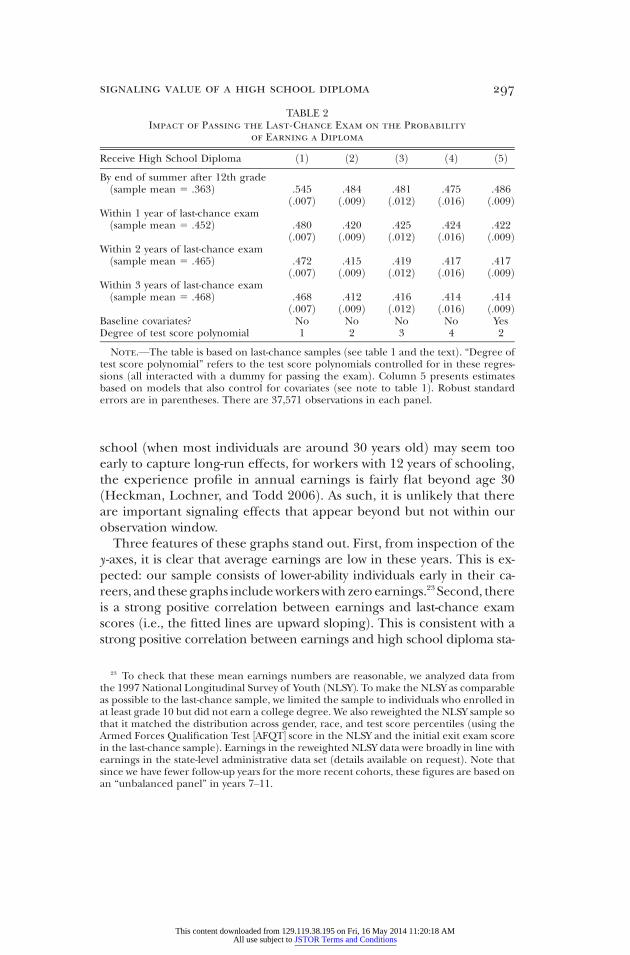
As shown in figure 1, students who pass the last-chance exam are muchmore likely to obtain a high school diploma. To investigate this relationshipin more detail, table 2 reports estimates of the high school diploma effectsof passing the last-chance exam. The first row shows the effect of passingthe exam on the likelihood of receiving a high school diploma by the endof the summer after the last-chance exam. Once wemove beyond a linearspecification, these estimates are robust to the test score polynomial usedðcompare cols. 2–4Þ. The preferred polynomial used in columns 2 and 5ðchosen using goodness-of-fit statisticsÞ suggests estimates of around 0.5.As expected, these are robust to the inclusion of baseline covariatesðcompare cols. 2 and 5Þ.One year after the exam the first-stage discontinuity falls to around

0.42 and remains stable at longer intervals ð2 and 3 yearsÞ. The discon-tinuity falls because some students who fail the last-chance exam passduring the following year or receive a special education waiver. Com-parisons across the different rows of table 2 make clear that we wouldobtain similar results if we considered high school diplomas receivedwithin 1 year or within 3 years of the last-chance exam.

B. Estimates of the Effect of a High School Diploma on Earnings

Figure 2 shows earnings by the last-chance exam score. As before, thedots are cell means, and the lines are fitted values from a regression ofearnings on a fourth-order polynomial in the score ðestimated separatelyon either side of the passing cutoffÞ. The figure shows the present dis-counted value ðPDVÞof earnings ðusing all available years and a discountrate of 0.05, as in Cunha and Heckman ½2007�, as well as earnings inyears 1–3, 4–6, and 7–11 after the last-chance examÞ.22 We examine PDVearnings or earnings pooled across years to streamline the presentationof our results and to generate more precise estimates of the earningseffects of a high school diploma. As discussed below, there is no evidenceto suggest that we lose information by aggregating the data in this way.We chose these particular groupings with a view to capturing earningseffects in the short, medium, and long run. Although 11 years after high

22
We obtain very similar results when using a discount rate of 0.02.


school ðwhen most individuals are around 30 years oldÞ may seem tooearly to capture long-run effects, for workers with 12 years of schooling,

TABLE 2Impact of Passing the Last-Chance Exam on the Probability

of Earning a Diploma

Receive High School Diploma ð1Þ ð2Þ ð3Þ ð4Þ ð5ÞBy end of summer after 12th gradeðsample mean 5 .363Þ .545 .484 .481 .475 .486

ð.007Þ ð.009Þ ð.012Þ ð.016Þ ð.009ÞWithin 1 year of last-chance examðsample mean 5 .452Þ .480 .420 .425 .424 .422

ð.007Þ ð.009Þ ð.012Þ ð.016Þ ð.009ÞWithin 2 years of last-chance examðsample mean 5 .465Þ .472 .415 .419 .417 .417

ð.007Þ ð.009Þ ð.012Þ ð.016Þ ð.009ÞWithin 3 years of last-chance examðsample mean 5 .468Þ .468 .412 .416 .414 .414

ð.007Þ ð.009Þ ð.012Þ ð.016Þ ð.009ÞBaseline covariates? No No No No YesDegree of test score polynomial 1 2 3 4 2

Note.—The table is based on last-chance samples ðsee table 1 and the textÞ. “Degree oftest score polynomial” refers to the test score polynomials controlled for in these regres-sions ðall interacted with a dummy for passing the examÞ. Column 5 presents estimatesbased on models that also control for covariates ðsee note to table 1Þ. Robust standarderrors are in parentheses. There are 37,571 observations in each panel.


the experience profile in annual earnings is fairly flat beyond age 30ðHeckman, Lochner, and Todd 2006Þ. As such, it is unlikely that thereare important signaling effects that appear beyond but not within ourobservation window.Three features of these graphs stand out. First, from inspection of the

y -axes, it is clear that average earnings are low in these years. This is ex-pected: our sample consists of lower-ability individuals early in their ca-reers, and these graphs includeworkerswith zero earnings.23 Second, thereis a strong positive correlation between earnings and last-chance examscores ði.e., the fitted lines are upward slopingÞ. This is consistent with astrong positive correlation between earnings and high school diploma sta-

23 To check that these mean earnings numbers are reasonable, we analyzed data from
the 1997 National Longitudinal Survey of Youth ðNLSYÞ. To make the NLSY as comparableas possible to the last-chance sample, we limited the sample to individuals who enrolled inat least grade 10 but did not earn a college degree. We also reweighted the NLSY sample sothat it matched the distribution across gender, race, and test score percentiles ðusing theArmed Forces Qualification Test ½AFQT� score in the NLSY and the initial exit exam scorein the last-chance sampleÞ. Earnings in the reweighted NLSY data were broadly in line withearnings in the state-level administrative data set ðdetails available on requestÞ. Note thatsince we have fewer follow-up years for the more recent cohorts, these figures are based onan “unbalanced panel” in years 7–11.


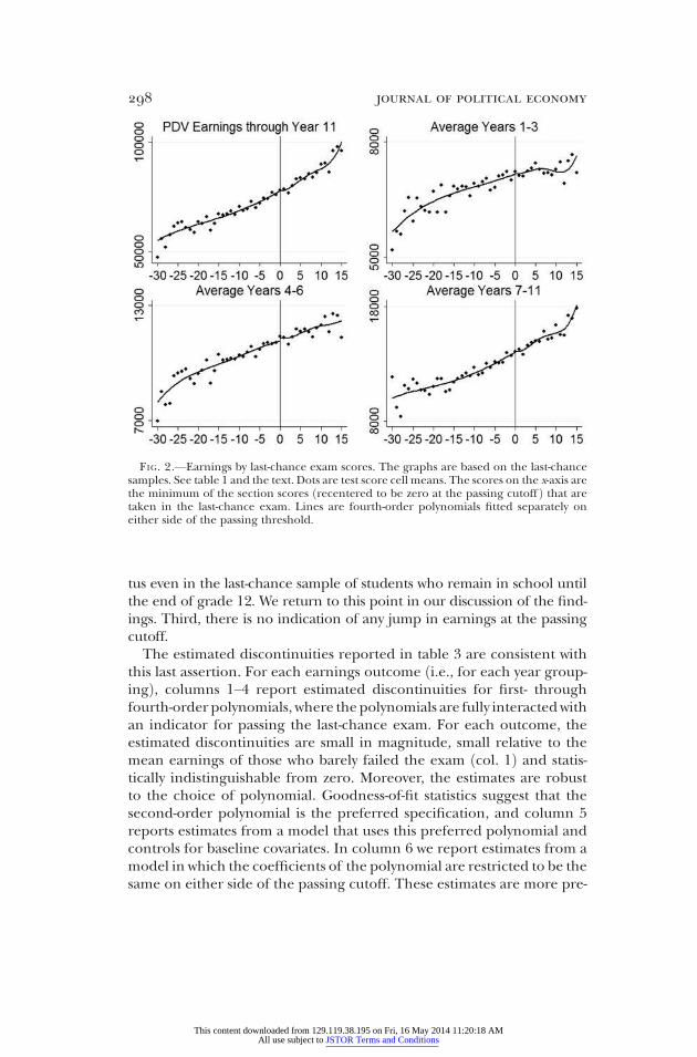
tus even in the last-chance sample of students who remain in school untilthe end of grade 12. We return to this point in our discussion of the find-

FIG. 2.—Earnings by last-chance exam scores. The graphs are based on the last-chancesamples. See table 1 and the text. Dots are test score cell means. The scores on the x-axis arethe minimum of the section scores ðrecentered to be zero at the passing cutoff Þ that aretaken in the last-chance exam. Lines are fourth-order polynomials fitted separately oneither side of the passing threshold.


ings. Third, there is no indication of any jump in earnings at the passingcutoff.The estimated discontinuities reported in table 3 are consistent with

this last assertion. For each earnings outcome ði.e., for each year group-ingÞ, columns 1–4 report estimated discontinuities for first- throughfourth-order polynomials, where thepolynomials are fully interactedwithan indicator for passing the last-chance exam. For each outcome, theestimated discontinuities are small in magnitude, small relative to themean earnings of those who barely failed the exam ðcol. 1Þ and statis-tically indistinguishable from zero. Moreover, the estimates are robustto the choice of polynomial. Goodness-of-fit statistics suggest that thesecond-order polynomial is the preferred specification, and column 5reports estimates from a model that uses this preferred polynomial andcontrols for baseline covariates. In column 6 we report estimates from amodel in which the coefficients of the polynomial are restricted to be thesame on either side of the passing cutoff. These estimates are more pre-



cise than those in column 5, and we cannot reject the hypothesis thatthe coefficients are the same to the left and right of the passing cutoff.


Finally, we obtain similar results when we produce estimates for earningsin single years rather than earnings in particular groups of years.24

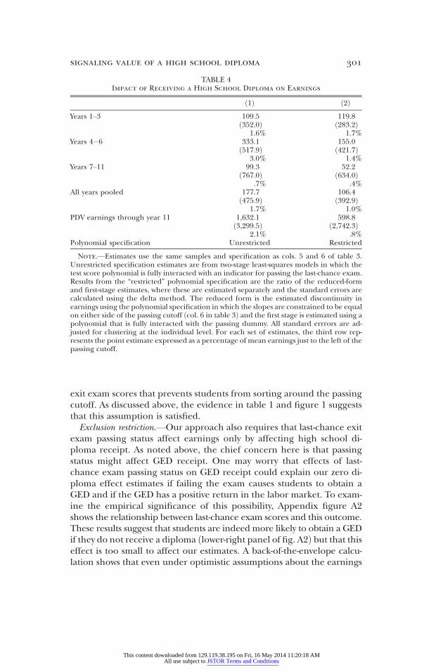
Table 4 reports instrumental variables estimates of the earnings effectsof a high school diploma. Because the reduced-form discontinuities re-ported in table 3 are robust across a variety of specifications, we focus onestimates that use the preferred polynomial and adjust for baseline co-variates. We report estimates based on the restricted polynomial and un-restricted polynomial specifications. The estimated effects are all positivebut never statistically distinguishable from zero and always less than3 percent of the mean earnings of individuals with exit exam scores justbelow the passing cutoff. When we focus on the results for PDVearnings,which combines information across all years, the estimated signalingvalue is only 2 percent of mean PDV earnings in the unrestricted poly-nomial specification and less than 1 percent of mean earnings in the re-stricted polynomial specification.25

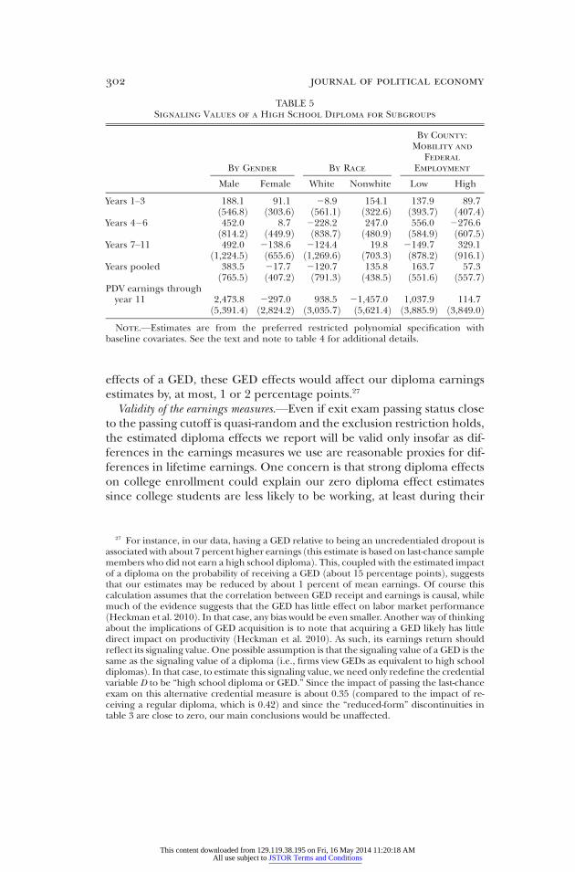
While these estimates suggest that the signaling value of a high schooldiploma is, at most, small, it is possible that signaling values vary acrossdifferent types of workers. To investigate this possibility, the first twopanels of table 5 report separate estimates by race and gender. To savespace, we report estimates only from models that use the restricted ver-sion of the preferred polynomial specification.26 For all subgroups, theestimated returns to a high school diploma are small and not statisti-cally distinguishable from zero. Moreover, for any subgroup comparisonðe.g., men compared to womenÞ, we can never reject the hypothesis thatthe signaling effects are the same.

C. Validity Checks

Quasi randomness of passing status on the last-chance exit exam.—As dis-cussed in Section IV, our approach requires that there be uncertainty in

24 The estimates in years 1–11 are 232 ð135Þ, 45 ð166Þ, 124 ð193Þ, 265 ð214Þ, 118 ð234Þ,
34 ð260Þ, 244 ð281Þ, 238 ð325Þ, 23 ð376Þ, 244 ð476Þ, and 206 ð623Þ. Across all specifica-tions, we can never reject the hypothesis that the earnings effect of passing the last-chanceexam is the same in every year.
25 The 95 percent confidence intervals exclude effects larger than about 10 percent ofmean earnings. In an online appendix, we also report results using data from Florida,which has an exit exam policy similar to that in Texas. The results for Florida are verysimilar, although the data allow us to examine earnings only up to 6 years after takingthe last-chance exam. When we combined the state-specific estimates using the variance-minimizing weights, i.e., the ratio of the inverse variance of the estimate for states to the sumof the inverse variances, to generate more efficient estimates of the earnings effects of ahigh school diploma, we obtain point estimates that are essentially zero and that rule outeffects larger than 5–6 percent of mean earnings ðdetails available on requestÞ.

26 Estimates based on the unrestricted version ðavailable on requestÞ are similar.



TABLE3

ImpactofPassingtheLast-ChanceExam

onEarnings

ð1Þ

ð2Þ

ð3Þ

ð4Þ

ð5Þ

ð6Þ

Years1–

3ðm

eanearnings:7,00

6Þ9.7

39.2

229

.48.3

45.7

50.0

ð110

.8Þ

ð151

.0Þ

ð191

.1Þ

ð233

.5Þ

ð146

.8Þ

ð118

.1Þ

Years4–6ðm

eanearnings:11

,055

Þ18

.272

.170

.216

0.8

138.9

64.6

ð165

.4Þ

ð222

.5Þ

ð281

.1Þ

ð343

.9Þ

ð215

.9Þ

ð175

.9Þ

Years7–

11ðm

eanearnings:13

,732

Þ13

4.6

226

.5213

8.8

87.7

40.3

21.2

ð237

.6Þ

ð319

.7Þ

ð401

.7Þ

ð496

.2Þ

ð311

.0Þ

ð257

.5Þ

Allyearspooledðm

eanearnings:10

,743

Þ58

.025

.8237

.485

.773

.344

.0ð151

.4Þ

ð203

.5Þ

ð255

.4Þ

ð312

.9Þ

ð196

.4Þ

ð162

.3Þ

PDVearnings

through

year

11ðm

ean:75

,986

Þ31

8.6

1.5

251

9.6

169 .2

680.5

249.7

ð1,084

.9Þ

ð1,456

.3Þ

ð1,824

.5Þ

ð2,224

.7Þ

ð1,375

.8Þ

ð1,143

.8Þ

Baselineco

variates?

No

No

No

No

Yes

Yes

Deg

reeoftest

score

polynomial

12

34

22

Polynomialspecification

Unrestricted

Unrestricted

Unrestricted

Unrestricted

Unrestricted

Restricted

Note.—Estim

ates

inthefirstfourrowswerege

nerated

from

apan

eldatasetin

whicheach

observationrepresentsaperson-year,whereyear

den

otes

timesince

thelast-chan

ceex

am,andstan

darderrorsad

justed

forclusteringat

theindividuallevelare

inparen

theses.E

stim

ates

inthefifthrowarefrom

anindividual-le

veldatasetin

whichtheoutcomeisthePDVofearnings

ðr5

.05Þ

through

thelastavailable

year

ðyear

7forthelatestco

hort,year

11forthe

earliest

cohortÞ,an

drobust

stan

darderrors

arein

paren

theses.Meanearnings

refers

tothemeanjust

totheleftofthepassingcu

toffðsc

ore

521Þ.

Estim

ates

inco

ls.1–

4aretheco

efficien

tsonan

indicatorforpassingthelast-chan

ceex

amco

ntrollingforapolynomialin

thelast-chan

ceex

amðfu

lly

interacted

withan

indicatorforpassingÞ

that

isfullyinteracted

withyear

dummies.Estim

ates

inco

l.5includebaselineco

variates

ðsameas

those

usedin

table

2Þfullyinteracted

withyear

dummies.Estim

ates

inco

l.6use

thepreferred

polynomialðquad

raticÞ,

wherethepolynomialisnotinteracted

witha

dummyforpassing.



exit exam scores that prevents students from sorting around the passingcutoff. As discussed above, the evidence in table 1 and figure 1 suggests

TABLE 4Impact of Receiving a High School Diploma on Earnings

ð1Þ ð2ÞYears 1–3 109.5 119.8

ð352.0Þ ð283.2Þ1.6% 1.7%

Years 4–6 333.1 155.0ð517.9Þ ð421.7Þ

3.0% 1.4%Years 7–11 99.3 52.2

ð767.0Þ ð634.0Þ.7% .4%

All years pooled 177.7 106.4ð475.9Þ ð392.9Þ

1.7% 1.0%PDV earnings through year 11 1,632.1 598.8

ð3,299.5Þ ð2,742.3Þ2.1% .8%

Polynomial specification Unrestricted Restricted

Note.—Estimates use the same samples and specification as cols. 5 and 6 of table 3.Unrestricted specification estimates are from two-stage least-squares models in which thetest score polynomial is fully interacted with an indicator for passing the last-chance exam.Results from the “restricted” polynomial specification are the ratio of the reduced-formand first-stage estimates, where these are estimated separately and the standard errors arecalculated using the delta method. The reduced form is the estimated discontinuity inearnings using the polynomial specification in which the slopes are constrained to be equalon either side of the passing cutoff ðcol. 6 in table 3Þ and the first stage is estimated using apolynomial that is fully interacted with the passing dummy. All standard errrors are ad-justed for clustering at the individual level. For each set of estimates, the third row rep-resents the point estimate expressed as a percentage of mean earnings just to the left of thepassing cutoff.


that this assumption is satisfied.Exclusion restriction.—Our approach also requires that last-chance exit

exam passing status affect earnings only by affecting high school di-ploma receipt. As noted above, the chief concern here is that passingstatus might affect GED receipt. One may worry that effects of last-chance exam passing status on GED receipt could explain our zero di-ploma effect estimates if failing the exam causes students to obtain aGED and if the GED has a positive return in the labor market. To exam-ine the empirical significance of this possibility, Appendix figure A2shows the relationship between last-chance exam scores and this outcome.These results suggest that students are indeed more likely to obtain a GEDif they do not receive a diploma ðlower-right panel of fig. A2Þ but that thiseffect is too small to affect our estimates. A back-of-the-envelope calcu-lation shows that even under optimistic assumptions about the earnings



effects of a GED, these GED effects would affect our diploma earningsestimates by, at most, 1 or 2 percentage points.27

TABLE 5Signaling Values of a High School Diploma for Subgroups

By Gender By Race

By County:

Mobility and

Federal

Employment

Male Female White Nonwhite Low High

Years 1–3 188.1 91.1 28.9 154.1 137.9 89.7ð546.8Þ ð303.6Þ ð561.1Þ ð322.6Þ ð393.7Þ ð407.4Þ

Years 4–6 452.0 8.7 2228.2 247.0 556.0 2276.6ð814.2Þ ð449.9Þ ð838.7Þ ð480.9Þ ð584.9Þ ð607.5Þ

Years 7–11 492.0 2138.6 2124.4 19.8 2149.7 329.1ð1,224.5Þ ð655.6Þ ð1,269.6Þ ð703.3Þ ð878.2Þ ð916.1Þ

Years pooled 383.5 217.7 2120.7 135.8 163.7 57.3ð765.5Þ ð407.2Þ ð791.3Þ ð438.5Þ ð551.6Þ ð557.7Þ

PDV earnings throughyear 11 2,473.8 2297.0 938.5 21,457.0 1,037.9 114.7

ð5,391.4Þ ð2,824.2Þ ð3,035.7Þ ð5,621.4Þ ð3,885.9Þ ð3,849.0ÞNote.—Estimates are from the preferred restricted polynomial specification with

baseline covariates. See the text and note to table 4 for additional details.


Validity of the earnings measures.—Even if exit exam passing status closeto the passing cutoff is quasi-random and the exclusion restriction holds,the estimated diploma effects we report will be valid only insofar as dif-ferences in the earnings measures we use are reasonable proxies for dif-ferences in lifetime earnings. One concern is that strong diploma effectson college enrollment could explain our zero diploma effect estimatessince college students are less likely to be working, at least during their

27
For instance, in our data, having a GED relative to being an uncredentialed dropout isassociated with about 7 percent higher earnings ðthis estimate is based on last-chance samplemembers who did not earn a high school diplomaÞ. This, coupled with the estimated impactof a diploma on the probability of receiving a GED ðabout 15 percentage pointsÞ, suggeststhat our estimates may be reduced by about 1 percent of mean earnings. Of course thiscalculation assumes that the correlation between GED receipt and earnings is causal, whilemuch of the evidence suggests that the GED has little effect on labor market performanceðHeckman et al. 2010Þ. In that case, any bias would be even smaller. Another way of thinkingabout the implications of GED acquisition is to note that acquiring a GED likely has littledirect impact on productivity ðHeckman et al. 2010Þ. As such, its earnings return shouldreflect its signaling value. One possible assumption is that the signaling value of a GED is thesame as the signaling value of a diploma ði.e., firms view GEDs as equivalent to high schooldiplomasÞ. In that case, to estimate this signaling value, we need only redefine the credentialvariable D to be “high school diploma or GED.” Since the impact of passing the last-chanceexam on this alternative credential measure is about 0.35 ðcompared to the impact of re-ceiving a regular diploma, which is 0.42Þ and since the “reduced-form” discontinuities intable 3 are close to zero, our main conclusions would be unaffected.


college years. Our results suggest that there are diploma effects on collegeenrollment but that these are short-lived. In particular, figure A2 shows


that there are effects on enrollment in the year after the last-chance examas well as on enrollment at any point in the 8 years following the last-chance exam. However, we see no effects on enrollment in the secondyear after the last-chance exam, and as discussed above, we find no evi-dence of effects on college attainment.28

Perhaps the most serious threat to our results is the possibility thatreceiving a high school diploma increases the likelihood of having falsezero earnings, such that our estimates of the signaling effect of a highschool diploma are downward biased. In analyses not reported, we foundno evidence to suggest that high school diplomas affected the probabil-ity of having observed zero earnings, but this could still be consistent withimpacts on the probability of having false zero earnings. For instance, di-ploma receipt could increase the likelihood of being employed but in-crease the likelihood of moving out of state. If these effects were the samesize, we would find no impact on the probability of having observed zeroeffects, despite an effect on the probability of having false zero earnings.There are three reasons why we do not think that false zero earnings

are driving our results. First, a consideration of each source of false zerossuggests that these are unlikely to be quantitatively important. With re-gard to federal employment, themost relevant concern for workers in theage range we examine is military enlistment. However, individuals in thelast-chance sample are unlikely to meet the military’s aptitude require-ments, at least assuming a rough correspondence between exit exam andAFQT scores.29 Moreover, our estimates are similar for men and women,even though men are much more likely to enlist in the military. Withregard to out-of-state mobility, we note that census data on out-of-statemobility suggest that any mobility effects are likely small. Among those inthe relevant age group, the out-of-state mobility rate was only 3.4 percenthigher for those with a high school diploma than for those without one.30

28
In results not shown, we also find no effect on enrollment in years 3–8 after the last-chance exam.
29 The military accepts very few applicants below the 31st percentile of the nationalAFQT distribution ðAsch et al. 2008Þ. In contrast, the median initial-attempt score in theTexas last-chance sample is at the 12th percentile of the full-sample distribution.

30 Calculations are based on the 5 percent 2000 Census Public Use Microdata Sample.The out-of-state mobility rate pertains to individuals who were living in Texas 5 years priorto the census and is defined as the percentage of individuals in this group who were livingoutside of Texas as of the 2000 census. The sample is restricted to ð1Þ 23–24-year-olds ðwhowere aged 18–19 5 years ago, roughly the age at which the last-chance exam is takenÞ andð2Þ US natives or individuals who were no older than 14 when they immigrated to theUnited States. We obtained similar results when we restricted the sample to workers whocompleted grade 12 but did not enroll in college.



With regard to the “black” economy, if high school diplomas have a pos-itive signaling value, diploma holders would have incentives to avoid self-


employment and the black economy.31

Second, we estimated effects separately by whether students did or didnot attend high schools in counties with low federal employment andout-of-state mobility rates. Since these factors are related to the likeli-hood of having false zero earnings, then to the extent that false zeroswere driving our results, the estimates for these two groups should bedifferent. The evidence in the lower panel of table 5 provides no indi-cation of such a difference.32 Third, estimates based on a regression dis-continuity instrumental variable quantile treatment effects estimator pro-posedbyFrandsen, Frolich, andMelly ð2010Þ shownoevidenceof diplomasignaling effects. Provided that zero observed earnings imply that trueearnings are below the relevant quantile ðconditional on a worker’s ob-served characteristicsÞ, estimates of the quantile treatment effect will beconsistent.33 We think that this condition is especially plausible for thelow-mobility, low–federal employment sample, and especially for men.Both overall and for various subsamples in which we think that observedzero earnings are likely to be indicative of below-quantile earnings, we

31
Self-employment rates are slightly higher among workers with a high school diplomathan among those without one ðGeorgellis and Wall 2000Þ. However, since it is hard to seehow a diploma benefits self-employed workers, this is unlikely to reflect a causal effect ofdiploma status on self-employment. Similarly, it is plausible that diplomas have no causaleffect or possibly a negative effect on employment in jobs in which the pay is “under thetable.”
32 To identify high out-of-state mobility counties in Texas, we used data from the 2000census on county-level population outflows between 1995 and 2000 and intercensal estimatesof the population of Texas counties in 1995. Counties with out-of-state mobility rates belowthe state median ðweighted by populationÞ, which is about 6 percent, were classified as “low-mobility” counties. To identify counties with high federal employment rates, we obtainedcounty-level data on the number of civilian workers employed by the federal governmentfrom the Office of Personnel Management ðhttp://www.opm.gov/feddata/geograph/00geogra.pdfÞ. To calculate the federal employment rate, wedivided thenumberofworkersemployed by the federal government by the total number of workers in a county ðcollectedfrom the Bureau of Labor Statistics’ Local Area Unemployment Statistics seriesÞ. We classi-fied counties as low–federal employment counties if the federal employment rate was below2 percent ðwhich covers about two-thirds of Texas countiesÞ. One limitation of the federalemployment data is that they include only civilian employment. However, most counties withmilitary bases also have a relatively high percentage of civilian employees working for thefederal government. There are only three counties in Texas with military bases that havefederal employment rates below 2 percent, and these represent only 0.8 percent of the last-chance sample and also have relatively high mobility rates ðand so are excluded from theanalysis when we limit the sample to “low-mobility, low–federal employment” countiesÞ.

33 This is also the idea behind the analysis of the black-white wage gap in Johnson et al.ð2000Þ and Neal ð2004Þ. These papers argue that wage offers for women with certainobservable characteristics ðsuch as long spells on public assistanceÞ are likely to be belowthe quantile regression line and that imputing values of zero for these individuals willmitigate the bias resulting from restricting the sample to employed individuals.



found no instances of statistically significant positive signaling effects forquantiles 0.5, 0.6, and 0.75.34


VI. Discussion

A. Implications and Explanations

We now address two questions raised by our findings. First, what are theirimplications for the potential signaling role of school completion? Al-thoughour estimates of the signaling value of a diploma are based on onlya sample of high school completers ðhence do not speak to this questiondirectlyÞ, the question is important because completion is closely relatedto diploma receipt ðin the setting we consider, school completion is anecessary condition for diploma receiptÞ and has been the focus of muchof the previous literature, going back to the earliest models of labor mar-ket signaling ðSpence 1973Þ. Second, what might explain our findings?With respect to completion, the key point is that most districts do not

offer certificates of completion to students who complete high school butdo not pass the exam. In these districts, a diploma therefore allows stu-dents to signal both their completion ðperseverance, etc.Þ and their scoreðcognitive skillÞ cheaply. In districts that offer certificates of completion, adiploma allows students to signal only their cognitive skill. It follows thatif there is a signaling value to completion, then the diploma signalingvalue should be larger in the districts that do not offer certificates of com-pletion than in the districts that do.To test this hypothesis, we generated separate estimates of the diploma

signaling value in the two sets of districts. As seen in Appendix tables A1and A2, the evidence is not consistent with the above hypothesis. In fact,the estimates for noncertificate districts are smaller than those for cer-tificate districts. For instance, in the latest follow-up period ðyears 7–11Þ,the estimates in noncertificate districts range from2738 to 2,009 and arenever statistically significant; the certificate district estimates range from2,849 to 4,355. While some of these are on the margins of statistical sig-nificance, these are best interpreted as noisy zeros. To summarize, the

34 These results are available on request. We also produced estimates for these subgroupsafter restricting the sample to men, since men are less likely to exit the labor force thanwomen. The main limitation of this approach in this context is that the estimates areimprecise, and hence the confidence intervals are very wide. However, the point estimatesare frequently negative and offer little indication that there are positive signaling effectsmasked by statistical imprecision. For instance, the estimated median regression estimatesusing PDV earnings as the outcome were 27,452 ð23,477Þ for the low-mobility and low–federal employment county sample and 211,900 ð11,135Þ for the high-mobility or high–federal employment county sample.



contrast between estimates in certificate and noncertificate districts isdifficult to reconcile with a scenario in which school completion has an


important signaling value but the diploma does not. Moreover, the mag-nitude and sign of the estimates for noncertificate districts are difficult toreconcile with the hypothesis that employers use high school completionor diploma receipt as a signal of unobserved productivity.With respect to explanations, a useful starting point is the observation

that diploma signaling values will be positive if ð1Þ the diploma containsinformation about relevant productivity differences, ð2Þ diploma receiptcan be observed and verified, and ð3Þ firms cannot obtain this produc-tivity information from other sources.35 A violation of the first conditioncould explain our findings but would leave open the possibility thatother educational indicators that are related to productivity do have asignaling value. However, the data are not consistent with this view. Evenif we assume that the diploma can signal only passing the exam ði.e., if wefocus on completersÞ, the evidence reported in panel A of table 6 sug-gests that there is considerable earnings variation among school com-pleters and that this variation is correlated with diploma receipt. More-over, panel B of table 6 shows that even among workers in the last-chancesample, earnings are strongly related to last-chance exam scores ðsee alsofig. 2Þ and hence diploma status. With regard to the second condition,although firms may not be able to verify diploma status ðas discussed inSec. II.CÞ, we might still expect physical possession of a diploma to havereal value in a world in which completing high school and passing the exitexam were valuable signals of skills.This leaves the third condition as the most likely explanation for our

findings, although it is difficult to pinpoint how firms acquire other pro-ductivity information. Clearly, some will be revealed when applying for ajob ðe.g., interviews, tests of an applicant’s suitabilityÞ and more will berevealed from a short tryout period. Note that these three explanationsare likely connected: the smaller the productivity differences betweenworkers with and without diplomas that firms cannot infer from othersources, the weaker will be their incentives to verify diploma status.

B. Relationship to the Previous Literature

Our main findings, that high school completion and diploma receipthave little signaling value in our setting, differ from those of an olderliterature concerned with the returns to completing twelfth grade con-ditional on completing eleventh grade ðHungerford and Solon 1987;

35 The other key assumption is that the labor market is competitive. Given this and the
other assumptions, diploma status will predict productivity, and firms will therefore pay awage premium for the diploma.


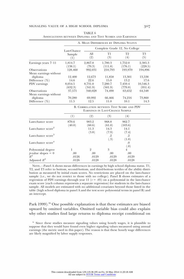
Park 1999Þ.36 One possible explanation is that these estimates are biasedupward by omitted variables. Omitted variable bias could also explain

TABLE 6Associations between Diploma and Test Scores and Earnings

A. Mean Differences by Diploma Status

Last-ChanceSampleð1Þ

Complete Grade 12, No College

Allð2Þ

T1ð3Þ

T2ð4Þ

T3ð5Þ

Earnings years 7–11 1,814.7 2,867.8 1,780.3 1,752.0 2,385.3ð138.1Þ ð79.3Þ ð111.8Þ ð176.1Þ ð228.5Þ

Observations 128,460 992,031 210,793 193,970 194,896Mean earnings withoutdiploma 12,400 12,673 11,858 13,301 13,538

Difference ð%Þ 14.6 22.6 15.0 13.2 17.6PDV earnings 8,054.5 8,731.0 7,280.7 7,459.4 10,546.3

ð632.3Þ ð341.9Þ ð501.9Þ ð779.8Þ ð951.4ÞObservations 37,571 340,028 74,490 63,652 64,548Mean earnings withoutdiploma 70,280 69,992 66,466 74,216 73,860

Difference ð%Þ 11.5 12.5 11.0 10.1 14.3

B. Correlation between Test Score and PDV

Earnings in Last-Chance Sample

ð1Þ ð2Þ ð3Þ ð4ÞLast-chance score 870.6 983.2 968.8 962.7

ð40.0Þ ð60.6Þ ð61.0Þ ð103.6ÞLast-chance score2 11.3 14.3 14.1

ð3.8Þ ð7.9Þ ð7.4ÞLast-chance score3 .2 .2

ð.3Þ ð1.0ÞLast-chance score4 .0

ð.0ÞPolynomial degree 1 2 3 4p -value slopes 5 0 .00 .00 .00 .00R 2 .0126 .0129 .0129 .0129Adjusted R 2 .0126 .0128 .0128 .0128

Note.—Panel A shows mean differences in earnings by high school diploma status. T1,T2, and T3 refer to bottom, second-bottom, and third-bottom tertiles of the ability distri-bution as measured by initial exam scores. No restrictions are placed on the last-chancesample ði.e., we do not restrict to those with no collegeÞ. Panel B shows estimates of aregression of PDV earnings through year 11 ðr 5 .05Þ on a polynomial in the last-chanceexam score ðeach column represents a separate regressionÞ for students in the last-chancesample. All models are estimated with no additional covariates beyond those listed in thetable ðhigh school diploma in panel A and the test score polynomial terms in panel BÞ andan intercept.


why other studies find large returns to diploma receipt conditional on

36 Since these studies measure signaling values using hourly wages, it is plausible tosuppose that they would have found even higher signaling values measured using annual
earnings ðthe metric used in this paperÞ. The reason is that these hourly wage differencesare likely magnified by labor supply responses.


completing twelfth grade ð Jaeger and Page 1996; Frazis 2002Þ. The mainconcern is that firms observe information about workers ðe.g., interview


outcomesÞ not captured in the data sets used in these studies, such thatthe estimates conflate the relevant signaling values with productivity dif-ferences between workers with different levels of education.37 This con-cern is especially relevant since these estimates are typically based on datasets such as the Current Population Survey or census, which have limitedinformation on workers ðHeckman and LaFontaine 2006Þ.Our findings also differ from some of those found in the GED litera-

ture. For example, Tyler et al. ð2000Þ estimate that for some workers, thesignaling value of a GED is between 10 and 20 percent. However, recentwork by Jepsen et al. ð2010Þ estimates GED signaling values closer to zeroand other estimates of the return to a GED, including the Tyler et al.estimates for nonwhites, aremuch smaller ðCameron andHeckman 1993;Heckman and LaFontaine 2006; Lofstrum and Tyler 2007; Jepsen et al.2010Þ.

VII. Conclusion

What is the best framework for thinking about the relationship betweeneducation, productivity, and wages? This is one of the oldest questions ineconomics. The answer has important implications for our understand-ing of various economic phenomena. Since it has implications for the dif-ference between the private and social returns to education, it also hasimportant policy implications.This paper shed light on this question by estimating the signaling value

of a high school diploma, themost commonly held educational credentialin the United States. Since a diploma is a piece of paper, it cannot affectproductivity. Any wage return to a diploma must, therefore, capture itsvalue as a signal of productivity. We use linked administrative data fromTexas to estimate the signaling value of a diploma among students whotake the high school exit exam for the last time. For these students, wefind that a diploma has a signaling value close to zero.Our empirical results do not allow us to draw conclusions about the

signaling value of completing high school and obtaining a diploma for

37 In an important critique of using the wage premium associated with completing 12 vs.11 years of school, Lange and Topel ð2006Þ note that if the productivity returns to edu-
cation are heterogeneous and initially unknown, workers who drop out before completinggrade 12 may be those for whom the returns to education are low. This implies that theobserved returns to completing grade 12 will exceed the observed return to completinggrade 11 even when there is no job market signaling. Riley ð2001Þmakes the more generalpoint that without a theory of why some workers complete twelfth grade while others donot, it is difficult to interpret these estimates. A similar criticism applies to studies thatcompare wages across workers with and without diplomas conditional on highest gradecompleted ð Jaeger and Page 1996; Park 1999Þ: the wage premium may simply reflect thecorrelation between diploma status and characteristics firms but not researchers observe.


other populations. Nevertheless, we have shown that, among this sampleof last-chance exam takers, there is little or no value to the random as-


signment of a low-cost opportunity to signal completing high school andpassing the exit exam. While creative theorists may be able to constructsome variant of the signaling model that accounts for this result, we viewthis evidence as a strong challenge to those who contend that high schoolcompletion is valued by employers as a signal of productivity. Given theevidence in Bishop ð1988Þ concerning the response rates of schools toinquiries about students’ academic records, one expects physical pos-session of a diploma to have real value in a world in which high schoolcompletion is a valuable signal. We find no evidence that Texas studentslive in such a world.

Appendix

A. Exit Exams and High School Graduation Requirements

The Texas class of 1987 was the first that was subject to the state’s exit examrequirement.38 In 1990, changes in state law prompted the adoption of a new,harder set of exams called the Texas Assessment of Academic Skills ðTAASÞ. Thestated purpose of the TAAS was to assess “higher-order thinking skills and prob-lem solving” ðTexas Education Agency 2003Þ.39

The exit-level TAAS consisted of three sections ðreading, math, and writingÞ,all of which had to be passed to satisfy the testing requirement. The math andreading sections had 48 and 60 multiple-choice questions, respectively, and statelaw set the passing standard to be 70 percent. The writing section had a multiple-choice component ð40 questionsÞ and an essay component, which was scored ona four-point scale. The score for the writing section was computed by summingthe multiple-choice items answered correctly and 10 times the essay section, anda passing score was set to be 48.40 The tests are designed to be of equal difficultyacross administrations, but the passing standards are still adjusted to be equiv-alent to the passing standard on the first ðfall 1990Þ exam.41 Students receive ascore report describing their performance on the exam. It contains the scoresreceived on the exam, the standard required to pass each section, and whetherthe student satisfied the graduation requirement.

Students who failed their first attempt could retake the exam during a subse-quent administration ðstudents had to retake only the sections they did not pass

38 This section draws on Texas Education Agency ð2003Þ.39
Students could also take course-specific exams called end-of-course ðEOCÞ exams to
satisfy the testing requirement. The first class for which the EOC exams could be a sub-stitute for the TAAS was 1999 ðthey were not fully phased in until the fall of 1998Þ. Con-sequently, the EOC exams are not relevant for the period in this study.

40 A minimum score of 2 on the writing section was also necessary, which implied that astudent could still fail the writing section with a writing score of 48 or greater if he receiveda 1 on the essay and got 38 out of 40 ðor moreÞ items correct in the multiple-choice section.In practice, very few students scored a 1 on the essay and correctly answered 38 or moremultiple-choice items.

41 These adjustments are typically no more than plus or minus one correct answer.



on an earlier attemptÞ. The timing of the initial exam and retake administrationschanged over the study period. Students in tenth grade in the spring of 1991 or


1992 first took the exam in the fall of eleventh grade. The 1993–95 tenth-gradecohorts began taking the TAAS in the spring of tenth grade. Students in all co-horts could retake the exam during administrations given in the fall, spring, andsummer. Beginning with the 1992 tenth-grade cohort, seniors who had not yetpassed could take the exam one more time before graduation during a specialadministration given in April or May. Thus the number of chances to retake theexam before the end of twelfth grade ðfor students not held backÞ increasedfrom five ðfor students in the 1991 tenth-grade cohortÞ to eight ðfor students inthe 1993–95 tenth-grade cohortsÞ. Texas law requires that districts provide reme-dial services for students who fail the exam ðbut does not mandate specific inter-ventionsÞ.

To receive the “minimum high school program” diploma ðthe easiest highschool diploma to obtainÞ, students had to meet the exit exam requirement andearn a minimum number of course credits across a required distribution of sub-ject areas. Students could receive special education exemptions from the exitexam ðor certain sections of the exit examÞ and still earn high school diplomas.To receive an exemption, a student’s admission, review, and dismissal ðARDÞ com-mittee has to determine that the TAAS is not an appropriate measure of his orher academic progress.42 In Texas during this period, about 7 percent of studentsreceived exemptions from at least one section of the exam ðMartorell 2005Þ. Texasdoes not offer a certificate of completion to students who completed all othergraduation requirements aside from the exit exam. Individual districts, however,can issue these.

Students who complete all other graduation requirements but fail the examand do not receive an exemption can attempt the exam after they leave school. Ifthey pass, they are awarded a diploma. To help prepare to retake the TAAS, stu-dents who have not graduated are also eligible to enroll in school for all or partof an academic year following their twelfth-grade year ða “thirteenth year”Þ.

Texas does not have statewide college admissions standards. However, there areseveral ways in which not having a high school diploma could affect college at-tendance. First, there may be explicit admissions barriers. Four-year colleges typi-cally do not admit students who did not graduate from high school ðunless theyearned a GED degree or a similar “equivalency” credentialÞ. Most community col-leges are “open enrollment” and will admit anyone who wants to enroll, but somecolleges have additional hurdles that students without a high school diploma orGEDmust overcome. For instance, Austin Community College will admit studentswithout a high school diploma or GED only if they “can demonstrate skill profi-ciencies that support an ability to benefit from college-level instruction.” Second,there may be informational barriers. Students might not know that they couldenroll in a community college without a diploma even if they could. Finally, stu-dents without a diploma or GED are ineligible for federal student financial aid.43

42 An ARD committee is made up of teachers, parents, and individuals with expertise
working with special education students.
43 See http://studentaid.ed.gov/eligibility/infographic-accessible for federal studentfinancial aid eligibility information.



B. Data


The Texas data used in this paper come from the Texas Schools Project ðTSPÞ, acollection of administrative records from various Texas state agencies. Thesepermit a longitudinal analysis of individuals as they proceed through high schooland later as they enter college or the workforce.

For this study we used five cohorts of students, defined in terms of the year inwhich they first took the exit exam. These include students who took the initialexam in eleventh grade in the fall of 1991 and 1992 and students who took theinitial exam in tenth grade in the spring of 1993–95. Assuming no grade repeti-tion, these correspond to the 1993–97 graduation classes. The initial exam recordforms the basis for the sample, and for each student in the cohorts we examine,we merged in data from the following Texas Education Agency ðTEAÞ files:

1. Exam files: There are separate files for each exit exam administration. Weused these to generate longitudinal exam-taking histories through 2002.One important limitation is that only scores from the spring 1998 ad-ministration are included in the 1997–98 school year. Thus, we have in-complete data on retakes in the year after the final cohort of students wasin twelfth grade.

2. K–12enrollmentfiles: TheTSPcontains annual enrollmentfiles from1990–2002. These files include fields for school, grade level, special educationstatus, limited English proficiency, and economic disadvantage status.

3. K–12 attendance files: These contain data on 6-week attendance periodsðsix per school yearÞ starting in 1993. These files contain the number ofdays a student attended a given school in each attendance period.

4. GED files: These are annual files that contain GED scores for individualswho attended Texas public schools and who earned a GED certificatethrough 2002. Beginning in 1995, records for all GED test takers are in-cluded regardless of eventual passing status.

5. Graduation files: These are annual rosters of students receiving a highschool diploma from a Texas public school between 1992 and 2001. Thedata distinguish between basic andmore advanced diplomas. Since the exitexam is a requirement for the most basic diploma, we do not make use ofinformation on degree type.

We also merged in data from the following Texas Higher Education Coordi-nating Board ðTEAÞ files ðall files available 1990–2005Þ:

1. Report 1: These files, created every semester, include basic information forstudents enrolled in Texas colleges including the school, semester, andyear in which a student was enrolled.

2. Report 2: These files, created every semester, include information on ad-missions tests, remediation status, placement exam results, and academiccredits attempted in each semester. Academic credits are those that counttoward a degree, and “attempted” credits refer to credits in courses inwhich a student earns a grade ði.e., he did not drop out of the courseÞ butdid not necessarily pass.



3. Report 9: These are annual rosters of awards issued by public colleges inTexas. These files identify the type of degree ðassociate degree or bacca-


laureate degreeÞ.

We also merged in data from Texas Workforce Commission Files ðavailable1990–2004:Q3Þ. These quarterly files contain earnings reported by employerscovered by the state’s UI system. “Year 1” earnings are computed as the sum ofearnings received in quarter 4 of the year of the last-chance exam and quar-ters 1–3 of the following year. Annual earnings for subsequent years are definedin a similar fashion.

Records were linked across files using a unique scrambled student identifica-tion used by the TEA. Records were linked across agencies ðe.g., TEA to TexasWorkforce Commission matchesÞ using scrambled Social Security numbers. Wechecked to see if records matched on the basis of scrambled student identifica-tions or Social Security numbers were in agreement on variables such as genderand date of birth. In general, these fields were almost always in agreement.



C. Additional Figures and Tables

FIG. A1.—Sample Texas high school transcript



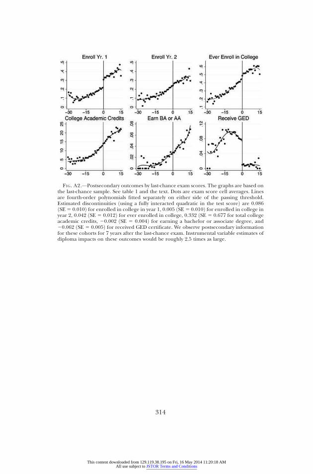
FIG. A2.—Postsecondary outcomes by last-chance exam scores. The graphs are based onthe last-chance sample. See table 1 and the text. Dots are exam score cell averages. Linesare fourth-order polynomials fitted separately on either side of the passing threshold.Estimated discontinuities ðusing a fully interacted quadratic in the test scoreÞ are 0.086ðSE5 0.010Þ for enrolled in college in year 1, 0.005 ðSE5 0.010Þ for enrolled in college inyear 2, 0.042 ðSE 5 0.012Þ for ever enrolled in college, 0.332 ðSE 5 0.677 for total collegeacademic credits, 20.002 ðSE 5 0.004Þ for earning a bachelor or associate degree, and20.062 ðSE 5 0.005Þ for received GED certificate. We observe postsecondary informationfor these cohorts for 7 years after the last-chance exam. Instrumental variable estimates ofdiploma impacts on these outcomes would be roughly 2.5 times as large.

314



TABLEA1

ImpactofReceivingaHighSchoolDiplomaonEarningsinDistricts

ThatDoNotIssueCertificatesofCompletion

NoBaselineCovariates

BaselineCovariates

Unrestricted

ð1Þ

Restricted

ð2Þ

Unrestricted

ð3Þ

Restricted

ð4Þ

Unrestricted

ð5Þ

Restricted

ð6Þ

Unrestricted

ð7Þ

Restricted

ð8Þ

Unrestricted

ð9Þ

Restricted

ð10Þ

Unrestricted

ð11Þ

Restricted

ð12Þ

Years1–

3*253

5.4

248

4.8

223

.9250

8.9

79.1

247

6.1

253

6.2

252

1.1

263

.5251

8.4

272

.9247

2.1

ð704

.8Þ

ð556

.0Þ

ð890

.7Þ

ð517

.6Þ

ð1,158

.0Þ

ð700

.8Þ

ð689

.3Þ

ð545

.3Þ

ð894

.1Þ

ð515

.1Þ

ð1,139

.3Þ

ð686

.1Þ

Years4–6

21,06

3.2

296

7.7

258

3.9

21,00

6.6

250

5.8

21,06

8.3

289

3.0

297

5.9

268

9.6

290

6.3

255

8.6

21,03

2.2

ð1,030

.3Þ

ð832

.5Þ

ð1,285

.2Þ

ð765

.3Þ

ð1,668

.3Þ

ð1,031

.9Þ

ð1,006

.1Þ

ð814

.9Þ

ð1,285

.8Þ

ð760

.1Þ

ð1,632

.3Þ

ð1,007

.1Þ

Years7–

11252

9.8

246

7.6

111.4

267

8.6

1,94

5.5

212

2.5

248

4.8

264

3.5

212

6.8

273

7.6

2,00

9.1

220

2.8

ð1,470

.0Þ

ð1,223

.4Þ

ð1,786

.4Þ

ð1,095

.7Þ

ð2,395

.8Þ

ð1,485

.9Þ

ð1,423

.7Þ

ð1,187

.0Þ

ð1,773

.0Þ

ð1,091

.7Þ

ð2,301

.8Þ

ð1,436

.0Þ

Allyears

pooled

270

4.7

263

3.8

215

7.4

273

0.0

526.9

254

2.9

263

3.9

271

1.0

228

8.4

272

1.3

487.3

255

8.1

ð929

.9Þ

ð760

.2Þ

ð1,146

.8Þ

ð690

.7Þ

ð1,503

.9Þ

ð935

.8Þ

ð900

.7Þ

ð738

.3Þ

ð1,137

.7Þ

ð683

.2Þ

ð1,453

.0Þ

ð905

.6Þ

PDV earnings

through

year

1124,85

4.2

27,04

5.9

24,85

4.2

26,44

3.5

24,85

4.2

24,19

8.7

24,01

5.3

25,48

8.9

24,01

5.3

24,98

0.8

24,01

5.3

24,02

9.6

ð6,549

.3Þ

ð5,391

.5Þ

ð6,549

.3Þ

ð5,473

.4Þ

ð6,549

.3Þ

ð6,589

.8Þ

ð6,222

.1Þ

ð5,121

.1Þ

ð6,222

.1Þ

ð5,199

.8Þ

ð6,222

.1Þ

ð6,250

.8Þ

Degreeof

testscore

polynomial

23

42

34

NOTE.—

Thesample

isbased

onstuden

tswhowerein

districtsthat

did

notoffer

certificatesofco

mpletionan

dwerein

thelargest35

districtsði.e.,thedistrictsforwhichwe

haveinform

ation

on

certificatesofco

mpletionÞ.

Unrestricted

specification

estimates

arefrom

two-stage

least-squares

modelsin

which

thetest

score

polynomialis

fully

interacted

withan


ceex

am.Resultsfrom

therestricted

polynomialspecificationaretheratioofthereduced-form

andfirst-stageestimates,

wheretheseareestimated

separatelyan

dthestan

darderrors

arecalculatedusingthedelta

method.Thereducedform

istheestimated

disco

ntinuityin

earnings

usingthe

polynomialspecificationin

whichtheslopes

areco

nstrained

tobeeq

ual

oneither

sideofthepassingcu

toffan

dthefirststageisestimated

usingapolynomialthat

isfully

interacted

withthepassingdummy.Allstan

darderrorsaread

justed

forclusteringat

theindividuallevel.Se

ethenotesto

tables3an

d4forad

ditionaldetailsonthesampleused

andtheregressionspecifications.

*Meanearnings

areas

follows:foryears1–

3,$6

,923

;foryears4–6,

$11,51

8;foryears7–1

1,$1

4,23

4;forallyearspooled,$1

1,02

3;an

dforPDVearnings

through

year

11,

$77,38

3.

315



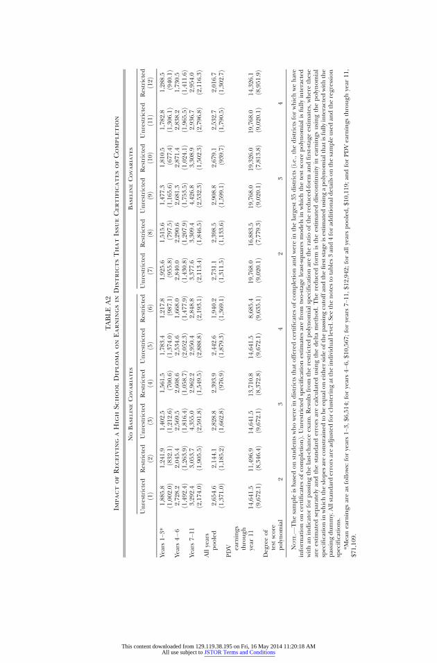
TABLEA2

ImpactofReceivingaHighSchoolDiplomaonEarningsinDistrictsThatIssueCertificatesofCompletion

NoBaselineCovariates

BaselineCovariates

Unrestricted

ð1Þ

Restricted

ð2Þ

Unrestricted

ð3Þ

Restricted

ð4Þ

Unrestricted

ð5Þ

Restricted

ð6Þ

Unrestricted

ð7Þ

Restricted

ð8Þ

Unrestricted

ð9Þ

Restricted

ð10Þ

Unrestricted

ð11Þ

Restricted

ð12Þ

Years1–3

*1,88

5.8

1,24

1.9

1,40

2.5

1,56

1.5

1,78

3.4

1,21

7.8

1,92

5.6

1,51

5.6

1,47

7.3

1,81

0.5

1,78

2.8

1,28

8.5

ð1,002

.0Þ

ð832

.1Þ

ð1,212

.6Þ

ð700

.6Þ

ð1,374

.0Þ

ð987

.1Þ

ð955

.8Þ

ð797

.5Þ

ð1,165

.6Þ

ð677

.4Þ

ð1,306

.1Þ

ð940

.1Þ

Years4–6

2,72

8.2

2,04

5.4

2,56

9.5

2,60

8.6

2,53

4.6

1,66

8.0

2,84

0.0

2,29

0.6

2,68

1.3

2,87

1.4

2,83

8.2

1,73

0.5

ð1,492

.4Þ

ð1,263

.9Þ

ð1,816

.4Þ

ð1,058

.7Þ

ð2,052

.3Þ

ð1,477

.9Þ

ð1,430

.8Þ

ð1,207

.9Þ

ð1,753

.5Þ

ð1,024

.1Þ

ð1,965

.5Þ

ð1,411

.6Þ

Years7–1

13,29

2.4

3,05

3.7

4,35

5.0

2,96

2.2

2,95

0.4

2,84

8.8

3,37

7.6

3,30

9.4

4,42

6.8

3,30

8.9

2,93

6.7

2,95

4.0

ð2,174

.0Þ

ð1,905

.5Þ

ð2,591

.8Þ

ð1,549

.5Þ

ð2,888

.8Þ

ð2,193

.1Þ

ð2,113

.4Þ

ð1,846

.5Þ

ð2,532

.3Þ

ð1,502

.3Þ

ð2,796

.8Þ

ð2,116

.3Þ

Allyears

pooled

2,65

4.6

2,14

4.1

2,82

8.8

2,39

3.9

2,44

2.6

1,94

0.2

2,73

1.1

2,39

8.5

2,90

8.8

2,67

9.1

2,53

2.7

2,01

6.7

ð1,371

.0Þ

ð1,185

.2Þ

ð1,662

.8Þ

ð976

.9Þ

ð1,879

.3Þ

ð1,369

.1Þ

ð1,311

.5Þ

ð1,133

.6Þ

ð1,599

.1Þ

ð939

.7Þ

ð1,790

.5Þ

ð1,302

.7Þ

PDV earnings

through

year

1114

,641

.511

,496

.914

,641

.513

,710

.814

,641

.58,68

5.4

19,768

.016

,883

.519

,768

.019

,326

.019

,768

.014

,326

.1ð9,672

.1Þ

ð8,346

.4Þ

ð9,672

.1Þ

ð8,372

.8Þ

ð9,672

.1Þ

ð9,635

.1Þ

ð9,020

.1Þ

ð7,779

.3Þ

ð9,020

.1Þ

ð7,813

.8Þ

ð9,020

.1Þ

ð8,951

.9Þ

Degreeof

testscore

polynomial

23

42

34

NOTE.—

Thesample

isbased

onstuden

tswhowerein

districtsthat

offered

certificatesofco

mpletionan

dwerein

thelargest35

districtsði.e.,thedistrictsforwhichwehave

inform

ationoncertificatesofco

mpletionÞ.Unrestricted

specificationestimates

arefrom

two-stage

least-squares

modelsin

whichthetestscore

polynomialisfullyinteracted

withan


ceex

am.R

esultsfrom

therestricted

polynomialspecificationaretheratioofthereduced-form

andfirst-stageestimates,w

herethese

areestimated

separatelyan

dthestan

darderrors

arecalculatedusingthedelta

method.Thereducedform

istheestimated

disco

ntinuityin

earnings

usingthepolynomial

specificationin

whichtheslopes

areco

nstrained

tobeeq

ualoneither

sideofthepassingcu

toffan

dthefirststageisestimated

usingapolynomialthat

isfullyinteracted

withthe

passingdummy.Allstan

darderrorsaread

justed

forclusteringat

theindividuallevel.Se

ethenotesto

tables3an

d4forad

ditionaldetailsonthesampleusedan

dtheregression

specifications.

*Meanearnings

areas

follows:foryears1–3

,$6

,514

;foryears4–6,

$10,56

7;foryears7–1

1,$1

2,94

2;forallyearspooled,$1

0,11

9;an

dforPDVearnings

through

year

11,

$71,10

9.



References


Angrist, J., and V. Lavy. 1999. “Using Maimonides’ Rule to Estimate the Effect ofClass Size on Scholastic Achievement.” Q.J.E. 114 ð2Þ: 533–75.

Asch, B., C. Buck, J. Klerman, M. Kleykamp, and D. Loughran. 2008. MilitaryEnlistment of Hispanic Youth: Obstacles and Opportunities. Santa Monica, CA:RAND.

Becker, G. S. 1964. Human Capital: A Theoretical and Empirical Analysis, with SpecialReference to Education. New York: Columbia Univ. Press ðfor NBERÞ.

———. 1967. “Human Capital and the Personal Distribution of Income: AnAnalytical Approach.” Woytinsky Lecture no. 1. Ann Arbor: Inst. Public Admin.,Univ. Michigan.

Bishop, J. 1988. “Employer Testing and Incentives to Learn.” Working Paperno. 433, Center Advanced Human Resource Studies, Indus. and Labor Rela-tions School, Cornell Univ.

Blundell, R., and T. MaCurdy. 1999. “Labor Supply: A Review of AlternativeApproaches.” In Handbook of Labor Economics, vol. 3A, edited by O. Ashenfelterand D. Card. Amsterdam: Elsevier.

Cameron, S., and J. J. Heckman. 1993. “The Nonequivalence of High SchoolEquivalents.” J. Labor Econ. 11 ð1Þ: 1–47.

Cunha, F., and J. J. Heckman. 2007. “The Evolution of Inequality, Heterogeneityand Uncertainty in Labor Earnings in the U.S. Economy.” Working Paperno. 13526, NBER, Cambridge, MA.

Dee, T. S., and B. Jacob. 2007. “Do High School Exit Exams Influence Educa-tional Attainment or Labor Market Performance?” In Standards-Based Reformand Children in Poverty: Evidence from No Child Left Behind, edited by A. Gamoran.Washington, DC: Brookings Inst.

Frandsen, B. R., M. Frolich, and B. Melly. 2010. “Quantile Treatment Effects inthe Regression Discontinuity Design.” Manuscript, Massachusetts Inst. Tech.

Frazis, H. 2002. “Human Capital, Signaling, and the Pattern of Returns to Ed-ucation.” Oxford Econ. Papers 54:298–320.

Georgellis, Y., and H. Wall. 2000. “Who Are the Self-Employed?” Fed. Reserve BankSt. Louis Rev. 82 ð6Þ: 15–23.

Hahn, J., P. Todd, and W. van der Klaauw. 2001. “Identification and Estimation ofTreatments with a Regression Discontinuity Design.” Econometrica 69 ð1Þ: 201–9.

Heckman, J. J., J. Humphries, and N. Mader. 2010. “The GED.” Working Paperno. 16064, NBER, Cambridge, MA.

Heckman, J. J., and P. A. LaFontaine. 2006. “Bias-Corrected Estimates of GEDReturns.” J. Labor Econ. 24 ð3Þ: 661–700.

Heckman, J. J., L. Lochner, and P. Todd. 2006. “Earnings Functions, Rates ofReturn and Treatment Effects: The Mincer Equation and Beyond.” In Hand-book of the Economics of Education, vol. 1, edited by E. Hanushek and F. Welch.Amsterdam: Elsevier.

Hungerford, T., and G. Solon. 1987. “Sheepskin Effects in the Returns to Edu-cation.” Rev. Econ. and Statis. 69:175–77.

Imbens, G. W., and T. Lemieux. 2008. “Regression Discontinuity Designs: AGuide to Practice.” J. Econometrics 142 ð2Þ: 615–35.

Jaeger, D., and M. Page. 1996. “Degrees Matter: New Evidence on SheepskinEffects in the Returns to Education.” Rev. Econ. and Statis. 77:733–39.

Jepsen, C., P. Mueser, and K. Troske. 2010. “Labor Market Returns to the GEDUsing Regression Analysis.” Manuscript, Univ. Kentucky.

Johnson, W., Y. Kitamura, and D. Neal. 2000. “Evaluating a Simple Method forEstimating Black-White Gaps in Median Wages.” A.E.R. 90 ð2Þ: 339–43.



Lange, F., and R. Topel. 2006. “The Social Value of Education and HumanCapital.” InHandbook of the Economics of Education, vol. 1, edited by E. Hanushek


and F. Welch. Amsterdam: Elsevier.Lee, D. S. 2008. “Randomized Experiments from Non-random Selection in U.S.House Elections.” J. Econometrics 142 ð2Þ: 675–97.

Lee, D. S., and T. Lemieux. 2010. “Regression Discontinuity Designs in Eco-nomics.” J. Econ. Literature 48 ð2Þ: 281–355.

Lofstrum, M., and J. Tyler. 2007. “Modeling the Signaling Value of the GED withan Application to an Exogenous Passing Standard Increase in Texas.” IZA Dis-cussion Paper no. 2953, Inst. Study Labor, Bonn.

Lucas, R. E., Jr. 1988. “On the Mechanics of Economic Development.” J. MonetaryEcon. 22:3–42.

Martorell, P. 2005. “Do High School Graduation Exams Matter? Evaluating theEffects of Exit Exam Performance on Student Outcomes.” Manuscript, Univ.California, Berkeley.

McCrary, J. 2008. “Manipulation of the Running Variable in the Regression Dis-continuity Design: A Density Test.” J. Econometrics 142 ð2Þ: 698–714.

Mincer, J. 1974. Schooling, Experience, and Earnings. New York: Columbia Univ.Press.

Moretti, E. 2006. “Private and Social Returns to Education.” Rivista di PoliticaEconomica 96:5–6.

———. 2010. “Local Labor Markets.” In Handbook of Labor Economics, vol. 4B,edited by O. Ashenfelter and D. Card. Amsterdam: Elsevier.

Neal, D. 2004. “The Measured Black-White Wage Gap among Women Is TooSmall.” J.P.E. 112:S1–S28.

Park, J. H. 1999. “Estimation of Sheepskin Effects Using the Old and the NewMeasures of Educational Attainment in the Current Population Survey.” Econ.Letters 62 ð2Þ: 237–40.

Peterson, K. 2005. “High School Exit Exams on the Rise.” Stateline. http://www.pewstates.org/projects/stateline/headlines/high-school-exit-exams-on-the-rise-85899389823.

Riley, J. G. 2001. “Silver Signals: Twenty-Five Years of Screening and Signaling.”J. Econ. Literature 39 ð2Þ: 432–78.

Romer, P. 1990. “Endogenous Technological Change.” J.P.E. 98:S71–S102.Spence, M. 1973. “Job Market Signaling.” Q.J.E. 83:355–79.Texas Education Agency. 2003. Timeline of Testing in TEXAS. http://web.archive.org/web/20090107000128/http://ritter.tea.state.tx.us/student.assessment/resources/studies/testingtimeline.pdf.

Tyler, J. H. 2004. “What Is the Value of the GED to Dropouts Who Pursue theCredential?” Indus. and Labor Relations Rev. 57 ð4Þ: 587–98.

Tyler, J. H., R. Murnane, and J. Willett. 2000. “Estimating the Labor MarketSignaling Value of the GED.” Q.J.E. 115:431–68.

Zabala, D., A. Minnici, J. McMurrer, D. Hill, A. Bartley, and J. Jennings. 2007.“State High School Exit Exams 2007 Annual Report: Working to Raise TestScores.” Center on Education Policy, Washington, DC.



The Signaling Value of a High School Diplomafaculty.smu.edu/millimet/classes/eco7321/papers/clark...

Documents

Transcript of The Signaling Value of a High School Diplomafaculty.smu.edu/millimet/classes/eco7321/papers/clark...