University of Pennsylvania University of Pennsylvania

ScholarlyCommons ScholarlyCommons

Health Care Management Papers Wharton Faculty Research

8-2011

The Short-Term and Localized Effect of Gun Shows: Evidence The Short-Term and Localized Effect of Gun Shows: Evidence

from California and Texas from California and Texas

Mark Duggan University of Pennsylvania

Randi Hjalmarsson

Brian. A. Jacob

Follow this and additional works at: https://repository.upenn.edu/hcmg_papers

Part of the Business Law, Public Responsibility, and Ethics Commons, Other Business Commons, and

the Other Mental and Social Health Commons

Recommended Citation Recommended Citation Duggan, M., Hjalmarsson, R., & Jacob, B. A. (2011). The Short-Term and Localized Effect of Gun Shows: Evidence from California and Texas. Review of Economics and Statistics, 93 (3), 786-799. http://dx.doi.org/10.1162/REST_a_00120

This paper is posted at ScholarlyCommons. https://repository.upenn.edu/hcmg_papers/134 For more information, please contact repository@pobox.upenn.edu.

The Short-Term and Localized Effect of Gun Shows: Evidence from California and The Short-Term and Localized Effect of Gun Shows: Evidence from California and Texas Texas

Abstract Abstract We examine the effect of more than 3,400 gun shows using data from Gun and Knife Show Calendar and vital statistics data from California and Texas. Considering the one month following each show and a surrounding area ranging from 80 to 2,000 square miles, we find no evidence that gun shows increase either gun homicides or suicides. The similarity of our estimates for California and Texas suggests that the much tighter California gun show regulations do not substantially reduce the number of firearms-related deaths in that state. Using incident-level crime data for Houston, Texas, we also find no evidence of an effect on other crime categories.

Disciplines Disciplines Business Law, Public Responsibility, and Ethics | Other Business | Other Mental and Social Health

This journal article is available at ScholarlyCommons: https://repository.upenn.edu/hcmg_papers/134

THE SHORT-TERM AND LOCALIZED EFFECT OF GUN SHOWS: EVIDENCE

FROM CALIFORNIA AND TEXAS

Mark Duggan, Randi Hjalmarsson, and Brian A. Jacob

Abstract—We examine the effect of more than 3,400 gun shows usingdata from Gun and Knife Show Calendar and vital statistics data fromCalifornia and Texas. Considering the one month following each showand a surrounding area ranging from 80 to 2,000 square miles, we find noevidence that gun shows increase either gun homicides or suicides. Thesimilarity of our estimates for California and Texas suggests that themuch tighter California gun show regulations do not substantially reducethe number of firearms-related deaths in that state. Using incident-levelcrime data for Houston, Texas, we also find no evidence of an effect onother crime categories.

I. Introduction

THOUSANDS of gun shows take place in the UnitedStates each year. Gun control advocates argue that the

‘‘gun show loophole’’ makes it easier for potential criminalsto obtain a gun; the loophole basically allows unlicensedvendors at gun shows to sell firearms without conductingbackground checks on purchasers. In support of this claim,gun control advocates commonly cite selected extremeevents, such as the April 20, 1999, Columbine High Schoolshooting during which Eric Harris and Dylan Klebold shot26 students, killing 13. Subsequent investigations by theU.S. Bureau of Alcohol, Tobacco, Firearms, and Explosives(ATF) revealed that a friend of Harris and Klebold had pur-chased some of the weapons used in the shooting at a gunshow (Obmascik, Robinson, & Olinger, 1999). Though notan issue generally raised by gun control advocates, onemight also be concerned that gun shows increase suiciderates by providing individuals considering suicide with amore lethal means of ending their lives. Proponents, how-ever, argue that gun shows are innocuous since potentialcriminals can acquire guns quite easily through other blackmarket sales or theft. Gun lobbyists often cite a U.S. Bureauof Justice Statistics survey that found that only 0.7% ofstate prison inmates who had ever owned a gun reportedthat they obtained it at a gun show (Harlow, 2001).In response to the concerns about gun shows, eighteen

states have closed the gun show loophole by passing legis-lation that regulates the private transfer of firearms, and six

states have imposed additional regulations on gun shows.1

Despite this legislative activity, there is little empirical evi-dence regarding the effect of gun shows and, to our knowl-edge, no studies of the effect of gun shows on gun suicides.2

This stems in large part from the difficulty of obtainingdetailed information on gun shows and outcomes such ascrime or mortality. Moreover, because the timing and loca-tion of gun shows is clearly not random, it is difficult toinfer the causal impact of gun shows by simply comparinggeographical areas with frequent gun shows to those withfewer shows.3

This paper consists of two analyses that study the impactof gun shows on both mortality and crime. The first analysisexamines the impact of gun shows on gun and nongun sui-cides and homicides using a unique ZIP code by week-leveldata set of all gun shows and deaths in Texas and Californiafrom 1994 to 2004. During this period, there were morethan 2,200 gun shows in Texas and almost 1,200 gun showsin California.

We chose Texas and California for this analysis for anumber of reasons. As the nation’s two most populousstates, they comprise approximately 20% of the total U.S.population and accounted for 18% of total U.S. gun deathsin 2000 (Office of Statistics and Programming, CDC). Inaddition, these two states account for more than 13% of the8.3 million background checks for firearms transfers con-ducted by the FBI and state agencies in 2005 (Bowlinget al., 2006). They also rank among the top five states interms of the number of gun shows (U.S. Department of Jus-tice and U.S. Department of Treasury, 1999). Finally, thestates’ gun show regulatory environments differ signifi-cantly: California is known for having the most aggressivegun show regulations, while Texas has none.

Received for publication September 11, 2008. Revision accepted forpublication March 26, 2010.* Duggan: University of Maryland and NBER; Hjalmarsson: Queen

Mary, University of London; Jacob: University of Michigan and NBER.We thank Andrew Cantor, Brittani Head, Joshua Hyman, Rebecca

Kahane, JD LaRock, Emily Owens, Petko Peev, and Paul Vernier fortheir excellent research assistance. We also thank Michael Anderson,Phil Cook, Michael Greenstone, David Hemenway, Ilyana Kuziemko,Jens Ludwig, Garen Wintemute, two anonymous referees, and partici-pants of the MPRC’s Crime and Population Workshop, the NBER’sCrime Working Group Conference, and the 2009 AEA session on Eco-nomic Perspectives on Crime for helpful suggestions. All remainingerrors are our own.

1 States became particularly attentive to the gun show loophole after the1999 Columbine incident and again after the 2007 Virginia Tech mas-sacre. Even though the weapons used in the Virginia Tech shooting werepurchased at federally licensed stores and not gun shows, the VirginiaTech Review Panel (2007) put together a report that recommended requir-ing background checks for firearms sales at gun shows. Governor Kainemade it a priority to enact such a law in 2008, but it was defeated in theVirginia Senate.2 Lott (2003) examines violent crime rates before and after the introduc-

tion of state laws to require background checks for private transfers ofhandguns. Comparing 9 states that closed this loophole by 1994 to 33states that never implemented such laws, he finds no evidence that thesegun show laws reduced violent crime and, in fact, finds that such laws arepositively associated with murder, robbery, and auto theft.3 Lott (2003) finds that laws requiring background checks at gun shows

as well as laws banning assault weapons or imposing waiting periods arenegatively associated with the prevalence of gun shows in a state. He alsofinds that western and rural states tend to have the greatest number of gunshows per capita and that states with higher gun ownership rates have sig-nificantly more shows.

The Review of Economics and Statistics, August 2011, 93(3): 786–799! 2011 by the President and Fellows of Harvard College and the Massachusetts Institute of Technology

To address the potentially endogenous timing and loca-tion of gun shows, we examine outcome trends within juris-dictions where gun shows occur, exploiting the high-fre-quency variation in deaths that we observe in the vitalstatistics data. Our baseline empirical specification esti-mates the impact of a gun show on the number of deaths ina ZIP code in the week of a show and the three subsequentweeks relative to the four weeks preceding a show, control-ling for ZIP code by year fixed effects as well as monthfixed effects. Because ZIP code areas are quite small andbecause the ZIP codes in which gun shows occur may beprimarily commercial (such as a convention center) andattract many attendees from outside the immediate ZIPcode, we also estimate specifications that use the number ofgun shows that take place within various distances to thehome ZIP code.Overall, we find little evidence that gun shows have a

significant effect on each of our four mortality measures:gun homicides, nongun homicides, gun suicides, and non-gun suicides. This finding persists across a variety of speci-fications. First, we arrive at the same finding when estimat-ing our baseline specification separately for California andTexas ZIP codes, despite the differing regulatory environ-ments in each state. Second, the results do not depend onthe geographical area considered: 0, 5, 10, and 25 milesfrom the ZIP code in which the show occurs. Third, thefindings are not sensitive to the estimation strategy used oralternative sets of fixed effects. Finally, we do not find evi-dence of heterogeneous effects over time or across ZIPcodes with differing degrees of poverty, urbanicity, and gunownership.Using a similar empirical methodology, the second ana-

lysis considers the impact of guns shows on gun and non-gun violent crimes, as well as property crimes using a cen-sus tract by week data set of all FBI Part I crime incidentsrecorded by the Houston Police Department from 1994 to2004. We identify the number of shows in each census tractand within various radii of each tract. As in our mortalityanalysis, we find no evidence that gun shows have a signifi-cant effect on crime.Our analysis has two important limitations. First, we

examine only the geographical areas in and around wheregun shows take place. To the extent that guns obtained atshows are transported elsewhere, we do not pick up theseeffects. In addition, our identification strategy relies onhigh-frequency variation that, by definition, focuses onshort-term effects. Specifically, most of our specificationslook for spikes in various measures of mortality and crimein the four weeks immediately following a gun show. How-ever, guns are durable and can be used many years in thefuture, and thus our estimates do not capture these long-runeffects. Despite these limitations, we believe that this analy-sis makes an important contribution to understanding theinfluence of gun shows, the regulation of which has argu-ably been the most active area of federal, state, and localfirearms policy during the past decade.

The remainder of the paper proceeds as follows. SectionII provides background information on gun ownership andthe institutional and legal arrangements surrounding gunshows. Section III describes the data used in the analysis,and section IV outlines our empirical strategy. Section Vpresents our main results, and section VI concludes.

II. Background

A. Gun Ownership in the United States

Firearms manufacturing and ownership in the UnitedStates are substantial. Approximately 5 million new fire-arms were for sale in the United States in 2006, includingnet imports.4 Using the 1994 National Survey of PrivateOwnership of Firearms (NSPOF), Cook and Ludwig (1996)estimate that approximately 192 million privately ownedfirearms, including 65 million handguns, exist in the UnitedStates and that about 35% of households own a gun. In con-trast, the U.S. Bureau of Alcohol, Tobacco and Firearms(U.S. Department of the Treasury, 2000) estimated thatapproximately 242 million firearms were available for saleor owned by civilians in the United States at the end of1996, including roughly 72 million handguns, 76 millionrifles, and 64 million shotguns.

Previous research generally suggests a positive relation-ship between gun ownership rates and both gun suicide andhomicide rates. That is, increases in gun ownership ratesare associated with increases in gun homicide (Duggan,2001; Cook & Ludwig, 2004) and gun suicide (Kellermannet al., 1992; Sloan et al., 1990; Azrael, Hemenway, &Miller, 2002).5

B. Institutional Background on Gun Shows

Thousands of gun shows are held in the United Stateseach year.6 Shows are generally open to the public, thoughattendees often pay a modest admission fee. Most showsare held over the weekend and last for two days, drawing an

4 Specifically, in 2006, approximately 1.4 million handguns and 2.2million shotguns and rifles were manufactured in the United States, withjust 0.3 million of these exported (U.S. Department of the Treasury,2008). According to Census Bureau statistics published by ShootingIndustry magazine, an additional 1.1 million handguns and 0.7 millionrifles and shotguns were imported into the United States. See http://www.shootingindustry.com/Pages/SpecRep6.html#importhand, accessedAugust 29, 2008.5 In contrast, Lott and Mustard (1997) find that crime declined in states

that passed concealed weapons laws, suggesting that gun ownershipreduces crime through deterrence. Though Moody (2001) supports theseresults, Ayres and Donohue (1999) and Black and Nagin (1998) foundthat the results were not robust to a variety of assumptions and modelingchoices.6 Lott (2003) states that roughly 1,900 gun shows were held in the Uni-

ted States in 1991 and that this number increased to a high of 2,907 in1996, but then declined to roughly 2,400 in 2001. Using the same datasource (a periodical titled Gun Show Calendar), the U.S. Department ofJustice and U.S. Department of the Treasury (1999) came up with a muchhigher figure for the overall number of gun shows in 1998: 4,442 showscompared with the 2,600 reported by Lott (2003).

787SHORT-TERM AND LOCALIZED EFFECT OF GUN SHOWS

average of 2,500 to 5,000 people per show. To rent a tablefrom a promoter, vendors pay fees typically ranging from$5 to $50. The number of tables at gun shows rangeswidely, from as few as 50 to as many as 2,000 (U.S. Depart-ment of Justice and U.S. Department of the Treasury,1999).7

The share of guns acquired by private citizens throughgun shows appears relatively small compared to other chan-nels. The NSPOF estimated that approximately 239,000firearms per year were bought at U.S. gun shows and fleamarkets in 1993 and 1994. This represents just 4% of bothlong guns and handguns that private individuals acquiredfrom all sources in those years (Cook & Ludwig, 1996).Similarly, a 1997 survey of 18,000 state prison inmates bythe U.S. Bureau of Justice Statistics found that only 0.7%and 1.7% of inmates who had ever owned a gun said theyhad obtained it at a gun show or flea market, respectively(Harlow, 2001). Yet an ATF study (U.S. Department of theTreasury, 2000) found that 14% of their criminal traffickinginvestigations between 1996 and 1998 involved guns pur-chased from gun shows; about 46% involved straw pur-chases (an individual purchases a gun for someone else),and 20% involved unlicensed sellers.8

C. The Gun Show Loophole

Certain individuals, primarily felons and those convictedof domestic abuse, are prohibited from purchasing or pos-sessing a firearm under federal law.9 The so-called gunshow loophole refers to the fact that federal law requiresfederal firearms licensees (FFLs)—those licensed by thegovernment to manufacture, import, or deal in firearms—toconduct background checks on nonlicensed persons seekingto obtain firearms, but it does not require such checks bythose who transfer firearms and do not meet the statutorytest of being engaged in the business to do so (Krouse,2005). Therefore, whereas a gun dealer operating a gunshop is obliged to conduct background checks on potentialbuyers, private sellers at gun shows who ‘‘transfer’’ firearmsdo not have to do so. These licensees comprise 50% to 75%

of the vendors at most gun shows, so some private venderscould use this loophole to entice potential customers to theirtables (U.S. Department of Justice and U.S. Department ofthe Treasury, 1999).

A number of states, however, have passed legislation reg-ulating at least some of these sales. For example, California,Rhode Island, and the District of Columbia require back-ground checks on all gun purchases, including those at gunshows. Colorado, Connecticut, Illinois, New York, and Ore-gon have less comprehensive regulations but also requirebackground checks for firearms purchased at gun shows(Legal Community against Violence, 2008). The vastmajority of states, however, do not require a backgroundcheck for transactions occurring at gun shows.

Wintemute (2007) compared gun shows in California,which is considered to have ‘‘a uniquely restrictive regula-tory environment for gun shows,’’ with shows in Arizona,Nevada, Texas, and Florida—four states that do not regulateany private party firearms sales, including those at gunshows. In addition to having background checks, Californiarequires that any individual who purchases a gun, whether ata gun show or anywhere else, wait ten days before receivingthe gun.10 The results from this study suggest that there werefewer illegal straw purchases and undocumented gun salesat California’s shows. Thus, one might expect to find a verydifferent effect of gun shows in an aggressively regulatedstate (California) than in one with no regulations (Texas).We investigate this issue in the sections that follow.

III. Data Description

We create two data sets to investigate whether the num-ber of deaths and crimes changes in the weeks leading up toor following a gun show. The first data set is a week by ZIPcode panel of gun show and mortality information for Texasand California for all weeks from 1994 to 2004. The seconddata set, spanning the same years, is a week by census tractpanel of gun shows and seven categories of Part I crimeincidents for Houston, Texas. Both data sets are aggregatedto the week level (rather than the date) to increase statisticalprecision and account for the fact that gun shows typicallyoccur on weekends, when mortality and crime rates arelikely to differ from other days for reasons unrelated to gunshows. Using a symmetric time period as our unit of obser-vation also reduces the possibility that pre-post compari-sons will be driven by factors other than the existence of agun show. Because approximately 99% of Texas and Cali-fornia gun shows begin on either Friday or Saturday, webegin each week on a Friday and end it on a Thursday. This

7 Various types of firearms are sold at gun shows. These include newand used handguns, shotguns, rifles, semiautomatic assault weapons, andcurio or relic firearms (those of historical interest, for example) (U.S.Department of Justice, 2007). Gun show vendors also usually sell ammu-nition, gun literature, and gun accessories. Gun shows often include knifevendors and sellers of air guns. For the most part, gun shows offer fire-arms for both those seeking to purchase handguns as well as sportsmenand hunters (U.S. Department of Justice and U.S. Department of theTreasury, 1999).8 See http://www.atf.treas.gov/pub/fire-explo_pub/pdf/followingthegun_

internet.pdf.9 Eight categories under the Brady Act render individuals ineligible to

purchase or possess firearms: felony convictions, misdemeanor convic-tions, fugitive status, an adjudication of mental illness, issuance of arestraining order against the individual, people convicted of drug-relatedoffenses, underage status, or alien status. Many state laws contain thesesame prohibitions. In addition, some state laws also prohibit people con-victed of alcohol offenses and juvenile offenses from buying or posses-sing firearms (U.S. Department of Justice, Bureau of Justice Statistics,2003).

10 Additional gun show specific regulations that exist in California aredescribed in California Penal Code 12071.4, which is also known as theGun Show Enforcement and Security Act of 2000. For instance, thisincludes the requirement that each vendor at a gun show submits his per-sonal information (name, birth date, driver’s license number) as well asthat of his employees to the producer of the show. It is also important tonote that regulations that apply to the purchase of a firearm at a locationother than a gun show generally apply to gun show purchases as well.

788 THE REVIEW OF ECONOMICS AND STATISTICS

results in 573 weeks of data (January 7, 1994–December30, 2004) for 1,861 ZIP codes in Texas, 1,664 ZIP codes inCalifornia, and 446 Houston census tracts.11

Information on gun shows was obtained from Gun andKnife Show Calendar, a national magazine that lists thedates and locations of gun shows throughout the country.12

For each Texas and California gun show from 1994 to2004, we noted the ZIP code and dates of the show. Forthose in Harris County, Texas (which contains Houston),we also noted the 1990 census tract.13 For each ZIP code inCalifornia and Texas, as well as each Houston census tract,we then determined the number of gun shows in each weekof our sample. Finally, since gun show attendees may notlive in the show ZIP code or tract, we calculated the numberof gun shows each week within various distances of eachZIP code or tract using the latitude and longitude of the cen-troid of each location.14

There were 2,187 gun shows in Texas and 1,179 in Cali-fornia from 1994 to 2004. Figure 1 presents the combinedannual number of shows in Texas and California. There is adecrease from a high of 394 shows in 1995 to a low of 232shows in 2001. This decline is seen in both California andTexas. It is also important to note that gun shows are notgeographically evenly distributed. Only 120 Texas ZIPcodes and 98 California ZIP codes have at least one gunshow over the sample period. Likewise, the 338 gun shows

in Harris County occur in just eight census tracts, five ofthem in Houston.

To examine the impact of gun shows on mortality, weuse individual-level vital statistics data for the deaths of allresidents of Texas and California.15 For each death, weidentify the date and ZIP code of residence.16 Consistentwith previous research, we use the International Classifica-tion of Disease cause-of-death codes to focus on the numberof gun and nongun homicides and suicides per week in eachZIP code.17 Figure 1 also plots the combined number ofannual gun homicides and suicides in Texas and California.The number of gun homicides and suicides declined from8,034 in 1994 to 4,845 in 2000 and then started to slowlymove up. This pattern is not being driven by any one stateor category of death. In a typical year, approximately 62%and 64% of Texas suicides and homicides, respectively, arecommitted with a gun compared to 48% and 72% in Cali-fornia.

The second data set is created by merging the HarrisCounty gun show data with data on the number of Part Icrime incidents in each Houston census tract in each weekfrom 1994 to 2004.18 We group the seven Part I crime cate-gories (homicide, rape, robbery, assault, burglary, motorvehicle theft, and other thefts) into property crimes (bur-

FIGURE 1.—GUN SHOWS AND GUN HOMICIDES AND SUICIDES IN CALIFORNIA AND

TEXAS, 1994–2004

11 ZIP codes not listed in the 2000 Census were dropped from the analy-sis since distances to nearby gun shows cannot be calculated. We alsoomitted ZIP codes with either zero population or zero land area accordingto the 2000 Census. These ZIP codes are omitted to allow us to considerthe number of deaths on a per capita basis and because the mortality dataare based on ZIP code of residence rather than ZIP code of death. Simi-larly, one Houston census tract was dropped.12 Communications with Garen Wintemute raised the issue that not all

gun shows are reported in Gun and Knife Show Calendar. Wintemute andhis colleagues found that 298 gun shows were held in California andTexas in 2007 according to both Gun and Knife Show Calendar and theBig Show Journal. But only 79% of these shows were listed in Gun andKnife Show Calendar. The failure to identify such shows could potentiallybias our estimates towards 0. Although this is a valid concern, we do notbelieve this omission will substantially bias our estimates. The shows thatare not contained in our data are relatively small, which might beexpected to have a smaller impact on gun-related deaths. However, evenif these shows are on average no smaller, a simple back-of-the-envelopecalculation reveals that the bias introduced by these omissions is likely tobe small. Suppose for simplicity that the true number of homicides in theweek after a gun show is X + Y and in any other week is X. Thus, in thissimplified example, the true ‘‘effect’’ of the gun show in this first week isY. Assume that the shows we miss occur only in weeks with no gun show(a conservative assumption in that it will maximize the estimated bias).Given that our analysis suggests that 4% of ZIP ! Week observationshave one or more gun shows within 10 miles, the figures of Wintemuteand his colleagues suggest that an additional 1% of ZIP ! Week observa-tions might have them. Thus, our weighted average for the ‘‘off’’ weeks(1 out of 96 of which would actually be ‘‘on’’) would be approximatelyX + (1/96)Y, which would introduce a bias of approximately 1% (leadingus to estimate .9896Y instead of Y) in our pre-post analysis. And to theextent that these shows are smaller or also occur in ‘‘on’’ weeks, the actualbias is likely to be even lower.13 The 1990 census tract is used since that is the unit of identification

used internally by the Houston Police Department.14 For the mortality analysis, ZIP code centroids were obtained from the

2000 Census. For the crime analysis, tract centroids were obtained fromthe 1990 Census.

15 The California data were obtained from the Office of Health Informa-tion and Research in the California Center for Health Statistics. TheTexas data were obtained from the Center for Health Statistics in theTexas Department of State Health Services. We focus on deaths of stateresidents to be consistent across states. For instance, while the Californiadata set also includes deaths of non-Californians occurring in the state ofCalifornia, the Texas data set does not.16 Deaths with incomplete ZIP code information were dropped from the

analysis (0.9% of deaths in Texas and none in California).17 Deaths due to the accidental discharge of a firearm and those that are

firearm related, but for which the cause is undetermined (accidental orcommitted with intent) can also be identified. We focus on just homicidesand suicides given that gun homicides and suicides comprise 96% of gundeaths over our sample period.18 These data were obtained through an open records request to the

Houston Police Department.

789SHORT-TERM AND LOCALIZED EFFECT OF GUN SHOWS

glary, motor vehicle theft, and other theft) and violentcrimes (homicide, rape, assault, and robbery) committedwith and without a gun.19 Violent crimes committed with agun decreased by almost 28% from 1994 to 1998; by 2002,however, they had increased back to the 1994 level. In con-trast, a general upward trend in both violent nongun crimesand property crimes was seen over the same period.Table 1 provides summary statistics for the Texas and

California mortality data and demographic data from the2000 Census. In table A1 of the online appendix, we presentcomparable statistics for Texas and California separately.20

We present the average weekly number of gun-relateddeaths per 100,000 residents and also list the correspondingaverages for gun homicides and suicides for the 3,525 ZIP

codes in our analysis sample. As the first column of thetable shows, the average weekly number of gun-relateddeaths in a ZIP code is 0.309; almost two-thirds of them areaccounted for by gun suicides and most of the rest by gunhomicides.21

In column 2, we present analogous information for the218 ZIP codes that have one or more gun shows during oursample period. Interestingly, the average weekly number ofgun-related deaths per 100,000 residents of 0.217 is almost30% lower than the corresponding average for all ZIPcodes; this is primarily driven by a lower number of gunsuicides per capita. Column 3 provides similar informationfor the 1,596 ZIP codes with one or more shows within 10miles during the eleven-year period. Although gun deathsper capita are also much lower in this set of ZIP codes, gunhomicides per capita are almost 15% higher.

TABLE 1.—DESCRIPTIVE STATISTICS

All ZIP Codes

Panel A: California and TexasZIP Codes One or More

Gun Shows

ZIP Codes withOne or More Gun Showswithin a 10-Mile Radius No Gun Shows

(1) (2) (3) (4)

Number of gun-related deaths in ZIP Code !WeekAll gun deaths 0.309 0.217 0.249 0.315Gun suicides 0.203 0.126 0.147 0.208Gun homicides 0.083 0.081 0.095 0.083Demographic characteristics of ZIP codesTotal population 15,521 27,200 25,730 14,751Population density (population/square mile) 1,966 1,916 3,944 1,970Land area (square miles) 94.6 154.6 42.4 90.7Fraction rural 0.466 0.176 0.145 0.485Fraction Hispanic 0.245 0.298 0.281 0.241Fraction black 0.065 0.086 0.089 0.064Fraction below poverty line 0.151 0.181 0.144 0.149ZIP is in an MSA 0.675 0.716 0.912 0.672Fraction of suicides by gun 0.593 0.562 0.531 0.595Number of ZIP codes 3,525 218 1,596 3,307Number of ZIP ! Weeks 1,952,850 120,772 884,184 1,832,078

All CensusTracts

Panel B: Houston CensusTracts One or More

Gun Shows

Census Tracts withOne or More Gun Showswithin a 5-Mile Radius No Gun Shows

(1) (2) (3) (4)

Number of crimes in tract-weekNongun violent crimes 19.33 24.86 27.63 19.27Gun violent crimes 14.10 12.86 20.83 14.12Property crimes 221.37 386.62 327.97 219.50

Demographic characteristics of census tractsTotal population 4,858 5,105 3,896 4,855Population density (population/square mile) 4,008 4,425 4,826 4,003Land area (square mile) 2.305 1.125 1.270 2.318Fraction rural 0.028 0.000 0.011 0.028Fraction Hispanic 0.249 0.210 0.296 0.249Fraction black 0.272 0.386 0.295 0.271Fraction below poverty line 0.200 0.249 0.246 0.200Number of census tracts 446 5 221 441Number of Tract !Weeks 247,084 2,770 122,434 244,314

Each cell contains the mean of the row variable for the sample indicated by the column header. The unit of observation in panel A (panel B) is ZIP Code ! Week (Census Tract ! Week). The number of gun-related deaths per ZIP Code ! Week in panel A and crimes per Census Tract ! Week in panel B are per 100,000 residents. Population numbers in panel A (panel B) are based on the 2000 (1990) census. The ZIPcodes and census tracts in column 2 are a subset of those in column 3.

19 Whether a firearm was used can be determined for each of the fourviolent crimes.20 The online appendix referred to throughout the article is available at

http://www.mitpressjournals.org/doi/suppl/10.1162/REST_a_00120.

21 Four percent of gun-related deaths in our sample are gun accidents orgun deaths with an undetermined cause.

790 THE REVIEW OF ECONOMICS AND STATISTICS

Table 1 also indicates that ZIP codes with at least oneshow within 10 miles during our sample period are signifi-cantly different from other ZIP codes in terms of demo-graphic characteristics. These ZIP codes have an averagepopulation of 25,730, which is 74% greater than the corre-sponding average of 14,751 for all other ZIP codes. Addi-tionally, the average fraction of the population that is in arural area is substantially lower in ZIP codes close to a gunshow than in ZIP codes with no gun shows (14.5% versus48.5%). The fraction of the population that is poor is similarbetween the two groups of ZIP codes, while the fractionthat is black or of Hispanic origin is substantially greateramong ZIP codes that are close to a gun show (37.0% ver-sus 30.5%). These differences and the others summarized inthe table indicate that gun shows tend to occur in moreurban areas with lower rates of gun ownership and withhigher population densities.Panel B of table 1 provides analogous information for the

446 census tracts in the city of Houston, Texas, during the1994 to 2004 period. We see that the 221 census tractswithin 5 miles of one or more shows had higher crime rates(nongun violent, gun violent, and property) than the rest ofthe city.22 This contrasts with the previous comparison inpanel A, though it is important to note that there are onlyeight tracts in all of Harris County (of which five are inHouston) with one or more shows during the period ofinterest.

IV. Empirical Strategy

We are interested in examining the impact of gun showson mortality and crime. The primary challenge stems fromthe fact that gun shows may occur in places or at times thathave more deaths (or greater crime) for other, unobservedreasons. For example, as we saw in table 1, there is someevidence that gun shows occur in places where relativelyfewer people own guns. Failing to account for this couldlead to spurious estimates of the impact of gun shows onmortality. Similarly, the number of gun shows occurring inTexas and California during weeks in the second quarter ofthe year is significantly fewer than the number of gun showsin other quarters; once again, this could yield spuriousresults given the seasonal nature of homicide and suicide.To address this potential endogeneity, we examine outcometrends within jurisdictions where gun shows occur, exploit-ing the high-frequency variation in deaths that we observein the vital statistics data. The key identifying assumptionof this model and subsequent ones is that the timing of gunshows is not correlated with other factors that might directlyinfluence the homicide or suicide rate. The discussion thatfollows focuses on our analysis of mortality in Texas and

California, but we follow an identical approach when exam-ining crime in Houston.

We begin by estimating models that take the followingform:

yzt ¼XK

k¼#K

bknshowsz;tþk þ kt þ czt þ ezt; ð1Þ

where yzt is the number of deaths in ZIP code z in week t,and the nshows variables indicate the number of shows thatoccurred in ZIP code z in the week t + k. That is, thenshows variables are leading or lagging indicators. Specifi-cally, the coefficient bk measures the impact on mortality inthe given week of having a gun show k weeks ago. Since99% of gun shows take place over the weekend and weeksare defined to run from Friday to Thursday, the coefficientb0 captures the effect of a gun show on gun deaths duringthe show and in the four or five days immediately followingit. Analogously, b#1 measures the effect of a gun show thattook place one week ago, while b1 measures the ‘‘effect’’ ofa gun show that will take place one week in the future.

This event history approach allows for tracing of themortality in the weeks leading up to and following a gunshow. The leading indicators serve two purposes. First, theyserve as a test for the presence of unobserved factors thatoccurred close to the time of a gun show and that may giverise to spurious correlations between gun shows and mortal-ity. Second, they allow us to explore temporal substitutionin the number of deaths that might be related to the pre-sence of a show. For example, if potential criminals ‘‘wait’’to commit their crimes until a gun show provides thechance to purchase a firearm, then one might see a declinein deaths leading up to a gun show followed by a spike indeaths immediately after. In practice, the inclusion of lead-ing indicators does not change our results and does not yieldany indication of temporal substitution.23

To account for unobservable location and period-specificfactors that might be correlated with the occurrence of gunshows and the number of gun-related deaths, we include aset of Location ! Time Period fixed effects, denoted aboveby czt. In our baseline model, czt represents ZIP Code !Year fixed effects and captures location-specific factors thatare either time invariant or change slowly over time (forexample, demographic shifts, and changes in police prac-tice). Our baseline model also includes month fixed effects(separate indicators for January, February, and so on) tocapture common seasonality-related trends across ZIPcodes; this is denoted by kt. We later show that our resultsare robust to a variety of alternative controls for unobservedlocation or time effects.

22 For our Houston census tract analyses, we use 5 miles rather than 10miles as our baseline distance given that the city of Houston is muchsmaller than the entire state of Texas with just 600 square miles. Forexample, a 10-mile radius for a show in the middle of the city wouldinclude more than half of the city’s geographical area.

23 Other studies of the determinants of suicide have used similar specifi-cations. For instance, Bollen and Phillips (1982) studied the effects ofpublicized suicides (an imitation effect) using daily data and ten leads andlags for news coverage.

791SHORT-TERM AND LOCALIZED EFFECT OF GUN SHOWS

Figures 2 and 3 present event history figures that graphthe coefficients on ten leading and ten lagging gun showvariables. These provide a full and transparent picture ofthe potential impacts. For the sake of parsimony, we thenestimate models that focus exclusively on mortality in thefour weeks following a gun show. We compare the post-month mortality rate to the mortality rate in the four weeksleading up to a gun show in order to difference out anyunobserved ZIP Code ! Time specific factors that might becorrelated with gun show timing and mortality. Specifically,we estimate the following model:

yzt ¼ b1nsh8wkzt þ b2nsh4wkzt þ kt þ czt þ ezt; ð2Þ

where the first term measures the number of gun shows inZIP code z in the eight-week window around week t

nsh8wkzt ¼P4

k¼#3

nshowsz;tþk

! "and the second term mea-

sures the number of gun shows in the four weeks prior to

week t nsh4wkzt ¼P0

k¼#3

nshowsz;tþk

! ". We present the esti-

mate of b2, which reflects the difference in mortality in thefour weeks following a gun show relative to the four weekspreceding a gun show. As in equation (1), kt and czt repre-sent month and ZIP Code ! Year fixed effects, respec-tively.Thus far, we have focused on the relationship between

gun shows and gun-related deaths in a particular ZIP code.However, ZIP codes are quite small. The median ZIP codein California (Texas) is only 17 (52) square miles, and theurban ZIP codes in which many gun shows occur are con-siderably smaller in terms of land area. Indeed, in somecases, the ZIP code in which a gun show occurs is primarilya commercial area with a negligible residential population.Although there are no data on the residential location ofgun show patrons, it seems likely that gun shows attractmany people outside the immediate ZIP code.24 Thus, onemight expect the presence of a gun show in a particular ZIPcode to influence the number of gun-related deaths in neigh-boring ZIP codes.If there were a strong reason to believe, ex ante, that gun

shows attract patrons within a certain geographical area,then one would want to use this information in determiningthe proper specification. In the absence of any compellingevidence on this matter, we experiment with specificationsthat allow gun shows to influence mortality in ZIP codeslocated within various distances of the show itself. In ourbaseline specification, we allow gun shows to influencemortality within a 10-mile radius of the ZIP code in whichthe show took place, which includes more than 300 squaremiles. In these specifications, the nshows variables reflect

the number of gun shows that took place in ZIP codeslocated within 10 miles of the ZIP code whose mortality wemeasure. Note that the unit of observation for these regres-sions is still the ZIP Code ! Week, and the outcome stillmeasures the number of deaths in ZIP code z in week t.

We then present results for 5-mile and 25-mile radii(which includes approximately 80 and 2,000 square miles,respectively), along with results limiting the impact of gunshows to the ZIP code of the show itself. Unlike the othersensitivity analyses we present, the results from these alter-native specifications of distance to show will not provide afalsification test for our baseline model. Although we havesome intuition that a gun show in one ZIP code will likelyinfluence mortality in neighboring ZIP codes, we have noreason to believe that effects we find within, say, a 25-mileradius are ‘‘better’’ than the effects within a 10-mile radius.Instead, one should view this exercise as identifying wherepotential effects may exist.

A. Estimation

Throughout the analysis, our outcome will be some mea-sure of the number of gun-related deaths in a particularlocation at a particular time. However, the choice of thecorrect specification depends in large part on the way inwhich one believes that gun shows influence gun-relateddeaths. If one believes that a gun show will reduce the sha-dow price of purchasing a gun by the same amount for allindividuals in each location, then (all else equal) one mightexpect the impact of the gun show to be proportional to thepopulation in the relevant jurisdiction. For example, a gunshow that takes place in a town of 10,000 people mightallow the one person who is contemplating suicide suffi-ciently easy access to a firearm to induce her to kill herself,resulting in one additional gun death. In an otherwise com-parable town of 100,000 people, one would expect there tobe ten such individuals who might be induced to commitsuicide by the ‘‘gun show–induced’’ availability of a fire-arm. This type of proportional effect suggests a specifica-tion in which the outcome variable is measured per capitaor relative to the average number of deaths in the loca-tion.25

If one believes that gun shows will have a similar impacton the number of deaths across locations regardless ofpopulation, one could estimate an OLS model using thenumber of gun deaths in a particular Location ! Week asthe outcome. This specification would be reasonable if onebelieved that gun shows induce a smaller change in gunavailability (a smaller price reduction) for the average per-son in larger geographical areas because transportationcosts limit the access to gun shows in large areas, or per-haps because there are already many alternative ways to

24 Wintemute (2007) provided some evidence that this is the case. In hisstudy, he recorded vehicle licensure at two gun shows in Reno, Nevada,and found that 31% and 32% of vehicles bore California license plates atboth of these shows.

25 To the extent that the total population is highly correlated with thenumber of gun-related deaths in a jurisdiction, models that estimate pro-portional effects relative to a population base will be quite similar to thosethat use the number of deaths as the base.

792 THE REVIEW OF ECONOMICS AND STATISTICS

obtain a firearm without going through standard backgroundchecks in larger areas. If the supply of guns available at gunshows is limited relative to the demand, this might also be areason that the effect is not proportional to the population.Because we believe that the effects of gun shows are

likely to be only partially proportional to population size,we estimate several different specifications. To begin, weestimate an OLS model in which the outcome is the numberof deaths.26 In addition, we estimate negative binomial andPoisson regression models. In these models, the mean num-ber of deaths (l) is modeled as an exponential function ofthe predictors (l = exb), so that the resulting estimatesreflect the proportional effect of gun shows. Specifically,the exponentiated coefficients from these models can beinterpreted as incidence rate ratios, which reflect the per-centage effect of gun shows on the number of deaths in aZIP code.27 Both the negative binomial and Poisson regres-sions are consistent under our identifying assumptions. Thenegative binomial is a generalization of the Poisson regres-sion model that allows the variance of the outcome measureto differ from the mean. This technique is ideal for dealingwith count data with overdispersion since it provides moreefficient estimates than Poisson regression. In order toaccommodate the ZIP Code ! Year fixed effects in ourmodel, we use the fixed-effects negative binomial modeldeveloped by Hausman, Hall, and Griliches (1984). How-ever, Allison and Waterman (2002) have shown that thismodel is not a true fixed-effects estimator in the sense thatit does not necessarily control for all stable unit-specificcovariates as does the standard linear fixed-effects model.Thus, we present estimates from a fixed-effects Poissonregression, which provides consistent estimates in the pre-sence of time-invariant unit-specific confounding factors.In all models, we account for possible serial correlation

within jurisdictions and other forms of heteroskedasticity.In the OLS models, we estimated Eiker-White standarderrors that are clustered by ZIP code. In the negative bino-mial and Poisson models, we use a block bootstrap wherethe blocking variable is the ZIP code.

V. Results

We first describe our main results on how gun showsinfluence mortality rates in California and Texas and then

present results that speak to the sensitivity and heterogene-ity of these estimates. The final subsection explores theeffect of gun shows on gun and nongun violent crime andproperty crime using data from Houston.

A. The Effect of Gun Shows on Mortality in California andTexas

Following equation (1), figures 2a through 2d presentcoefficients reflecting the effect of gun shows in the tenweeks prior to and ten weeks following the occurrence of theshow. These coefficients come from our baseline model thatcombines California and Texas and focuses on shows thatoccur within a 10-mile radius of the ZIP code. The dependentvariable is the number of gun homicides, nongun homicides,gun suicides, and nongun suicides, respectively, in the ZIPCode !Week. All models are estimated using OLS.

The results shown in figure 2 suggest that gun shows donot have a significant effect on any of our four mortalitymeasures. Moreover, the confidence intervals indicate rela-tively precise estimates. For example, the upper bound ofthe confidence interval for gun homicides rarely goes above.002 deaths. Given a mean of roughly .022, this suggests wecan rule out effects larger than a 9% increase.

Interestingly, for some outcomes like gun homicides andnongun suicides, it appears that mortality rates in a ZIPcode during the twenty-week window surrounding a showare somewhat lower than in other weeks during the year inthe same ZIP code. While this may be a sampling variabil-ity, it is possible that this pattern reflects the presence ofsome unobserved factor that is correlated with both theoccurrence of gun shows and a reduction in mortality. Forthis reason, our more parsimonious specifications measurethe effect of a gun show as the difference between mortalityrates in the four-week period following a gun show relativeto the four-week period preceding a gun show, the specifi-cation detailed in equation (2).

Table 2 presents the results from this specification. Inaddition to showing results for our baseline 10-mile radius,we report results from specifications in which we allow gunshows to influence mortality in locations at various dis-tances from the show. In panel A, for example, we restrictgun shows to influence mortality only within the ZIP codein which the show occurred. In panels B through D, gunshows are allowed to influence mortality in ZIP codeswithin, respectively, a 5-mile, 10-mile, and 25-mile radiusof the ZIP code in which the show occurred. Regardless ofthe geographical proximity to the show (0, 5, 10, and 25miles) or the outcome (gun homicide, nongun homicide,gun suicide or nongun suicide), it appears that gun showshave no substantively important or statistically significantimpacts on mortality.

Table 2 reports the average effect of gun shows in Cali-fornia and Texas. However, as we have noted, Californiahas much stricter regulations on gun shows than Texas, soone might expect the effect of shows to be larger in Texas.

26 This model will suffer from extreme heteroskedasticity given the var-iation in ZIP code size. Because we present cluster-robust standard errors(clustering by ZIP code), our standard errors will be consistent but notefficient.27 One might also estimate models with a binary outcome indicating

whether the location experienced at least one gun-related death in a givenweek. This approach may attenuate any effects of gun shows, however.The reason is that large jurisdictions almost always experience at leastone death and, conversely, small jurisdictions almost never experience adeath. This will tend to bias the coefficients on our gun show indicatorstoward 0. To see this, consider a large jurisdiction such as Los Angelesthat has at least one gun death every week. Here the coefficient on ourgun show measures will be 0 by construction. The same will be true forjurisdictions where no gun deaths occur.

793SHORT-TERM AND LOCALIZED EFFECT OF GUN SHOWS

To explore this potential heterogeneity, table 3 reportsresults separately by state for our baseline specification thatmeasures the influence of a show within a 10-mile radius ofwhere it occurred. We find no significant effects of gunshows on any of the four outcomes in either state. In theonline appendix (table A2), we present state-specific esti-mates for our alternative geographical catchment areas (0miles, 5 miles, and 25 miles). These results tell a similarstory.

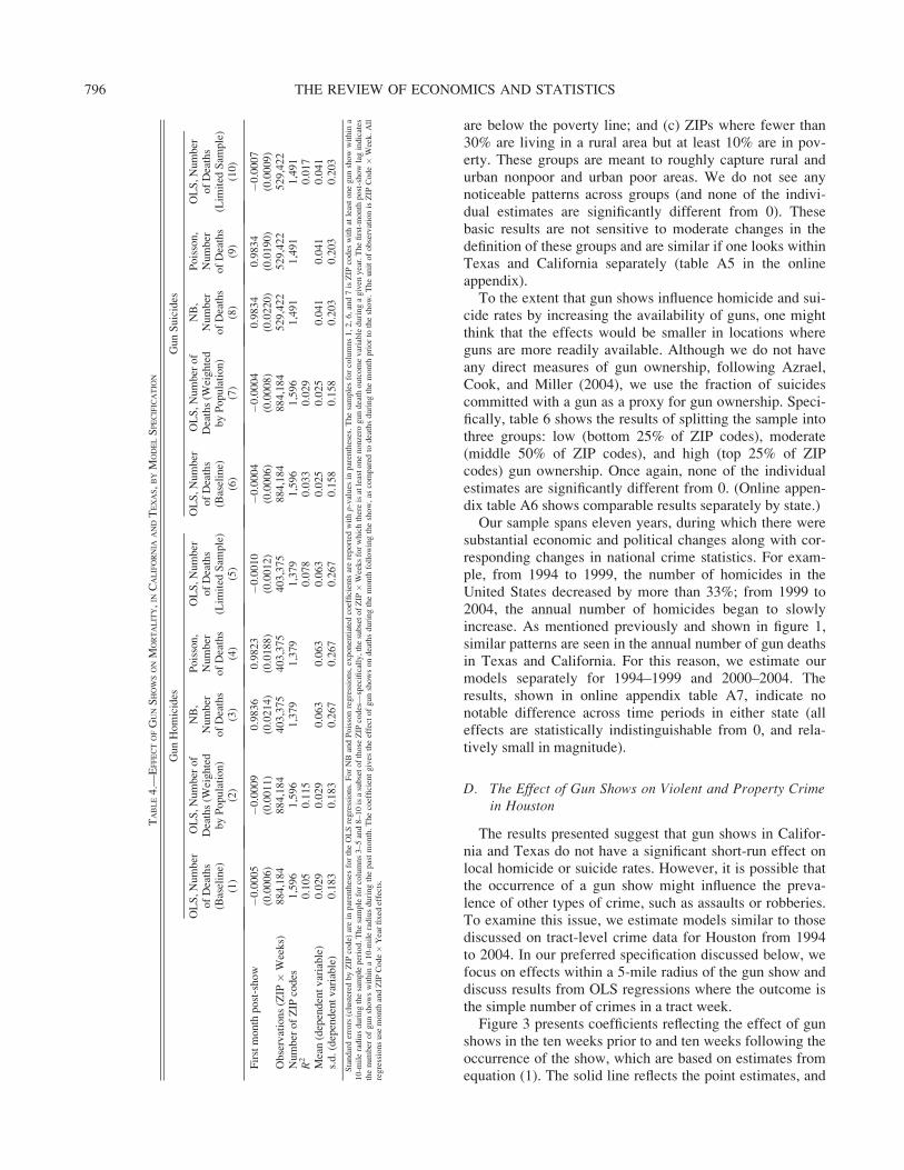
B. Sensitivity of Mortality Results

Table 4 explores whether the results above are sensitiveto the model specification. Column 1 reproduces the base-line results for gun homicides (table 2, panel C, column 1).Column 2 shows estimates that are weighted by the totalpopulation in the ZIP code (from the 2000 Census). Theresults are extremely similar to the unweighted estimates.Columns 3 and 4 show the exponentiated coefficients (and

p-values in parentheses) from negative binomial and Pois-son regressions where the outcome is the number of deaths.The sample sizes for these regressions are smaller than thebaseline because these models are estimated off the set ofobservations for which there is at least one gun death in agiven ZIP Code ! Year. Column 5 shows the OLS esti-mates for this same sample to allow one to distinguishbetween differences due to sample size and those due tomodel specification. Columns 6 through 10 present parallelspecifications for gun suicides. The basic pattern ofresults—both magnitude and significance—is comparableacross specifications for homicides and suicides. (Table A3in the online appendix shows these results separately bystate.)28

FIGURE 2.—EFFECT OF GUN SHOWS ON HOMICIDES AND SUICIDES IN CALIFORNIA AND TEXAS

Estimates come from the specification shown in equation (1) in the text. Rather than a one-month lag variable, however, there are ten lag and lead variables that indicate the number of deaths in the ZIP code duringthat week. Week 0 indicates the week of the gun show. The sample is all ZIP codes in California and Texas that have at least one gun show within a 10-mile radius during the sample period.

28 Online appendix table A8 shows results separately by ZIP code popu-lation. Consistent with the similarity of weighted and unweighted resultsin table 4, we find no significant patterns by ZIP code population size.

794 THE REVIEW OF ECONOMICS AND STATISTICS

In our baseline specification, we include ZIP Code !Year and month fixed effects. In the online appendix (tableA4), we present results from three alternative sets of fixedeffects: separate main effects for month, year, and ZIPcode; separate main effects for week defined over the entiresample period (1–573) and ZIP code; and week of year (1–52) and ZIP Code ! Year. The results do not change appre-ciably across any of these alternative specifications.

C. Heterogeneous Effects

Table 5 reports estimates of our baseline specification byZIP code characteristics. To explore whether the effect ofgun shows differs by poverty and urbanicity, we presentestimates for three mutually exclusive ZIP code categories:(a) ZIPs in which at least 30% of the population is living ina rural area (as defined by the census); (b) ZIPs in whichless than 30% are living in a rural area and fewer than 10%

TABLE 2.—EFFECT OF GUN SHOWS ON MORTALITY, BY GEOGRAPHICAL DISTANCE FOR CALIFORNIA AND TEXAS

A: Within ZIP Code B: Within 5-Mile Radius

Homicides Suicides Homicides SuicidesGun Nongun Gun Nongun Gun Nongun Gun Nongun(1) (2) (3) (4) (5) (6) (7) (8)

First month post-show 0.0014 0.0013 0.0018 #0.0019 #0.0001 0.0011* 0.0001 #0.0014(0.0027) (0.0015) (0.0024) (0.0025) (0.0011) (0.0007) (0.0009) (0.0009)

Observations (ZIP !Weeks) 120,772 120,772 120,772 120,772 463,144 463,144 463,144 463,144Number of ZIP codes 218 218 218 218 836 836 836 836R2 0.056 0.027 0.032 0.033 0.101 0.032 0.032 0.034Mean (dependent variable) 0.022 0.013 0.031 0.025 0.032 0.014 0.027 0.026s.d. (dependent variable) 0.159 0.119 0.178 0.159 0.194 0.122 0.167 0.162

C: Within 10-Mile Radius D: Within 25-Mile Radius

Homicides Suicides Homicides SuicidesGun Nongun Gun Nongun Gun Nongun Gun Nongun(9) (10) (11) (12) (13) (14) (15) (16)

First month post-show #0.0005 #0.0002 #0.0004 #0.0004 #0.0001 0.0001 #0.0003 #0.0003(0.0006) (0.0004) (0.0006) (0.0005) (0.0003) (0.0002) (0.0003) (0.0003)

Observations (ZIP !Weeks) 884,184 884,184 884,184 884,184 1,550,646 1,550,646 1,550,646 1,550,646Number of ZIP codes 1,596 1,596 1,596 1,596 2,799 2,799 2,799 2,799R2 0.105 0.033 0.033 0.035 0.104 0.034 0.036 0.038Mean (dependent variable) 0.029 0.012 0.025 0.023 0.019 0.008 0.019 0.016s.d. (dependent variable) 0.183 0.113 0.158 0.157 0.148 0.093 0.137 0.132

The sample for panel A is ZIP codes that have at least one gun show during the sample period. For panels, B, C, and D, it is ZIP codes with at least one gun show within a 5-, 10-, and 25-mile radius, respectively,during the sample period. The first-month post-show lag indicates the number of gun shows during the past month within ZIP code and within a 5-, 10-, or 25-mile radius for the respective samples. The coefficientgives the effect of gun shows on deaths during the month following the show, as compared to deaths during the month prior to the show. The unit of observation is ZIP Code ! Week. Standard errors (in parenthesis)are clustered by ZIP code. Uses Month and ZIP Code ! Year Fixed Effects. *Significant at 10%.

TABLE 3.—EFFECT OF GUN SHOWS ON MORTALITY WITHIN A 10-MILE RADIUS, BY STATE

Homicides Suicides

Gun Nongun Gun Nongun(1) (2) (3) (4)

CaliforniaFirst month post-show 0.0002 0.0001 0.0005 #0.0001

(0.0009) (0.0006) (0.0008) (0.0009)Observations (ZIP !Weeks) 499,154 499,154 499,154 499,154Number of ZIP Codes 901 901 901 901R2 0.120 0.034 0.033 0.034Mean (dependent variable) 0.035 0.013 0.025 0.028s.d. (dependent variable) 0.203 0.117 0.159 0.176

TexasFirst month post-show #0.0010 #0.0004 #0.0011 #0.0006

(0.0009) (0.0006) (0.0008) (0.0006)Observations (ZIP !Weeks) 385,030 385,030 385,030 385,030Number of ZIP Codes 695 695 695 695R2 0.065 0.032 0.033 0.030Mean (dependent variable) 0.021 0.011 0.024 0.016s.d. (dependent variable) 0.153 0.108 0.157 0.127

The sample for columns 1–4 is ZIP codes that have at least one gun show within a 10-mile radius during the sample period. The first-month post-show lag indicates the number of gun shows during the past monthwithin a 10-mile radius. The coefficient gives the effect of gun shows on deaths during the month following the show, as compared to deaths during the month prior to the show. The unit of observation is ZIP Code !Week. Standard errors (in parentheses) are clustered by ZIP code. Uses month and ZIP Code! Year fixed effects.

795SHORT-TERM AND LOCALIZED EFFECT OF GUN SHOWS

are below the poverty line; and (c) ZIPs where fewer than30% are living in a rural area but at least 10% are in pov-erty. These groups are meant to roughly capture rural andurban nonpoor and urban poor areas. We do not see anynoticeable patterns across groups (and none of the indivi-dual estimates are significantly different from 0). Thesebasic results are not sensitive to moderate changes in thedefinition of these groups and are similar if one looks withinTexas and California separately (table A5 in the onlineappendix).

To the extent that gun shows influence homicide and sui-cide rates by increasing the availability of guns, one mightthink that the effects would be smaller in locations whereguns are more readily available. Although we do not haveany direct measures of gun ownership, following Azrael,Cook, and Miller (2004), we use the fraction of suicidescommitted with a gun as a proxy for gun ownership. Speci-fically, table 6 shows the results of splitting the sample intothree groups: low (bottom 25% of ZIP codes), moderate(middle 50% of ZIP codes), and high (top 25% of ZIPcodes) gun ownership. Once again, none of the individualestimates are significantly different from 0. (Online appen-dix table A6 shows comparable results separately by state.)

Our sample spans eleven years, during which there weresubstantial economic and political changes along with cor-responding changes in national crime statistics. For exam-ple, from 1994 to 1999, the number of homicides in theUnited States decreased by more than 33%; from 1999 to2004, the annual number of homicides began to slowlyincrease. As mentioned previously and shown in figure 1,similar patterns are seen in the annual number of gun deathsin Texas and California. For this reason, we estimate ourmodels separately for 1994–1999 and 2000–2004. Theresults, shown in online appendix table A7, indicate nonotable difference across time periods in either state (alleffects are statistically indistinguishable from 0, and rela-tively small in magnitude).

D. The Effect of Gun Shows on Violent and Property Crimein Houston

The results presented suggest that gun shows in Califor-nia and Texas do not have a significant short-run effect onlocal homicide or suicide rates. However, it is possible thatthe occurrence of a gun show might influence the preva-lence of other types of crime, such as assaults or robberies.To examine this issue, we estimate models similar to thosediscussed on tract-level crime data for Houston from 1994to 2004. In our preferred specification discussed below, wefocus on effects within a 5-mile radius of the gun show anddiscuss results from OLS regressions where the outcome isthe simple number of crimes in a tract week.

Figure 3 presents coefficients reflecting the effect of gunshows in the ten weeks prior to and ten weeks following theoccurrence of the show, which are based on estimates fromequation (1). The solid line reflects the point estimates, and

TABLE4.—

EFFECTOFG

UNSHOWSONM

ORTALITY,I

NCALIFORNIA

ANDTEXAS,B

YM

ODELSPECIFICATIO

N

GunHomicides

GunSuicides

OLS,N

umber

ofDeaths

(Baseline)

OLS,N

umber

of

Deaths(W

eighted

byPopulation)

NB,

Number

ofDeaths

Poisson,

Number

ofDeaths

OLS,Number

ofDeaths

(Lim

ited

Sam

ple)

OLS,N

umber

ofDeaths

(Baseline)

OLS,N

umber

of

Deaths(W

eighted

byPopulation)

NB,

Number

ofDeaths

Poisson,

Number

ofDeaths

OLS,N

umber

ofDeaths

(Lim

ited

Sam

ple)

(1)

(2)

(3)

(4)

(5)

(6)

(7)

(8)

(9)

(10)

Firstmonth

post-show

#0.0005

#0.0009

0.9836

0.9823

#0.0010

#0.0004

#0.0004

0.9834

0.9834

#0.0007

(0.0006)

(0.0011)

(0.0214)

(0.0188)

(0.0012)

(0.0006)

(0.0008)

(0.0220)

(0.0190)

(0.0009)

Observations(ZIP

!Weeks)

884,184

884,184

403,375

403,375

403,375

884,184

884,184

529,422

529,422

529,422

Number

ofZIP

codes

1,596

1,596

1,379

1,379

1,379

1,596

1,596

1,491

1,491

1,491

R2

0.105

0.115

0.078

0.033

0.029

0.017

Mean(dependentvariable)

0.029

0.029

0.063

0.063

0.063

0.025

0.025

0.041

0.041

0.041

s.d.(dependentvariable)

0.183

0.183

0.267

0.267

0.267

0.158

0.158

0.203

0.203

0.203

Standarderrors(clustered

byZIP

code)

arein

parentheses

fortheOLSregressions.ForNBandPoissonregressions,exponentiated

coefficientsarereported

withp-values

inparentheses.Thesamplesforcolumns1,2,6,and7isZIP

codes

withat

leastonegunshowwithin

a10-m

ileradiusduringthesampleperiod.T

hesampleforcolumns3–5and8–10

isasubsetofthose

ZIP

codes—specifically,thesubsetofZIP

!Weeksforwhichthereisatleastonenonzerogundeath

outcomevariableduringagiven

year.Thefirst-month

post-showlagindicates

thenumber

ofgunshowswithin

a10-m

ileradiusduringthepastmonth.Thecoefficientgives

theeffect

ofgunshowsondeathsduringthemonth

followingtheshow,as

comparedto

deathsduringthemonth

priorto

theshow.TheunitofobservationisZIP

Code!

Week.All

regressionsuse

month

andZIP

Code!

Yearfixed

effects.

796 THE REVIEW OF ECONOMICS AND STATISTICS

the dashed line reflects the corresponding 95% confidenceband. Looking across the figures for gun violent crimes(panel A), nongun violent crimes (panel B), and propertycrimes (panel C), we see no evidence that gun shows influ-ence the prevalence of any type of crime. With regard togun violent crimes, the point estimates bounce around 0,never exceeding 0.02, and the 95% confidence interval formost weeks is between #0.02 and 0.02. Given that thenumber of gun violent crimes in the average tract-week

observation is 0.386, this suggests we can rule out effectslarger than 6%. For nongun violent and property crimes,our estimates rule out effects larger than 2% and 1%,respectively.

To more precisely and parsimoniously summarize theseresults, table 7 reports estimates of crime effects from equa-tion (2), which describes the impact of a gun show on crimein the four-week period following the show relative to thefour-week period preceding the show. None of the estimates

TABLE 5.—EFFECT OF GUN SHOWS ON MORTALITY IN CALIFORNIA AND TEXAS, BY POVERTY AND URBANICITY

Gun Homicides Gun Suicides

Rural Urban Nonpoor Urban Poor Rural Urban Nonpoor Urban Poor(1) (2) (3) (4) (5) (6)

First month post-show 0.0002 #0.0002 #0.0008 #0.0019 0.0009 #0.0011(0.0008) (0.0006) (0.0010) (0.0014) (0.0009) (0.0008)

Observations (ZIP ! Weeks) 142,378 298,606 443,200 142,378 298,606 443,200Number of ZIP codes 257 539 800 257 539 800R2 0.026 0.033 0.103 0.035 0.030 0.032Mean (dependent variable) 0.003 0.011 0.049 0.011 0.026 0.028s.d. (dependent variable) 0.061 0.108 0.238 0.105 0.161 0.170

Nongun Homicides Nongun Suicides

Rural Urban Nonpoor Urban Poor Rural Urban Nonpoor Urban Poor

First month post-show 0.0001 0.0001 #0.0004 #0.0008 0.0003 #0.0007(0.0006) (0.0005) (0.0006) (0.0011) (0.0009) (0.0007)

Observations (ZIP ! Weeks) 142,378 298,606 443,200 142,378 298,606 443,200Number of ZIP codes 257 539 800 257 539 800R2 0.024 0.023 0.031 0.029 0.029 0.035Mean (dependent variable) 0.002 0.006 0.019 0.006 0.025 0.027s.d. (dependent variable) 0.048 0.084 0.141 0.076 0.170 0.166

The sample is ZIP codes that have at least one gun show within a 10-mile radius during the sample period. Rural is defined as at least 30% rural as defined by the Census. Urban nonpoor is defined as less than 30%rural and less than 10% of percent of population below the poverty line. Urban poor is defined as less than 30% rural and at least 10% of population above the povery line. The first-month post-show lag indicates thenumber of gun shows within a 10-mile radius during the past month. The coefficient gives the effect of gun shows on deaths during the month following the show, as compared to deaths during the month prior to theshow. Standard errors (in parentheses) are clustered by ZIP code. The unit of observation is ZIP Code ! Week. Uses month and ZIP Code ! Year fixed effects.

TABLE 6.—EFFECT OF GUN SHOWS ON MORTALITY IN TEXAS AND CALIFORNIA, BY GUN OWNERSHIP

Low GunOwnership

Gun Homicidesand ModerateGun Ownership

High GunOwnership

Low GunOwnership

Gun Suicidesand ModerateGun Ownership

High GunOwnership

(1) (2) (3) (4) (5) (6)

First month post-show 0.0007 #0.0003 #0.0022 #0.0005 0.0002 #0.0018(0.0012) (0.0008) (0.0018) (0.0009) (0.0008) (0.0015)

Observations (ZIP !Weeks) 216,060 434,336 204,426 216,060 434,336 204,426Number of ZIP codes 390 784 369 390 784 369R2 0.099 0.108 0.089 0.031 0.029 0.035Mean (dependent variable) 0.025 0.036 0.020 0.015 0.031 0.025s.d. (dependent variable) 0.170 0.206 0.153 0.125 0.177 0.160

Nongun Homicides Nongun SuicidesLow GunOwnership

Moderate GunOwnership

High GunOwnership

Low GunOwnership

Moderate GunOwnership

High GunOwnership

First month post-show 0.0000 #0.0004 0.0000 0.0010 #0.0012 #0.0001(0.0008) (0.0005) (0.0009) (0.0011) (0.0008) (0.0008)

Observations (ZIP !Weeks) 216,060 434,336 204,426 216,060 434,336 204,426Number of ZIP codes 390 784 369 390 784 369R2 0.034 0.032 0.032 0.037 0.029 0.028Mean (dependent variable) 0.012 0.014 0.009 0.030 0.027 0.010s.d. (dependent variable) 0.113 0.124 0.097 0.191 0.165 0.099

The sample is ZIP codes that have at least one gun show within a 10-mile radius and one suicide during the sample period. The first-month post-show lag indicates the number of gun shows within a 10-mile radiusduring the past month. The coefficient gives the effect of gun shows on deaths during the month following the show, as compared to deaths during the month prior to the show. Fraction of suicides committed with agun is used to proxy gun ownership. Low gun ownership is defined as the bottom 25% of California and Texas ZIP codes; moderate is the middle 50%; and high is the top 25%. Standard errors (in parentheses) areclustered by ZIP code. The unit of observation is ZIP Code !Week. Uses month and ZIP Code ! Year fixed effects.

797SHORT-TERM AND LOCALIZED EFFECT OF GUN SHOWS

are statistically different than zero, and all are relativelyprecise. For example, given that the average number of gunviolent crimes within a tract-week observation in Houstonduring this period is 0.386, our estimates imply that we canrule out effects larger than 1.5% of the mean. The estimatesfor nongun violent and property crimes are even smaller inrelative magnitude and equally insignificant.

In results available in the online appendix, we show thatthe general conclusion of no effect is robust to negativebinomial, Poisson and population-weighted OLS estimates(table A9), to specifications that include alternative controlsfor time and location (table A10), and to alternate choicesof geographical proximity to a gun show (table A11).Finally, in results not reported but available on request, wedemonstrate that gun shows have no effect on more finelygrained crime categories including robberies, burglaries,motor vehicle thefts, assaults, and rapes. In summary, itappears that the occurrence of a gun show does not signifi-cantly affect short-run crime rates in localized areas.

VI. Conclusion

Thousands of gun shows take place in the United Statesevery year. Gun control advocates argue that the gun showloophole that exists in many states makes it easier for poten-tial criminals to obtain a gun. Gun shows may also affectsuicide rates by increasing the ease with which individualswho are contemplating suicide can obtain a more lethaldevice. Opponents of gun show regulations argue that gunshows are innocuous because potential criminals and otherindividuals can acquire guns easily through other channels.

In this paper, we have investigated the effect of gunshows using eleven years of data on the date and location ofevery gun show in California and Texas, the nation’s twomost populous states. To study the effect on mortality(homicide and suicide, in particular), we have combinedthis with information on the date, location, and cause ofevery death occurring in these same two states during oureleven-year study period. To study the effect of gun showson violent and property crime, we combine the gun showdata with crime data provided by the Houston PoliceDepartment from 1994 to 2004.

TABLE 7.—EFFECT OF GUN SHOWS ON CRIME IN HOUSTON, TEXAS

NongunViolentCrimes

GunViolentCrimes

PropertyCrimes

First month post-show #0.0089 #0.0040 #0.0121(0.0080) (0.0052) (0.0199)

Observations (Tract !Weeks) 122,434 122,434 122,434Number of census tracts 221 221 221R2 0.311 0.193 0.735Mean (dependent variable) 1.063 0.386 5.085s.d. (dependent variable) 1.416 0.768 5.090

The sample is census tracts that have at least one gun show within a 5-mile radius during the sampleperiod. The first-month post-show lag indicates the number of gun shows within a 5-mile radius duringthe past month. The coefficient gives the effect of gun shows on crimes during the month following theshow, as compared to crimes during the month prior to the show. The unit of observation is Census Tract !Week. Standard errors (in parentheses) are clustered by census tract. Uses month and Census Tract !Year Fixed Effects.

FIGURE 3.—EFFECT OF GUN SHOWS ON CRIME IN HOUSTON

Estimates come from the specification shown in equation (1) in the text. Rather than a one-month lagvariable, however, there are ten lag and lead variables that indicate the number of crimes in the censustract during that week. Week 0 indicates the week of the gun show. The sample is all census tracts inHouston that have at least one gun show within a 5-mile radius during the sample period.

798 THE REVIEW OF ECONOMICS AND STATISTICS

Using both event study techniques and specifications thatestimate the difference in mortality in the four weeks fol-lowing a gun show relative to the four weeks preceding ashow, we find no evidence that gun shows have an effect onany of our outcome measures: gun and nongun homicides,gun and nongun suicides, gun and nongun violent crimes,and property crime. In addition, the mortality results are thesame in both Texas and California, despite the fact thatCalifornia arguably has the strictest gun show regulationswhile Texas’s regulations are among the least stringent.Thus, our results suggest that gun shows do not increase thenumber of homicides or suicides and that the absence ofgun show regulations does not increase the number of gun-related deaths as proponents of these regulations suggest.There are, however, two important caveats to our ana-

lyses. First, we are considering only the effect in the geo-graphical area immediately surrounding gun shows. To theextent that firearms purchased at gun shows are transportedmore than 25 miles away from the show, our identificationstrategy will not capture this effect. In addition, we considerthe effect only in the four weeks immediately following agun show. However, guns are durable, and thus to theextent that effects occur much later, our analysis will notcapture this.

REFERENCES

Allison, Paul D., and Richard P. Waterman, ‘‘Fixed-Effects NegativeBinomial Regression Models,’’ Sociological Methodology 32,(2002), 247–265.

Ayres, I., and J. Donohue, ‘‘Nondiscretionary Concealed Weapons Law:A Case Study of Statistics, Standards of Proof, and Public Policy,’’American Law and Economics Review 1 (1999), 436–470.

Azrael, D., P. Cook, and M. Miller, ‘‘State and Local Prevalence of Fire-arms Ownership Measurement, Structure, and Trends,’’ Journal ofQuantitative Criminology 20 (2004), 43–62.

Azrael, D., D. Hemenway, and M. Miller, ‘‘Household Firearm Owner-ship and Suicide Rates in the United States,’’ Epidemiology 13(2002), 517–524.

Black, D., & D. Nagin, ‘‘Do Right-to-Carry Laws Deter Violent Crime?’’Journal of Legal Studies 27 (1998), 209–219.

Bollen, Kenneth, and David Phillips, ‘‘Imitative Suicides: A NationalStudy of the Effects of Television News Stories,’’ American Socio-logical Review 47 (1982), 802–809.

Bowling, Michael, Gene Lauver, Matthew Hickman, and Devon Adams,‘‘Background Checks for Firearm Transfers, 2005,’’ Bureau of Jus-tice Statistics Bulletin, 214256 (2006).

Cook, P. J., and J. Ludwig, Guns in America: Results of a ComprehensiveSurvey of Gun Ownership and Use (Washington, DC: Police Foun-dation, 1996).

——— ‘‘The Social Costs of Gun Ownership,’’ NBER working paper no.W10736 (2004).

Duggan, M., ‘‘More Guns, More Crime,’’ Journal of Political Economy109 (2001), 1086–2114.

Harlow, C., Firearm Use by Offenders (Washington, DC: Bureau of Jus-tice Statistics, U.S. Department of Justice, 2001).

Hausman, J., B. H. Hall, and Z. Griliches, ‘‘Econometric Models forCount Data with an Application to the Patents-R&D Relation-ship,’’ Econometrica 52 (1984), 909–938.

Kellermann, A., F. Rivara, G. Somes, G. Reay, J. Francisco, J. Banton, J.Prodzinski, C. Fligner, and B. Hackman, ‘‘Suicide in the Home inRelation to Gun Ownership,’’ New England Journal of Medicine327 (1992), 467–472.

Krouse, W., Gun Legislation in the 109th Congress. CongressionalResearch Service report RL32842 (March 31, 2005).

Legal Community against Violence, ‘‘Regulating Guns in America: AnEvaluation and Comparative Analysis of Federal, State andSelected Local Gun Laws,’’ http://www.lcav.org (2008).

Lott, J., The Bias against Guns (Washington, DC: Regnery, 2003).Lott, J., and D. Mustard, ‘‘Crime, Deterrence, and Right-to-Carry Con-

cealed Handguns,’’ Journal of Legal Studies 26 (1997) 1–68.Moody, C., ‘‘Testing for the Effects of Concealed Weapons Laws: Speci-

fication Errors and Robustness,’’ Journal of Law and Economics44: 2, Part 2 (2001), 799–813.

Obmascik, Mark, Marilyn Robinson, and David Olinger, ‘‘Officials SayGirlfriend Bought Guns,’’ Denver Post (April 27, 1999).

Office of Statistics and Programming, National Center for Injury Preven-tion and Control, CDC. WISQARS Injury Mortality Reports (1999–2006), http://webapp.cdc.gov/sasweb/ncipc/mortrate10_sy.html.Accessed August 3, 2009.

Sloan, J., F. Rivara, D. Reay, J. Ferris, M. Path, and A. Kellermann,‘‘Firearm Regulations and Rates of Suicide: A Comparison of TwoMetropolitan Areas,’’ New England Journal of Medicine 322(1990), 369–373.

U.S. Department of Justice, ‘‘The Bureau of Alcohol, Tobacco, Firearms,and Explosives’ Investigative Operations at Gun Shows,’’ http://www.usdoj.gov/oig/reports/ATF/e0707/final.pdf (2007). AccessedAugust 4, 2009.

U.S. Department of Justice, Bureau of Justice Statistics, Survey of StateProcedures Related to Firearm Sales, Midyear 2002 (Washington,DC, October 15, 2003).

U.S. Department of Justice and U.S. Department of the Treasury, Bureauof Alcohol, Tobacco and Firearms, Gun Shows: Brady Checks andCrime Gun Traces, http://www.treas.gov/press/releases/report3100(January 1999). Accessed May 23, 2005.

U.S. Department of the Treasury, Bureau of Alcohol, Tobacco and Fire-arms, Following the Gun: Enforcing Federal Laws against Fire-arms Traffickers, http://www.atf.gov (June 2000). Accessed May31, 2005.

U.S. Department of the Treasury, Bureau of Alcohol, Tobacco and Fire-arms, Annual Firearms Manufacturers and Export Report, http://www.atf.gov (2006). Accessed August 12, 2008.

Virginia Tech Review Panel, Mass Shootings at Virginia Tech, Report ofthe Virginia Tech Review Panel presented to Governor KaineCommonwealth of Virginia, http://www.governor.virginia.gov/TempContent/techPanelReport.cfm (2007). Accessed August 13,2008.

Wintemute, G., ‘‘Gun Shows across a Multistate American Gun Market:Observational Evidence of the Effects of Regulatory Policy,’’Injury Prevention 13 (2007), 150–155.

799SHORT-TERM AND LOCALIZED EFFECT OF GUN SHOWS

This article has been cited by:

1. Matthew Lang. 2016. State Firearm Sales and Criminal Activity: Evidence from Firearm Background Checks. Southern EconomicJournal n/a-n/a. [CrossRef]

2. Emilio Depetris-Chauvin. 2015. Fear of Obama: An empirical study of the demand for guns and the U.S. 2008 presidential election.Journal of Public Economics 130, 66-79. [CrossRef]

3. JASON M. LINDO, CHARLES STOECKER. 2014. DRAWN INTO VIOLENCE: EVIDENCE ON “WHAT MAKES ACRIMINAL” FROM THE VIETNAM DRAFT LOTTERIES. Economic Inquiry 52:10.1111/ecin.2014.52.issue-1, 239-258.[CrossRef]

4. Christopher G. KopackiFirearms 1-7. [CrossRef]5. ARINDRAJIT DUBE, OEINDRILA DUBE, OMAR GARCÍA-PONCE. 2013. Cross-Border Spillover: U.S. Gun Laws and Violence

in Mexico. American Political Science Review 107, 397-417. [CrossRef]