The Scale of the Cosmos - Los Angeles Mission College

Michael Seeds

Dana Backman

Chapter 9

The Family of Stars

[Love] is the star to

every wandering bark,

Whose worth’s unknown,

although his height be taken.

• WILLIAM SHAKESPEARE

Sonnet 116

• Shakespeare compared love to a star

that can be seen easily and even used

for guidance, but whose real nature is

utterly unknown.• He lived at about the same time as Galileo and had no

idea what stars actually are.

• To understand the history of the

universe, the origin of Earth, and the

nature of our human existence, you

need to discover what people in

Shakespeare’s time did not know:• The real nature of the stars

• Unfortunately, it is quite difficult to

find out what a star is like.• When you look at a star even through a telescope,

you see only a point of light.

• Real understanding of stars requires careful analysis

of starlight.

• This chapter concentrates on

five goals:• Knowing how far away stars are

• How much energy they emit

• What their surface temperatures are

• How big they are

• How much mass they contain

Star Distances

• Distance is the most important,

and the most difficult,

measurement in astronomy.

• Astronomers have many different

ways to find the distances to stars.• Each of those ways depends on a simple and direct

geometrical method that is much like the method

surveyors would use to measure the distance across a

river they cannot cross.

• You can begin by reviewing that method and then

apply it to stars.

Star Distances

• To measure the distance across a

river, a team of surveyors begins by

driving two stakes into the ground.• The distance between the stakes is called the baseline.

The Surveyor’s Triangulation Method

• Then, they choose a landmark on the

opposite side of the river, perhaps a tree.

• This establishes a large triangle marked

by the two stakes and the tree.• Using their instruments,

they sight the tree

from the two ends of

the baseline and measure

the two angles on

their side of the river.


• Then, they can find the distance

across the river by simple

trigonometry.• So, if the baseline is

50 meters and the angles

are 66° and 71°, they

would calculate that

the distance from the

baseline to the tree is

64 meters.


• To find the distance to a star,

astronomers use a very long

baseline:• The diameter of Earth’s orbit

The Astronomer’s Triangulation Method

• If you take a photo of a nearby star and then

wait six months, Earth will have moved

halfway around its orbit.

• You can then take another photo of the star

from a slightly different location in space.• When you examine the

photos, you will discover

that a star is not in exactly

the same place in the

two photos.


• You have learned that parallax is the term

that refers to the common experience of an

apparent shift in the position of a foreground

object due to a change in the location of the

observer’s viewpoint.• Your thumb, held at

arm’s length, appears

to shift position against

a distant background

when you look first

with one eye and then

with the other.


• The baseline is the distance between

your eyes.

• The parallax is the angle through which

your thumb appears to move when you

switch eyes.• The farther away

you hold your thumb,

the smaller the

parallax.


• As the stars are so distant, their parallaxes

are very small angles—usually expressed in

arc seconds.

• The quantity that astronomers call stellar

parallax (p) is defined as half the total shift

of the star.• In other words, it is

the shift seen across

a baseline of 1 AU

rather than 2 AU.


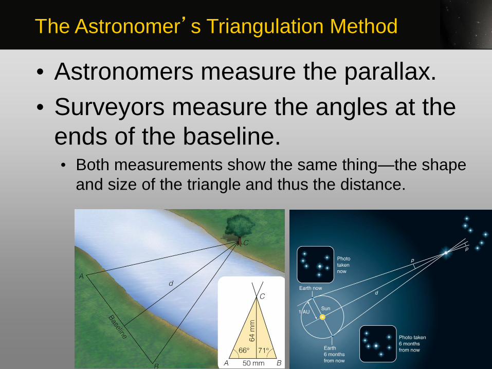
• Astronomers measure the parallax.

• Surveyors measure the angles at the

ends of the baseline.• Both measurements show the same thing—the shape

and size of the triangle and thus the distance.


• Measuring the parallax p is very

difficult because it is such a small

angle.• The nearest star, Alpha Centauri, has a parallax of

only 0.76 arc seconds.

• More distant stars have

even smaller parallaxes.


• To understand how small these

angles are, imagine a dime two

miles away from you.• That dime covers an angle

of about 1 arc second.


• Stellar parallaxes are so small that

the first successful measurement of

one did not happen until 1838—more

than 200 years after the invention of

the telescope.


• The distances to the stars are so large that

it is not convenient to use kilometers or

astronomical units.

• When you measure distance via parallax, it

is better to use the unit of distance called a

parsec (pc).• The word parsec was created by combining parallax

and arc second.


• One parsec equals the distance to

an imaginary star that has a parallax

of 1 arc second.

• A parsec is 206,265 AU—roughly

3.26 ly.


• Parsec units are used more often than

light-years by astronomers because

parsecs are more directly related to the

process of measurement of star distances.

• However, there are instances in which the light-

year is also useful.


• The blurring caused by Earth’s atmosphere

makes star images appear about 1 arc

second in diameter.

• That makes it difficult to measure parallax. • Even if you average together many observations made

from Earth’s surface, you cannot measure parallax with

an uncertainty smaller than about 0.002 arc seconds.

• Thus, if you measure a parallax of 0.006 arc seconds

from an observatory on the ground, your uncertainty will

be about 30 percent.


• If you consider—as astronomers generally

do—that 30 percent is the maximum

acceptable level of uncertainty, then

ground-based astronomers can’t measure

parallaxes accurately that are smaller than

about 0.006 arc seconds.

• That parallax corresponds to a distance of about

170 pc (550 ly).


• In 1989, the European Space Agency

launched the satellite Hipparcos to

measure stellar parallaxes from above

the blurring effects of Earth’s atmosphere.

• That small space telescope observed for

four years.


• The data were used to produce

two parallax catalogs in 1997.• One catalog contains 120,000 stars with parallaxes

20 times more accurate than ground-based

measurements.

• The other catalog contains over a million stars with

parallaxes as accurate as ground-based parallaxes.

• Knowing accurate distances from the Hipparcos

observations has given astronomers new insights

into the nature of stars.


• Your eyes tell you that some stars

look brighter than others.

• Also, you have learned about the

apparent magnitude scale that refers

to stellar apparent brightness.

Star Apparent Brightness, Intrinsic Brightness, and Luminosities

• However, the scale informs you only

how bright stars appear to you on

Earth.

• To know the true nature of a star, you

must know its intrinsic brightness.• This is a measure of the amount of energy the

star emits.


• An intrinsically very bright star might

appear faint if it is far away.

• Thus, to know the intrinsic brightness

of a star, you must take into account

its distance.


• When you look at a bright light, your

eyes respond to the visual-wavelength

energy falling on your retinas—which

tells you how bright the object appears.• Thus, brightness is related to the flux of energy entering

your eye.

Brightness and Distance

• Astronomers and physicists define

flux as the energy in Joules (J) per

second falling on 1 square meter.• A Joule is about the amount of energy released

when an apple falls from a table onto the floor.


• A flux of 1 Joule per second is also

known as 1 Watt.• The wattage of a light bulb gives you its intrinsic

brightness.

• Compare that with the apparent brightness of a light

bulb, which depends on its distance from you.


• If you placed a screen 1 m2 near a

light bulb, a certain amount of flux

would fall on the screen.


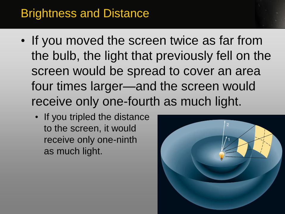
• If you moved the screen twice as far from

the bulb, the light that previously fell on the

screen would be spread to cover an area

four times larger—and the screen would

receive only one-fourth as much light. • If you tripled the distance

to the screen, it would

receive only one-ninth

as much light.


• Thus, the flux you receive from a light

source is inversely proportional to the

square of the distance to the source.

• This is known as the inverse square relation.


• Now you can understand how the

apparent brightness of a star

depends on its distance.• If astronomers know the apparent brightness of a

star and its distance from Earth, they can use the

inverse square law to correct for distance and find

the intrinsic brightness of the star.


• If all the stars were the same distance

away, you could compare one with

another and decide which was

intrinsically brighter or fainter.• Of course, the stars are scattered at different

distances, and you can’t move them around to line

them up for comparison.

Absolute Visual Magnitude

• If, however, you know the distance to

a star, you can use the inverse

square relation to calculate the

brightness the star would have at

some standard distance.


• Astronomers use 10 pc as the standard

distance.

• They refer to the intrinsic brightness of

the star as its absolute visual magnitude

(MV).• This is the apparent visual magnitude that the star

would have if it were 10 pc away.

• The subscript V informs you it is a visual magnitude—

referring to only the wavelengths of light your eye can

see.


• Other magnitude systems are based

on other parts of the electromagnetic

spectrum—such as infrared and

ultraviolet radiation.


• The sun’s absolute magnitude is

easy to calculate—because its

distance and apparent magnitude

are well known.• The absolute visual magnitude of the sun is about 4.8.

• In other words, if the sun were only 10 pc (33 ly) from

Earth, it would have an apparent magnitude of 4.8.

• It would look no brighter to your eye than the faintest

star in the handle of the Little Dipper.


• This path to find the distance to stars

has led you to absolute magnitude.

• You are now ready to reach the next

of your five goals in the chapter.


• The second goal for the

chapter is to find out how much

energy the stars emit.

Luminosity

• With the knowledge of the absolute

magnitudes of the stars, you can now

compare stars using our sun as a

standard.• The intrinsically brightest stars have absolute

magnitudes of about –8.

• This means that, if such a star were 10 pc away from

Earth, you would see it nearly as bright as the moon.

• Such stars emit over 100,000 times more visible light

than the sun.

Luminosity

• Absolute visual magnitude refers to

visible light.

• However, you want to know the total

output—including all types of radiation.• Hot stars emit a great deal of ultraviolet radiation that

you can’t see.

• Cool stars emit plenty of infrared radiation.

Luminosity

• To add in the energy you can’t see,

astronomers make a mathematical

correction that depends on the temperature

of the star.

• With that correction, they can find the total

electromagnetic energy output of a star.

• They refer to this as its luminosity (L).

Luminosity

• Astronomers know the luminosity of the

sun because they can send satellites

above Earth’s atmosphere and measure

the amount of energy arriving from the sun.

• Also, they add up radiation of every

wavelength, including the types blocked by

the atmosphere.

Luminosity

• Of course, they also know the

distance from Earth to the sun very

accurately—which is necessary to

calculate luminosity.• The luminosity of the sun is about 4x1026 Watts

(Joules per second).

Luminosity

• You can express a star’s

luminosity in two ways.• For example, you can say that the star Capella (Alpha

Aurigae) is 100 times more luminous than the sun.

• You can also express this in real energy units by

multiplying by the luminosity of the sun.

• The luminosity of Capella is 4x1028 Watts.

Luminosity

• When you look at the night sky, the

stars look much the same.

• Yet, your study of distances and

luminosities reveals an astonishing fact.• Some stars are almost a million times more luminous

than the sun, and some are almost a million times less

luminous.

• Clearly, the family of stars is filled with interesting

characters.

Luminosity

• Your third goal in the

chapter is to learn about the

temperatures of stars.

Star Temperatures

• The surprising fact is that stellar

spectral lines can be used as a

sensitive star thermometer.

Star Temperatures

• From the study of blackbody radiation, you

know that temperatures of stars can be

estimated from their color—red stars are

cool, and blue stars are hot.

• However, the relative strengths of various

spectral lines give much greater accuracy

in measuring star temperatures.

Spectral Lines and Temperature

• You have also learned that, for

stars, the term surface refers to

the photosphere.• This is the limit of our vision into the star from

outside.

• This is not, however, an actual solid surface.


• Stars typically have surface

temperatures of a few thousand or

tens of thousands of degrees Kelvin.• As you will discover later, the centers of stars are

much hotter than their surfaces—many millions of

degrees.

• The spectra, though, inform only about the outer

layers from which the light you see originates.


• As you have learned, hydrogen Balmer

absorption lines are produced by

hydrogen atoms with electrons initially in

the second energy level.


• The strength of these spectral lines can be

used to gauge the temperature of a star.

• This is because, from lab experiments with

gasses and radiation and also from

theoretical calculations, scientists know of

various things.


• One, if the surface of a star is as cool as the

sun or cooler, there are few violent collisions

between atoms to excite the electrons.

• Most atoms will have their electrons in the

ground (lowest) state.• These atoms can’t absorb photons in the Balmer series.

• Thus, you should expect to find weak hydrogen Balmer

absorption lines in the spectra of very cool stars.


• Two, in the surface layers of stars hotter

than about 20,000 K, there are many violent

collisions between atoms.

• These excite electrons to high energy levels

or knock the electrons completely out of

most atoms—so they become ionized. • In this case, few hydrogen atoms will have electrons in

the second energy level to form Balmer absorption lines.

• So, you should also find weak hydrogen Balmer

absorption lines in the spectra of very hot stars.


• Finally, at an intermediate temperature—

roughly 10,000 K—the collisions have the

correct amount of energy to excite large

numbers of electrons into the second

energy level. • With many atoms excited to the second level, the gas

absorbs Balmer wavelength photons well—producing

strong hydrogen Balmer lines.


• Thus, the strength of the hydrogen

Balmer lines depends on the

temperature of the star’s surface

layers.• Both hot and cool stars have weak Balmer lines.

• Medium-temperature stars have strong Balmer lines.


• The figure shows the relationship

between gas temperature and

strength of spectral lines for hydrogen

and other substances.


• Each type of atom or molecule produces

spectral lines that are weak at high and low

temperatures and strong at some

intermediate temperature.

• The temperature at which the lines reach

maximum strength

is different for

each type of atom

or molecule.


• Theoretical calculations of the type

first made by Cecilia Payne can

predict just how strong various

spectral lines should be for stars of

different temperatures.


• Astronomers can determine a star’s

temperature by comparing the

strengths of its spectral lines with the

predicted strengths.• From stellar spectra, astronomers have found that the

hottest stars have surface temperatures above 40,000 K

and the coolest about 2,000 K.

• Compare these with the surface temperature of the

sun—which is about 5,800 K.


• You have seen that the strengths of

spectral lines depend on the surface

(photosphere) temperature of the star.

• From this, you can predict that all stars of

a given temperature should have similar

spectra.

Temperature Spectral Classification

• Learning to recognize the pattern of

spectral lines produced in the atmospheres

of stars of different temperatures means

there is no need to do a full analysis every

time each type of spectrum is

encountered. • Time can be saved by classifying stellar spectra rather

than analyzing each spectrum individually.


• Astronomers classify stars by the

lines and bands in their spectra.• For example, if it has weak Balmer lines and lines of

ionized helium, it must be an O star.


• The star classification system now used by

astronomers was devised at Harvard during

the 1890s and 1900s.

• One of the astronomers there, Annie J.

Cannon, personally inspected and classified

the spectra of over 250,000 stars.


• The spectra were first classified in

groups labeled A through Q.

• Later, some groups were dropped,

merged with others, or reordered.


• The final classification includes

seven main spectral classes or types

that are still used today:• O, B, A, F, G, K, and M


• This set of star types—called the

spectral sequence—is important

because it is a temperature sequence.• The O stars are the hottest.

• The temperature continues to decrease down to

the M stars, the coolest.


• For further precision, astronomers

divide each spectral class into 10

subclasses.• For example, spectral class A consists of the

subclasses A0, A1, A2, . . . A8, and A9.

• Next come F0, F1, F2, and so on.


• These finer divisions define a

star’s temperature to a precision

of about 5 percent.• Thus, the sun is not just a G star.

• It is a G2 star, with a temperature of 5,800 K.


• Generations of astronomy students

have remembered the spectral

sequence by using various mnemonics.• Oh Boy, An F Grade Kills Me.

• Only Bad Astronomers Forget Generally Known

Mnemonics.


• Recently, astronomers have added

two more spectral classes—L and T.

• These represent objects cooler than

stars—called brown dwarfs.


• The figure shows color images of 13

stellar spectra—ranging from the hottest

at the top to the coolest at the bottom.


• Notice how spectral features change

gradually from hot to cool stars.


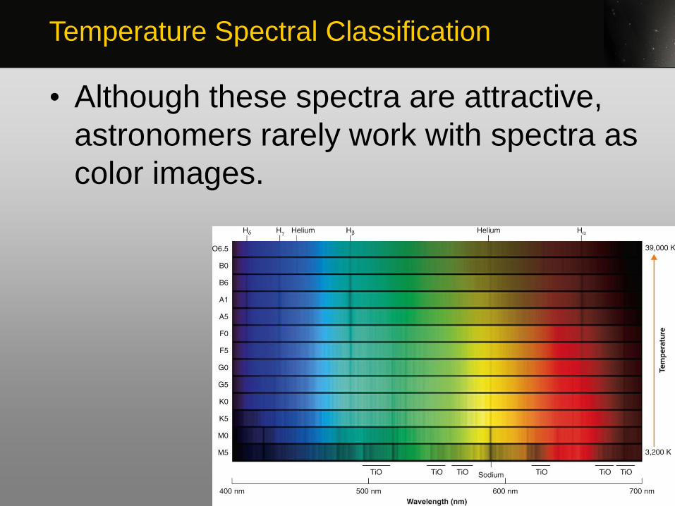
• Although these spectra are attractive,

astronomers rarely work with spectra as

color images.


• Rather, they display

spectra as graphs of

intensity versus

wavelength with dark

absorption lines as dips

in the graph.• Such graphs show more

detail than photos.


• Notice also that the

overall curves are

similar to blackbody

curves.

• The wavelength of

maximum is in the

infrared for the coolest

stars and in the

ultraviolet for the

hottest stars.


• Compare the figures

and notice how the

strength of spectral

lines depends on

temperature.


• Your fourth goal in the

chapter is to learn about the

sizes of stars.

Star Sizes

• Do stars all have the same

diameter as the sun, or are some

larger and some smaller?• You certainly can’t see their sizes through a telescope.

• The images of the stars are much too small for you to

resolve their disks and measure their diameters.

• There is a way, however, to find out how big stars really

are.

Star Sizes

• The luminosity of a glowing object like a

star is determined by its surface area

and temperature.• For example, you can eat dinner by candlelight because

the candle flame has a small surface area.

• Although it is very hot, it cannot radiate much heat

because it is small—it has a low luminosity.

Luminosity, Temperature, and Diameter

• However, if the candle flame were 12 feet

tall, it would have a very large surface area

from which to radiate.

• Although it might be the same temperatures

as a normal candle flame, its luminosity

would drive you from the table.


• Similarly, a star’s luminosity is

proportional to its surface area.• A hot star may not be very luminous if it has a small

surface area—but it could be highly luminous if it were

larger.

• Even a cool star could be luminous if it had a large

surface area.


• You can use stellar luminosities to

determine the diameters of stars—

if you can separate the effects of

temperature and surface area.


• The Hertzsprung-Russell (H-R)

diagram is a graph that separates the

effects of temperature and surface

area on stellar luminosities.• Thus, it enables astronomers to sort the stars

according to their diameters.


• The diagram is named after its

originators:• Ejnar Hertzsprung in the Netherlands

• Henry Norris Russell in the United States


• Before discussing the details of the H–R

diagram, look at a similar diagram you

might use to compare automobiles.• You can plot a diagram

to show horsepower

versus weight for

various makes of cars.


• You will find that, in general, the more

a car weighs, the more horsepower it

has.• Most cars fall somewhere

along the normal sequence

of cars running from heavy,

high-powered cars to

light, low-powered models.

• You might call this

the main sequence of cars.


• However, the sport or racing models have

much more horsepower than normal for

their weight.

• In contrast, the

economy models have

less power than normal

for cars of the same

weight.


• Just as this diagram helps you understand

the different kinds of autos, so the H-R

diagram can help you understand different

kinds of stars.


• An H-R diagram

has luminosity

on the vertical

axis and

temperature on

the horizontal

axis.• A star is

represented by a

point on the graph

that shows its

luminosity and

temperature.


• Note that, in

astronomy, the

symbol Θ refers

to the sun. • Thus, LΘ refers to

the luminosity of

the sun, TΘ refers

to the temperature

of the sun, and so

on.


• The diagram

also contains a

scale of spectral

types across

the top.


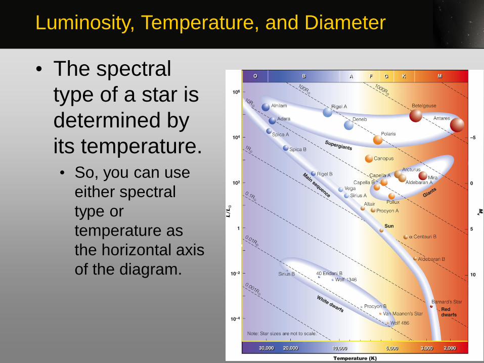
• The spectral

type of a star is

determined by

its temperature.• So, you can use

either spectral

type or

temperature as

the horizontal axis

of the diagram.


• Astronomers use H-R diagrams so often

that they usually skip the words “the point

that represents the star.”

• Rather, they will say that a star is located in

a certain place in the diagram. • Of course, they mean the point that represents the

luminosity and temperature of the star and not the star

itself.


• The location of a star in the H-R diagram

has nothing to do with the location of the

star in space.

• Furthermore, a star may move in the

diagram as it ages and its luminosity and

temperature change—but it has nothing to

do with the star’s motion.


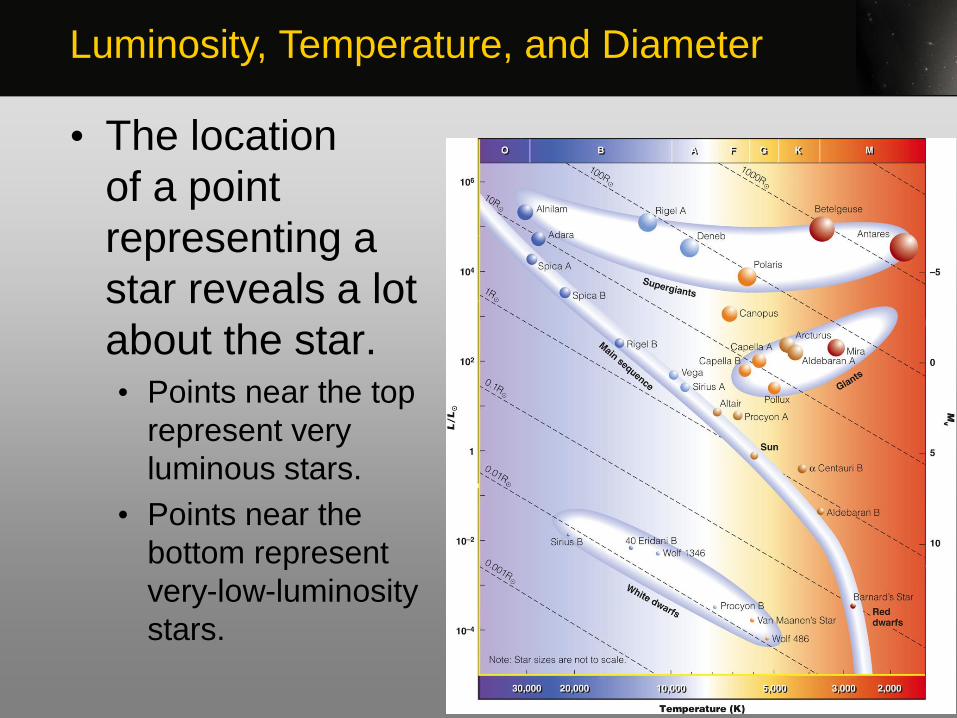
• The location

of a point

representing a

star reveals a lot

about the star.• Points near the top

represent very

luminous stars.

• Points near the

bottom represent

very-low-luminosity

stars.


• Also, points near the

right edge represent

very cool stars.

• Points near the left

edge represent very

hot stars.


• In this figure,

notice how color

has been used

to represent

temperature.• Cool stars are red.

• Hot stars are blue.


• The main

sequence is the

region of the

diagram running

from upper left

to lower right. • It includes roughly

90 percent of all

normal stars—

represented by a

curved line with

dots for stars

plotted along it.


• As you might

expect, the hot

main-sequence

stars are more

luminous than

the cool main-

sequence stars.


• In addition to temperature,

size is important in

determining the luminosity

of a star.


• Some cool stars

lie above the

main sequence.• Although they are

cool, they are

luminous.

• So, they must be

larger—have more

surface area—than

main-sequence

stars of the same

temperature.


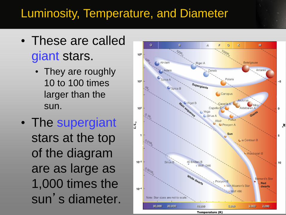
• These are called

giant stars.• They are roughly

10 to 100 times

larger than the

sun.

• The supergiant

stars at the top

of the diagram

are as large as

1,000 times the

sun’s diameter.


• In contrast, red

dwarfs at the

lower end of the

main sequence

are not only cool

but also small,

giving them low

luminosities.


• In contrast, the

white dwarfs lie

in the lower left

of the diagram.• Although some are

among the hottest

stars known, they

are so small they

have very little

surface area from

which to radiate.

• That limits them to

low luminosities.


• A simple calculation can be made to draw precise lines of constant radius across the diagram—based on the luminosities and temperatures at each point.


• For example,

locate the line

labeled 1RΘ

(1 solar radius).• Notice that it

passes through the

point representing

the sun.

• Any star whose

point is located

along this line has

a radius equal to

the sun’s radius.


• Notice also that

the lines of

constant radius

slope downward

to the right.• This is because

cooler stars are

always fainter than

hotter stars of the

same size,

following the

Stefan-Boltzman

Law.


• These lines of

constant radius

show

dramatically that

the supergiants

and giants are

much larger

than the sun.


• In contrast,

white dwarf

stars fall near

the line labeled

0.01 RΘ. • They all have

about the same

radius—

approximately the

size of Earth!


• Notice the great

range of sizes. • The largest stars

are 100,000 times

larger than the tiny

white dwarfs.

• If the sun were a

tennis ball, the

white dwarfs would

be grains of sand,

and the largest

supergiant stars

would be as big as

football fields.


• A star’s spectrum also contains clues

to whether it is a main-sequence star,

a giant, or a supergiant. • The larger a star is, the less dense

its atmosphere is.

Luminosity Spectral Classification

• The widths of spectral lines are

partially determined by the density

of the gas.• If the atoms collide often in a dense gas, their energy

levels become distorted, and the spectral lines are

broadened.


• In the spectrum of a main-sequence

star, the hydrogen Balmer lines are

broad.• The star’s atmosphere is dense and the hydrogen

atoms collide often.


• In the spectrum of a giant star, the

lines are narrower.• The giant star’s atmosphere is less dense and the

hydrogen atoms collide less often.


• In the spectrum of a supergiant

star, the lines are very narrow.


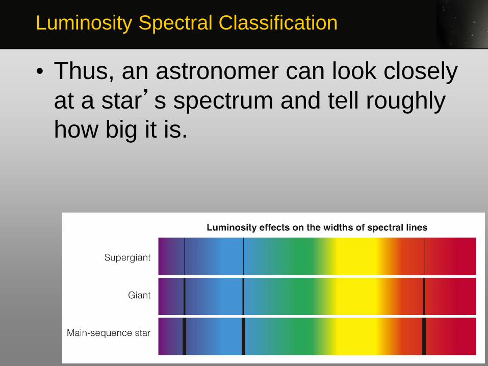
• Thus, an astronomer can look closely

at a star’s spectrum and tell roughly

how big it is.


• Size categories are called

luminosity classes—because the

size of the star is the dominating

factor in determining luminosity.• Supergiants, for example, are very luminous

because they are very large.


• The luminosity classes are

represented by the Roman numerals

I through V.• Adhara (Epsilon Canis Majoris) is a bright giant (II).

• Capella (Alpha Aurigae) is a giant (III).

• Altair (Alpha Aquilae) is a subgiant (IV).

• The sun is a main-sequence star (V).


• Supergiants are further subdivided

into types Ia and Ib.• For example, you can distinguish between a bright

supergiant (Ia) such as Rigel (Beta Orionis) and a

regular supergiant (Ib) such as Polaris, the North Star

(Alpha Ursa Minoris).


• The luminosity class notation

appears after the spectral

type—as in G2 V for the sun.


• White dwarfs don’t enter into

this classification.• Their spectra are very different from the other

types of stars.


• The

approximate

positions of the

main sequence,

giant, and

supergiant

luminosity

classes are

shown in this

H-R diagram.


• Luminosity classification is subtle and

not too accurate.

• Nevertheless, it is an important

technique because it provides clues to

distance.


• Most stars are too distant to have

measurable parallaxes.

• Nevertheless, astronomers can find the

distances to these stars—if they can

record the stars’ spectra and determine

their luminosity classes.


• From spectral type and luminosity class,

astronomers can estimate the star’s

absolute magnitude, compare with its

apparent magnitude, and compute its

distance.

• Although this process finds distance and

not true parallax, it is called spectroscopic

parallax.


• For example, consider

Betelgeuse (Alpha Orionis).• It is classified M2 Ia.

• Its apparent magnitude averages about 0.0

(Betelgeuse is somewhat variable).


• Plotting it in an H-R diagram, you will find that a temperature class of M2 and a luminosity class of Ib (supergiant) corresponds to a luminosity of about 30,000 LΘ.


• That information, combined with the star’s

apparent brightness, allows astronomers to

estimate that Betelgeuse is about 190 pc

from Earth.

• The Hipparcos satellite finds the actual

distance to be 131 pc.• So, the distance from the spectroscopic parallax

technique is only approximate.


• Spectroscopic parallax does give a

good first estimate of the distances of

stars so far away that their parallax

can’t easily be measured.


• Your fifth goal in the chapter is

to find out how much matter

stars contain—that is, to know

their masses.

Masses of Stars—Binary Stars

• Gravity is the key to determining

mass.• Matter produces a gravitational field.

• Astronomers can figure out how much matter a star

contains if they watch an object such as another star

move through the star’s gravitational field.


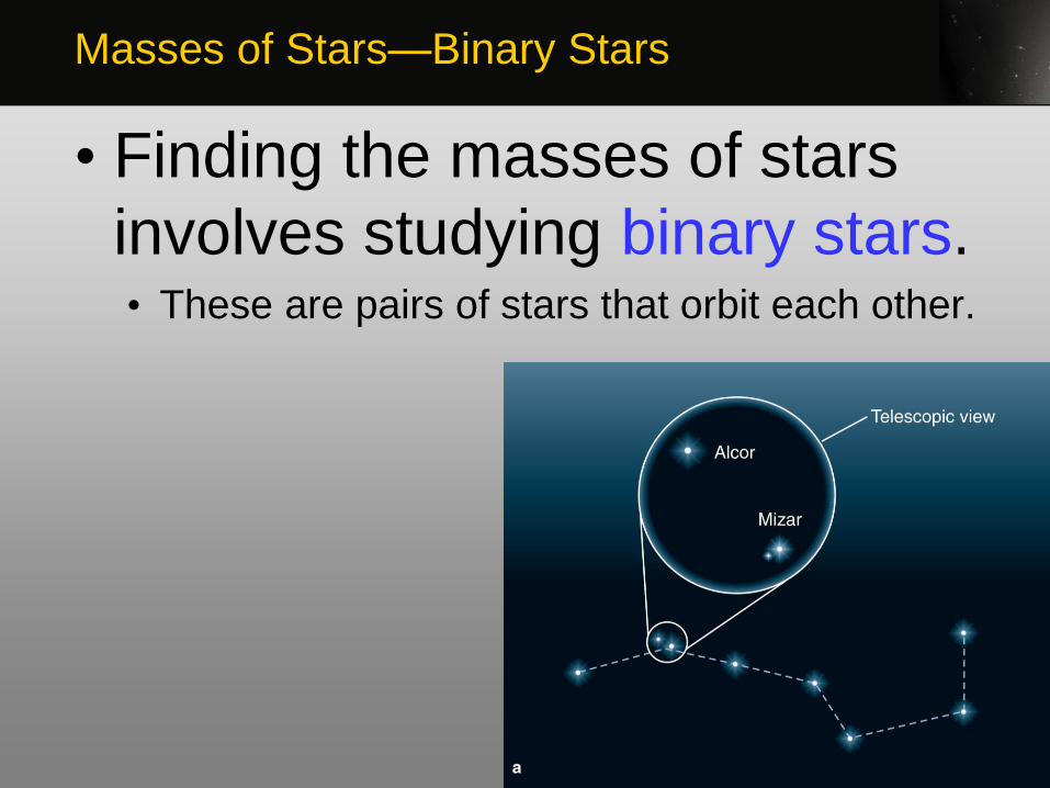
• Finding the masses of stars

involves studying binary stars.• These are pairs of stars that orbit each other.


• Many of the familiar stars in the

sky are actually pairs of stars

orbiting each other.• Binary systems are common.

• More than half of all stars are members of binary star

systems.


• Few, however, can be analyzed

completely.• Many are so far apart that their periods are much too

long for practical mapping of their orbits.

• Others are so close together they are not visible as

separate stars.


• The key to finding the mass of a

binary star is an understanding

of orbital motion.

Binary Stars in General

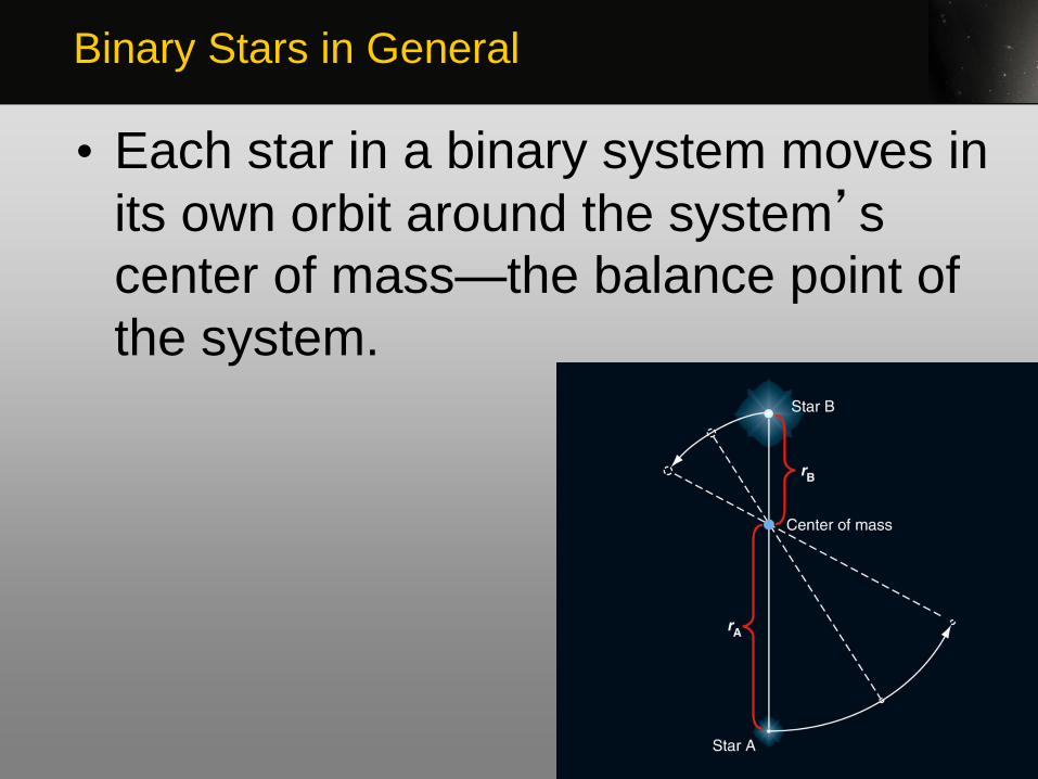
• Each star in a binary system moves in

its own orbit around the system’s

center of mass—the balance point of

the system.


• If one star is more massive than its

companion, then the massive star is closer

to the center of mass and travels in a

smaller orbit.

• In contrast,

the lower-mass star

whips around in

a larger orbit.


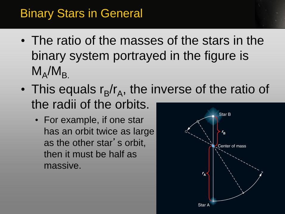
• The ratio of the masses of the stars in the

binary system portrayed in the figure is

MA/MB.

• This equals rB/rA, the inverse of the ratio of

the radii of the orbits. • For example, if one star

has an orbit twice as large

as the other star’s orbit,

then it must be half as

massive.


• Getting the ratio of the masses is

easy.

• However, that doesn’t give you the

individual masses of the stars.• That takes one more step.


• To find the total mass of a binary star

system, you must know the size of the

orbits and the orbital period—the length

of time the stars take to complete one

orbit.• The smaller the orbits are and the shorter the orbital

period is, the stronger the stars’ gravity must be to

hold each other in orbit.


• From the sizes of the orbits and the orbital

period, astronomers can figure out how

much mass the stars contain in total.

• Combining that information with the ratio of

the masses found from the relative sizes of

the orbits reveals the individual masses of

the stars.


• Finding the mass of a binary

star system is easier said than

done.


• One difficulty is that the true sizes of the

star orbits must be measured in units like

meters or astronomical units in order to

find the masses of the stars in units like

kilograms or solar masses.

• Measuring the true sizes of the orbits, in turn,

requires knowing the distance to the binary

system.


• Therefore, the only stars whose masses

astronomers know for certain are in binary

systems with orbits that have been

determined and distances from Earth that

have been measured.


• Another complication is that the orbits of the

two stars may be elliptical.

• Also, the plane of their orbits can be tipped

at an angle to your line of sight—distorting

the apparent shapes of the orbits.


• Notice that finding the masses of binary

stars requires a number of steps to get from

what can be observed to what astronomers

really want to know, the masses.

• Constructing such sequences of steps is an

important part of science.


• There are many different kinds of

binary stars.

• However, three types are especially

important for determining stellar

masses.

Three Kinds of Binary Systems

• In a visual binary system, the two

stars are separately visible in the

telescope.


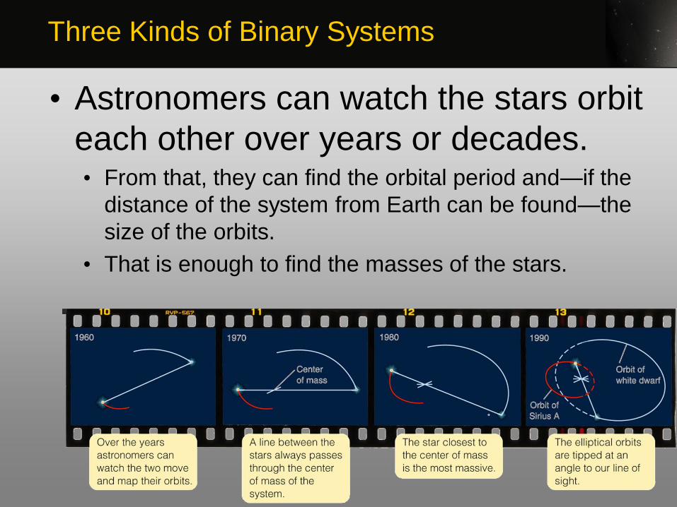
• Astronomers can watch the stars orbit

each other over years or decades.• From that, they can find the orbital period and—if the

distance of the system from Earth can be found—the

size of the orbits.

• That is enough to find the masses of the stars.


• Many visual binaries have such

large orbits their orbital periods are

hundreds or thousands of years.• Astronomers have not yet seen them complete

an entire orbit.


• Also, many binary stars orbit so

close to each other they are not

visible as separate stars.• Such systems can’t be analyzed as a visual

binary.


• If the stars in a binary system are close

together, a telescope view—limited by

diffraction and by the atmospheric

blurring called seeing—shows a single

point of light.


• Only by looking at a spectrum—which is

formed by light from both stars and contains

spectral lines from both—can astronomers

tell that there are two stars present and not

one.

• Such a system is a spectroscopic binary system.


• Familiar examples of spectroscopic

binary systems are

the stars Mizar and

Alcor in the handle

of the Big Dipper.


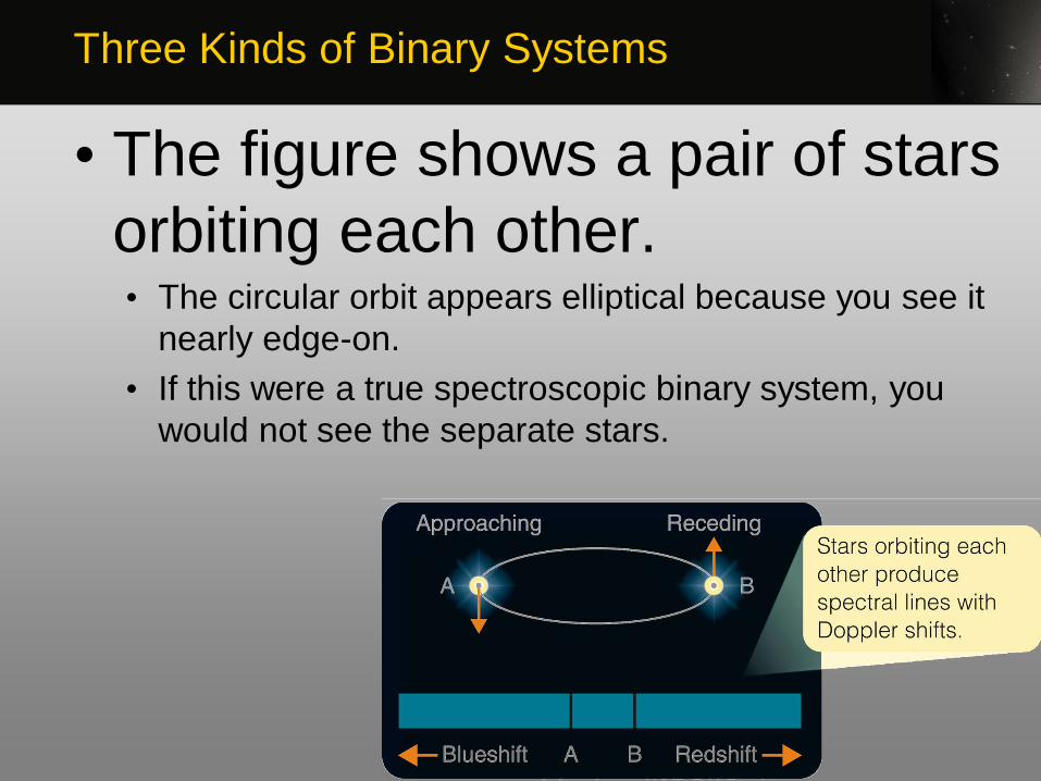
• The figure shows a pair of stars

orbiting each other.• The circular orbit appears elliptical because you see it

nearly edge-on.

• If this were a true spectroscopic binary system, you

would not see the separate stars.


• Nevertheless, the

Doppler shift would show

you there were two stars

orbiting each other.


• As the two stars move in

their orbits, they alternately

approach toward and

recede from Earth.


• Their spectral lines are

Doppler shifted alternately

toward blue and then red

wavelengths.


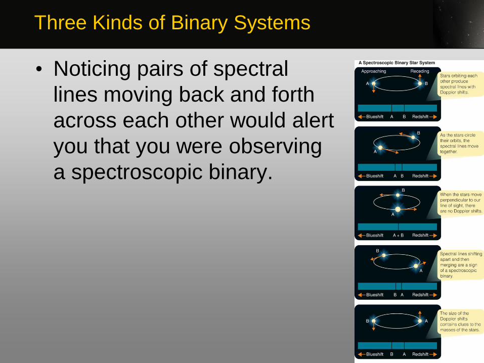
• Noticing pairs of spectral

lines moving back and forth

across each other would alert

you that you were observing

a spectroscopic binary.


• Although spectroscopic binaries are

very common, they are not as useful

as visual binaries.• Astronomers can find the orbital period easily—but

they can’t find the true size of the orbits, because

there is no way to find the angle at which the orbits

are tipped.

• That means they can’t find the true masses of a

spectroscopic binary.

• All they can find is a lower limit to the masses.


• If the plane of the orbits is nearly edge-on

to Earth, then the stars can cross in front

of each other as seen from Earth.

• When one star moves in front of the other,

it blocks some of the light, and the star is

eclipsed.

• Such a system is called an eclipsing binary

system.


• Seen from Earth, the two stars are not

visible separately.

• The system looks like a single point of light.

• However, when one star moves in front of

the other star, part of the light is blocked,

and the total brightness of the point of light

decreases.


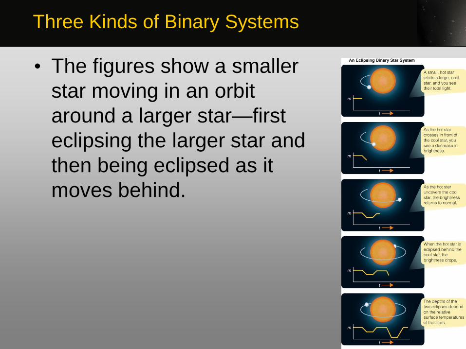
• The figures show a smaller

star moving in an orbit

around a larger star—first

eclipsing the larger star and

then being eclipsed as it

moves behind.


• The resulting variation

in the brightness of the

system is shown as a

graph of brightness

versus time—a light

curve.


• The light curves of eclipsing

binary systems contain

plenty of information about

the stars.

• However, they can be

difficult to analyze.• The figures show an idealized

example of such a system.


• Once the light curve of an eclipsing

binary system has been accurately

observed, astronomers can construct

a chain of inference that leads to the

masses of the stars.


• They can find the orbital period easily and

can get spectra showing the Doppler shifts

of the two stars.

• They can find the orbital speed because

they don’t have to correct for the

inclination of the orbits.• You know the orbits are nearly edge-on, or there

would not be eclipses.

• From that, astronomers can find the size of the orbits

and the masses of the stars.


• Earlier in the chapter, luminosity and

temperature were used to calculate the radii

of stars.

• However, eclipsing binary systems give a

way to check those calculations—by

measuring the sizes of a few stars directly. • The light curve shows how long it takes for the stars to

cross in front of each other.

• Multiplying these time intervals by the orbital speeds

gives the diameters of the stars.


• There are complications due to the

inclination and eccentricity of orbits.

• Often, though, these effects can be

taken into account.• So, observations of an eclipsing binary system can

directly give you not only the masses of its stars but

also their diameters.


• From the study of binary stars,

astronomers have found that the masses

of stars range from roughly 0.1 solar

masses to nearly 100 solar masses.• The most massive stars ever found in a binary

system have masses of 83 and 82 solar masses.


• A few other stars are believed to be

more massive—100 solar masses to

150 solar masses.• However, they do not lie in binary systems.

• So, astronomers must estimate their masses.


• You have achieved the five

goals set at the start of the

chapter.• You know how to find the distances, luminosities,

temperatures, diameters, and masses of stars.

Typical Stars

• Now, you can put those data

together to paint a family portrait

of the stars.• As in human family portraits, both similarities and

differences are important clues to the history of the

family.

Typical Stars

• The H-R diagram is filled with patterns

that give you clues as to how stars are

born, how they age, and how they die.• When you add your data, you see traces of those

patterns.

Luminosity, Mass, and Density

• If you label an H-R

diagram with the

masses of the stars

determined by

observations of

binary star systems,

you will discover

that the main-

sequence stars

are ordered by

mass.


• The most massive main-sequence stars are the hot stars.

• Going down the main sequence, you will find lower-mass stars.

• The lowest-mass stars are the coolest, faintest main-sequence stars.


• Stars that do not lie on

the main sequence are

not in order according

to mass. • Some giants and

supergiants are

massive, whereas

others are no more

massive than the sun.

• All white dwarfs have

about the same mass

—usually in the narrow

range of 0.5 to about

1.0 solar masses.


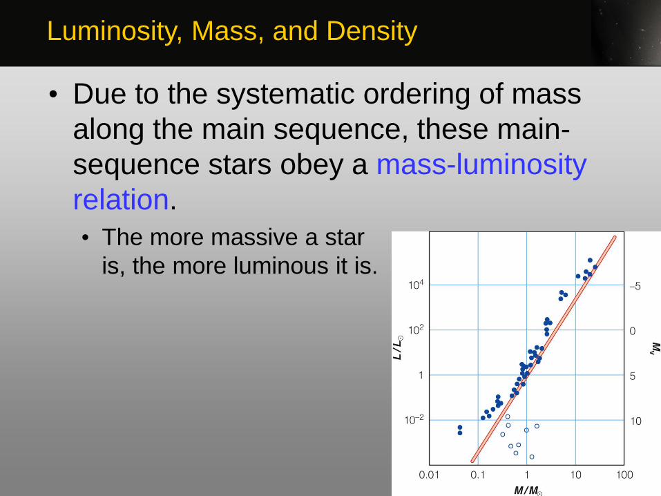
• Due to the systematic ordering of mass

along the main sequence, these main-

sequence stars obey a mass-luminosity

relation.

• The more massive a star

is, the more luminous it is.


• In fact, the mass-luminosity relation can

be expressed as follows.

• Luminosity is proportional to mass to

the 3.5 power.• For example, a star with a mass of 4.0 MΘ can be

expected to have a luminosity of about 43.5 or 128 LΘ.


• Giants and supergiants do not follow

the mass-luminosity relation very

closely.

• White dwarfs do not follow it at all.


• Though mass alone does not reveal

any pattern among giants, supergiants,

and white dwarfs, density does.• Once you know a star’s mass and diameter, you can

calculate its average density by dividing its mass by its

volume.


• Stars are not uniform in density.

• They are most dense at their centers

and least dense near their surface.• The center of the sun is about 100 times as dense as

water.

• In contrast, its density near the photosphere is about

3,400 times less dense than Earth’s atmosphere at

sea level.


• A star’s average density is

intermediate between its central and

surface densities.• The sun’s average density is approximately 1 g/cm3—

about the density of water.

• Main-sequence stars have average densities similar to

the sun’s density.


• As you learned earlier in the discussion

about luminosity classification, giant stars

are much larger in diameter than the main-

sequence stars but not much larger in mass.

• So, giants have low average densities—

ranging from 0.1 to 0.01 g/cm3.


• The enormous supergiants have still

lower densities—ranging from 0.001

to 0.000001 g/cm3.• These densities are thinner than the air we breathe.

• If you could insulate yourself from the heat, you

could fly an airplane through these stars.

• Only near the center would you be in any danger—

we can calculate that the material there is very

dense.


• The white dwarfs have masses about

equal to the sun’s, but are very small—

only about the size of Earth.• Thus, the matter is compressed to densities of

3,000,000 g/cm3 or more.

• On Earth, a teaspoonful of this material would weigh

about 15 tons.


• Density divides stars into three

groups.• Most stars are main-sequence stars with densities

similar to the sun’s.

• Giants and supergiants are very-low density stars.

• White dwarfs are high-density stars.


• If you want to know what the average

person thinks about a certain subject, you

take a survey.

• If you want to know what the average star

is like, you can survey the stars.• Such surveys reveal important relationships among

the family of stars.

Surveying the Stars

• Over the years, many astronomers have

added their results to the growing collection

of data on star distances, luminosities,

temperatures, sizes, and masses.

• They can now analyze those data to search

for relationships between these and other

parameters.• As the 21st century begins, astronomers are deeply

involved in massive surveys.

Surveying the Stars

• Powerful computers to control

instruments and analyze data make

such immense surveys possible.• For example, the Sloan Digital Sky Survey will

eventually map a quarter of the sky—measuring the

position and brightness of 100 million stars and

galaxies.

• Also, the Two Micron All Sky Survey (2MASS) has

mapped the entire sky at three near-infrared

wavelengths.

Surveying the Stars

• A number of other sky surveys

are underway.• Astronomers will ‘mine’ these mountains of data

for decades to come.

Surveying the Stars

• What could you learn about

stars from a survey of the stars

near the sun? • The evidence astronomers have is that the sun is in a

typical place in the universe.

• Therefore, such a survey could reveal general

characteristics of the stars.

Surveying the Stars

• There are three important

points to note about the family

of stars.

Surveying the Stars

• One, taking a survey is difficult

because you must be sure to get an

honest sample.• If you don’t survey enough stars, your results can be

biased.

Surveying the Stars

• Two, M dwarfs and white dwarfs are

so faint that they are difficult to find

even near Earth.

• They may be undercounted in surveys.

Surveying the Stars

• Finally, luminous stars—although they

are rare—are easily visible even at

great distances.• Typical nearby stars

have lower luminosity

than our sun.

Surveying the Stars

• The night sky is a beautiful carpet of

stars.

• Some are giants and supergiants, and

some are dwarfs.• The family of stars is rich in its diversity.

Surveying the Stars

• Pretend space is like a very clear

ocean in which you are

swimming.• When you look at the night sky, you are seeing

mostly ‘whales’—the rare very large and luminous

stars, mostly far away.

• If instead you cast a net near your location, you

would mostly catch ‘sardines’—very-low-luminosity

M dwarfs that make up most of the stellar population

of the universe.

Surveying the Stars

• This chapter set out to find the basic

properties of stars.

• Once you found the distance to the stars,

you were able to find their luminosities.

• Knowing their luminosities and

temperatures gives you their diameters.

• Studying binary stars gives you their

masses. • These are all rather mundane data.

Surveying the Stars

• However, you have now

discovered a puzzling situation.• The largest and most luminous stars are so rare you

might joke that they hardly exist.

• The average stars are such small low-mass things they

are hard to see even if they are near Earth in space.

Surveying the Stars

• Why does nature make stars

in this peculiar way?• To answer that question, you must explore the

birth, life, and death of stars.

Surveying the Stars

The Scale of the Cosmos - Los Angeles Mission College

Documents

Transcript of The Scale of the Cosmos - Los Angeles Mission College