THE ROLE OF PARASITES, DISEASES, MINERAL LEVELS, AND LOW FAWN

SURVIVAL IN A DECLINING PRONGHORN POPULATION IN THE

TRANS-PECOS REGION OF TEXAS

A Thesis

By

James H. Weaver

Submitted to the College of Agricultural and Natural Resource Sciences

Sul Ross State University

in partial fulfillment of the requirements for the degree of

MASTER OF SCIENCE

December 2013

Major Subject: Range and Wildlife Management

THE ROLE OF PARASITES, DISEASES, MINERAL LEVELS, AND LOW FAWN

SURVIVAL IN A DECLINING PRONGHORN POPULATION IN THE

TRANS-PECOS REGION OF TEXAS

A Thesis

By

James H. Weaver

Approved as to style and content by:

_______________________________ _______________________________

Louis A. Harveson, Ph.D. Kenneth A. Waldrup, Ph.D.

(Committee Chair) (Member)

_______________________________ _______________________________

Patricia M. Harveson, Ph.D. Shawn S. Gray, M.S.

(Member) (TPWD Representative)

_______________________________

Robert J. Kinucan, Ph.D.

(Dean of Agricultural and Natural Resource Sciences)

iii

ABSTRACT

Since the late 1980s, pronghorn populations of west Texas have been in a steady

decline. Texas Parks and Wildlife Department’s (TPWD) 2012 surveys showed that the

population was estimated at 2,751 animals, a 75-year low for the region. In 2009, a study

was initiated to determine some of the leading causes for the recent decline in this region,

including prevalence of diseases, mineral concentrations, parasites, and fawn survival. I

found an average prevalence of titers for blue tongue virus (BTV) to be 97% and 92% for

epizootic hemorrhagic disease (EHD) in 2010 and 2011, respectively. Because trace

mineral levels (e.g., copper and selenium) have also been tied to productivity in

pronghorn, I compared mineral levels between the Trans-Pecos and Panhandle. Copper

serum levels were the same between regions (P = 0.199), but copper liver levels (P =

0.002), and selenium levels were different (P < 0.001). I also investigated the roles of

parasites and predation as a limiting factor for pronghorn production in the Trans-Pecos. I

found a difference when comparing Haemonchus worm counts (P = 0.041) and fecal egg

counts (P < 0.001) between regions (Trans-Pecos, Panhandle). In 2011, surveys showed

some areas to have fawn crops as low as 0% (0 fawns: 100 does), with a Trans-Pecos

average at 10%. In 2012, TPWD surveys indicated that the fawn crops averaged about

16% Trans-Pecos wide. I conducted a pronghorn fawn survival study to determine major

causes of mortality. Predation was the major cause of mortality in both 2011 and 2012.

Bobcat (Lynx rufus) predation accounted for 32%, unknown predation accounted for

28%, and coyote (Canis latrans) predation accounted for 24% of all mortalities. Marginal

mineral levels, high Haemonchus loads, and high predation on pronghorn fawns appear to

be having a negative impact on pronghorn populations in the Trans-Pecos.

iv

DEDICATION

To my wife, Kayla Weaver, son, Jaxon Weaver, and parents, Ernie and Vicki Weaver

for your amazing love, sacrifice, and support, that allowed me to follow my dreams.

v

ACKNOWLEDGEMENTS

I would like to first give thanks to the landowners that opened their homes, lives,

and ranches to me for this project: Bill and Jill Miller, Albert Miller, Stewart Sasser,

Robert Potts, Evan Roderick, Clay Evans, Rob Beard, and the Hagner family.

Financial support for this project was primarily provided by Texas Parks and

Wildlife Department (TPWD). I would like to thank TPWD staff Shawn Gray, Billy

Tarrant, Michael Sullins, Michael Janis, Johnny Arredondo, and Misty Sumner for their

assistance and support throughout the study.

Partial financial support for this project was provided by West Texas Chapter of

Safari Club International. The help and support of this organization has been tremendous.

I am very thankful for my committee chair Dr. Louis A. Harveson, which gave

me the opportunity to conduct research under his advice and who has always found the

time to help me through problems, both academic and personal. I would also like to thank

committee members Dr. Kenneth Waldrup, Dr. Patricia Moody Harveson, and Shawn

Gray for their continued support throughout the study.

I am grateful for the opportunity to have been a part of the Trans-Pecos Pronghorn

Working Group, which is made up of some of the best people I know. They have always

put pronghorn first and have been great mentors to me both professionally and with my

personal life.

vi

I would also like to thank Dr. Dan E. McBride for helping me get access to

property, collecting samples, and for sharing his dedication, love, knowledge, and passion

for pronghorn with me.

I could not have done this project without the help of my friends, fellow graduate

students, and technicians: Justin Hoffman, Lalo Gonzalez, Andy James, Thomas Janke,

Joshua Cross, Daniel Tidwell, Jon Falcone, Chelsea Cadman, and the many volunteers.

Finally, I would like to thank my wife, Kayla, who has always supported and

loved me no matter what, and has always sacrificed so that I can chase my dreams.

vii

TABLE OF CONTENTS

Page

ABSTRACT……………………………………………………………….

……………………………………

iii

DEDICATION……………………………………………………………. iv

ACKNOWLEDGEMENTS……………………………………………….

……………………………………

v

TABLE OF CONTENTS………………………………………………….

……………………………………

vii

LIST OF TABLES...………...……………………………………………. viii

LIST OF FIGURES……………………………………………………….

ix

LIST OF APPENDICES………………………………………………….. xi

CHAPTER I: INTRODUCTION……………………………….………...

1

CHAPTER II: MINERAL LEVELS AND DISEASE PREVALENCE IN

TEXAS PRONGHORN…….…………………………………………….

8

CHAPTER III: HAEMONCHUS-PRONGHORN INTERACTIONS IN

TEXAS…………………………………………………………………….

32

CHAPTER IV: FAWN SURVIVAL OF PRONGHORN IN THE

TRANS-PECOS…..…….………………………………………………....

57

APPENDICES……………………………………………………………. 89

VITA...…………………………………………………………………….

.

96

viii

LIST OF TABLES

Table Page

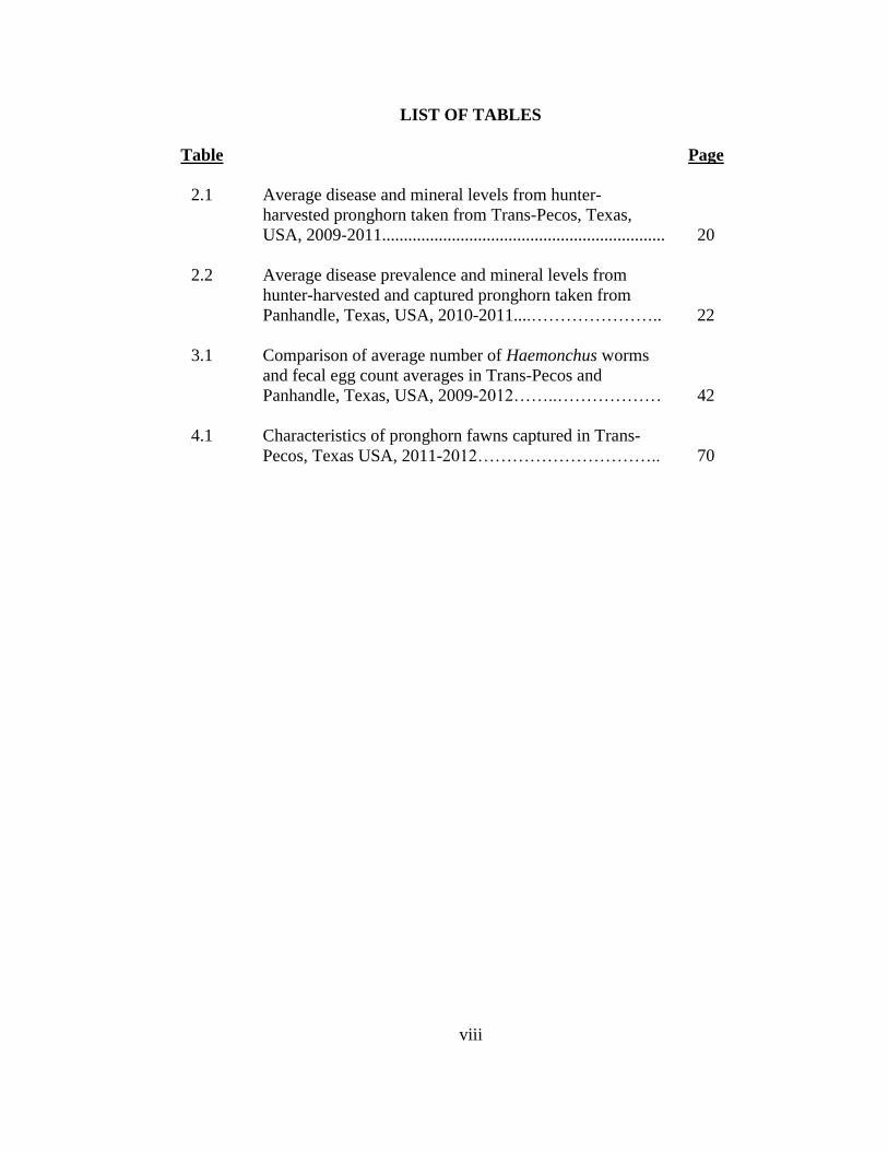
2.1 Average disease and mineral levels from hunter-

harvested pronghorn taken from Trans-Pecos, Texas,

USA, 2009-2011.................................................................

20

2.2 Average disease prevalence and mineral levels from

hunter-harvested and captured pronghorn taken from

Panhandle, Texas, USA, 2010-2011....…………………..

22

3.1 Comparison of average number of Haemonchus worms

and fecal egg count averages in Trans-Pecos and

Panhandle, Texas, USA, 2009-2012……..………………

42

4.1 Characteristics of pronghorn fawns captured in Trans-

Pecos, Texas USA, 2011-2012…………………………..

70

ix

LIST OF FIGURES

Figure Page

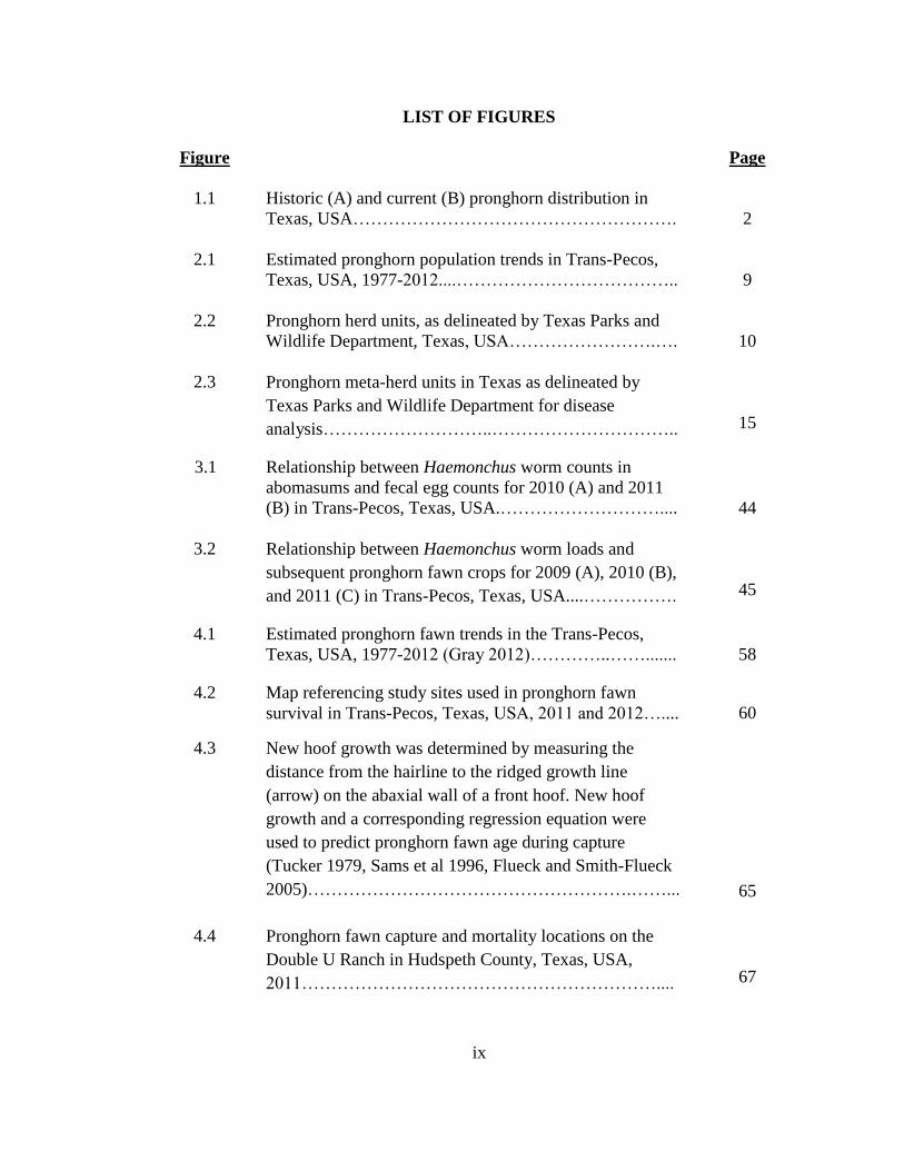
1.1

Historic (A) and current (B) pronghorn distribution in

Texas, USA……………………………………………….

2

2.1 Estimated pronghorn population trends in Trans-Pecos,

Texas, USA, 1977-2012....………………………………..

9

2.2 Pronghorn herd units, as delineated by Texas Parks and

Wildlife Department, Texas, USA…………………….….

10

2.3 Pronghorn meta-herd units in Texas as delineated by

Texas Parks and Wildlife Department for disease

analysis………………………..…………………………..

15

3.1 Relationship between Haemonchus worm counts in

abomasums and fecal egg counts for 2010 (A) and 2011

(B) in Trans-Pecos, Texas, USA.………………………....

44

3.2 Relationship between Haemonchus worm loads and

subsequent pronghorn fawn crops for 2009 (A), 2010 (B),

and 2011 (C) in Trans-Pecos, Texas, USA....…………….

45

4.1 Estimated pronghorn fawn trends in the Trans-Pecos,

Texas, USA, 1977-2012 (Gray 2012)…………..…….......

58

4.2 Map referencing study sites used in pronghorn fawn

survival in Trans-Pecos, Texas, USA, 2011 and 2012…....

60

4.3 New hoof growth was determined by measuring the

distance from the hairline to the ridged growth line

(arrow) on the abaxial wall of a front hoof. New hoof

growth and a corresponding regression equation were

used to predict pronghorn fawn age during capture

(Tucker 1979, Sams et al 1996, Flueck and Smith-Flueck

2005)……………………………………………….……...

65

4.4 Pronghorn fawn capture and mortality locations on the

Double U Ranch in Hudspeth County, Texas, USA,

2011……………………………………………………....

67

x

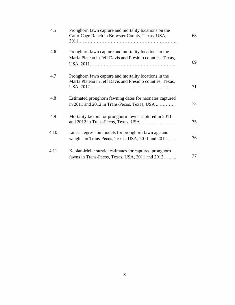
4.5 Pronghorn fawn capture and mortality locations on the

Catto-Cage Ranch in Brewster County, Texas, USA,

2011……………………………………………………….

68

4.6 Pronghorn fawn capture and mortality locations in the

Marfa Plateau in Jeff Davis and Presidio counties, Texas,

USA, 2011………………………………………………..

69

4.7 Pronghorn fawn capture and mortality locations in the

Marfa Plateau in Jeff Davis and Presidio counties, Texas,

USA, 2012………………………………………………..

71

4.8 Estimated pronghorn fawning dates for neonates captured

in 2011 and 2012 in Trans-Pecos, Texas, USA ...………..

73

4.9 Mortality factors for pronghorn fawns captured in 2011

and 2012 in Trans-Pecos, Texas, USA…………………...

75

4.10 Linear regression models for pronghorn fawn age and

weights in Trans-Pecos, Texas, USA, 2011 and 2012……

76

4.11 Kaplan-Meier survial estimates for captured pronghorn

fawns in Trans-Pecos, Texas, USA, 2011 and 2012……...

77

xi

LIST OF APPENDICES

Appendices Page

A. Horn measurements, cementum annuli age estimations,

and kidney fat indices collected from harvested

pronghorn bucks in Trans-Pecos, Texas, 2010-2011........

89

1

CHAPTER I: INTRODUCTION

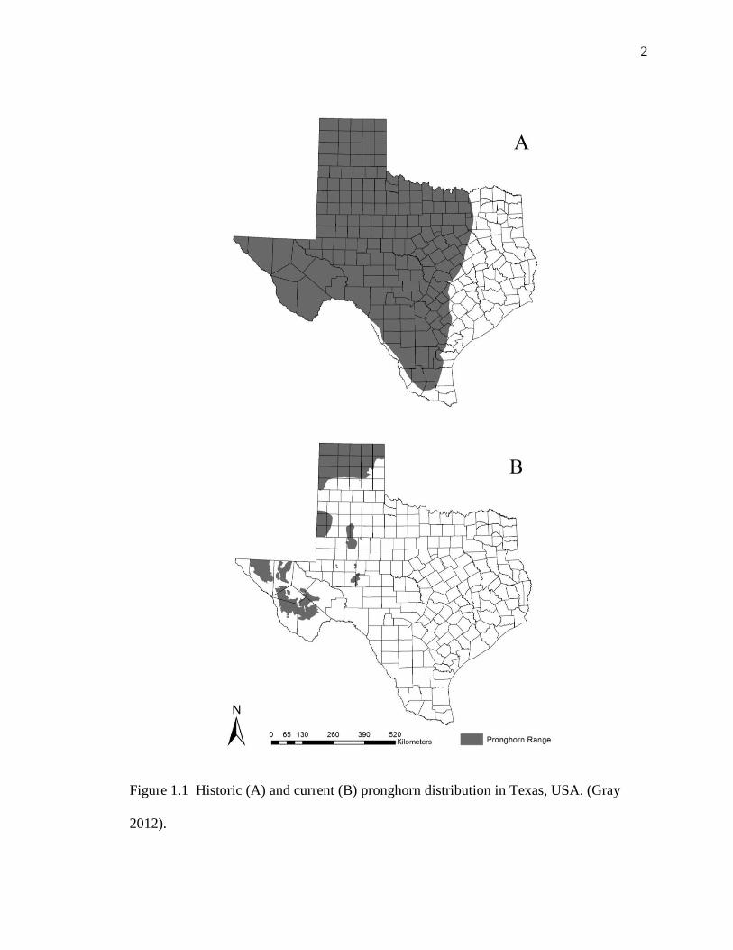
Historic distribution of pronghorn (Antilocapra americana) in Texas included most areas

west of the 97th

meridian (Figure 1.1A) which accounted for approximately two-thirds of

the state (Buechner 1950). Presently, pronghorn are now limited to the Panhandle, Trans-

Pecos, and portions of the Rolling Plains ecoregions (Figure 1.1B) (Gray 2012).

Pronghorn populations have not only been reduced in distribution but also in population

size. Aerial surveys conducted by Texas Parks and Wildlife Department in the Trans-

Pecos in the summer of 2012, revealed populations numbers had reached an 75-year low

with an estimated 2,751 pronghorn (Gray 2012). As recently as 1987, pronghorn

populations were estimated to be 17,226 animals in the Trans-Pecos. Precipitation has

been tied to productivity in pronghorn for this region, and can explain most of the

changes in pronghorn population trends (Simpson et al. 2006). In 2009 and 2010, the

Trans-Pecos had favorable conditions due to well-timed precipitation, but populations

continued to plummet. Since precipitation was not seen to be the issue regarding the

pronghorn decline, research was conducted to determine the role other factors were

having on pronghorn populations. Diseases, mineral levels, parasites, and pronghorn

fawn survival were deemed to be possible reasons for the decline.

Diseases such as blue tongue virus (BTV) and Epizootic Hemorrhagic Disease

(EHD) have been known to cause large die-offs in other western states (Thorne et al.

1988). Pronghorn populations sampled in Arizona showed that 78.5% of pronghorn

____________

This thesis follows the style of the Journal of Wildlife Management

2

Figure 1.1 Historic (A) and current (B) pronghorn distribution in Texas, USA. (Gray

2012).

3

tested had been exposed to hemorrhagic disease (Heffelfinger and Olding 1996,

Heffelfinger et al. 1999). This is evidence that pronghorn populations in Arizona and

possibly other southern populations have a higher tolerance to hemorrhagic disease,

which decreases the chance of high mortality rates (O’Gara 2004c).

There is also little known about effects of trace minerals in pronghorn and what

problems are caused by deficiencies. Pronghorn populations with higher concentrations

of copper and selenium have been shown to have higher production (O’Gara 2004a).

Dunbar et al. (1999) reported marginal levels for copper and selenium in both adults and

fawns in a declining pronghorn population in Oregon. Zimmerman et al. (2008) found

that copper influenced the production of some free-ranging ruminants. Puls (1994) and

Miller et al. (2001) reported copper deficiencies to cause enzootic ataxia, weight loss,

infertility, anemia, diarrhea, depressed growth, heart failure, skeletal defects and

increased susceptibility to infectious diseases. White muscle disease is one of the major

effects of selenium deficiencies, which can lead to death (Flueck and Smith-Flueck

1990). Since pronghorn do not do well in captivity, normal levels of trace minerals are

still unclear at this time and most comparisons are done between domestic animals

(Dunbar et al. 1999).

Haemonchus was found in pronghorn from the Trans-Pecos region in the late

1960s but this was not seen to be significant (Hailey 1968). Hailey (1968) concluded the

dry climate of the Trans-Pecos helped limit the spread of parasites and diseases and were

not thought to be of concern. Haemonchus is a very productive parasite that can have

lethal effects on both domestic and wild ruminants, and can affect animals, populations,

4

and the industries depending on these animals (McGhee et al. 1981, Newton and Munn

1999). Adult Haemonchus worms ingest blood from wounds in the abomasum and lay

eggs, which are then carried out of the host by defecation (Zajac 2006). Haemonchus can

cause many problems to a host including, weakness, weight loss, anemia, and in many

cases death (McGhee et al. 1981, Simpson 2000, Zajac 2006).

Fawn survival is critical for populations to thrive (Sievers 2004). Texas Parks and

Wildlife Department has documented low fawn crops throughout the Trans-Pecos over

the last several years (Gray 2012). Predation is usually the primary cause of pronghorn

fawn mortality, which can have a greater impact in small populations (Beale and Smith

1973). Where there is a high nutritional plane, pronghorn populations can be very

productive and breeding can begin as early as fawns (O’Gara 2004b). Fawn survival may

be limiting population recovery for declining Trans-Pecos populations.

The recent decline of pronghorn in the Trans-Pecos is alarming and is not

completely understood. In the Texas Panhandle, pronghorn populations are thriving and

are used for comparison throughout this thesis. To better understand the recent decline

and why these populations are continuing to struggle, I initiated a study in October 2009

to collect disease, parasite, and fawn mortality data on pronghorn populations in the

Trans-Pecos. Specifically, I report on mineral levels and disease prevalence in Texas

pronghorn (Chapter 2), Haemonchus-pronghorn interactions in Texas (Chapter 3), and

fawn survival of pronghorn in the Trans-Pecos (Chapter 4).

5

LITERATURE CITED

Beale, D. M., and A. D. Smith. 1973. Mortality of pronghorn antelope fawns in western

Utah. Journal of Wildlife Management 37:343–352.

Buechner, H. K. 1950. Life history, ecology, and range use of the pronghorn

antelope in Trans‐Pecos of Texas. American Midland Naturalist 43:257–354.

Dunbar, M. R., R. Velarde, M. A. Gregg, and M. Bray. 1999. Health evaluation of a

pronghorn antelope population in Oregon. Journal of Wildlife Diseases 35:496-

510.

Flueck, W. T., and J. M. Smith-Flueck. 1990. Selenium deficiency in deer: The effect of

a declining selenium cycle? Transactions of the Congress of the International

Union of Game Biologists 19:292-301.

Gray, S. S. 2012. Big game research and surveys: Pronghorn harvest recommendations.

Federal Aid Project W-127-R-20. Texas Parks and Wildlife Department, Austin,

Texas, USA.

Hailey, T. L. 1968. A handbook for pronghorn antelope management in Texas. Federal

aid report series number 20, Texas Parks and Wildlife Department, Austin, Texas,

USA.

Heffelfinger, J. R., and R. J. Olding. 1996. Occurrence and distribution of blue tongue in

pronghorn antelope. P-R Performance Report, Project W-53-M-47. Arizona

Department of Game and Fish, Phoenix, Arizona, USA.

6

Heffelfinger, J. R., R. J. Olding, T. H. Noon, M. R. Shupe, and D. P. Betzer. 1999.

Copper/selenium levels and occurrence of bluetongue virus in Arizona pronghorn.

Proceedings of the Pronghorn Antelope Workshop 18:32–42.

McGhee, M. B., V. F. Nettles, E. A. Rollor, III, A. K. Prestwood, and W. R. Davidson.

1981. Studies on cross‐transmission and pathogenicity of Haemonchus contortus

in white‐tailed deer, domestic cattle and sheep. Journal of Wildlife Diseases

17:353–364.

Miller, M., S. Amsel, J. Boehm, and B. Gonzales. 2001. Presumptive copper deficiency

in hand-reared captive pronghorn (Antilocapra americana) fawns. Journal of Zoo

and Wildlife Medicine 32:373-378.

Newton, S. E., and E. A. Munn. 1999. The development of vaccines against

gastrointestinal nematode parasites, particularly Haemonchus contortus.

Parasitology Today 15:116–122.

O’Gara, B. W. 2004a. Physiology and genetics. Pages 230-274 in B. W. O’ Gara, and J.

D. Yoakum, editors. Pronghorn: Ecology and management. University Press of

Colorado, Boulder, Colorado, USA.

O’Gara, B. W. 2004b. Reproduction. Pages 275-298 in B. W. O’ Gara, and J. D.

Yoakum, editors. Pronghorn: Ecology and management. University Press of

Colorado, Boulder, Colorado, USA.

O’Gara, B. W. 2004c. Diseases and parasites. Pages 299-336 in B. W. O’ Gara, and J. D.

Yoakum, editors. Pronghorn: Ecology and management. University Press of

Colorado, Boulder, Colorado, USA.

7

Puls, R. 1994. Mineral levels in animal health diagnostic data, second edition. Sherpa

International, Clearbrook, British Columbia, Canada.

Sievers, J. D. 2004. Factors influencing a declining pronghorn population in Wind Cave

National Park, South Dakota. Thesis, South Dakota State University, Brookings,

USA.

Simpson, D. C., L. A. Harveson, C. E. Brewer, R. E. Walser, and A. R. Sides. 2006.

Influence of precipitation on pronghorn demography in Texas. Journal of Wildlife

Management 71:906-910.

Simpson, H. V. 2000. Pathophysiology of abomasal parasitism: Is the host or parasite

responsible? Veterinary Journal 160:177–191.

Thorne, E. T., E. S. Williams, T. R. Spraker, W. Helms, and T. Segerstrom. 1988.

Bluetongue in free‐ranging pronghorn antelope (Antilocapra americana) in

Wyoming: 1976 and 1984. Journal of Wildlife Diseases 24:113–119.

Zajac, A. M. 2006. Gastrointestinal nematodes of small ruminants: Life cycle,

anthelmintics, and diagnosis. Veterinary Clinics‐Food Animal Practice 22:529–

541.

Zimmermann, T. J., J. A. Jenks, D. M. Leslie, Jr., and R. D. Neiger. 2008. Hepatic

minerals of white‐tailed and mule deer in the southern Black Hills, South Dakota.

Journal of Wildlife Diseases 44:341–350.

8

CHAPTER II: MINERAL LEVELS AND DISEASE PREVALENCE IN TEXAS

PRONGHORN

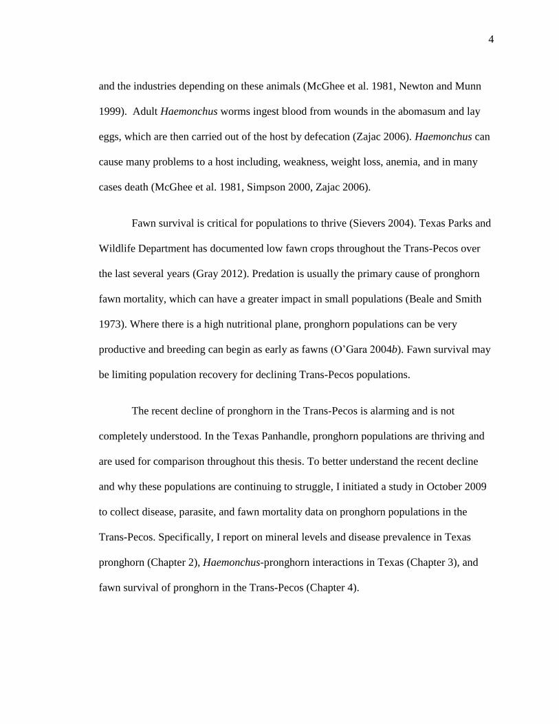
Since the late 1980s pronghorn (Antilocapra americana) populations in the Trans-Pecos

region of Texas have been on a steady decline (Gray 2012). In 2012, Texas Parks and

Wildlife Department (TPWD) surveys documented a new 75-year low, with the

population estimated to be 2,751 animals (Figure 2.1; Gray 2012). To monitor

populations, TPWD surveys herd units that have been delineated by the department

(Figure 2.2).

In states such as Wyoming, bluetongue virus (BTV) and epizootic hemorrhagic

disease (EHD) can cause large die-offs and have a large impact on pronghorn populations

(Thorne et al. 1988). In 1976, ≥ 3,200 pronghorn died during a bluetongue epizootic in

eastern Wyoming (Thorne et al. 1988). Thorne et al. (1988) reported another BTV

epizootic in northeastern Wyoming in 1984 where 300 pronghorn were known to die.

Two captive pronghorn in Oregon also died due to EHD and/or BTV (Kistner et al.

1975). Samples tested in Arizona showed 78.5% of pronghorn tested positive for

exposure to hemorrhagic disease (Heffelfinger and Olding 1997, Heffelfinger et al.

1999). This indicates that Arizona and possibly other southern populations can be

exposed to hemorrhagic disease without experiencing high mortality rates (O’Gara 2004).

Positive titers for BTV and EHD have been reported for a variety of ungulates in

west Texas. Pittman (1987) reported prevalence of BTV for mule deer (Odocoileus

hemionus) at Black Gap WMA at 76.7%. On Sierra Diablo WMA, Waldrup et al. (1989)

9

Figure 2.1 Estimated pronghorn population trends in Trans-Pecos, Texas, USA 1977-

2012 (Gray 2012).

10

Figure 2.2 Pronghorn herd units, as delineated by Texas Parks and Wildlife Department,

Texas, USA (Gray 2012).

11

reported prevalence of BTV and EHD in mule deer at 25% and 20%, respectively.

Prevalence of BT and EHD antibodies for aoudad (Ammotragus lervia) on Big Bend

Ranch State Park was at 56% and 33%, respectively (TPWD unpublished data). The

prevalence of BTV and EHD in pronghorn in the Trans-Pecos region of Texas is

unknown, however, in Arizona Heffelfinger and Olding (1997) found 78.5% of 288

hunter-harvested pronghorn tested positive for exposure to BTV.

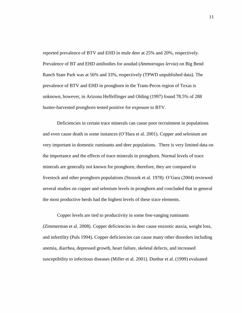
Deficiencies in certain trace minerals can cause poor recruitment in populations

and even cause death in some instances (O’Hara et al. 2001). Copper and selenium are

very important in domestic ruminants and deer populations. There is very limited data on

the importance and the effects of trace minerals in pronghorn. Normal levels of trace

minerals are generally not known for pronghorn; therefore, they are compared to

livestock and other pronghorn populations (Stoszek et al. 1978). O’Gara (2004) reviewed

several studies on copper and selenium levels in pronghorn and concluded that in general

the most productive herds had the highest levels of these trace elements.

Copper levels are tied to productivity in some free‐ranging ruminants

(Zimmerman et al. 2008). Copper deficiencies in deer cause enzootic ataxia, weight loss,

and infertility (Puls 1994). Copper deficiencies can cause many other disorders including

anemia, diarrhea, depressed growth, heart failure, skeletal defects, and increased

susceptibility to infectious diseases (Miller et al. 2001). Dunbar et al. (1999) evaluated

12

the health of a declining pronghorn population in Oregon and concluded that both copper

and selenium levels were marginal.

Selenium levels have also been tied to infertility in small ruminants. Selenium

deficiency in domestic ruminants is largely associated with muscular degeneration,

reproductive problems, and illthrift (Flueck and Smith-Flueck 1990). White muscle

disease is most common and can cause death, especially in young (Flueck and Smith-

Flueck 1990). A selenium deficiency was suspected by Starkley et al. (1982) to be

involved in lowered reproductive performance of Roosevelt elk (Cervus elaphus

roosevelti). Roosevelt elk are found on the coastal Pacific Northwest, which is an area

known to be deficient in selenium where domestic livestock require selenium

supplementation (Starkley et al. 1982). Selenium deficiency causes lowered fertility of

adults and high mortality of young (Church and Pond 1978).

There are many known factors that affect pronghorn populations and other wild

ungulates. I initiated a study to determine the prevalence of BTV and EHD, and to

document the levels of selenium and copper in pronghorn from the Trans-Pecos region. I

predicted (1) that pronghorn in the Trans-Pecos would have a high prevalence of BTV

and EHD titers, and (2) would exhibit marginal levels of the trace minerals copper and

selenium.

STUDY AREA

The study area consisted of 7 sampling units in the Trans-Pecos region, 1 sampling unit

13

in the western Edwards Plateau Ecoregion, and also sampling 2 units in the northwest and

northeast Texas Panhandle.

Trans-Pecos

The Trans-Pecos is a highly diverse landscape, which contains a wide variety of habitat

types and natural resources. The Trans‐Pecos region is approximately 7.3 million ha and

is located in the Chihuahuan Desert Biotic Province. The Trans‐Pecos is made up of 9

counties that are bordered by the Rio Grande, New Mexico, and the Pecos River (Hatch

et al. 1990). Elevation ranges from 762 in the low grasslands to 2,667 in the scattered

desert islands. Basins usually receive 20-30 cm of annual precipitation, whereas the

higher elevations receive 30-46 cm. Soils vary throughout the region with rocky soils on

mountains and hills, gravelly soils in the lowlands, and sandy soils in the flats and desert

washes (Harveson 2006). Pronghorn habitat is generally described as low-rolling, wide

open, expansive grasslands or shrub steppes (O’Gara and Yoakum 1992). Within the

Trans‐Pecos, pronghorn are directly associated with the Desert Grassland Biotic District

(Buechner 1950).

Vegetation types common in the study area included yucca (Yucca spp.)

savannahs, grama (Bouteloua spp.) grasslands, creosote (Larrea tridentata) shrublands

(Canon and Bryant 1997) and tobosa (Pleuraphis mutica) grasslands. Land use practices

vary across the region, but most rangelands are used for agricultural purposes (livestock

grazing or wildlife enterprises; Harveson 2006). The 7 sampling units pronghorn samples

were taken from in the Trans-Pecos consisted of Culberson, Hudspeth, Marathon, Marfa

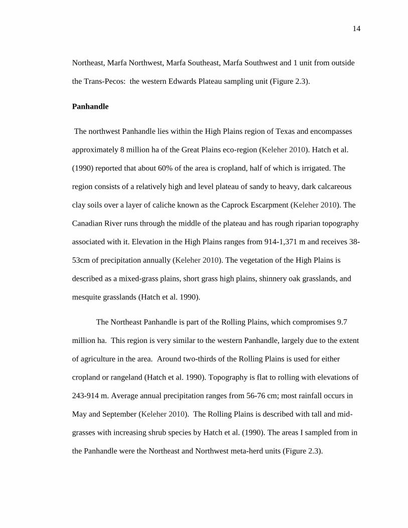
14

Northeast, Marfa Northwest, Marfa Southeast, Marfa Southwest and 1 unit from outside

the Trans-Pecos: the western Edwards Plateau sampling unit (Figure 2.3).

Panhandle

The northwest Panhandle lies within the High Plains region of Texas and encompasses

approximately 8 million ha of the Great Plains eco-region (Keleher 2010). Hatch et al.

(1990) reported that about 60% of the area is cropland, half of which is irrigated. The

region consists of a relatively high and level plateau of sandy to heavy, dark calcareous

clay soils over a layer of caliche known as the Caprock Escarpment (Keleher 2010). The

Canadian River runs through the middle of the plateau and has rough riparian topography

associated with it. Elevation in the High Plains ranges from 914-1,371 m and receives 38-

53cm of precipitation annually (Keleher 2010). The vegetation of the High Plains is

described as a mixed-grass plains, short grass high plains, shinnery oak grasslands, and

mesquite grasslands (Hatch et al. 1990).

The Northeast Panhandle is part of the Rolling Plains, which compromises 9.7

million ha. This region is very similar to the western Panhandle, largely due to the extent

of agriculture in the area. Around two-thirds of the Rolling Plains is used for either

cropland or rangeland (Hatch et al. 1990). Topography is flat to rolling with elevations of

243-914 m. Average annual precipitation ranges from 56-76 cm; most rainfall occurs in

May and September (Keleher 2010). The Rolling Plains is described with tall and mid-

grasses with increasing shrub species by Hatch et al. (1990). The areas I sampled from in

the Panhandle were the Northeast and Northwest meta-herd units (Figure 2.3).

15

Figure 2.3 Pronghorn meta-herd units in Texas as delineated by Texas Parks and

Wildlife Department for disease analysis.

16

METHODS

Trans-Pecos Sampling

Pronghorn were sampled during the 9-day, buck only, hunting season using hunter

harvested animals to evaluate mineral levels (copper and selenium) in blood and liver

samples. The blood was also tested for BTV and EHD.

Upon harvest, blood samples were collected from pronghorn via cardiac puncture

in non‐additive tubes and then transported to Sul Ross State University (SRSU). Within

24 h of collection, blood was centrifuged and serum samples were extracted and frozen.

Sera were analyzed by the Texas Veterinary Medical Diagnostic Laboratory (TVMDL) in

College Station, Texas. A measurement of copper (Cu), as well as the presence of

antibodies against BTV and EHD were analyzed using serum. To test for copper levels in

serum, TVMDL used Flame Atomic Absorption Spectrometry (FAAS). Using this

method, either an air/acetylene or a nitrous oxide/acetylene flame is used to evaporate the

solvent and dissociate the sample into its component atoms. When light passes through

the cloud of atoms, the atoms of interest absorb the light from the lamp. This is measured

by a detector, and used to calculate the concentration of that element in the original

sample (Principle of atomic absorption 2013). To test for BTV and EHD, the lab used 2

different tests known as a Polymerase Chain Reaction (PCR) and an agar gel

immunodiffusion (AGID). A PCR focuses on a segment of DNA and makes billions of

copies. The method relies on thermal cycling, and short DNA fragments known as

primers, which enable selective and repeated amplification (Genetics Home Reference

2013). An AGID is used to detect antibodies against selected bacteria and viruses. An

17

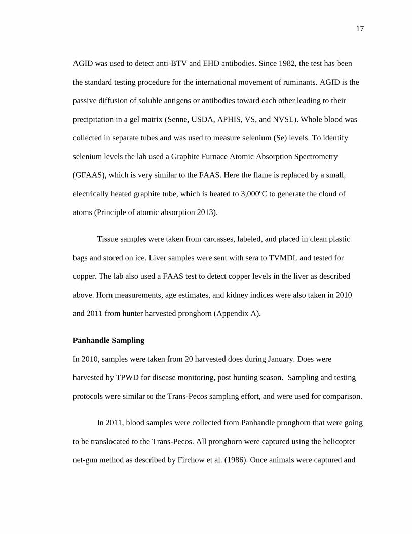
AGID was used to detect anti-BTV and EHD antibodies. Since 1982, the test has been

the standard testing procedure for the international movement of ruminants. AGID is the

passive diffusion of soluble antigens or antibodies toward each other leading to their

precipitation in a gel matrix (Senne, USDA, APHIS, VS, and NVSL). Whole blood was

collected in separate tubes and was used to measure selenium (Se) levels. To identify

selenium levels the lab used a Graphite Furnace Atomic Absorption Spectrometry

(GFAAS), which is very similar to the FAAS. Here the flame is replaced by a small,

electrically heated graphite tube, which is heated to 3,000ºC to generate the cloud of

atoms (Principle of atomic absorption 2013).

Tissue samples were taken from carcasses, labeled, and placed in clean plastic

bags and stored on ice. Liver samples were sent with sera to TVMDL and tested for

copper. The lab also used a FAAS test to detect copper levels in the liver as described

above. Horn measurements, age estimates, and kidney indices were also taken in 2010

and 2011 from hunter harvested pronghorn (Appendix A).

Panhandle Sampling

In 2010, samples were taken from 20 harvested does during January. Does were

harvested by TPWD for disease monitoring, post hunting season. Sampling and testing

protocols were similar to the Trans-Pecos sampling effort, and were used for comparison.

In 2011, blood samples were collected from Panhandle pronghorn that were going

to be translocated to the Trans-Pecos. All pronghorn were captured using the helicopter

net-gun method as described by Firchow et al. (1986). Once animals were captured and

18

restrained, blood samples were drawn from the jugular vein. Two tubes were collected

for serum testing and 1 tube was collected for whole blood testing. Blood was centrifuged

and serum samples were again extracted and frozen. Identical blood tests were conducted

to allow for comparison between the 2 populations. In addition to the other blood test, a

standard Serum Augglutination Test (SAT) was conducted to test for Brucellosis. SAT is

a serological test that is used to detect the presence of brucellosis antibodies.

Statistical Analysis-The program IBM SPSS Statistics 19 was used for all statistical

analysis. All data was first tested for normality using Kolmogorov-Smirnov test of

normality (Zar 2010). For the Trans-Pecos region, 3 years of data were compared

between years, for serum copper, liver copper, and whole blood selenium levels. For the

Panhandle region, 2 years of data were compared between years, for serum copper and

whole blood selenium levels. The Panhandle region only had 1 year of samples for liver

copper levels; therefore, comparisons between years were not possible. All 3 variables

(serum copper levels, liver copper levels, whole blood selenium levels) were compared

across regions (Trans-Pecos, Panhandle) using a t-test. An analysis of variance

(ANOVA) was used to compare serum copper levels and whole blood selenium levels

across years for the Trans-Pecos. A t-test was used for comparison for the Panhandle

since there were only 2 years of data for serum copper and whole blood selenium levels.

A Tukey’s HSD post hoc test was then used to compare years when a difference was

detected. The liver copper levels were non-normal; therefore, nonparametric tests were

used for comparisons (Conover and Iman 1980). A Kruskal-Wallis test for independent

samples was used to compare between years for all liver copper levels for the Trans-

19

Pecos region (Zar 2010). A Mann-Whitney U test for independent samples was used to

compare liver copper levels across region, only for the year (2010) when both regions

were sampled.

RESULTS

Trans-Pecos-I collected 102 samples from hunter-harvested pronghorn in October of

2009, 95 samples in 2010, and 49 samples in 2011 to evaluate the occurrence of BTV,

EHD, and copper and selenium levels. All samples collected in the Trans-Pecos were

bucks harvested during the 9-day hunting season.

Testing for BTV and EHD was not conducted in 2009. The prevalence of BTV

was 96% in 2010, and 100% in 2011. The prevalence of EHD was 92% in 2010, and 93%

in 2011 (Table 2.1). Average copper levels from blood sera were 0.68 ppm (SE = 0.03) in

2009, 0.72 ppm (SE = 0.02) in 2010, 0.84 ppm (SE = 0.03) in 2011. Average copper

levels from the liver in 2009 were 7.80 ppm (SE = 0.37), 8.56 ppm (SE = 0.37) in 2010,

and 7.91 ppm (SE = 0.41) in 2011. Average selenium levels from whole blood averaged

133.80 ppb (SE = 9.27) in 2009, 174.06 ppb (SE = 8.86) in 2010, and 212.10 ppb (SE =

14.88) in 2011 (Table 2.1).

Panhandle-Samples were collected in January 2010 from 20 harvested pronghorn

throughout 5 different herd units in the Panhandle. Average copper levels from the liver

averaged 10.41 ppm (SE = 0.44) and copper levels from blood samples averaged 0.40

ppm (SE = 0.03). Average selenium levels from blood samples averaged 164.4 ppb (SE =

12.80).

20

Table 2.1 Average disease and mineral levels from hunter-harvested pronghorn taken

from Trans-Pecos, Texas, USA, 2009-2011.

2009

(n = 102)

2010

(n = 95)

2011

(n = 49)

EHD Prevalence (%) - 92 93

BTV Prevalence (%) - 96 100

Cu Liver (ppm) 7.8 8.56 7.91

Cu Serum (ppm) 0.68 0.72 0.84

Se Blood (ppb) 133.80 174.06 212.10

21

In February 2011, I collected blood samples from 200 captured pronghorn that

were to be translocated to the Trans-Pecos. Blood was drawn and results were provided

from almost all animals captured in February 2011 (n = 195 for Cu; n = 196 for Se). The

prevalence of BTV was 87%, whereas the prevalence of EHD was 50.5% (Table 2.2).

Average copper and selenium levels were 0.74 ppm (SE = 0.01) and 208.43 ppb (SE =

3.15), respectively. In addition, 198 samples were tested for brucellosis in 2011 with all

resulting in negatives.

Statistical Analysis- When comparing serum copper levels across years (2009, 2010,

2011) for the Trans-Pecos there was a significant difference (P < 0.001, F = 8.227, df =

2). Serum copper levels in 2011 were different than levels in 2009 (P < 0.001) and levels

in 2010 (P = 0.006). There was no difference in serum copper levels between 2009 and

2010 (P = 0.346). For the Panhandle, there was also a difference (P < 0.001, t = -11.196)

between 2010 and 2011 serum copper levels. Serum copper levels were also compared

between regions (Trans-Pecos, Panhandle), but no difference was documented (P =

0.199, t = 1.287).

Whole blood selenium levels were compared across years (2009, 2010, 2011) for

the Trans-Pecos and there was a difference (P < 0.001, F = 10.19, df = 2). Selenium

levels for 2009 were different than levels in 2010 (P = 0.028), and levels in 2011 (P <

0.001). Selenium levels for 2010 were also different from levels documented in 2011 (P

= 0.035). The Panhandle also had a difference (P < 0.001, t = -3.588) between years

(2010, 2011). When comparing whole blood selenium levels between regions (Trans-

Pecos, Panhandle) there was a difference (P < 0.001, t = -4.767).

22

Table 2.2 Average disease prevalence and mineral levels from hunter-harvested and

captured pronghorn taken from Panhandle, Texas, USA, 2010-2011.

Averages 2010a

(n = 20)

2011b

(n = 200)

EHD Prevalence (%) - 50.5

BTV Prevalence (%) - 87

Cu Liver (ppm) 10.41 -

Cu Serum (ppm) 0.40 0.74

Se Blood (ppb) 164.4 208.43

a Harvested

b Captured

23

Liver copper levels were only compared across years for the Trans-Pecos since only 1

year of samples were collected from the Panhandle region. Liver copper levels were the

same (P = 0.433, X2 = 1.675, Df = 2) for all 3 years (2009, 2010, 2011) in the Trans-

Pecos. When comparing liver copper levels across regions, levels were only compared for

the year (2010) both regions were sampled. There was a difference (P = 0.001, U =

527.5) between regions when comparing liver copper levels in 2010.

DISCUSSION

BTV and EHD have affected pronghorn populations in other regions of the country and

can be very detrimental to a population in some cases. Large die-offs were recorded in

Wyoming, which were linked to BTV (Thorne et al. 1988). Kistner et al. (1975) found

that BTV or EHD was the cause for 2 captive pronghorn to die in Oregon. Allen (1874)

described the largest die-off of pronghorn between the Yellowstone and Missouri rivers

during the summer of 1873, which could have been BTV. However, these diseases do not

appear to be a major issue in pronghorn in Texas. I collected samples for 3 years in the

Trans-Pecos and recorded a very high prevalence for BTV and EHD.

Based on my results, 98% of pronghorn in this region had come in contact with,

and showed titers for BTV. I also reported 91% of pronghorn in this region showed titers

for EHD. Antibodies for BTV and EHD are normally found at a higher prevalence in

southern populations (O’Gara 2004). Stauber et al. (1980) tested 104 adults and 42 fawns

in 3 populations in southeastern Idaho and found no reactors to BTV or EHD. Jochim and

Chow (1969) performed a serological survey in 1963, he found evidence that 8 (8%) of

24

96 pronghorn from Wyoming and 34 (35%) of 97 pronghorn from Colorado had come in

contact with BTV. Tests conducted in Nebraska, found evidence that 92 and 103 (27%

and 30%, respectively) out of 339 pronghorn had positive tests for BTV and EHD

(Johnson et al. 1986). In Arizona, 226 (78.5%) of 288 pronghorn tested positive to

exposure to BTV (Heffelfinger and Oldin 1997, Heffelfinger et al. 1999). Pronghorn

from the Trans-Pecos and other southern populations appear to have a higher prevalence

of titers to BTV and EHD than do northern populations. Immunity may be implied by the

presence of antibody titers (O’Gara 2004). The year I sampled for diseases in the

Panhandle, I saw lower prevalence for EHD, where 50.5% of animals showed titers

compared to the Trans-Pecos. The average prevalence for BTV was slightly lower in the

Panhandle, where 87% of animals showed titers.

Selenium and copper are both important to pronghorn for overall health and

reproduction (Flueck and Smith-Flueck 1990). Dunbar et al. (1999) reported that

deficiencies of minerals are responsible for decreased animal condition, fertility,

productivity, as well as increased mortality. When comparing mineral levels from

pronghorn populations in the Panhandle to those populations in the Trans-Pecos, I

concluded that copper levels in the liver and selenium whole blood levels were not the

same. The Trans-Pecos region exhibited lower copper levels in the liver and selenium

whole blood levels, which may be part of the reason this area is experiencing such low

productivity. There is very little data available for normal blood and serum levels of wild

ungulates so determining what these levels mean in pronghorn is very difficult (Dunbar et

25

al. 1999). Therefore, I cannot say that one population has high or low copper and

selenium levels or if both populations are normal.

Normal levels of copper in the liver for sheep, cattle, and deer range from 25 to

100 ppm (Dunbar et al. 1999). Though both populations appear to be deficient in copper

when compared to these numbers, the Panhandle population was higher than the Trans-

Pecos region. Although, I only have 1 year (2010) of liver copper levels for the

Panhandle, copper levels in the liver were considerably higher than the same year I

collected samples in the Trans-Pecos. A normal level for copper serum for most

ruminants is 0.7-1.2 ppm (Dunbar et al. 1999), which shows both regions appear to have

marginal levels of copper. There was no difference between the pronghorn populations

between regions (Trans-Pecos, Panhandle). Although normal levels of copper and

selenium for pronghorn are unknown at this point, I believe that both the Trans-Pecos and

the Panhandle regions exhibit marginal mineral levels in pronghorn.

This study was established to determine some of the leading factors causing a

pronghorn decline in the Trans-Pecos. Minerals levels and diseases have both been

known to cause pronghorn populations to decline. BTV and EHD both have larger

impacts in northern populations where titers for these diseases are lower. Since

pronghorn in the Trans-Pecos show a very high prevalence for BTV and EHD, I believe

that this data places more emphasis on mineral levels and draws less attention to these

diseases as major contributors to this population’s decline.

26

Management Implications

Unlike other ungulates, little information is known about normal mineral levels in

pronghorn since they do not do well in captivity, which is used to help establish baseline

levels of trace minerals. Copper and selenium both play an important role in pronghorn

production. Low mineral levels in animals could be a reflection of diet, since minerals

levels are diet dependent. Diseases such as the BTV and EHD are both naturally

occurring throughout much of pronghorn range. Pronghorn in the Trans-Pecos show very

high prevalence for both diseases; therefore, these diseases have little effect on the

population. Managers could supplement pronghorn with loose minerals and/or mineral

blocks around waters and other areas pronghorn frequently use. Pronghorn have been

known to use mineral supplements when they are available. Minerals are tied to

productivity in pronghorn so making mineral supplements available for pronghorn could

increase their health. Managers should also implement a conservative grazing plan and

modify fences, which will allow pronghorn to move freely across the landscape and attain

trace minerals from native vegetation. Any pronghorn mortalities found should be

reported to state or local wildlife agencies, so proper testing and documentation can be

handled and any diseases such as BTV and EHD can be managed.

LITERATURE CITED

Allen, J. A. 1874. Notes on the natural history of portions of Dakota and Montana

territories. Proceedings of the Boston Social of Natural History 17:33-85.

27

Buechner, H. K. 1950. Life history, ecology, and range use of the pronghorn

antelope in Trans‐Pecos of Texas. American Midland Naturalist 43:257–354.

Canon, S. K., and F. C. Bryant. 1997. Home ranges of pronghorn in the Trans‐Pecos

region of Texas. Texas Journal of Agricultural and Natural Resources 10:87–92.

Church, D. G ., and W. G. Pond. 1978. Basic animal nutrition and feeding. Albany Print.

Albany, Oregon, USA.

Conover, W. J., and R. C. Iman. 1980. Rank transformations as a bridge between

parametric and nonparametric statistics. American Statistician 35:124-129.

Dunbar, M. R., R. Velarde, M. A. Gregg, and M. Bray. 1999. Health evaluation of a

pronghorn antelope population in Oregon. Journal of Wildlife Diseases 35:496-

510.

Flueck, W. T., and J. M. Smith-Flueck. 1990. Selenium deficiency in deer: The effect of

a declining selenium cycle? Transactions of the Congress of the International

Union of Game Biologists 19:292-301.

Firchow, K. M., M. R. Vaughan, and W. R. Mytton. 1986. Evaluation of the hand-held

net gun for capturing pronghorns. Journal of Wildlife Management 50:320-322.

Genetics Home Reference [GHR]. 2013. Your guide to understanding genetic conditions.

Polymerase chain reaction. <http://ghr.nlm.nih.gov/glossary=polymerase

chainreactionpcr>. Accessed 4 June 2013.

Gray, S. S. 2012. Big game research and surveys: Pronghorn harvest recommendations.

Federal Aid Project W-127-R-20. Texas Parks and Wildlife Department, Austin,

Texas, USA.

28

Harveson, L. A. Life history and ecology of pronghorn. Pages 1–4 in K. A. Cearly and

S. Nelle, editors. Pronghorn Symposium 2006. Texas Cooperative Extension,

College Station, Texas, USA.

Hatch, S. L., K. N. Gandhi, and L. E. Brown. 1990. Checklist to the vascular plants of

Texas. Publication MP‐1655, Texas Agricultural Experiment Station, Texas

A&M University, College Station, Texas, USA.

Heffelfinger, J. R., and R. J. Olding. 1996. Occurrence and distribution of blue tongue in

pronghorn antelope. P-R Performance Report, Project W-53-M-47. Arizona

Department of Game and Fish, Phoenix, Arizona, USA.

Heffelfinger, J. R., R. J. Olding, T. H. Noon, M. R. Shupe, and D. P. Betzer. 1999.

Copper/selenium levels and occurrence of bluetongue virus in Arizona pronghorn.

Proceedings of the Pronghorn Antelope Workshop 18:32–42.

Jochim, M. M., and T. L. Chow. 1969. Immunodiffusion of blue tongue virus. American

Journal of Veterinary Research 30:33-41.

Johnson, J. L., T. L. Barber, M. L. Frey, and G. Nason. 1986. Serosurvey for selected

pathogens in hunter-killed pronghorn in western Nebraska. Journal of Wildlife

Diseases 22:87-90.

Keleher, R. C. 2010. Genetic variation of pronghorn populations in Texas. Thesis, Sul

Ross State University, Alpine, Texas, USA.

Kistner, T. P., G. E. Reynolds, L. D. Koller, C. E. Trainer, and D. L. Eastman. 1975.

Clinical and serological findings on the distribution of blue tongue and epizootic

29

disease viruses in Oregon. Proceedings of the American Association of Veterinary

Laboratory Diagnosticians 18:135-147

Miller, M., S. Amsel, J. Boehm, and B. Gonzales. 2001. Presumptive copper deficiency

in hand-reared captive pronghorn (Antilocapra americana) fawns. Journal of Zoo

and Wildlife Medicine 32:373-378.

O’Gara, B. W., and J. D. Yoakum. 1992. Pronghorn management guides. Fifteenth

Biennial Pronghorn Antelope Workshop. Rock Springs, Wyoming, USA.

O’Gara, B. W. 2004. Diseases and parasites. Pages 299-336 in B. W. O’ Gara, and J. D.

Yoakum, editors. Pronghorn: Ecology and management. University Press of

Colorado, Boulder, Colorado, USA.

O’Hara, T. M., G. Carroll, P. Barboza, K. Muller, J. Blake, V. Woshner, and C. Willetto.

2001. Mineral and heavy metal status as related to a mortality event and poor

recruitment in a moose population in Alaska. Journal of Wildlife Diseases 37:509-

522.

Pittman, M. T. 1987. Mule deer reproduction. P‐R Report number 51‐W‐109‐R‐10,

Texas Parks and Wildlife Department, Austin, Texas, USA.

Principle of atomic absorption/emission spectroscopy. Atomic emission-the flame test.

<http://faculty.sdmiramar.edu/fgarces/LabMatters/Instruments/AA/AAS_Theory/

AASTheory.htm>. Accessed 4 June 2013.

Puls, R. 1994. Mineral levels in animal health diagnostic data, second edition. Sherpa

International, Clearbrook, British Columbia, Canada.

30

Senne, D. A., United States Department of Agriculture [USDA], Animal Plant Health

Inspection Service [APHIS], Veterinary Services [VS], and National Veterinary

Services Laboratories. Agar gel immunodiffusion (AGID) test principles and

techniques. < http://www.cfsph.iastate.edu/HPAI/resources/Presentations

/AGID%20Overview-D.Senne.pdf>. Accessed 4 June 2013.

Starkey, E. E., D. S. Decalesta, and G. W. Witmer. 1982. Management of Roosevelt elk

habitat and harvest. Transactions of the North American Wildlife Natural

Resource Conference 47:353-362.

Stauber, E. H., R. Autenrieth, O. D. Markham, and V. Whitbeck. 1980. A

seroepidemiologic survey of three pronghorn (Antilocapra americana)

populations in southeastern Idaho, 1975-1977. Journal of Wildlife Diseases

16:109-115.

Stoszek, M. J., W. B. Kessler, and H. Willmes. 1978. Trace mineral content of antelope

tissues. Proceedings from the Pronghorn Antelope Workshop, Jasper, Alberta,

Canada 8:156-161

Tarrant, B., L. A. Harveson, S. S. Gray, and K. A. Waldrup. 2010. Internal parasite

concentrations of pronghorn in Trans-Pecos, Texas. Proceedings from the

Pronghorn Workshop 24:112-118.

Thorne, E. T., E. S. Williams, T. R. Spraker, W. Helms, and T. Segerstrom. 1988.

Bluetongue in free‐ranging pronghorn antelope (Antilocapra americana) in

Wyoming: 1976 and 1984. Journal of Wildlife Diseases 24:113–119.

31

Waldrup, K. A., E. Collisson, S. E. Bentsen, C. K. Winkler, and G. G. Wagner. 1989.

Prevalence of erythrocytic protozoa and serologic reactivity to selected pathogens

in deer in Texas. Preventive Veterinary Medicine 7:49–58.

Zar, J. H. 2010. Biostatistical analysis. 5th

Edition. Pearson Prentice Hall, Upper Saddle

River, New Jersey, USA.

Zimmermann, T. J., J. A. Jenks, D. M. Leslie, Jr., and R. D. Neiger. 2008. Hepatic

minerals of white‐tailed and mule deer in the southern Black Hills, South Dakota.

Journal of Wildlife Diseases 44:341–350.

32

CHAPTER III: HAEMONCHUS-PRONGHORN INTERACTIONS IN TEXAS

Historically, pronghorn (Antilocapra americana) were distributed over approximately

two‐thirds of Texas including all areas west of the 97th meridian (Buechner 1950). Today

pronghorn populations are restricted to the Chihuahuan Deserts (Trans‐Pecos), High

Plains, Southwestern Tablelands, and Edwards Plateau ecoregions (Gray 2012).

Historically, the Trans‐Pecos supported approximately 60–70% of the state’s pronghorn,

with numbers reaching a high of about 17,000 animals during the wetter years of the

mid‐1980s (Tarrant et al. 2010).

In 2008, following an 8‐month drought in the Trans‐Pecos, Texas Parks and

Wildlife Department documented a significant die‐off of adult pronghorn where an

estimated 2,000–3,000 pronghorn succumbed in one of the most productive regions of

west Texas (e.g., Marfa Plateau; Tarrant et al. 2010). Given the relationship between

precipitation and pronghorn demography (Simpson et al. 2006), the 2008 die‐off was not

surprising. However, in 2009, biologists were not able to attribute the continued decline

to precipitation‐mediated variables alone. Specifically, the first half of 2009 brought

timely and abundant precipitation, which based on population trend data would have been

ideal habitat conditions with abundant forage (forbs and browse) and cover (perennial

grasses) for population recovery (Tarrant et al. 2010). Unfortunately, pronghorn did not

respond to the excellent habitat conditions and population productivity and abundance

fell even further. A mean fawn:doe ratio of 13:100 was recorded with a population

estimate of 6,000 animals (near record lows) in 2009 (Tarrant et al. 2010).

33

Haemonchus is one of the most highly prolific parasitic nematodes afflicting both

domestic and wild ruminants (McGhee et al. 1981, Newton and Munn 1999).

Haemonchus is known to cause deleterious effects to the animal, entire populations, and

animal wildlife industry (McGhee et al. 1981, Newton and Munn 1999). As a prolific

breeder, a single female worm produces about 10,000 eggs per day (Prichard 2001, Zajac

2006). This allows larvae to rapidly accumulate on pastures as the prepatent period

(length of time between infection of host and parasite maturity) is between 17 to 21 days

(Prichard 2001, Zajac 2006).

The life cycle of Haemonchus involves an adult female in the abomasum

ingesting a blood meal and laying eggs daily that are subsequently passed in the host’s

fecal material (Zajac 2006). Fecal material provides the eggs protection from

environmental conditions and optimal temperature and moisture for further development

(O’Conner et al. 2006). As the first‐stage larva forms and hatches from the egg, larvae

feed on bacteria and undergo 2 molts before reaching the infective third larvae stage (L3;

Zajac 2006). The optimal conditions for development of Haemonchus eggs into infective

larvae occur at 23°C and 70% fecal moisture content, yet can still occur at a range

between 10°C to 36°C (O’Conner et al. 2006, Zajac 2006). However, O’Conner et al.

(2006) noted that development can be accelerated if temperatures and moisture content

increased or decreased when conditions are less than optimal. Once L3 stage

development is complete and in the subsequent presence of rain, larvae make their way

out of the fecal material and migrate onto forage to be later ingested (O’Conner et al.

2006, Zajac 2006). L3 stage Haemonchus are considerably less susceptible to

34

unfavorable climatic conditions and this is attributed to their migratory behavior. The

population size of Haemonchus on a pasture is considered much greater than the number

of parasites within a single ruminant (Prichard 2001). As the infective larvae are ingested,

Haemonchus molts once more into the L4 stage and shed their protective L3 stage larvae

sheath in the abomasum.

Severe outbreaks of Haemonchus infection are most often reported to occur

during warm summer rains, among young, non‐immune animals, immunocompromised

adult animals, or animals exposed to high levels of parasites (Zajac 2006). Because of the

prevalence in many ruminants and reproductive success in tropical and sub‐tropical areas,

or regions with summer‐dominant rainfall, Haemonchus encompasses an enormous

environmental range of suitable habitat (O’Conner et al. 2006).

Although a majority of all grazing ruminants are infected with stomach worms,

only sub‐clinical and clinical effects of disease are observed under heavy worm burdens.

Clinical signs of disease involve weight loss, diarrhea, “bottle jaw” (e.g., edema, or fluid

accumulation under the jaw), protein loss across the gut wall, anemia, weakness, and

death (McGhee et al. 1981, Simpson 2000, Zajac 2006). Haemonchus has been

responsible for numerous infections on a wide variety of ruminants, commonly and most

often reported in domestic ruminants such as sheep, goats, and cattle (McGhee et al.

1981, Lichtenfels et al. 1994, Zajac 2006). Haemonchus has also been documented in

wild ruminants such as white‐tailed deer (Odocoileus virginianus), bighorn sheep (Ovis

canadensis), and pronghorn (Allen et al. 1959, McGhee et al. 1981, Lichtenfels et al.

35

1994, Newton and Munn 1999). Bever (1957) described parasitism in pronghorn and

field methods to measure the parasitic load. Research conducted during the late 1960s in

the Trans‐Pecos documented the presence of Haemonchus (Hailey 1968), but were not

thought to be of concern. Investigators concluded the pronghorn herds were clean of

parasites and diseases because of the dry climate, which helps to prevent the spread of

diseases (Hailey 1968). Because Haemonchus is found in livestock and wildlife there is

potential for cross‐transmission.

The ability for Haemonchus to infect a wide variety of hosts with little geographic

impediment allows for great genetic diversity, as well as a high rate of mutation (Prichard

2001). Furthermore, in combination with the use of a broad‐spectrum and frequent use of

chemical treatment, widespread resistance in Haemonchus populations to anthelmintics

exists. Chronic problems in the sheep and goat industry have emerged because of the

increased resistance of Haemonchus to wormers and other treatments. The sheep industry

estimates a loss of >$100,000,000/year from the treatment of Haemonchus (Newton and

Munn 1999).

Therefore, the infection of pronghorn in west Texas with Haemonchus poses a

series of concerns for the population and future management. However, further research,

monitoring, and investigation of host‐parasite interaction is imperative to make sound

decisions on methods of control or prevention to be utilized. I initiated a study to

determine how Haemonchus interact with pronghorn and to better understand what

effects this parasite has on pronghorn as the host. I wanted to document infection rates for

36

pronghorn in the Trans-Pecos and compare to other populations. I predicted (1) worm

counts in the abomasums will be positively correlated to fecal egg counts, and (2)

Haemonchus will be negatively correlated with pronghorn fawn recruitment in the Trans-

Pecos.

STUDY AREA

In the Chihuahuan Desert (Trans-Pecos) ecoregion, pronghorn principally reside in the

Chihuahuan Desert Grassland ecoregion, which ranges in elevation from 1,060–1,680 m

and receives 25–46 cm of annual precipitation. Rainfall is from monsoonal events

peaking during the months of July–September. The average growing season is about

190–240 days. Dominant plant species include black grama (Bouteloua eriopoda ), blue

grama (Bouteloua gracilis), and sideoats grama (Bouteloua curtipendula), bush muhly

(Muhlenbergia porteri), beargrass (Nolina arenicola), tobosa grass (Pleuraphis mutica),

and galleta (Pleuraphis jamesii) with scattered creosotebush (Larrea tridentata), tarbush

(Flourensia cernua), acacias (Acacia spp.), yucca (Yucca spp.), and cacti (Opuntia spp.)

(Griffith et al. 2007). Land use practices vary across the Trans-Pecos, but most

rangelands are used for livestock grazing or wildlife enterprises (Harveson 2006). Seven

disease sampling units have been delineated in the Trans-Pecos where I initiated

surveillance (Figure 2.3).

Panhandle pronghorn populations are found in the High Plains and Southwestern

Tablelands ecoregions with most occurring in the Canadian-Cimarron High Plains,

Rolling Sand Plains, and Canadian-Cimarron Breaks ecoregions. These ecoregions are

37

characterized by short to mid-grass vegetation communities with plant species such as

gramas, buffalograss (Buchloe dactyloides), bluestems (Andropogon, Bothriochloa,

Schizachyrium spp.), sand dropseed (Sporobolus cryptandrus), Havard shin oak (Quercus

havardii), sand sagebrush (Artemisia filifolia), yucca, mesquite (Prosopis glandulosa),

skunkbush sumac (Rhus trilobata), and Chickasaw plum (Prunus angustifolia) being the

most common. In addition, large areas of croplands dominate the landscape with a

scattering of playa lakes. Elevations vary from 700-1,370 meters. Average rainfall is

between 40-58 centimeters and is more bimodal than the Chihuahuan Desert ecoregion

with the greatest amount of precipitation falling in the spring and fall months. The

average growing season is from 170–200 days (Griffith et al. 2007, Keleher 2010).

METHODS

Trans-Pecos-I coordinated the collection of hunter harvested pronghorn samples with

landowners, outfitters, and hunters across the region. Much of the ground work for this

was done with the help of the local Texas Parks and Wildlife Department district

biologists. In many cases, trained researchers accompanied hunters to ensure samples

were taken properly. In 2009, 2010, and 2011 abomasum samples were collected from

harvested pronghorn during evisceration. Upon evisceration, a string was used to tie off

both ends of the abomasum. After knots were secured, the abomasum was dissected and

removed from the body cavity. Abomasums were placed in clean plastic bags, labeled,

and transported on ice to the lab. Upon arrival to the lab, abomasums were cut 2laterally

and contents were rinsed carefully into a collection vessel. During 2009, abomasums

were quantified using a sampling technique, where all the contents of an abomasum were

38

washed in a container using water. Contents of the wash were gently stirred and 200 ml

of fluid content was collected off the surface. All worms were then counted in the 200 ml

and that total was then extrapolated to the rest of the solution to estimate a total parasite

load for that animal. In 2010 and 2011 a total count was applied to each abomasum to

ensure accuracy. All nematodes found in the supernatant and abomasums were counted

and stored in alcohol (or formalin) for species identification.

Fecal samples were extracted directly from the rectum of all hunter‐harvested

pronghorn. Eight to 12 pellets were placed in a plastic bag, stored on ice, and transported

to the lab. If samples were stored longer than 24 h, they were vacuumed sealed, to help

prevent eggs from hatching. Fecal samples were analyzed using the McMaster’s fecal

flotation technique as described by Burk and Rossano (2011) to determine the amount of

nematode eggs/gram of feces.

To determine if parasite loads were negatively correlated with fawn recruitment

as predicted, I compared worm counts to fawn crops, across each meta-herd unit using

Spearman’s rho correlation test for non-normal data (Zar 2009). Both worm loads and

fawn crops were averaged across meta-herd units for comparison. I used worm load data

from the fall and compared that to the TPWD fawn crop averages for the following

spring (e.g., 2010 worm loads vs. 2011 fawn crops) (Gray 2012). Texas Parks and

Wildlife Department flew aerial surveys during the months of June and July annually and

this data was used to estimate fawn crops for the different meta-herd units.

39

Other wildlife species sampled in the Trans-Pecos.—In 2010, I was also able to

collect samples from Barbary sheep (Ammotragus lervia), mule deer (Odecoileus

hemionus), and cattle from the Trans-Pecos region. This allowed me to compare parasite

loads in pronghorn to other ruminants within the same region.

Panhandle-Samples were collected in January 2010 from 20 harvested pronghorn does

throughout 5 different herd units in the northeast and northwest Texas Panhandle. In

February 2011, I collected fecal samples from 178 captured pronghorn that were later

translocated to the Trans-Pecos.

Species Identification and Drug Resistance-Because a variety of nematodes are

common in wild ungulates correct identification of Haemonchus may be suspect (O’Gara

2004). Therefore, I preserved samples of the parasitic community in formalin for

identification by the USDA’s Animal Parasitic Diseases Laboratory in Beltsville,

Maryland. I sent samples to the lab where they used DNA and molecular data to compare

Haemonchus found in Trans-Pecos pronghorn to other known species of Haemonchus

(personal communication, Hoberg, USDA Animal Parasitic Disease Laboratory,

Beltsville, MD).

To better understand the origin and possible host of Haemonchus spp., I sent fecal

samples off to the University of Georgia’s College of Veterinary Medicine to have the

DrenchRite® Larval Development Assay (LDA) test performed (personal

communication, R. Kaplan, The University of Georgia, College of Veterinarian

Medicine, Department of Infectious Diseases, Athens, GA). LDA is an in vitro test for

40

the detection of anthelmintic resistance in the major gastrointestinal nematode parasites

infecting small ruminants (sheep, goats, llama, alpaca, etc). LDA evaluates the resistance

to benzimidazole (e.g., Valbazen, Panacur, Safeguard), levamisole (e.g., Totalon,

Levasol, Prohibit), and avermectin/milbemycin (Ivomec, Cydectin). Nematode resistance

to all drug classes listed above is tested for in each assay from a single pooled fecal

sample. For LDA, nematode eggs are isolated from feces and placed into the wells of a

microtiter plate containing growth media and anthelmintic. The concentration of

anthelmintic required to block development of nematode larvae is related to the

effectiveness of the drug in the animal.

Statistical Analysis-The program IBM SPSS Statistics 19 was used for all statistical

analysis. All data was first tested for normality using Kolmogorov-Smirnov test of

normality (Zar 2010). Worm counts and fecal egg count data were non-normal so

nonparametric tests were used for analysis. A Spearman’s Rho correlation test (Conover

and Iman 1980, Zar 2010) was used to evaluate the relationship of worm counts in

abomasums and fecal egg counts for 2 years (2010, 2011) in the Trans-Pecos region. A

Spearman’s Rho test was also used to evaluate the relationship between worm counts in

abomasums and fawn crops (fawns/100 does) in the Trans-Pecos for 3 consecutive years

(2009, 2010, 2011). An independent samples Kruskal-Wallis test (Zar 2010) was used to

compare worm counts and fecal egg counts for the Trans-Pecos region across years.

Pairwise comparisons were then used to determine which years differed for both worm

counts and fecal egg counts. For the Panhandle region, only 1 year of worm count data

was collected, so yearly comparisons were not possible. A Mann-Whitney U test

41

(Conover and Iman 1980) for independent samples was used to compare pronghorn fecal

egg counts by season (Fall/Winter, Summer) for 2011 in the Panhandle region (Zar

2010). For comparisons of worm counts and fecal egg counts between regions (Trans-

Pecos, Panhandle) an independent samples Mann-Whitney U test was used. When

comparing worm counts and fecal egg counts of other species (Barbary sheep, mule deer)

to pronghorn in the Trans-Pecos for 2010, independent samples Kruskal Wallis test was

used. Pairwise comparisons were then used to determine which species differed. In the

summer of 2011, fecal samples were collected from cattle and pronghorn in the Trans-

Pecos and a Mann-Whitney U test for independent samples was used for comparison.

RESULTS

Trans-Pecos-I obtained 102 abomasum samples from pronghorn in 2009, 95 samples in

2010, and 49 samples in 2011. Average prevalence rate of barber pole worm was 94%,

that is 201 of the 215 samples that were analyzed had barber pole worms. In 2009, the

average number of worms/pronghorn was 551 (SE = 70.06) and ranged from 0 to 4,080

worms/animal. The average in 2010 was 268 (SE = 44.83) worms, which was 44% less

than the average in 2009, but parasite loads still ranged from 0 to 3,145. In 2011, worm

loads ranged from 0 to 2,507 and pronghorn averaged 381 (SE = 83.67) worms/animal

(Table 3.1).

Fecal egg counts for 2010 and 2011 averaged 1,267 (SE = 190.33) and 1,053 (SE

= 194.52) eggs/gram, respectively. Fecal egg counts for the summer of 2011 averaged

1,389 (SE = 260.68) eggs/gram and 167 (SE = 43.69) eggs/gram in the summer of 2012.

42

Table 3.1 Comparison of average number of Haemonchus worms and fecal egg count

averages in Trans-Pecos and Panhandle, Texas, USA, 2009-2012.

Region

Species

n

Season-Year

Abomasum

Worm

Counts

Fecal Egg

Counts-

Eggs/Gram

Trans-Pecos

Pronghorn

89c

Fall-2009d

551

-

Pronghorn

86 a, 91b

Fall-2010d

268

1,267

Mule Deer

20 a, 18b

Fall-2010d

4

15

Barbary Sheep

14 a, 13b

Fall-2010d

45

200

Pronghorn

63c

Summer-2011f

-

1,389

Cattle

15c

Summer-2011f

-

27

Pronghorn

42 a, 45b

Fall-2011d

381

1,053

Pronghorn

27c

Summer-2012f

-

167

Panhandle

Pronghorn

17c

Fall-2009d

90

-

Pronghorn

20c

Summer-2011f

-

608

Pronghorn

178c

Fall-2011e

-

117

a Abomasum worm count sample size

b Fecal egg count sample size

c Sample size for both counts

d Hunter harvested samples

e Capture samples

f Field samples

43

Other wildlife species sampled in the Trans-Pecos.—Fifteen samples were collected from

Barbary sheep in 2010, which averaged 45 (SE = 25.26) worms/abomasum, and the fecal

egg counts averaged 200 (SE = 106.67) eggs/gram. Twenty-four samples were collected

from mule deer, which averaged 4 (SE = 2.84) worms/abomasum with fecal egg counts

averaging 15 (SE = 10.94) eggs/gram. A total of 15 fecal samples was collected from

cattle from 3 different ranches and the fecal egg counts averaged 27 (SE = 10.76)

eggs/gram.

Panhandle- In 2010, the average worm load was 90 (SE = 25.99) worms/pronghorn for

the 20 does harvested in January. In 2011, fecal egg counts averaged 117 (SE = 28.93)

eggs/gram for the captured pronghorn. During summer 2011, fecal samples were

collected from pronghorn in the northern Panhandle and they averaged 608 (SE = 211.46)

eggs/gram (Table 3.1).

Statistical Analysis-For the Trans-Pecos region worm counts and fecal egg counts were

correlated in 2010 (rs = 0.902, P < 0.001) and in 2011 (rs = 0.915, P < 0.001) (Conover

and Iman 1980) (Figure 3.1). Worm loads of fall 2009 were correlated to the fawn crops

of spring 2010 (rs = -0.865, P = 0.012), but were not correlated in subsequent years

(Figure 3.2). I found insignificant correlations when comparing worm loads of fall 2010

to the fawn crops of spring 2011 (rs = -0.143, P = 0.760), and when comparing worm

loads of fall 2011 to the fawn crops of spring 2012 (rs = -0.43, P = 0.397) (Conover and

Iman 1980) (Figure 3.2).

In the Trans-Pecos, there was a difference (P = 0.002, X2 = 12.608, Df = 2) in

worm counts in pronghorn when compared across years (2009, 2010, 2011). Worm

44

0

500

1000

1500

2000

2500

3000

3500

0 2,000 4,000 6,000 8,000 10,000 12,000

Wo

rms

Fecal Egg Counts

A

(rs = 0.902, P < 0.001)

0

500

1,000

1,500

2,000

2,500

3,000

3,500

0 2,000 4,000 6,000 8,000 10,000 12,000

Wo

rms

Fecal Egg Counts

B

(rs = 0.915, P < 0.001)

Figure 3.1 Relationship between Haemonchus worm counts in abomasums and fecal egg

counts for 2010 (A) and 2011 (B) in Trans-Pecos, Texas, USA.

45

0

500

1000

1500

2000

0 20 40 60

Worm

s

Fawn Crop

A

(rs = -0.865, P = 0.012)

0

500

1000

1500

2000

0 20 40 60

Worm

s

Fawn Crop

B

(rs = -0.143, P = 0.760)

0

500

1000

1500

2000

0 20 40 60

Worm

s

Fawn Crop

C

(rs = -0.43, P = 0.397)

Figure 3.2 Relationship between Haemonchus worm loads and subsequent pronghorn

fawn crops for 2009 (A), 2010 (B), and 2011 (C) in Trans-Pecos, Texas, USA.

46

counts in 2009, were different (P = 0.003) than worm counts in 2010, but were similar (P

= 0.151) to worm counts in 2011. Years 2010 and 2011 were also similar (P = 0.451)

when comparing worm counts in pronghorn. When comparing fecal egg counts in the

Trans-Pecos between years (2010, 2011, 2012) there was a difference (P < 0.001, X2 =

19.339, df = 2). There was no difference (P = 0.579) in fecal egg counts between 2010

and 2011. Fecal egg counts in 2012 differed from 2010 (P < 0.001) and 2011 (P = 0.001).

In the Panhandle region, only 1 year of samples were collected for worm counts

so no yearly comparisons were conducted. Fecal egg counts were collected during 2

different time periods (winter, summer) for 2011. When comparing fecal egg counts

between seasons, I documented a difference (P = 0.009, U = 1178.5).

Panhandle worm counts and fecal egg counts were lower than Trans-Pecos

estimates. I found a difference when comparing worm counts (P = 0.041, U = 501.5) and

fecal egg counts (P < 0.001, U = 5365.5) between the Trans-Pecos and the Panhandle

regions.

Other species were also sampled in the Trans-Pecos for comparisons to

pronghorn. In 2010, pronghorn, Barbary sheep, and mule deer samples were collected

and a difference was found when comparing worm counts (P < 0.001, X2

= 51.254, df =

2) and fecal egg counts (P < 0.001, X2 = 42.669, df = 2) between the 3 species. Pronghorn

worm counts were different from both Barbary sheep (P = 0.004), and mule deer (P <

0.001). Mule deer and Barbary sheep had similar wrom counts (P = 0.623). Pronghorn

fecal egg counts also differed from Barbary sheep (P = 0.003), and mule deer (P <

47

0.001). Barbary sheep and mule deer fecal egg counts also differed (P = 0.006). In the

summer of 2011, cattle fecal samples were collected in the Trans-Pecos for fecal egg

count comparisons to pronghorn and again I documented a difference (P < 0.001, U =

157.5).

Species Identification and Drug Resistance-Samples sent to the USDA’s Animal

Parasitic Diseases Laboratory in Beltsville, Maryland, showed that pronghorn were

carrying more than one species of Haemonchus. The laboratory reported H. contortus and

H. placei in the pronghorn samples. The lab also reported mixed infections of these

species in some hosts, and indicated that there may be evidence for the occurrence of

hybrids of these species based on structural characteristics of the adult worms.

As for drug resistance, 4 commercial dewormers (Benzimidazole, Levamisole,

Ivermectin, and Moxidectin) were tested and all had very good results. The worms

showed very high susceptibility to all the treatments; therefore, showed no resistance.

This suggests that Haemonchus in the pronghorn were of wildlife origin and did not

originate in livestock. It is believed that resistance would have been a result of exposure

to chemical dewormers, commonly used in livestock operations.

DISCUSSION

Haemonchus are one of the most highly prolific parasitic nematodes afflicting

both domestic and wild ruminants (McGhee et al. 1981, Newton and Munn 1999). Bever

(1957) and Boddicker and Hugghins (1969) reported that Haemonchus contortus were

numerous in sampled pronghorn from South Dakota. In Texas, Hailey (1979) reported

48

that of 48 pronghorn sampled in the Trans-Pecos ecoregion, 39 (81.3%) contained

Haemonchus contortus and samples were categorized as lightly infested, moderately

infested, and heavily infested. Although his results were subjective, Hailey (1979)

concluded that the dry climate aided in preventing the spread of disease or parasites.

When comparing parasite loads from the Trans-Pecos region to the Panhandle

region, there was a difference between the 2 populations. Panhandle pronghorn exhibited

lower infection rates of Haemonchus than did the Trans-Pecos population. Cold winters

(Shorb 1943) and desiccation (Besier and Dunsmore 1993) are thought to limit the

buildup of free-living larvae on pastures. The Panhandle experiences cold winters and the

Trans-Pecos is a desert climate, both of which should limit parasite loads. After an

extreme drought in 2011, parasite loads in the Trans-Pecos increased.

By using the McMaster’s fecal flotation technique, I documented a correlation

between worm loads and fecal egg counts in pronghorn. The McMaster’s technique

allowed for the monitoring of parasite loads in pronghorn throughout the year, by the

collection of fecal samples. The McMaster’s technique is a noninvasive approach and

does not require harvest or capture of the animal. Although there is some error associated

with this method (Burk and Rossano 2011), it can certainly detect to what degree an

animal is infected.

When comparing the 2009 worm counts to the 2010 fawn crops, there was a

significant negative correlation. There was a slight negative correlation in the following

years, but they were not significant. Precipitation and predation are 2 other main factors

49

that have effects on fawn crops (Brown et al. 2002). In 2009, 2011, and 2012 the Palmer

drought severity index (PDSI), showed the Trans-Pecos received well below average

precipitation during the crucial time periods of March through August and January

through May (NOAA 2012). In 2010, the PDSI values were well above average for the

same time periods (NOAA 2012). So the importance of parasite loads to fawn

recruitment depends on the year and the habitat conditions for pronghorn.

Very little sign of Haemonchus was detected in the other species that were

sampled, which implies that this is a more isolated issue for pronghorn in this region.

Pronghorn usually inhabit wide open, low rolling, expansive grasslands (Yoakum 1974).

Compared to mule deer who prefer mesquite-creosote-dominated (Prosopis gandulosa,

Larrea tridentata) Chihuahuan Desert, dense chaparral, oak woodlands (Quercus spp.),

pinyon-juniper (Pinus edulis, Juniperus spp.), and upper desert grasslands (Heffelfinger

2006). Barbary sheep prefer rugged mountain terrain with steep bluffs, mesas, ledges,

benches and ridge fingers (Gray and Simpson 1983). Pronghorn are only slightly to

moderately sympatric to these species. Pronghorn also have a unique foraging style,

where they prefer to eat forbs growing close to the ground (McInnis and Vavra 1987).

Browsing and grazing are the main foraging strategies of sympatric ruminants, which

could further isolate them from pronghorn. Pronghorn habitat is also used more heavily

by livestock, but fecal samples from cattle show a very low infection rate. In some cases

livestock grazing could increase the spread and cross cross-transmission of Haemonchus

in those environments (McGhee et al. 1981). Pronghorn foraging styles and habitat

selection may make them more susceptible to Haemonchus infection, whereas these other

50

wildlife species may actually limit their contact with Haemonchus by their foraging

habits and habitat selection.

The exact Haemonchus species affecting Trans-Pecos pronghorn populations is

still undetermined for the most part. Hoberg et al. (2004) described the complexity of

Haemonchus and the importance to document the faunal diversity in both domestic and

wild ruminants. H. contortus and H. placei have both been found in Trans-Pecos

pronghorn, which indicates that Haemonchus are not host specific. There is also hybrids

and possible a new species that is present in Trans-Pecos pronghorn, which might explain

how Haemonchus is doing so well in a desert environment. There are several factors that

are unresolved. First, in some number of hosts there are adult worms that have characters

of both species, but cannot immediately be classified as hybrids. Certain male worms

have dimensions of spicules that far exceed the mean, and also are larger than the

established range for H. placei. Second, the cuticular ridges in these specimens are

entirely consistent with H. contortus. Third, a new species was recently named from

Africa that essentially looks like H. contortus but has very long spicules and had for

many years been called the long-spicule H. contortus (Lichtenfels et al. 2001). Currently,

there is no molecular data for the long-spicule H. contortus species at the USDA’s

Laboratory in Maryland (Lichtenfels et al. 2001). Based on comparative morphology the

long-spicule H. contortus species can be excluded as a possibility, but may need to be

examined again in greater detail (personal communication, Hoberg, USDA Animal

Parasitic Disease Laboratory, Beltsville, MD).

51

Haemonchus have been known to mutate very rapidly which, may allow them to

adapt to this environment. The reason I tested for drug resistance is to determine the

origin of Haemonchus in the Trans-Pecos pronghorn population. At present, there is no

effective alternative to chemical control of parasitic helminths where livestock are grazed

intensively. Resistance to anthelmintics has become a major problem in veterinary

medicine, and threatens both agricultural income and animal welfare (Wolstenholme et

al. 2004). If my samples of Haemonchus showed any resistance to anthelmintics, then

that would link them to livestock. My samples showed no resistance, so the Haemonchus

found in Trans-Pecos pronghorn may have come from other wildlife that had not been

exposed to chemical dewormers or they originated in pronghorn. This suggests that

Haemonchus probably evolved with pronghorn and have always been present in this

ecosystem. Therefore, parasites must be cycling exclusively in a sylvatic cycle (e.g.,

exclusive to wild animals).

Management Implications

Pronghorn in the Trans-Pecos and other desert environments tend have very low parasite

loads, but little work has been done on the interactions between pronghorn and

Haemonchus. Parasites can have drastic effects on wildlife in some cases and these

populations need to be monitored on a normal basis. By using the McMaster’s fecal

flotation technique, pronghorn populations in the Trans-Pecos can now be monitored in a

noninvasive manner, any time of year. Haemonchus appears to be a naturally occurring

part of the ecosystem that has adapted to live in this extreme desert environment.

Monitoring of parasite loads in pronghorn in the Trans-Pecos and the Panhandle regions

52

should continue. Future translocations in the Trans-Pecos will be closely monitored both

pre and post release, to determine if parasite loads increase or decrease, in hopes of

defining what is the cause for the change.

LITERATURE CITED

Allen, R. W., K. S. Samson, and G. A. Schad. 1959. Cross-transmission of Haemonchus

from pronghorn antelope to domestic sheep with observations on the

pathogenicity of this strain in lambs as compared with that of Haemonchus from

domestic sheep. Journal of Parasitology 45:47.

Besier, R. B., and J. D. Dunsmore. 1993. The ecology of Haemonchus contortus in a

winter rainfall climate in Australia: The survival of infective larvae on pasture.

Veterinary Parasitology 45:293-306.

Bever, W. 1957. The incidence and degree of the parasitic load among antelope and the

development of field techniques to measure such parasitism. P-R Project. 12-R-

14, Job Outlet A-5.2. Game Management Division, South Dakota Department

Game, Fish, and Parks, Pierre, USA.

Boddicker, M. L., and E. J. Hugghins. 1969. Helminths of big game mammals in South

Dakota. Journal of Parasitology 55:1,067-1,074.

Brown, D. E., W. F. Fagan, R. Lee, H. G. Shaw, and R. B. Turner. 2002. Winter

precipitation and pronghorn fawn survival in the Southwest. In: J. S. Abeggien

and W. S. Fairbanks, editors, Proceedings of the Biennial Pronghorn Workshop,

Kearney, Nebraska 20:115-122.

53

Buechner, H. K. 1950. Life history, ecology, and range use of the pronghorn antelope in

Trans‐Pecos of Texas. American Midland Naturalist 43:257–354.

Burk, S., and M. Rossano. 2011. Equine fecal egg count (McMaster’s method). Rossano

Lab. <http://www.pathintl.org/images/pdf/conferences/national/presentations

%20for%20web/2011/parasite-control.pdf>. Accessed 15 May 2013.

Conover, W. J., and R. C. Iman. 1980. Rank transformations as a bridge between

parametric and nonparametric statistics. American Statistician 35:124-129.

Gray, G. G., and C. D. Simpson. 1983. Population characteristics of free ranging Barbary

sheep in Texas. Journal of Wildlife Management 47:954-962.

Gray, S. S. 2012. Big game research and surveys: Pronghorn harvest recommendations.

Federal Aid Project W-127-R-20. Texas Parks and Wildlife Department, Austin,

Texas, USA.

Griffith, G., S. Bryce, J. Omernik, and A. Rogers. 2007. Ecoregions of Texas. Texas

Commission on Environmental Quality, Austin, Texas, USA.

Hailey, T. L. 1968. A handbook for pronghorn antelope management in Texas. Federal

aid report series number 20, Texas Parks and Wildlife Department, Austin, Texas.

Hailey, T. L. 1979. A handbook for pronghorn antelope management in Texas. Texas

Parks and Wildlife Department. Federal Aid Report Series Number 20, Austin,

Texas, USA.

Harveson, L. A. Life history and ecology of pronghorn. Pages 1–4 in K. A. Cearly and

S. Nelle, editors. Pronghorn Symposium 2006. Texas Cooperative Extension,

College Station, Texas.

54

Heffelfinger, J. 2006. Deer of the southwest: A complete guide to the natural history,

biology, and management of southwestern mule deer and white-tailed deer. Texas

A&M Press, College Station, Texas, USA.

Hoberg, E. P., J. R. Lichtenfels, and L. Gibbons. 2004. Phylogeny for species of

Haemonchus (Nemotoda: Trichostrongylodiea): Considerations for their

evolutionary history and global biogeography among Camelidae and Pecora

(Artiodactyla). Journal of Parasitology 90:1085–1102.

Keleher, R. C. 2010. Genetic variation of pronghorn populations in Texas. Thesis, Sul

Ross State University, Alpine, USA.

Lichtenfels, J. R., P. A. Pilitt, and E. P. Hoberg. 1994. New morphological characters for

identifying individual specimens of Haemonchus spp. and a key to species in

ruminants of North America. Journal of Parasitology 80:107–119.

Lichtenfels, J. R., P. A. Pilitt, L. M. Gibbons, and J. D. F. Boomker. 2001. Haemonchus

horaki n. sp. (Nematoda: Trichostrongyloidea) from the Grey Rhebuck Pelea

caprelous in South Africa. Journal of Parasitology 87:1095-1103.

McGhee, M. B., V. F. Nettles, E. A. Rollor, III, A. K. Prestwood, and W. R. Davidson.

1981. Studies on cross‐transmission and pathogenicity of Haemonchus contortus

in white‐tailed deer, domestic cattle and sheep. Journal of Wildlife Diseases

17:353–364.

McInnis, M. L., and M. Vavra. 1987. Dietary relationships among feral horses, cattle, and

pronghorn in southeastern Oregon. Journal of Range Management 40:60-66.

55

Newton, S. E., and E. A. Munn. 1999. The development of vaccines against

gastrointestinal nematode parasites, particularly Haemonchus contortus.

Parasitology Today 15:116–122.

National Oceanic and Atmospheric Administration (NOAA). The Palmer drought

severity index, <ftp://ftp.ncdc.noaa.gov/pub/data/cirs/drd964x.pdsi.txt>. Accessed

10 Oct 2012.

O’Conner, L. J., S. W. Walkden‐Brown, and L. P. Kahn. 2006. Ecology of the

free‐living stages of major trichostrongylid parasites in sheep. Veterinary

Parasitology 142:1–15.

O’Gara, B. W. 2004. Diseases and parasites. Pages 299-336 in B. W. O’ Gara, and J. D.

Yoakum, editors. Pronghorn: Ecology and management. University Press of

Colorado, Boulder, Colorado, USA.

Prichard, R. K. 2001. Genetic variability following selection of Haemonchus contortus

with anthelmintics. Trends in Parasitology 17:445–453.

Shorb, D. A. 1943. Survival on grass plots of eggs and preinfective larvae of the

common sheep stomach worm, Haemonchus contortus. Journal of Parasitology

29:284-289.

Simpson, D. C., L. A. Harveson, C. E. Brewer, R. E. Walser, and A. R. Sides. 2006.

Influence of precipitation on pronghorn demography in Texas. Journal of Wildlife

Management 71:906-910.

Simpson, H. V. 2000. Pathophysiology of abomasal parasitism: Is the host or parasite

responsible? Veterinary Journal 160:177–191.

56

Tarrant, B., L. A. Harveson, S. S. Gray, and K. A. Waldrup. 2010. Internal parasite

concentrations of pronghorn in Trans-Pecos, Texas. Proceedings from the

Pronghorn Workshop 24:112-118

Wolstenholme, A. J., I. Fairweather, R. Prichard, G. V. Samson-Himmelstjerna, and N.

C. Sangster. 2004. Drug resistance in veterinary helminths. Trends in

Parasitology 20:469-476.

Yoakum, J. D. 1974. Pronghorn habitat requirements for sagebrush grasslands.

Proceedings from the Antelope States Workshop 6:16-25.

Zajac, A. M. 2006. Gastrointestinal nematodes of small ruminants: Life cycle,

anthelmintics, and diagnosis. Veterinary Clinics‐Food Animal Practice 22:529–

541.

Zar, J. H. 2010. Biostatistical analysis. 5th

Edition. Pearson Prentice Hall, Upper Saddle

River, New Jersey, USA.

57

CHAPTER IV: FAWN SURVIVAL OF PRONGHORN IN THE

TRANS-PECOS

The Trans-Pecos has historically held some of the highest densities of pronghorn in the

southwestern United States (Southeastern Cooperative Wildlife Disease Study 1982,

O’Gara and Yoakum 2004). Historically, Trans-Pecos pronghorn have accounted for

approximately 70% of the states pronghorn population (Gray 2012). Pronghorn

populations in the Trans-Pecos region have been declining since the late 1980s, with a

new 75-yr low recorded in 2012. Due to this recent decline, the Trans-Pecos pronghorn

population only compromises about 25% of the state’s herd (Gray 2012). Many factors

can affect a pronghorn population and cause production and numbers to decrease, such as

precipitation (Simpson et al. 2006), predation, habitat loss, diseases and fences and

highways, which act as barriers to movement (Gray 2012). The Trans-Pecos region of

Texas has been experiencing low fawn crops in their population (Gray 2012; Figure 4.1).

In 2011, Texas Parks and Wildlife Department documented a 0% fawn crop in the Marfa

Southeast meta-herd unit. The Marfa Southeast meta-herd unit is made up of several herd

units and is located in what historically was one of the most productive areas in the

Trans-Pecos (Southeastern Cooperative Wildlife Disease Study 1982, O’Gara and

Yoakum 2004).

Studies have shown that predation can be the major cause of fawn mortality

(Beale and Smith 1973, Tucker and Garner 1980, Barrett 1984, Gregg et al. 2001), and in

smaller populations predation may be more significant than normal (Beale and Smith

1973).

58

Figure 4.1 Estimated pronghorn fawn trends in the Trans-Pecos, Texas, USA, 1977-2012

(Gray 2012).

59

Given adequate nutrition, pronghorn have high reproductive potential (O’Gara

2004). Breeding will continue annually until they are ≥ 9 years old (O’Gara 1968).

During good range conditions pronghorn have the ability to produce healthy twins. In

northern regions, yearlings generally produce twins 90% of the time, and does ≥ 2 years

twin 99% of the time (Edwards 1958). In Wyoming, Hepworth and Blunt (1966) found

twins to be the rule during first pregnancies and twinning occurred in 98% of the

subsequent pregnancies. In fact, pronghorn may begin breeding as early as fawns;

however, 16 months is usually the earliest (O’Gara and Yoakum 2004).

Average fawn crops in the Trans-Pecos for 2010, 2011, and 2012 were 22%,

10.5%, and 16.3%, respectively. There are 7 sampling units in the Trans-Pecos and only

1 of those in 2011 had a fawn crop over 20% with only 2 in 2012. Determining the cause

of low fawn crops in the Trans-Pecos is critically important in sustaining a viable

population. Therefore, I initiated a study looking at pronghorn fawn survival throughout

the Trans-Pecos, which was targeted at cause specific mortality of fawns.

STUDY AREA

The study area consisted of 3 major areas within the Trans-Pecos. The Double U Ranch

in northern Hudspeth County; Catto-Gage Ranch and Serria La Rana Ranch in Brewster

County; and Ryan Ranch, Hughes-Sasser Ranch, Miller Ranch, Nancy Anne Ranch,

Antelope Valley Farms, and Mimms Ranch in the Marfa Plateau (Figure 4.2).

The Trans-Pecos is a diverse ecosystem that contains a large amount of contrast

throughout the entire region. As part of the Chihuahuan Desert Biotic Province, it

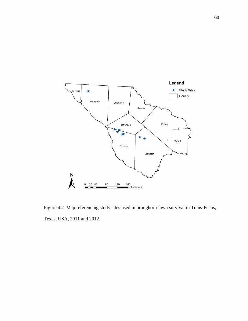
60

Figure 4.2 Map referencing study sites used in pronghorn fawn survival in Trans-Pecos,

Texas, USA, 2011 and 2012.

61

accounts for about 7.3 million hectares. It is bordered to the west and south by the Rio

Grande, to the east by the Pecos River, and to the north by New Mexico (Hatch et al.

1990). Elevation ranges from 762-2,667 meters due to the desert mountain islands

scattered throughout the region. Most precipitation is received during the monsoonal

season between July and October, and annual averages are between 20-30 cm for lower

elevation and 30-46 cm for higher elevations (Simpson et al. 2006).

The study area in Hudspeth County was located in the House and Deep Well

Pastures on the Double U Ranch (University of Texas Lands), 72 km east of El Paso in

north Hudspeth County, Texas (Cannon and Bryant 1997). Hudspeth County is in the

Trans-Pecos mountains and basins ecological area west of the Pecos River. Elevation

ranges from 1,465 m to 1,675 m. Topography ranges from steep to gentle hills on the

west side bordering the Hueco Mountains, to open flats on the east side of the study area

(Cannon and Bryant 1997). This area experiences monsoonal rain, which occurs in late

summer through early fall. The temperature for this region ranges from -18°C in the

winter to over 38°C in the summer (Cannon and Bryant 1997). The study area has

historically been grazed by cattle and still continues today.

The Catto-Gage Ranch in the Marathon Basin is a cattle ranch that is still

operational today. This ranch is located about 29 km east of Alpine, Texas and is 704

km². The portion of this ranch used for the study was mostly the tobosa (Hilaria mutica)

grassland south and adjacent to US Highway 90. The study area was bordered to the west

by the Del Norte Mountains, to the north by US Highway 90 and a neighboring ranch, to

the east by US Highway 385, and to the south by a mesquite (Prosopis glandulosa)-

62

tarbush (Flourensia cernua) scrubland. Climate of the Trans-Pecos was characterized as

arid with an average rainfall of 35.6 cm per year, typically occurring in mid to late

summer (Warnock 1977).

The Marfa Plateau surrounds the town of Marfa, Texas and has historically held

some of the highest densities of pronghorn in the southwestern United States

(Southeastern Cooperative Wildlife Disease Study 1982, O’Gara and Yoakum 2004). The

study area for the Marfa Plateau consisted of 7 ranches scattered across the western

portion of the Marfa Plateau. The ranches were mostly characterized as tobosa (Hilaria

mutica) grasslands, which accounted for as much as 96% of the plant community (Soil

Survey 2013). Two ranches contain tobosa grasslands, but also have rolling igneous hills,

dominated by grama (Bouteloua spp.) and bluestem (Andropogon spp.) grasses along

with forbs such as buckwheat (Erigonum spp.) and crotons (Croton spp.). Elevation

ranges from 1,064 m in the flats to 1,368 m in the hills (USDA 2013). This area is also

characterized by monsoonal rains, where approximately 75% of the precipitation occurs

as thunderstorms of short duration and high intensity during the months of June through

October (USDA 2013). This area receives 28 to 33 cm of rain annually and has

temperatures comparable to those on the Double U Ranch.

METHODS

In order to assess fawn survival and cause of mortality, I captured and radio collared

neonates in 3 different areas throughout the Trans-Pecos. I used the nighttime hoop-net

capture method as described by Brownlee and Hailey (1970) to capture fawns. Fawns

63

were captured shortly after parturition using hoop‐nets, spotlights, and vehicles. A hoop-

net (Tomahawk Live Trap 3350 Mighty Net, Hazelhurst, Wisconsin, USA) was used

when catching pronghorn fawns (Brownlee and Hailey 1970).

During the fawning season, field staff traveled to the study sites and glassed for

pronghorn fawns from vehicles. Once locations of fawns were documented, teams

congregated on the fawning areas using all-terrain vehicles (ATVs) or trucks and

spotlights. After fawns were seen at night, researchers approached fawns on foot and with

ATVs or trucks. Nets were then placed over fawns. Once captured, fawns were

blindfolded to reduce struggling and capture related stress (Byers 1997, Cancino et al.

2005).

An effort was made to minimize capture and handling times to reduce scent

transfer and potential for capture myopathy. Rubber gloves were used by handlers to

decrease the amount of scent transferred to the fawn. A primary assumption of radio-

telemetry studies is that radio-marking does not affect the animals’ behavior, survival, or

reproductive success (Holt et al. 2009). I selected a lightweight, self-adjusting collar used

for young ungulates described by Keister et al. (1988). The study collars weighed 68

grams. Since there is a risk of abandonment, I used cryptic collars (e.g., brown) not

noticeable when attached to a fawn. I attached a collar that was self-adjusting, (ATS

M4210 Expandable Breakaway Collar) lightweight (68 grams), and programmed with a

4-hour mortality sensor, which allowed for recovery of fawns after death.

64

Upon capture I recorded weight, neck circumference, total body length, and new

hoof growth measurement. Ages were estimated using a regression equation:

Y = 0.893549 + 2.3419353 xi

where xi is a new hoof growth measurement for an individual fawn, and Y is the

estimation for age (Tucker 1979, Sams et al. 1996, Flueck and Smith-Flueck 2005)

(Figure 4.3). From these ages, I was able to estimate birthdates for both years (2011,

2012), and I was able to establish length and peak of fawning period in the Trans-Pecos.

Using standard radio-telemetry techniques as described by Barrett (1984) fawns

were monitored each day from the ground to document survival or mortality. If a

mortality signal was detected, the research team would locate the fawn and perform a

thorough and timely investigation to determine cause of death. The immediate area

around the carcass was examined for clues, then the carcass was brought back to a

laboratory for a necropsy. For necropsies, hide was skinned back to examine canine

marks, if present; stomachs were examined to evaluate presence of food; and all other

organs were examined if present. All mortalities were classified and cause of mortality

was recorded for each year.

Fairbanks (1992) found that most pronghorn fawn mortality occurred before the

formation of nursery groups, which was usually around 5-6 weeks after the start of

fawning season. Fawns were monitored for approximately 14 weeks after capture to

determine survival. For the first 60 days post capture, fawns were checked daily. After 60

days of monitoring, ground surveys were reduced to 2x/week.

65

Figure 4.3 New hoof growth was determined by measuring the distance from the hairline

to the ridged growth line (arrow) on the abaxial wall of a front hoof. New hoof growth

and a corresponding regression equation were used to predict pronghorn fawn age during

capture (Tucker 1979, Sams et al 1996, Flueck and Smith-Flueck 2005).

66

Statistical Analysis- All data was first tested for normality using Kolmogorov-Smirnov

test of normality (Zar 2010). The program IBM SPSS Statistics 19 was used for all

statistical analysis except for fawn survival estimates. Since fawn ages differed at time of

capture, I used linear regression analysis to predict fawn weight by age (days) for 2011

and 2012, separately. This standardized all weight and age measurements, which made

comparisons between years possible. The limit for this regression analysis was the

maximum age of a fawn at capture for each year. The Kaplan Meier method in Ecological

Methodology version 7.2 was used to calculate pronghorn fawn survival estimates for

2011 and 2012 (Krebs 1999). For both years, I calculated survival of radio-marked fawns

to 14 weeks using Kaplan-Meier estimator modified for staggered entry (Pollock et al.

1989, White and Garrott 1990, Gregg et al. 2001). To compare survival across years, the

weekly survival estimates were compared using 95% confidence intervals (Zar 2010).

RESULTS

In 2011, fawns were captured from 6 different ranches in 4 areas throughout the Trans-

Pecos (Figures 4.4, 4.5, and 4.6). A total of 26 fawns captured from 4 May 2011–2 June

2011 were fitted with radio-collars. Average weight for fawns captured was 2.4 kg with a

range of 0.95–4.54 kg. Mean neck circumference and total body length was 15.7 cm and

61.5 cm, respectively (Table 4.1).

New hoof growth averaged 4.99 mm. In 2012, fawns were captured from 4

different ranches in 2 different areas in the Marfa Plateau (Figure 4.7). A total of 34

67

Figure 4.4 Pronghorn fawn capture and mortality locations on the Double U Ranch in Hudspeth County, Texas, USA, 2011.

68

Figure 4.5 Pronghorn fawn capture and mortality locations on the Catto-Cage Ranch in Brewster County, Texas, USA, 2011.

69

Figure 4.6 Pronghorn fawn capture and mortality locations in the Marfa Plateau in Jeff Davis and Presidio counties,

Texas, USA, 2011.

70

Table 4.1 Characteristics of pronghorn fawns captured in Trans-Pecos, Texas, USA,

2011-2012.

Averages/Percentages 2011

(n = 26)

2012

(n = 34)

Weight (kg) 2.4 3.8

Age (days) 12.6 9.8

Neck circumference (cm) 15.7 16.7

Body length (cm) 61.5 62.2

Handling time (minutes) 5.9 4.0

Percent twins (%) 53.8 56.0

Dam present (%) 84.6 97.0

71

Figure 4.7 Pronghorn fawn capture and mortality locations in the Marfa Plateau in Jeff Davis and Presidio counties, Texas,

USA, 2012.

72

fawns were captured from 3 May 2012–29 June 2012 and fitted with radio-collars. The

average weight of fawns caught in 2012 was 3.8 kg and ranged from 2.04–6.2 kg. Mean

neck circumference and total body length was 16.6 and 62.2 cm (Table 4.1). New hoof

growth averaged 3.79 mm.

In 2011, average age of fawns at capture was 12.6 days old. The youngest fawn

caught was 3.24 days old, while the oldest fawn was 23.1 days old. Fawning dates were

highly variable resulting in a relatively long fawning period (Figure 4.8). The Hudspeth

County study site appeared to fawn first, followed by the other 3 study sites. In 2012,

average age of fawns at capture was 9.8 days old. The youngest fawn was 3.2 days old

while the oldest fawn was 26.7 days. I documented a fawning period for 2011 and 2012

of 30 and 56 days, respectively (Figure 4.8).

In 2011, of the 26 fawns collared 53.8% were observed as twins at time of

capture, and the dam was present during capture 84.6% of the time. Out of the 34 fawns

caught in 2012, 56% were twins and the dam was present 97% of the time (Table 4.1).

A total of 23 mortalities and 2 surviving fawns was recorded in 2011. Predation

accounted for 96% (n = 22) of the mortalities. One mortality, was unknown (4%), while

one fawn was censored (e.g., transmitter malfunction) and was never located after

capture. Coyote (Canis latrans) and bobcat (Lynx rufus) predation each accounted for

26% (n = 6) of all mortalities in 2011. Another 44% (n = 10) was recorded as unknown

predation. In these cases, the animal had either been dead too long to determine cause of

death or a bloody collar was all that was found. In 2012, 27 mortalities were recorded.

73

Figure 4.8 Estimated pronghorn fawning dates for neonates captured in 2011 and 2012 in

Trans-Pecos, Texas, USA.

74

Bobcat predation was highest of all predators accounting for 37% (10/27) of the

mortalities. Coyote predation was second at 22% (6/27), while unknown predation was

15% (4/27). Other mortality factors totaled 26% (7/27), which included grey fox

(Urocyon cinereoargenreus) and golden eagle (Aguila chrysaetos) predation,

abandonment, and unknown causes (Figure 4.9).

Statistical Analysis-For 2011, weights were estimated using the regression equation:

Y = 0.95 + 0.142 xi

where xi is fawn age in days and Y is the estimation for weight (Zar 2010). For 2012,

weights were estimated using the regression equation:

Y = 2.347 + 0.15 xi

where xi is fawn age in days and Y is the estimation for weight (Zar 2010). Using these

regression equations I was able to standardize weights and ages for both 2011 (R² = 0.53,

P < 0.001) and 2012 (R² = 0.52, P < 0.001), which allowed for better comparison. At 5

days of age, weight in 2011 was approximately 1.64 kg and up to 3.77 kg in 2012. At 20

days of age, weights were estimated to be approximately 3.77 kg and 5.32 kg for 2011

and 2012, respectively (Figure 4.10).

Kaplan Meier survival estimates for both years were found to be similar using

95% confidence intervals. There was almost complete overlap in survival, where 2011

confidence intervals were 0.051 ≤ X̄ ≤ 0.195 and 2012 confidence intervals were 0.075 ≤

X̄ ≤ 0.197. Pronghorn fawn survival in 2011 was 0.027 (SE = 0.03) and in 2012 survival

was 0.044 (SE = 0.03) for a 14 week period (Figure 4.11).

75

Figure 4.9 Mortality factors for pronghorn fawns captured in 2011 and 2012 in Trans-

Pecos, Texas, USA.

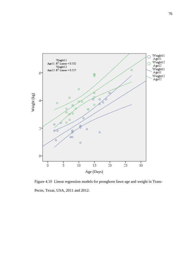
76

Figure 4.10 Linear regression models for pronghorn fawn age and weight in Trans-

Pecos, Texas, USA, 2011 and 2012.

Age (Days)

Wei

ght

(kg)

77

Figure 4.11 Kaplan-Meier survial estimates for captured pronghorn fawns in Trans-

Pecos, Texas, USA, 2011 and 2012.

78

DISCUSSION

Fawn recruitment is essential for pronghorn population growth (Ockenfels 1995). Lee et

al. (1989) proposed that dietary overlap with cattle and sheep, fences that prevent

movement to more suitable habitat, loss of habitat due to human development, water

availability, predators, diseases, and nutritional concerns may play a role in pronghorn

population dynamics. The Trans-Pecos region is experiencing many of these problems

(Sullins 2002, Simpson et al. 2007), which may have contributed to low fawn

recruitment. If populations in arid regions of Texas are limited by forage production,

increases due to rainfall should result in better lactation by females and correspondingly

better nutritional status of fawns and females (Brown et al. 2002).

In 2011, the Trans-Pecos experienced an extreme drought and very low fawn

crops were reported. Twining rates were lower than expected in both 2011 (53.8%) and

2012 (56%). A higher percentage could have been twins, but were not found during

capture or had perished before being caught. Studies throughout the range of pronghorn

indicate that the majority of fawn mortalities are because of predation (Neff and Woolsey

1979, Tucker and Garner 1980, Barrett 1984, Smith et al. 1986, Ockenfels et al. 1992).

During a drought in south Texas, Bradley et al. (2006) recorded that small mammal

populations decreased dramatically as resources (e.g., food and cover) began to diminish,

which is comparable to severe drought conditions in 2011 experienced in the Trans-Pecos

region. It is conceivable that drought may have had an impact on small mammal numbers

in the Trans-Pecos resulting in higher predation rates on pronghorn fawns because of the

lack of alternative prey.

79

I documented high predation on pronghorn fawns both years, but other factors

could have contributed to this high predation. Lactating does on poor nutrition may have

lower milk production and poorer health (Ginnett and Young 2000). In 2011, some fawns

appeared to be severely malnourished with low body weights when compared to 2012.

Condition of dams in late gestation can have a direct effect on birth weight in ungulates

(Thorne et al. 1976). In many cases low birth weight can increase the risk of hypothermia

or starvation (Thorne et al. 1976) or increase chances of predation (Clutton-Brock et al.

1982). Birth weights of pronghorn fawns in some years can affect the survival of fawns

till weaning (Fairbanks 1993).

Birth synchrony can affect predation rates of young for some ungulates (Gregg et

al. 2001). In both 2011 and 2012, I documented very long, extended fawning periods with

only a minor peak in fawning for those 2 years. The lack of precipitation throughout the

winter and spring may have also been an important factor in later fawning dates in 2011.

In 2011 and 2012, the Palmer Drought Severity Index (PDSI) for March through August

and January through May was severely below average (NOAA 2012). A short fawning

period with a distinct peak allows more pronghorn fawns to avoid predation than does a

long fawning period (Gregg et al. 2001). Fawns in the southern part of pronghorn range

generally are born later and over a greater span of time (O’Gara 2004). A study

conducted by Gregg et al. (2001) in Oregon on the northern part of pronghorn range,

documented the birthing pulse to be 12 to 13 days with a peak of 4 to 5 days. Due to this

longer birthing pulse, it took 9 to 11 weeks to see a decline in fawn mortality. Fagan et al.

(2004) recorded a significant positive relationship between winter precipitation and

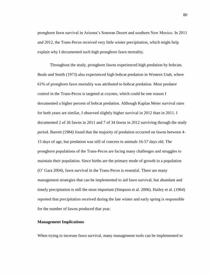
80

pronghorn fawn survival in Arizona’s Sonoran Desert and southern New Mexico. In 2011

and 2012, the Trans-Pecos received very little winter precipitation, which might help

explain why I documented such high pronghorn fawn mortality.

Throughout the study, pronghorn fawns experienced high predation by bobcats.

Beale and Smith (1973) also experienced high bobcat predation in Western Utah, where

61% of pronghorn fawn mortality was attributed to bobcat predation. Most predator

control in the Trans-Pecos is targeted at coyotes, which could be one reason I

documented a higher percent of bobcat predation. Although Kaplan Meier survival rates

for both years are similar, I observed slightly higher survival in 2012 than in 2011. I

documented 2 of 26 fawns in 2011 and 7 of 34 fawns in 2012 surviving through the study

period. Barrett (1984) found that the majority of predation occurred on fawns between 4-

15 days of age, but predation was still of concern to animals 16-57 days old. The

pronghorn populations of the Trans-Pecos are facing many challenges and struggles to

maintain their population. Since births are the primary mode of growth in a population

(O’ Gara 2004), fawn survival in the Trans-Pecos is essential. There are many

management strategies that can be implemented to aid fawn survival, but abundant and

timely precipitation is still the most important (Simpson et al. 2006). Hailey et al. (1964)

reported that precipitation received during the late winter and early spring is responsible

for the number of fawns produced that year.

Management Implications

When trying to increase fawn survival, many management tools can be implemented to

81

aid this process. Proper grazing will ensure fawns have the proper cover needed to hide

from predators. Grazing properly will also decrease the competition with adult

pronghorn, which increases nutrition received by fawns. Also, using predator control

measures during certain times have shown to increase pronghorn fawn survival (Cannon

1995, Spencer and Beach 2006, Brown 2009). Coyotes are the most effective predator at

killing pronghorn fawns (Barrett 1984, Gregg et al. 2001), and most of that mortality

happens before fawns are 1 month old (Barrett 1984). If predators can be reduced from

the landscape prior to the fawning season, fawns should have a better chance of surviving

(Hailey 1979, Neff et al. 1985, Smith et al. 1986). Hailey (1979) and Neff et al. (1985)

found that fawn crops significantly increased when predator control was implemented

from November through January. Fences and barriers to movements can be detrimental to

pronghorn populations including fawns (Hailey et al. 1966). Removing these barriers will

allow pronghorn to move to areas of better nutrition benefitting both adults and their

fawns (Gray 2012). Range conditions and pronghorn nutrition are yet to be evaluated in

the Trans-Pecos. If adult female pronghorn are not getting adequate nutrition needed to

raise fawns then the rest of these factors are secondary. Also, it would be beneficial to

study birth synchrony, and how that affects predation on neonatal fawns. Birth synchrony

is a very important prey defense mechanism (Dauphine and McClure 1974) that may be

affected by drought and other unknown factors.

LITERATURE CITED

Barrett, M. W. 1984. Movements, habitat use, and predation on pronghorn fawns in

Alberta. Journal of Wildlife Management 48:542-550.

82

Beale, D. M., and A. D. Smith. 1973. Mortality of pronghorn antelope fawns in western

Utah. Journal of Wildlife Management 37:343–352.

Bradley R. D., J. D. Hanson, B. R. Amman, B. D. Baxter, D. S. Carroll, N. D. Durish, M.

L. Haynie, M. Kageyama, L. K. Longhofer, F. M. Mendez-Harclerode, S. A.

Reeder, J. R. Suchecki, D. C. Ruthven, III, M. N. B. Cajimat, C. Milazzo, Jr., M.

L. Milazzo, and C. F. Fulhorst. 2006. Rapid recovery of rodent populations

following severe drought. Southwestern Naturalist 51:87-93.

Brown, D. E., W. F. Fagan, R. Lee, H. G. Shaw, and R. B. Turner. 2002, "Winter

precipitation and pronghorn fawn survival in the Southwest." In Proceedings of

the Biennial Pronghorn Workshop, Kearney, Nebraska 20:115-122.

Brown, D. E. 2009. Effects of coyote removal on pronghorn and mule deer populations in

Wyoming. Thesis, Utah State University, Logan, USA.

Brownlee, S., and T. L. Hailey. 1970. Development of a technique for night trapping

antelope fawns. Proceedings from the Pronghorn Workshop 4:78-81.

Byers, J. A. 1997. Mortality risk to young pronghorns from handling. Journal of

Mammalogy 79:1416–1431.

Cancino, J., V. S. Sotomayor, and R. Castellanos. 2005. From the field: Capture, hand-

raising, and captive management of peninsular pronghorn. Wildlife Society

Bulletin 33:61–65.

Canon, S. K. 1995. Management of coyotes for pronghorn? Pages 97-103 in D. Rollins,

C. Rich-ardson, T. Blankenship, K. Canon, and S. E. Henke, editors. Coyotes in

83

the Southwest: a compendium of our knowledge. Texas Parks & Wildlife

Department, Austin, Texas, USA.

Canon, S. K., and F. C. Bryant. 1997. Bed-site characteristics of pronghorn fawns.

Journal of Wildlife Management 61:1134-1141.

Clutton-Brock, T. H., F. E. Guinness, and S. D. Albon. 1982. Red deer: Behavior and

ecology of two sexes. University of Chicago Press, Chicago, Illinois, USA.

Dauphine, T. C., Jr., and R. L. McClure. 1974. Synchronous mating in Canadian barren-

ground caribou. Journal of Wildlife Management 38:54-66.

Edwards, W. C. 1958. A study of the reproductive potential and ovarian structures in the

pronghorn antelope, Antilocapra americana (Ord) in Wyoming. Thesis,

University of Wyoming, Laramie, USA.

Fagan, W. F., D. E. Brown, R. Lee, H. G. Shaw, and B. Turner. 2004. Winter

precipitation and pronghorn fawn survival in the southwest. Proceedings of the

Pronghorn Antelope Workshop. Bismarck, North Dakota, USA.

Fairbanks, W. S. 1992. Dominance, aggression, and reproductive success in female

pronghorn. Dissertation, University of Kansas, Lawrence, USA.

Flueck, W. T., and J. M. Smith-Flueck. 2005. Hoof growth in neonatal Patagonian

huemul (Hippocamelus bisulcus): A tentative tool for aging. Mastozoologia

Neotropical 12:245-248.

Ginnett, T. F., and E. L. B. Young. 2000. Stochastic recruitment in white-tailed deer

along an environmental gradient. Journal of Wildlife Management 64:713–720.

84

Gray, S. S. 2012. Big game research and surveys: Pronghorn harvest recommendations.

Federal Aid Project W-127-R-20. Texas Parks and Wildlife Department.

Gregg, M. A., M. Bray, K. M. Kilbride, and M. R. Dunbar. 2001. Birth synchrony and

survival of pronghorn fawns. Journal of Wildlife Management 65:19-24.

Hailey, T. L., D. Dearment, and P. Evans. 1964. Pronghorn decline. Texas Game and

Fish 22:22-23.

Hailey, T. L., J. W. Thomas, and R. M. Robinson. 1966. Pronghorn die-off in Trans-

Pecos Texas. The Journal of Wildlife Management 30:488-496.

Hailey, T. L. 1979. A handbook for pronghorn antelope management in Texas. Series

20, Texas Parks and Wildlife Department, Austin, Texas.

Hatch, S. L., Gandhi, K. N., and Brown, L. E. 1990. Checklist of the vascular plants of

Texas. College Station, Texas: Texas Agricultural Experiment Station iv, 158p.

Maps Plant records. Geography, 3.

Hepworth, W. G., and F. Blunt. 1966. Research findings on Wyoming antelope.

Wyoming Wildlife 30:24-29.

Holt, R. D., L. W. Burger, Jr., S. J. Dinsmore, M. D. Smith, S. J. Szukaitis, and K. D.

Godwin. 2008. Estimating duration of short-term acute effects of capture

handling and radiomarking. Journal of Wildlife Management 73:989–995.

Keister, G. P., Jr., C. E. Trainer, and M. J. Willis. 1988. A self-adjusting collar for

young ungulates. Wildlife Society Bulletin 16:321–323.

Krebs, C. J. 1999. Ecological methodology. Second edition. Addison Wesley Longman,

Menlo, California, USA.

85

Lee, T. L., J. Derr, J. Bickham, and T. Clark. 1989. Genetic variation in pronghorn from

west Texas. Journal of Wildlife Management 53:890-896.

Neff, D. J., and N. G. Woolsey. 1979. Effect of predation by coyotes on antelope fawn

survival on Anderson Mesa. Report 8. Arizona Game and Fish Department,

Phoenix Special.

Neff, D. J., R. H. Smith, and N. W. Woolsey. 1985. Pronghorn antelope mortality study.

Arizona Game and Fish Department Final Report, Fed. Aid Project. W-78- R;

WP2, J16.

National Oceanic and Atmospheric Administration (NOAA). The Palmer drought

severity index, <ftp://ftp.ncdc.noaa.gov/pub/data/cirs/drd964x.pdsi.txt> (October,

2012).

Ockenfels, R. A., C. L. Dorothy, and J. D. Kirkland. 1992. Mortality and home range

of pronghorn fawns in central Arizona. Proceedings of the Pronghorn Antelope

Workshop 15:78–92.

Ockenfels, R. A. 1995. Pronghorn in the Southwest. Pages 12-15 in B. Kattnig and M.

Scheider, editors. Predator-prey population dynamics workshop. United States

Department of Agriculture Cooperative Extension Service, University of Arizona

and New Mexico State University, Tucson, Arizona, USA.

O’Gara, B. W. 1968. A study of the reproductive cycle of the female pronghorn

(Antilocapra americana Ord). Dissertation, University of Montana, Missoula,

USA.

86

O’Gara, B. W. 2004. Reproduction. Pages 275-298 in B. W. O’ Gara, and J. D. Yoakum,

editors. Pronghorn: Ecology and management. University Press of Colorado,

Boulder, Colorado, USA.

O’ Gara, B. W., and J. D. Yoakum. 2004. Pronghorn: Ecology and management.

University Press of Colorado, Boulder, Colorado, USA.

Pollock, K. H., S. R. Winterstein, C. M. Bunck, and P. D. Curtis. 1989. Survival analysis

in telemetry studies: The staggered entry design. Journal of Wildlife

Management 53:7-15.

Sams, M. G., R. L. Lochmiller, E. C. Hellgren, W. D. Warde, and L. W. Varner. 1996.

Morphometric predictors of neonatal age for white-tailed deer. Wildlife Society

Bulletin 24:53-57

Simpson, D. C., L. A. Harveson, C. E. Brewer, R. E. Walser, and A. R. Sides. 2006.

Influence of precipitation on pronghorn demography in Texas. Journal of Wildlife

Management 71:906-910.

Smith, R. H., D. J. Neff, and N. G. Woolsey. 1986. Pronghorn response to coyote

control: A benefit:cost analysis. Wildlife Society Bulletin 14:226-231.

Soil Survey Staff, Natural Resources Conservation Service [NRCS] United States

Department of Agriculture [USDA]. Web Soil Survey.

<http://websoilsurvey.nrcs.usda. gov/>. Accessed 10 Jan 2013.

Southeastern Cooperative Wildlife Disease Study Team. 1982. Densities of pronghorn

antelope where suitable habitat exists. University of Georgia School Veterinarian

Science, Athens, USA.

87

Spencer, J. O., Jr., and Beach, R. H. 2006. Wildlife damage management protection

efforts for a vulnerable pronghorn antelope population in northwestern Nevada:

2000-2004. Proceedings from the Vertebrae Pest Conference 22:269-273.

Sullins, M. R. 2002. Factors affecting pronghorn antelope populations in Trans-Pecos,

Texas. Pages 29-36 in L. A. Harveson, C. Richardson, and P. M. Harveson,

editors. Proceedings of the Trans-Pecos Wildlife Conference. Sul Ross State

University, 1-2 August 2002, Alpine, Texas, USA.

Thorne, E. T., R. E. Dean, and W. G. Hepworth. 1976. Nutrition during gestation in

relation to successful reproduction in elk. Journal of Wildlife Management

40:330-335.

Tucker, R. D. 1979. Pronghorn antelope fawn mortality, home range habitat, and

behavior in Brewster County, Texas. Thesis, Sul Ross State University, Alpine,

Texas, USA.

Tucker, R. D., and G. W. Garner. 1980. Mortality of pronghorn antelope fawns in

Brewster County, Texas. Proceedings of the Western Association of Fish and

Wildlife Agencies 60: 620-631.

United States Department of Agriculture [USDA]. <www.usda.gov>. Accessed 21 Jan

2013.

Warnock, B. H. 1977. Wildflowers of the Davis Mountains and the Marathon Basin,

Texas. Thesis, Sul Ross State University, Alpine, Texas, USA.

White, G. C., and R. A. Garrott. 1990. Analysis of wildlife radio-tracking data.

Academic Press, San Diego, California, USA.

88

Zar, J. H. 2010. Biostatistical analysis. 5th

Edition. Pearson Prentice Hall, Upper Saddle

River, New Jersey, USA.

89

Appendix A. Horn measurements, cementum annuli age estimations, and kidney fat

indices collected from harvested pronghorn bucks in Trans-Pecos, Texas, 2010-2011.

a Year-

Sample ID #

Beam Length

(cm)

Base

(cm)

Prong Length

(cm)

Inside Spread

(cm)

Age

(Yrs)

Kidney

Fat Index

(%)

10-001 30.80 11.75 9.84 28.26 7 12.3

10-004 37.78 15.24 11.11 48.26 5 52.3

10-006 30.16 23.81 7.30 21.91 5 7.6

10-007 30.16 13.02 7.94 22.54 7 10.4

10-010 34.93 13.97 8.89 29.85 3 12.5

10-012 24.13 14.61 6.35 24.77 - -

10-015 41.59 15.88 13.97 23.81 - 7.6

10-017 35.24 14.61 12.70 31.12 5 16.9

10-021 35.88 17.15 12.07 28.89 4 27.7

10-022 41.59 15.24 11.75 37.47 4 9.7

10-027 30.16 13.97 10.16 24.13 4 9.5

10-030 33.97 13.02 10.48 27.31 6 10.7

10-035 33.34 23.18 11.75 38.42 6 5.2

10-037 27.94 12.70 9.53 29.85 3 -

10-038 39.37 14.92 13.34 29.85 5 1.8

10-039 33.34 12.70 6.03 17.78 4 11.1

10-041 33.02 13.65 12.07 26.67 6 11.5

10-042 37.47 15.24 16.51 32.07 6 2.2

10-049 35.24 14.92 8.89 27.94 5 9.6

a 10 refers to 2010, 11 refers to 2011

90

a Year-

Sample ID #

Beam Length

(cm)

Base

(cm)

Prong Length

(cm)

Inside Spread

(cm)

Age

(Yrs)

Kidney

Fat Index

(%)

10-051 34.29 12.70 10.80 36.20 4 1.8

10-054 36.83 15.24 12.38 28.26 5 10.8

10-058 30.48 14.29 11.11 22.86 3 22.3

10-061 - - - - 4 14.8

10-062 - - - - 4 0.3

10-063 32.70 15.24 11.43 30.48 5 10.6

10-064 33.66 15.56 14.61 25.72 6 11.1

10-066 35.56 15.24 10.16 20.96 5 0.3

10-068 38.74 14.92 10.48 N/A 4 16.5

10-069 39.05 15.56 10.80 30.48 3 1.9

10-070 31.43 17.15 10.16 33.02 7 13.2

10-080 37.47 13.97 12.70 27.94 7 14.7

10-082 35.88 16.51 11.43 22.54 5 18.6

10-083 16.51 7.62 N/A 30.48 - 4.2

10-084 32.70 13.02 12.38 25.40 4 6.2

10-086 36.83 15.24 9.84 19.05 5 21.5

10-089 33.97 16.19 9.21 25.08 5 15.3

10-090 34.61 15.56 15.24 23.50 7 21.6

10-092 - - - - - 8.5

10-093 31.12 15.88 11.11 25.40 6 7.1

10-095 34.61 15.24 13.34 29.53 4 5.7

10-105 36.83 13.97 12.07 27.94 4 21.3

91

a Year-

Sample ID #

Beam Length

(cm)

Base

(cm)

Prong Length

(cm)

Inside Spread

(cm)

Age

(Yrs)

Kidney

Fat Index

(%)

10-106 31.12 14.61 13.97 25.72 5 15

10-107 27.31 13.65 9.84 24.77 6 32.2

10-108 30.16 13.34 11.43 24.77 3 15.2

10-109 34.29 14.92 10.48 27.62 4 1.2

10-111 34.29 13.97 11.43 11.75 3 12

10-112 - - - - 6 9.7

10-114 37.47 13.02 13.02 25.72 4 11.1

10-117 35.24 13.97 10.16 34.61 9 0.4

10-118 31.43 13.65 8.89 24.77 5 3.8

10-119 30.48 13.65 7.30 21.27 5 17.3

10-122 31.43 13.97 12.70 36.83 11 8.5

10-125 34.29 16.51 11.43 26.67 5 1.7

10-127 33.34 14.29 11.43 25.40 5 38.6

10-132 - - - - 8 20.8

10-138 34.29 12.07 10.80 25.40 5 10.8

10-139 30.16 13.34 8.57 22.54 3 78.2

10-146 41.91 14.92 12.70 34.93 6 2.2

10-147 34.61 13.34 10.16 32.39 2 2

10-152 36.20 14.29 9.84 22.86 7 9.9

10-153 37.78 13.97 12.38 19.69 5 20.9

10-157 34.61 13.97 13.02 18.42 5 5.5

10-159 34.29 14.92 10.80 29.21 5 15.2

92

a Year-

Sample ID #

Beam Length

(cm)

Base

(cm)

Prong Length

(cm)

Inside Spread

(cm)

Age

(Yrs)

Kidney

Fat Index

(%)

10-160 29.85 13.97 11.11 19.37 5 46.8

10-162 35.56 13.97 8.26 30.48 7 20.9

10-164 35.56 14.61 9.21 27.31 5 9

10-165 31.43 16.83 11.43 29.85 5 27

10-167 34.93 16.19 13.34 31.43 13 19.6

10-170 34.61 14.61 11.75 18.42 11 41.7

10-171 - - - - 6 13.7

10-172 35.56 15.24 10.16 14.29 5 10.6

10-173 35.24 13.65 10.16 17.15 5 41.3

10-174 33.02 14.61 9.84 25.08 6 25

10-176 35.88 16.51 13.02 31.12 5 3.2

10-178 34.61 16.19 10.48 26.35 8 2.6

10-179 35.56 13.97 10.48 26.04 5 9.1

10-183 33.02 13.34 9.53 31.75 5 17.3

10-184 13.34 7.94 15.24 33.66 4 13.23

10-186 31.12 13.97 9.53 28.89 6 10.3

10-187 39.37 15.88 11.11 30.80 5 4.8

10-188 36.51 14.61 11.11 34.61 7 13.4

10-189 32.70 12.70 6.35 25.40 4 0.3

10-195 30.48 10.80 7.62 18.10 4 22.7

10-196 - - - - - 0.5

10-199 37.47 15.24 12.07 22.23 5 10.9

93

a Year-

Sample ID #

Beam Length

(cm)

Base

(cm)

Prong Length

(cm)

Inside Spread

(cm)

Age

(Yrs)

Kidney

Fat Index

(%)

10-201 40.01 15.88 13.34 28.26 3 11.7

10-202 40.01 18.42 15.24 N/A 6 3

10-204 - - - - 5 0.7

11-001 14.75 5.38 2.75 8.38 6 27.3

11-006 13.75 5.63 3.38 11.00 7 0.7

11-007 13.50 5.38 4.75 9.00 - 7.6

11-008 12.63 5.50 4.13 8.50 6 10.8

11-009 12.88 6.13 3.63 16.00 6 12.4

11-010 12.88 6.00 3.75 11.00 4 12

11-011 13.88 5.38 4.38 7.63 6 18.2

11-012 12.50 5.88 5.00 9.13 6 5.7

11-014 13.25 5.63 4.88 11.88 7 19.3

11-017 11.50 5.88 5.50 9.50 6 3.8

11-020 12.00 5.25 4.50 12.50 6 4.3

11-021 13.25 5.75 5.00 11.00 5 5.4

11-029 12.63 5.38 4.50 7.25 6 5.5

11-031 15.88 6.13 6.25 12.00 4 6.8

11-034 13.00 5.50 4.00 9.38 4 16.1

11-036 11.88 5.75 3.50 9.25 7 4.1

11-037 13.25 5.88 4.00 8.13 11 1.8

11-039 16.00 6.13 6.25 10.00 3 -

11-040 15.25 6.00 5.25 10.00 3 2.6

94

a Year-

Sample ID #

Beam Length

(cm)

Base

(cm)

Prong Length

(cm)

Inside Spread

(cm)

Age

(Yrs)

Kidney

Fat Index

(%)

11-041 14.25 5.50 4.50 13.00 N/A 5.7

11-044 13.00 5.88 3.50 12.13 3 11.9

11-045 - - - - 2 18.5

11-046 - - - - - -

11-049 16.25 6.38 5.50 10.25 5 6.9

11-050 11.00 5.25 2.25 9.63 9 7.6

11-051 14.75 5.88 4.25 10.25 3 16.5

11-052 15.25 6.25 5.25 9.75 4 7.9

11-053 13.25 6.13 5.00 9.00 5 12.5

11-056 15.00 6.25 5.25 10.00 4 0.7

11-058 - - - - - 5.6

11-059 12.00 4.50 2.50 8.75 5 8

11-060 13.25 4.33 3.50 8.25 - 5

11-061 - - - - - 12.3

11-068 15.50 6.25 5.38 9.00 4 7.9

11-069 - - - - 3 -

11-070 14.75 4.75 3.00 9.75 6 6.8

11-073 14.00 5.75 4.50 10.00 4 2

11-074 - - - - 4 -

11-079 16.00 6.00 3.75 - 6 1.3

11-081 15.88 6.50 5.00 17.25 2 10.1

11-082 13.13 5.38 4.13 7.25 6 0

95

a Year-

Sample ID #

Beam Length

(cm)

Base

(cm)

Prong Length

(cm)

Inside Spread

(cm)

Age

(Yrs)

Kidney

Fat Index

(%)

11-090 - - - - - 10

96

VITA

James H Weaver

P.O. Box 1732,

Fort Davis, Texas, 79734

903-335-0947

jamesweaver04@gmail.com

Education:

M.S., Range and Wildlife Management, Sul Ross State University, 2013

B.S., Wildlife and Conservation Science, Texas A&M University-Commerce, 2010

Experience:

Wildlife Technician, Texas Parks and Wildlife Department, Alpine, Texas

Graduate Research Assistant, Borderlands Research Institute for Natural Resource

Management, Sul Ross State University, Alpine, Texas

Volunteer Research Assistant, Department of Natural Resource Management, Sul Ross

State University, Alpine, Texas

Volunteer Research Assistant, College of Forestry and Conservation, University of

Montana, Missoula, Montana

Volunteer Field Technician, Texas Parks and Wildlife Department, Sulphur Springs,

Texas