The role of modeling in systems biology - DBK...

Chapter 1

The role of modeling in

systems biology

Douglas B. Kell & Joshua D. Knowles

The use of models in biology is at once both familiar and arcane. It is

familiar because, as we shall argue, biologists presently and regularly use models

as abstractions of reality: diagrams, laws, graphs, plots, relationships, chemical

formulae and so on are all essentially models of some external reality that we

are trying to describe and understand (Fig. 1.1). In the same way we use and

speak of ‘model organisms’ such as baker’s yeast or Arabidopsis thaliana, whose

role lies in being similar to many organisms without being the same as any

other one. Indeed, our theories and hypotheses about biological objects and

systems are in one sense also just models. Yet the use of models is for most

biologists arcane because familiarity with a subset of model types, especially

quantitative mathematical models, has lain outside the mainstream during the

last 50 years of the purposely reductionist and qualitative era of molecular

biology. It is largely these types of model that are an integral part of the ‘new’

(and not-so-new) Systems Biology and on which much of the rest of this book

concentrates. Since all such models are developed for some kind of a purpose,

our role in part is to explain why this type of mathematical model is both useful

and important, and will likely become part of the standard armory of successful

biologists.

1

CHAPTER 1. THE ROLE OF MODELING IN SYSTEMS BIOLOGY 2

Figure 1.1: Models in biology. Although we shall be concentrating here on a

subset of mathematical models, we would stress that the use of all sorts of models

is entirely commonplace in biology – examples include (a) diagrams (here a

sequence of bases and the ‘central dogma’), (b) laws (the flux-control summation

theorem of Metabolic Control Analysis), (c) graphs – in the mathematical sense

of elements with nodes and edges (a biochemical pathway), (d) plots (covariation

of 2 metabolites in a series of experiments), (e) relationships (a rule describing

the use of the concentration of a metabolite in disease diagnosis), (f) chemical

formulae (tryptophan), (g) images (of mammalian cells), etc.


1.1 Philosophical overview

“When one admits that nothing is certain one must, I think, also

admit that some things are much more nearly certain than others.”

Bertrand Russell, ”Am I an Atheist or an Agnostic?”, 1947

It is conventional to discriminate (as in Fig. 1.2) (a) the world of ideas,

thoughts or other mental constructs and (b) the world of observations or data,

and most scientists would recognize that they are linked in an iterative cycle, as

drawn: we improve our mental picture of the world by carrying out experiments

that produce data, and such data are used to inform the cogitations that feed

into the next part of the right-hand arc, that designs and performs the next set

of experiments as part of an experimental program. Such a cycle may be seen

as a ‘chicken and egg’ cycle, but for any individual turn of the cycle there is a

clear distinction between the two essential starting points (ideas or data). This

also occurs in scientific funding circles – is the activity in question ideas- (i.e.

hypothesis-) driven or is it data-driven? (Until recently, the latter, hypothesis-

generating approach was usually treated rather scornfully.)

Figure 1.2: The iterative relationship between the world of

ideas/hypotheses/thoughts and the world of data/observations. Note that

these are linked in a cycle, in which one arc is not simply the reverse of the

other (Kell, 2002; Kell, 2005; Kell & Welch, 1991).

From a philosophical point of view, then, the hypothetico-deductive analy-

sis, in which an idea is the starting point (however muddled or wrongheaded


that idea may be), has been seen as much more secure, since deductive reason-

ing is sound in the sense that if an axiom is true (as it is supposed to be by

definition) and the observation is true, we can conclude that the ‘facts’ are at

least consistent with the idea. If the hypothesis is ‘all swans are white’ then the

prediction is that a measurement of the whiteness of known swans will give a

positive response. By contrast, it has been known since the time of Hume that

inductive reasoning, by which we seek to generalize from examples (“swan A

is white, swan B is white, swan C is white . . . so I predict that all swans are

white”) is insecure – and a single black swan shows it. Nothing will ever change

that, and the ‘problem of induction’ probably lies at the heart of Popper’s insis-

tence (see (Popper, 1992) and/or more readable commentators such as Medawar

(Medawar, 1982)) that theories can only be disproved. Note of course that it is

equally true for the hypothetico-deductive mode of reasoning that a single black

swan will disprove the hypothesis. This said, the ability of scientists to ignore

any number of ugly facts that would otherwise slay a beautiful hypothesis is

well known (Gilbert & Mulkay, 1984), and in this sense – given that there are

no genuinely secure axioms (Hofstadter, 1979; Nagel & Newman, 2002) – the

deductive mode of reasoning is not truly much more secure than is induction.

Happily, there is emerging a more balanced view of the world. This

recognizes that for working scientists the reductionist and ostensibly solely

hypothesis-driven agenda has not been as fruitful as had been expected. In

large measure in biology this realization has been driven by the recognition, fol-

lowing the systematic genome sequencing programs, that the existence, let alone

the function, of many or most genes – even in well-worked model organisms –

had not been recorded. This could be seen in part as a failure of the reductionist

agenda. In addition there are many areas of scientific activity that have nothing

to do with testing hypotheses but which are exceptionally important (Kell &

Oliver, 2004); perhaps chief among these is the development of novel methods.

In particular there are fields – functional genomics not least among them (Kell

& King, 2000), although this is very true for many areas of medicine as well

– that are data-rich but hypothesis-poor, and are best attacked using methods

that are data-driven and thus essentially inductive (Kell & King, 2000).

A second feature that has emerged from a Popperian view of the world (or at

least from his attempt to find a means that would allow one to discriminate ‘sci-

ence’ from ‘pseudo-science’ (Medawar, 1982; Popper, 1992)) is the intellectual


significance of prediction: if your hypothesis makes an experimentally testable

(and thus falsifiable) prediction it counts as ‘science’, and if the experimental

prediction is consistent with the prediction then (confidence in) the ‘correctness’

of your hypothesis or world-view is bolstered (see also (Lipton, 2005)).

1.2 Historical context

The history of science demonstrates that both inductive and deductive reasoning

occur at different stages in the development of ideas. In some cases, such as in

the history of chemistry, a period of almost purely inductive reasoning (stamp-

collecting and classification) is followed by the development of more powerful

theories that seek to explain and predict many phenomena from more general

principles. Often these theories are reductionist, that is to say, complicated

phenomena that seem to elude coherent explanation are understood by some

form of breaking down into constituent parts, the consideration of which yields

the required explanation of the more complicated system. A prime example

of the reductionist mode is the explanation of the macroscopic properties of

solids, liquids and gases – such as their temperature, pressure and heat – by

considering the average effect of a large number of microscopic interactions be-

tween particles, governed by Newtonian mechanics. For the first time, accurate,

quantitative predictions with accompanying, plausible explanations were possi-

ble, and unified much of our basic understanding of the physical properties of

matter.

The success of early reductionist models in physics, and later those in chem-

istry, led in 1847 to a program to analyze (biological) processes, such as urine

secretion or nerve conduction, in physico-chemical terms proposed by Ludwig,

Helmholtz, Brucke and du Bois-Reymond (Bynum et al., 1981). However, al-

though reductionism has been successful in large part in the development of

physics and chemistry, and to a great extent in acquiring the parts list for

modern biology – consider the gene – the properties of many systems resist

a reductionist explanation (Sole & Goodwin, 2000). This ultimate failure of

reductionism in biology, as in other disciplines, is due to a number of factors,

principal among them being the fact that biological systems are inherently com-

plex.

Although complexity is a phenomenon about which little agreement has been


reached, and certainly for which no all-encompassing measure has been estab-

lished, the concept is understood to pertain to systems of interacting parts.

Having many parts is not necessary: it is sufficient that they are coupled in

some way, so that the state of one of them affects the state of one or more

others. Often the interactions are non-linear so, unlike systems which can be

modeled by considering averaged effects, it is not possible to reduce the system’s

behavior to the sum of its parts (Davey & Kell, 1996). Common interactions in

these systems are feedback loops, in which, as the name suggests, information

from the output of a system transformation is sent back to the input of the

system. If the new input facilitates and accelerates the transformation in the

same direction as the preceding output, they are positive feedback - their effects

are cumulative. If the new data produce an output in the opposite direction

to previous outputs, they are negative feedback — their effects stabilize the

system. In the first case there is exponential growth or decline; in the second

there is maintenance of the equilibrium. These loops have been studied in a

variety of fields, including control engineering, cybernetics and economics. An

understanding of them and their effects is central to building and understanding

models of complex systems (Kell, 2004; Kell, 2005; Milo et al., 2002).

Negative feedback loops are typically responsible for regulation and they are

obviously central to homeostasis in biological systems. In control engineering,

such systems are conveniently described using Laplace transforms — a means

of simplifying the combination and manipulation of ODEs, and closely related

to the Fourier transform (Ogata, 2001); Laplace transforms for a large variety

of different standard feedback loops are known and well-understood, though

analysis and understanding of non-linear feedback remains difficult (see Chap-

ter ch11 for details). Classical negative feedback loops are considered to pro-

vide stability (as indeed they do when in simple systems in which the feedback is

fast and effective), though we note that negative feedback systems incorporating

delays can generate oscillations (e.g. (Nelson et al., 2004)).

Positive feedback is a rather less appreciated concept for most people and,

until recently, it could be all but passed over in even a control engineer’s edu-

cation. This is perhaps because it is often equated with undesired instability in

a system, so it is just seen as a nuisance; something which should be reduced

as much as possible. However, positive feedback should not really be viewed in

this way, particularly from a modeling perspective, because it is an important


factor in the dynamics of many complex systems and does lead to very familiar

behavior. One very simple model system of positive feedback is the Polya urn

(Arthur, 1963; Barabasi & Albert, 1999; Johnson & Kotz, 1977). In this, one

begins with a large urn containing two balls, one red and one black. One of

these is removed. It is then replaced in the urn, together with another ball of

the same color. This process is repeated until the urn is filled up. The system

exhibits a number of important characteristics with respect to the distribution

of the two colors of balls in the full urn. In particular: early, essentially ran-

dom events can have a very large effect on the outcome; there is a lock-in effect

where later in the process, it becomes increasingly unlikely that the path of

choices will shift from one to another (notice that this is in contrast to the

“positive feedback causes instability” view); and accidental events early on do

not cancel each other out. The Polya urn is a model for such things as genetic

drift in evolution, preferential attachment in explaining the growth of scale-free

networks (Barabasi & Albert, 1999), and the phenomenon whereby one of a

variety of competing technologies (all but) takes over in a market where there

is a tendency for purchasers to prefer the leading technology, despite equal, or

even inferior, quality compared with the others (e.g. QWERTY keyboards, and

Betamax versus VHS video). (See also (Goldberg, 2002; Kauffman et al., 2000)

for the adoption of technologies as an evolutionary process.)

Positive feedback in a resource-limited environment also leads to familiar

behavior. The fluctuations seen in stock prices, the variety of sizes of sandpiles,

and cycles of population growth and collapse in food-chains all result from this

kind of feedback. There is a tendency to reinforce the growth of a variable

until it reaches a value that cannot be sustained. This leads to a crash which

‘corrects’ the value again, making way for another rise. Such cyclic behavior

can be predictably periodic but in many cases the period of the cycle is chaotic

– i.e. deterministic but essentially unpredictable. All chaotic systems involve

non-linearity, and this is most frequently the result of some form of positive

feedback, usually mixed with negative feedback (Glendinning, 1994; Tufillaro

et al., 1992; Strogatz, 2000). Behavior involving oscillatory patterns may also be

important in biological signaling (Lahav et al., 2004; Nelson et al., 2004), where

the downstream detection may be in the frequency rather than the amplitude

(i.e. simply concentration) domain (Kell, 2005).

All of this said, despite encouraging progress (e.g. (Tyson et al., 2003;


Wolf & Arkin, 2003; Yeger-Lotem et al., 2004)), we are far from having a full

understanding of the behavior of concatenations of these simple motifs and

loops. Thus, the Elowitz and Leibler oscillator (Elowitz & Leibler, 2000) is

based solely on negative feedback loops but is unstable. However, this system

could be made comparative stable and robust by incorporating positive feedback

loops, which led to some interesting work by Ferrell on the cell cycle (Angeli

et al., 2004; Pomerening et al., 2003).

It is now believed that most systems involving interacting elements have both

chaotic and stable regions or phases, with islands of chaos existing within stable

regions, and vice versa (for a biological example, see (Davey & Kell, 1996)).

Chaotic behavior has now been observed even in the archetypal, clockwork sys-

tem of planetary motion; whereas the eye at the heart of a storm is an example

of stability occurring within a wildly unpredictable whole.

Closely related to the vocabulary of complexity and of chaos theory is the

slippery new (or not so new?) concept of emergence (Davies, 2004; Holland,

1998; Johnson, 2001; Kauffman, 2000; Morowitz, 2002). Emergence is generally

taken to mean simply that the whole is more than (and maybe qualitatively

different from) the sum of its parts, or that system-level characteristics are not

easily derivable from the ‘local’ properties of their constituents. The label of

emergent phenomenon is being applied more and more in biological processes at

many different levels, from how proteins can fold to how whole ecosystems evolve

over time. A central question that the use of the term “emergence” forces us to

consider is whether it is only a convenient way of saying that the behavior of

the whole system is difficult to understand in terms of basic laws and the initial

conditions of the system elements (weak emergence), or whether, in contrast,

the whole cannot be understood by the analysis of the parts, and current laws of

physics, even in principle (strong emergence). The latter view would imply that

high level phenomena are not reducible to physical laws (but may be consistent

with them) (Davies, 2004). If this were true, then the modeling of (at least)

some biological processes should not follow solely a bottom-up approach, hoping

to go from simple laws to the desired phenomenon, but might eventually need

us to posit high-level organizing principles and even downward causality. Such

a world view is completely antithetical to materialism and remains as yet on

the fringes of scientific thought.

In summary, reductionism has been highly successful in explaining some


macroscopic phenomena, purely in terms of the behavior of constituent parts.

However, this was predicated (implicitly) on the assumption that there were few

parts (e.g. the planets) and that their interactions were simple, or that there

were many parts but their interactions could be neglected (e.g. molecules in a

gas). However, the scope of a reductionist approach is limited because these

assumptions are not true in many systems of interest (Kell & Welch, 1991; Sole

& Goodwin, 2000). The advent of computers and computer simulations led

to the insight that even relatively small systems of interacting parts (e.g. the

Lorenz model) could exhibit very complex (even chaotic) behavior. Although

the behavior may be deterministic, complex systems are hard to analyze us-

ing traditional mathematical and analytical methods. Prediction, control and

understanding arise mainly from modeling these systems using iterated com-

puter simulations. Biological systems, which are inherently complex, must be

modeled and studied in this way if we are to continue to make strides in our

understanding of these phenomena.

Some phenomena cannot be explained by averaged effects because of the

presence of unstable or quasi-stable attractors that ‘emerge’ as the result of

many non-linear interactions. Turbulence, weather systems, stock prices, the

population sizes of organisms in a food-chain, and sand pile volumes are now

classic examples of systems that are deemed ‘complex’ and which are explained

today by ‘emergence’. The exact initial conditions of some such systems can

influence the long term behavior in ways that are entirely deterministic – but

which are nevertheless impossible to determine in practice because of the impos-

sibility of obtaining sufficiently precise measurements. Modeling these systems

can, however, reveal such things as the boundaries of the regions of stability

within which the accurate, long-term evolution of the system can be predicted,

the conditions under which the system will become chaotic or enter oscillations

– and even many useful parameters governing the limits of the chaotic behavior,

albeit predicting tomorrow’s gold price remains elusive. In biology, very many

systems are inherently non-linear and quasi-stable. Almost all systems involving

positive feedback are potentially chaotic, and these include food chains, foraging

in ants, catalysis, and many more. The advent of computational approaches to

complexity modeling has ushered in a new era in the mathematics of science,

and now may enable the accurate prediction and understanding of large-scale

biological systems for the first time.


1.3 The purposes and implications of modeling

We take it as essentially axiomatic that the purposes of academic biological

research are to allow us to understand more than we presently do about the

behavior and workings of biological systems (see also (Klipp et al., 2005)) (and

in due time to exploit that knowledge for agricultural, medical, commercial or

other purposes). We consider that there are several main reasons why one would

wish to make models of biological systems and processes, and we consider each

in turn. In summary, they can all be characterized as variations of simulation

and prediction. By simulation we mean the production of a mathematical or

computational model of a system or subsystem that seeks to represent or repro-

duce some properties that that system displays. Although often portrayed as

substantially different (though we consider that it is not) prediction involves the

production of a similar type of mathematical model that simulates (and then

predicts) the behavior of a system related to the ‘starting’ system described

above. Clearly simulation and prediction are thus related to each other, and

the important concept of generalization describes the ability of a model derived

for one purpose to predict the properties of a related system under a separate

set of conditions. Thus some of the broad reasons – indeed probably the main

reasons – why one would wish to model a (biological) system include:

• Testing whether the model is accurate, in the sense that it reflects – or

can be made to reflect – known experimental facts

• Analyzing the model to understand which parts of the system contribute

most to some desired properties of interest

• Hypothesis generation and testing, allowing one rapidly to analyze the ef-

fects of manipulating experimental conditions in the model without hav-

ing to perform complex and costly experiments (or to restrict the number

that are performed)

• Testing what changes in the model would improve the consistency of its

behavior with experimental observations

Our view of the basic ‘bottom up’ Systems Biology agenda is given in Fig. 1.3.


(a)

(b)

(c)

Figure 1.3: The role of modeling in the basic Systems Biology agenda, (a) stress-

ing the ‘bottom-up’ element while showing the iterative and complementary top-

down analyses. (b) The development of a model from qualitative (structural)

to quantitative, and (c) its integration with (‘wet’) experimentation.


1.3.1 Testing whether the model is accurate, in the sense

that it reflects – or can be made to reflect – known

experimental facts

A significant milestone in a modeling program is the successful representation

of the behavior of the ‘real’ system by a model. This does not of course mean

that the model is accurate, but it does mean that it might be. Thus the dynam-

ical behavior of variables such as concentrations and fluxes is governed by the

parameters of the systems such as the equations describing the local properties

and the parameters of those equations. This of itself is not sufficient, since gen-

eralized equations (e.g. power laws, polynomials, perceptrons with nonlinear

properties) with no mechanistic or biological meaning can sometimes reproduce

well the kinetic behavior of complex systems without giving the desired insight

into the true constitution of the system.

Such models may also be used when one has no experimental data, with a

view to establishing whether a particular design is sensible or whether a partic-

ular experiment is worth doing. In the former case, of engineering design, it is

nowadays commonplace to design complex structures such as electronic circuits

and chips, buildings, cars or aeroplanes entirely inside a computer before com-

mitting them to reality. Famously the Boeing 777 was designed entirely in silico

before being tested first in a wind tunnel and then with a human pilot. It is

especially this kind of attitude and experience in the various fields of engineer-

ing that differs form the current status of work in biology that is leading many

to wish to bring numerical modeling into the biological mainstream. Another

example is the development of ‘virtual’ screening, in which the ability of drugs

to bind to proteins is tested in silico using structural models and appropriate

force fields to calculate the free energy of binding to the target protein of in-

terest of ligands in different conformations (Bohm & Schneider, 2000; Klebe,

2000; Langer & Hoffmann, 2001; Shen et al., 2003; Zanders et al., 2002), the

most promising of which may then be synthesized and tested. The attraction of

course is the enormous speed and favorable economics (and scalability) of the

virtual over the actual ‘wet’ screen.


1.3.2 Analyzing the model to understand which parts of

the system contribute most to some desired proper-

ties of interest

Having a model allows one to analyze it in a variety of ways, but a chief one is

to establish those parts of the model that are most important for determining

the behavior in which one is particularly interested. This is because simple

inspection of models with complex (or even simple) feedback loops just does

not allow one to understand them (Westerhoff & Kell, 1987). Techniques such

as sensitivity analysis (see below) are designed for this, and thus indicate to

the experimenter which parameters must be known with the highest precision

and should be the focus of experimental endeavor. This is often the focus of so-

called top-down analyses in which we seek to analyze systems in comparatively

general or high-level terms, lumping together subsystems in order to make the

systems easier to understand. The equivalent in pharmacophore screening is

the QSAR (quantitative structure-activity relationship) type of analysis, from

which one seeks to analyze those features of a candidate binding molecule that

best account for successful binding, with a view to developing yet more selective

binding agents.

1.3.3 Hypothesis generation and testing, allowing one to

analyze the effects of manipulating experimental

conditions in the model without having to perform

complex and costly experiments

Related to the above is the ability to vary e.g. parameters of the model, and

thereby establish combinations or areas of the models space that show particular

properties in which one might be interested (Pritchard & Kell, 2002), and then

to perform that small subset of possible experiments that it is predicted will

show such ‘interesting’ behavior. An example here might be the analysis of

which multiple modulations of enzymatic properties are best performed for the

purposes of metabolic engineering (Cascante et al., 2002; Cornish-Bowden, 1999;

Fell, 1998). We note also that when modeling can be applied effectively it is

far cheaper than wet biology and as well as its use in metabolic engineering

can reduce the reliance on in vivo animal/human experimentation (a factor of


significant importance in the pharmaceutical industry).

1.3.4 Seeing what changes in the model would improve

the consistency of its behavior with experimental

observations

In a similar vein, we may have existing experimental data with which the model

is inconsistent, and it is desirable to explore different models to see which

changes to them might best reproduce the experimental data. In biology this

might e.g. allow the experimenter to test for the presence of an interaction or

kinetic property that might be proposed. In a more general or high-level sense,

we may use such models to seek evidence that existing hypotheses are wrong,

that the model is inadequate; that hidden variables need to be invoked (as in

the Higgs Boson in particle physics, or the invocation of the existence of Pluto

following the registration of anomalies in the orbit of Neptune), that existing

data are inadequate, or that new theories are needed (e.g. the invention of the

quantum theory to explain or at least get round the so-called ‘ultraviolet catas-

trophe’). In kinetic modeling this is often the case with ‘inverse problems’ in

which one is seeking to find a (‘forward’) model that best explains a time series

of experimental data (see below).

1.4 Different kinds of model

Most of the kinds of systems that are likely to be of interest to readers of this

book involve entities (metabolites, signaling molecules, etc.) that can be cast

as ‘nodes’ interacting with each other via ‘edges’ representing reactions that

may be catalyzed via other substances such as enzymes. These will also typical

involve feedback loops in which some of the nodes interact directly with the

edges. We refer to the basic constitution of this kind of representation as a

‘structural model’ (not, of course, to be confused with a similar term used in

the bioinformatic modeling of e.g. protein molecular structures). A typical

example of a structural model is shown in Fig. 1.4.

The classical modeling strategy in biology (and in engineering), the Ordinary

Differential Equation (ODE) approach (discussed in Chapter ch7), contains

three initial phases, and starts with this kind of structural model, in which


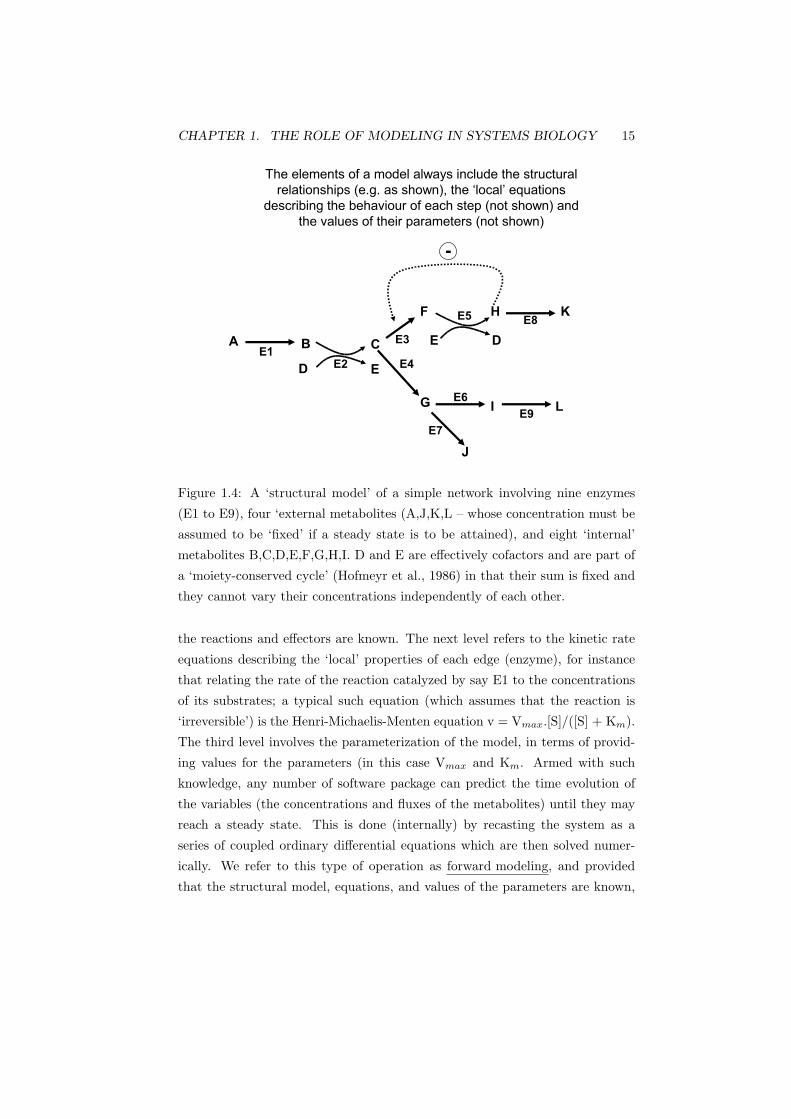
Figure 1.4: A ‘structural model’ of a simple network involving nine enzymes

(E1 to E9), four ‘external metabolites (A,J,K,L – whose concentration must be

assumed to be ‘fixed’ if a steady state is to be attained), and eight ‘internal’

metabolites B,C,D,E,F,G,H,I. D and E are effectively cofactors and are part of

a ‘moiety-conserved cycle’ (Hofmeyr et al., 1986) in that their sum is fixed and

they cannot vary their concentrations independently of each other.

the reactions and effectors are known. The next level refers to the kinetic rate

equations describing the ‘local’ properties of each edge (enzyme), for instance

that relating the rate of the reaction catalyzed by say E1 to the concentrations

of its substrates; a typical such equation (which assumes that the reaction is

‘irreversible’) is the Henri-Michaelis-Menten equation v = Vmax.[S]/([S] + Km).

The third level involves the parameterization of the model, in terms of provid-

ing values for the parameters (in this case Vmax and Km. Armed with such

knowledge, any number of software package can predict the time evolution of

the variables (the concentrations and fluxes of the metabolites) until they may

reach a steady state. This is done (internally) by recasting the system as a

series of coupled ordinary differential equations which are then solved numer-

ically. We refer to this type of operation as forward modeling, and provided

that the structural model, equations, and values of the parameters are known,


it is comparatively easy to produce such models and compare them with an

experimental reality. We have been involved with the simulator Gepasi, written

by Pedro Mendes (Mendes, 1997; Mendes & Kell, 1998; Mendes & Kell, 2001),

which allows one to do all of the above, and that in addition permits automated

variation of the parameters with which to satisfy an objective function such as

the attainment of a particular flux in the steady state (Mendes & Kell, 1998).

In such cases, however, the experimental data that are most readily available

do not include the parameters at all, and are simply measurements of the (time-

dependent) variables, of which fluxes and concentrations are the most common

(see Chapter ch9). Comparison of the data with the forward model is much

more difficult, as we have to solve an ‘inverse modeling’, ‘reverse engineering’

or ‘system identification’ (Ljung, 1999) problem (discussed in Chapter ch10).

Direct solution of such problems is essentially impossible, as they are normally

hugely underdetermined and do not have an analytical solution. The normal

approach is thus an iterative one in which a candidate set of parameters is pro-

posed, the system run in the forward direction, and on the basis of some metric

of closeness to the desired output a new set of parameters is tested. Eventually

(assuming that the structural model and the equations are adequate), a satisfac-

tory set of parameter, and hence solutions, will be found (see Table 1.1). These

methods are much more computer-intensive than those required for simple for-

ward modeling, as potentially many thousands or even millions of candidate

models must be tested. Modern approaches to inverse modeling use approaches

from heuristic optimization (Corne et al., 1999) to search the model space ef-

ficiently. Recent advances in multiobjective optimization (Fonseca & Fleming,

1996) are particularly promising in this regard, since the quality of a model can

usually be evaluated only by considering several, often conflicting criteria. Evo-

lutionary computation approaches (Deb, 2001) allow exploration of the Pareto

front, that is the different trade-offs (e.g. between model simplicity and accu-

racy) that can be achieved, enabling the modeler to make more informed choices

about preferred solutions.

We note, however, that there are a number of other modeling strategies and

issues that may lead one to wish to choose different types of model from that

described. First, the ODE model assumes that compartments are well stirred

and that the concentrations of the participants are sufficiently great as to permit

fluctuations to be ignored. If this is not the case then stochastic simulations (SS)


Table 1.1: 10 Steps in (Inverse) Modeling.

1. Get acquainted with the target system to be modeled

2. Identify important variable(s) that changes over time

3. Identify other key variables and their interconnections

4. Decide what to measure and collect data

5. Decide on the form of model and its architecture

6. Construct a model by specifying all parameters. Run the model

forward and measure behavior.

7. Compare model with measurements. If model is improving re-

turn to 6. If model is not improving and not satisfactory, return

to 3, 4, and 5.

8. Perform sensitivity analysis. Return to 6 and 7 if necessary.

9. Test the impact of control policies, initial conditions, etc.

10. Use multicriteria decision-making (MCDM) to analyze policy

tradeoffs.

are required (Andrews & Bray, 2004) (which are topics of Chapter ch8 and

Chapter 15). If flow of substances between many contiguous compartments

is involved, and knowledge of the spatial dynamics is required (as is common

in computational fluid dynamics), Partial Differential Equations (PDEs) are

necessary. SS and PDE models are again much more computationally intensive,

although in the latter case the designation of a smaller subset of representative

compartments may be effective (Mendes & Kell, 2001).

If the equations and parameters are absent, it may prove fruitful to use qual-

itative models (Hunt et al., 1993), in which only the direction of change (and

maybe rate of change) is recorded, in an attempt to constrain the otherwise

huge search space of possible structural models (see Chapter ch5). Similarly

models may invoke discrete or continuous time, they may be macro or micro,

and models may be at a single level (e.g. metabolism, signaling) or at multiple

levels (in which the concentrations of metabolites affect gene expression and

vice versa (ter Kuile & Westerhoff, 2001). Models may be top-down (involving

large ‘blocks’) or bottom-up (based on elementary reactions), and analyses ben-

eficially use both strategies (Fig. 1.3). Thus a ‘middle-out’ strategy is preferred

by some authors (Noble, 2003) (see Chapter ch14). Table 1.2 sets out some of


the issues in terms of choices which the modeler may face in deciding which type

of model may be best for particular purposes and on the basis of the available

amount of knowledge of the system.

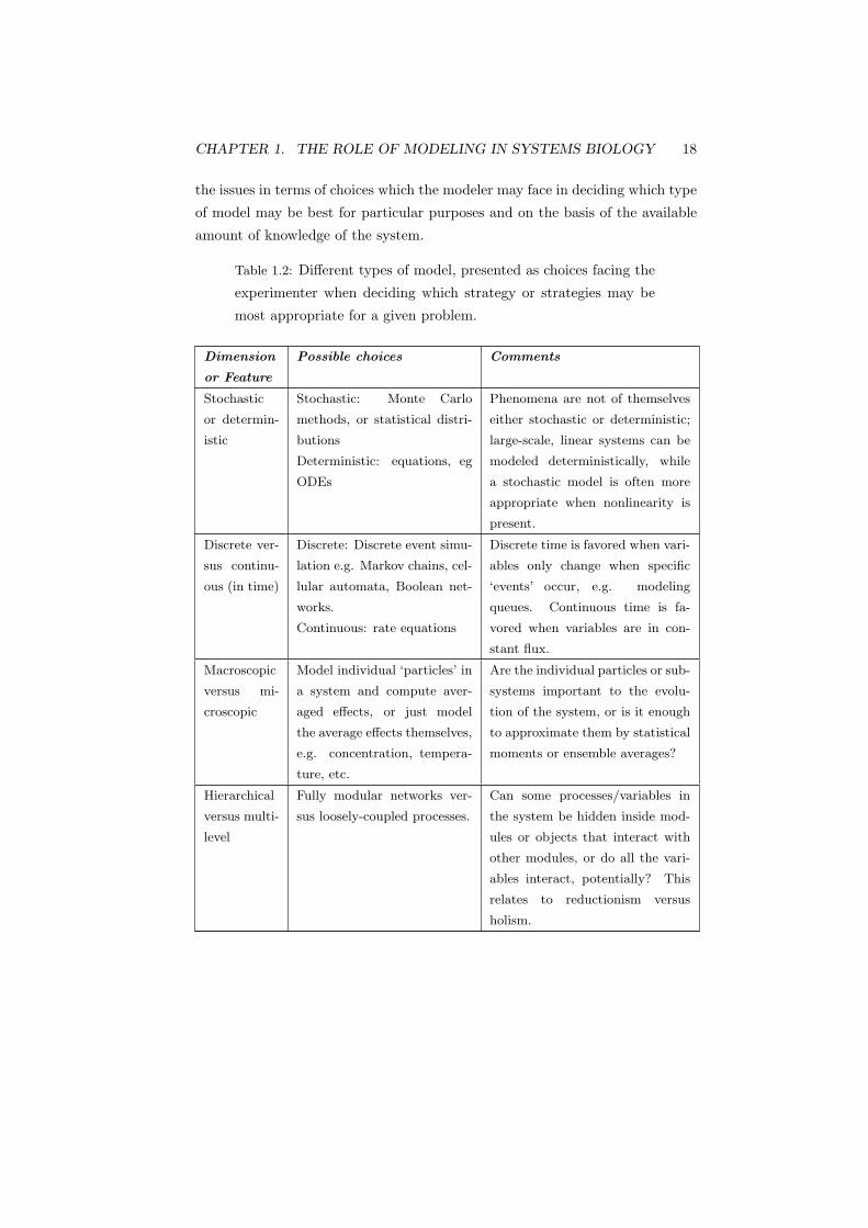
Table 1.2: Different types of model, presented as choices facing the

experimenter when deciding which strategy or strategies may be

most appropriate for a given problem.

Dimension

or Feature

Possible choices Comments

Stochastic

or determin-

istic

Stochastic: Monte Carlo

methods, or statistical distri-

butions

Deterministic: equations, eg

ODEs

Phenomena are not of themselves

either stochastic or deterministic;

large-scale, linear systems can be

modeled deterministically, while

a stochastic model is often more

appropriate when nonlinearity is

present.

Discrete ver-

sus continu-

ous (in time)

Discrete: Discrete event simu-

lation e.g. Markov chains, cel-

lular automata, Boolean net-

works.

Continuous: rate equations

Discrete time is favored when vari-

ables only change when specific

‘events’ occur, e.g. modeling

queues. Continuous time is fa-

vored when variables are in con-

stant flux.

Macroscopic

versus mi-

croscopic

Model individual ‘particles’ in

a system and compute aver-

aged effects, or just model

the average effects themselves,

e.g. concentration, tempera-

ture, etc.

Are the individual particles or sub-

systems important to the evolu-

tion of the system, or is it enough

to approximate them by statistical

moments or ensemble averages?

Hierarchical

versus multi-

level

Fully modular networks ver-

sus loosely-coupled processes.

Can some processes/variables in

the system be hidden inside mod-

ules or objects that interact with

other modules, or do all the vari-

ables interact, potentially? This

relates to reductionism versus

holism.


Table 1.2: Different types of model, presented as choices facing the

experimenter when deciding which strategy or strategies may be

most appropriate for a given problem.

Dimension

or Feature

Possible choices Comments

Fully quanti-

tative versus

partially

quantita-

tive versus

qualitative

Qualitative: direction of

change modeled only, or

on/off states (Boolean net-

work)

Partially quantitative: fuzzy

models

Fully quantitative: ODEs,

PDEs, microscopic particle

models

Reducing the quantitative accu-

racy of the model can reduce com-

plexity greatly and many phenom-

ena may still be modeled ade-

quately.

Predictive

versus ex-

ploratory /

explanatory

Predictive: specify every vari-

able that could affect outcome

Exploratory: only consider

some variables of interest

If a model is being used for pre-

cise prediction or forecasting of a

future event, all variables need to

be considered. The exploratory

approach can be less precise but

should be more flexible, e.g. al-

lowing different control policies to

be tested.

Estimating

rare events

versus typi-

cal behavior

Rare events: Importance sam-

pling

Estimation of rare events, such

as apoptosis times in cells? Is

time-consuming if standard Monte

Carlo simulation is used. Impor-

tance sampling can be used to

‘speed up’ the simulation.

Lumped or

spatially

segregated

Are compartments e.g. cells

to be treated as homoge-

neous or differentiated/ het-

erogeneous?

If heterogeneous it may be nec-

essary to use the computationally

intensive partial differential equa-

tion, though other solutions are

possible (Mendes & Kell, 2001)


1.5 Sensitivity Analysis

-Sensitivity analysis for modelers?

-Would you go to an orthopaedist who didn’t use X-ray?

Jean-Marie Furbringer

Sensitivity analysis (Saltelli et al., 2000) represents a cornerstone in our

analysis of complex systems. It asks the generalized question ‘what is the effect

of changing something (a parameter P) in the model on the behavior of some

variable element M of the model?’. To avoid the magnitude of the answer

depending on the units used we use fractional changes ∆P and observe their

effects via fractional changes (∆M) in M. Thus the generalized sensitivity is

(∆M/M)/(∆P/P) and in the limit of small changes (where the sensitivity is

then independent of the size of ∆P) the sensitivity is (dM/M)/(dP/P) = d

lnM/ dlnP. The sensitivities are thus conceptually and numerically the same as

the control coefficients of Metabolic Control Analysis (see (Fell, 1996; Heinrich

& Schuster, 1996; Kell & Westerhoff, 1986)).

Reasons for doing sensitivity analysis include the ability to determine:

1. if a model resembles the system or process under study

2. factors that may contribute to output variability and so need the most

consideration

3. the model parameters that can be eliminated if one wishes to simplify the

model wihtout altering its behavior grossly

4. the region in the space of input variables for which model variation is

maximum

5. the optimal region for use in a calibration study

6. if and which group of factors interact with each other.

A basic prescription for perform sensitivity analysis (adapted from (Saltelli

et al., 2000)) is:

1. Identify the purpose of the model and determine which variables should

concern the analysis


2. Assign ranges of variation to each input variable

3. Generate an input vector matrix through an appropriate design (DoE)

4. Evaluate the model, thus creating an output distribution or response.

5. Assess the influence of each variable or group of variables e.g. using cor-

relation/regression, Bayesian inference (Chapter ch4), machine learning

or other.

Two examples from our recent work illustrate some of these issues. In the

first, (Nelson et al., 2004; Ihekwaba et al., 2004), we studied a refined version

of a model (Hoffmann et al., 2002) of the NF-κB pathway. This contained 64

reactions with their attendant parameters, but sensitivity analysis showed that

only 8-9 of them exerted significant influence on the dynamics of the nuclear

concentration of NF-κB in this system, and that each of these reactions involved

free IκBα and free IKK. An entirely different study (White & Kell, 2004) asked

whether comparative genomics and experimental data could be used to rank

candidate gene products in terms of their utility as antimicrobial drug targets.

The contribution of each of the sub-metrics (such as essentiality, or existence

only in pathogens and not hosts or commensals) to the overall metric was ana-

lyzed by sensitivity analysis using 3 different weighting functions, with the ‘top

3 targets’ – which were quite different from those of traditional antibiotics –

being similar in all cases. This gave much confidence in the robustness of the

conclusions drawn.

1.6 Concluding remarks

The purpose of this chapter was to give an overview of some of the reasons

for seeking to model complex cellular biological systems, and this we trust

that we have done. We have also given a very brief overview of some of the

methods, but we have not dwelt in detail on: their differences, the question of

which modeling strategies to exploit in particular cases, the problems of overde-

termination (where many models can fit the same data) and of model choice

(which model one might then prefer and why), nor on available models (e.g. at

http://www.biomodels.net/) and model exchange using e.g. the Systems Biol-

ogy Markup Language (http://www.sbml.org) (Finney & Hucka, 2003; Hucka


et al., 2003; Shapiro et al., 2004) or others (Lloyd et al., 2004). These issues are

all covered well in the other chapters of this book.

Finally, we note here that despite the many positive advantages of the mod-

eling approach, biologists are generally less comfortable with, and confident in,

models (and even theories) than are practitioners in some other fields where

this is more of a core activity, e.g. physics or engineering. Indeed, when Ein-

stein was once informed that an experimental result disagreed with his theory

of relativity, he famously and correctly remarked “Well, then, the experiment

is wrong!” It is our hope that trust will grow, not only from a growing number

of successful modeling endeavors, but also from a greater and clearer commu-

nication of models enabled by new technologies such as Web services and the

SBML.

1.7 Acknowledgments

We thank the BBSRC and EPSRC for financial support, and Dr Neil Benson,

Prof Igor Goryanin, Dr Edda Klipp and Dr Joerg Stelling for useful discussions.

Bibliography

Andrews, S. & Bray, D. (2004). Stochastic simulation of chemical reactions with

spatial resolution and single molecule detail. Phys Biol 1, 137–51.

Angeli, D., Ferrell, Jr., J. & Sontag, E. (2004). Detection of multistability,

bifurcations, and hysteresis in a large class of biological positive-feedback

systems. Proc. Natl. Acad. Sci. U.S.A. 101, 1822–27.

Arthur, B. (1963). On generalized urn schemes of the polya kind. Cybernetics

19, 61–71.

Barabasi, A.-L. & Albert, R. (1999). Emergence of scaling in random networks.

Science 286, 509–12.

Bohm, H.-J. & Schneider, G., eds (2000). Virtual screening for bioactive

molecules. Wiley-VCH, Weinheim.

Bynum, W. F., Browne, E. & Porter, R., eds (1981). Dictionary of the history

of science. MacMillan Press, London.

Cascante, M., Boros, L. G., Comin-Anduix, B., de Atauri, P., Centelles, J. J.

& Lee, P. W.-N. (2002). Metabolic control analysis in drug discovery and

disease. Nat. Biotechnol. 20, 243–9.

Corne, D., Dorigo, M. & Glover, F., eds (1999). New Ideas in Optimization.

McGraw-Hill.

Cornish-Bowden, A. (1999). Metabolic control analysis in biotechnology and

medicine. Nat. Biotechnol. 17, 641–43.

23

BIBLIOGRAPHY 24

Davey, H. & Kell, D. (1996). Flow cytometry and cell sorting of heterogeneous

microbial populations: the importance of single-cell analysis. Microbiol.

Rev. 60, 641–96.

Davies, P. (2004). Emergent biological principles and the computational prop-

erties of the universe. Complexity 11, 11–15.

Deb, K. (2001). Multi-Objective Optimization using Evolutionary Algorithms.

John Wiley & Sons, Chichester.

Elowitz, M. & Leibler, S. (2000). A synthetic oscillatory network of transcrip-

tional regulators. Nature 403, 335–38.

Fell, D. (1996). Understanding the control of metabolism. Portland Press,

London.

Fell, D. (1998). Increasing the flux in metabolic pathways: a metabolic control

analysis perspective. Biotechnol Bioeng 58, 121–24.

Finney, A. & Hucka, M. (2003). Systems biology markup language: Level 2 and

beyond. Biochem Soc Trans 31, 1472–3.

Fonseca, C. & Fleming, P. (1996). Nonlinear system identification with multiob-

jective genetic algorithms. In Proceedings of the 13th World Congress of the

International Federation of Automatic Control pp. 187–92,, San Francisco,

California.

Gilbert, G. & Mulkay, N. (1984). Opening Pandora’s box : a sociological analysis

of scientists’ discourse. Cambridge University Press, Cambridge.

Glendinning, P. (1994). Stability, Instability and Chaos: An Introduction to the

Theory of Nonlinear Differential Equations. Cambridge University Press,

Cambridge.

Goldberg, D. (2002). The design of innovation: lessons from and for competent

genetic algorithms. Kluwer, Boston.

Heinrich, R. & Schuster, S. (1996). The regulation of cellular systems. Chapman

& Hall, New York.

BIBLIOGRAPHY 25

Hoffmann, A., Levchenko, A., Scott, M. L. & Baltimore, D. (2002). The

IkappaB-NF-kappaB signaling module: temporal control and selective gene

activation. Science 298, 1241–5.

Hofmeyr, J., Kacser, H. & van der Merwe, K. (1986). Metabolic control analysis

of moiety-conserved cycles. Eur J Biochem 155, 631–41.

Hofstadter, D. (1979). Godel, Escher, Bach: an eternal golden braid. Basic

Books, New York.

Holland, J. (1998). Emergence. Helix, Reading, MA.

Hucka, M., Finney, A., Sauro, H., Bolouri, H., Doyle, J., Kitano, H., Arkin,

A., Bornstein, B., Bray, D., Cornish-Bowden, A., Cuellar, A., Dronov, S.,

Gilles, E., Ginkel, M., Gor, V., Goryanin, I., Hedley, W., Hodgman, T.,

Hofmeyr, J., Hunter, P., Juty, N., Kasberger, J., Kremling, A., Kummer,

U., Novere, N. L., Loew, L., Lucio, D., Mendes, P., Minch, E., Mjolsness, E.,

Nakayama, Y., Nelson, M., Nielsen, P., Sakurada, T., Schaff, J., Shapiro,

B., shimizu, T., Spence, H., Stelling, J., Takahashi, K., Tomita, M., Wag-

ner, J. & Wang, J. (2003). The Systems Biology Markup Language (SBML):

a medium for representation and exchange of biochemical network models.

Bioinformatics 19, 524–31.

Hunt, J., Lee, M. & Price, C. (1993). Applications of qualitative model-based

reasoning. Control Eng. Pract. 1, 253–66.

Ihekwaba, A., Broomhead, D., Grimley, R., Benson, N. & Kell, D. (2004).

Sensitivity analysis of parameters controlling oscillatory signalling in the

NF-κB pathway: the roles of IKK and IκBα. IEE Systems Biol 1, 93–103.

Johnson, N. L. & Kotz, S. (1977). Urn models and their application : an

approach to modern discrete probability theory. Wiley.

Johnson, S. (2001). Emergence. Scribner, New York.

Kauffman, S. (2000). Investigations. Oxford University Press, Oxford.

Kauffman, S., Lobo, J. & Macready, W. (2000). Optimal search on a technology

landscape. J Econ Behav Organ 43, 141–66.

BIBLIOGRAPHY 26

Kell, D. (2004). Metabolomics and systems biology: making sense of the soup.

Curr. Opin. Microbiol. 7, 296–307.

Kell, D. (2005). Metabolomics, machine learning and modelling: towards an

understanding of the language of cells. Biochem. Soc. Trans. 33. in the

press.

Kell, D. & King, R. (2000). On the optimization of classes for the assignment of

unidentified reading frames in functional genomics programmes: the need

for machine learning. Trends Biotechnol 18, 93–8.

Kell, D. & Welch, G. (1991). No turning back, reductonism and biological

complexity. Times Higher Educational Supplement 9th August, 15.

Kell, D. & Westerhoff, H. (1986). Metabolic control theory: its role in microbi-

ology and biotechnology. FEMS Microbiol Rev 39, 305–20.

Kell, D. B. (2002). Genotype:phenotype mapping: genes as computer programs.

Trends Genet. 18, 555–559.

Kell, D. B. & Oliver, S. G. (2004). Here is the evidence, now what is the

hypothesis? The complementary roles of inductive and hypothesis-driven

science in the post-genomic era. Bioessays 26, 99–105.

Klebe, G., ed. (2000). Virtual screening: an alternative or complement to high-

throughput screening. Kluwer Academic Publishers, Dordrecht.

Klipp, E., Herwig, R., Kowald, A., Wierling, C. & Lehrach, H. (2005). Systems

Biology in Practice: Concepts, Implementation and Clinical Application.

Wiley-VCH, Berlin.

Lahav, G., Rosenfeld, N., Sigal, A., Geva-Zatorsky, N., Levine, A. J., Elowitz,

M. B. & Alon, U. (2004). Dynamics of the p53-Mdm2 feedback loop in

individual cells. Nat Genet 36, 147–50.

Langer, T. & Hoffmann, R. (2001). Virtual screening: an effective tool for lead

structure discovery? Current Pharmaceutical Design 7, 509–527.

Lipton, P. (2005). Testing hypotheses: prediction and prejudice. Science 307,

219–21.

BIBLIOGRAPHY 27

Ljung, L. (1999). System identification : theory for the user. 2nd edition,

Prentice Hall PTR, Upper Saddle River, NJ.

Lloyd, C. M., Halstead, M. D. B. & Nielsen, P. F. (2004). CellML: its future,

present and past. Prog Biophys Mol Biol 85, 433–50.

ter Kuile, B. & Westerhoff, H. (2001). Transcriptome meets metabolome: hi-

erarchical and metabolic regulation of the glycolytic pathway. FEBS Lett.

500, 169–71.

Medawar, P. (1982). Pluto’s republic. Oxford University Press, Oxford.

Mendes, P. (1997). Biochemistry by numbers: simulation of biochemical path-

ways with Gepasi 3. Trends Biochem Sci 22, 361–3.

Mendes, P. & Kell, D. (1998). Non-linear optimization of biochemical pathways:

applications to metabolic engineering and parameter estimation. Bioinfor-

matics 14, 869–83.

Mendes, P. & Kell, D. (2001). MEG (Model Extender for Gepasi): a program for

the modelling of complex, heterogeneous, cellular systems. Bioinformatics

17, 288–9.

Milo, R., Shen-Orr, S., Itzkovitz, S., Kashtan, N., Chklovskii, D. & Alon, U.

(2002). Network motifs: simple building blocks of complex networks. Sci-

ence 298, 824–27.

Morowitz, H. J. (2002). The Emergence of Everything. Oxford University Press,

Oxford.

Nagel, E. & Newman, J. (2002). Godel’s proof. New York University Press,

New York.

Nelson, D., Ihekwaba, A. E. C., Elliott, M., Johnson, J., Gibney, C., Foreman,

B., Nelson, G., See, V., Horton, C., Spiller, D., Edwards, S., McDowell, H.,

Unitt, J., Sullivan, E., Grimley, R., Benson, N., Broomhead, D., Kell, D.

& White, M. R. H. (2004). Oscillations in NF-kappaB signaling control the

dynamics of gene expression. Science 306, 704–8.

Noble, D. (2003). The future: putting Humpty-Dumpty together again.

Biochem Soc Trans 31, 156–8.

BIBLIOGRAPHY 28

Ogata, K. (2001). Modern Control Engineering. Prentice Hall.

Pomerening, J., Sontag, E. & Ferrell Jr., J. (2003). Building a cell cycle oscil-

lator: hysteresis and bistability in the activation of Cdc2. Nat. Cell Biol.

5, 346–51.

Popper, K. (1992). Conjectures and refutations: the growth of scientific knowl-

edge. 5th ed. edition, Routledge & Kegan Paul, London.

Pritchard, L. & Kell, D. B. (2002). Schemes of flux control in a model of

Saccharomyces cerevisiae glycolysis. Eur J Biochem 269, 3894–904.

Saltelli, A., Chan, K. & Scott, E., eds (2000). Sensitivity analysis. Wiley,

Chichester.

Shapiro, B. E., Hucka, M., Finney, A. & Doyle, J. (2004). MathSBML: a

package for manipulating SBML-based biological models. Bioinformatics

20, 2829–31.

Shen, J., Xu, X., Cheng, F., Liu, H., Luo, X., Chen, K., Zhao, W., Chen, X.

& Jiang, H. (2003). Virtual screening on natural products for discovering

active compounds and target information. Curr Med Chem 10, 2327–42.

Sole, R. & Goodwin, B. (2000). Signs of life: how complexity pervades biology.

Basic Books, New York.

Strogatz, S. (2000). Nonlinear Dynamics and Chaos: With Applications to

Physics, Biology, Chemistry and Engineering. Perseus Publishing.

Tufillaro, N. B., Abbott, T. & Reilly, J. (1992). An Experimental Approach to

Nonlinear Dynamics and Chaos. Perseus Publishing.

Tyson, J., Chen, K. & Novak, B. (2003). Sniffers, buzzers, toggles and blinkers:

dynamics of regulatory and signaling pathways in the cell. Curr. Opin. Cell

Biol. 15, 221–31.

Westerhoff, H. & Kell, D. (1987). Matrix method for determining the steps most

rate-limiting to metabolic fluxes in biotechnological processes. Biotechnol

Bioeng 30, 101–07.

White, T. & Kell, D. (2004). Comparative genomic assessment of novel broad-

spectrum targets for antibacterial drugs. Comp Func Genomics 5, 304–27.

BIBLIOGRAPHY 29

Wolf, D. & Arkin, A. (2003). Motifs, modules and games in bacteria. Curr.

Opin. Microbiol. 6, 125–34.

Yeger-Lotem, E., Sattath, S., Kashtan, N., Itzkovitz, S., Milo, R., Pinter, R.,

Alon, U. & Margalit., H. (2004). Network motifs in integrated cellular

networks of transcription-regulation and protein-protein interaction. Proc.

Natl. Acad. Sci. U.S.A. 101, 5934–39.

Zanders, E., Bailey, D. & Dean, P. (2002). Probes for chemical genomics by

design. Drug Discovery Today 7, 711–18.

The role of modeling in systems biology - DBK...

Documents

Transcript of The role of modeling in systems biology - DBK...