The Role of Interbank Markets in Monetary Policy:

A Model with Rationing

Xavier Freixas∗ José Jorge†

Abstract

This paper analyses the impact of asymmetric information in the interbank

market and establishes its crucial role in the microfoundations of the monetary

policy transmission mechanism. We show that interbank market imperfections

We thank an anonymous referee for very helpful comments and suggestions. We are also gratefulto Viral Acharya, Adam Ashcraft, Arturo Estrella, Falko Fecht, Stefan Gerlach, Marvin Goodfriend,Ping He, Don Morgan, Alexandra Niessen, George Pennacchi, Rafael Repullo, David Skeie, JavierSuarez for helpful comments as well as seminar participants at the Second Financial IntermediationResearch Society Conference on Banking, Corporate Finance and Intermediation, CEMFI, DeutscheBundesbank, "The Credit Channel of Monetary Policy in the 21st Century" Conference organizedby the Federal Reserve Bank of Atlanta, Federal Reserve Bank of New York, 22nd Congress of theEuropean Economic Association, "Banking and the Macroeconomy" conference organized by the CEPRand CER-ETH, "Banking and Asset Markets" conference organized by the CEPR, Banque de France andFondation Banque de France, "The Implications of Changes in Banking and Financing for the MonetaryPolicy Transmission Mechanism" conference organized by the European Central Bank, Midwest FinanceAssociation 57th Annual Meeting, and Banca d’Italia for discussions and comments.

∗Professor of Financial Economics, Department of Economics and Business, Universitat PompeuFabra, and Research Fellow at CEPR. Financial support from the Spanish Ministry under grantSEJ2005-03924 is gratefully acknowledged. E-mail: xavier.freixas@upf.edu

†Assistant Professor, CEMPRE and Faculdade de Economia, Universidade do Porto. Centro deEstudos Macroeconómicos e Previsão (CEMPRE) is a research centre supported by Fundação para aCiência e a Tecnologia, which is financed by Portuguese Government funds and by European Unionfunds, within the framework of Programa Operacional Ciência e Inovação 2010. Financial supportfrom Fundação para a Ciência e a Tecnologia - Programa Praxis XXI - III Quadro Comunitário deApoio, sponsored by the European Social Fund together with Ministério da Ciência, Tecnologia e EnsinoSuperior (BD/15698/98) is gratefully acknowledged. E-mail: jjorge@fep.up.pt

1

induce an equilibrium with rationing in the credit market. This has two major

implications: first, it reconciles the irresponsiveness of business investment to the

user cost of capital with the large impact of monetary policy (magnitude effect)

and, second, it shows that banks’ liquidity positions condition their reaction to

monetary policy (Kashyap and Stein liquidity effect).

JEL codes: E44, G21.

Keywords: Banking, Rationing, Monetary Policy.

1 Introduction

The aim of this paper is to understand how financial imperfections in the interbank mar-

ket affect the monetary policy transmission mechanism and, more precisely, to explore

whether the structure of the banking system has any effects beyond those of the classical

money channel.

There are two basic empirical motivations for our work. On the one hand, Kashyap

and Stein (2000) result, showing that the impact of monetary policy on a banks’ amount

of lending is stronger for banks with less liquid balance sheets, establishes the existence

of imperfections in the interbank market. Such a liquidity effect is a challenge to the

theoretical modelling of monetary policy channels based on highly efficient interbank

markets, an assumption justified by the large volumes of transactions and the particularly

low spreads observed on these markets.

On the other hand, the failure of existing theories of monetary transmission to explain

a number of empirical facts has also been a motivation for our work. Bernanke and

Gertler (1995) document that empirical research has been unsuccessful in identifying

a quantitatively important cost of capital effect on private spending, which has been

labeled as the magnitude effect, whereby the aggregate impact of monetary policy is

deemed excessively large, given the small elasticity of firms investment with respect to

their cost of capital.

In this paper we show that, once we allow for interbank market imperfections, not

only can we justify the Kashyap and Stein liquidity effect, but a new framework of

analysis opens up, allowing for a better understanding of the magnitude effect.

3

The interbank market allows banks to cope with liquidity shocks by borrowing and

lending from their peers, a function that, as it is assumed in this paper, the access to

(inelastically supplied) deposits cannot fulfill. Our paper uncovers the important role

of the interbank market in an asymmetric information set-up by establishing the link

between the imperfect functioning of the interbank market and the existence of rationing

of banks and, in a cascading effect, of firms in the credit market. Our modelling of this

effect allows us to establish that the relevance of imperfections in the interbank market

for monetary policy depends on: (i) the dependence of firms on bank finance; (ii) the

extent of relationship lending, in the sense of firms having access to funds through a

unique bank; (iii) the heterogeneity of banks’ liquidity positions, resulting from Treasury

securities (T-Bills) holdings resulting from past decisions and liquidity shocks originated

in additional funding for existing projects.

The existence of credit rationing is of interest in our context because, traditionally,

the theory of credit rationing has been developed in a borrower-lender framework, better

suited to the theory of banking than to the analysis of the transmission mechanism of

monetary policy. In this paper we argue that credit rationing might also be an important

part of the transmission mechanism. Introducing interbank market imperfections in the

analysis of monetary policy seems a reasonable approach for two reasons. First, the

interbank market is the first one to be exposed to the effects of monetary policy in the

chain of effects that will generate the full impact of monetary policy. Second, it is worth

considering an imperfect interbank market because Kashyap and Stein liquidity effect

forces us to reconsider its supposedly perfect functioning and questions its purely passive

4

role.

In order to analyze rigorously the effects of interbank markets imperfections on mone-

tary transmission, we compare the transmission mechanism under two different scenarios:

of symmetric and asymmetric information in the interbank market. The main lesson is

that, under asymmetric information, the interbank market is unable to efficiently channel

liquidity to solvent illiquid banks and, as a consequence, there is quantity rationing in the

bank loan market. The implications of credit rationing for monetary policy are straight-

forward. Under asymmetric information, monetary transmission may not be solely based

on the interest rate channel, but may also depend on a rationing channel. When the

Central Bank tightens its monetary policy, bank deposits decline and banks with less

liquid balance sheets are forced to cut down on their lending. Thus, in an asymmetric in-

formation framework, an effect that cannot be accounted for in a symmetric information

framework occurs: the interest rate effects combine with those of credit rationing and

reinforce one another. This combination explains why the effect of a monetary policy

shock is larger than the one purely caused by interest rate movements, thus providing a

justification for the magnitude effect.

Our paper is related to several strands of the literature. As mentioned, our motivation

stems from a number of empirical findings resulting from the concern with the traditional

view of monetary policy, the money view, which explains the effects of monetary policy

through the interest rate channel. Confronting this view, the broad credit channel, in

its different variants (based either on the firms balance sheet and credit risk or on the

banks’ inability to extend credit) assigns a more pre-eminent role to banks and asserts

5

that the supply of credit plays a key role on the impact of monetary policy. One of

its variants, the lending view, has focussed on the role of bank loans (Kashyap, Stein,

and Wilcox 1993, were the first to clearly identify shifts in bank loan supply and to

show that there is indeed a bank lending channel). Complementing the criticism to the

interest rate channel, Mihov (2001) presents evidence that the banking system plays

an important role in the propagation of monetary policy. Namely, he shows that the

magnitude of monetary policy responses of aggregate output is larger for countries with

a higher ratio of corporate bank loans to total liabilities. Moreover, he uses measures of

banking industry health to conclude that the magnitude of monetary policy is larger for

countries with less healthy banking systems, that is, that are subject to higher levels of

financial imperfection. These are issues that a rigorous modeling of the banking sector

should be able to clarify.

The lending view rests on the claim that there is a significant departure from the

Modigliani-Miller Theorem for the banking firm, because financial markets are character-

ized by asymmetric information. When the Central Bank tightens its monetary policy,

it forces banks to substitute away from reservable insured deposit financing and towards

adverse-selection-prone forms of non-deposit financing. This portfolio reallocation leads

banks to adjust their asset holdings and this leads to a shift in the bank loan supply

schedule, as argued by Stein (1998). Adopting such a perspective leads naturally to

a theory of the spread - augmented interest rate channel. Some authors have indeed

highlighted the influence of monetary innovations on the spread between the interest

rate on bank loans and the risk free rate to justify the relevance of banks for monetary

6

policy (see Kashyap and Stein 1994, and Stein 1998). However, empirical research has

faced great difficulties in showing that a contractionary monetary policy will increase the

spread on bank loans. Berger and Udell (1992) document that, on the contrary, bank

loan rate premia over treasury rates of equal duration decrease substantially when Trea-

sury securities rates increase (and commitment loans do not explain this phenomenon),

contrarily to the theoretical prediction.

A second strand of the empirical literature on monetary policy that is directly rele-

vant for our analysis is concerned with the magnitude effect. On the one hand, it has

been extensively reported that the response of business investment to the user cost of

capital tends to be unimportant relative to quantity variables, like financial structure and

cash flow. These variables have been included frequently as regressors in estimations,

and generally have proven significant, suggesting that investment depends on variables

other than the user cost of capital.1 On the other hand, the empirical research on the

macroeconomic effects of shifts in the interest rates controlled by the Central Bank shows

that the real economy is powerfully affected by monetary policy innovations that induce

relatively small movements in policy rates. See Angeloni et al. (2002) for additional

empirical evidence on the magnitude effect in Europe.

According to Bernanke and Gertler (1995), most monetary models predict that mone-

tary policy should have its strongest influence on short-term interest rates and a relatively

weaker impact on (real) long-term rates. Yet, the empirical evidence shows that the most

1See Hubbard (1998) and Schiantarelli (1995) for a review of this literature. Following the work byKaplan and Zingales (1997) and Cleary (1999), some authors have argued that investment cash flowsensitivity may not be always interpreted as revealing the existence of financial constraints becauseinvestment demand is difficult to measure and may be positively correlated with cash flow.

7

rapid and strongest effect of monetary policy is on residential investment. This finding

is surprising because residential investment is typically very long lived and therefore

should not be sensitive to short term interest rates. This result has been labeled as the

composition effect and we also advance a possible explanation for such effect.

Finally, our paper is related to the borrower-lender relationship under asymmetric

information and to the classical work of Stiglitz and Weiss (1981). Still, we do not

consider second order stochastic dominance, so that our set-up is closer to Ackerloff

(1970)’s market for lemons: once the interbank market is shown to be thin, in the sense

that only fully collateralized loans are made in equilibrium, liquidity short banks are

rationed and are forced to ration their clients.

The borrower-lender relationship under asymmetric information has been also ex-

plored in order to model interbank markets. Not surprisingly, many authors suggest

that the interbank markets deliver an efficient allocation of bank reserves within the

banking system (see, e.g., Goodfriend and King 1988, and Schwartz 1992). This will

be the case if market participants are well informed to assess the solvency of any po-

tential borrower. Still, under asymmetric information, the interbank market may lead

to a second best allocation of liquidity as illustrated by Bhattacharya and Gale (1987),

Rochet and Tirole (1996), Flannery (1996) and Freixas and Holthausen (2005). The

empirical evidence tends to support the asymmetric information view of the market, as

shown by Furfine (2001), who presents evidence that some monitoring is done by lenders

in the interbank market, and Furfine (1999) and Cocco, Gomes, and Martins (2003),

who document the existence of relationship lending in the interbank market. Ashcraft

8

and Bleakley (2006) collect both public and private information about bank loan portfo-

lio quality, and investigate how access to the federal funds market is affected by adverse

changes in the measures of private and public information of loan portfolio quality. They

confirm that the market responds to adverse changes in the public measures of loan port-

folio quality. In addition, they find evidence that banks exploit adverse changes in the

private measure of loan portfolio quality by increasing demand in a fashion consistent

with moral hazard, increasing the frequency of borrowing and liquidity risk in response

to adverse private information.

The paper is organized as follows. We devote the next section to present the basic

model and assumptions. We proceed by comparing the equilibrium under perfect infor-

mation and asymmetric information. Section 6 evaluates the implications of our model

for the monetary transmission mechanism and is followed by a short conclusion.

2 The Model

This section presents a partial equilibriummodel of the bank loan and interbank markets.

Firms face liquidity shocks and rely on bank credit to raise external finance. In this

way the firms’ shocks become a demand for credit and a liquidity shock for the banks.

As in Holmstrom and Tirole (1998) and Stein (1998), banks hold a large fraction of

their assets as reserves and liquid securities to act as a buffer against liquidity shocks.2

We assume that banks hold different amounts of securities and face different liquidity

2Models of how this buffer is build and how it is affected by monetary policy were studied by Stein(1998) and Van den Heuvel (2006).

9

shocks. Owing to heterogeneity, there is a role for an interbank market to trade reserves

as in Battacharya and Gale (1987). We begin by developing a simple model in a perfect

information set-up, and then proceed to introduce asymmetric information on the banks’

liquidity shocks.

Following the literature on monetary macroeconomics, we adopt a highly stylized

view of how monetary authorities implement their policies. The Central Bank sets an

interest rate at which it is willing to borrow or lend unlimited amounts of collateralized

funds, with the collateral being liquid risk free assets as, for example, T-Bills. We call

this interest rate the policy rate and denote it by r, with r ≥ 0. We assume that

households and firms hold money in the form of bank deposits which earn zero interest

and provide payment services.3 The alternative to holding money is holding T-Bills. We

assume that arbitrage guarantees that the interest rate on treasuries equals r. Hence the

Central Bank, by controlling the interest rate, is able to affect the opportunity cost of

holding deposits and we have a standard money demand which depends negatively on

the risk free rate.

2.1 Firms

There is a continuum of firms with unit mass and there are three dates. The sequence

of events and decisions, summarized in Table 1, is as follows. Each firm has a fixed size

project requiring an investment of one unit at date zero. At date one, each firm suffers

3The zero interest rate on retail deposits would be obtained if banks benefit from local monopolypower, the supply of bank deposits is sufficiently inelastic with respect to the deposit rate and interestrates are restricted to be non-negative.

10

Period 0 Period 1 Period 2

- Firms borrow 1 unit

from banks and estab-

lish a credit line for pe-

riod 1.

- The liquidity shock ν is realized.

- If the shock is below a cer-

tain threshold, then the firm

obtains additional financ-

ing F with interest rate rF .

If the shock is above the threshold,

the bank takes over the firm.

- If the firm still oper-

ates, it generates output

Y and pays back to the

bank the amount R0 +

(1 + rF )F .

Table 1: Timing of decisions and events for the firm.

a real shock and needs an amount ν of funds. When ν < 0 the project generates a

revenue for the firm and when ν > 0 the firm experiences a cost overrun. For the sake of

simplification, we also assume that firms can only be financed by bank loans and that, if

the cost overrun is met, the project generates a certain return Y at date two; if it is not

funded, the project is terminated and has no residual value. We assume that the variable

ν is identically and independently distributed across firms with a uniform distribution

with support [ν, ν], ν ≤ 0, ν > 0 and ν+ν > 0. At date one, the firm obtains an amount

F of funds at an interest rate rF .

We are mainly concerned with the effects occurring at date one, since it is at this point

in time when monetary policy will impact the banks and firms decisions. In particular,

we are interested in computing the firms’ optimal liquidation, their borrowing and the

interest rate sensitivity of their output.

Firms have a passive role as they are willing to borrow the amount of liquidity ν they

require to fund their cost overrun and, therefore, F = ν. At date zero, the firm asks

for a unit loan and promises to repay R0 < Y at date two if its project is successful. In

addition, the firm signs a credit line contract so that the interest rate on the date one

bank loan that the firm demands is not renegotiable.

11

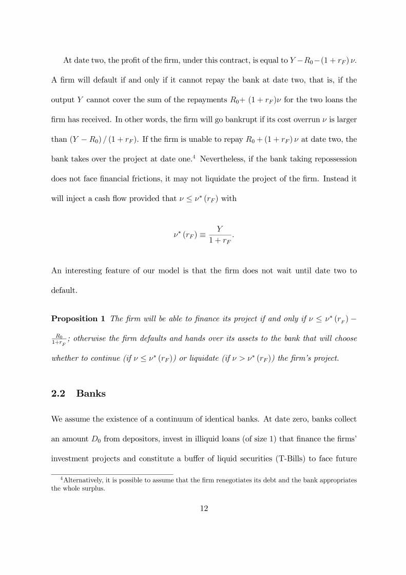
At date two, the profit of the firm, under this contract, is equal to Y −R0−(1 + rF ) ν.

A firm will default if and only if it cannot repay the bank at date two, that is, if the

output Y cannot cover the sum of the repayments R0+ (1 + rF )ν for the two loans the

firm has received. In other words, the firm will go bankrupt if its cost overrun ν is larger

than (Y −R0) / (1 + rF ). If the firm is unable to repay R0 + (1 + rF ) ν at date two, the

bank takes over the project at date one.4 Nevertheless, if the bank taking repossession

does not face financial frictions, it may not liquidate the project of the firm. Instead it

will inject a cash flow provided that ν ≤ ν∗ (rF ) with

ν∗ (rF ) ≡Y

1 + rF.

An interesting feature of our model is that the firm does not wait until date two to

default.

Proposition 1 The firm will be able to finance its project if and only if ν ≤ ν∗ (rF)−

R01+r

F

; otherwise the firm defaults and hands over its assets to the bank that will choose

whether to continue (if ν ≤ ν∗ (rF )) or liquidate (if ν > ν∗ (rF )) the firm’s project.

2.2 Banks

We assume the existence of a continuum of identical banks. At date zero, banks collect

an amount D0 from depositors, invest in illiquid loans (of size 1) that finance the firms’

investment projects and constitute a buffer of liquid securities (T-Bills) to face future

4Alternatively, it is possible to assume that the firm renegotiates its debt and the bank appropriatesthe whole surplus.

12

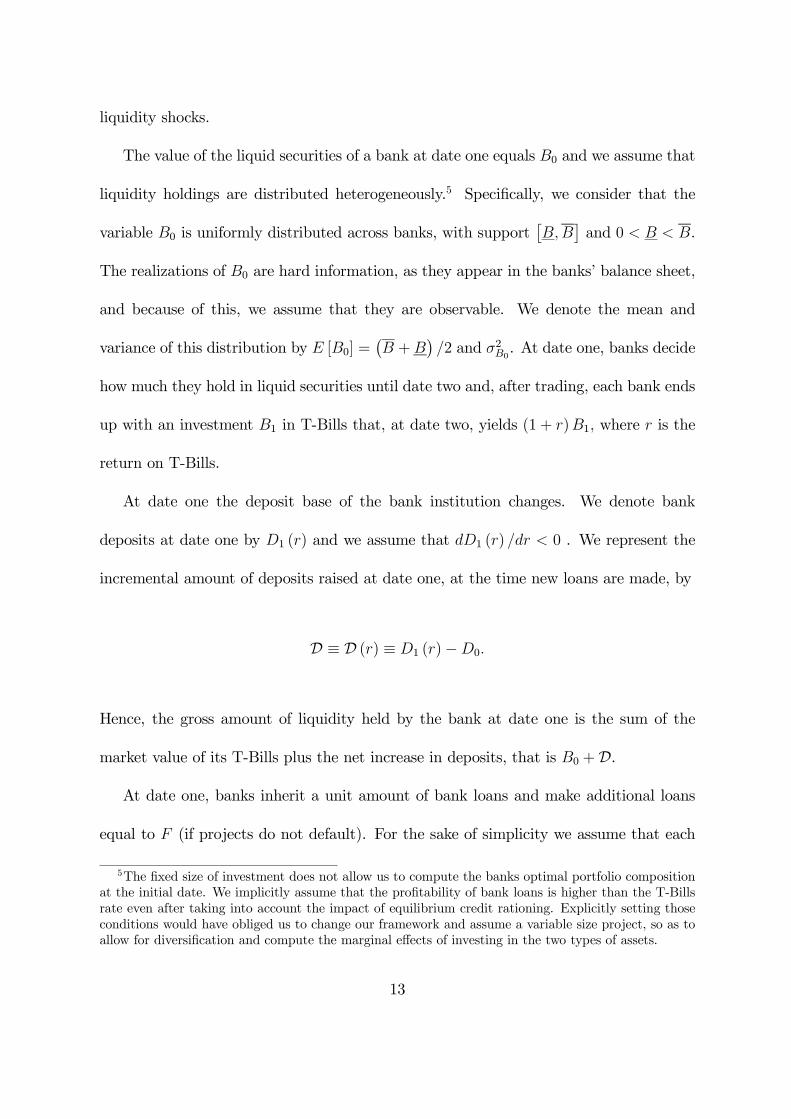
liquidity shocks.

The value of the liquid securities of a bank at date one equals B0 and we assume that

liquidity holdings are distributed heterogeneously.5 Specifically, we consider that the

variable B0 is uniformly distributed across banks, with support[B,B

]and 0 < B < B.

The realizations of B0 are hard information, as they appear in the banks’ balance sheet,

and because of this, we assume that they are observable. We denote the mean and

variance of this distribution by E [B0] =(B +B

)/2 and σ2B0. At date one, banks decide

how much they hold in liquid securities until date two and, after trading, each bank ends

up with an investment B1 in T-Bills that, at date two, yields (1 + r)B1, where r is the

return on T-Bills.

At date one the deposit base of the bank institution changes. We denote bank

deposits at date one by D1 (r) and we assume that dD1 (r) /dr < 0 . We represent the

incremental amount of deposits raised at date one, at the time new loans are made, by

D ≡ D (r) ≡ D1 (r)−D0.

Hence, the gross amount of liquidity held by the bank at date one is the sum of the

market value of its T-Bills plus the net increase in deposits, that is B0 +D.

At date one, banks inherit a unit amount of bank loans and make additional loans

equal to F (if projects do not default). For the sake of simplicity we assume that each

5The fixed size of investment does not allow us to compute the banks optimal portfolio compositionat the initial date. We implicitly assume that the profitability of bank loans is higher than the T-Billsrate even after taking into account the impact of equilibrium credit rationing. Explicitly setting thoseconditions would have obliged us to change our framework and assume a variable size project, so as toallow for diversification and compute the marginal effects of investing in the two types of assets.

13

bank lends funds to a set of firms with perfectly correlated projects. To all purposes

this set of firms is treated as a unique firm, so that there is a one to one correspondence

between the set of firms and the set of banks. Also, we assume a relationship banking

framework so that, on the one hand, a bank has perfect knowledge of the firm liquidity

shock ν, and on the other hand, a firm is captive from that bank and cannot switch

to another one. We justify these assumptions by referring to both theoretical models

and empirical evidence of relationship banking (See, e.g., Boot 2000, for the former and

Degryse and Ongena 2005, for the latter).

The difference between liquid assets and liquid liabilities at date one equals F −

(B0 +D) and will be covered through access to the unsecured interbank market. A

bank’s net borrowing in the interbank market at date one will be denoted by L (positive

or negative) and the corresponding interest rate by rL. This interest rate may incorporate

a risk premium because lenders in the interbank market are exposed to default risk.

Lenders in this market diversify their interbank loan portfolio and obtain an effective

rate of return ρL. Formally, let

γ =

ρL if L < 0

rL if L ≥ 0

with rL ≥ ρL.

In order to avoid multiplicity of equilibria we assume that, when the cost of interbank

funds is equal to the return on treasuries, banks do not borrow in the interbank market

to invest in treasuries. Formally, we assume that LB1 ≤ 0 when rL = r.

The timing of the events for the bank is described in Table 2.

14

Period 0 Period 1 Period 2

- The bank collects re-

tail deposits equal to

D0, lends 1 unit to the

firm and invests in secu-

rities.

- The securities held by the bank

are worth B0. A new amount of

deposits D1(r) is realized.

- The liquidity shock ν of the

firm is realized.

- If the shock is below a certain

threshold, the bank lends an amount

F to the firm at the interest rate rF .

- If the shock is above the threshold,

the bank takes over the firm and de-

cides whether to continue its project

or not. The bank does not continue

the project if the shock is above ν∗.

- If the bank has excess liquidity it

invests in securities or lends in the

interbank markets. Otherwise, it

borrows an amount L in the inter-

bank market at a rate rL.

- If the firm still op-

erates, the bank re-

ceives R0 + (1 + rF )F .

- If the bank is oper-

ating the project of the

firm, it receives Y .

Table 2: Timing of decisions and events for the bank under perfect information.

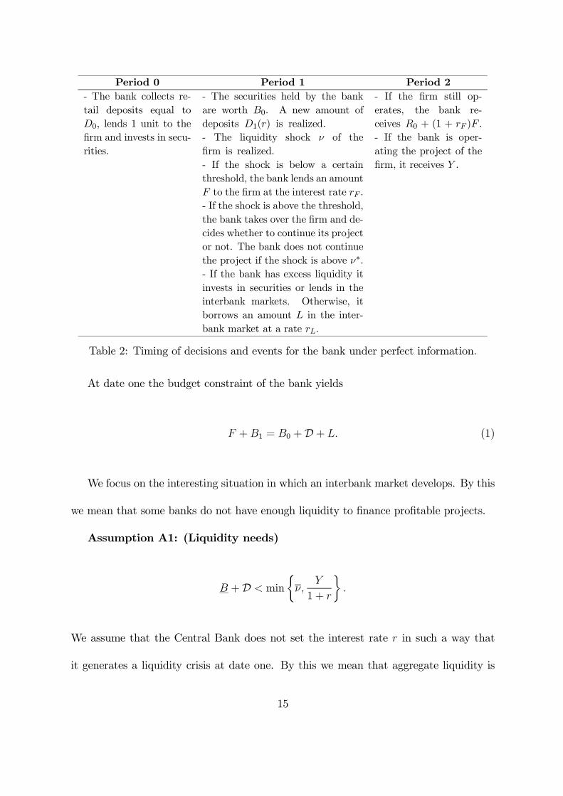
At date one the budget constraint of the bank yields

F +B1 = B0 +D + L. (1)

We focus on the interesting situation in which an interbank market develops. By this

we mean that some banks do not have enough liquidity to finance profitable projects.

Assumption A1: (Liquidity needs)

B +D < min

ν,

Y

1 + r

.

We assume that the Central Bank does not set the interest rate r in such a way that

it generates a liquidity crisis at date one. By this we mean that aggregate liquidity is

15

enough to serve the aggregate demand for bank deposits.

Assumption A2: (No liquidity crisis)

E [B0] +D ≥ 0.

2.3 The Firm - Bank Relationship

Recall that we are assuming that the bank has full information on the firm. We consider

the case in which, at date zero, the firm and the bank sign a credit line contract which

specifies the terms of the loan at date zero and the interest rate at date one. We assume

that, at date zero, the market for bank loans is competitive and this implies that the bank

loan rate at date one is set as equal to the interbank rate (rF = rL). We assume that the

interest rate on the date one bank loan that the firm demands is not renegotiable. We

consider explicitly the possibility that an individual bank is rationed in the interbank

market and we allow for an upper bound equal to L on interbank borrowing. The profit

function of the bank at date one depends on whether the firm defaults or not. When the

firm does not default, the problem of the bank is:

maxL,B1R0 + (1 + rL)F + (1 + r)B1 − (1 + γ)L−D1 (r)

s.t. (1) and L ≤ L.

(2)

When the firm defaults, then the bank appropriates the project, adds the assets of the

firm to its own portfolio, and chooses whether to continue or liquidate the project. If the

bank prefers to continue, its problem resembles the individual firm’s problem in section

16

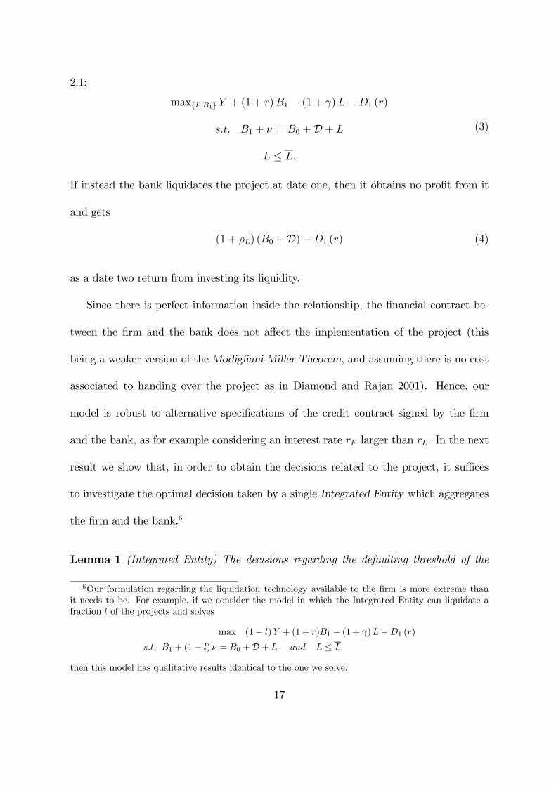
2.1:

maxL,B1 Y + (1 + r)B1 − (1 + γ)L−D1 (r)

s.t. B1 + ν = B0 +D + L

L ≤ L.

(3)

If instead the bank liquidates the project at date one, then it obtains no profit from it

and gets

(1 + ρL) (B0 +D)−D1 (r) (4)

as a date two return from investing its liquidity.

Since there is perfect information inside the relationship, the financial contract be-

tween the firm and the bank does not affect the implementation of the project (this

being a weaker version of the Modigliani-Miller Theorem, and assuming there is no cost

associated to handing over the project as in Diamond and Rajan 2001). Hence, our

model is robust to alternative specifications of the credit contract signed by the firm

and the bank, as for example considering an interest rate rF larger than rL. In the next

result we show that, in order to obtain the decisions related to the project, it suffices

to investigate the optimal decision taken by a single Integrated Entity which aggregates

the firm and the bank.6

Lemma 1 (Integrated Entity) The decisions regarding the defaulting threshold of the

6Our formulation regarding the liquidation technology available to the firm is more extreme thanit needs to be. For example, if we consider the model in which the Integrated Entity can liquidate afraction l of the projects and solves

max (1− l)Y + (1 + r)B1 − (1 + γ)L−D1 (r)

s.t. B1 + (1− l) ν = B0 +D + L and L ≤ L

then this model has qualitative results identical to the one we solve.

17

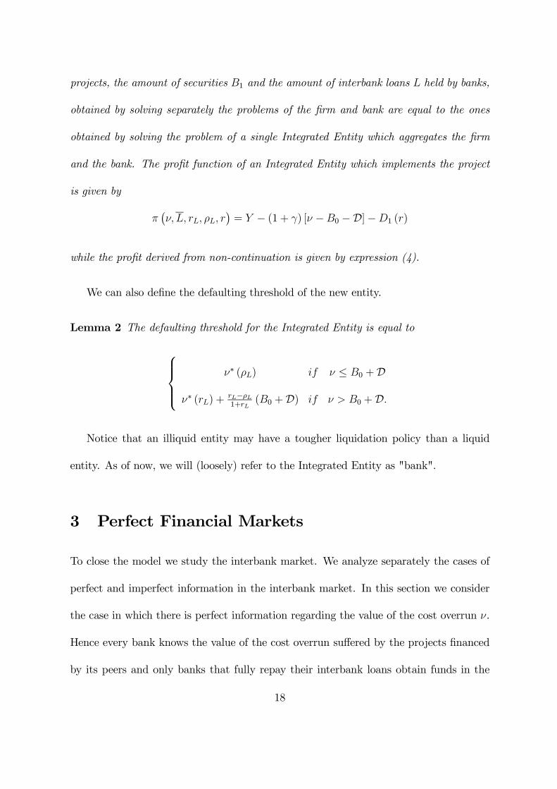
projects, the amount of securities B1 and the amount of interbank loans L held by banks,

obtained by solving separately the problems of the firm and bank are equal to the ones

obtained by solving the problem of a single Integrated Entity which aggregates the firm

and the bank. The profit function of an Integrated Entity which implements the project

is given by

π(ν, L, rL, ρL, r

)= Y − (1 + γ) [ν −B0 −D]−D1 (r)

while the profit derived from non-continuation is given by expression (4).

We can also define the defaulting threshold of the new entity.

Lemma 2 The defaulting threshold for the Integrated Entity is equal to

ν∗ (ρL) if ν ≤ B0 +D

ν∗ (rL) +rL−ρL1+rL

(B0 +D) if ν > B0 +D.

Notice that an illiquid entity may have a tougher liquidation policy than a liquid

entity. As of now, we will (loosely) refer to the Integrated Entity as "bank".

3 Perfect Financial Markets

To close the model we study the interbank market. We analyze separately the cases of

perfect and imperfect information in the interbank market. In this section we consider

the case in which there is perfect information regarding the value of the cost overrun ν.

Hence every bank knows the value of the cost overrun suffered by the projects financed

by its peers and only banks that fully repay their interbank loans obtain funds in the

18

interbank market. Hence, at date one, there is no risk premium and ρL = rL. Provided

that there is no liquidity shortage, then rL equals the risk free rate r. Hence the defaulting

threshold equals ν∗ (r), the closure decision is efficient and, as intuition suggests, it is

independent of the liquidity position (B0 +D) of an individual bank.7

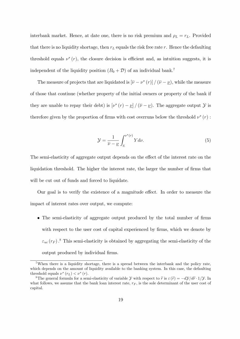
The measure of projects that are liquidated is [ν − ν∗ (r)] / (ν − ν), while the measure

of those that continue (whether property of the initial owners or property of the bank if

they are unable to repay their debt) is [ν∗ (r)− ν] / (ν − ν). The aggregate output Y is

therefore given by the proportion of firms with cost overruns below the threshold ν∗ (r) :

Y =1

ν − ν

∫ ν∗(r)

ν

Y dν. (5)

The semi-elasticity of aggregate output depends on the effect of the interest rate on the

liquidation threshold. The higher the interest rate, the larger the number of firms that

will be cut out of funds and forced to liquidate.

Our goal is to verify the existence of a magnitude effect. In order to measure the

impact of interest rates over output, we compute:

• The semi-elasticity of aggregate output produced by the total number of firms

with respect to the user cost of capital experienced by firms, which we denote by

εuc (rF ) .8 This semi-elasticity is obtained by aggregating the semi-elasticity of the

output produced by individual firms.

7When there is a liquidity shortage, there is a spread between the interbank and the policy rate,which depends on the amount of liquidity available to the banking system. In this case, the defaultingthreshold equals ν∗ (rL) < ν

∗ (r).8The general formula for a semi-elasticity of variable Y with respect to r is ε (r) = −dY/dr · 1/Y. In

what follows, we assume that the bank loan interest rate, rF , is the sole determinant of the user cost ofcapital.

19

• The semi-elasticity of aggregate output with respect to the interest rate set by the

Central Bank r, which we denote by εr (r).

The value of εr (r)− εuc (rF ) is a measure of the magnitude effect so that this effect

exists if and only if εr (r) > εuc (rF ).

In the perfect markets case, the user cost of capital equals the riskless interest rate

and εuc (rF ) equals εr (r).9 Using expression (5), the common semi-elasticity is easily

computed:

ε∗r (r) = ε∗uc (r) =ν∗ (r)

1 + r

1

ν∗ (r)− ν.

Thus, monetary policy affects aggregate output produced by firms through the interest

rate channel: larger interest rates shift the defaulting threshold ν∗ (r) and reduce the

measure of projects with positive net present value. This framework does not explain

the empirical facts because the magnitude effect is nonexistent.

The outcome obtained under perfect markets contrasts sharply with the outcome

obtained under the extreme case in which there is no interbank market. Under the

latter case, a bank suffering a liquidity shock larger than its liquidity holdings is unable

to continue its projects and is forced into default. Hence, when no interbank funding

is available, liquidity holdings determine the continuation of a project. In this set-up,

monetary policy is important because it affects the liquidity holdings of the banking

sector and interferes with continuation decisions. It is also worth pointing out that the

9Implicitly we are assuming that firms with a cost overrun ν ∈ ((Y −R0) /(1 + r), ν∗ (r)] are

restructured by the bank and continue. Hence their defaulting threshold equals ν∗ (r). Had weassumed that the firm is terminated and the bank takes over the project and we would have

Y =1/ (ν − ν) ·∫ (Y−R0)/(1+r)ν Y dν. The results that we obtain do not depend on this assumption.

20

assumptions of inelastic deposit supply to banks and borrowing firms being captured by

the bank are necessary but not sufficient conditions for the existence of liquidity effects

to occur. Under perfect markets, these assumptions do not prevent liquidity from being

channelled efficiently across banks, while they become relevant if the interbank market

is unable to perform an efficient allocation of funds.

4 Asymmetric Information

In this section we assume the existence of asymmetric information on the firm’s cost

overrun ν. This cost overrun is known to the firm and its financing bank that, because of

our assumption of relationship banking, has access to all relevant information. Obviously,

banks that have not established any relation with the firm, cannot observe the value taken

by ν, which is the source of asymmetric information.

The asymmetric information appears therefore in the interbank market in the con-

tractual relationship between a bank and its peers. We will assume that this asymmetry

allows insolvent banks to forbear and try to gamble for resurrection. Thus, as in Aghion,

Bolton, and Fries (1999) and Mitchell (2000) (where the accumulation of loan losses leads

the bank to hide them by renewing its bad loans in order to stay afloat), accumulated

loan losses produce a cascading effect here as well and triggers the bank’s gambling for

resurrection. In order to model gambling for resurrection in a simplified way, we assume

that bank managers have access to an alternative project at date one, which we refer

to as the private benefits project, that yields, at date two, a pledgeable return K lower

21

than Y, plus an amount of private benefits equal to ϑL.10 In order to make the results on

aggregate output directly comparable with the symmetric information case, we consider

K as an asset and not as new production of the alternative project. We assume that

depositors are senior with respect to interbank lenders and that D1 (r) ≤ K, so that

deposits are riskless. We interpret K −D1 (r) as the bank’s collateral in the unsecured

interbank market, that is the recovery value of interbank loans given default.

The interpretation for the private benefits project is akin to Calomiris and Kahn

(1991), in which managers have the opportunity to abscond with the funds and abscond-

ing is socially wasteful. We assume that 0 < ϑ < 2/3, which implies that, the larger the

amount of cash available to the bank manager, the larger its private benefit.11 Also, the

existence of moral hazard in the interbank market is in line with the findings by Ashcraft

and Bleakley (2006).

Given an equilibrium in the interbank market characterized by a maximum amount

of loan L, a bank manager can always secure a loan of size L, so that the value ϑL is its

reservation utility level. Thus, after observing its project cost overrun ν, the bank will

compare its profits level with the value of its private benefits, ϑL, and choose whether

to continue the project or to engage in the private benefits project. Obviously, since

this project yields K, any bank obtaining a loan with a repayment L(1+ rL) larger than

K − D1 (r), and choosing the private benefits project, will default. We refer to these

10Alternatively, it is possible, although analytically more involved, to assume that the final outcomeY is a random variable. This, jointly with limited liability, provides the option-like structure of stock-holders’ profits, which would obviously lead to the same results.

11When the variables Y and K are random, the assumption that private benefits depend on the sizeof the interbank loans is justified by the fact that, when a bank has a large amount of interbank loans,it is more likely to be rescued either by the authorities or by its peers.

22

banks as strategic defaulters. Remark, though, that the choice of strategical default is

endogenous and depends upon each bank’s liquidity position, given by ν, D and B0, as

well as on the interbank market interest rate rL.

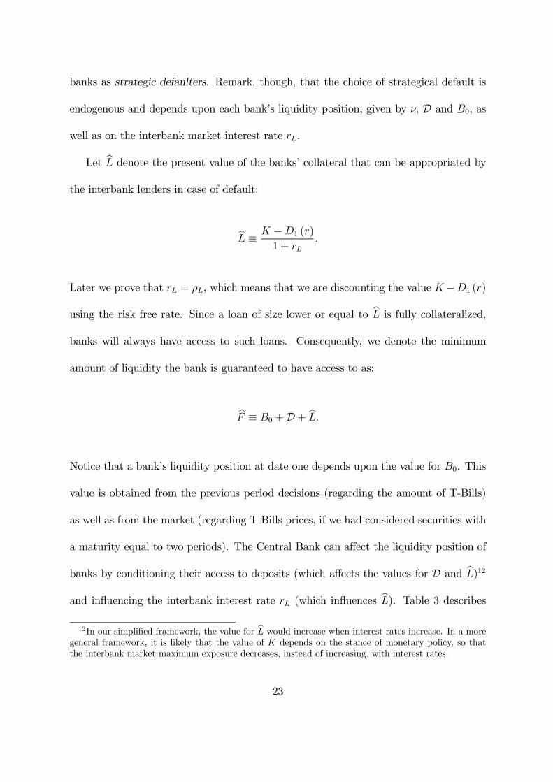
Let L denote the present value of the banks’ collateral that can be appropriated by

the interbank lenders in case of default:

L ≡K −D1 (r)

1 + rL.

Later we prove that rL = ρL, which means that we are discounting the value K −D1 (r)

using the risk free rate. Since a loan of size lower or equal to L is fully collateralized,

banks will always have access to such loans. Consequently, we denote the minimum

amount of liquidity the bank is guaranteed to have access to as:

F ≡ B0 +D + L.

Notice that a bank’s liquidity position at date one depends upon the value for B0. This

value is obtained from the previous period decisions (regarding the amount of T-Bills)

as well as from the market (regarding T-Bills prices, if we had considered securities with

a maturity equal to two periods). The Central Bank can affect the liquidity position of

banks by conditioning their access to deposits (which affects the values for D and L)12

and influencing the interbank interest rate rL (which influences L). Table 3 describes

12In our simplified framework, the value for L would increase when interest rates increase. In a moregeneral framework, it is likely that the value of K depends on the stance of monetary policy, so thatthe interbank market maximum exposure decreases, instead of increasing, with interest rates.

23

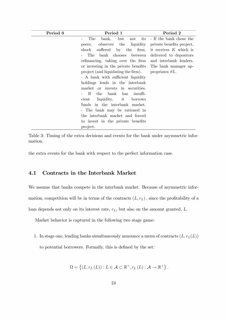
Period 0 Period 1 Period 2

- The bank, but not its

peers, observes the liquidity

shock suffered by the firm.

- The bank chooses between

refinancing, taking over the firm

or investing in the private benefits

project (and liquidating the firm).

- A bank with sufficient liquidity

holdings lends in the interbank

market or invests in securities.

- If the bank has insuffi-

cient liquidity, it borrows

funds in the interbank market.

- The bank may be rationed in

the interbank market and forced

to invest in the private benefits

project.

- If the bank chose the

private benefits project,

it receives K which is

delivered to depositors

and interbank lenders.

The bank manager ap-

propriates ϑL.

Table 3: Timing of the extra decisions and events for the bank under asymmetric infor-mation.

the extra events for the bank with respect to the perfect information case.

4.1 Contracts in the Interbank Market

We assume that banks compete in the interbank market. Because of asymmetric infor-

mation, competition will be in terms of the contracts (L, rL) , since the profitability of a

loan depends not only on its interest rate, rL, but also on the amount granted, L.

Market behavior is captured in the following two stage game:

1. In stage one, lending banks simultaneously announce a menu of contracts (L, rL(L))

to potential borrowers. Formally, this is defined by the set:

Ω =(L, rL (L)) : L ∈ A ⊂ R

+, rL (L) : A → R+.

24

2. In stage two, the borrowing banks decide to accept or not one of the contracts

offered by a specific bank. (For the sake of simplicity we suppose that, if they

are indifferent among the contracts offered by banks, then they randomize among

them).

A particular menu of contracts, the riskless competitive one, is particularly relevant

to characterize the interbank equilibrium. It is defined as follows:

Definition 1 The Riskless Competitive Contract Menu (RCCM) is defined as:

ΩP =(L, rL (L)) : L ∈

[0, L]

with rL = ρL

.

Under some assumptions, the RCCM characterizes the unique equilibrium set of

contracts. This implies that, despite lending being unsecured, there are no risk spreads

in the interbank market.13

4.2 Equilibrium Set of Contracts

The reason why, under some conditions, the equilibrium is restricted to the RCCM

class of riskless, zero profit contracts is quite intuitive. Agents with a low liquidity need

will always ask for a loan lower than L, which is riskless, and competition on any of

these contracts will lead to rL = ρL. Now, for contracts characterized by L > L, lenders

know that the behavior of strategic defaulters will be to ask for the largest possible loan.

13Yet, if the variable K were random, the concavity of the debt contract would yield a credit spreadfor interbank loans.

25

Because of this, any loan contract with L > L, will be dominated by a contract L − ε

as this slight reduction of the loan size attracts only non-defaulting banks, so that it is

always profitable. The difficulty is then to see whether deviations from the equilibrium

associated with the RCCM are possible, in which case no equilibrium would exist.14 We

impose conditions such that no contract outside the RCCM class makes positive profits.

The following assumptions allow us to focus on the case where a pure strategy equi-

librium with rationing in the interbank market exists. First, we disregard the case where

collateral is enough to guarantee a riskless interbank market, because this is equivalent

to reintroducing the perfect capital market we have already analyzed. This is why we

make the following assumption:

Assumption A3: (Rationing)

K + ϑK −D1 (r)

1 + r< Y.

In the same vein, we also want to discard the uninteresting case where banks have

enough liquidity to cope with any type of cost overrun. Assumption A4 implies that, at

least for large cost overruns, banks will have to borrow from the interbank market.

Assumption A4: (Liquidity needs’)

B +r

1 + rD1 (r)−D0 +

K

1 + r< min

ν,

Y

1 + r

.

14This non-existence may occur because banks compete both on prices and quantities, and changes inquantities affects credit risk. This is related to Stahl (1988) and Yannelle (1987) papers, where doubleBertrand competition may result in non-existence, and to Broecker (1990) where competition affectscredit risk, leading to the non-existence of pure strategies equilibrium.

26

Assumption A4 implies that F < min ν, Y/ (1 + r) for all banks, which means that

it is more restrictive than assumption A1.

The last assumption states that the adverse selection problem is not negligible.

Assumption A5: (Existence)

3

2

[Y −K − ϑK−D1(r)

1+r

1 + r

]≤ ν − E

[B0 +

K

1 + r+

r

1 + rD1 (r)−D0

].

The intuition for this assumption is as follows. The term inside the brackets in left

hand side of the above expression can be rewritten as

Y −D1 (r)− ϑK−D1(r)1+r

1 + r+ E [B0 +D]− E

[B0 +D +

K −D1 (r)

1 + r

]

which is the difference between what would be the "average" defaulting threshold without

rationing, that is[Y −D1 (r)− ϑL

]/ (1 + rL)+E [B0 +D] , and the "average" default-

ing threshold with rationing, E[B0 +D + L

], when the interbank rate equals r. Thus,

the left hand side of the expression in assumption A5 is a measure of the inefficiency

caused by rationing, while the right hand side is a proxy for the size of the mass of de-

faulters. Hence, assumption A5 guarantees that: (i) the mass of defaulters is sufficiently

large, so that lenders have no incentive to propose new contracts because the losses

associated to such contracts are larger than the potential gains; (ii) the inefficiencies

stemming from rationing and liquidation are not too large, as otherwise agents would

have strong incentives to propose deviating contracts.

Proposition 2 Under assumptions A2 to A5, the RCCM defines the unique equilibrium

27

set of contracts that exists in the interbank market. The defaulting threshold for the

Integrated Entity with liquidity B0 +D equals F .

It may be argued, based on Holmstrom and Tirole (1998) argument, that credit lines

play a key role in our model and that, consequently, restricting the class of contracts

available to banks to pure interbank contracts is quite a restrictive assumption. We

argue that, in fact, allowing for credit lines, would not change the equilibrium. This is

the case because banks will compete on the terms (initial fee, amount of the loan and

interest rate) of their credit lines. Prima facie, it seems indeed that the existence of a

credit line, allowing participants to obtain loans from their peers equal to an amount

L larger than L, would reduce the level of rationing and could improve efficiency. Yet,

such arrangement is vulnerable, ex post, to competition in the interbank market. Such

a credit line would entail financing strategic defaulters and, therefore, the initial fee

plus the interest rate will have to cover the cost of these negative net present value

loans. Consequently, a competing bank could offer a credit line with the same initial

fee and a loan slightly inferior to L at an interest rate substantially lower, as it will

not attract strategic defaulters. This strategy would separate all non-defaulting banks,

leaving strategic defaulters as the sole applicants to credit lines. Thus, competition

would reduce the amount of the credit line until the point where it will be identical to

the interbank loan itself and, hence, redundant.15

In the next section we characterize the equilibrium in the interbank market and we

15Consider the case in which banks have the possibility of extending irrevocable lines of credit at t = 0to their peers, in an amount larger than L, that can be used to meet liquidity needs at date 1. Providedthat the value of ν is sufficiently high, the mass of strategic defaulters imposes a burden on lenders suchthat, at least for banks with low levels of liquidity, credit lines are not profitable.

28

restrict our attention to the case in which there is rationing.16 When this happens, on

the one hand, banks with (relatively) more liquid balance sheets are able to finance the

liquidity needs of their clients, and firms dependent on these banks obtain finance as

long as they have projects with positive net present value. On the other hand, illiquid

banks are unable to shield their loan portfolio. Firms captive of these banks are unable

to obtain finance because they are being rationed and this entails the liquidation of

profitable projects.

5 Interbank Market Equilibrium and Monetary Pol-

icy

In order to study monetary transmission under asymmetric information in the interbank

market, we start by clarifying the equilibrium concept in our set-up.

The agents’ decision variables consist of their demand and supply of interbank loans

(L) and liquidity holdings (B1), and the equilibrium interest rate in the interbank market

(rL) is the one for which the aggregate excess demand for loans clears. Note that the

level of interest rates (r) is exogenously given.

In order to compute the equilibrium, we aggregate the individual net demands for

funds in the interbank market. We must have rL ≥ r, otherwise there is excess demand

in the market. When rL ≥ r, the individual net demand z for interbank funds by a bank

16In a dynamic model, we could think of several regimes where assumption A4 is relaxed, so that insome regimes rationing is negligible as banks have enough liquidity, while in other regimes rationing is akey characteristic of the interbank market. This would allow to understand the way interbank lendingmay suddenly dry out. Because we want to illustrate rationing we will dispense with a multiregimeanalysis and assume A4 holds in our static model.

29

with cost ν and liquidity B0 is

z =

ν +B1 (B0, ν)−B0 −D if ν ≤ B0 +D

ν −B0 −D if B0 +D < ν ≤ F

L if ν ≥ F

where B1 (B0, ν) denotes the holdings of treasuries, at the end of date one, by a bank

which inherits B0 and suffers a liquidity shock ν. When rL = r we have B1 (B0, ν) ∈

[0,∞) and when rL > r we have B1 (B0, ν) = 0 for all banks. The aggregate net demand

for funds in the interbank market, Z, is the sum of (positive and negative) individual

excess demands for loans.

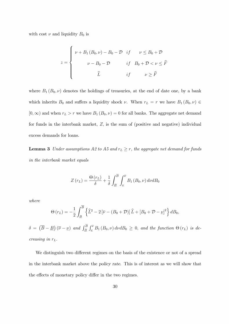
Lemma 3 Under assumptions A2 to A5 and rL ≥ r, the aggregate net demand for funds

in the interbank market equals

Z (rL) =Θ (rL)

δ+1

δ

∫ B

B

∫ ν

ν

B1 (B0, ν) dνdB0

where

Θ(rL) = −1

2

∫ B

B

L2 − 2 [ν − (B0 +D)] L+ [B0 +D − ν]

2dB0,

δ =(B −B

)(ν − ν) and

∫ BB

∫ ννB1 (B0, ν) dνdB0 ≥ 0, and the function Θ(rL) is de-

creasing in rL.

We distinguish two different regimes on the basis of the existence or not of a spread

in the interbank market above the policy rate. This is of interest as we will show that

the effects of monetary policy differ in the two regimes.

30

• An excess liquidity regime occurs if there is no spread in the interbank market,

that is rL = r. This will be the case if any bank holds a positive amount of T-Bills

in equilibrium, that is B1 (B0, ν) > 0.

• A liquidity shortage regime occurs if there is a positive spread between the inter-

bank market return rL and the target rate r, that is rL > r. In this case, it is not

profitable for any bank to hold T-Bills, and B1 (B0, ν) = 0.

The two regimes can be distinguished according to the value taken by Θ(r) , which

is a proxy for the value of the aggregate net demand for funds when B1 (B0, ν) = 0 for

all banks. If Θ(r) > 0, then the economy is in the liquidity shortage regime; if instead

Θ(r) ≤ 0, the economy is in the excess liquidity regime.

Lemma 3 allows to clarify the link between the amount of aggregate liquidity shocks

(i.e. cost overruns) and the liquidity regime. For the economy to be in the excess liquid-

ity regime, expressionL2 − 2 [ν − (B0 +D)] L+ [B0 +D − ν]

2must be positive on

average. This will be the case when (B0 +D) , the liquidity position of banks is large,

so that the term [ν − (B0 +D)] is small, while the term [B0 +D − ν] is large. In other

terms, the occurrence of an excess liquidity regime, as well as the occurrence of a liq-

uidity shortage one, will depend upon the position of (B0 +D) within the [ν, ν] interval.

This is quite intuitive, as we have assumed a uniform distribution for ν, (B0 +D) rep-

resents the banks’ liquidity supply and the (feasible) liquidity demand is driven by the

extent of the liquidity shocks that are distributed in the [ν, ν] . Of course, the amount of

collateral determining L will also affect the aggregate economic regime, as it determines

the maximum amount of a feasible interbank loan.

31

Proposition 3 (Equilibrium in the Interbank Market) Under asymmetric information

and assumptions A2 to A5, there exists a unique equilibrium in the interbank market,

characterized by rL = ρL. In the excess liquidity regime, we obtain rL = r, while in the

liquidity shortage regime the interbank market rate is given by:

rL =K −D1 (r)

(ν −E [B0]−D)−√(ν − E [B0]−D)

2 −[σ2B0 + (E [B0] +D − ν)

2] − 1.

Market clearing pins down the interbank rate, which represents the opportunity cost

of funds for interbank lenders. As intuition suggests, the interbank rate equals r as long

as the liquidity available in the interbank market is large enough. Otherwise liquidity is

scarce and there is a spread between the interbank rate and the T-Bills rate that is purely

liquidity driven, as interbank loans are effectively fully collateralized. The arbitrage

between the interbank market and the T-Bill market does not operate because T-Bills

are in the hands of consumers and not in those of the banks. The lack of liquidity that

creates the wedge between the T-Bills rate and the interbank rate has real implications

on firms’ access to credit, as the fringe of firms with a cost overrun ν in the interval

(F (rL), F (r)

)will be liquidated.

Notice that, as intuition suggests, the spread increases when the demand for liquidity

increases, that is, for instance, when the value of collateral K −D1 (r) increases. More

interesting is the observation that a higher dispersion of T-Bills across banks, σB0 , implies

a lower interbank market rate. This happens because a larger dispersion implies the

existence of both more agents with excess liquidity and more rationed agents, generating

32

an aggregate liquidity supply.

It is useful to note that, in the liquidity excess case, F is independent of the interbank

market rate which is equal to the T-Bills rate so that, for any r, we have a corresponding

F . In the liquidity shortage case, the values for F and rL are jointly determined in

equilibrium.

6 Implications Regarding the Main Empirical Facts

The object of this section is to analyze to what extent our results fit in with the existing

empirical findings.

6.1 Two Empirical Effects

In order to evaluate the effects of monetary policy we assess the effects of a shift in the

policy rate r. Recall that rF = rL = ρL.

Proposition 4 (Magnitude Effect) Under asymmetric information and assumptions A2

to A5, the aggregate effect of an interest rate shock is larger than the aggregate of indi-

vidual effects of an increase in the user cost of capital.

The magnitude effect is positive because εr (r) > 0 while εuc (rF ) = 0. The semi-

elasticity with respect to the user cost of capital is null because rationed firms are insen-

sitive to the user cost of capital (while, in the perfect markets case, the continuation of a

project is mainly determined by the interest rate on bank credit). In our framework, the

magnitude effect hinges on the fact that the banking system (and not firms) determines

33

endogenously the marginal projects that are undertaken in the economy. Firms take the

threshold F as exogenous and, because of asymmetric information, projects with cost

overruns above F are liquidated. Consequently, for these projects, the opportunity cost

of funds is not rF = rL, but the shadow price of the credit constraint.

Recall that the defaulting threshold, for a rationed entity holding an amount B0

in securities, equals F = B0 + [D1 (r)−D0] + [K −D1 (r)] / (1 + rL). This threshold

reflects the availability of funds to the banking system and is influenced by monetary

policy through two channels: (i) the balance sheet channel because monetary policy

affects the present value of collateral K − D1 (r); (ii) the deposit base of the banking

system D1 (r). Hence, when monetary policy is tightened, the value for F declines,

through the combination of these two effects, making the credit rationing constraint

more severe with a higher number of projects being liquidated.

When there is a liquidity shortage, we must add, on top of the rationing channel, a

spread - augmented interest rate channel similar to the one described by Stein (1998).

Depending on the effect of policy rates on the interbank rate spread, that is depending on

whether drL/dr is larger or inferior to one, the spread - augmented interest rate channel

can amplify or mitigate the rationing channel.

Notice that we proceed to compare, within a given set-up, the semi-elasticity of the

aggregate output with respect to the policy rate with the semi-elasticity with respect to

the user cost of capital. The result is that themagnitude effect occurs as a consequence of

asymmetric information and the resulting rationing in the credit market. As established

in Section 3, no similar result holds in a perfect information set-up. A completely different

34

exercise would be to compare the elasticities across different set-ups. This would show

how asymmetric information increases the semi-elasticities of output with respect to

interest rates, but this would not be related in any way to the magnitude effect.17

To conclude this section, it is worth exploring the connection between our theoretical

model and the empirical results obtained by Kashyap and Stein (2000). They document

that the impact of monetary policy on the lending behavior of banks is more pronounced

for banks with less liquid balance sheets, where liquidity is measured by the absolute

amount of liquid securities that the bank holds. Because of the construction of our

model, it is not surprising that we obtain a result with the same flavour.

Proposition 5 (Kashyap and Stein Liquidity Effect) Under asymmetric information

and assumptions A2 to A5, the impact of shifts in the interest rate r on the supply of

credit to firms is larger for banks with a smaller amount of T-Bills (B0).

Because our model is based on the existence of an imperfection in the interbank

market that prevents perfect circulation of reserves from one bank to another, the result

is not surprising. The previous proposition asserts the consistency of our framework

to cope with the issues documented by Kashyap and Stein (2000). Kashyap and Stein

(2000) argue that their result is entirely driven by the smaller banks, which are those

that are more affected by asymmetric information problems. We do not explore the

differences in access to liquidity by large and small banks, because we assume that all

17The effect would rather be connected with the financial accelerator obtained in related models (seeBernanke and Gertler 1989, 1990).

35

banks have the same size. Note, however, that asymmetric information is the main factor

responsible for the results in proposition 5.

Our approach based on the existence of an imperfection in the interbank market seems

to be consistent with other empirical results. Indeed, if our framework is the correct one,

banks having access to sources of reserves other than the interbank market, such as an

internal capital market, should not react as much to shifts in interest rates. This is

confirmed by the Ashcraft (2006)’s empirical analysis, who reports that loan growth of

banks affiliated with multi-bank holding companies is much less sensitive to changes in

the federal funds rate. Additionally, Ehrmann andWorms (2004) argue that the Kashyap

and Stein liquidity effect does not hold for the German banking system because small

banks access the interbank market indirectly through the large head institutions of their

respective network organizations, and the interbank flows within these networks allow

banks to insulate their loan portfolio from monetary shocks.

Our model allows for a discussion of the composition effect.18 As it is, our model does

not distinguish between different maturities in the portfolio of loans, as there is a unique

representative project facing a unique representative bank. Still, the extension to a well

diversified portfolio of loans is straightforward and, a bank without sufficient liquidity to

finance the cost overruns of its clients, will have to ration their clients regardless of the

maturity of their investments. Additionally, it is likely that long term interbank loans

are more severely affected by asymmetric information and rationing problems. As long

18It has been suggested that this effect is already well understood since, when the central bank raisesshort-term rates, it is also signaling the stance of monetary policy in the medium-term, thus affectingmedium-run investment decisions. Yet, in can be argued that the ability of the central bank to influencelong-term rates is negligible and, therefore, its decisions should have an insignificant effect on residentialinvestment.

36

as portfolio management strategies followed by banks prescribe matching the maturities

of their assets and liabilities, it is likely that the mechanisms described apply mainly to

long term lending and monetary policy affects mostly bank loans with a larger maturity.

6.2 Financial Structure and Monetary Policy Transmission

Although our model is based on a number of restrictive assumptions, the main argument

is quite intuitive and it is expected to carry out in more general frameworks. The

rationing channel will affect a larger number of firms, the larger the degree of asymmetric

information, the higher the interbank credit risk and the stronger the level of relationship

banking. To verify the possible empirical predictions, we associate these characteristics

of our model to variables that can be observed. We claim that asymmetric information

is related to a lower level of development for financial markets and the importance of

small banks. Also, the existence of credit risk in the interbank market can be measured

by an index of bank health and the strong relationships that makes it too costly for

firms in our model to switch from one bank to another implies, by assumption, a strong

dependence on bank loans, which is related with the availability of alternative forms of

finance.

Although testing our predictions is outside the scope of our contribution, it is interest-

ing to relate our results with the ones obtained by Kashyap and Stein (1997), Cecchetti

(1999) and Mihov (2001) that make similar points. Cecchetti (1999) builds indices on

three key credit-channel factors, and uses these indices to build a summary statistic for

the "Predicted Effectiveness of Monetary Policy". The definition of the summary statis-

37

0

0,5

1

1,5

2

2,5

3

0 1 2 3 4 5 6 7

Predicted Efectiveness of Monetary Policy

Cu

mu

lati

ve

De

via

tio

n o

f O

utp

ut

fro

m T

ren

d

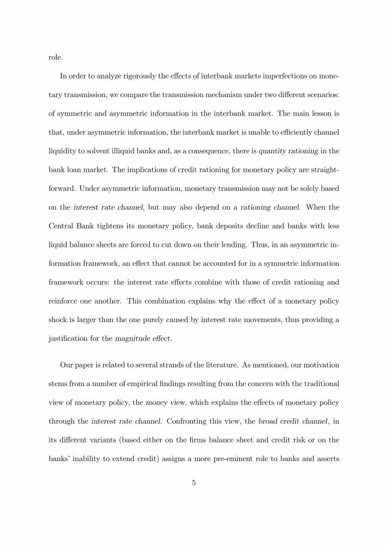
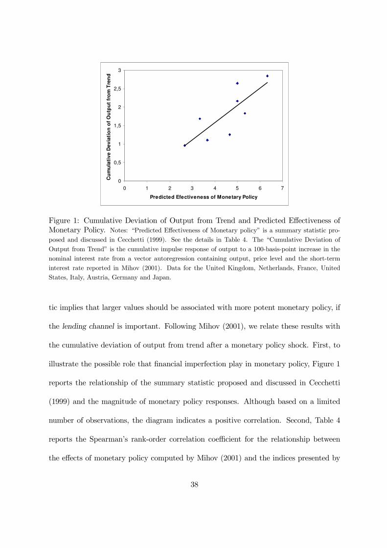
Figure 1: Cumulative Deviation of Output from Trend and Predicted Effectiveness ofMonetary Policy. Notes: “Predicted Effectiveness of Monetary policy” is a summary statistic pro-

posed and discussed in Cecchetti (1999). See the details in Table 4. The “Cumulative Deviation of

Output from Trend” is the cumulative impulse response of output to a 100-basis-point increase in the

nominal interest rate from a vector autoregression containing output, price level and the short-term

interest rate reported in Mihov (2001). Data for the United Kingdom, Netherlands, France, United

States, Italy, Austria, Germany and Japan.

tic implies that larger values should be associated with more potent monetary policy, if

the lending channel is important. Following Mihov (2001), we relate these results with

the cumulative deviation of output from trend after a monetary policy shock. First, to

illustrate the possible role that financial imperfection play in monetary policy, Figure 1

reports the relationship of the summary statistic proposed and discussed in Cecchetti

(1999) and the magnitude of monetary policy responses. Although based on a limited

number of observations, the diagram indicates a positive correlation. Second, Table 4

reports the Spearman’s rank-order correlation coefficient for the relationship between

the effects of monetary policy computed by Mihov (2001) and the indices presented by

38

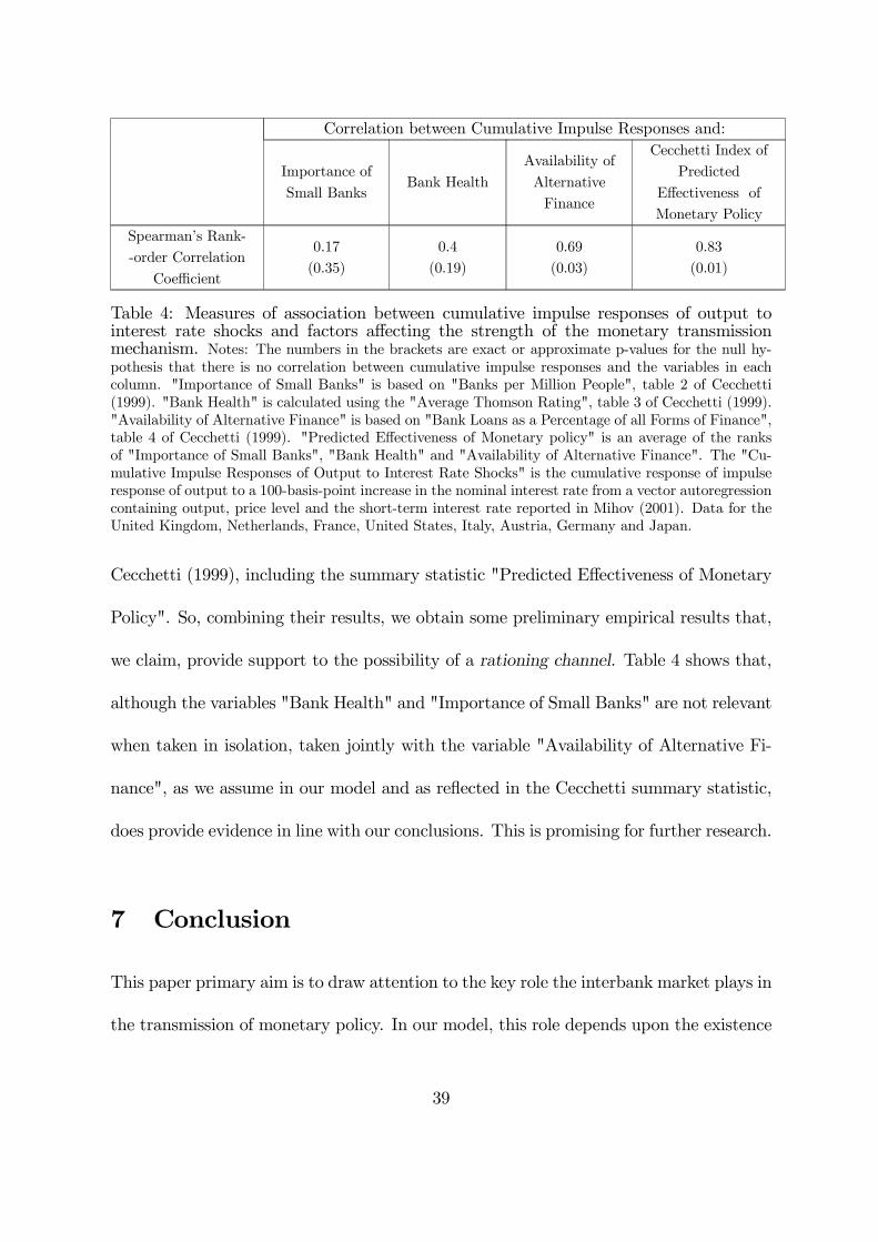
Correlation between Cumulative Impulse Responses and:

Importance of

Small BanksBank Health

Availability of

Alternative

Finance

Cecchetti Index of

Predicted

Effectiveness of

Monetary Policy

Spearman’s Rank-

-order Correlation

Coefficient

0.17

(0.35)

0.4

(0.19)

0.69

(0.03)

0.83

(0.01)

Table 4: Measures of association between cumulative impulse responses of output tointerest rate shocks and factors affecting the strength of the monetary transmissionmechanism. Notes: The numbers in the brackets are exact or approximate p-values for the null hy-pothesis that there is no correlation between cumulative impulse responses and the variables in eachcolumn. "Importance of Small Banks" is based on "Banks per Million People", table 2 of Cecchetti(1999). "Bank Health" is calculated using the "Average Thomson Rating", table 3 of Cecchetti (1999)."Availability of Alternative Finance" is based on "Bank Loans as a Percentage of all Forms of Finance",table 4 of Cecchetti (1999). "Predicted Effectiveness of Monetary policy" is an average of the ranksof "Importance of Small Banks", "Bank Health" and "Availability of Alternative Finance". The "Cu-mulative Impulse Responses of Output to Interest Rate Shocks" is the cumulative response of impulseresponse of output to a 100-basis-point increase in the nominal interest rate from a vector autoregressioncontaining output, price level and the short-term interest rate reported in Mihov (2001). Data for theUnited Kingdom, Netherlands, France, United States, Italy, Austria, Germany and Japan.

Cecchetti (1999), including the summary statistic "Predicted Effectiveness of Monetary

Policy". So, combining their results, we obtain some preliminary empirical results that,

we claim, provide support to the possibility of a rationing channel. Table 4 shows that,

although the variables "Bank Health" and "Importance of Small Banks" are not relevant

when taken in isolation, taken jointly with the variable "Availability of Alternative Fi-

nance", as we assume in our model and as reflected in the Cecchetti summary statistic,

does provide evidence in line with our conclusions. This is promising for further research.

7 Conclusion

This paper primary aim is to draw attention to the key role the interbank market plays in

the transmission of monetary policy. In our model, this role depends upon the existence

39

of heterogeneous liquidity shocks for banks facing asymmetric information. In this way

we explain how financial imperfections may account for some empirical facts regarding

the transmission mechanism of monetary policy. First, asymmetric information in the

interbankmarket can generate rationing and helps justifying the liquidity effect presented

by Kashyap and Stein (2000). Second, financial imperfections justify the existence of a

magnitude effect because rationing creates a wedge between the shadow price of funds

and the interest rate in the economy. Because banks themselves are rationed, there is

no interest rate the borrowing firms can offer to entice banks into increasing their credit

supply. Consequently, these firms that are bound to be liquidated do not appear as part

of the demand for funds.

We have considered a very restrictive function explaining the behavior of retail de-

posits. Alternatively, we could think that the amount of retail deposits collected by an

individual bank is partially determined by the interest rate quoted by the bank. There

is no reason to think that our results would change significantly if we allowed for this

possibility. The value of collateral, K, effectively sets an upper bound for the overall

funding by the bank implying that a larger amount of deposits collected by a bank would

be exactly offset by a corresponding decrease in interbank borrowing, so that banks will

not be interested in increasing deposit interest rates, as the elasticity is low and it implies

an equivalent decrease in interbank market funding. So, it will only be profitable at the

margin to adjust deposit interest rates and increase the deposit supply.

Apart from considering explicitly short term and long term lending among banks,

our model is open to broader interpretations. It would be straightforward to extend our

40

set-up to the case in which banks have access to alternative sources of finance, such as

certificates of deposit. In this case, the set-up in our model would be closely related

to Stein (1998)’s but, while he focuses on a separating equilibrium in the market for

unsecured forms of finance (highlighting the role of the spread - augmented interest rate

channel), we focus on a pooling equilibrium characterized by rationing.

Although we have focused on the rationing channel, our model can easily accommo-

date other channels. For example, when there is a shortage of liquidity in the interbank

market, equilibrium is characterized by a positive spread between the interbank market

and the T-Bills rate, and monetary policy has the ability to influence the size of the

spread. In this case, we obtain a channel very similar to Stein (1998). Finally, our

model has relevant empirical implications regarding future research on the determinants

of business investment and bank loan behavior.

References

[1] Ackerloff, George. (1970) "The Market for Lemons: Quality Uncertainty and the

Market Mechanism." Quarterly Journal of Economics, 84, 488-500.

[2] Aghion, Philippe, Patrick Bolton, and Steven Fries. (1999) "Optimal Design of

Bank Bailouts: The Case of Transition Economies." Journal of Institutional and

Theoretical Economics, 155:1, 51-70.

[3] Angeloni, Ignazio, Benoît Mojon, Anil K. Kashyap, and Daniele Terlizzese. (2002)

"Monetary Transmission in the Euro Area : Where Do We Stand?" European Cen-

41

tral Bank Working Paper, 114, European Central Bank.

[4] Ashcraft, Adam B.. (2006) "New Evidence on the Lending Channel." Journal of

Money, Credit, and Banking, 38:3, 751-775.

[5] Ashcraft, Adam B., and Hoyt Bleakley. (2006) "On the Market Discipline of In-

formationally Opaque Firms: Evidence from Bank Borrowers in the Federal Funds

Market." Staff Reports of the Federal Reserve Bank of New York, 257, Federal

Reserve Bank of New York.

[6] Bhattacharia, Sudipto, and Douglas Gale. (1987) "Preference Shocks, Liquidity, and

Central Bank Policy." In New Approaches to Monetary Economics, edited by W.

Barnett and K. Singleton, pp. 69-88. Cambridge: Cambridge University Press.

[7] Berger, Allen, and Gregory Udell. (1992) "Some Evidence on the Empirical Signifi-

cance of Credit Rationing." Journal of Political Economy, 100:5, 1047-1077.

[8] Bernanke, Ben, and Mark Gertler. (1989) "Agency Costs, Net Worth, and Business

Fluctuations." American Economic Review, 79:1, 14-31.

[9] Bernanke, Ben, and Mark Gertler. (1990) "Financial Fragility and Economic Per-

formance." Quarterly Journal of Economics, 105:1, 87-114.

[10] Bernanke, Ben, and Mark Gertler. (1995) "Inside the Black Box: The Credit Chan-

nel of Monetary Policy Transmission." Journal of Economic Perspectives, 9:4, 27-48.

[11] Boot, Arnoud. (2000) "Relationship Banking: What Do We Know?" Journal of

Financial Intermediation, 9:1, 7-25.

42

[12] Broecker, Thorsten. (1990) "Credit-Worthiness Tests and Interbank Competition."

Econometrica, 58:2, 429-52.

[13] Calomiris, Charles W., and Charles M. Kahn. (1991) "The Role of Demandable

Debt in Structuring Optimal Banking Arrangements." American Economic Review,

81, 497-513.

[14] Cecchetti, Stephen. (1999) "Legal Structure, Financial Structure, and the Monetary

Policy Transmission Mechanism." Federal Reserve Bank of New York Economic

Policy Review, July 1999, 9-28.

[15] Cleary, Sean. (1999) "The Relationship Between Firm Investment and Financial

Status." Journal of Finance, 54, 673-692.

[16] Cocco, Joao F., Francisco J. Gomes, and Nuno C. Martins. (2003) "Lending Rela-

tionships in the Interbank Market." AFA 2004 San Diego Meetings.

[17] Degryse, Hans, and Steven Ongena. (2005) "Distance, Lending Relationships, and

Competition." Journal of Finance, 60:1, 231-266.

[18] Diamond, Douglas W., and Raghuram G. Rajan. (2001) "Liquidity Risk, Liquid-

ity Creation and Financial Fragility: A Theory of Banking." Journal of Political

Economy 109:2, 287-327.

[19] Ehrmann, Michael, and Andreas Worms. (2004) "Bank Networks and Monetary

Policy Transmission." Journal of the European Economic Association, 2:6, 1148-

1171.

43

[20] Flannery, Mark. (1996) "Financial Crisis, Payment System Problems, and Discount

Window Lending." Journal of Money, Credit, and Banking, 28:4, 804-24.

[21] Freixas, Xavier, and Cornelia Holthausen. (2005) "Interbank Market Integration

under Asymmetric Information." Review of Financial Studies, 18:2, 459-490.

[22] Furfine, Craig. (1999) "The Microstructure of the Federal Funds Market." Financial

Markets, Institutions and Instruments, 8, 24-44.

[23] Furfine, Craig. (2001) "Banks Monitoring Banks: Evidence from the Overnight

Federal Funds Market." Journal of Business, 74:1, 33-58.

[24] Goodfriend, Marvin, and Robert King. (1988). " Financial Deregulation, Monetary

Policy, and Central Banking." Federal Reserve Bank of Richmond Economic Review,

May/June 1988, 3-22.

[25] Holmstrom, Bengt, and Jean Tirole. (1998) "Private and Public Supply of Liquid-

ity." Journal of Political Economy, 106:1, 1-40.

[26] Hubbard, R. Glenn. (1998) "Capital Market Imperfections and Investment." Journal

of Economic Literature, 35, 193-225.

[27] Kaplan, Steven K., and Luigi Zingales. (1997) "Do Investment Cash Flow Sensi-

tivities Provide Useful Measures of Financing Constraints?" Quarterly Journal of

Economics, 112, 169-215.

44

[28] Kashyap, Anil K., and Jeremy Stein. (1994) "Monetary Policy and Bank Lending."

InMonetary Policy, edited by N. Gregory Mankiw, pp. 221-56. Chicago: University

of Chicago Press.

[29] Kashyap, Anil K., and Jeremy Stein. (1997) "The Role of Banks in Monetary Pol-

icy: a Survey with Implications for the EMU." Federal Reserve Bank of Chicago

Economic Perspectives, September 1997, 8-18.

[30] Kashyap, Anil K., and Jeremy Stein. (2000) "What Do a Million Observations

on Banks Have to Say About the Transmission of Monetary Policy?". American

Economic Review, 90, 407-28.

[31] Kashyap, Anil K., Jeremy C. Stein and David W. Wilcox. (1993) "Monetary Pol-

icy and Credit Conditions: Evidence From the Composition of External Finance"

American Economic Review, 83, 78-98.

[32] Mihov, Ilian. (2001) "Monetary Policy Implementation and Transmission in the

European Monetary Union." Economic Policy, 33, 370-406.

[33] Mitchell, Janet. (2000) "Bad Debts and the Cleaning, Tranferring of Banks’ Balance

Sheets: An application to Transition Economies." Journal of Financial Intermedia-

tion, 10:1, 1-27.

[34] Rochet, Jean-Charles, and Jean Tirole. (1996) "Interbank Lending and Systemic

Risk." Journal of Money, Credit, and Banking, 28:4, 733-62.

45

[35] Schiantarelli, Fabio. (1995) "Financial Constraints and Investment: a Critical Re-

view of Methodological Issues and International Evidence." In Is bank lending im-

portant for the transmission of Monetary Policy?, edited by Joe Peek and Eric S.

Rosengren, pp. 177-214, Boston: Federal Reserve Bank of Boston.

[36] Schwartz, Anna. (1992) "The Misuse of the Fed’s Discount Window." Federal Re-

serve of St. Louis Review, September/October 1992, 58-69.

[37] Stahl, Dale O.. (1988) "Bertrand Competition for Inputs and Walrasian Outcomes."

American Economic Review, 78, 189-201.

[38] Stein, Jeremy. (1998) "An Adverse-Selection Model of Bank Asset and Liability

Management with Implications for the Transmission of Monetary Policy." RAND

Journal of Economics, 29:3, 466-486.

[39] Stiglitz, Joseph E., and Andrew Weiss. (1981) "Credit Rationing in Markets with

Imperfect Information." American Economic Review, 71, 393-410.

[40] Van den Heuvel, Skander. (2006) "The Bank Capital Channel of Monetary Policy."

Society for Economic Dynamics 2006 Meeting Papers, 512.

[41] Yannelle, Marie-Odile. (1997) "Banking Competition and Market Efficiency." Re-

view of Economic Studies, 64, 215-239.

46

A Appendix

A.1 Proof of Lemma 1

Let

Λ ≡ Λ (r,B0) ≡ B0 +D.

The profit function of an entity that integrates the firm and the bank is obtained by

aggregating the profits of the firm and bank and considering the restrictions of both

entities. The problem of the Integrated Entity is

maxL,B1 Y + (1 + r)B1 − (1 + γ)L−D1 (r)

s.t. B1 + ν = Λ+ L

L ≤ L.

(6)

We compare the solution to problem (6) with the solutions obtained with independent

entities. There are two cases that we must consider.

In the first case, ν ≤ minΛ + L, ν∗ (rL)−

R01+rL

and the firm borrows ν and does

not default. The profit of the firm equals ΠF = Y −R0− (1 + rL) ν and the bank solves

problem (2) with F = ν.

• If γ > r then B1 = 0 and, if the bank continues its activity, its profit equals

ΠB = R0+(1 + γ) Λ−D1 (r) and it satisfies the loan demand by the firm and sets

L = ν − Λ ≤ L. If the bank strategically defaults, it obtains (1 + ρL) Λ −D1 (r).

Comparing both alternatives implies that the bank prefers to continue its activity

because R0 > 0.

47

• If γ = r then B1 ≥ 0. Banks do not borrow interbank funds to invest in treasuries.

If the bank continues its activity, its profit equals ΠB = R0 + (1 + γ) Λ − D1 (r)

and it satisfies the loan demand by the firm. The bank sets L = ν−Λ when ν ≥ Λ

or L = 0 and B1 = Λ − ν if Λ > ν. If the bank strategically defaults, it obtains

(1 + ρL) Λ−D1 (r). Comparing both alternatives implies that the bank prefers to

continue its activity because R0 > 0.

We compare these results with the ones obtained by solving the problem from the

Integrated Entity. If we solve problem (6), and take into account that the restriction

L ≤ L does not bind, the profit from the Integrated Entity equals ΠF+ΠB which is larger

than the payoff derived from strategic default. Hence the Integrated Entity continues

the project. It uses the same decision rules as individual banks regarding the amounts

of interbank loans L and treasuries B1.

In the second case ν > minΛ + L, ν∗ (rL)−

R01+rL

. The firm defaults and the bank

appropriates the project. In this case the profit of the bank is given by the solution to

problem (3) which is the profit of an Integrated Entity.

A.2 Proof of Lemma 2

The profit from continuation is πcont = Y − (1 + γ) ν − Λ − D1 (r) , while the profit

from liquidation is πliq = (1 + ρL) Λ −D1 (r) . The bank’s threshold will be the one for

which ∆π = πcont − πliq equals zero.

When ν ≤ Λ, then γ = ρL and ∆π = 0 implies Y = (1− ρL) ν, so that the defaulting

threshold equals ν∗ (ρL).

48

When ν > Λ, then the Integrated Entity is a borrower and the defaulting threshold

equals ν∗ (rL) +rL−ρL1+rL

Λ .

A.3 Proof of Proposition 2

We use the concept of Subgame Perfect Nash Equilibrium (SPNE). We begin by the

last stage of the game.

Remark 1 Defaulting borrowers pool on the contract that grants the largest loan.

Remark 2 In every SPNE lenders must earn exactly zero expected profits on every

equilibrium contract.

The former remark is obvious. Regarding the latter, note that the situation is akin

to the standard Bertrand competition situation so that, if a contract makes profit, there

is an incentive for competitors to undercut the interest rates and obtain a larger share

of the market. Let

κ ≡ K −D1 (r) .

Lemma 4 In any SPNE lenders must set rL = ρL and L ≤ L on every equilibrium

contract.

Proof. Suppose that there is an SPNE for which a measure of µ borrowers apply for

a loan L at a rate rL > ρL. Given remark 2 the expected profits made on this contract

are null and two cases are possible:

• In the first case, L > κ1+ρL

and there is a counterpart risk premium and some

non defaulters signing the contract pay a premium because of strategic defaulters

49

buying the contract. Then one of the lenders can offer a contract with a loan L−ε

and interest rate rL−ε′, with 0 < ε < L− κ

1+ρLand 0 < ε′ < rL−ρL, that attracts

all (nondefaulting) borrowers with κ1+ρL

< ν < L − ε. The profits made on this

contract are positive since ρL < rL − ε′. Hence ρL ≥ rL, but since ρL > rL is not

possible we must have rL = ρL.

• In the second case, L ≤ κ1+ρL

and there is no risk and remark 2 implies rL = ρL.

We now prove that the maximum loan available in the interbank market equals L.

To see this, suppose that the maximum loan was L, with L > L. Then it must be the

case that all strategic defaulters choose L. Given that rL = ρL then there is a lender

making losses in equilibrium and this contradicts remark 2: we must therefore have a

maximum loan L such that L ≤ L. But if L < L, then one of the lending banks can

earn positive profits by offering a contract with a loan L ∈(L, L

]with rL > ρL which

contradicts remark 2. Hence the maximum loan available in the interbank market equals

L.

Lemma 5 Nondefaulting borrowers with ν − Λ ≤ L receive a loan equal to ν − Λ.

Proof. Obviously if a nondefaulting borrower was rationed, a deviating bank could

offer her a loan and make positive profits. The possibility of a borrower asking for a loan

larger than ν − Λ is ruled out by the assumption that agents do not borrow from the

interbank market to invest in T-Bills when r ≤ ρL.

Lemma 6 Defaulting borrowers sign a contract with a loan equal to L at an interest

rate rL = ρL.

50

Proof. This result is implied by Lemma 4 and the assumption that ϑ > 0.

So far we have proved that the RCCM characterizes the only possible equilibrium.

We now prove that equilibrium is characterized by rationing. For this we use assumption

A3 to show that the defaulting threshold is determined by credit rationing.

Lemma 7 Under assumptions A2 to A3 the "strategic defaulting threshold" for an In-

tegrated Entity with available liquidity Λ = B0+D equals Y−ϑL−D1(r)1+rL

+Λ, which satisfies

F < Y−ϑL−D1(r)1+rL

+ Λ .

Proof. The profit function of a borrowing Integrated Entity is equal to π(ν, L, rL, rL, r

).

In order to find the strategic defaulting threshold for the borrower we compute the value

of ν such that π(ν, L, rL, rL, r

)= ϑL, which equals Y−ϑL−D1(r)

1+rL+ Λ. This is enough to

obtain a necessary and sufficient condition because the function π(ν, L, rL, rL, r

)− ϑL

is decreasing in ν.

Recalling that κ1+rL

= L, because ρL ≥ r and ϑ > 0, assumption A3 implies that

κ + ϑL + D1 (r) < Y which is equivalent to L < Y−ϑL−D1(r)1+rL

. This implies that F <

Y−ϑL−D1(r)1+rL

+ Λ and, therefore, the defaulting threshold is equal to F .

Lemma 7 states that under assumptions A2 to A4 the interbank market rationing con-

straint becomes binding before the strategic default one does. Assumption A4 guarantees

that the minimum value for F is inferior to ν and that there is rationing. The final step in

the proof is to show that the RCCM is indeed an equilibrium. Let δ =(B −B

)(ν − ν).

Lemma 8 Under assumptions A2 to A5 the RCCM defines the unique equilibrium set

of contracts that exists in the interbank market

51

Proof. If an equilibrium exists, the above lemmas show that it has to share every

characteristic of the RCCM. So, in order to prove existence of the equilibrium we only

have to establish that no deviation from RCCM is profitable.

The proof is obvious when we consider deviations where the amount of the loan

granted is lower than L. The proof for loans larger than L is more complex and requires

the use of assumption A5. We will show that a deviating bank cannot make positive

profits by establishing that those profits have a negative upper bound that we denote by

A.

A deviating bank offering a loan of size L, with L > L, will attract a fraction of

rationed borrowers and all of the defaulting ones. Denote by F = Λ+ L the new bound

on accessible bank liquidity when the new maximum interbank loan is L > L.

The profit, denoted by Π, from offering a contract L consists of the profit made on

the nondefaulting borrowers minus the losses made on the defaulting ones. This has an

upper bound obtained by assuming that there are no defaulting borrowers with a cost

overrun ν in the interval(F , F

]. Given A4 we have F < ν for all banks and

Π ≤1

δ

∫ B

B

∫ F

F

[rL (ν − Λ)− rL] [ν − Λ] dν −

∫ ν

F

[(1 + rL) L− κ

]dν

dB0

where rL (.) is a function of the size of the interbank loan.

Expression [rL (ν − Λ)− rL] [ν − Λ] is bounded above by the maximum profit the

lender can obtain, that is, the one that leaves the borrower at its reservation level, ϑL.

This means that, for each loan ν − Λ, the surplus that the lender can extract is lower

52

than π(ν, L, rL, rL, r

)− ϑL. Let S = 1

δ

∫ BB

∫ FFπ(ν, L, rL, rL, r

)dνdB0 denote the total

surplus generated by nondefaulting borrowers. Then the maximum gain for a lender, Π,

is (weakly) inferior to A = S − 1δ

∫ BB

∫ νF

[(1 + rL) L− κ

]dνdB0 −

1δ

∫ BB

∫ FFϑLdνdB0.

The final step of the proof is to show that A ≤ 0. To see this note that:

δA =

∫ B

B

∫ F

F

Y − (1 + rL) (ν − Λ)−D1 (r) dν−

−

∫ ν

F

[(1 + rL) L− κ

]dν −

∫ F

F

ϑLdνdB0.

Replacing κ = (1 + rL) L, F = B0 +D + L, recalling that∫ BBB0dB0 = E [B0]

(B −B

)

and rearranging yields:

A =

Y − (1 + rL)

L+ L

2−D1 (r)− (1 + rL) ν+

(1 + rL)(E [B0] +D + L

)− ϑL

(L− L

) (B −B

)

ν − ν.

We will use assumption A5 to establish that A < 0. Since(L−L)(B−B)

ν−ν> 0 it is only

necessary to show that the expression inside the brackets is negative, that is:

Y −D1 (r)− ϑL+ (1 + rL)L− L

2≤ (1 + rL) (ν − E [B0]−D) . (7)

In order to do so, recall, first, assumption A5. Assumption A3 guarantees that the

expression 32

[Y−D1(r)−ϑ

κ

1+rL−κ

1+rL

]+E[B0 +D +

κ1+rL

]is decreasing in rL: It is easy to show

that the derivative of this expression with respect to rL equals−[Y −D1 (r)− ϑL− κ

]−

53

κ

(1+rL)2

(23− ϑ)< 0. Hence assumption A5 implies that

3

2

[Y −D1 (r)− ϑL

1 + rL− L

]≤ ν − E

[B0 +D +

κ

1 + rL

].

Using this expression, the definition for L and ϑL > ϑL, we obtain

Y −D1 (r)− ϑL+Y − ϑL−D1 (r)− κ

2≤ (1 + rL) (ν − (E [B0] +D)) . (8)

Second, note that Lemma 7 establishes that banks with ν > Y−ϑL−D1(r)1+rL

+ Λ default

and, therefore, we know that lenders would only propose a value for L such that L ≤

Y−ϑL−D1(r)1+rL

. This result, together with (8), implies (7). Hence we have proved that A < 0

and that the profit from a deviating strategy is negative.

A.4 Proof of Lemma 3

The sum of the individual excess demands for interbank loans equals

Z = 1δ

∫ BB

∫ ννzdνdB0 =

1δ

∫ BB

∫ Λνν +B1 (B0, ν)− Λdν +

∫ FΛν − Λdν +

∫ νFLdνdB0

= 1δ

∫ BB

∫ ΛνB1 (B0, ν) dνdB0 +

1δ

∫ BB

−Λ[F − ν

]+∫ Fννdν + L

[ν − F

]dB0

= 1δ

∫ BB

∫ ΛνB1 (B0, ν) dνdB0 +

1δ

∫ BB

−Λ[F − ν

]+(F+ν)(F−ν)

2+ L

[ν − F

]dB0

= 1δ

∫ BB

∫ ΛνB1 (B0, ν) dνdB0+

1δ

∫ BB

12

(L+ ν − Λ

)(L− ν + Λ

)+ L

(ν − Λ− L

)dB0

= 1δ

∫ BB

∫ ΛνB1 (B0, ν) dνdB0 +

1δ

∫ BB

12

[L2 − (Λ− ν)2

]− L2 + L (ν − Λ)

dB0 which

yields the result.

54

From the expression Θ(rL) = −12

∫ BB

L2 − 2 [ν − Λ] L+ [Λ− ν]2

dB0,we derive:

dΘ

drL=

−L

∫ B

B

dB0 +

∫ B

B

[ν − Λ] dB0

dL

drL

After substituting Λ = B0 + D, and integrating, it is possible to rewrite the above

expression as follows:

dΘ

drL=(B −B

) ν −

[E [B0] +D + L

] dL

drL.

Since ν > E [B0]+D+L (due to assumption A4) and L = κ/ (1 + rL), we obtaindΘdrL

< 0.

A.5 Proof of Proposition 3

Notice, first that no equilibrium is possible with rL < r, as this would generate a zero

supply and a positive demand in the interbank market.

Consider, next, the excess liquidity case, characterized by Θ(r) ≤ 0. In this case

an equilibrium exists with rL = r and we have B1 (B0, ν) ∈ [0,∞). The equilibrium is

unique, since rL > r would imply B1 (B0, ν) = 0 for all banks leading to an excess supply

in the interbank market.

To prove existence and uniqueness in the liquidity shortage regime, characterized by

Θ(r) > 0, is more complex. Because L tends to zero when rL tends to infinity,

Θ(rL) = −1

2

∫ B

B

L2 − 2 [ν − Λ] L+ [Λ− ν]2

dB0

55

tends towards −12

∫ BB[Λ− ν]2 dB0. Thus, there exists a value of rL for which Θ(rL) < 0,

and by continuity, this implies the existence of an interbank interest rate rL, rL > r,

such that Θ(rL) = 0 The fact that Θ(.) is decreasing implies that the equilibrium is

unique.

We now compute the equilibrium interest rate in the liquidity shortage regime. After

substituting Λ by B0 +D, Θ can be rewritten as

Θ(rL) =

∫ B

B

−B20

2−B0

L+D − ν

−L2

2+ ν −D L−

D − ν2

2dB0

or, equivalently by introducing H = L+ D − ν and C = − L2

2+ (ν −D) L− (D−ν)2

2:

Θ(rL) =

∫ B

B

−B202−B0H + CdB0

=

−1

6

(B2+BB +B2

)−H

B +B

2+ C

(B −B

).

Now, using the expressions for the first and second moments of the uniform distribution,

µB0 =B+B2

and σ2B0 =B2+BB+B2

3− µ2B0 , implies

16

(B2+BB +B2

)=

σ2B0+µ2

B0

2. This

allows a simpler expression for Θ(rL)

Θ (rL) =

−σ2B0 + E [B0]

2

2−HE [B0] + C

(B −B

).

Hence, Θ(rL) = 0 is equivalent to

σ2B0 = −2HE [B0] + 2C − E [B0]2 .

56

Expression 2C = −L2 + 2 ν −D L − D − ν2 can be rewritten after adding and

subtracting ν as

2C = −L2 + 2 ν + [ν − ν]−D L− D − ν2

= −L2 + 2 ν −D L− D − ν2 + 2 (ν − ν) L =

= −L+D − ν

2+ 2 (ν − ν) L = −H2 + 2 (ν − ν) L.

Consequently, equilibrium is characterized, after replacing 2C andH, by the following

quadratic equation in L

σ2B0 = 2 (ν − ν) L− (E [B0] +H)2 = 2 (ν − ν) L−

L+ E [Λ]− ν

2

⇐⇒ −L2 + 2L (ν − E [Λ])−[σ2B0 + (E [Λ]− ν)

2] = 0. (9)

Now, notice that for a liquidity shortage to occur, we require Θ(r) > 0, and, using the

same calculations, this is equivalent to having−L2

+2L (ν − E [Λ])−

[σ2B0 + (E [Λ]− ν)

2] >

0 whereL is defined as κ/ (1 + r). In order for this quadratic expression to reach a

positive value, this implies that (9) must have two distinct roots L = (ν − E [Λ]) ±√(ν −E [Λ])2 −

[σ2B0 + (E [Λ]− ν)

2], one larger and one smaller thanL. We can rule

out the root with the larger value, becauseL < L would imply rL < r. Replacing the

solution in L = κ/ (1 + rL) yields the value of rL.

For the sake of completeness, note that

(ν −E [Λ])2 −[σ2B0 + (E [Λ]− ν)

2] > 0⇔

⇔ (ν − ν) [ν + ν − 2 (E [B0] +D)] > σ2B0 ⇔ Θ(r) > 0

and when (ν − E [Λ])2−[σ2B0 + (E [Λ]− ν)

2] ≤ 0 we are in the no liquidity shortage

57

case.

A.6 Proof of Proposition 4

Because, for each level of B0, the measure of firms that are not liquidated is F − ν,

aggregate output equals Y = 1δ

∫ BB

∫ FνY dνdB0. When we compute εr (r) , we take into

consideration that F depends on r and we obtain

εr (r) =L

1+rL

drLdr− rL

1+rL

dD1(r)dr

E [B0] + L+D − ν.

Two cases are possible. First, in the excess liquidity regime, rL = r implying drLdr= 1.

Second case, in the liquidity shortage regime:

drLdr

=dD1(r)dr

L

(1 + rL)

1− ν − ν√

(ν − E [Λ])2 −[σ2B0 + (E [Λ]− ν)

2]

− 1

> 0.

This expression is positive because dD1(r)dr

< 0 and, since ν − ν > ν − E [Λ], then

1− ν−ν√(ν−E[Λ])2−[σ2B0+(E[Λ]−ν)

2]< 0. So, in both cases εr (r) > 0.

Firms take the defaulting threshold F as exogenous (that is, as a constant that does

not depend on rF ) and, therefore, εuc (rF ) = 0. The magnitude effect, measured by

εr (r)− εuc (rF ), is therefore positive.

A.7 Proof of Proposition 5

The supply of credit to firms offered by banks with liquid assets equal to B0 can be

measured by $ = 1ν−ν

∫ Fννdν = F2−ν2

2(ν−ν). The semi-elasticity of the amount of bank

58

lending with respect to the interest rate equals

ε$ = −d$

dr

1

$=

[L

1 + rL

drLdr

−rL

1 + rL

dD1 (r)

dr

]2F

F 2 − ν2> 0.

In order to evaluate the effect of B0 over the impact of monetary policy, we compute

dε$dB0

= −2

[L

1 + rL

drLdr

−rL

1 + rL

dD1 (r)

dr

]F 2 + ν2(F 2 − ν2

)2 < 0

since drLdr> 0, which is what we wanted to demonstrate.

59