1

The Role of Intellectual Property in Value-Added Trade in Global Value Chains

March 2013

Preliminary Draft – Please do not cite

Nikolas J. Zolas, Center for Economic Studies, United States Census Bureau nikolas.j.zolas@census.gov

Travis J. Lybbert, Agricultural & Resource Economics, University of California, Davis; tlybbert@ucdavis.edu

Rivka Shenhav, Economics, University of California, Davis Abstract Conventional wisdom suggests that intellectual property (IP) is playing an increasingly important role in our global economy through its impact on technology diffusion and knowledge transfers. While this may be broadly true, there is dramatic heterogeneity across both industries and space as to how IP is used for competitive advantage in practice, as well as its effect on economic growth. In this paper, we exploit a recently developed algorithmic concordance that links patents and trademarks to industry and trade classifications to characterize some important differences in the way IP is utilized at different stages of the global value chain (GVC). We estimate the impact of patents and trademarks on value-added trade flows. Our measure of value-added trade indicates the fragmentation of production – which allows us to implicitly analyze how IP shapes the structure of global value chains. By decomposing the effects of patents and trademarks on different components of trade (redirected, reflected and indirect exports), we further characterize the role of IP in these value chains. We then use the evolution of the Korean electronics industry from the 1970s to their current position at the frontier of GVCs to assess the role of patents in this specific case.

2

1 Introduction Conventional wisdom suggests that intellectual property (IP) is playing an increasingly important role in the global economy through its impact on technology diffusion and knowledge transfers. While this may be broadly true, there is dramatic heterogeneity across both industries and space in how IP is used in practice to establish and deepen competitive advantage in global value chains (GVCs). This heterogeneity further extends to the differential impact of IP on economic growth across industries and over time and space. In this paper, we exploit a recently developed algorithmic concordance that links the classification systems used for patents and trademarks to industrial and trade classifications to characterize the role IP plays in value added trade in GVCs. We then explore the evolution of the electronics sector in Korea in the 1970s, 1980s and 1990s as a case where both trade and patent flows were essential to the emergence of major player in the contemporary GVC in electronics. The linkage between patenting and trade was formally acknowledged in the Trade-Related Aspects of Intellectual Property Rights (TRIPS) agreement signed in 1994. Since the agreement, numerous studies have analyzed the role of patenting institutions on the composition and quantity of trade flows. These findings suggest that increased IP have stimulated imports in knowledge-intensive and high-tech goods for several countries (Braga and Fink 1999; Vichyanond 2009; Awokuse and Yin 2010; Ivus 2010). This close relationship between patenting and trade is unsurprising given how similar the costs and benefits of each activity are, and how closely related the two activities are with technology transfer. In an influential paper, Coe and Helpman (1995) demonstrate how important foreign R&D is on domestic productivity, highlighting the importance of international knowledge spillovers, of which both patents and trade figure prominently. However, the precise nature of the relationship between patents and trade is not properly understood. In modeling international patent flows, economists have mainly relied on a “gravity”-type model, where flows are determined by the relative size (GDP) of countries, as well as distance and other country-specific variables (see Slama 1981; Bosworth 1983; Harhoff et al. 2007; Eaton et al. 2004). Little is known however about the timing, spatial and industry patterns, and economic outcomes of patenting and trade. This gap in the literature has mainly stemmed from the inability to connect patenting and trade at the finer, industry-level which can utilize the heterogeneity across industries, countries and time. However, the development of a new industry-level concordance makes these types of analysis possible and will allow us to fully exploit patent data to analyze how it matters in the global value chain. A similar gap exists with regards to trademarks and trade – seemingly for a similar reason. The use of TMs and how they allows firms to establish and build a particular brand has been rigorously studied in business case studies as “brand management”. In economic studies, TMs have most widely been used in micro-level studies as a proxy for innovation (Malmberg 2005; Schmoch 2003; Mendonca 2004; Greenhalgh and Rogers 2007; Millet 2009), but also in distinguishing the usage of TMs across firm size (Allegrazza and Guard-Rauchs 1999; Greenhalgh et al. 2001; Mainwaring et al. 2004) and industry

3

(Greenhalgh et al. 2001; Mainwaring et al. 2004, Schmoch 2003; Jensen and Webster 2004; Loundes and Rogers 2003; Scherer 1983). These findings can be summarized to say that trademarks serve as reasonable proxies for innovation in certain industries, like pharmaceuticals, and less well for others such as the electromechanical and automotive industries (Malmberg 2005). In Mendonca et. al (2004), the authors suggest several ways in which trademarks can be used to analyze certain relevant aspects of innovation and industrial change. They encourage greater studies that use trademark data and explain how trademark-based indicators can provide a partial measure of innovative firm output, international patterns of specialization, links between technology and marketing, as well as the evolution of firm organization and structure. Regarding firm size, the use of trademarks is inconclusive as one study shows that trademark usage increases with firm size (Allegrazza and Guard-Racuhs 1999), while another shows the opposite effect (Greenhalgh et al. 2001). In a more recent study, Mainwaring et al. (2004) show an inverted U-shape relationship with regards to firm size and trademark activity. The use of trademarks in economic studies has been limited because of the difficulty in assigning economic values to trademarks and problems with aggregation since trademarks for the same product-line can be applied for across multiple goods and services. We use a newly developed algorithmic concordance for matching TMs to trade and industry classification schemes to incorporate TM data into our analysis of value added trade in GVCs. In this paper, we seek to shed light on how countries interact with the global innovation system and how this shapes the way specific industries are able to upgrade their position in GVCs - and thereby to contribute to an emerging understanding of international innovation systems (e.g., Fromhold-Eisebith, 2007). Successful knowledge spillovers will affect the composition of trade and patent application flows. Our methodology uses detailed trade and patent data as indicators of the technological trajectories of different industries. These trajectories can be used to measure the rate of technological absorption and thus provide a basis for comparison between similar industries in different countries.

2 Background {under development} Our analysis relies heavily on a new algorithmic approach to constructing concordances between the International Patent Classification (IPC) system that organizes patents by technical features and industry classification systems that organize economic data, such as the Standard International Trade Classification (SITC), the International Standard Industrial Classification (ISIC) and the Harmonized System (HS). This ‘Algorithmic Links with Probabilities’ (ALP) approach – described in a recent working paper (Lybbert and Zolas, 2012) – applies text analysis software and keyword extraction programs to a global patent database and enables a rich empirical analysis of the patents and trade by high resolution trade classifications. Using these ALP concordances, we can link bilateral trade flows from the UN-Comtrade database organized by 4-digit SITC (Rev. 2) and bilateral patent flows from the PATSTAT database organized by 4-digit IPC. Thus, the bilateral patent flows associated with a given 4-digit SITC are computed as weighted bilateral patent flows of the 4-digit IPCs that concord to the SITC in the ALM-

4

DM concordance, which provides the weights on each of these IPCs. Our merged database spans 68 countries over the years 1994-2008 for more than 600 4-digit SITC industries.

3 Constructing Value-Added Trade & Broader Dataset In this section, we describe in detail the methods we use to construct value-added trade measures, which are fundamental to understanding the functioning and evolution of GVCs. Our methodology for constructing these data follows the multi-country, multi-product methodology first established in Johnson & Noguera (2012a) and used in their most recent working paper (Johnson & Noguera 2012b). After giving a detailed overview of these methods, we describe the other data we add to the dataset – including patent and TM data – in order to conduct analyze the role IP play in GVCs.

3.1 Value-Added Trade Methodology following Johnson & Noguera (2012a) To construct bilateral value-added trade, we require a global input-output (I/O) table. Assuming N countries and S industries, the I/O table will be an NS x NS matrix of bilateral country-industry pairs. For our study, we use the World Input-Output Database (WIOD) highlighted in Timmer (2012), which contains 41 countries and 35 industries for a 1435 × 1435 matrix for each year in our sample. We define i as the source country, j the destination country, s the source industry, s’ as the destination industry and t as the year. Using the I/O framework, we define the market clearing condition in value terms as:

𝑦𝑖𝑡(𝑠) = �𝑓𝑖𝑗𝑡(𝑠) + 𝑗

� �𝑚𝑖𝑗𝑡(𝑠, 𝑠′)𝑠′𝑗

where 𝑦𝑖𝑡(𝑠) is the value of total output in industry s of country i, 𝑓𝑖𝑗𝑡(𝑠) is the value of final goods shipped from country i to country j in industry s, and 𝑚𝑖𝑗𝑡(𝑠, 𝑠′) is the value of intermediate goods from industry s used in industry s’. As Johnson and Noguera note, if we define exports 𝑥𝑖𝑗𝑡(𝑠) as the total number of final goods and intermediate goods exported to country j1, , then the market clearing condition states that total output is divided between gross exports (sum of 𝑥𝑖𝑗𝑡(𝑠)), domestic final use 𝑓𝑖𝑖𝑡(𝑠) and domestic intermediate use (sum of 𝑚𝑖𝑖𝑡(𝑠, 𝑠′)). Stacking the market clearing conditions by country, we have both total output, 𝑦𝑖𝑡(𝑠) and final goods 𝑓𝑖𝑗𝑡(𝑠) as S × 1 vectors, while the intermediate goods, 𝑚𝑖𝑗𝑡(𝑠, 𝑠′) are an S × S matrix. We next define

𝐴𝑖𝑗𝑡(𝑠, 𝑠′) as the proportion of intermediate inputs used in total output where 𝐴𝑖𝑗𝑡(𝑠, 𝑠′) = 𝑚𝑖𝑗𝑡�𝑠,𝑠′�𝑦𝑗𝑡(𝑠′)

.

This allows us to rewrite the market clearing conditions as an S × N matrix where:

1 So that total exports are so that 𝑥𝑖𝑗𝑡(𝑠) = 𝑓𝑖𝑗𝑡(𝑠) + ∑ 𝑚𝑖𝑗𝑡(𝑠, 𝑠′)𝑠′

(1)

5

𝑦𝑡 = 𝐴𝑡 𝑦𝑡 + 𝑓𝑡

where 𝐴𝑡 = �𝐴11𝑡 ⋯ 𝐴1𝑁𝑡⋮ ⋱ ⋮

𝐴𝑁1𝑡 ⋯ 𝐴𝑁𝑁𝑡� , 𝑦𝑡 = �

𝑦1𝑡𝑦2𝑡⋮𝑦𝑁𝑡

� , and 𝑓𝑡 =

⎝

⎜⎛∑ 𝑓1𝑗𝑡𝑗∑ 𝑓2𝑗𝑡𝑗⋮

∑ 𝑓𝑁𝑗𝑡𝑗 ⎠

⎟⎞

.

Next, we solve for the total output and rewrite the total output vector as:

𝑦𝑡 = (𝐼 − 𝐴𝑡)−1𝑓𝑡 where (𝐼 − 𝐴𝑡)−1 is the “Leontief inverse” of 𝐴𝑡. We can further decompose the total output vector into destination specific vectors so that:

�

𝑦1𝑗𝑡𝑦2𝑗𝑡⋮

𝑦𝑁𝑗𝑡

� = ∑ (𝐼 − 𝐴𝑡)−1 𝑓𝑗𝑡𝑗 where 𝑓𝑗𝑡 =

⎝

⎛

𝑓1𝑗𝑡𝑓2𝑗𝑡⋮

𝑓𝑁𝑗𝑡⎠

⎞

Using this equation and our definition of the proportion of intermediate inputs used to produce final goods, 𝐴𝑖𝑗𝑡(𝑠, 𝑠′), we are now able to estimate the total value added from the origin country to the destination. To do this, we first define the ratio of total intermediate inputs in country i as the total amount of inputs collected from all other industries and countries divided by the total output in country i so that the ratio 𝑟𝑖𝑡 (𝑠) is defined as

𝑟𝑖𝑡 (𝑠) = 1 − ��𝐴𝑗𝑖𝑡 (𝑠, 𝑠′)𝑠′𝑗

Then we multiply this ratio by the individual elements of the total output vector to obtain our measure of value-added trade from country i to country j.

𝑣𝑎𝑖𝑗𝑡 (𝑠) = 𝑟𝑖𝑡(𝑠) 𝑦𝑖𝑗𝑡 (𝑠)

This completes the framework for constructing our value-added export measures. The next section describes the construction and pieces of value-added trade to explain how the value-added export ratio (VAX) ratio can be used to measure production fragmentation.

3.2 Interpretation and Approximation of Value-Added Trade As Johnson and Noguera note, the framework above provides details of a circular process of production where inputs and outputs are continuously transferred from one country-industry to another, which implies an infinite number of production stages. To simplify the process, we assume a sequential two-

(2)

(3)

(4)

(5)

(6)

6

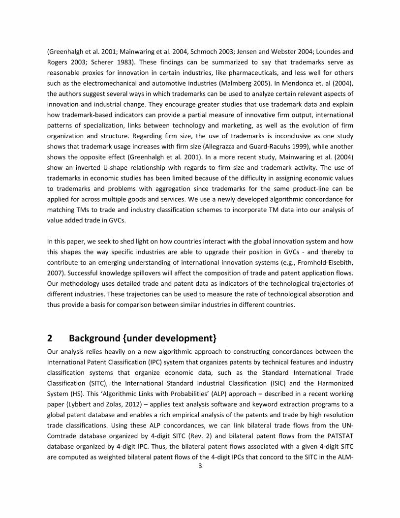
stage production process where intermediate goods are only used to produce final goods (as opposed to other intermediate goods). The benefit of this approach is that we only need to estimate the first-order influences of bilateral inputs2. This sequential feature of the production process is consistent with numerous production models such as Yi (2003, 2010), Baldwin and Venables (2010) and Costinot et al. (2011). Given this approximation of value-added trade, we can compute the value-added and gross exports using only the final goods and the intermediates directly used to produce the final goods. Hence, our measures of gross exports and value-added exports are constructed as:

�̅�𝑖𝑗 = 𝑓𝑖𝑗 + ∑ 𝐴𝑖𝑗𝑓𝑗𝑘𝑘

𝑣𝑎����𝑖𝑗 = 𝑓𝑖𝑗 + �𝐴𝑖𝑘𝑓𝑘𝑗𝑘

− �𝜄 ��𝐴𝑘𝑖𝑘

� 𝑑𝑖𝑎𝑔�𝑓𝑖𝑗��′

where [𝜄 [∑ 𝐴𝑘𝑖𝑘 ]𝑑𝑖𝑎𝑔�𝑓𝑖𝑗�]′ is a measure of the total intermediate input-use matrix for country i. To build intuition for the components of each figure, Johnson and Noguera further break down the figures starting with the gross exports �̅�𝑖𝑗. First, they decompose the pieces of the total sum of intermediate goods exported to a third party k. They note that the piece, 𝑓𝑖𝑗 + 𝐴𝑖𝑗𝑓𝑗𝑗 can be interpreted as a measure of the total “absorption” of goods from country i that are absorbed into country j as either a final good (𝑓𝑖𝑗) or intermediate good used to produce a final good consumed domestically (𝐴𝑖𝑗𝑓𝑗𝑗). Next, they note that the piece 𝐴𝑖𝑗𝑓𝑗𝑖 can be interpreted as “reflected” trade, since these are intermediate goods from country i to country j that end up eventually as final goods consumed in country i. This would be an example of outsourced production to country j taken by country i. The remainder, ∑ 𝐴𝑖𝑗𝑓𝑗𝑘𝑘≠𝑖,𝑗 , is then interpreted as “redirected” trade, since these are intermediate goods shipped from country i to country j that end as final goods consumed in country k. In addition, Johnson and Noguera break down the approximate value added exports 𝑣𝑎����𝑖𝑗. As we can see, once we break down the summation term, the value-added exports also include the “absorption” expression found in gross exports. However, for the value-added component, we need to subtract all of the imported intermediate inputs used prior to absorption. This create a “net absorption” term which consists of the absorption, 𝑓𝑖𝑗 + 𝐴𝑖𝑗𝑓𝑗𝑗 minus total intermediate use [𝜄 [∑ 𝐴𝑘𝑖𝑘 ]𝑑𝑖𝑎𝑔�𝑓𝑖𝑗�]′ plus the domestic intermediate use, 𝐴𝑖𝑖𝑓𝑖𝑗. Next, the expression ∑ 𝐴𝑖𝑘𝑓𝑘𝑗𝑘≠𝑖,𝑗 , can be characterized as “indirect exports” country j since the intermediates from country i comprise a share of the final good shipped from a third country k to country j. To summarize, using a two-stage sequential production process, 2 Johnson and Noguera say that higher order approximations may provide additional information to fit the data better, however, these higher orders add little to the overall measure of fragmentation.

(7)

(8)

7

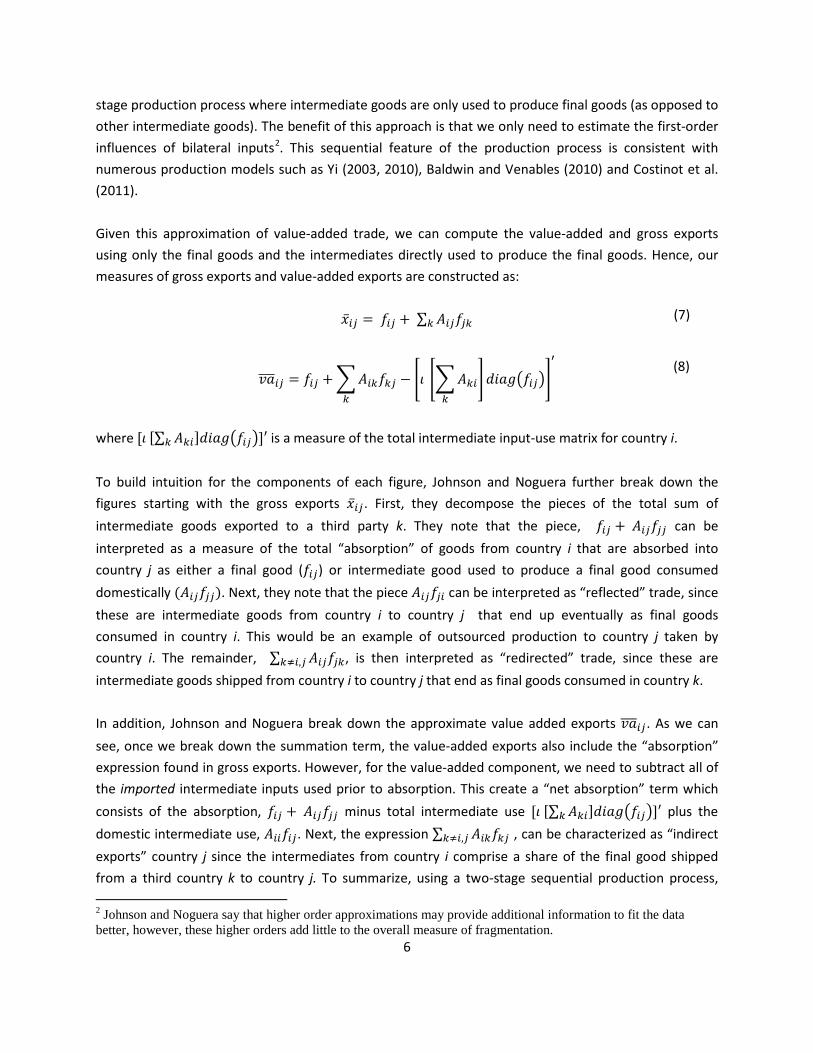
Johnson and Noguera construct values of gross exports and value-added exports using the I/O tables with the following components:

�̅�𝑖𝑗 = 𝑓𝑖𝑗 + 𝐴𝑖𝑗𝑓𝑗𝑗�������𝑎𝑏𝑠𝑜𝑟𝑝𝑡𝑖𝑜𝑛

+ 𝐴𝑖𝑗𝑓𝑗𝑖���𝑟𝑒𝑓𝑙𝑒𝑐𝑡𝑖𝑜𝑛

+ ∑ 𝐴𝑖𝑗𝑓𝑗𝑘𝑘�������𝑟𝑒𝑑𝑖𝑟𝑒𝑐𝑡𝑖𝑜𝑛

𝑣𝑎����𝑖𝑗 = 𝑓𝑖𝑗 + 𝐴𝑖𝑗𝑓𝑗𝑗 + 𝐴𝑖𝑖𝑓𝑖𝑗 − �𝜄 ��𝐴𝑘𝑖𝑘

� 𝑑𝑖𝑎𝑔�𝑓𝑖𝑗��′

�������������������������������𝑛𝑒𝑡 𝑎𝑏𝑠𝑜𝑟𝑝𝑡𝑖𝑜𝑛

+ � 𝐴𝑖𝑘𝑓𝑘𝑗𝑘≠𝑖,𝑗�������

𝑖𝑛𝑑𝑖𝑟𝑒𝑐𝑡 𝑒𝑥𝑝𝑜𝑟𝑡𝑠

We can then define the approximate VAX ratio as:

𝑉𝐴𝑋������𝑖𝑗 = 𝑣𝑎����𝑖𝑗�̅�𝑖𝑗

= 𝑛𝑒𝑡 𝑎𝑏𝑠𝑜𝑟𝑝𝑡𝑖𝑜𝑛𝑖𝑗 + 𝑖𝑛𝑑𝑖𝑟𝑒𝑐𝑡 𝑒𝑥𝑝𝑜𝑟𝑡𝑠𝑖𝑗

𝑎𝑏𝑠𝑜𝑟𝑝𝑡𝑖𝑜𝑛𝑖𝑗 + 𝑟𝑒𝑓𝑙𝑒𝑐𝑡𝑖𝑜𝑛𝑖𝑗 + 𝑟𝑒𝑑𝑖𝑟𝑒𝑐𝑡𝑖𝑜𝑛𝑖𝑗

Note that net absorption will always be less than absorption because it subtracts the value of all of the intermediate inputs used. Therefore, if there is no indirect trade, the approximate VAX ratio will always be less than one. Also note that if indirect exports are high enough, then the VAX ratio can exceed one. Since indirect exports are an outcome of production fragmentation (i.e. production processes happening elsewhere), this implies that a high approximate VAX ratio is indicative of increased production fragmentation. However, higher fragmentation also implies that “redirected” trade is also high, so that in the aggregate, these combined measures do not impact the VAX ratios too much. What does drive movements in the VAX ratio will be the following: (i) the difference between the “absorption” and “net absorption” measures and (ii) “reflected exports”. An increase in either “reflected” exports or in the difference between the absorption rates will drive the VAX ratio down – which is why the VAX ratio serves as a good proxy for production fragmentation since any movement in these two figures is driven by production happening away from the home country.

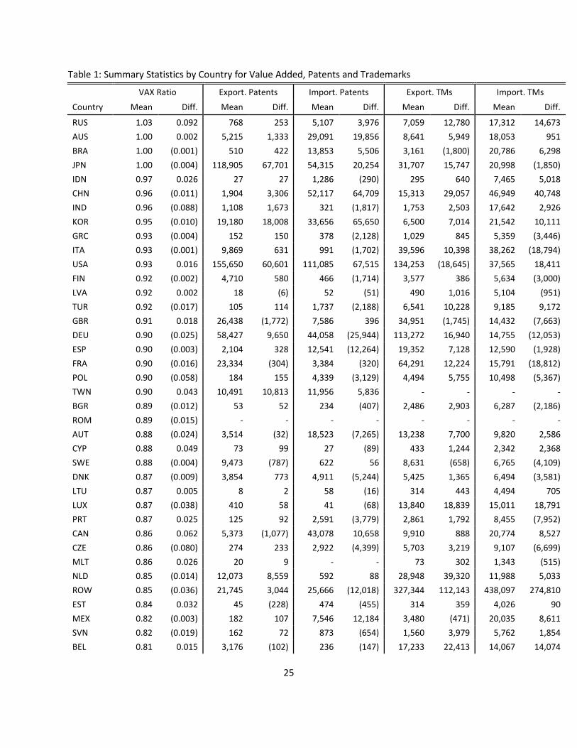
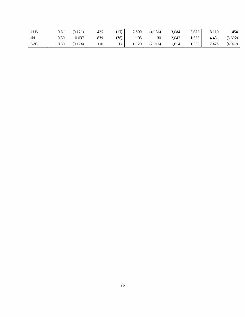
3.3 Construction using World Input-Output Database Now that the intuition and full methodology for calculating approximate VAX ratios has been established, we describe in detail the construction of bilateral VAX ratios using the WIOD database. For details of the WIOD database and its construction, we refer to Timmer (2012), which describes in details the contents, sources and methods used to construct the database. The database consists of 40 individual countries and 1 “Rest of World” country (“ROW”) and 35 industries encompassing agriculture, manufacturing, non-manufacturing and service activities from the year 1995 to 2009. For summary statistics on the countries and industries used, see Tables 1 and Tables 2. [TABLES 1 AND 2 HERE]

(9)

(10)

8

For each year, the WIOD database contains the standard I/O table (1435 × 1435 matrix) which consists of intermediate goods values 𝑚𝑖𝑗𝑡(𝑠, 𝑠′), as well as 5 columns each of which contain components of the final goods. These 5 columns were summed together for each country to provide our values for 𝑓𝑖𝑗, which is now a 1435 × 41 matrix. To compute our measures of 𝐴𝑖𝑗𝑡(𝑠, 𝑠′), we simply divide 𝑚𝑖𝑗𝑡(𝑠, 𝑠′) by the total output, which we defined in equation (1) as

𝑦𝑖𝑡(𝑠) = �𝑓𝑖𝑗𝑡(𝑠) + 𝑗

� �𝑚𝑖𝑗𝑡(𝑠, 𝑠′)𝑠′𝑗

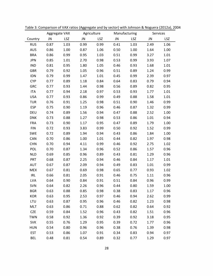
Once this figure is computed, it is relatively straightforward process to calculate each of the components of the gross exports and value-added exports (i.e. absorption, net absorption, etc…) using matrix algebra. Our end result once we perform the algebra are 1435 × 41 matrices for each of the components. These matrices are then transformed into bilateral country-industry pairs containing 58,835 observations for each year. These observations consist of the name of the home country, the industry being shipped and the destination country, along with each of the components of the VAX ratio. After tabulating for all of the years of the WIOD database, we are left with 882,525 bilateral country-industry observations. We can then collapse this dataset to analyze bilateral country-only observations, individual country-industry observations, individual country observations and individual industry observations. However, as we will see, we limit our analysis to country-industry bilateral pairs and aggregate country-industry measures due to the relative lack in variability in the aggregate measures across this limited time frame3. Since we are using the same methodology found in Johnson and Noguera, it makes sense to compare our initial ratios with theirs. However, it is important to mention that in both papers, Johnson and Noguera use different databases/values from the WIOD database and there is some discussion in their working paper about the limitations of the WIOD database. However, for the purposes of our study, which focus mainly on the bilateral country-industry relationship of value-added trade, we are more interested in this comparison to ensure that the trends and rankings are consistent rather than actual values. In Johnson and Noguera (2012a), they use the GTAP 7.1 Database which consists of the global I/O framework for 57 industries and 94 countries for 2004. We compare the cross-sectional country-level results of the WIOD for 2004 with these figures, which is found in Table 3. As we can see, there are some nontrivial discrepancies between the two measures where on average, the Johnson & Noguera (2012a) data has much higher VAX ratios for agriculture and services than our own measures. However, what is important to consider is the ranks between sectors and countries, both of which appear to be

3 See Johnson and Noguera (2012b) for a brief discussion in the footnotes discussing how the WIOD database fails to capture some important changes to the VAX ratios over time and how their study relies on the variability accrued over a four-decade long period.

9

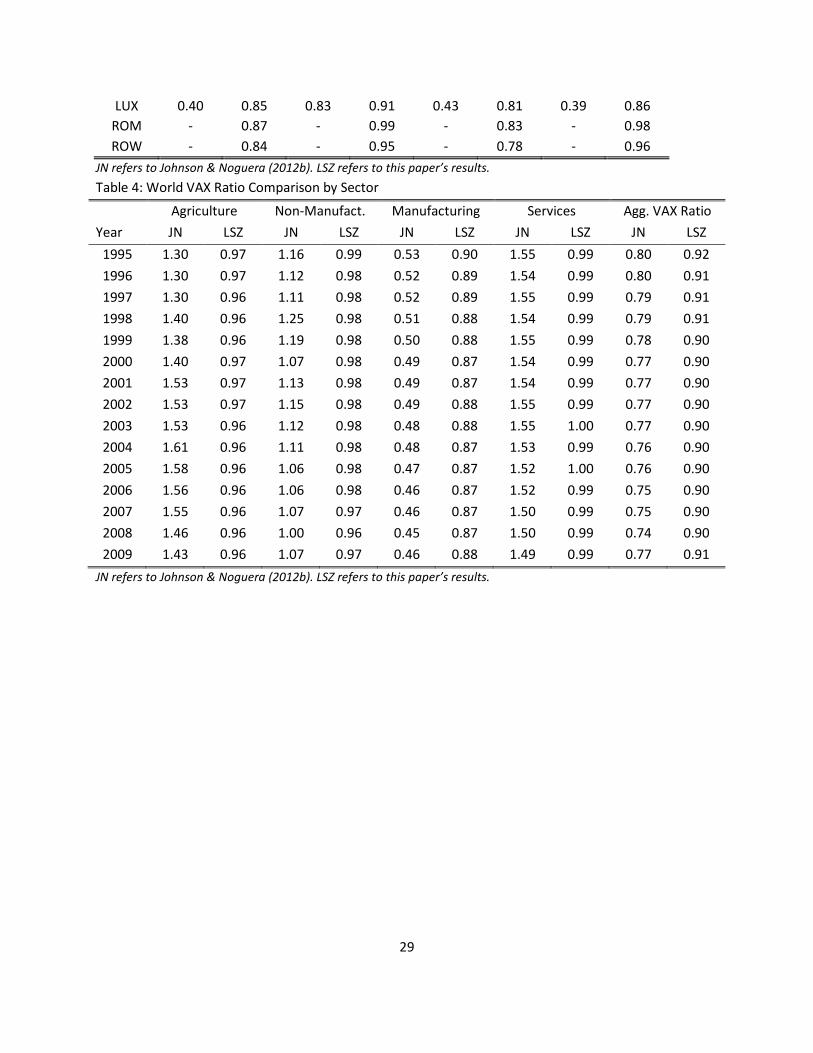
consistent in the sense that manufacturing typically has the lowest VAX ratios and countries that have the highest and lowest aggregate VAX ratios are very similar. [TABLE 3 HERE] Next, we compare our VAX ratio results with the latter Johnson and Noguera paper (2012b), which instead of containing a cross section, contains panel data over a 40-year period of VAX ratios for 42 countries. This data was constructed using trade data from the NBER-UN database and the CEPII BACI data, along with I/O tables from the OECD (1995 and 2011 versions) and IDE-JETRO. They then aggregate the industries into 4 sectors to make their calculations over the time period. It is also worth mentioning that for years where no I/O table was given, values were imputed. Given the difference in datasets and sectoral make-up, we expect to see some discrepencies between our results and theirs. Since they do not provide country-level results, we can only compare the World Value Added to Export ratio for the years 1995 to 2009. These results can be found in Table 4. [TABLE 4 HERE] We can see that the Johnson & Noguera (2012b) results have very different values for most of the sectors, with greater variability within each sector. This is most likely a result of the different methodologies and data used for the construction. However what is important is that the ranks of each sector and trends within each sector are more or less consistent. For instance, both agriculture and non-manufacturing all have higher VAX ratios than manufacturing and we see that the VAX ratios in both datasets decline over this time period and even tick upwards in 2009 together. Since the instructions to construct the VAX ratios are straightforward, we can be confident that no calculation errors occurred in the construction of our VAX ratios and that any differences are purely input related (in the case of the datasets used, time period, year of reference value). The primary concern we have with our data is the relative lack of heterogeneity found in the higher-levels of aggregation. Over the 15-year period, we can see that the worldwide aggregate VAX ratio moves downward only by two percentage points. Even when we disaggregate to the country-level measures, we see that the within sector variability typically is around 10-15 percentage points, which is quite low. Therefore, for these reasons, we limit our analysis to the country-industry level where we see plenty of movement between country-industries pairs. In the analysis that follows in the next section, we start our analysis by analyzing bilateral country-industry patterns of the VAX ratio. We then analyze how the aggregate country-industry VAX ratios are impacted by IP transfers, as well as how a country’s IP output is impacted by movement in their VAX ratios. First, however, we describe the other data we combine in this analysis.

3.4 Patent, Trademark & Other Data

10

In order to jointly analyze IP and value-added trade, we match bilateral patent and trademark data taken from the World Intellectual Property Organization (WIPO) with the WIOD database. To ensure property country-industry matches, we will first need to translate the classification system used for patents and trademarks into the industry classifications used in the WIOD database. The industries in the WIOD database are organized by ISIC class4. In order to concord the patent data, which is organized by the International Patent Classification (IPC) system, we utilized the concordance developed in Lybbert & Zolas (2012) which uses text analysis software to match technologies to industries. For the trademark data, which is organized by the NICE classification system, we used a similar “algorithmic links with probabilities” (ALP) concordance but specifically designed for trademarks (see Lybbert & Zolas (2013)) to convert the two digit NICE classes into the WIOD industries.5

Once the bilateral patent and trademark flows have been concorded to match the WIOD industry groups, we then incorporate proxies for trade costs, such as distance, border dummies, language dummies and colonial history taken from CEPII. This completes our data construction. Unfortunately, not all of the years of the patent and trademark data coincide with the WIOD data. For instance, the bilateral country-industry patent data exists from 1990 to 2003, which means that our analysis for patents can only take place in the eight years between 1995 and 2003. For trademarks, we have bilateral country-industry trademark flows only for 2004 to 2009.Both of these are limited time frames for any significant changes to the production process. Therefore, we expect the coefficients to be quite small. However, our interest lies more in the directional aspects of the coefficients, rather than specific values.

4 Value-Added Trade & IP Analysis Our primary interest in this paper is to analyze how patterns of production fragmentation are impacted when firms transfer their intellectual property (IP) in the form of patents and trademarks abroad. Depending on the type of patent (either a process or product patent), we expect varying results. For process patents (i.e. patents that relate to the improvement of a particular production process), it is easy to imagine that as firms export more process patents, then that would be indicative that the firm is planning on conducting more of their production outside of the country. This would imply that both “reflected” trade and “redirected” trade would increase in this scenario meaning that the VAX ratio would be expected to decline with increased patent transfer. On the other hand, for product patents, which are more likely to relate to the increased transfer of final goods, we would most likely see a different outcome to the VAX ratio. Higher levels of final goods exports would have a null affect on the “net absorption/absorption” ratios (the higher 𝑓𝑖𝑗𝑡(𝑠) would cancel out) and no affect on “redirected” or “reflected” trade. Instead, we would most likely see an increase of “indirect exports” following these 4 Although it is not clear which revision it is, it does not matter for our analysis, since we can match the industry groups of the WIOD database one-to-one for any ISIC revision. For methodology purposes, we matched the WIOD industries to the ISIC Rev. 4. 5 Both the Patent and TM concordances to WIOD industries are available by the authors.

11

patents, which would imply a higher VAX ratio. Unfortunately, we cannot differentiate between the two types of patents, however, we can look at the results and based on the changes to the VAX ratio, assess the types of patents that are being transferred. If we see reduced VAX ratios as a result of increased patent transfer, then we can assume that the country is transferring more process patents. On the other hand, if the VAX ratio increases as a result of increased patent exports, then it is likely that the country is exporting more product patents. For patents received by the home country (i.e. patent imports), we expect this to influence the final goods exports if the imported patents are process patents. For process patents, we also expect that “indirect exports” will increase, implying higher VAX ratios for imported process patents. As for imported product patents, this would only affect “reflected” trade, which leads towards lower VAX ratios. With exported trademarks, which are normally applied on final goods, we expect to see a similar affect as with exported product patents. Namely, since increased trademark transfer is more likely to be associated with increased final goods, we can expect to see “indirect exports” increase, along with the VAX ratio. For imported trademarks, our “reflected” trade should increase, leading to a lower VAX ratio. Therefore, to sum up our hypothesis regarding bilateral patent and trademark flows, if we find that patent exports lead to increased fragmentation then that is evidence that mainly process patents are being transferred. If the opposite is true, then that is an indication that product patents are the ones being exported. For imported patents, we expect to see higher VAX ratios for mainly imported process patents and lower VAX ratios for imported product patents. Turning our attention to exported trademarks, we expect to see lower fragmentation (i.e. higher VAX ratios) with increased TM exports and higher fragmentation with increased TM imports. In a similar vein, we are also curious as to how production fragmentation might impact domestic IP output. In a basic model of offshoring, increased production fragmentation allows the domestic firm to reallocate more workers towards higher-end production processes, of which R&D is typically considered one of them. Therefore, we would expect that countries who increase their production fragmentation over time to benefit with higher levels of innovation. Therefore, we expect to see that changes in the VAX ratio lead to higher outputs in patents and trademarks.

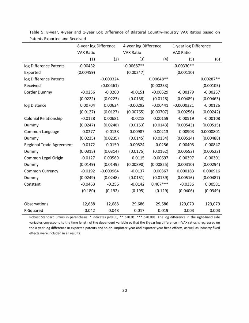
4.1 Bilateral Country-Industry Results Our first stage analysis looks at the change to VAX ratios over the aforementioned time period and regresses them based on trade costs and the change in patent and trademark export intensity and reception. We first look at patents over the years 1995-2003. Our regressions look at the change in the log of the VAX ratio over the entire 8-year period (1995-2003), over two 4-year periods (1995-1999, 200-2003) and each year, regressed on similar changes in the amount of exported patents per person and received patents per person. The results, displayed in Table 5, show that increased patent exports lead

12

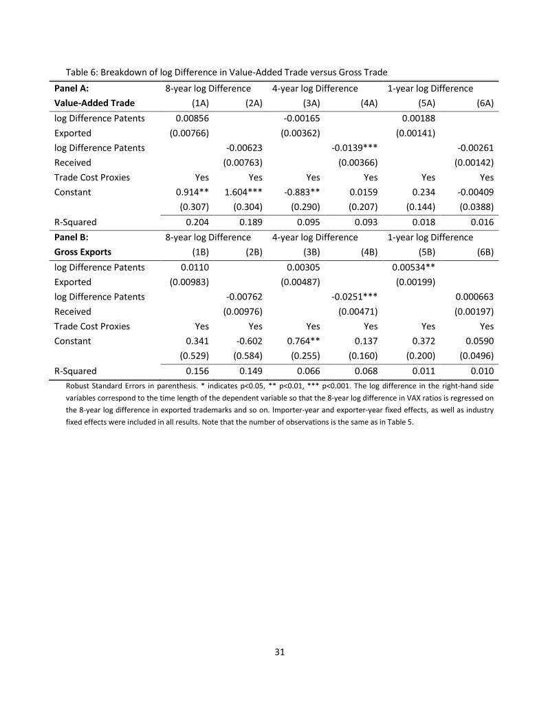
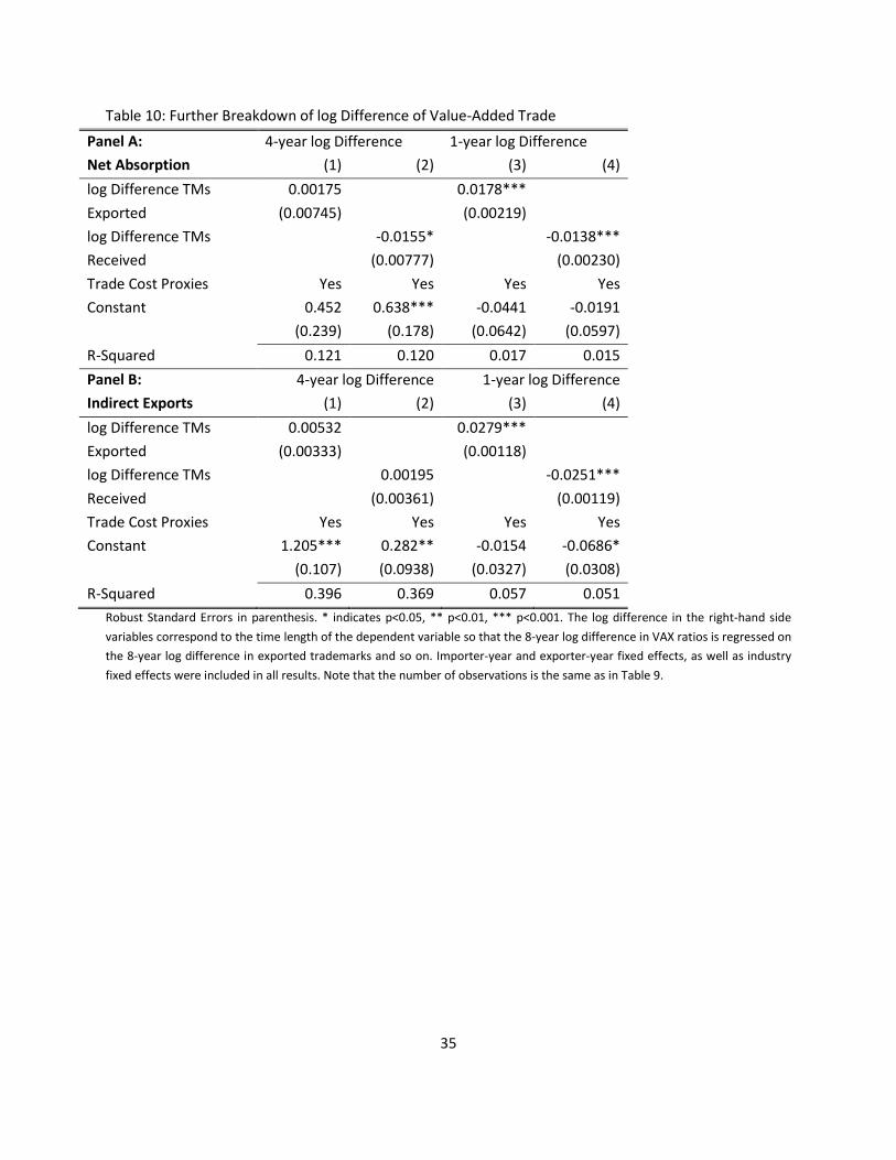
to increased fragmentation which suggests that mainly process patents are being transferred. Similarly, the fact that higher patent imports leads to higher VAX ratios is also suggestive that firms are transferring mainly process patents. These two results are early indications that firms mainly patent abroad to protect their production process. To further understand these results, we next assess where the movement in the VAX ratio is occurring. Our hypothesis predicts that we should see increased gross exports as a result of process patents being transferred. The results of separate regressions for value-added trade and gross exports are shown in Table 6. Interestingly, most of the movement seems to occur in the gross exports component of the VAX ratio which further supports our claim to process patents. We further deconstruct this relationship to now look at each of the components of gross exports. We expect to see most of the movement occurring in “reflected” and “redirected trade”. As expected and shown in Table 7, the outcome from increased patent transfer are higher levels of “reflected” and “redirected” trade, which are driving the movements in the VAX ratio. Therefore, it appears that most of the patents being transferred abroad are being used for production purposes and offshoring as opposed to protecting the invention of final goods. We next look at the effects of trademark transfers. Our hypothesis predicts that increased trademark exports will lead to increased VAX ratios (aka less production fragmenting) driven by higher levels of “indirect exports”. We also predict that increased trademark imports will lead to lower VAX ratios (aka increase production fragmentation) driven by higher levels of “reflected” trade. We can only analyze the period between 2004 and 2009. In keeping consistent with the 4-year time frame established with patents, our time horizon for the four-year log difference is 2004-2008. The results in Table 8 confirm our initial hypothesis that increased trademark transfer reduces production fragmentation. However, the effect of imported trademarks appears negligible. To figure out why this is the case, we can similarly deconstruct the impact of trademark exports by analyzing its impact on gross trade and value-added trade. Our earlier prediction said that we should see higher levels of value-added trade as a result of increased TM exports. As shown in Tables 9 and 10, most of the movement in the VAX ratio is driven by value-added trade. We can also see that there is movement in both gross exports and value-added exports from the imported TMs, which appear to cancel each other out. Next, we turn to the individual components of value-added trade to verify that the movement is happening through “indirect exports” as opposed to the absorption levels. It appears that most of the movement within the Value-Added exports is driven by the change in “indirect exports” which again, supports our hypothesis. We have run similar regressions for the gross exports and found comparable magnitudes and signs for the “absorption” variable and insignificant values for “reflected” and “redirected” trade. Our attention now turns to the aggregate Country-Industry VAX ratios and how they impact domestic innovation levels.

13

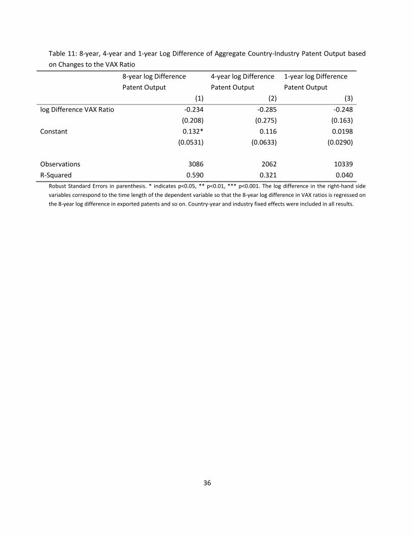
4.2 Individual Country-Industry Results We now turn our attention away from the bilateral flows to analyze how aggregate country-industry VAX ratios Influence innovation levels in the home country as measured by patent and trademarks. A simple offshoring model predicts that increased fragmentation, represented by lower VAX ratios, will lead to higher levels of innovation output in the home country driven by reallocating production to “higher value” activities such as R&D. We first turn to our patent results in Table 11. Although our results are insignificant, the pattern suggests that increased production fragmentation lead to higher levels of innovation growth. We next look at what happens to trademarks with increased fragmentation. Again, although the results (Table 12) are insignificant, we see that increased fragmentation has a positive effect on trademark output. Both of the patent and trademark results follow the simple offshoring model which hypothesizes that through increased offshoring, wealthy countries can focus their activities on higher-skilled processes, such as R&D. To summarize our findings, we have found that analyzing international IP flows can tell us quite a bit about the global production process. Increased international patent transfer positively contributes to higher levels of production fragmentation. This is suggestive that most of the patents being transferred abroad relate more to the production process, rather than final goods. Therefore, it appears that patents play an important role in the global value chains and international production process by protecting firms’ production abilities in foreign countries. On the other hand, the international transfer of trademarks, which relate more to products/final goods (rather than processes) tends to reduce production fragmentation since more value-added exports are emerging from the home country in the form of “indirect exports”. We also see that countries who receive more trademarks are more likely to offshore their production. The importance of these IP transfers also reveals how important the IP environment is for countries looking to attract multi-national investment. It appears that outside countries consider the IP environment in their investment decisions. Finally, the fragmentation of production has had a positive effect on the innovation rates occurring in the home country, which follows the basic model of offshoring.

5 Patents & GVCs: The Korean Electronics Experience One of the earlier examples of the spread of GVCs to Asia in post war years is the story of the Korean electronic industry, which was non-existent pre-1958 and by 1994 was the fourth largest global producer of electronics (after US, Japan and Germany) and the second largest producer of consumer electronics (after Japan)6. Similarly, in semiconductors, S. Korea that started as low cost assembler of discrete devices in the mid 1960s became 2nd largest producer of memory chips (that’s in 1997 - largest today?) and 3rd largest semiconductor producer (after Japan and US). This amazing revolution would not

6 Quote Linsun Kim book, pp.131

14

have been possible without the access to advanced technologies and markets assisted mainly by Foreign Licensing (FL) and OEM (a form of FDI) agreements. However, whereas Korea did strategically leverage its low cost to penetrate established markets, it did so while driving high its share of VA in the final product by trying to be in full control of producing as much of the components of the final product as possible. That system level approach, driven largely from above by the government, was key to the rapid assimilation of the new technologies and their diffusion throughout the Korean industry. Still, the beginnings of most of the major success stories in the Korean electronic industry were always in reverse engineering of existing successful products and establishing production while using imported key components (e.g. the magnetrons for the microwave ovens in the early 1980s and PC components in the mid to late 1980s), and only later, once the production line was well established and the local engineers fully owned the product design did they attempt to complete ownership through licensing or acquisition of the missing parts. The aggressive pursuit of technology licensing is reflected in the high royalty fees paid by Koreans ($1.75B in 1995.7 The insistence on being in full charge of their technological capabilities and product design also explains the second difference between today’s GVCs and the Korean case: whereas today it is the brand name firm that owns the product design that seeks opportunity to optimally outsource varying portions of the manufacturing, in the Korean case it was the Korean Chaebols that chose the markets and products that they want to produce and once they acquire the initial capability, sought the FLs and strategic alliances to facilitate their plans. Still, while the OEM agreements opened established markets to Korean access as well as challenged them with highly competitive quality standards and pricing demands, it also implied that their products were distributed under the foreign partner’s brand name rather than their own name and in that, the relationship resembles present day GVC relationships. 8. With these caveats in mind, the Korean electronic industry is still a poster child for a wildly successful trade driven technological convergence story that can help us gain in-depth understanding of the factors that make for such successful technological convergence. To that end we want to look at the evolution of that industry from a perspective of technology and trade flows, where the inflow of foreign patents into S. Korea indicates the technological fields affected by the FL and the outflows of trade and Korean patents registered abroad – the outcomes in the industries affected by that technology and the extent of assimilation of that technology in the receiving industry. The main portion of the story unfolded in the period between 1970-1995, when the industry’s output as a whole went from $30.4M to over $73B9. With close to 60% of production going to exports, trade data is a good indicator of the changes in the local economy. Ideally, with detailed break down of the trade flow as we have in the post 1988 data, we could have tracked more precisely the shifts in the industry as reflected by the specific traded commodities. Alas, up to 1987 trade data is aggregated at the 2-digits

7 WTEC Report on the Korean Electronics Industry, June 1997, http://www.wtec.org/loyola/kei/welcome.htm 8 The ratio EX/IM serves as a measure of the Korean Value Added – since we do not have the needed data to calculate more accurate VAX estimates. 9 Output estimate in 1995 encompasses all electronic and electrical equipment and assumes that 58% of the output of the industry as a whole was exported (based on Table 6-1 from K. Kim that quotes the Korea Development Bank, Korean Industry in the world, 1994)

15

SITC levels, providing a single annual figure for the whole electronic industry. Thus, the actual details for the specific make-up of the trade can be deduced from the IPR scene as divulged by the inflow of foreign patents into Korean and the later outflow from Korea to substantial trade partners. The methodology employed in this section comprises qualitative comparisons of patent and trade flows and their components, using the LZ concordance as a basis for correlating SITC/HS categories of trade and the IPC classification of patents. We bring forth two new elements: A comprehensive analysis (by WIPO technological field) of bilateral flow of electronic related patents between S. Korea and other countries starting between 1970-1995 and a concordance that maps main trade groupings as defined by the Asian IO tables to the WIPO IPC based technological fields. The data confirms much of the details that thus far has been available only as a prose narrative in various accounts of the evolution of the electronic industry and validates the use of these data to study the relationship between technology flow and economic outcomes as important tools in the study of economic growth and development.

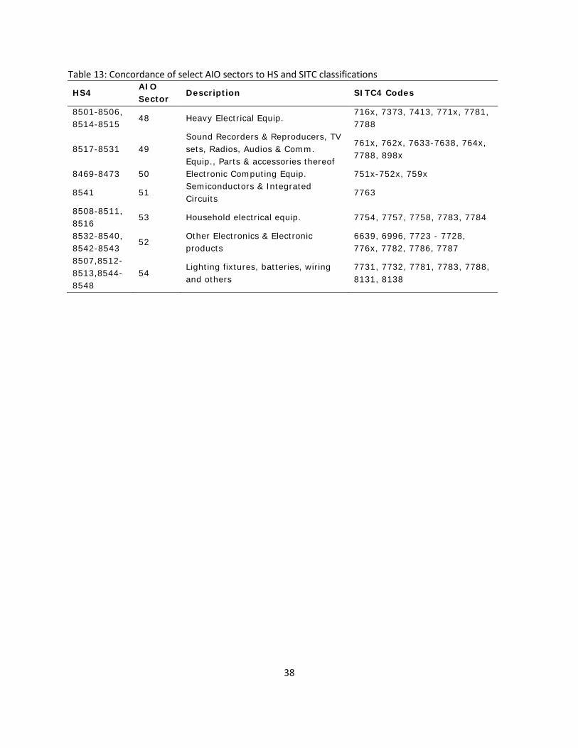
5.1 Data & Methodology The data used in the following analysis originates from a number of sources. The multilateral trade data between Korea and other countries for the period of 1970-1995 was taken from the UN Comtrade data base10. As mentioned above, a major change in the collection of the data has taken effect in 1988 resulting in higher levels of data disaggregation as well as shift in the classification from SITC Rev. 2 to HS 1992. As a result, there is some inconsistencies (discontinuity) in the data between the 1987 figures and the 1988 ones where there is a substantial jump in the total world exports and imports for the Electric and Electronic Equipment (classification 85) between these two years. The trade data was aggregated per the definition of the Asian International IO tables.11 The mapping between the SITC classification, HS and these groups for the electronic commodities is provided in Table 1. Notice that the only AIO sector outside the 85 HS2 code is 50 – Electronic Computing Equipment – which would have been reported under HS2 84 pre 1988. Judging from post 1987 data, where total HS2 84 export totals were $4.5B, out of which $2.5B were computing equipment exports. However, the computing equipment classification of the HS includes all forms of office equipment including typewriters, word processors and calculators as well as modern digital computers (e.g. PCs) and those were not exported in large numbers by Korea until the late 1980s. For the patent data – we were looking for patents whose application dates were between 1970-1995. Data for patents granted from 1978 on is available from the European Patent Office (EPO) and provides full bibliographical information for the patents in English. We used the PatStat 2008 version of the data base. For earlier data we went directly to the source – the Korean Patent Office web site and conducted a manual search for all patents with IPCs that belong to the Electrical Engineering WIPO sector and

10 http://comtrade.un.org/db/ 11 Quote Institute of Developing Economies, Japan, http://www.ide.go.jp/English/Research/Topics/Eco/Io/index.html

16

checked for the country of the applicant. Thus all patent information for 1970-1976 was obtained from the Korean IPR Information Service (KIPRIS)12. Since all patents applied for in 1977 were granted in 1978 or later – they were also obtained from the PATSTAT data base. Again, there is marked discontinuity technical field distribution of the data between the two sources of the data (KIPRIS and PATSTAT) – which may reflect the continuing adjustment of the IPCs for patents as the IPC structure evolves used by the EPO – whereas the Korean PTO classification may be static. Mapping between the patents, grouped under the WIPO technological fields, and the trade flows, grouped under the AIO sectors, was done using a concordance computed specifically for that purpose. The starting point for the concordance was the LZ SITC4 Rev. 2 to IPC concordance. We mapped the IPCs to the WIPO Technology Fields (WFLD) and computed the SITC to WFLD concordance. Then we mapped the AIO sectors to HS2012 and to SITC2 – resulting in mapping both from HS and AIO to WTF. Reverse mapping provides the WFLD to AIO sector mapping. We choose to ignore all sectors with less than 5% probability because of their small effect on the result.

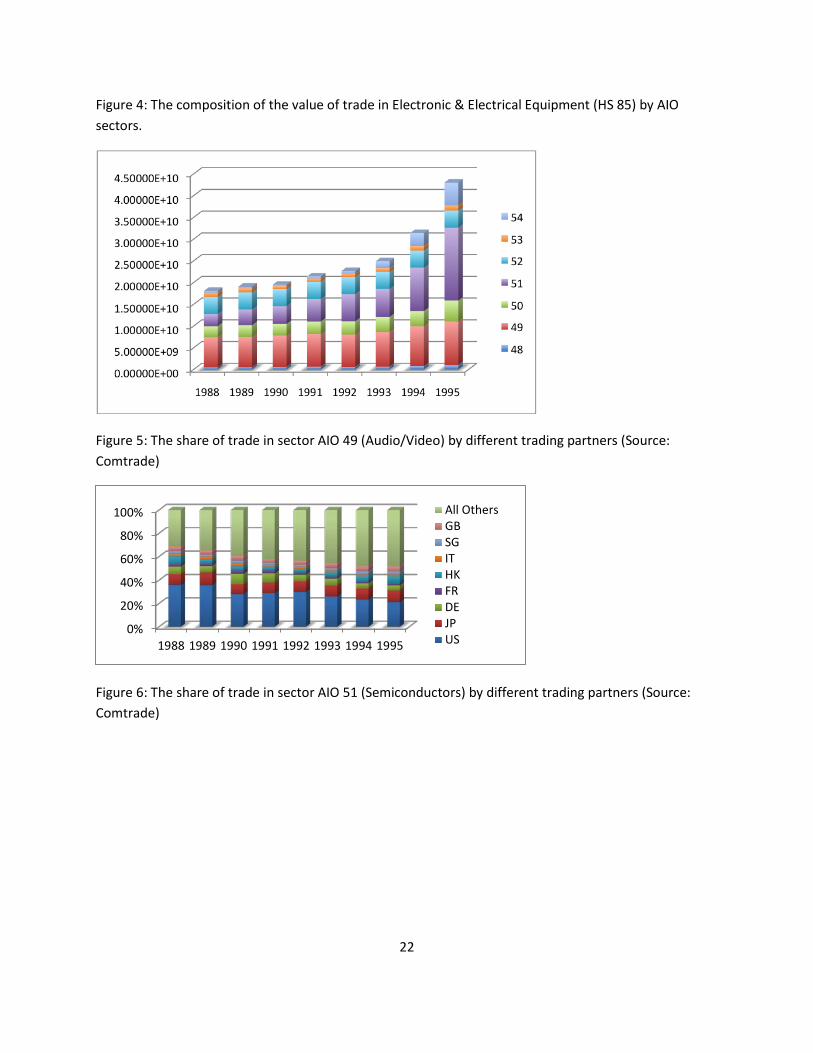
5.2 Analysis In the period of 1968-1973 there was a small number of foreign patents registered in Korea at all (663) with only 81 of them in the electrical engineering (EE) sector. in total for the period of ). In 1974 there is a big deluge of patents that pouring in (a total of 829) mainly from Japan (565) with 174 Japanese patents in the EE sector (particularly from Sony & Hitachi - color TV related)13. This one time event did not repeat itself and it is not until 1980 that we see the establishment of a consistent flow of foreign EE patents into Korea. The totals and their break-up into the specific technological fields are provided in Figure 1 & Figure 2. If the dominant fields in the earlier period are EE1 (Audio Visual Technology) and EE2 (Telecommunications) which reflect the entry of the industry into audio recording devices and telephones, then in the later period emphasis on the audio visual increase together with acquisition of electrical industrial machinery capabilities (EE0 – Electrical machinery, apparatus, energy) with the co-sprouting of the computer and semiconductor related technologies (EE5, EE7) starting in 1984. The key technological partners for the Korean electronic industry are overwhelmingly Japan with the US as a far second as evident from Figure 3. The composition of the corresponding trade data by AIO sectors for the period is provided in Figure 4. Clearly the dominant sectors are 49 (Audio & Video – the growth of the flat panel LCD screens market) and 51 (Semiconductors). Even before checking the concordance we know that these reflect very closely the general picture as portrayed by the patent data. Examination of the data for the Audio & Video equipment reveals a healthy diversity over a broad range of sub-categories – unlike the case of

12 http://engpat.kipris.or.kr/engpat/searchLogina.do?next=MainSearch 13 I did not find any specific reference to this event in the material that I reviewed nor a mention of any political inter-governmental agreement at the time, hence I have no explanation to what caused this Japanese rush (by a host of companies) to register their patents in Korea.

17

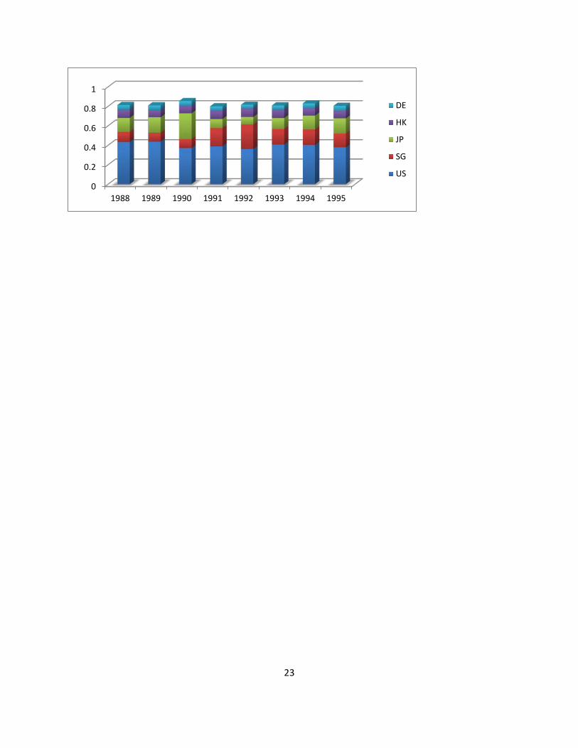
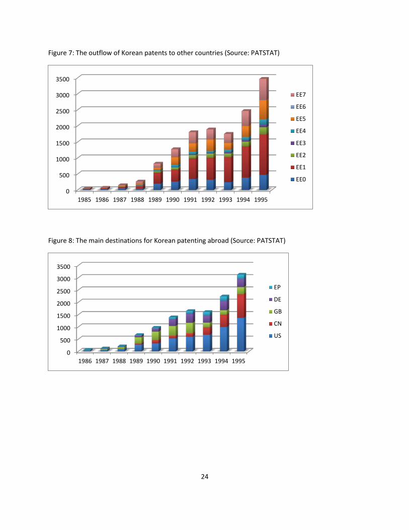
the semiconductors, which is completely monopolized by the DRAM. As for the main trading partners – here the special relationship with the US and Japan is well reflected14 (Figure 5 & Figure 6) – with both serving as willing markets for the electronic products of Korea – as implied by the OEM relationship that prevailed until the mid 1990s. In that sense – the relationship between Korea, the US and Japan is again reminiscent of the GVC – where the outsourcing firms are willing to provide the needed process technology to the producing firms. As Korea assimilated the technology and started upgrading in the supply chain to designing its own products and innovations, it made substantial investment in R&D, not the least through the establishment of global research centers. The successful results of this R&D investment represented a valuable IP that the Korean firms had interest in protection. As such – they started to register their own patents in countries around the world. Thus – is we look at the outflow of patents from Korea the picture (Figure 7) reflects the concentration of the industry, and its R&D, in the Digital Media (audio, video), computers and semiconductors. It is worth while noting that Korean firms has filed for many foreign patents prior to 1989, with only a small success15. The jump in the outflow of patents in 1989 may reflect a change in PTO patent processing rather than a function of the quality of the technology. Last but not least – the destinations for this outflow of patents – these are the major trading partners for Korea – with the exception of one – Japan (Figure 8). Its absence is very noticeable considering the close trade relationship that the two had over the years. If there was some agreement for reciprocal honoring of patents – we wouldn’t have seen the large number of patents arriving from Japan over the years. (Other possibilities??)

5.3 Discussion We would like to conclude with a few thoughts about the implication of the relationship that we have seen between the trade and patent data in the Korean electronic industry. First, the close relationship between the two confirms the practice among economists to infer technological flows from the content of trade flow. However, with the global patenting data becoming readily available we can use patent data together with the trade data as means of conducting diagnosis of the rate of technological absorption in a country. W can use patent inflow as triggering event to a local industry and monitor the output of the industry in way of tracking the progress.

14 Note in the Audio-Video market the shrinking shares of key partners resulting from the growing size and diversity of that group and thus declining dependency on the traditional key markets. This is however not the case for the semiconductors trade where the key partners and their total share changed very little over the period (with a marked shift from Japan to Singapore) 15 L. Kim (Table 6-2) quotes Samsung Electronic Company numbers regarding patent applications vs. granted statistics. In 1985 Samsung applied in Korea for 309 patents, and only 17 were granted, and internationally they applied at the same year for 32 patents out of which only 2 were granted. In 1990 – the firm applied in Korea for 1732 patents and was granted 640 and internationally, out of 1145 applications only 128 were granted.

18

On the larger scale of GVCs with production fragmented across multiple locales – the question is whether such fragments of production are sufficient to allow a country to assimilate the technology and upgrade in the value chain or is it boxed into its limited roll with no real options of growth. There are many lessons to be learned from the Korean experience but it seems that the central message is one of well coordinated effort at the local (national) level in order to maximize the benefits from the opportunities of market access of GVC.

6 Conclusion {under construction}

19

REFERENCES Awokuse, T.O., and H. Yin. 2010. "Intellectual property rights protection and the surge in FDI in china."

Journal of Comparative Economics 38(2):217-224. Baldwin, Richard and Anthony Venables. (2010). “Relocating the Value Chain: Offshoring and

Agglomeration in the Global Economy”. NBER Working Paper 16611. Bosworth, Derek, “Foreign Patent Flows To and From the United Kingdom,” Research Policy, Vol. 13,

No. 2, 1984. Coe, David and Elhanan Helpman, “International R&D Spillovers,” European Economic Review, Vol. 35,

No. 5, May 1995. Costinot, Arnaud, Jonathan Vogel and Su Wang (2011). “An Elementary Theory of Global Supply

Chains”. NBER Working Paper 16936. Eaton, Jonathan and Samuel Kortum, Josh Lerner, “International Patenting and the European Patent

Office: A Quantitative Assessment,” Patents, Innovation and Economic Performance: OECD Conference Proceedings, 2004.

Fromhold-Eisebith, M. 2007. "Bridging scales in innovation policies: How to link regional, national and international innovation systems." European Planning Studies 15(2):217-233.

Harhoff, Dietmar and Karin Hoisl, Bettina Reichl, Bruno Van Pottelsberghe De La Potterie, “Patent Validation at the Country Level: The Role of Fees and Translation Costs,” Research Policy, Vol. 38, No. 9, 2009.

Ivus, O. 2010. "Do stronger patent rights raise high-tech exports to the developing world?" Journal of International Economics 81(1):38-47.

Johnson, Robert C. and Guillrmo Noguera (2012a). “Accounting for Intermediates: Production Sharing and Trade in Value Added”. Journal of International Economics. 86(2)

Johnson, Robert C. and Guillermo Noguera. (2012b). “Fragmentation and Trade in Value Added Over Four Decades”. NBER Working Paper 18186.

Kim, Linsu 1997, “Imitation to Innovation - The Dynamics of Korea’s Technological Learning”, Harvard Business School Press.

Kim, Linsu, “Technology Transfer & Intellectual Property Rights – The Korean Experience”, Intellectual Property Rights and Sustainable Development, June 2003, UNCTAD-ICTSD project on IPRs and Sustainable Development.

Kim, Kiheung, “Technology Transfer: The Case of the Korean Electronics Industry”, The Hawaii Intenational Conference.

Lybbert, T.J. and N.J. Zolas. 2012 “Getting Patents & Economic Data to Speak to Each Other: An ‘Algorithmic Links with Probabilities’ Approach for Joint Analyses of Patenting & Economic Activity” WIPO Economics & Statistics Working Paper No.5, October.

Primo Braga, C., and C. Fink. 1999. "How stronger protection of intellectual property rights affects international trade flows." World Bank Policy Research Working Paper (2051).

Slama, Jiri, “Analysis by Means of a Gravitation Model of International Flows of Patent Applications in the Period 1967 – 1978,” World patent Information, Vol. 3, No. 1, 1981.

20

Timmer, Marcel. (2012). “The World Input-Output Database (WIOD): Contents, Sources and Methods.” WIOD Working Paper Number 10.

Vichyanond, J. 2009. Intellectual property protection and patterns of trade: Center for Economic Policy Studies, Princeton University.

Yi, Kei-Mu (2003). “Can Vertical Specialization Explain the Growth of World Trade?” Journal of Political Economy, 111.

Yi, Kei-Mu (2010). “Can Multi-Stage Production Explain the Home Bias in Trade?” American Economic Review, 100(1).

21

Figure 1: Inflow of EE patents into Korea, 1970-76 (Source: KIPRIS)

Figure 2: Inflow of EE patents into Korea, 1977-95 (Source: PATSTAT)

Figure 3: The main sources of foreign patents flowing into Korea, 1974,92 (Source: PATSTAT)

0

50

100

150

200

250

1970 1971 1972 1973 1974 1975 1976

EE7

EE6

EE5

EE4

EE3

EE2

EE1

0

500

1000

1500

2000

1974 1976 1978 1980 1982 1984 1986 1988 1990 1992

All Others

FR

NL

DE

US

JP

22

Figure 4: The composition of the value of trade in Electronic & Electrical Equipment (HS 85) by AIO sectors.

Figure 5: The share of trade in sector AIO 49 (Audio/Video) by different trading partners (Source: Comtrade)

Figure 6: The share of trade in sector AIO 51 (Semiconductors) by different trading partners (Source: Comtrade)

0%

20%

40%

60%

80%

100%

1988 1989 1990 1991 1992 1993 1994 1995

All OthersGBSGITHKFRDEJPUS

23

0

0.2

0.4

0.6

0.8

1

1988 1989 1990 1991 1992 1993 1994 1995

DE

HK

JP

SG

US

24

Figure 7: The outflow of Korean patents to other countries (Source: PATSTAT)

Figure 8: The main destinations for Korean patenting abroad (Source: PATSTAT)

0

500

1000

1500

2000

2500

3000

3500

1985 1986 1987 1988 1989 1990 1991 1992 1993 1994 1995

EE7

EE6

EE5

EE4

EE3

EE2

EE1

EE0

0

500

1000

1500

2000

2500

3000

3500

1986 1987 1988 1989 1990 1991 1992 1993 1994 1995

EP

DE

GB

CN

US

25

Table 1: Summary Statistics by Country for Value Added, Patents and Trademarks

VAX Ratio Export. Patents Import. Patents Export. TMs Import. TMs Country Mean Diff. Mean Diff. Mean Diff. Mean Diff. Mean Diff.

RUS 1.03 0.092 768 253 5,107 3,976 7,059 12,780 17,312 14,673 AUS 1.00 0.002 5,215 1,333 29,091 19,856 8,641 5,949 18,053 951 BRA 1.00 (0.001) 510 422 13,853 5,506 3,161 (1,800) 20,786 6,298 JPN 1.00 (0.004) 118,905 67,701 54,315 20,254 31,707 15,747 20,998 (1,850) IDN 0.97 0.026 27 27 1,286 (290) 295 640 7,465 5,018 CHN 0.96 (0.011) 1,904 3,306 52,117 64,709 15,313 29,057 46,949 40,748 IND 0.96 (0.088) 1,108 1,673 321 (1,817) 1,753 2,503 17,642 2,926 KOR 0.95 (0.010) 19,180 18,008 33,656 65,650 6,500 7,014 21,542 10,111 GRC 0.93 (0.004) 152 150 378 (2,128) 1,029 845 5,359 (3,446) ITA 0.93 (0.001) 9,869 631 991 (1,702) 39,596 10,398 38,262 (18,794) USA 0.93 0.016 155,650 60,601 111,085 67,515 134,253 (18,645) 37,565 18,411 FIN 0.92 (0.002) 4,710 580 466 (1,714) 3,577 386 5,634 (3,000) LVA 0.92 0.002 18 (6) 52 (51) 490 1,016 5,104 (951) TUR 0.92 (0.017) 105 114 1,737 (2,188) 6,541 10,228 9,185 9,172 GBR 0.91 0.018 26,438 (1,772) 7,586 396 34,951 (1,745) 14,432 (7,663) DEU 0.90 (0.025) 58,427 9,650 44,058 (25,944) 113,272 16,940 14,755 (12,053) ESP 0.90 (0.003) 2,104 328 12,541 (12,264) 19,352 7,128 12,590 (1,928) FRA 0.90 (0.016) 23,334 (304) 3,384 (320) 64,291 12,224 15,791 (18,812) POL 0.90 (0.058) 184 155 4,339 (3,129) 4,494 5,755 10,498 (5,367) TWN 0.90 0.043 10,491 10,813 11,956 5,836 - - - - BGR 0.89 (0.012) 53 52 234 (407) 2,486 2,903 6,287 (2,186) ROM 0.89 (0.015) - - - - - - - - AUT 0.88 (0.024) 3,514 (32) 18,523 (7,265) 13,238 7,700 9,820 2,586 CYP 0.88 0.049 73 99 27 (89) 433 1,244 2,342 2,368 SWE 0.88 (0.004) 9,473 (787) 622 56 8,631 (658) 6,765 (4,109) DNK 0.87 (0.009) 3,854 773 4,911 (5,244) 5,425 1,365 6,494 (3,581) LTU 0.87 0.005 8 2 58 (16) 314 443 4,494 705 LUX 0.87 (0.038) 410 58 41 (68) 13,840 18,839 15,011 18,791 PRT 0.87 0.025 125 92 2,591 (3,779) 2,861 1,792 8,455 (7,952) CAN 0.86 0.062 5,373 (1,077) 43,078 10,658 9,910 888 20,774 8,527 CZE 0.86 (0.080) 274 233 2,922 (4,399) 5,703 3,219 9,107 (6,699) MLT 0.86 0.026 20 9 - - 73 302 1,343 (515) NLD 0.85 (0.014) 12,073 8,559 592 88 28,948 39,320 11,988 5,033 ROW 0.85 (0.036) 21,745 3,044 25,666 (12,018) 327,344 112,143 438,097 274,810 EST 0.84 0.032 45 (228) 474 (455) 314 359 4,026 90 MEX 0.82 (0.003) 182 107 7,546 12,184 3,480 (471) 20,035 8,611 SVN 0.82 (0.019) 162 72 873 (654) 1,560 3,979 5,762 1,854 BEL 0.81 0.015 3,176 (102) 236 (147) 17,233 22,413 14,067 14,074

26

HUN 0.81 (0.121) 425 (17) 2,899 (4,156) 3,084 3,626 8,110 458 IRL 0.80 0.037 839 (76) 108 30 2,042 1,556 4,431 (3,692) SVK 0.80 (0.124) 110 14 1,320 (2,016) 1,614 1,308 7,478 (4,927)

27

Table 2: Summary Statistics by Industry for Value Added, Patents and Trademarks

VAX Ratio Export. Patents Export. TMs Industry Description Mean Diff. Mean Diff. Mean Diff. Wholesale Trade 1.04 0.034 - - 55,748 (1,696) Inland Transport 1.02 0.013 394 96 4,001 550 Private Households 1.00 (0.035) - - - - Mining and Quarrying 0.99 (0.020) 17,278 1,803 18,411 1,769 Wood and Products of Wood and Cork 0.99 0.006 3,037 613 17,909 (694)

Retail Trade 0.99 0.003 - - 72,675 (2,721) Other Transport Activities 0.99 (0.011) 467 50 11,168 2,333 Financial Intermediation 0.99 (0.015) 16,793 9,128 26,302 6,154 Real Estate Activities 0.99 (0.016) - - 1,858 449 Education 0.99 (0.001) - - 10,442 2,512 Other Non-Metallic Mineral 0.98 0.003 13,333 2,681 22,527 (1,279) Sale and Repair of Motor Vehicles 0.98 0.009 1,437 371 11,659 1,817 Water Transport 0.98 (0.017) - - 3,083 447 Post and Telecommunications 0.98 (0.009) 13,354 8,972 30,218 4,295 Renting and Other Business Activities 0.98 0.010 70,524 39,294 91,296 18,375 Hotels and Restaurants 0.97 (0.002) 5,064 1,638 14,385 4,116 Public Admin and Defense 0.97 (0.022) 67 (9) 10,249 5,620 Other Social and Personal Services 0.97 (0.010) 5,194 1,518 56,767 10,147 Agriculture, Forestry and Fishing 0.96 (0.004) 20,780 3,370 51,372 (4,763) Basic Metals and Fabricated Metal 0.96 0.013 35,358 10,566 42,124 656 Health and Social Work 0.96 (0.011) 9,082 2,607 21,777 5,579 Pulp, Paper, Printing and Publishing 0.94 (0.006) 13,020 4,282 38,690 (2,151) Rubber and Plastics 0.94 0.006 4,115 924 15,439 (484) Electricity, Gas and Water Supply 0.94 (0.003) 9,849 1,191 23,753 2,139 Construction 0.94 0.020 13,115 4,250 24,921 2,918 Air Transport 0.94 (0.018) - - 1,140 166 Food, Beverages and Tobacco 0.91 (0.013) 21,944 6,641 86,633 (11,679) Chemicals and Chemical Products 0.91 (0.052) 74,309 11,234 80,518 (6,645) Leather, Leather and Footwear 0.88 0.013 6,723 1,981 20,018 (788) Machinery, Nec 0.88 (0.026) 25,439 10,908 57,720 (929) Textiles and Textile Products 0.87 0.016 14,382 5,220 76,869 (3,711) Manufacturing, Nec; Recycling 0.87 (0.034) 18,907 5,285 60,466 2,828 Electrical and Optical Equipment 0.85 (0.016) 68,008 46,408 63,156 1,796 Coke and Refined Petroleum 0.83 (0.053) 6,873 111 6,087 562 Transport Equipment 0.83 0.009 12,190 3,323 29,235 3,050

28

Table 3: Comparison of VAX ratios (Aggregate and by sector) with Johnson & Noguera (2012a), 2004 Aggregate VAX Agriculture Manufacturing Services Country JN LSZ JN LSZ JN LSZ JN LSZ

RUS 0.87 1.03 0.99 0.99 0.41 1.03 2.49 1.06 AUS 0.86 1.00 0.87 1.06 0.50 1.00 1.64 1.00 BRA 0.86 0.99 0.95 1.03 0.51 0.99 3.27 1.01 JPN 0.85 1.01 2.70 0.98 0.53 0.99 3.93 1.07 IND 0.81 0.95 1.80 1.05 0.46 0.93 1.68 1.01 GBR 0.79 0.92 1.05 0.96 0.51 0.89 1.24 0.99 IDN 0.79 0.99 1.47 1.01 0.45 0.99 2.39 0.97 CYP 0.77 0.89 1.18 0.84 0.64 0.83 0.79 0.94 GRC 0.77 0.93 1.44 0.98 0.56 0.89 0.82 0.95 ITA 0.77 0.94 2.18 0.97 0.53 0.93 1.77 1.01 USA 0.77 0.93 0.86 0.99 0.49 0.88 1.58 1.01 TUR 0.76 0.91 1.25 0.98 0.51 0.90 1.46 0.99 ESP 0.75 0.90 1.19 0.96 0.46 0.87 1.32 0.99 DEU 0.74 0.89 1.56 0.94 0.47 0.88 2.52 1.00 DNK 0.73 0.88 1.27 0.98 0.53 0.86 1.01 0.94 FRA 0.73 0.90 1.17 0.95 0.47 0.89 1.79 1.00 FIN 0.72 0.93 3.83 0.99 0.50 0.92 1.52 0.99

SWE 0.72 0.89 1.94 0.94 0.43 0.86 1.84 1.00 CAN 0.70 0.86 1.00 1.01 0.44 0.82 1.97 0.98 CHN 0.70 0.94 4.11 0.99 0.46 0.92 2.75 1.02 POL 0.70 0.87 1.34 0.96 0.52 0.86 1.57 0.96 NLD 0.69 0.85 0.96 0.89 0.43 0.81 1.29 0.96 PRT 0.68 0.87 2.25 0.94 0.46 0.84 1.17 1.01 AUT 0.67 0.87 2.09 0.94 0.49 0.83 1.01 0.99 MEX 0.67 0.81 0.69 0.98 0.65 0.77 0.93 1.02 IRL 0.66 0.81 2.05 0.91 0.46 0.75 1.11 0.96 LVA 0.64 0.90 0.84 0.91 0.51 0.84 0.96 0.99 SVN 0.64 0.82 2.26 0.96 0.44 0.80 1.59 1.00 BGR 0.63 0.88 0.85 0.98 0.38 0.83 1.17 0.96 KOR 0.63 0.95 2.53 0.97 0.46 0.94 2.62 0.99 LTU 0.63 0.87 0.95 0.96 0.46 0.82 1.23 0.98 MLT 0.63 0.86 0.71 0.88 0.62 0.82 0.64 0.92 CZE 0.59 0.84 1.52 0.96 0.43 0.82 1.51 0.96

TWN 0.58 0.92 1.36 0.92 0.39 0.92 3.18 0.95 SVK 0.55 0.76 1.29 0.95 0.39 0.72 1.77 0.96 HUN 0.54 0.80 0.96 0.96 0.38 0.76 1.39 0.98 EST 0.53 0.86 1.07 0.91 0.34 0.83 0.94 0.97 BEL 0.48 0.81 0.54 0.89 0.32 0.77 1.29 0.97

29

LUX 0.40 0.85 0.83 0.91 0.43 0.81 0.39 0.86 ROM - 0.87 - 0.99 - 0.83 - 0.98 ROW - 0.84 - 0.95 - 0.78 - 0.96

JN refers to Johnson & Noguera (2012b). LSZ refers to this paper’s results. Table 4: World VAX Ratio Comparison by Sector

Agriculture Non-Manufact. Manufacturing Services Agg. VAX Ratio Year JN LSZ JN LSZ JN LSZ JN LSZ JN LSZ

1995 1.30 0.97 1.16 0.99 0.53 0.90 1.55 0.99 0.80 0.92 1996 1.30 0.97 1.12 0.98 0.52 0.89 1.54 0.99 0.80 0.91 1997 1.30 0.96 1.11 0.98 0.52 0.89 1.55 0.99 0.79 0.91 1998 1.40 0.96 1.25 0.98 0.51 0.88 1.54 0.99 0.79 0.91 1999 1.38 0.96 1.19 0.98 0.50 0.88 1.55 0.99 0.78 0.90 2000 1.40 0.97 1.07 0.98 0.49 0.87 1.54 0.99 0.77 0.90 2001 1.53 0.97 1.13 0.98 0.49 0.87 1.54 0.99 0.77 0.90 2002 1.53 0.97 1.15 0.98 0.49 0.88 1.55 0.99 0.77 0.90 2003 1.53 0.96 1.12 0.98 0.48 0.88 1.55 1.00 0.77 0.90 2004 1.61 0.96 1.11 0.98 0.48 0.87 1.53 0.99 0.76 0.90 2005 1.58 0.96 1.06 0.98 0.47 0.87 1.52 1.00 0.76 0.90 2006 1.56 0.96 1.06 0.98 0.46 0.87 1.52 0.99 0.75 0.90 2007 1.55 0.96 1.07 0.97 0.46 0.87 1.50 0.99 0.75 0.90 2008 1.46 0.96 1.00 0.96 0.45 0.87 1.50 0.99 0.74 0.90 2009 1.43 0.96 1.07 0.97 0.46 0.88 1.49 0.99 0.77 0.91

JN refers to Johnson & Noguera (2012b). LSZ refers to this paper’s results.

30

Table 5: 8-year, 4-year and 1-year Log Difference of Bilateral Country-Industry VAX Ratios based on Patents Exported and Received

8-year log Difference 4-year log Difference 1-year log Difference VAX Ratio VAX Ratio VAX Ratio (1) (2) (3) (4) (5) (6) log Difference Patents -0.00432 -0.00687** -0.00330** Exported (0.00459) (0.00247) (0.00110) log Difference Patents -0.000324 0.00648** 0.00287** Received (0.00461) (0.00233) (0.00105) Border Dummy -0.0256 -0.0200 -0.0151 -0.00529 -0.00179 -0.00257 (0.0222) (0.0223) (0.0138) (0.0128) (0.00489) (0.00463) log Distance 0.00704 0.00624 -0.00292 -0.00441 -0.0000321 -0.00126 (0.0127) (0.0127) (0.00765) (0.00707) (0.00256) (0.00242) Colonial Relationship -0.0128 0.00681 -0.0218 0.00159 -0.00519 -0.00108 Dummy (0.0247) (0.0248) (0.0153) (0.0143) (0.00543) (0.00515) Common Language 0.0277 -0.0138 0.00987 0.00213 0.00903 0.0000801 Dummy (0.0235) (0.0235) (0.0145) (0.0134) (0.00514) (0.00488) Regional Trade Agreement 0.0172 0.0150 -0.00524 -0.0256 -0.00405 -0.00847 Dummy (0.0315) (0.0314) (0.0175) (0.0162) (0.00552) (0.00522) Common Legal Origin -0.0127 0.00569 0.0115 -0.00697 -0.00397 -0.00301 Dummy (0.0149) (0.0149) (0.00890) (0.00825) (0.00310) (0.00294) Common Currency -0.0192 -0.000964 -0.0137 0.00367 0.000183 0.000916 Dummy (0.0249) (0.0248) (0.0151) (0.0139) (0.00516) (0.00487) Constant -0.0463 -0.256 -0.0142 0.467*** -0.0336 0.00581 (0.180) (0.192) (0.195) (0.129) (0.0406) (0.0349) Observations 12,688 12,688 29,686 29,686 129,079 129,079 R-Squared 0.042 0.048 0.017 0.019 0.003 0.003

Robust Standard Errors in parenthesis. * indicates p<0.05, ** p<0.01, *** p<0.001. The log difference in the right-hand side variables correspond to the time length of the dependent variable so that the 8-year log difference in VAX ratios is regressed on the 8-year log difference in exported patents and so on. Importer-year and exporter-year fixed effects, as well as industry fixed effects were included in all results.

31

Table 6: Breakdown of log Difference in Value-Added Trade versus Gross Trade

Panel A: Value-Added Trade

8-year log Difference 4-year log Difference 1-year log Difference (1A) (2A) (3A) (4A) (5A) (6A)

log Difference Patents 0.00856 -0.00165 0.00188 Exported (0.00766) (0.00362) (0.00141) log Difference Patents -0.00623 -0.0139*** -0.00261 Received (0.00763) (0.00366) (0.00142) Trade Cost Proxies Yes Yes Yes Yes Yes Yes Constant 0.914** 1.604*** -0.883** 0.0159 0.234 -0.00409 (0.307) (0.304) (0.290) (0.207) (0.144) (0.0388) R-Squared 0.204 0.189 0.095 0.093 0.018 0.016 Panel B: Gross Exports

8-year log Difference 4-year log Difference 1-year log Difference (1B) (2B) (3B) (4B) (5B) (6B)

log Difference Patents 0.0110 0.00305 0.00534** Exported (0.00983) (0.00487) (0.00199) log Difference Patents -0.00762 -0.0251*** 0.000663 Received (0.00976) (0.00471) (0.00197) Trade Cost Proxies Yes Yes Yes Yes Yes Yes Constant 0.341 -0.602 0.764** 0.137 0.372 0.0590 (0.529) (0.584) (0.255) (0.160) (0.200) (0.0496) R-Squared 0.156 0.149 0.066 0.068 0.011 0.010

Robust Standard Errors in parenthesis. * indicates p<0.05, ** p<0.01, *** p<0.001. The log difference in the right-hand side variables correspond to the time length of the dependent variable so that the 8-year log difference in VAX ratios is regressed on the 8-year log difference in exported trademarks and so on. Importer-year and exporter-year fixed effects, as well as industry fixed effects were included in all results. Note that the number of observations is the same as in Table 5.

32

Table 7: Further Breakdown of log Difference of Gross Exports

Panel A: Absorption 8-year log Difference 4-year log Difference 1-year log Difference (1A) (2A) (3A) (4A) (5A) (6A) log Difference Patents 0.0121 0.00192 0.00489* Exported (0.00985) (0.00489) (0.00200) log Difference Patents -0.00766 -0.0261*** 0.000359 Received (0.00978) (0.00473) (0.00198) Trade Cost Proxies Yes Yes Yes Yes Yes Yes Constant 0.348 -0.571 0.772** -0.0745 0.377 0.0531 (0.530) (0.584) (0.256) (0.259) (0.201) (0.0499) R-Squared 0.154 0.147 0.064 0.066 0.011 0.010 Panel B: Reflected 8-year log Difference 4-year log Difference 1-year log Difference (1B) (2B) (3B) (4B) (5B) (6B) log Difference Patents -0.000743 0.0156** 0.00836*** Exported (0.0115) (0.00577) (0.00243) log Difference Patents -0.0211 0.0194*** 0.00780*** Received (0.0114) (0.00570) (0.00236) Trade Cost Proxies Yes Yes Yes Yes Yes Yes Constant 0.695 -0.425 0.398 0.493* 0.202* 0.466*** (0.658) (0.667) (0.316) (0.193) (0.0894) (0.0747) R-Squared 0.216 0.249 0.104 0.115 0.016 0.018 Panel C: Redirected 8-year log Difference 4-year log Difference 1-year log Difference (1C) (2C) (3C) (4C) (5C) (6C) log Difference Patents 0.0209* 0.0154** 0.00666** Exported (0.0105) (0.00520) (0.00214) log Difference Patents -0.00349 -0.00945 0.000597 Received (0.0105) (0.00515) (0.00214) Trade Cost Proxies Yes Yes Yes Yes Yes Yes Constant 0.914** 1.604*** -0.883** 0.0159 0.234 -0.00409 (0.307) (0.304) (0.290) (0.207) (0.144) (0.0388) R-Squared 0.204 0.189 0.095 0.093 0.018 0.016

Robust Standard Errors in parenthesis. * indicates p<0.05, ** p<0.01, *** p<0.001. The log difference in the right-hand side variables correspond to the time length of the dependent variable so that the 8-year log difference in VAX ratios is regressed on the 8-year log difference in exported trademarks and so on. Importer-year and exporter-year fixed effects, as well as industry fixed effects were included in all results. Note that the number of observations is the same as in Table 5.

33

Table 8: 4-year and 1-year Log Difference of Bilateral Country-Industry VAX Ratios based on Trademarks Exported and Received

4-year log Difference 1-year log Difference VAX Ratio VAX Ratio (1) (2) (3) (4) log Difference TMs 0.00662 0.00374** Exported (0.00385) (0.00115) log Difference TMs 0.00179 0.00111 Received (0.00403) (0.00125) Border Dummy 0.00161 -0.00105 0.00240 0.000845 (0.0160) (0.0168) (0.00473) (0.00512) log Distance -0.000287 0.0146 -0.00147 -0.00157 (0.00924) (0.00966) (0.00273) (0.00295) Colonial Relationship -0.0482** -0.0193 -0.00946 -0.00497 Dummy (0.0187) (0.0196) (0.00556) (0.00601) Common Language 0.0305 0.0492* 0.00680 0.00988 Dummy (0.0195) (0.0206) (0.00574) (0.00624) Regional Trade Agreement -0.0496* -0.0121 -0.00307 -0.00173 Dummy (0.0229) (0.0240) (0.00666) (0.00719) Common Legal Origin -0.000512 -0.0110 0.000713 -0.00396 Dummy (0.00974) (0.0102) (0.00285) (0.00307) Common Currency -0.0237 -0.00815 -0.00309 -0.00277 Dummy (0.0174) (0.0183) (0.00514) (0.00556) Constant 0.235 -0.171 0.0182 0.0468 (0.123) (0.0925) (0.0338) (0.0293) Observations 25616 25529 130773 130472 R-Squared 0.032 0.030 0.003 0.003

Robust Standard Errors in parenthesis. * indicates p<0.05, ** p<0.01, *** p<0.001. The log difference in the right-hand side variables correspond to the time length of the dependent variable so that the 8-year log difference in VAX ratios is regressed on the 8-year log difference in exported trademarks and so on. Importer-year and exporter-year fixed effects, as well as industry fixed effects were included in all results.

34

Table 9: Breakdown of log Difference in Value-Added Trade versus Gross Trade

Panel A: Value-Added Trade

4-year log Difference 1-year log Difference (1A) (2A) (3A) (4A)

log Difference TMs 0.00789 0.0230*** Exported (0.00538) (0.00162) log Difference TMs -0.0124* -0.0164*** Received (0.00562) (0.00165) Trade Cost Proxies Yes Yes Yes Yes Constant 0.788*** 0.109 0.00417 -0.116** (0.172) (0.146) (0.0448) (0.0427) R-Squared 0.194 0.187 0.029 0.025 Panel B: Gross Exports

4-year log Difference 1-year log Difference (1B) (2B) (3B) (4B)

log Difference TMs 0.00193 0.0190*** Exported (0.00744) (0.00220) log Difference TMs -0.0152 -0.0152*** Received (0.00777) (0.00231) Trade Cost Proxies Yes Yes Yes Yes Constant 0.570* 1.047*** -0.0408 -0.0112 (0.239) (0.202) (0.0645) (0.0599) R-Squared 0.125 0.124 0.017 0.015

Robust Standard Errors in parenthesis. * indicates p<0.05, ** p<0.01, *** p<0.001. The log difference in the right-hand side variables correspond to the time length of the dependent variable so that the 8-year log difference in VAX ratios is regressed on the 8-year log difference in exported trademarks and so on. Importer-year and exporter-year fixed effects, as well as industry fixed effects were included in all results. Note that the number of observations is the same as in Table 9.

35

Table 10: Further Breakdown of log Difference of Value-Added Trade

Panel A: Net Absorption

4-year log Difference 1-year log Difference (1) (2) (3) (4)

log Difference TMs 0.00175 0.0178*** Exported (0.00745) (0.00219) log Difference TMs -0.0155* -0.0138*** Received (0.00777) (0.00230) Trade Cost Proxies Yes Yes Yes Yes Constant 0.452 0.638*** -0.0441 -0.0191 (0.239) (0.178) (0.0642) (0.0597) R-Squared 0.121 0.120 0.017 0.015 Panel B: Indirect Exports

4-year log Difference 1-year log Difference (1) (2) (3) (4)

log Difference TMs 0.00532 0.0279*** Exported (0.00333) (0.00118) log Difference TMs 0.00195 -0.0251*** Received (0.00361) (0.00119) Trade Cost Proxies Yes Yes Yes Yes Constant 1.205*** 0.282** -0.0154 -0.0686* (0.107) (0.0938) (0.0327) (0.0308) R-Squared 0.396 0.369 0.057 0.051

Robust Standard Errors in parenthesis. * indicates p<0.05, ** p<0.01, *** p<0.001. The log difference in the right-hand side variables correspond to the time length of the dependent variable so that the 8-year log difference in VAX ratios is regressed on the 8-year log difference in exported trademarks and so on. Importer-year and exporter-year fixed effects, as well as industry fixed effects were included in all results. Note that the number of observations is the same as in Table 9.

36

Table 11: 8-year, 4-year and 1-year Log Difference of Aggregate Country-Industry Patent Output based on Changes to the VAX Ratio

8-year log Difference 4-year log Difference 1-year log Difference Patent Output Patent Output Patent Output (1) (2) (3) log Difference VAX Ratio -0.234 -0.285 -0.248 (0.208) (0.275) (0.163) Constant 0.132* 0.116 0.0198 (0.0531) (0.0633) (0.0290) Observations 3086 2062 10339 R-Squared 0.590 0.321 0.040

Robust Standard Errors in parenthesis. * indicates p<0.05, ** p<0.01, *** p<0.001. The log difference in the right-hand side variables correspond to the time length of the dependent variable so that the 8-year log difference in VAX ratios is regressed on the 8-year log difference in exported patents and so on. Country-year and industry fixed effects were included in all results.

37

Table 12: 8-year, 4-year and 1-year Log Difference of Aggregate Country-Industry Trademark Output based on Changes to the VAX Ratio

4-year log Difference 1-year log Difference Trademark Output Trademark Output (1) (2) log Difference VAX Ratio -0.385 -0.521 (0.344) (0.620) Constant 0.623*** 0.169 (0.0633) (0.1000) Observations 807 4782 R-Squared 0.963 0.132

Robust Standard Errors in parenthesis. * indicates p<0.05, ** p<0.01, *** p<0.001. The log difference in the right-hand side variables correspond to the time length of the dependent variable so that the 8-year log difference in VAX ratios is regressed on the 8-year log difference in exported patents and so on. Country-year and industry fixed effects were included in all results.

38

Table 13: Concordance of select AIO sectors to HS and SITC classifications

HS4 AIO Sector

Description SITC4 Codes

8501-8506, 8514-8515

48 Heavy Electrical Equip. 716x, 7373, 7413, 771x, 7781, 7788

8517-8531 49 Sound Recorders & Reproducers, TV sets, Radios, Audios & Comm. Equip., Parts & accessories thereof

761x, 762x, 7633-7638, 764x, 7788, 898x

8469-8473 50 Electronic Computing Equip. 751x-752x, 759x

8541 51 Semiconductors & Integrated Circuits

7763

8508-8511, 8516

53 Household electrical equip. 7754, 7757, 7758, 7783, 7784

8532-8540, 8542-8543

52 Other Electronics & Electronic products

6639, 6996, 7723 - 7728, 776x, 7782, 7786, 7787

8507,8512-8513,8544-8548

54 Lighting fixtures, batteries, wiring and others

7731, 7732, 7781, 7783, 7788, 8131, 8138