The Rockefeller Universityphysics.rockefeller.edu/luc/talks/SearchProcedures.pdfSearch Procedures...

Search Procedures

Luc Demortier

The Rockefeller University

CMS Physics Days, CERN, February 2–6, 2009

[Many thanks to the CMS Statistics Committee, in particular to Bob Cousins,Louis Lyons, and Harrison Prosper, for their help in preparing this talk!]

1 / 54

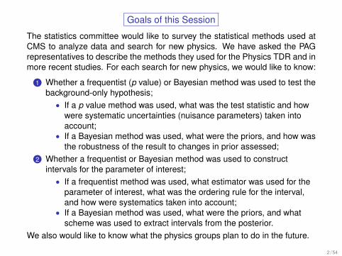
Goals of this Session

The statistics committee would like to survey the statistical methods used atCMS to analyze data and search for new physics. We have asked the PAGrepresentatives to describe the methods they used for the Physics TDR and inmore recent studies. For each search for new physics, we would like to know:

1 Whether a frequentist (p value) or Bayesian method was used to test thebackground-only hypothesis;

• If a p value method was used, what was the test statistic and howwere systematic uncertainties (nuisance parameters) taken intoaccount;

• If a Bayesian method was used, what were the priors, and how wasthe robustness of the result to changes in prior assessed;

2 Whether a frequentist or Bayesian method was used to constructintervals for the parameter of interest;

• If a frequentist method was used, what estimator was used for theparameter of interest, what was the ordering rule for the interval,and how were systematics taken into account;

• If a Bayesian method was used, what were the priors, and whatscheme was used to extract intervals from the posterior.

We also would like to know what the physics groups plan to do in the future.

2 / 54

Goals of this Talk

This talk reviews statistical methods that are applicable in HEP data analysis,with special emphasis on techniques for eliminating nuisance parameters. Thehope is that the other speakers in this session will find it useful to refer to thistalk to facilitate their own presentations.

Searches for new physics combine statistical methods for testing hypotheseswith methods for constructing intervals. The table on the next slide lists themethods we are aware of:• The column titled “technique” labels a method or class of methods;• The column titled “CLT” indicates the Z -value based notation used in the

paper by R. D. Cousins, J. T. Linnemann, and J. Tucker, “Evaluation ofthree methods for calculating statistical significance when incorporatinga systematic uncertainty into the test of the background-only hypothesisfor a Poisson process,” arXiv:physics/0702156v4 [physics.data-an] 20Nov 2008;

• The column titled “Software” lists known public routines that perform thecorresponding calculations;

• The column titled “Slide” provides clickable pointers to relevant parts ofthe talk.

3 / 54

http://xxx.lanl.gov/abs/physics/0702156

http://xxx.lanl.gov/abs/physics/0702156

Table of Methods

Purpose Technique CLT Software Slide

Hyp

othe

sis

Test

ing

• Neyman-Pearson 7

• p Values: 9

◦ Asymptotic ZPL 14

◦ Conditioning ZBi 16

◦ Supremum 17

◦ Bootstrap/plug-in 19

◦ Predictive ZN, ZΓ ScPf 22

• Bayes:◦ Hypothesis Prob. 26

◦ Bayes Factors 26

◦ Significance Testing 29

Inte

rval

Est

imat

ion • Neyman Construction TFeldmanCousins 32

◦ Marginalization 42

◦ Profiling MINOS, TRolke 42

◦ P Value Test Inversion 43

• Bayes 44

Sea

rch

Pro

-ce

dure

s • Frequentist 47

• CLS TLimit 50

• Bayes 53

4 / 54

1 Hypothesis Testing

Back to Table of Methods 5 / 54

What Do We Mean by Testing?

Two different methodologies to address two different problems:

1 We wish to decide between two hypotheses, in such a way that if we re-peat the same testing procedure many times, the rate of wrong decisionswill be fully controlled in the long run.Example: in selecting good electron candidates for a measurement of themass of the W boson, we need to minimize background contaminationand signal inefficiency. This is essentially a quality-control problem.→ Solved by Neyman-Pearson theory.

2 We wish to characterize the evidence provided by the data against agiven hypothesis.Example: in searching for new phenomena, we need to establish thatan observed enhancement of a given background spectrum is evidenceagainst the background-only hypothesis, and we need to quantify thatevidence.→ Solved by p values, likelihood ratios, or Bayes factors.


The Neyman-Pearson Theory of Testing (1)

Suppose you wish to decide which of two hypotheses, H0 or H1, is more likelyto be true given an observation X . The frequentist strategy is to minimize theprobability of making the wrong decision over many independent repetitions ofthe test procedure. However, that probability depends on which hypothesis isactually true. There are therefore two types of error that can be committed:

• Type-I error: Rejecting H0 when H0 is true;

• Type-II error: Accepting H0 when H1 is true.

To fix ideas, suppose that the hypotheses have the form:

H0 : X ∼ f0(x) versus H1 : X ∼ f1(x).

The frequentist test procedure is to specify a subset C of sample space beforelooking at the data, and to reject H0 whenever the observation falls into C. TheType-I error probability α and the Type-II error probability β are then given by:

α =

ZC

f0(x) dx and β = 1−Z

Cf1(x) dx .

The subset C is known as the critical region of the test and 1−β as its power.


The Neyman-Pearson Theory of Testing (2)

How should we choose the critical region C? The idea of the Neyman-Pearsontheory is to first select a suitably small α, and then to construct C so as tominimize β at that value of α. In the above example, the distributions f0 and f1are fully known (“simple vs. simple testing”). In this case it can be shown that,in order to minimize β at a fixed α, C must be of the form:

C = {x : f0(x)/f1(x) < cα},

where cα is a constant depending on α. This result is known as the Neyman-Pearson lemma; the quantity f0(x)/f1(x) is a likelihood ratio.

Unfortunately it is usually the case that f0 and/or f1 are composite, meaningthat they depend on one or more unknown parameters θ. The likelihood ratiois then defined as:

λ(x) ≡supθ∈H0

f0(x | θ)

supθ∈H1

f1(x | θ)

Although the Neyman-Pearson lemma does not generalize to composite tests,the likelihood ratio remains a useful test statistic, in part due to Wilks’ theorem(see later).


The p Value Method for Quantifying Evidence

Suppose we collect some data X and wish to test a hypothesis H0 about thedistribution f (x | θ) of the underlying population. A general approach is to find atest statistic T (X) such that large values of tobs ≡ T (xobs) are evidence againstthe null hypothesis H0.

A way to calibrate this evidence is to calculate the probability for observingT = tobs or a larger value under H0; this tail probability is known as the p valueof the test:

p = P(T ≥ tobs |H0).

Thus, small p values are evidence against H0. Typically one will reject H0 ifp ≤ α, where α is some predefined, small error rate. This α has essentially thesame interpretation as in the Neyman-Pearson theory, but the emphasis hereis radically different: with p values we wish to characterize post-data evidence,a concept which plays no role whatsoever in Neyman-Pearson theory.


Using p Values to Calibrate Evidence

The usefulness of p values for calibrating evidence against a null hypothesisH0 depends on their null distribution being known to the experimenter andbeing the same in all problems considered.

In principle, the very definition of a p value as a tail probability guaranteesits uniformity under H0. In practice however, it is often difficult to fulfill thisguarantee, either because the test statistic is discrete or because of the pres-ence of nuisance parameters. The following terminology characterizes the nulldistribution of p values:

p exact ⇔ P(p ≤ α |H0) = α,

p conservative ⇔ P(p ≤ α |H0) < α,

p liberal ⇔ P(p ≤ α |H0) > α.

Compared to an exact p value, a conservative p value tends to understate theevidence against H0, whereas a liberal p value tends to overstate it.


Caveats

Although the definition of p values, p ≡ P(T ≥ tobs |H0), is very simple, theircorrect interpretation is notoriously subtle. Here is partial list of caveats:

1 P values are neither frequentist error rates nor confidence levels.

2 P values are not hypothesis probabilities.

3 Equal p values do not always represent equal amounts of evidence(e.g., sample size can make a difference).

Because of these and other caveats, it is better to interpret p values as nothingmore than useful “exploratory tools,” or “measures of surprise.”

In any search for new physics, a small p value should only be seen as a firststep in the interpretation of the data, to be followed by a serious investigationof an alternative hypothesis. Only by showing that the latter provides a bet-ter explanation of the observations than the null hypothesis can one make aconvincing case for discovery.


The 5σ Discovery Threshold

A small p value has little intuitive appeal, so it is conventional to map it intothe number Nσ of standard deviations a normal variate is from zero when theprobability outside ±Nσ equals 2p :

p =

Z +∞

Nσ

dxe−x2/2

√2 π

=12

h1 − erf(Nσ/

√2)i.

The threshold for discovery is typically set at α = 2.9 × 10−7 (5σ). This con-vention dates back to the April 1968 Conference on Meson Spectroscopy inPhiladelphia, where Arthur Rosenfeld argued that, given the number of his-tograms examined by high energy physicists every year, one should expectseveral 4σ claims per year.

Why are we still using 5σ in 2009? Mainly because it still seems to work: therate of false discovery claims has not increased dramatically over the last 40years in spite of the increased rate of searches. This success is probably dueto a better understanding of detector physics (particle interactions in matter), alarger investment of CPU time in the modeling of backgrounds and systematiceffects, and the use of “safer” statistical techniques such as blind analysis.


The Problem of Nuisance Parameters

Often the distribution of the test statistic, and therefore the p value, depends onunknown “nuisance” parameters (detector energy scales, tracking efficiencies,fit parameters, etc.). In HEP there are essentially five classes of methods foreliminating nuisance parameters:

1 Asymptotic;

2 Structural;

3 Supremum;

4 Bootstrap;

5 Predictive.

The first four methods are compatible with a frequentist definition of probability,but only 2 and 3 guarantee a conservative p value. The last method requiresa Bayesian concept of probability.


Asymptotic Methods (1)

Some test statistics have an asymptotic distribution that is independent of anyunknown parameters. These distributions can be used to approximate p val-ues in finite, but large enough samples. Suppose for example that we aretesting H0 : θ ∈ Θ0 versus H1 : θ ∈ Θ \ Θ0. The likelihood ratio statistic canthen be defined as:

λ(x) ≡supΘ0

L(θ | x)

supΘL(θ | x)

=L(θ̂0 | x)

L(θ̂ | x),

where θ̂0 is the maximum likelihood estimate (MLE) under H0 and θ̂ is theunrestricted MLE. Note that 0 ≤ λ(x) ≤ 1.

A likelihood ratio test is a test whose rejection region has the form {x : λ(x) ≤c}, where c is a constant between 0 and 1.

To calculate p values based on λ(X ) we need the distribution of λ(X ) underH0:

[Wilks’ Theorem] Under suitable regularity conditions the asymptotic distribu-tion of −2 ln λ(X ) under H0 is chisquared with ν − ν0 degrees of freedom,where ν = dim Θ and ν0 = dim Θ0.


Asymptotic Methods (2)

It is not uncommon in HEP for one or more regularity conditions to be violated:

1 The tested hypotheses must be nested, i.e. H0 must be obtainable byimposing parameter restrictions on the model that describes H1.As counter-example consider a test comparing two new-physics modelsthat belong to separate families of distributions.

2 H0 must not be on the boundary of the model that describes H1.A typical violation of this condition is when θ is a positive signalmagnitude and one is testing H0 : θ = 0 versus H1 : θ > 0.

3 There must not be any nuisance parameters that are defined under H1

but not under H0.Suppose that we are searching for a signal peak on top of a smoothbackground. The location, width, and amplitude of the peak areunknown. In this case the location and width of the peak are undefinedunder H0, so the likelihood ratio will not have a chisquared distribution.This is the look-elsewhere effect.

There does exist analytical work on the distribution of −2 ln λ(X ) when theabove regularity conditions are violated; however these results are not alwayseasy to apply and still require some numerical calculations. Physicists usuallyprefer to simulate the −2 ln λ(X ) distribution from scratch.


Structural Methods

These are methods that require the testing problem to have a special struc-ture in order to eliminate nuisance parameters. An interesting example is theconditioning method, where one has some data D and there exists a statis-tic C = C(D) such that the distribution of D given C is independent of thenuisance parameter(s) under the null hypothesis. Then one can use that con-ditional distribution to calculate p values. For example, suppose we observe:

N ∼ Poisson(µ + ν) and M ∼ Poisson(τν),

where µ is the parameter of interest, ν a nuisance parameter, and τ a knownconstant. The distribution of N given C ≡ N +M is binomial under H0, and thep value for the observation N = n0 and conditional on C = n0 + m0, is:

pcond =

n0+m0Xn=n0

n0 + m0

n

!„1

1 + τ

«n „1− 1

1 + τ

«n0+m0−n

This method is sometimes used to evaluate the significance of a bump in apredefined signal window in a smooth spectrum, when the background in thewindow can be estimated from “sidebands”.


Supremum Methods (1)

Structural methods have limited applicability due to their requirement of the ex-istence of a special structure in the testing problem. A very general techniqueconsists in maximizing the p value with respect to the nuisance parameter(s):

psup = supν

p(ν).

This is essentially a “worst case” analysis. Psup is guaranteed to be conser-vative, but may yield the trivial result psup = 1 if one is not careful in the choiceof test statistic. In general the likelihood ratio λ is a good choice.

A great simplification occurs when −2 ln λ is stochastically increasing† with ν,because then psup = p∞ ≡ limν→∞ p(ν), and, under some regularity con-ditions p∞ is a chisquared tail probability by Wilks’ theorem. Unfortunatelystochastic monotonicity is not generally true, and is often difficult to check.When psup 6= p∞, p∞ will tend to be liberal.

† A statistic T is stochastically increasing with the parameter ν if ν1 > ν2

implies F (T | ν1) ≤ F (T | ν2) for all T and F (T | ν1) < F (T | ν2) for some T ,where F (T | ν) is the cumulative distribution of T . In other words, the randomvariable T tends to be larger if ν increases.


Supremum Methods (2)

The supremum method has two important drawbacks:

1 Computationally, it is often difficult to locate the global maximum of therelevant tail probability over the entire range of the nuisance parameterν.

2 Conceptually, the very data one is analyzing often contain informationabout the true value of ν, so that it makes little sense to maximize overall values of ν.

A simple way around these drawbacks is to maximize over a 1− γ confidenceset Cγ for ν, and then to correct the p value for the fact that γ is not zero:

pγ = supν∈Cγ

p(ν) + γ.

Here the supremum is restricted to all values of ν that lie in the confidence setCγ . It can be shown that pγ , like psup, is conservative:

P(pγ ≤ α) ≤ α for all α ∈ [0, 1].

pγ is known as a confidence interval p value.


Bootstrap Methods (1)The simplest bootstrap method is the plug-in: it eliminates unknown param-eters by estimating them under the null hypothesis, using for example themaximum-likelihood method, and then substituting the estimate in the calcu-lation of the p value.

Suppose that we measure N ∼ Poisson(µ + ν), where µ is a signal rateand ν a background rate constrained by an auxiliary measurement of X ∼Gauss(ν, ∆ν), and that we wish to test H0 : µ = 0. The likelihood function is:

L(µ, ν | x , n) =(µ + ν)n e−µ−ν

n!

e− 1

2

„x−ν∆ν

«2

√2π ∆ν

.

The maximum-likelihood estimate of ν under H0 is obtained by setting µ = 0and solving ∂ lnL/∂ν = 0 for ν. This yields:

ν̂(x , n) =x −∆ν2

2+

s„x −∆ν2

2

«2

+ n ∆ν2.

Using N as test statistic, the plug-in p value is then:

pplug(x , n) ≡ PhN ≥ n

˛̨̨ν = ν̂(x , n)

i=

+∞Xk=n

ν̂(x , n)k e−ν̂(x,n)

k !.


Bootstrap Methods (2)

Two criticisms can be leveled at the plug-in method. First, it makes doubleuse of the data, once to estimate the nuisance parameters under H0, and thenagain to calculate a p value. Second, it does not take into account the un-certainty on the parameter estimates. The net effect is that plug-in p valuestend to be too conservative. It is possible to compensate for this overcon-servativeness by bootstrapping the plug-in p value (see next slide). This is adouble bootstrap known as the adjusted plug-in p value. Unfortunately double-bootstrapping is very CPU intensive.

In HEP the plug-in method is typically used when the test statistic T is theresult of a complicated fit to signal plus background, for example when T is theamplitude of a resonance of unknown location in an invariant mass spectrum.To evaluate the significance one has to repeat the fit on a large number oftoy experiments; the parameters needed to generate these experiments aredetermined from a fit to the actual data under the null hypothesis and then“plugged into” the generation mechanism.


Bootstrap Methods (3)

The double-bootstrap procedure works as follows:1 Use the actual data to obtain the test statistic t0 and whatever parameter

estimates are needed to generate toy experiments under the nullhypothesis H0.

2 Generate B1 first-level bootstrap samples (i.e. toy experiments) underH0, and use each of them to compute a bootstrap test statistic t?

j ,j = 1, . . . , B1.

3 Use t0 and the t?j to calculate the first-level bootstrap (i.e., plug-in) p

value p?0 ≡ #{t?

j : t?j ≥ t0}/B1.

4 For each of the B1 first-level bootstrap samples, generate B2

second-level bootstrap samples, and use each of them to compute asecond-level bootstrap test statistic t??

j` for ` = 1, . . . , B2.5 For each of the B1 first-level bootstrap samples, compute the

second-level bootstrap p value p??j ≡ #{t??

j` : t??j` ≥ t?

j , j given}/B2.6 Compute the double-bootstrap p value as the proportion of the p??

j thatare smaller (i.e. more extreme) than p?

0 : p??0 ≡ #{p??

j : p??j < p?

0}/B1.Notes: (1) Double bootstrapping should only be used when the test statistic isasymptotically pivotal; (2) double bootstrap tests are not guaranteed to alwayswork well; (3) there exist faster versions of the above algorithm.


Predictive Methods (1)

Suppose we have a proper Bayesian prior π(θ) for all the unknown param-eters θ in the problem. Given a test statistic T , we can then construct theprior-predictive distribution of T , i.e. the predicted distribution of T before themeasurement:

mprior (t) =

Zdθ p(t | θ) π(θ).

After having observed T = t0 we can quantify how surprising this observationis by referring t0 to mprior , e.g. by calculating the prior-predictive p value:

pprior = Pmprior (T ≥ t0 |H0) =

Z ∞

t0

dt mprior (t)

=

Zdθ π(θ)

"Z ∞

t0

dt p(t | θ)

#= Eπ

hpθ

i,

where pθ is the usual p value evaluated at a fixed θ and Eπ is the expectationwith respect to the prior π(θ). Note that mprior (t) is not a proper distribution ifthe prior π(θ) is improper. In this case it will not be possible to define a prior-predictive p value; a posterior-predictive method might work however (see nextslide).



The posterior-predictive distribution of a test statistic T is the predicted distri-bution of T after measuring T = t0:

mpost(t | t0) =

Zdθ p(t | θ) π(θ | t0)

The posterior-predictive p value estimates the probability that a future obser-vation will be at least as extreme as the current observation if the null hypoth-esis is true:

ppost = Pmpost (T ≥ t0 |H0) =

Z ∞

t0

dt mpost(t | t0)

=

Zdθ π(θ | t0)

"Z ∞

t0

dt p(t | θ)

#= Eπ(· | t0)

hpθ

i.

Note the double use of the observation t0.

In contrast with prior-predictive p values, posterior-predictive p values can of-ten be defined when the prior is improper.



The prior-predictive p value is a very natural method to use when informationabout the nuisance parameter does not come (only) from a subsidiary mea-surement but includes results from Monte Carlo studies, theoretical beliefs,etc. In that case the p value represents a tail probability in an ensemble thatincorporates variations in our subjective information about the nuisance pa-rameter and is not purely frequentist. The prior-predictive ensemble consistsin fluctuating parameter values in the toy experiments, and generating datafrom the fluctuated values of the parameters; it is quite common in HEP.

It sometimes happens that one has no or very little prior information about anuisance parameter, for example the magnitude of a multijet QCD background.In that case it is not possible to construct a proper prior for the nuisance param-eter, and the prior-predictive method will not work. However, the data sampleitself may provide information about the nuisance parameter, so that one willbe able to construct a posterior-predictive p value.

When a proper nuisance prior is available, the posterior-predictive methodtends to be much more conservative than the prior-predictive one, due to theformer’s double use of the data.


Further Comments on P Value Methods

We have described five classes of methods for eliminating nuisance parame-ters in p value calculations: asymptotic, structural, supremum, bootstrap, andpredictive. Here are some additional comments:

• For a fixed observation, a p value should increase as the uncertainty onthe nuisance parameter increases. This is generally true of the methodswe have surveyed, but there is no theorem that guarantees this.

• It is sometimes interesting to check the result of more than one p valuemethod. In large data samples some methods will give nearly identicalresults.

• In principle p values should be uniformly distributed under H0, but inpractice they can deviate quite a bit from uniformity. This also dependson the choice of test statistic. One should of course check this, keepingin mind that “conservatism” is preferable to “liberalism”.

• The power of the various p values to detect an interesting effectdepends on the choice of test statistic.

• Due to their Bayesian nature, the predictive p values can be calculatedfor discrepancy variables (i.e. functions of both data and parameters,such as a sum of squared residuals) in addition to test statistics.


Bayesian Hypothesis Testing (1)

The Bayesian approach to hypothesis testing is to calculate posterior proba-bilities for all hypotheses in play. When testing H0 versus H1, Bayes’ theoremyields:

π(H0 | x) =p(x |H0) π0

p(x |H0) π0 + p(x |H1) π1,

π(H1 | x) = 1 − π(H0 | x),

where πi is the prior probability of Hi , i = 0, 1.

If π(H0 | x) < π(H1 | x), one rejects H0 and the posterior probability of erroris π(H0 | x). Otherwise H0 is accepted and the posterior error probability isπ(H1 | x).

In contrast with frequentist Type-I and Type-II errors, Bayesian error probabil-ities are fully conditioned on the observed data. It is often interesting to lookat the evidence against H0 provided by the data alone. This can be done bycomputing the ratio of posterior odds to prior odds and is known as the Bayesfactor:

B01(x) =π(H0 | x)/π(H1 | x)

π0/π1

In the absence of unknown parameters, B01(x) is a likelihood ratio.Back to Table of Methods 26 / 54


Often the distributions of X under H0 and H1 will depend on unknown parame-ters θ, so that posterior hypothesis probabilities and Bayes factors will involvemarginalization integrals over θ:

π(H0 | x) =

Zp(x | θ, H0) π(θ |H0) π0 dθZ h

p(x | θ, H0) π(θ |H0) π0 + p(x | θ, H1) π(θ |H1) π1

idθ

and: B01(x) =

Zp(x | θ, H0) π(θ |H0) dθZp(x | θ, H1) π(θ |H1) dθ

Suppose now that we are testing H0 : θ = θ0 versus H1 : θ > θ0. Then:

B01(x) =p(x | θ0)Z

p(x | θ, H1) π(θ |H1) dθ

≥ p(x | θ0)

p(x | θ̂1)= λ(x).

The ratio between the Bayes factor and the corresponding likelihood ratio islarger than 1, and is sometimes called the Ockham’s razor penalty factor: itpenalizes the evidence against H0 for the introduction of an additional degreeof freedom under H1, namely θ.



Small values of B01, or equivalently large values of B10 ≡ 1/B01, are evidenceagainst the null hypothesis H0. A rough descriptive statement of standards ofevidence provided by Bayes factors against a given hypothesis is as follows:

2 ln B10 B10 Evidence against H0

0 to 2 1 to 3 Not worth more than a bare mention2 to 6 3 to 20 Positive6 to 10 20 to 150 Strong> 10 > 150 Very strong

(See R.E. Kass and A.E. Raftery, “Bayes Factors,” J. Amer. Statist. Assoc. 90,773 (1995).)

In HEP we do not have much experience with Bayes factors, so the aboveinterpretations should be taken with some caution.


Bayesian Significance Tests

For a hypothesis of the form H0 : θ = θ0, a test can be based directly onthe posterior distribution of θ. First calculate an interval for θ, containing anintegrated posterior probability β. Then, if θ0 is outside that interval, reject H0

at the α = 1 − β credibility level. An exact significance level can be obtainedby finding the smallest α for which H0 is rejected.

There is a lot of freedom in the choice of posterior interval. A natural pos-sibility is to construct a highest posterior density (HPD) interval. If the lackof parametrization invariance of HPD intervals is a problem, there are otherchoices. One is to use a standard ∆ lnL interval subject to the constraint ofa given posterior credibility content (see slides on Bayesian interval construc-tions later on).

If the null hypothesis is H0 : θ ≤ θ0, a valid approach is to calculate a lowerlimit θL on θ and exclude H0 if θ0 < θL. In this case the exact significance levelis the posterior probability of θ ≤ θ0.


2 Constructing Interval Estimates


What Are Interval Estimates?Suppose that we make an observation X = xobs from a distribution f (x |µ),where µ is a parameter of interest, and that we wish to make a statementabout the true value of µ, based on our observation xobs. One possibility is tocalculate a point estimate µ̂ of µ, f.e. via the maximum-likelihood method:

µ̂ = arg maxµ

f (xobs |µ).

Although such a point estimate has its uses, it comes with no measure ofhow confident we can be that the true value of µ equals µ̂. Bayesianism andFrequentism both address this problem by constructing an interval of µ valuesbelieved to contain the true value with some confidence. However, the intervalconstruction method and the meaning of the associated confidence level arevery different in the two paradigms:• Frequentists build an interval [µ1, µ2] whose boundaries µ1 and µ2 are

random variables that depend on X in such a way that if themeasurement is repeated many times, a fraction γ of the producedintervals will cover the true µ; the fraction γ is called the confidence levelor coverage of the interval construction.

• Bayesians construct the posterior probability density of µ and choosetwo values µ1 and µ2 such that the integrated posterior probabilitybetween them equals a desired level γ, called credibility or Bayesianconfidence level of the interval.


Frequentist Intervals: the Neyman Construction (1)

Step 1: Make a graph of the parameter µ versus the data X , and plot thedensity distribution of X for each value of µ.



Step 2: For each value of µ, select an interval of X values that has a fixedintegrated probability, for example 68%.



Step 3: Connect the interval boundaries across µ values.



Step 4: Drop the “scaffolding” and use the resulting confidence belt toconstruct an interval [µ1, µ2] for the true value of µ every time you make anobservation xobs of X .



Why does this work? Suppose µ? is the true value of µ. ThenP(x1 ≤ X ≤ x2 |µ?) = 68%. Furthermore, for every X ∈ [x1, x2], the reportedµ-interval contains µ?, and for every X 6∈ [x1, x2], the reported interval doesnot contain µ?. Therefore, the probability of covering µ? is 68%.


The Neyman Construction: Ingredients (1)

There are four basic ingredients in the frequentist interval construction: anestimator µ̂ of the parameter of interest µ, an ordering rule, a reference en-semble, and a confidence level. Let’s look at each of these in turn.

1. The choice of estimatorThis is best understood with the help of an example. Suppose we collect nmeasurements xi of the mean µ of a Gaussian distribution with known width.Then clearly we should use the average x̄ of the xi as an estimate of µ, sincex̄ is a sufficient statistic† for µ. Hence it makes sense to plot x̄ along thehorizontal axis in the Neyman construction.

Suppose now that µ is constrained to be positive. Then we could use µ̂ = x̄or µ̂ = max{0, x̄}. These two estimators lead to intervals with very differentproperties.

† A statistic T (X ) is sufficient for µ if the conditional distribution of the sampleX given T (X ) does not depend on µ. In this sense, T (X ) captures all theinformation about µ contained in the sample.



2. The choice of ordering ruleAt step 2 of the Neyman construction, the rule used to select which x valuesto include in the x-interval for a given µ is known as an ordering rule. Order-ing rules should be chosen consistently for all parameter values: this is whatgives frequentist intervals their inferential meaning. Thus it is also possible toview ordering rules as ordering parameter values according to their perceivedcompatibility with the observed data. Here are some examples, all assumingthat we have observed data x and are interested in a 68% confidence interval[µ1, µ2] for a parameter µ whose maximum likelihood estimate is µ̂(x):• Central ordering

[µ1, µ2] is the set of µ values for which x falls between the 16th and 84th

percentiles of its distribution.• Probability density ordering

[µ1, µ2] is the set of µ values for which x falls within the 68% mostprobable region of its distribution.

• Likelihood ratio ordering[µ1, µ2] is the set of µ values for which the observed data falls within a68% probability region R, such that any point inside R has a largerlikelihood ratio L(µ)/L(µ̂(x)) than any point outside R.



2. The choice of ordering rule (continued)

• Upper limit ordering]−∞, µ2] is the set of µ values for which x is at least as large as the32nd percentile of its distribution.

• Lower limit ordering]µ1, +∞] is the set of µ values for which x is at most as large as the 68th

percentile of its distribution.



3. The choice of reference ensembleThis refers to the replications of a measurement that are used to calculate cov-erage. In order to specify these replications, one must decide which randomand non-random aspects of the measurement are relevant to the inference ofinterest.

Example: when measuring the mass of a short-lived particle, it may be thatits decay mode affects the measurement resolution. Should we then refer ourmeasurement to an ensemble that includes all possible decay modes, or onlythe decay mode actually observed?

By using the unconditional ensemble (all possible decay modes), one canobtain shorter intervals. However, in this case most people would agree thatconditioning on the decay mode is more “relevant” and is the right thing to do.



4. The choice of confidence levelThe confidence level labels a family of intervals; some conventional values are68%, 90%, and 95%. It is very important to remember that a confidence leveldoes not characterize single intervals; it only characterizes families of inter-vals. For example, suppose we are interested in the mean µ of a Gaussianpopulation with unit variance. We have two observations, x and y , so that themaximum likelihood estimate of µ is µ̂ = (x +y)/2. Consider the following twointervals for µ:

I1 : µ̂± 1/√

2 and I2 : µ̂±q

max{0, 4.60− (x − y)2/4}.

Both I1 and I2 are centered on the maximum likelihood estimate of µ. IntervalI1 uses likelihood ratio ordering, is never empty, and has 68% coverage. Inter-val I2 uses probability density ordering, is empty whenever |x−y | ≥ 4.29, andhas 99% coverage. Suppose now that we observe x = 10.00 and y = 14.05.It is easy to verify that the corresponding I1 and I2 intervals are numericallyidentical and equal to 12.03± 0.71.

Thus, the same numerical interval can have two very different coverages, de-pending on which ensemble it is considered to belong to.


The Neyman Construction: Nuisance Parameters (1)

The Neyman construction can be performed when there is more than oneparameter; it becomes multi-dimensional and the confidence belt becomes a“hyperbelt”. Nuisance parameters can be eliminated by projecting the finalconfidence region onto the parameter(s) of interest at the end of the construc-tion. The difficulty is to design the ordering rule so as to minimize the amountof overcoverage introduced by projecting. Simpler solutions include:

1 Marginalizing: Eliminate the nuisance parameters by integrating thedata pdf over proper prior distributions (this is a Bayesian step):

f (x |µ, ν) → f̃ (x |µ) ≡Z

f (x |µ, ν) π(ν) dν.

The resulting data pdf depends only on the parameter(s) of interest andcan be used in a standard Neyman construction.

2 Profiling: Eliminate the nuisance parameters by maximizing the pdf:

f (x |µ, ν) → f̆ (x |µ) ∝ maxν

nf (x |µ, ν)

o= f (x |µ, ˆ̂ν(µ)).

The profiled pdf is then used in a standard Neyman construction.

Note: the frequentist coverage of the simpler solutions is not guaranteed!


The Neyman Construction: Nuisance Parameters (2)

A different way of looking at the Neyman construction is via test inversion.Suppose we are interested in some parameter θ ∈ Θ. If for each allowedvalue θ0 of θ we can construct an exact p value to test H0 : θ = θ0, then wecan also construct one- and two-sided γ confidence-level intervals for θ:

C1γ =n

θ : pθ ≥ 1− γo

and C2γ =n

θ :1− γ

2≤ pθ ≤

1 + γ

2

o,

where we explicitly indicated the θ dependence of the p value. In words: aγ confidence limit for θ is obtained by collecting all the θ values that are notrejected at the 1−γ significance level by the p value test. To see this, considerthe one-sided case:

P[θtrue ∈ C1γ ] = P[pθtrue ≥ 1−γ] = 1−P[pθtrue < 1−γ] = 1− (1−γ) = γ.

Now, if the testing problem involves nuisance parameters, and we can elim-inate these from pθ for each θ, then we can also construct nuisance-free in-tervals for θ. Furthermore, if the p value test is unbiased, the correspondingconfidence interval will also be unbiased.


Bayesian Interval Constructions (1)

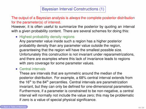
The output of a Bayesian analysis is always the complete posterior distributionfor the parameter(s) of interest.However, it is often useful to summarize the posterior by quoting an intervalwith a given probability content. There are several schemes for doing this:• Highest probability density regions

Any parameter value inside such a region has a higher posteriorprobability density than any parameter value outside the region,guaranteeing that the region will have the smallest possible size.Unfortunately this construction is not invariant under reparametrizations,and there are examples where this lack of invariance leads to regionswith zero coverage for some parameter values.

• Central intervalsThese are intervals that are symmetric around the median of theposterior distribution. For example, a 68% central interval extends fromthe 16th to the 84th percentiles. Central intervals are parametrizationinvariant, but they can only be defined for one-dimensional parameters.Furthermore, if a parameter is constrained to be non-negative, a centralinterval will normally not include the value zero; this may be problematicif zero is a value of special physical significance.


Bayesian Interval Constructions (2)

• Upper and lower limitsFor one-dimensional posterior distributions, these one-sided intervalscan be defined using percentiles.

• Likelihood regionsThese are standard likelihood regions where the likelihood ratio betweenthe region boundary and the likelihood maximum is adjusted to obtainthe desired posterior credibility. Such regions are metric independentand robust with respect to the choice of prior. In one-dimensionalproblems with physical boundaries, these regions smoothly transitionfrom one-sided to two-sided intervals.

• Intrinsic credible regionsThese are intervals of parameter values with minimum referenceposterior expected loss (a concept from Bayesian reference analysis).

Some things to watch for when quoting Bayesian intervals:

• How sensitive are the intervals to the choice of prior?

• Do the intervals have reasonable coverage?


3 Search Procedures


Frequentist Search ProceduresSearch procedures combine techniques from hypothesis testing and intervalconstruction. The standard frequentist procedure to search for new physicsprocesses is as follows:

1 Calculate a p value to test the null hypothesis that the data weregenerated by standard model processes alone.

2 If p ≤ α1 claim discovery and calculate a two-sided, α2 confidence levelinterval on the production cross section of the new process.

3 If p > α1 calculate an α3 confidence level upper limit on the productioncross section of the new process.

Typical confidence levels are α1 = 2.9× 10−7, α2 = 0.68, and α3 = 0.95.

There are a couple of issues regarding this procedure:• Coverage

The procedure involves one p value and two confidence intervals; whatis the proper reference ensemble for each of these objects?

• SensitivityThe purpose of reporting an upper limit when failing to claim a discoveryis to exclude cross sections that the experiment is sensitive to and didnot detect. How to avoid excluding cross sections that the experiment isnot sensitive to?


Frequentist Search Procedures: the Coverage Issue

The usual HEP approach to interval/upper limit construction after a test is todo the construction as if no test had preceded it, i.e. unconditionally. Froma frequentist point of view this is incorrect: the upper limit will undercover forlarge values of the new process cross section, and the two-sided interval willundercover for small values. There will be undercoverage even if we set α2 =α3, because this corresponds to “flip-flopping”, selecting the ordering rule afterlooking at the data. Finally, the unconditional approach is also problematicbecause it uses the same data twice, first for the hypothesis test, and thenagain for the interval construction.

The solution is to construct intervals by conditioning on the result of the test.If the background-only hypothesis is rejected, the two-sided interval shouldbe constructed after restricting the sample space to the critical region of thetest and renormalizing the pdf accordingly. Similarly, if the background-onlyhypothesis is accepted, the upper limit should be constructed after restrictingthe sample space to the region outside the critical region and renormalizingthe pdf accordingly.

In practice however, the conditional construction only differs from the uncondi-tional one when the data is in the vicinity of the discovery threshold.


Frequentist Search Procedures: the Sensitivity Issue (1)

Suppose the result of a test of H0 is that it can’t be rejected: we find p0 > α1,where the subscript 0 on the p value emphasizes that it is calculated underthe null hypothesis. A natural question is then: what values of the new physicscross section µ can we actually exclude? This is answered by calculating anα3 C.L. upper limit on that cross section, and the easiest way to do this is byinverting a p value test: exclude all µ values for which p1(µ) ≤ 1 − α3, wherep1(µ) is the p value under the alternative hypothesis that µ > 0.

If our measurement has no sensitivity for a particular value of µ, this meansthat the distribution of the test statistic is (almost) the same under H0 and H1.In this case p0 ∼ 1− p1, and under H0 we have:

P0(p1 ≤ 1−α3) ∼ P0(1−p0 ≤ 1−α3) = P0(p0 ≥ α3) = 1−P0(p0 < α3) = 1−α3.

For example, if we calculate a 95% C.L. upper limit, there will be a∼ 5% prob-ability that we will be able to exclude µ values for which we have no sensitivity.


CLS

Some experimentalists consider that a 5% probability of excluding values ofthe parameter µ to which the experiment is not sensitive is too much; to avoidthis problem they only exclude µ values for which

p1(µ)

1− p0≤ 1− α3.

The left-hand side is known as CLS. The resulting procedure overcovers. Notethat even though the name CLS contains the initials for Confidence Level, thecorresponding quantity is just a ratio of p values, not a confidence level.

Important: there is no such thing as “the” CLS method, because users of theCLS quantity differ in their handling of nuisance parameters: some use profil-ing, others marginalization. One should always report how the calculation wasdone in this respect.



Plot of contours of equal measurement resolution in the p1 versus p0 plane.Since p1 ≡ F1(x) and p0 ≡ 1− F0(x), we have p1 = F1[F−1

0 (1− p0)].



An interesting way to quantify a priori the sensitivity of a test, when the newphysics model depends on a parameter µ, is to report the set of µ values forwhich

1− β(α1, µ) ≥ α3.

This µ sensitivity region has a couple of valuable interpretations:

1 If the true value of µ is in the sensitivity region, the probability of makinga discovery is at least α3, by definition of β.

2 If the test does not result in discovery, it will be possible to exclude atleast the entire sensitivity region with confidence α3. Indeed, if we fail toreject H0 at the α1 level, then we can reject any µ in H1 at the β(α1, µ)level, so that p1(µ) ≤ β(α1, µ); furthermore, if µ is in the sensitivityregion, then β(α1, µ) ≤ 1− α3 and therefore p1(µ) ≤ 1− α3, meaningthat µ is excluded with confidence α3.

In general the sensitivity region depends on the event selection and the choiceof test statistic. Maximizing the former provides a criterion for optimizing thelatter. The appeal of this criterion is that it optimizes the result regardless ofthe outcome of the test.


Bayesian Search Procedures (1)The starting point of a Bayesian search is the calculation of a Bayes factor.For a test of the form H0 : θ = θ0 versus H1 : θ > θ0, this can be written as:

B01(x) =p(x | θ0)Z

p(x | θ, H1) π(θ |H1) dθ

,

and points to an immediate problem: what is an appropriate prior π(θ |H1) forθ under the alternative hypothesis?

Ideally one would be able to elicit some kind of proper “consensus” prior rep-resenting scientific knowledge prior to the experiment.

If this is not possible, one might want to use an “off the shelf” objective prior,but such priors are typically improper, and therefore only defined up to a mul-tiplicative constant, rendering the Bayes factor useless. Methods exist to con-vert improper objective priors into proper objective priors suitable for testingproblems, but the conversion is often computationally demanding. . .

An alternative to the construction of a proper prior for this problem is to reportthe minimum Bayes factor in favor of H0, i.e. B01 min ≡ minθ[p(x | θ0)/p(x | θ, H1)].Although some care is required to interpret this quantity correctly, in many re-spects it provides an improvement over p values.


Bayesian Search Procedures (2)

In addition to the Bayes factor we need prior probabilities for the hypothesesthemselves. An “objective” choice is the impartial π(H0) = π(H1) = 1/2. Theposterior probability of H0 is then

π(H0 | x) =B01

1 + B01.

The complete outcome of the search is then:

• The posterior probability of the null hypothesis, π(H0 | x);

• The posterior distribution of θ under the alternative hypothesis,π(θ | x , H1).

The posterior distribution of H1 can be summarized by calculating an upperlimit or a two-sided interval.


The Rockefeller Universityphysics.rockefeller.edu/luc/talks/SearchProcedures.pdfSearch Procedures...

Documents

Transcript of The Rockefeller Universityphysics.rockefeller.edu/luc/talks/SearchProcedures.pdfSearch Procedures...