HAL Id: halshs-00588318https://halshs.archives-ouvertes.fr/halshs-00588318

Preprint submitted on 26 Apr 2011

HAL is a multi-disciplinary open accessarchive for the deposit and dissemination of sci-entific research documents, whether they are pub-lished or not. The documents may come fromteaching and research institutions in France orabroad, or from public or private research centers.

L’archive ouverte pluridisciplinaire HAL, estdestinée au dépôt et à la diffusion de documentsscientifiques de niveau recherche, publiés ou non,émanant des établissements d’enseignement et derecherche français ou étrangers, des laboratoirespublics ou privés.

The Rich in Argentina over the twentieth century: Fromthe Conservative Republic to the Peronist experience

and beyond 1932-2004Facundo Alvaredo

To cite this version:Facundo Alvaredo. The Rich in Argentina over the twentieth century: From the Conservative Republicto the Peronist experience and beyond 1932-2004. 2007. �halshs-00588318�

WORKING PAPER N° 2007 - 02

The rich in Argentina over the twentieth century:

From the conservative republic to the Peronist experience

and beyond 1932-2004

Facundo Alvaredo

JEL Codes: D3, H2, N3, O1 Keywords: income distribution, top incomes, taxation

PARIS-JOURDAN SCIENCES ECONOMIQUES

LABORATOIRE D’ECONOMIE APPLIQUÉE - INRA

48, BD JOURDAN – E.N.S. – 75014 PARIS TÉL. : 33(0) 1 43 13 63 00 – FAX : 33 (0) 1 43 13 63 10

www.pse.ens.fr

CENTRE NATIONAL DE LA RECHERCHE SCIENTIFIQUE – ÉCOLE DES HAUTES ÉTUDES EN SCIENCES SOCIALES ÉCOLE NATIONALE DES PONTS ET CHAUSSÉES – ÉCOLE NORMALE SUPÉRIEURE

This version: October 2007

The Rich in Argentina during the Twentieth Century From the Conservative Republic to the Peronist Experience and beyond

1932-2004*

Facundo AlvaredoΨ

Paris School of Economics and CREST

Abstract

This paper presents series of top income shares in Argentina from 1932 to 2004

based on personal income tax return statistics. The results suggest that income

concentration was higher during the 1930s and the first half of the 1940s than it

is today. The recovery of the economy after the Great Depression, favored by the

international trade conditions during and after the Second World War, and the

visible effects of the Peronist policy between 1945 and 1955 generated an

inverted U shape in the dynamics of top incomes. There is evidence suggesting

the limits of the Peronist redistributive policy: by 1956 the top income shares

were still far from the ones observed in the developed world. Since then, and

after a new upward movement between 1956 and 1959, the top shares seem to

have described the U-shape pattern found in English-speaking economies.

JEL classification: D3, H2, N3, O1

* I am grateful to Hildegart Ahumada, Tony Atkinson, Heber Camelo, Alfredo Canavese, Rafael Di Tella, Leonardo Gasparini, Daniel Heymann, Emmanuel Saez, José Antonio Sánchez Román, Walter Sosa Escudero and Analía Vasallo, as well as many seminar participants at PSE (Paris) and the 2006 World Bank Network of Income and Poverty Meeting for helpful comments. Special thanks go to Thomas Piketty for encouraging the work on Argentina. Ψ Paris School of Economics, Ecole Normale Supérieure, 48 Boulevard Jourdan, 75014 Paris. Email: alvaredo @ pse.ens.fr.

2

1.Introduction

This paper presents series of top income shares in Argentina between 1932 and

2004. The use of statistical information from the Argentine personal income tax,

never exploited before, allows us to cover a long span and fill a gap in the

analysis of the long run dynamics of income concentration. We find an increase

in top income shares after the Great Depression, with maxima in 1942-1943, and

a substantial decline during the Peronist years. However, the limits of the

Peronist redistributive policy are marked by the fact that in 1956, if lower than in

1945, the top shares were still far from the ones observed in the developed

world; they were higher than in the US and much higher than in France, for

instance. Since then, and after a new upward movement between 1956 and

1959, top shares seem to have described the U-shape pattern found in the

developed English-speaking economies.

The evolution of the dynamics of top incomes has attracted much attention lately.

The book recently edited by Atkinson and Piketty (2007) is an example of this

interest. The countries studied in the volume are Anglo-Saxon (United Kingdom,

Ireland, United States, Canada, New Zealand and Australia) and continental

European countries (France, Germany, Netherlands, and Switzerland).1 The

authors found a drop in income concentration in the first part of the twentieth

century (mainly between the Great Depression and the end of the Second World

War) that was essentially the result of a fall in top capital incomes due to

destruction, inflation, bankruptcies and fiscal policies to finance war debts.2 The

reason why capital incomes did not recover during the second half of the century

is still an open question; Piketty (2003) and Piketty and Saez (2006) suggest that

the introduction of generalized progressive income and estate taxation made

1 Atkinson (2005), Atkinson and Leigh (2007 a,b), Dell (2007), Dell et al. (2007), Kopczuk and Saez (2004), Nolan (2007), Piketty et al. (2006), Piketty (1998), Piketty and Saez (2003), Saez and Veall (2005), Salverda and Atkinson (2007). 2 The timing and the magnitude of the decline vary across countries.

3

such a reversal impossible.3 The last thirty years tell a different story. The United

States, Canada and the United Kingdom have displayed a substantial increase in

top shares driven by large increases in top wages, whereas this phenomenon did

not happen in continental Europe or Japan. Research has also been done on the

experiences of Spain, India, Portugal, Japan, Ireland, Sweden, Norway, China

and Indonesia.4

The case of Argentina is unique and consequently worth studying on several

grounds.

1. So far, Banerjee and Piketty (2005) on India, Piketty and Qian (2006) on

China, Leigh and van der Eng (2007) on Indonesia, and this paper on Argentina

are the only works providing evidence for –currently– developing countries.

Argentina is the first case to be analyzed in Latin America.

2. Secondly, Argentina was once a relatively rich country that has consistently

diverged from the industrial economies in the last fifty years; today it is

indistinguishably a middle income emerging economy. The deterioration of the

country’s position is one of the puzzling cases in the economics of development.

Between 1880 and 1930, the economy displayed a growth process that changed

its marginal position in the world and made many think that the country would

play in South America the role the United States stood for in the north.5 It

enjoyed its own Belle Époque between 1900 and 1913. The formula of success

3 In fact, Switzerland stayed neutral during wars and never implemented very progressive personal taxation schemes; top wealth shares were much more stable (see Dell et al. (2006)). According to Nolan (2007), Ireland did not experience a significant drop in top income shares during the Second World War, them being rather similar in 1920 and 1950; nevertheless, they sharply declined in post war decades in parallel with the enforcement of progressive taxation with very high top marginal rates. 4 Alvaredo (2007), Alvaredo and Saez (2006), Banerjee and Piketty (2005), Leigh and van der Eng (2007), Moriguchi and Saez (2007), Piketty and Qian (2006). 5 To make reference to one of the multiple examples of this optimism, both the First Bank of Boston and the City of New York Bank (Citibank) opened their two major overseas branches in Buenos Aires as early as the 1910s.

4

has been widely analyzed: a relatively literate and skilled population of

immigrants, a seamless integration of domestic and world economies in trade

through rail and shipping connections on land and sea financed with foreign

investment, a large stock of fertile agricultural land, a considerable increase in

the world demand of raw materials which translated into favorable terms of trade.

Per capita income rose from 67% of developed-country standards in 1870, to

90% in 1900 and 100% in 1913. During the fifty years following 1880, GDP grew

at an average rate of 6% while per capita GDP increased at an annual rate of

3%, despite total population increased from 3.43 millions to 11.05 millions

fostered by several immigration waves. Not only was per capita income high, but

the growth rate was one of the highest in the world.6 In 1913, Argentina’s per

capita income level ($4,519) was inferior to those of Great Britain ($6,128), the

United States ($6,308), Canada ($5,290), Australia ($6,800) and New Zealand

($6,130), but it surpassed the levels of other European economies, such as

Germany, ($4,341), France ($4,147), Austria ($4,123), Denmark ($4,479),

Finland ($2,512), Sweden ($3,684), Italy ($3,050) and Spain ($2,682).7 These

figures place Argentina’s 1913 income level among the world’s top ten. It was not

a smooth process and the model had its own limitations: high dependency rates,

the need on external funding, a large but limited land stock. Nevertheless, the

circumstances helped create an atmosphere of unlimited growth possibilities,

which was mutually shared by the ruling class, the people and the immigrants.

In contrast, the last fifty years are much more difficult to summarize. Political

turmoil, institutional instability, macroeconomic volatility, income stagnation, high

inflation and two hyperinflations dominated the scenario. Cycles of poor

economic performance and continuous political upheavals were associated with

the integration and final acceptance of the working classes into the social and

political system. Between 1956 and 2004, per capita GDP only grew at an annual

rate of less than 1%; if we consider the figures after the 2001 crisis, the economy

6 See Diaz Alejandro (1970). 7 Comparative data from Maddison (1995) expressed in 2000 US Dollars.

5

has not virtually grown in the last three decades while inequality has constantly

increased (see Figures 1 and 9). By the end of 2002, in the aftermath of the last

macroeconomic crisis, the unemployment rate was well above 20%; GDP sunk

by 20% and poverty skyrocketed, but recovery resumed rapidly, and the

economy has been growing at annual rates of 9% in the last five years.

3. Thirdly, although this analysis concerns only the very rich, little is known about

the long run evolution of the distribution of income in Argentina. The first study

about inequality dates back to the research program jointly conducted by the

Economic Commission for Latin America and the Caribbean (ECLAC) and the

National Development Council (CONADE) published in 1965. This study tried to

measure, for the whole economy, the distribution of income in 1953, 1959 and

1961 using a variety of sources, including national accounts, banking sector

balance sheets, the 1963 income and expenditure survey and tax statistics.8 It

was not until 1972 that the national bureau of statistics began conducting

biannual household surveys. Before 1974, the survey was restricted to Greater

Buenos Aires and it covered approximately 33% of the population. Since then,

other urban centers have progressively been incorporated so that today the

fraction of represented households exceeds 60% (70% of urban population). Yet,

microdata displaying personal incomes are only available for 1980-1982 and

1984-2006 with varying degree of detail. As a result, the vast majority of studies

about inequality and distribution are based on this source, constrained to the

analysis of the last twenty-five years and not focused on the top of the

distribution.9 Survey microdata exist for recent years, but they do not offer

valuable information when targeting the top, as the rich are missing either for

sampling reasons, low response rates or ex-post elimination of ‘extreme’ values.

Therefore, this study is also the first on focusing in the upper part of the

distribution.

8 The ECLAC-CONADE study has been used to complete the series and check the soundness of the results. 9 Survey data sets for 1972-1973 and 1975-1979 are not available.

6

4. Argentina has traditionally been identified as one of the economies with one of

the lowest relative inequality in Latin America despite the recurrent

macroeconomic crisis. It is indeed more egalitarian than Chile, Mexico and

Brazil.10 A word of caution is in order, though. On the one side, Latin America is

an area characterized by very high inequality levels when compared to Europe

and Asia. On the other, during the last fifteen years, the increase in inequality in

Argentina has outpaced Latin American averages. Finally, the periods of

negative growth strongly hit the poor.11 Notwithstanding this trend, Argentina’s

human development index has remained top in Latin America since its

publication in 1975.

5. Finally, Argentina did not actively participate in the world wars, but it deeply

suffered the consequences of the Great Depression and of several

macroeconomic crises.12 At the same time, it never developed a generalized

progressive taxation system on income and wealth; the number of income tax

payers has never exceeded 6 % of total adults, this figure being much smaller in

the case of the wealth tax. No European country satisfies simultaneously these

two conditions, i.e. exposure to shocks and absence of generalized progressive

taxation. Consequently, the case of Argentina can provide some light on the

discussion about the relative importance of war and other shocks vis-à-vis the

implementation of progressive personal tax schemes on the dynamics on income

distribution.

The paper is organized as follows: Section 2 describes the data and

methodology; details are presented in the appendixes. Section 3 focuses on tax

evasion and elusion issues that affect our results. Section 4 and 5 present the

main findings. The last section is devoted to conclusions.

10 See Gasparini (2004) for an account of inequality levels in Latin America. 11 See Gasparini et al. (2007). 12 Of course, Argentina was affected by the wars even if it did not participate directly (for instance, through capital disaccumulation due to the impossibility to import capital goods during the conflict); this is true for almost every western country.

7

Income tax data suffer from serious drawbacks. The definitions of taxable income

and tax unit tend to change through time according to the tax laws. While there is

a predisposition to under-reporting certain types of income, taxpayers also

undertake a variety of avoidance responses, including planning, renaming and

retiming of activities to legally reduce the tax liability. These elements, which are

common to all countries, become critical in developing countries. However,

alternative sources such as household surveys are not free of problems

regarding under reporting, differential non-responses, unit design and information

at the top of the distribution. Therefore, even if income tax data must be read with

caution, especially in the case of developing economies, they can still be

informative and remain a unique source to study the dynamics of income

concentration during the first half of the twentieth century.

2.Data and methodology

At the start of the interwar period, customs on imports constituted the largest

fraction of government revenue in Argentina. As public income depended heavily

on international trade, it was cyclically correlated with trade conditions. The

consequences of the Great Depression exposed the country to the commodity

lottery and the worsening of the terms of trade. In order to moderate the adverse

effects of the crisis on public finances, the government followed a conservative

fiscal policy and sought orthodox budget balance by replacing the lost customs

revenues with a dramatic increase in direct taxes on income and wealth, which

moved from 5% of public revenue in 1920 to more than 23% in 1933. As part of

this process, the first personal income tax was enforced in 1932 in Argentina as a

policy response to the negative outcome that the world crisis had on the public

budget. Appendix A describes the legal evolution of the tax.

Tables 1A displays the composition of tax receipts between 1932 and 2004,

while Table 1B shows tax collections as percentage of GDP. The growing

8

importance of the personal income tax until 1943 (it moved from 6.04% of state

revenues in 1932 to 19.33% in 1944) mirrored the decline of international trade-

based taxes (which went down from 40.70% in 1932 to 7.50% in 1945).13 Both

facts, the creation of the personal income tax in 1932 (initially established as an

emergency and temporary tax for only two years) and its declining importance

during the second half of the century, shape the availability of data.

The tabulations of income tax returns published by the Argentine tax

administration constitute the primary data source for this study. The data cover

the years 1932 to 1954, 1956, 1959, 1970 to 1973 and 1997 to 2004.

Unfortunately, the continuity of the publication was lost after 1960, altered by

increasing macroeconomic volatility, growing inflation and political instability. The

tables report, by intervals of income, the number of taxpayers, total income

reported, taxable income, tax paid, exempted income and family deductions.

Taxation laws never allowed joint filing for married couples. Consequently, the

number of tax units (the number of individuals had everybody been required to

file) is approximated by the number of persons in the population aged 20 and

over from the national census. Throughout the paper, ‘tax units’ always refer to

individuals. Appendix B completes the information about data sources and

definitions.

Table 2 displays the reference totals for population and income. The number of

tax filers has always been rather small, ranging from 1.7%-2.0% of tax units in

1932-1935, 5.1%-5.3% in 1953-1958, 3.3%-4.1% in 1970-1973 and around 5%

in 1997-1998 (column [4]). While the growing inflation (column [8]) happening

during the second half of the century could have implied a rise in the obligation to

file (by reducing the significance of the minimum threshold), minimum non-

taxable income and family deductions were regularly updated so that exemption

13 Tables 1A and 1B considers all legislated taxes. It is worth stressing the importance that the inflation tax had in the public revenue in Argentina during the second half of the century (see Ahumada et al. (2000)).

9

levels remained high. By necessity our analysis focuses on the very top of the

distribution.

The Pareto extrapolation techniques described in Appendix C, were used to

compute for each year the average income of the top percentile P99-100, the top

0.5% P99.5-100, the top 0.1% P99.9-100 and the top 0.01% P99.99-100 of the

tax unit distribution of total income. We also estimated the income thresholds

P99, P99.5, P99.9 and P99.99, and the average incomes of the intermediate

fractiles P99-99.5, P99.5-99.9 and P99.9-99.99. Estimations for the top 5% are

displayed for 1953, 1954, 1961 and 1997.

Table 3A gives thresholds and average incomes for top fractiles in 2000. There

were 23,8 million tax units, with an average income of $7,155. Column [2] reports

the income thresholds corresponding to each of the percentiles in column [1]. For

example, an annual income of at least $163,468 was required to belong to the

top 0.1% while the average income above the 0.01% is $1,402,012. Table 3B

displays the results after adjustments for under-reporting. Table 6 presents the

top income shares between 1932 and 2004.

3.Tax evasion

There is a firm conviction regarding the presence of important levels of tax

evasion (fraudulent under-reporting or non reporting) and tax elusion (the use of

legal means to reduce tax liability through planning, renaming or retiming of

activities) that affect mainly the income and wealth taxes. On the one hand, legal

responses to taxation cannot be neglected in either the developed or developing

world. Slemrod (1992, 1995) and Auerbach and Slemrod (1997) have provided

empirical evidence indicating the significance of avoidance responses to the

10

major US tax changes of the 1980s and 1990s.14 On the other hand, the

tendency to hide certain types of income to evade taxes is a standard feature in

developing countries, where a non-trivial fraction of transactions is carried out in

the informal sector. In this sense how much to tax the rich has always been a

critical matter, as one would like to limit their incentives both to pursue less

socially productive activities (Slemrod, 2000) and to carry out business in the

shadow economy in order to avoid taxes.15

We are particularly concerned about tax evasion in Argentina. Because tax

evasion means that we cannot observe the data, any quantitative assessment of

its magnitude might be regarded as speculative. In any case we provide some

elements for the analysis.

It is more likely that the phenomenon of evasion has been more relevant during

the second half of the century. This presumption is based on several elements.

Firstly, the official publications of the tax authority between 1932 and 1950

describe a rather extensive fiscal control; for instance, in 1939, 29,000 individuals

were inspected over a total of 144,923 files. This information, if relevant, is

inconclusive as soon as one accepts that the number of tax files is endogenous

and that the probability of being audited is the fraction of inspected individuals

over the total number of potential (and not the observed) tax reporters.

Secondly, existent measures of the size of the underground economy in

Argentina show that the level of unreported activities increased markedly after

1950.16 These studies indicate that there is a positive relationship between tax

burden, state regulations and the incentive to hide transactions. In the first half of

the century the tax rates (mainly the top marginal rates) were by far lower than 14 For an analysis of the legal responses to taxation, from real substitution responses to avoidance responses, see Slemrod (2001) and Slemrod and Yitzhaki (2002). 15 In the developing world, the changes in personal income tax rates and corporation income tax rates may generate a shifting of income both between the personal tax base and the corporate tax base (as described in Gordon and Slemrod, 2000), and between the formal and informal sectors of the economy. 16 See Ahumada et al. (2003).

11

those in European and North American countries, and slightly lower than in

neighboring countries such as Chile or Brazil. Finally, tax evasion is well

connected with the environment of macroeconomic volatility and inflation

distinctive of the post-1950 period. High inflation also provides strong incentives

to postpone income reporting; even when this behavioral response is not strictly

evasion, it can erode tax collections at a great extent.

The government seemed worried about the quantitative scope of evasion and

elusion in the income tax by the end of the decade of 1950. Advice was

requested from foreign experts (see Surrey and Oldman, 1960, 1961); the

Central Bank published a first report on the issue in 1962 (Banco Central de la

República Argentina, 1962). Nevertheless, to our knowledge, there is no

statistical information about the level of evasion before 1950.

A first comparison can be made between the results for 1953 from income tax

data and those from a different data source. We have already mentioned that the

first study about inequality dates back to the research program jointly conducted

by ECLAC/CONADE published in 1965.17 This study, which included top earners,

attempted to measure, for the whole economy, the distribution of income in 1953,

1959 and 1961. It used a variety of sources, including national accounts, banking

sector balance sheets, the 1963 income and expenditure survey and income tax

information. In 1953, the top 5% received 24.22% of total income according to

the tax statistics; the share turns out to be 28.64% according to

ECLAC/CONADE (see Table 6); this implies a divergence of 4.42%. When we

look at the income shares for the top 1%, top 0.5%, top 0.1% and top 0.01%, the

results based on ECLAC/CONADE are higher than those from the tax statistics

by 1.52%, 1.40%, 0.64% and 0.17%, respectively.18

17 Consejo Nacional de Desarrollo and Comisión Económica para América Latina y el Caribe (1965). 18 In 1953, the income shares for the top 5%, top 1%, top 0.5%, top 0.1% and top 0.01% are: (a) according to tax statistics, 24.22%, 12.79%, 9.34%, 4.27% and 1.19% respectively; (b) according to ECLAC/CONADE, 28.64%, 14.31%, 10.74%, 4.91% and 1.36%, respectively. See Table 6.

12

For 1959, the estimates from tax data can be contrasted not only to

ECLAC/CONADE but also to official estimations of evasion based on fiscal

amnesties. During the decades of 1960 and 1970 two official attempts were

made to measure the degree of income unreporting in the tax. These

observations show that income hidden from tax files cannot be neglected during

the second half of the century.

In 1962, a fiscal amnesty invited taxpayers to report income that had been

hidden between 1956 and 1961.19 The strategy was the following: the individual

had to make a statement of the actual amount and composition of his net worth

as of 12/31/1961; the difference between the actual wealth and the wealth

reported in the tax file for 1961, net of consumption financed with hidden income,

was considered the capitalization of non-reported income. Using this information,

the tax bureau estimated the level of evasion by income brackets for 1959.

Results are shown in Table 4.20 The last column reports the percentage of hidden

income as a percentage of declared income. Unreporting, with values between

27% and 40%, described an inverse U pattern, with maxima for the brackets in

the middle of the scale. This suggests that evasion, if important across all income

levels, shows a lower impact at the bottom (where income from wage sources

dominates) and at the top of the tax scale (where inspections from the tax

administration agency might be more frequent and enforcement through other

taxes higher).

The results for 1959 (from tax statistics) were adjusted using the information in

Table 4, by correcting the declared gross income in the tax files with the under-

reporting measure by income brackets mentioned in the previous paragraph. In

this case we see that the income shares from the tax statistics, after the evasion

adjustment, are slightly higher than those from ECLAC/CONADE. For instance,

19 The fiscal regularization did not compromise income obtained before 1956 because the tax could only be levied retroactively up to a period of six years. 20 Table 4 presents the results as published by the tax bureau (Presidencia de la Nación, 1967); no further information is currently available.

13

the percentage of total income accruing to the top 1% is 18.40% and 17.69%,

respectively.21

A new amnesty followed in 1970, for the tax evaded between 1964 and 1969.22

Unfortunately, the tax authorities did not publish the results in detail either. Over

a total of 589 thousand taxpayers, 300 thousand individuals declared 65% of

unreported income (with respect to reported income). If we assume that those

who did not make recourse to the fiscal facility had nothing to declare, then the

average unreported income was 33% (0.65x300/589).23 We up-scaled the

information for 1970, 1971, 1972 and 1973 by 33%.24

I now turn to the problem of evasion for 1997-2004. In this period, there has been

no official attempt to quantify the distance that separates true from declared

income, so the correction is extremely exploratory and given as an

approximation.25 As it is usually the case, household surveys are of little help

when focusing on the very rich and do not offer valuable information when trying

to get an idea of unreported income in tax data.26 The rich are missing from

surveys either for sampling reasons or because they refuse to cooperate with the

time-consuming task of completing or answering to a long form. When found,

they are sometimes intentionally excluded so as to minimize bias problems

generated by outliers. The practice of eliminating extreme observations, usually

seen as data contamination, relies in many cases on expert judgment.27 Groves

21 In 1959, the income shares for the top 1%, top 0.5%, top 0.1% and top 0.01% are: (a) according to tax statistics after the adjustment for evasion, 18.40%, 13.81%, 6.62% and 1.96% respectively; (b) according to ECLAC/CONADE, 17.69%, 12.82%, 5.81% and 1.55%, respectively. See Table 6. 22 The amnesty served primarily to close a temporary fiscal imbalance. This time, declaring net assets placed in foreign countries was not mandatory (Law 18.529 of 12/31/1969). For a theoretical analysis of the efficiency and equity consequences of permanent and non-permanent tax amnesties, see Andreoni (1991). 23 Ministerio de Economía (1973). 24 This is of course less satisfactory, as we do not have a measure of evasion by level of income. 25 Recent official efforts to measure tax evasion targeted the sales tax, which is not surprising given the importance of this tax in public revenues. See, for instance, Salim and D’Angela (2005, 2006). 26 It has already been mentioned that periodic households surveys are only available since 1974. 27 See Cowell and Feser (1996).

14

and Couper (1998) report that the probability of response is negatively correlated

with almost all measures of socioeconomic status.28 Székeley and Hilgert (1999)

have analyzed a large number of Latin American surveys to confirm that the top

reported incomes generally correspond to the prototype of highly educated

professionals rather than capital owners. They find that, in sixteen countries, total

income of the ten richest households in the survey is very similar to the average

wage of a manager of a medium to large size firm.29

To get a sense of the mismatch, we quantified the gap between top incomes

from Argentinean household surveys and top incomes from tax tabulations. This

was by applying the statutory income tax schedule to the actual income of each

individual in the survey, after deducting exempted income, the main allowances

and family deductions and selecting those individuals with positive taxable

income, as they are the ones present in the tax statistics. Appendix B.4 describes

the procedure in more detail. Table 5 presents the results of the comparison for

1997. While there were 698 tax files with income above $1,000,000 and 26 tax

files with above $5,000,000, the survey’s top 160 individuals only have income

between $500,000 and $1,000,000.

As aggregated income from surveys are usually below the corresponding

aggregate income from the national accounts, a standard procedure to overcome

this problem is to adjust surveys using the information from national accounts as

a first stage and then to get estimates of evasion in the income tax by comparing

tax tabulations with adjusted surveys. However, a word of caution is necessary

here. The fact that means of consumption and income from household surveys

and national accounts differ is not only because the rich might not be present in

the surveys: the two sources of information are different and they measure

different concepts. National accounts track money and are more likely to capture 28 They also report how, while survey interviewers in poor countries can usually collect data in very poor areas, penetrating the gated communities in which many rich people live is often impossible. 29 In ten cases, total income of the richest households in the survey is below the average salary of a manager.

15

large transactions, while surveys follow people and are less likely to include large

transactors. In the developing world, surveys detect almost exclusively wages

and pensions, self-employment income and public transfers, while capital income

is largely neglected. Deaton (2005) analyzes the issue in detail and

acknowledges that extensive prior adjustments of the national accounts mean

income (or consumption) are required before using them to up scaling survey

estimates.30 The Canberra Expert Group on Household Income Statistics (2001)

has also examined the relationships between the definition of income in national

accounts and the income appropriate for distribution analysis. Here, we used

aggregated wages, pensions, self-employment income, dividends and rents from

the national accounts to correct the survey counterparts. This gives a correction

factor for underreporting in the survey by income source, assumed constant for

all individuals and for all levels of income.

Once the survey incomes had been adjusted, we applied the tax schedule to the

survey (as described in Appendix B.4) and kept the individuals with highest

taxable income so that the number of selected individuals from the survey

matches the number of the observed tax returns.31 The difference between total

income reported in the tax files and the total income found from the adjusted

income in the survey is the measure of hidden income in tax files. We find an

average of 53% of underreporting in the income tax for 1997-2004. These results

30 Deaton (2005) has found that the ratio of survey to national accounts consumption is generally higher in the poorest countries and lower in the richest. In general consumption measured from surveys frequently grows less rapidly than consumption measured from national accounts. Additionally, there exists a negative relationship between the ratio of survey to national accounts on the one hand, and the level of per capita GDP on the other. This relationship is steepest among the poorest countries, is flatter in the middle-income countries and resumes its downward slope among the rich economies. One of the reasons is that consumption is easier to measure in surveys than is income in poorer countries where many people are self-employed, while the opposite is true in rich countries. Deaton’s remarks are, however, mainly directed at the measurement of poverty. For example, the system of national accounts recommends, in measuring production for own consumption, that the effort be made only when the amounts produced are likely to be quantitatively important in relation to the total supply of goods in the country. This rule makes little sense when we are worried about poor households. 31 The difference between the number of tax files from the tax statistics and the number of individuals with positive taxable income from the survey corresponds to the number of total tax evaders. In eliminating the individuals with lowest taxable income we are assuming that the lower the income the higher the probability of being a total evader.

16

are close to those found in Gasparini (1999) and Cont and Susmel (2006) and

are not far from the general belief. This procedure implies a constant level of

evasion across income levels. This is clearly unsatisfactory and should be

understood as an approximation. Probably the 53% figure is too high, due to the

different concepts embodied in the national accounts, and should be read as an

upper bound.32

4.The dynamics of top incomes Figures 2 to 5 and Tables 6 present the main findings. It is not the aim of this

paper to provide a detailed account of more than seventy years of economic

history and policy. Nevertheless, to understand the evolution of the top incomes

shares, some historical landmarks are worth mentioning.

The fifty years between 1880 and 1930 were the golden period of the

development process of the country. Falling transportation costs and the

expansion of world trade made it possible for land-abundant countries to benefit

from their strong comparative advantage in rural activities. Argentina was one of

the prototypical examples. The economy flourished, based on the exports of raw

materials, mainly grains and chilled beef, but also wool, wood, and their

derivatives, and the imports of manufactures from Europe and the United States.

The wealthy owners of the large estancias of the Pampas built urban palaces in

Buenos Aires in the image and likeness of those they saw in Europe during their

long-lasting trips. Many independent observers have extensively commented

about the extreme wealth of the wealthy Argentineans of the beginning of the

century.33

32 Engel et al. (1997) and Penchman and Okner (1974) suggest other adjustment mechanisms to get estimates of evasion by income level. Their implementation is not feasible here given the structure of the available data. Another example of ad hoc corrections for tax evasion can be found in Ott (2004). 33 For an account of the social life and customs of the wealthy Argentinean families in the beginning of the century, see Ocampo (2005), Luna (1958), Sebrelli (1985), Jauretche (1966).

17

The initial land policy was to play a key role in shaping the dynamics that wealth

and income concentration would describe during the golden years. It also marked

a striking difference from the strategy followed by other economies that never

imposed major obstacles to acquiring land. In the US, the Homestead Act (1862)

made land free for small-scale farms, while the Dominion Lands Act in Canada

(1872) pursued similar results.34 On the contrary, while also committed to the

attraction of immigrants from Europe, the government of Argentina chose to

dispose of public lands by making grants of large blocs available to individuals

and private companies. Private agents with control of large land holdings could

set higher land prices than public authorities. This made it clear that the objective

was far from creating a class of small and middle proprietors. Adelman (1994)

argues that the process by which large landholdings might have broken up in

absence of scale economies may have operated very slowly in Argentina. Once

the land was in private hands, the development of grazing increased their values

to levels not affordable by immigrants, given the limited reach of financial

institutions and the lack of credit. Additionally, the dramatic increase of livestock

production since the late nineteenth century strengthened the economies of scale

and helped maintain the large estates. Together with the extension of the railway,

all factors contributed to a striking increase in land prices so that many fortunes

were made overnight. 35

Nevertheless, the source of the concentration of wealth has to be sought not only

in the land ownership structure in the Pampas combined with the favorable and

successful pattern of international insertion.36 It was also the result of the not-so-

34 Gates (1968) thoroughly describes US land policy, while Solberg (1987) and Adelman (1994) discuss the case of Canada. 35 See Sokoloff and Zolt (2007) for a discussion on inequality and taxes in the Americas. Johnson and Frank (2004) analyze wealth inequality in Buenos Aires and Rio de Janeiro before 1860. 36 The occupation of the territory to the south, accomplished in 1880, was financed mainly by wealthy families, who eventually came into possession of large estates in the newly incorporated areas. For instance, General Roca, in charge of the expedition, received as compensation a 100-km-long property, which he named “La Larga,” “The Long One”; see Luna (1989). These methods

18

peaceful construction process of the nation. By 1880, the political organization

and the occupation of the territory had been achieved on the grounds of an

alliance between the Buenos Aires elite and the provincial oligarchies: the

Pampas-driven export-oriented economy granted, for the powerful regional

groups, the protection of specific local products for domestic consumption. Thus,

a rich sector devoted to the production of sugar cane developed in the northwest,

a cotton-oriented sector in the northeast and a vine area in the center-west.

Consequently, all competition against them, either through imports or through

production in Buenos Aires, was systematically blocked.37

By 1910, per capita income was among the world’s top ten, the country attracted

immigrants by the millions, and an atmosphere of unlimited growth possibilities

was mutually shared by the ruling class, the people and the immigrants. The pre

First World War migration waves responded elastically to the wage gap between

the country and Europe. At the same time, Argentina was highly dependent on

external finance. When British lending collapsed between 1914 and 1919,

investment and capital formation rates declined markedly.

It is likely that before 1930 the share of top incomes was higher than the level of

1932 (20.85% for the top 1%) and probably even higher than the global

maximum of 28.84% in 1943. By 1935, top shares were comparable to those

found for the United States for 1920s (Piketty and Saez, 2003) and higher than

those in France (Piketty, 2001).

In 1929, the Argentinean elite was suddenly shocked by the Great Depression

and the dramatic downturn of conditions in the international sphere. The

democratic government could not cope with the crisis, and was deposed by the

of land occupation and distribution were not new: Rosas’ Campaign to the Desert fifty years before had followed the same lines. 37 For detailed studies about the economic development of Argentina in this period, see Diaz Alejandro (1970), Cortés Conde and Gallo (1972), Cortés Conde (1970), Della Paolera and Taylor (2001), Rappoport, (1980). For a sketch of the evolution of wealth concentration in Buenos Aires during the first half of the 19th century, see Johnson and Frank (2004).

19

first coup d’état that ended sixty-eight years of constitutional order. The inability

of the elite to understand and adapt to the new situation within the constitution,

the fear of anarchism and socialism and the necessity to regain political control

shaped the following thirteen years, 1930-1943, known as the Conservative

Restoration and the Infamous Decade. It was a period of electoral fraud, union

conflicts and the increasing importance of the army in political affairs.

Great Britain, the principal destination for exports, abandoned free trade

practices and made preferential agreements with the ex-colonies during the

Imperial Economic Conference celebrated in Ottawa in 1932 to promote trade

within the limits of the empire. Argentina was set aside. The rich landowners

pressured for a rapid accord with London to secure the exports to the UK. The

result was the Roca-Runciman agreement, signed between the Argentinean vice

president and the British minister of trade, which guaranteed Argentina a fixed

share in the British meat market and eliminated tariffs on Argentine cereals. In

return, Argentina agreed to restrictions with regard to trade and currency

exchange, and preserved Britain's commercial interests in the country. From the

macroeconomic point of view, the nature and consequences of this agreement

and the true impact on the economic performance are still controversial. There

are those who see the treaty as a sellout to Britain, while others stress that the

UK, by according privileges not given to any other country outside the empire,

helped revert the recessionary situation. From the microeconomic side, it was

undoubtedly a successful mechanism to preserve the elite’s (but also the state)

sources of revenue. In any case, the Roca-Runcimann agreement remains a

historical landmark and the dynamics of top incomes reinforces the idea of the

elite’s favorable situation between 1933 and 1943.

20

Recovery began in 1933 after several years of negative growth.38 By 1935,

output had regained the 1928 level. The results of the current study strikingly

coincide with the political and economic phase. The positive slope displayed by

top income shares between 1933 and 1943 is consistent with the marked

recuperation of the economy after the Great Depression. The top percentile

increased from 19.09% in 1933 to 28.84% in 1943. The tax office estimated that

in 1940 the top 3.4% of individuals received 37.9% of income.39 Figure 5 displays

the top 0.01% income shares in Argentina and the US. Two facts can be noticed.

Firstly, the magnitudes in Argentina in 1942 (4.64%) are not very far from those

in the US in 1916 (4.4%). Secondly, the dynamics in Argentina between 1932

and 1959 seem to reproduce the shape of US top income shares between 1922

and 1940 but at higher levels, as if the Argentine cycle lagged around 10-13

years with respect to the US. This reinforces the idea that the pre-1930 figures in

Argentina could reasonably be much higher than the observed in 1932, in parallel

with the evolution in the US, where the top 0.01% participation declined from

4.4% in 1916 to 1.69% in 1921.40 It is also possible that the higher top shares in

Argentina as compared to the U.S. correspond to lower marginal tax rates.

Consequently, while top shares started a sustained decrease by the beginning of

the Second World War in the central economies, they kept growing in Argentina

until 1944, favored by the export demand from Europe. The country was officially

neutral during most of the war for several reasons. On the one hand, a relevant

sector of the army showed a clear preference for the Axis. On the other, the

British interests in Argentina encouraged neutrality, as it ensured the continuation

of normal trade with Europe and mainly with the UK. Great Britain opposed all

US proposals of economic sanctions against Argentina, based on the fact that

Argentina’s neutrality was crucial for ensuring the safe arrival of shipments to UK

38 The 1929-1932 crisis was, until 2000, the longest contraction experienced by the economy, while the deepest contraction occurred in 1914 as a result of both external and internal problems (bad crops, capital outflows and the beginning of the First World War). 39 Preamble to Decree 18.229 of 12/31/1943. 40 The results for the US are taken from Piketty and Saez (2003).

21

ports.41 In any case, the elite had been successful again: during the war, 40% of

the British meat and grain markets were supplied by Argentina (Rapoport, 1980).

The drop in income concentration between 1914 and 1945 in the central

economies was primary due to the fall in top capital incomes, as capital owners

incurred severe shocks from destruction of infrastructure, inflation, bankruptcies

and fiscal policy for financing war debts. For most of the period, the data do not

include tabulations reporting the composition of income (wages, salaries,

business income, dividends, rents, etc.) by income brackets. This is unfortunate,

as economic mechanisms can be very different for the distribution of income from

labor, capital, business and rents. Figure 6 displays the evolution of the

components of total reported income. For 1932-1949, this covers the top 1.7%-

2.6% of tax units, as shown in Table 2, column [4]. In Argentina, the shares of

wages, professional income and capital income remained stable throughout this

period, while the increase in business income (including agricultural activities),

which moved from 30% in 1932 to 60% in 1949, was made at the expense of

rural and urban rents.

Due in part to immigration, but also because of strong economic interests in the

country, there was a substantial presence of foreign citizens among the top

income earners. Table 7 shows the distribution of tax filers by country of origin

between 1932 and 1946. On average, 40%-45% of individuals and reported

income corresponded to foreigners. We can also get a rough idea of the relative

distribution across nationalities within the top brackets. In 1932, 2.25% of tax

filers were French and 1.61% were British, while they both received income

proportionally higher than their participation in the number of files (3.12 % of

declared income each). In contrast, Spanish and Italian citizens represented

28.19% of filers, with 22.38% of declared income.

41 For a detailed study on the conflict of interests in the triangular relationship between Argentina, the UK and the US, see Rapoport (1980).

22

The Peron years (1946-1955) coincide with a clear decline in the share of the top

percentile, which moved back to 14.31% in 1953.42 Mainly at the expense of rural

rents and favored by the accumulation of foreign reserves and the advantageous

terms of trade in the world markets after the Second World War and the War of

Korea, the Peronist government deepened the industrialization process that had

begun many years before, fostered by the impossibility of getting necessary

imports from Europe during the war.43 A deliberate inward-looking policy to

finance industrialization and social improvements with rural rents was also to

modify the structure of the wealthy sector.44 Changes may not have been very

radical. New industrial families appeared, but also the old names, traditionally

attached to land wealth, diversified to industrial production.

The government embarked upon a large redistributive policy during the three-

year period between 1946 and 1949 and set the grounds for the welfare state

and the development of the powerful middle class that characterized the country

by the end of decade of 1960. It is this period that remained in the ‘collective

memory’ as the clearest expression of the economic policies of Peronism. After

the frantic expansion of the economy during the first three years (see Figure 1), a

crisis in the external sector in 1949 forced major changes in the economic policy;

initially the expansion of the public sector was held back while attempts were

made to retain the policy of increasing wages. A new crisis took place in 1952

(negative trade balance, recession and demonetisation). Thereafter,

redistribution and credit policies became more prudent and incentives were

introduced to favor the agricultural sector (which would always be the main 42 We refer here to the ECLAC/CONADE results, the percentage of total income accruing to the top 1% being 12.79% according to tax statistics. 43 The true situation of Argentina’s economy after 1945 should not be overstated. During the war the country was under a US blockade and cut off from continental Europe, while the UK had to devote all its resources to the war effort and could afford to sell very little industrial goods to Argentina. The trade surplus and the accumulation of foreign reserves achieved during World War II were not due to the growth of exports but the result of a low level of exports and an even lower level of imports. As a result of the impossibility of purchasing new equipment, large amounts of international reserves reflected, then, an aging capital stock. 44 One important instrument of the peronist policy was the IAPI, Institute for the Promotion of Trade, which established a state monopoly on exports. The IAPI system was disbanded as soon as Perón was deposed in 1955.

23

export sector and, as such, the main provider of foreign reserves). These factors

inaugurated a new recovery of the top shares, which seems to have started

before the end of Perón’s government and became more apparent soon

afterward.

The development of a progressive personal taxation system played a secondary

role, the redistribution being achieved by direct public assistance, subsidized

interest rate in the credit market, price controls, minimum wage policy, and the

state management of exports.45 Even if income tax rates steadily increased, the

number of taxpayers was kept low. On the eve of Perón’s presidency, the top

marginal rate doubled, jumping from 12% to 25% between 1942 and 1943 and to

27% in 1946 (similar to the levels found in Chile and Brazil). At the time of the

reform, in 1943, the authorities explicitly recognized that the top marginal rate

and the tax scale as a whole were among the lowest in the world (see Figure

7).46 From 1952 to 1954, the highest incomes were affected by a top marginal

rate of 32%, this rate being 40% at the end of Perón’s rule, in 1955.

Along with many other relevant transformations, social and labor rights were

enforced, unions gained in power, and the first national pension system was

organized. The Peronist redistributive policy was successful and visible among

the working class; this is a widely acknowledged phenomenon. The use of the

income tax statistics let us numerically assess the magnitude of the losses

experienced by the richest during the Peronist phase. The top percentile share

moved down from 27.5% in 1944 to 13.79% in 1954. The most affected seem to

have been the richest among the rich: the top 0.1% decreased from 11.81% to

4.87% and the top 0.01% declined from 4.03% to 1.42% in the same period. The

45Notwithstanding the secondary role in terms of redistribution, many changes were accomplished in the tax policy arena: (i) the organization of a centralized tax agency (the Dirección General de Impuestos a los Réditos and the Administración General de Impuestos Internos became the Dirección General Impositiva); (ii) the creation of a tax on extraordinary profits, aimed to tap the increase in profits after the WWII; (iii) the enforcement of a proportional tax on capital gains in 1946 (Impuesto a las Ganancias Eventuales), on revenues exempted from the income tax. 46 Preamble to Decree 18.229 of 12/31/1943.

24

reduction in income concentration was far from trivial. What is also new is the

evidence showing the limited effect on the upper part of the distribution

compared to international standards: by 1954 the top percentile shares were still

higher than those found in the US and much higher than in France.

However, these limits may also have to be reconsidered in the light of the new

evidence on the dynamics of top incomes for other countries. The immediate

post Second World War period saw the effects of the commodity price boom in

the world markets: as a result of this process, in Australia, the percentage of

income accruing to the top percentiles steadily increased from 1945 to 1950; the

top 1% share moved up from 8.44% to 14.13% over the same years, with a clear

spike in 1950, mainly due to the peak wool prices which sheep farmers received

in that year (see Atkinson and Leigh, 2007). Argentina also benefited from the

favorable international situation; nevertheless, it seems that the economic policy

managed to prevent a new upsurge of top incomes.

Even if our data do not allow to go beyond searching for a detailed explanation of

what was happening below the top 1%, the drop in the top shares that took place

until the middle of the decade of 1950 coincided with a general improvement in

terms of income distribution, as indicated by the fact that the participation of

wages in total income in national accounts increased 8% between 1945 and

1954 (Altimir and Beccaria (1999)). The ratio of wages in GDP reached a

historical maximum of 50.8% in 1954, one year before the military coup that

deposed Perón (see Figure 8).

After 1955, the intrinsic limits of the import-substitution industrialization strategy

(which began to become apparent by the end of Perón’s period) resulted in a

sequence of oscillating economic policies with deep social and political

25

implications during the following twenty years.47 It seemed evident that neither

the pro-industrialization sector nor the agricultural-based exporter sector (whose

interests did not coincide) was powerful enough to permanently dominate the

other. Repeated cycles of short expansions and contractions, increasing inflation

and institutional weakness dominated the period.

The agrarian activities were responsible of generating the surpluses to foster

industry and finance the imports of inputs and capital goods demanded by the

expanding manufacturing sector. The exchange rate was usually fixed, to help

maintain low levels of inflation and high stability of import prices (denominated in

local currency). At the same time, extensive and deliberate foreign trade

protection secured the industry from external competition even in the face of the

appreciation of the exchange rate. As exports were mainly based on food

products, any devaluation implied a real loss for wage earners. Consequently, a

fixed exchange rate, with a tendency to appreciation, favored both workers and

industrialists (protected from external competition) while it acted as a clear

disincentive to agriculture. The economic tensions translated to the political

arena.

Under this scheme, any acceleration of the economy led to fewer exports (more

exportable goods were demanded internally) and more imports of inputs and

capital goods. Consuming more tradable goods, together with the

discouragement of agriculture, generated recurrent balance of payment crises

and output contractions. Sometimes the endogenous limits in this development

strategy were reinforced by the international conditions (drop in world prices of

commodities) so that crises also occurred even if the economy was not growing

rapidly. The way out of the crisis always implied a tightening of fiscal and

monetary policies together with large devaluations that corrected the distortion in

prices. This process favored land-based activities again, drastically reduced the

47 Between 1955 and 1976 the country underwent three democratic governments (none of them completed the constitutional period), one military-controlled civilian government and three military regimes.

26

real value of wages, increased exports and let the government regain foreign

reserves. Then the process could restart.

The “stop-and-go” nature of economic policy, which eventually ended by the

middle of the 1970s (to inaugurate a decade of stagnation and very high

inflation), expressed therefore the limits to industrialization.48 It was,

nevertheless, a period of reasonable income growth (see Figure 1) vis-à-vis the

poor performance that the economy displayed between 1981 and 1991.49 The

sudden movements of the nominal exchange rate ultimately led to violent

redistributions between workers, the manufacturing sector and the export-

oriented agricultural sector.50

For the following twenty years, we only have observations for 1959, 1961 and

1970-1973.51 It was generally accepted, for this period, that for the Argentine

economy the trajectory of real wages served to measure the changes in income

distribution. A comparison of time changes in top shares with labor income

provides more evidence of this fact.52 Firstly, part of the improvements generated

during the initial Peronist years were rapidly reversed. The data appear to

indicate that the worsening in income concentration started in 1953, together with

a decline in real wages. By 1959, the top 1% shares had regained 17-18%.

Between 1953 and 1961, only the higher income groups improved their position

while the lower ones lost ground. It seems that 1959 constituted a turning point of

considerable importance. That year, a heavy recession led to a fall in real wages,

whose participation in GDP dropped drastically, as shown in Figure 8. In fact, 48 For an analytic approach to the “stop-and-go” model, see Braun and Joy (1967). 49 For an analysis of the political economy and the economic policy during the period, see Diaz Alejandro (1970), Mallon and Sourrouille (1975), Di Tella and Dornbusch (1983), Di Tella and Zymelman(1967, 1973). 50 The determination of the nominal exchange rate began to play a key and privileged role in all spheres of the economy. Di Tella (1987) has characterized the styled fact of the policy: a “repressed stage,” when key prices were controlled to tame inflation, and a “loosening state” when controls collapsed and inflation jumped. 51 We remind the reader that the top income shares for 1961 are estimated from ECLAC/CONADE, and not from tax statistics; they should be compared to the estimates for 1953 and 1959 from the same source. 52 See Petrecolla (1977) and Dieguez and Petrecolla (1979).

27

between 1959 and 1965, the share of wages in GDP attained minimum levels not

experienced before and which would only be experienced again in the mid-

1970s. In 1974, during the third Peronist period, the share of wages in GDP

reached the second highest value of the century, 48.4%, a level not achieved

since 1955.53

There was a marked increase in the shares at the top 0.1% and top 0.01% when

1973 and 2004 are compared. However, we cannot disentangle what happened

in the meantime. Between 1953 and 2004, the share of the top 0.01% has

doubled. As it is not possible fill the gap between 1973 and 1997 with a

continuous series coming from income tax tabulations, we would like to read our

results in perspective of the distribution based on household surveys. As

mentioned before, the area of the Greater Buenos Aires is the only one that has

been regularly covered by a survey since 1972. It has served as basis for

multiple studies on inequality and, due to the geographical distribution of the

population (highly concentrated in Buenos Aires) it has reflected well the

dynamics of income distribution in the whole country.54 Figure 9 depicts the

evolution of the Gini coefficient between 1980 and 2004. Available statistical

evidence shows a relative stability during the decade of 1960 and the first half of

the decade of 1970, when per capita GDP growth exceeded 3% per year.55 On

the contrary, between 1975 and 1980 income inequality experienced a sharp

raise, and the trend of growing inequality continued until the maximum in 1989

(hyperinflationary crisis). In terms of growth, the 1980s were the ‘lost decade.’

With a half-century of inflationary experience, the country reached the highest

inflation rates in the 1980s together with two hyperinflationary episodes in 1989

and 1990. In 1991, Argentina put its money supply under a dollar exchange

53 In recent years, an increasing share of wages in aggregated income per se has ceased to be an indicator of diminishing income concentration, since the rise of top shares in English-speaking economies has been the result of sharp increases in top wages. 54 See Gasparini et al. (2001), Gasparini et al. (2004), Lugo (2006), Altimir (1986), Altimir and Beccaria (1999), González Rozada and Menéndez (2006). 55 See Altimir and Beccaria (1999).

28

standard, adopting a fixed exchange rate between the local currency and the US

dollar, and restricting the issue of money by the Central Bank. This rigorous

monetary policy, together with a series of structural reforms (mass privatization of

public services, trade openness, attempts to create a domestic capital market)

started a decade of price stability and rapid growth until 1998-1999. This policy

was not neutral in terms of income distribution. Growth and stabilization only

implied a temporary and mild improvement in inequality after 1990, and by 1995

the Gini coefficient was 10% higher than in 1985. Overall inequality steadily grew

in the last years, together with unemployment and poverty levels. The

macroeconomic crisis of 2001-2002 pushed those indicators to unprecedented

levels.

Tables 8A and 8B show the top 10%, top 1% and top 0.1% income shares based

on household surveys. Results in table 8B use the income reported by the

individual without adjustments while table 8A is based on adjusted incomes as

described in the end of section 3. Top 1% shares have remained more or less

stable around 18%-22%. These values are, of course, similar to those found from

the tax tabulations (Table 6) adjusted for underreporting. The figures should be

read with caution, though; the limited number of observations in the survey

introduces large sample variability when focusing on the very top.

The factors behind the constant increase in inequality during the last two

decades have been broadly analyzed and they include both macroeconomic and

microeconomic explanations. Firstly, unemployment rates skyrocketed in the

decade of 1990, and have remained very high since then. Figure 10 displays the

unemployment rate together with the top 0.01% income share. Although there is

a widespread belief that changes in labor market participation have been one of

the main causes of the strong increase in inequality, Gasparini et al. (2004)

suggest that these ideas should be scaled down. Even if the unemployment rate

has jumped since 1992, the employment rate did not change much, so that there

was a minor change in the number of individuals without earnings. Changes in

29

the hours of work seem to have had more significant unequalizing effects, while

the effect of unemployment translated into more inequality through the fall in the

relative wages of the poorest. Secondly, changes in the returns to education and

experience, the transformation of the educational structure of the population and

the fall in work hours among the low-income groups have all had important roles.

Also relevant, an observed decrease in the wage gap between genders, a

potential force for reducing inequality, has not induced any important change.

Thirdly, the two dramatic crises of 1989 and 2002 cannot be neglected. As a

result, inequality has been rising during positive growth years, and increasing

even more during recessions.

Table 9 presents the composition of income by top groups between 2001 and

2004. Income is divided into rents (urban and rural), capital income, business

income and wages. Between 1997 and 2004, top incomes again show an

increasing trend with a drop in 2001 mainly due the reduction of capital and

business income after the 2001-2002 crash. However, with the rapid recovery of

the economy since 2003, the top shares have soon regained the pre-crisis levels

and the top fractiles within the top 1% seem to be the most favored by the

process. While top 1% passed from 18.03% in 1997 to 23.47 in 2003, the top

0.01% share almost doubled, going from 2.10% to 4.09%. Here again, all sectors

connected with exports have seen their relative income increase as long as the

nominal exchange rate tripled during the crisis but the inflation rate between

2000 and 2004 remained below 50%.

6.Final Remarks

This paper has attempted to analyze the evolution of top shares from a long-run

perspective and to fill the gap in the analysis of the dynamics of income

concentration in Argentina since 1932. So far, the only available source of

information about distributive issues came from observations for 1953, 1959,

30

1961, and from the population surveys started in 1972. Until 1974 the survey was

restricted to the Greater Buenos Aires area. Other urban centers have

progressively been incorporated, so that today the fraction of represented

individuals exceeds 70% of the urban population (60% of total population). Yet,

microdata showing personal income with some detail are only available for 1980-

1982 and 1984-2006. Despite the existence of survey data for recent years, they

do not offer valuable information as the rich are missing either for sampling

reasons, low response rates or ex-post elimination of ‘extreme’ values.

Therefore, this study is the first in covering such a long span of years and in

focusing on the upper part of the distribution. Since income tax statistics are the

primary data source, the analysis has had to be restricted to the top 1%.

From the quantitative point of view, even if the number of well-off individuals may

be regarded as very small when considering the whole economy, they cannot be

neglected. If an infinitesimal (in term of members) richest group owns a finite

share S of total income, then the Gini coefficient turns out to be close to G ≈ S +

(1-S) G*, where G* is the Gini for the rest of the population. Let’s assume that

G*=0.30; then a rise of 5% in the top share (as the one experienced by the top

0.1% in Argentina between 1933 and 1943) translates into a rise of 0.035 in the

Gini of the whole population.56 This means that when the participation of the rich

in total income is important, changes in their income shares turn out to be

potentially relevant in explaining changes in overall distribution.

Top income shares are very volatile in the short run. This is more remarkable

when compared with the experience of other countries. The magnitude of large

short-run jumps happened in the central economies only under the exceptional

circumstances of the World Wars, the 1929 crash or the world prices booms. In

Argentina, the external shocks and the swings of economic policy (with large

56 We borrow this explanation from Atkinson (2007). The percentage of total income accruing to the top 0.1% moved up from 7.55% in 1933 to 12.91% in 1943. For a hypothetical and fixed G*=0.30, then G increases more than 10%, from 0.352 to 0.390. For a G*=0.40, then G rises from 0.445 to 0.477.

31

corrections of relative prices and mainly of the exchange rate) are at the roots of

violent functional and personal redistribution, both of income and of wealth.

The current results suggest that income concentration was higher during the

1930s and first half of the 1940s than it is today. The recovery of the economy

after the Great Depression and the visible effects of the Peronist policy between

1945 and 1955 generated an inverted U shape in the dynamics of top shares,

with a new decrease during the first half of the decade of 1970. Quite

interestingly, the levels of concentration in 1953 were very similar to those found

in 1997, although they reflect two very different moments in history. The first

belongs to a period when the economy was on a path of improvement of social

conditions and inequality, while the general belief that dominates the second is of

a clear regression in these areas.

It is worth noticing that even when we consider the evolution of the top shares

without any adjustments for under-reporting, a clear increase is observed

between the mid 1970s and the end of the 1990s, for the top fractiles within the

top 1%.

A final comment on evasion. It is clearly true that income under-reporting implies

that our estimates may not measure the level of income shares correctly.

However, it is hard to argue that the levels of evasion have displayed enormous

variability to so as to change the description of the time evolution of top shares.

32

APPENDIX

A. The Income Tax

At the start of the interwar period import customs constituted a large share of government revenues, as is typical in developing countries. The Great Depression forced fundamental changes both in the economic policy and in the successful model of international insertion Argentina had displayed between 1880 and 1930. As tax collection was cyclically correlated with trade conditions (mainly through taxes on imports), the world crisis exposed the country to the commodity lottery and the worsening terms of trade. By December 1929, the current account imbalance was severe and the exchange rate was left to float after a two-year resumption of the gold standard. High public expenditures in 1928-1930 were drastically reduced between 1931-1933. The government followed a conservative fiscal policy and sought orthodox budget balance by replacing the lost customs revenues with a dramatic increase in direct taxes on income and wealth, which moved from 5% of public income in 1920 to 15% in 1933.

In this context, the first personal income tax (Impuesto de Emergencia a los Réditos) was established in 1932 (Law 1/19/1932) during the presidency of José E. Uriburu, who had deposed President Yrigoyen two years before in the first military coup d’état against the constitutional order started in 1862.57

Taxed income was classified in four categories. The first category referred to rents and income obtained from agricultural and other rural activities when performed by the owner of the land. Total revenue from this source could not be lower than 5% of the cadastral value established for local taxes. The second category included royalties, fixed claim assets, dividends, annuities and subsidies. The third category corresponded to professional and business income and rural business income from rented land. The fourth category represented dependent labor income (wages, salaries and pensions).58

Exemptions included income derived from patents, copyrights and other intellectual property, profit from cooperative societies, severance payments, local and federal treasury bonds interest, low-interest saving accounts (this exemption extended later to all saving accounts and time deposits) and dividends. The tax structure was rather rudimentary: there was a flat rate for income in the first three categories, and a three-bracket progressive scale for wages, salaries and pensions.

57 Several attempts to create a personal income tax between 1916 and 1930 (in 1917,1920, 1922, 1924, and 1928) were systematically blocked in the senate, dominated by the Conservative party. For a detailed account on the political reasons for the failure of any fiscal reform concerning the income tax before 1932, see Sánchez Román (2007). Cf. the case of Spain (Alvaredo and Saez (2006)) where the first personal income tax was enforced during the Second Republic. 58 Throughout the years the classification of income in the four categories is a key element as each category is affected by different deductions.

33

Tax filing was strictly individual, but income coming from elements under joint tenancy was allocated to the husband.

While the exemption on local and national treasury bonds interest was eliminated in 1942 (law 12.808), the first major reform was accomplished between 1943 and 1946 in order to increase tax revenues (Decree 18.299 of 12/31/1943). The tax scale was radically modified, maintaining the existing rates on the lowest incomes and increasing them at the top. The top marginal rate tripled, jumping from 7% to 22%. It should be noted that this rate was similar to those in force, at the time, in Chile (27%) and Brazil (21.4%) but considerably lower than those in US, Canada, UK and France. Classification of income suffered some changes: professional income was transferred from the third to the fourth category while rural business income –from owned and rented land- was completely included in the third category (decree 14.338 of 5/20/1946).59

While the growing inflation started by the second half of the century could have implied a rise in the number of taxpayers (by reducing the significance of the minimum threshold), non-taxable income and family deductions were regularly updated. As only those with positive taxable income were obliged to file, the percentage of tax filers with respect to total tax units remained low (see table 2, column [2]). At the same time, the brackets in the tax scale remained stable, whereas the rates were increased again in 1955 (Law 14.393 of 12/31/1954) as shown in table 2, column [7].

In 1962 the government offered the possibility of regularizing the fiscal situation and reporting all income that had been hidden by taxpayers between 1956 and 1961.60 The strategy was the following: the individual made a formal statement of the “actual” amount and composition of his net wealth by 12/31/1961; he also had to approximate the consumption afforded with hidden income during the previous six years. The difference between the actual wealth and the wealth reported in the tax file for 1961 was considered as the capitalization of non-reported income. Using this information, the tax bureau estimated the level of tax evasion by income brackets in 1959. Results are shown in Table 4.

The same strategy was followed in 1970 for the tax evaded between 1964 and 1969. This time and quite surprisingly, reporting net assets placed in a foreign country was not mandatory (Law 18.529 of 12/31/1969). Unfortunately the tax authorities did not publish the estimation of the level of tax evasion in detail. Over a total of 589 thousand taxpayers, 300 thousand individuals declared 65% of unreported income.

Tax scale was revised again in 1969 (law 18.527 of 12/31/1969), when marginal rates ranged from 12% to 46%, and in 1974, establishing a scale going from 7% to 46% (Law 20.628 of 12/27/1973, which abolished the old Impuesto 59 Among the regulations that introduced important changes in the income tax regulation, the reader may refer to: Law 1/19/1932 (creation of the income tax); law 11.586 of 7/2/1932 (ordering of the tax); law 11.757 of 10/11/1933 (on the exemption of local and national treasury bonds); law 11.682 of 1/2/1933 and decree 112.578 of 5/4/1938 (classification of income and redefinition of the progressive tax scale); decree 18.299 of 12/31/1943 (change in tax scale); decree 14.338 of 5/20/1946 (re-classification of income). 60 Decree 6.480 (1962).

34

sobre los Réditos Personales and created a new Impuesto a las Ganancias de las Personas Físicas y de las Sucesiones Indivisas). The maximum tax rate moved down to 45% in 1985 (Law 23.260 of 9/25/1985)

By 1997, the top marginal rate had been reduced to 33% and increased to 35% again in 2000 (Decree 450 of 3/31/1986; Decree 2352 of 12/18/1986; Decree 649/97 of 8/6/1997; Law 25.239 of 12/31/1999).

B. References on data sources for Argentina B.1. Tax Statistics

Statistical information covering the income tax for years 1932-1950 has been regularly published between 1935 and 1950: Dirección General de Impuestos a los Réditos, Memoria 1935, 1936, 1937, 1938, 1939, 1940, 1941, 1942, 1943, 1944, 1945, 1946; Dirección General Impositiva, Memoria 1947, 1948, 1949, 1950. Tables display the distribution of taxpayers by brackets of income together with net income, taxable income, family deductions, minimum exempted income and tax paid.

The continuity of the publication was lost between 1950 and 1997. The Tabulations for 1951-1954, and 1956 were published in Dirección General Impositiva, Boletín 1957, 1958, 1959, 1961, 1962 (April), 1962 (October). While information for 1959 was obtained from InterAmerican Development Bank and Consejo Nacional de Desarrollo, Estudio sobre Política Fiscal en Argentina, volumes I-VII, Buenos Aires (1967).

The data for 1953, 1959 and 1961 which do not come from tax statistics (as pointed out in the main text and in the tables) correspond to Consejo Nacional de Desarrollo, Distribución del Ingreso y Cuentas Nacionales en la Argentina-Investigación Conjunta CONADE-CEPAL, volumes I-V, Buenos Aires (1965). This study attempted to measure, for the whole economy, the distribution of income in 1953, 1959 and 1961 using a variety of sources, including national accounts, banking sector balance sheets, the 1963 income and expenditure survey and income tax statistics as the ones used in this paper. Consequently, the source of information for those years is not restricted to tax tabulations.

The information for 1970, 1971, 1972 and 1973 was obtained from Dirección General Impositiva, Ministerio de Economía, Estadísticas Tributarias Ejercicios 1972/73 and Departamento de Estudios, División Estadística, Ministerio de Economía, 1973, Boletín Estadístico Número Especial, Aporte de la DGI a las III Jornadas Tributarias del Colegio de Graduados de Ciencias Económicas de Buenos Aires.

More detailed data describe the evolution of the income and wealth taxes between 1997 and 2004: Administración Federal de Ingresos Públicos, Ministerio de Economía, Estadísticas Tributarias 1998, 1999, 2000, 2001, 2002, 2003, 2004, 2005. B.2. Total number of tax units

35

The income tax in Argentina has never allowed joint filing for married

couples. Consequently, the reference total for tax units, defined as the number of individuals had everybody been required to file, is computed as the number of persons in the Argentine population aged 20 and over. These series are based on census linear interpolations and reported in Table 2, column [2]. National censuses were conducted in 1914, 1947, 1960, 1970, 1980, 1991 and 2001. Column [3] indicates the total number of tax returns actually filled as well as the fraction of the adult population filing a tax return (Column [3]).

Comisión Nacional del Censo, Tercer censo nacional: levantado el 1 de junio de 1914, ordenado por la Ley no. 9108 bajo la presidencia del Dr. Roque Saenz Pena, ejecutado durante la presidencia del Dr. Victorino de la Plaza, Buenos Aires (1919); Dirección Nacional de Estadística y Censos, IV Censo General de Población 1947, Buenos Aires (1951); Dirección Nacional de Estadística y Censos, Censo General de Población 1960, Buenos Aires (1965); Instituto Nacional de Estadística y Censos, Censo Nacional de Población y Vivienda 1991. Resultados definitivos, Total del país, Serie B n° 25, Buenos Aires (1993); Instituto Nacional de Estadística y Censos, Censo Nacional de Población, Hogares y Vivienda 2001, Resultados Generales Total del País, Buenos Aires. B.3. Income and Prices Income: To relate the amounts recorded in the tax tabulations to a comparable reference income, we tried to build up the series of personal income from the national accounts. Information comes from the National Accounts System 1993. Starting from total GDP, minus indirect and direct taxes not paid by families, minus depreciation, minus employers’ social security contributions, minus imputed rents on owner-occupied houses, minus financial intermediation services consumed by the public sector, minus undistributed profits, plus social transfers minus interest paid by the financial system (interest is not included in tax statistics), minus 33% of unincorporated profits. This procedure generates a reference income of 60% of GDP for recent years. The level of desegregation of information required to compute income is not available for all the years. Consequently we applied the 60% factor to the GDP in current prices taken from Administración Federal de Ingresos Públicos (2002), based on information from Secretaría de Política Económica, Banco Central de la República Argentina and Instituto Nacional de Estadística y Censos.61 As pointed out in Atkinson (2005), given the increasing significance of items such as employers’ contributions, non-household institutions such as pension funds and public transfers, it is not evident that a constant percentage computed on recent information is appropriate to describe the situation during the first half of the century. 61 In the case of Spain the reference total income also turns out to be roughly equal to 60% of GDP with deviations of less than 1% (see Alvaredo and Saez (2006)).

36

Prices: The first official consumer price index dates back to 1943. The CPI is published monthly by the Instituto Nacional de Estadística. The annual index was computed as the arithmetic average of monthly indices from 1943 to 2004. For 1935-1942, the price index was taken from Vazquez Presedo (1971) column [1], Table V-2.15; for 1932-1934 it corresponds to Della Paolera and Taylor (2001), chapter 13. B.4. Household Surveys Household surveys correspond to Encuesta Permanente de Hogares (EPH), October, Instituto Nacional de Estadística y Censos. The last two columns of Table 5 are based on the October 1997 EPH (all urban centers). We proceeded in the following way. We corrected the October 1997 survey weights so that the adult population covered by the survey matches our reference total for tax units. As survey income refers to monthly values, annual income was computed by up scaling dependent labor income and pensions by a factor of 13 (twelve months plus a year-end bonus). Income from all other sources was multiplied by 12. Family deductions established by the tax schedule were calculated using the household composition information. Deduction for spouse was $2,400; deduction for each dependent was $1,200. Personal allowance was $4,800. Since other allowances permitted by law vary according to personal characteristics, expenses, and sources of income, it is not possible to know exactly the individual amount to be deducted. We computed the ratio allowances/income by brackets from the tax tabulations, and applied them to survey incomes. Individuals with taxable income below 0 were eliminated. The remaining individuals were organized by levels of income so as to make the comparison with the tax tabulations. To adjust the survey incomes so that aggregated income matches the National Accounts counterpart, the following factors were applied: wages and salaries, 1.4; pensions, 1.05; profits, 5.5; entrepreneurs (including self employment), 1.2. These correction factors result from comparing aggregated wages, pensions, self-employment income, dividends and rents from the national accounts to the corresponding totals in the survey.

C. Estimating Top Shares C.1. Basic Pareto Interpolation

The general interpolation technique is based on the well known empirical regularity that the top tail of the income distribution is very closely approximated by a Pareto distribution. A Pareto distribution has a cumulative distribution function of the form F(y)=1-(k/y)a where k and a are constants, and a is the Pareto parameter of the distribution. Such a distribution has the key property that the average income above a given threshold y is always exactly proportional to y. The coefficient of proportionality is equal to b=a/(a-1).

37

The first step consists then in estimating the income thresholds corresponding to each of the percentiles P90, P95, P99, …, P99.99, that define our top income groups. For each percentile p, we look first for the published income bracket [s,t] containing the percentile p. We estimate then the parameters a and k of the Pareto distribution by solving the two equations: k=s p(1/a) and k=t q(1/a) where p is the fraction of tax returns above s and q the fraction of tax returns above t.62 Pareto parameters k and a may vary from bracket to bracket. Once the density distribution on [s,t] is estimated, it is possible to estimate the income threshold, yp, corresponding to targeted percentile p. The second step consists of estimating the amounts of income reported above income threshold yp. We estimate the amount reported between income yp and t (the upper bound of the published bracket [s,t] containing yp) using the estimated Pareto density with parameters a and k. We then add to that amount the amounts in all the published brackets above t. Once the total amount above yp is obtained, we obtain directly the mean income above percentile p by dividing the amount by the number of individuals above percentile p. Finally, the share of income accruing to individuals above percentile p is obtained by dividing the total amount above yp by our income denominator series. Average incomes and income shares for intermediate fractiles (P90-95, P95-99, etc.) are obtained by subtraction.

The composition for 2001-2004 is estimated from the published tables in indicating for each income bracket not only the number of taxpayers and the total amount of their total income but also the separate amounts for each type of income as well as the deductions. The composition of income within each group was estimated from these tables using a simple linear interpolation method. Such a method is less satisfactory than the Pareto interpolation method used to estimate top income levels (no obvious law seems to fit composition patterns in a stable way). See Piketty and Saez (2003) for a more precise discussion of this method where it is systematically compared with direct estimates using micro data.

62 This is the standard method of Pareto interpolation used by Kuznets (1953) and Feenberg and Poterba (1993).

38

References Adelman, J. (1994) Frontier Development : Land, Labor and Capital on Wheatlands of Argentina and Canada 1890-1914. Oxford: Oxford University Press. Ahumada, H., Alvaredo, F., Canavese, A, Canavese, P. (2003) Estimación del Tamaño de la Economía Oculta por medio de la Demanda de Circulante: Una Revisión de la Metodología con una Ilustración para Argentina; Revista de Análisis Económico, 18(1), pp. 103-115.

Ahumada, H., Alvaredo, F., Canavese, A. (2000) Un análisis comparativo del impacto distributivo del impuesto inflacionario y de un impuesto sobre el consumo; Economica, XLVI (2), July/December 2000.

Ahumada, H., F. Alvaredo and A. Canavese (2007) The Monetary Method and the Size of the Shadow Economy, Review of Income and Wealth, Vol. 53, No. 2, pp. 363-371.

Altimir, O. (1986) Estimaciones de la distribución del ingreso en la Argentina, 1953-1980, Desarrollo Económico, Vol. 25, n.100.

Altimir, O. and Beccaria. L. (1999) Distribución del Ingreso en la Argentina, Serie Reformas Económicas, CEPAL.

Alvaredo, F. (2007) Top Incomes in Portugal 1936-2003, mimeo.

Alvaredo, F. and Saez, E. (2006) Income and Wealth Concentration in Spain in a Historical and Fiscal Perspective, Cepr Discussion Paper 5836.

Andreoni, J. (1991) The Desirability of a Permanent Tax Amnesty, Journal of Public Economics, vol. 45(2), pp. 143-159, July.

Atkinson, A. (2005) Top Incomes in the United Kingdom over the Twentieth Century, Journal of the Real Statistical Society, Series A, 168(2), pp.325-343.

Atkinson, A. (2007) Measuring Top Incomes: Methodological Issues, in Atkinson, A. B. and T. Piketty (2007) Top Incomes over the Twentieth Century: A Contrast Between European and English Speaking Countries, Oxford: Oxford University Press, Chapter 2.

Atkinson, A. and A. Leigh (2007,a) The Distribution of Top Incomes in Australia, in Atkinson, A. B. and T. Piketty (2007) Top Incomes over the Twentieth Century: A Contrast Between European and English Speaking Countries, Oxford: Oxford University Press.

Atkinson, A. and A. Leigh (2007,b) The Distribution of Top Incomes in New Zealand, in Atkinson, A. B. and T. Piketty (2007) Top Incomes over the Twentieth

39

Century: A Contrast Between European and English Speaking Countries, Oxford: Oxford University Press.

Atkinson, A. B. (2007) The Distribution of Top Incomes in the United Kingdom: 1908-2000, in Atkinson, Anthony B. and Thomas Piketty (2007 forthcoming) Top Incomes over the Twentieth Century: A Contrast Between European and English Speaking Countries, Oxford: Oxford University Press.

Atkinson, A. B. and T. Piketty (2007) Top Incomes over the Twentieth Century: A Contrast Between European and English Speaking Countries, Oxford: Oxford University Press.

Auerbach, A. and Slemrod, J. (1997) The Economic Effects of the Tax Reform Act of 1986, Journal of Economic Literature, 35, pp. 589-632.

Banco Central de la República Argentina, 1962, Boletín Estadístico, January.

Banerjee, A. and T. Piketty (2005) Top Indian Incomes 1922-2000, The World Bank Economic Review 19(1), January, pp. 1-20.

Braun, O. and Joy, L. (1967) A Model of Economic Stagnation: A Case Study of the Argentine Economy; The Economic Journal, Vol. 78, n. 312, December.

Canberra Expert Group on Household Income Statistics (2001) Final Report and Recommendations, Ottawa.

Consejo Nacional de Desarrollo and Comisión Económica para América Latina y el Caribe (1965), Distribución del Ingreso y Cuentas Nacionales en la Argentina, 5 volumes, Buenos Aires.

Cont, W. and Susmel, N. (2006) Evasión Impositiva en Impuestos Directos Personales: Ganancias de las Personas y Seguridad Social, in La Presión Tributaria sobre el Sector Formal de la Economía, Fundación de Investigaciones Latinoamericanas (ed.), Buenos Aires.

Cortés Conde, R. (1979) El Progreso Argentino, Editorial Sudamericana, Buenos Aires.

Cortés Conde, R. and Gallo, E. (1972) La República Conservadora, Editorial Paidós, Buenos Aires.

Cowell, F. and Victoria-Feser, M (1996), Robustness Property of Inequality Measures, Econometrica, 64(1). Pp. 77-101.

Deaton, A. (2005) Measuring Poverty in a Growing World (or Measuring Growth in a Poor World). Review of Economic and Statistics, Vol. 87(1), pp 1-19.

Dell, F. (2007) Top Incomes in Germany Throughout the Twentieth Century: 1898-1998, in Atkinson, A. B. and T. Piketty, Top Incomes over the Twentieth

40

Century: A Contrast Between European and English Speaking Countries, Oxford: Oxford University Press.

Dell, F; T. Piketty and E. Saez (2007) Income and Wealth Concentration in Switzerland over the Twentieth Century, in Atkinson, A. B. and T. Piketty, Top Incomes over the Twentieth Century: A Contrast Between European and English Speaking Countries, Oxford: Oxford University Press.

Della Paolera, G. and Taylor, A. (2001) Straining at the Anchor: The Argentine Currency Board and the Search for Macroeconomic Stability 1880-1935, The University of Chicago Press.

Di Tella, G. and Dornbusch, R. (1983) The Political Economy of Argentina 1946-1983, The University of Pittsburgh Press.

Di Tella, G. and M. Zymelman (1973) Los Ciclos Económicos Argentinos, Editorial Paidós, Buenos Aires.

Di Tella, G. and M. Zymelman. (1967) Las Etapas del Desarrollo Económico Argentino, Editorial Universitaria de Buenos Aires, Buenos Aires.

Diaz Alejandro, C. (1970) Essays on the Economic History of the Argentine Republic. New Haven, Conn. Yale University Press (Spanish version: (1983) Ensayos sobre la Economía Argentina, Amorrortu Editores, Buenos Aires).

Dieguez, H. and Petrecolla, A. (1979) La Distribución del Ingreso en el Gran Buenos Aires, Editorial del Instituto Di Tella, Buenos Aires.

Engel, E; Galetovic, A. and Raddatz C. (1999) Taxes and Income Distribution in Chile: Some Unpleasant Redistributive Arithmetic, Journal of Development Economics, 59(1), pp. 155-192.

Feenberg, D. and Poterba, J. (1993) Income Inequality and the Incomes of Very High Income Taxpayers: Evidence from Tax Returns, NBER Working Papers 4229, National Bureau of Economic Research.

Gasparini, L. (1999), Incidencia distributiva del sistema impositivo argentino, in FIEL (ed.), La Reforma Tributaria en la Argentina, Buenos Aires.

Gasparini, L. (2004) Different Lives: Inequality in Latin America and the Caribbean, in Breaking with History? Inequality in Latin America and the Caribbean, World Bank.

Gasparini, L. and Sosa Escudero, W. (2003) Implicit Rents from Own-housing and Income Distribution: Econometric Estimates for Greater Buenos Aires. Journal of Income Distribution. Volume 12, Spring-Summer.

Gasparini, L., F. Gutiérrez and L. Tornarolli (2007) Growth and Income Poverty in Latin America and the Caribbean: Evidence from Household Surveys, Review of Income and Wealth, Vol. 53, No. 2, pp. 209-245.

41

Gasparini, L., Marchionnini, M. and Sosa Escudero, W. (2001), La Distribución del Ingreso en la Argentina: Perspectivas y Efectos sobre el Bienestar, Fundación Arcor, Argentina.

Gasparini, L., Marchionnini, M. and Sosa Escudero, W. (2004), Characterization of inequality changes through microeconometric decompositions. The case of Greater Buenos Aires; in Bourguignon, F., Ferreira, F. and Lustig, N. (eds) The Microeconometrics of Income Distribution Dynamics in East Asia and Latin America, Oxford University Press, New York.

Gonzalez Rozada, M. and Menendez, M. (2006) Why have Poverty and Income Inequality Increased so Much? Argentina, 1991-2001, Journal of Economic Development and Cultural Change, 55(1), October.

Gordon, R. and Joel Slemrod, J. (2000). Are ‘Real’ Responses to Taxes Simply Income Shifting Between Corporate and Personal Tax Bases? In Slemrod J. (Ed.) Does Atlas Shrug? The Economic Consequences of Taxing the Rich, Harvard University Press.

Groves R. and Couper, M. (1998) Nonresponse in Household Interview Surveys, New York, Wiley.

Jauretche, A. (1966) El Medio Pelo en la Sociedad Argentina, A. Peña Lillo Editor, Buenos Aires.

Johnson, L. (1994) Distribution of Wealth in Nineteenth-Century Buenos Aires Province: The Isse of Social Justice in a Changing Economy. In The Political Economy of Spanish America in the Age of Revolution, 1750-1850, K. J. Andrien and L. Johnson (eds.) Alburquerque, N. M. University of New Mexico Press.

Johnson, L. (2000) The Pampa Transformed: Measuring Economic Growth and Wealth Inequality in the Rosas Period. University of North Carolina, mimeo.

Johnson, L. and Frank, Z. (2006) Cities and Wealth in the South Atlantic: Buenos Aires and Rio de Janeiro before 1860, Comparative Studies in Society and History, 48, pp. 634-668.

Kopczuk, W. and Saez, E. (2004) Top Wealth Shares in the United States, 1916-2000: Evidence from Estate Tax Returns, National Tax Journal, 57(2), 445-487.

Kuznets, S. (1953), Shares of Upper Income Groups in Income and Savings, National Bureau of Economic Research.

Leigh, A. and P. van der Eng (2007) Top Incomes in Indonesia, 1920-2004, Discussion Papers from Centre for Economic Policy Research, n. 549, Research School of Social Sciences, Australian National University.

Lindemboim, J; Graña, J. and Kennedy, D. (2005) Distribución Funcional del Ingreso en Argentina. Ayer y Hoy; Documentos de Trabajo, 4, Centro de

42

Estudios sobre Población, Empleo y Desarrollo, Instituto de Investigaciones Económicas, Facultad de Ciencias Económicas, Universidad de Buenos Aires.

Luna, F. (1958) Alvear, Hyspamérica, Buenos Aires.

Luna, F. (1989) Soy Roca, Editorial Sudamericana, Buenos Aires.

Maddison, A. (1995) Monitoring the World Economy. OECD. Paris

Mallon, R. and Sourrouille, J. (1975) Economic Policymaking in a Conflict Society: The Argentine Case, Center for International Affairs, Harvard University Press.

Ministerio de Economía (1973) Boletín Estadístico, Número Especial, Aporte de la DGI a las III Jornadas Tributarias del Colegio de Graduados de Ciencias Económicas de Buenos Aires, Departamento de Estudios, División Estadística.

Moriguchi, C. and E. Saez (2007) The Evolution of Income Concentration in Japan, 1886-2005: Evidence from Income Tax Statistics, forthcoming Review of Economics and Statistics.

Nolan, B. (2007) Long-Term Trends in Top Income Shares in Ireland, in Atkinson, A. B. and T. Piketty eds. (2007) Top Incomes over the Twentieth Century: A Contrast Between European and English Speaking Countries, Oxford: Oxford University Press.

Ocampo, V. (1979-1984) Autobiografía, 6 volumes, Revista Sur, Buenos Aires (reprinted in (2005), 3 volumes, Editorial Victoria Ocampo, Buenos Aires).

Organización de Estados Americanos and Banco Interamericano de Desarrollo (1967) Estudio sobre Política Fiscal en la Argentina, 7 volumes. Buenos Aires.

Ott, K. (2004) The Evolution of the Informal Economy and Tax Evasion in Croatia, Journal of Tax Research, 2(1), pp. 113-124.

Petrecolla, A. (1977) Desarrollo, Salarios e Ingreso Nacional, Revista Argentina de Finanzas, n.1. Buenos Aires.

Piketty T. and Saez, E. (2003), Income Inequality in the United States, 1913-1998, Quarterly Journal of Economics, 118(1), 1-39; updated version in Atkinson, A. B. and T. Piketty eds. (2007) Top Incomes over the Twentieth Century: A Contrast Between European and English Speaking Countries, Oxford: Oxford University Press.

Piketty T. and Saez, E. (2006), The Evolution of Top Incomes: A Historical and International Perspective American Economic Review, 96(2), pp. 200-205.

Piketty, T. (2003), Income Inequality in France 1901-1998 Journal of Political Economy, 111(5), pp. 1004-1042.

43

Piketty, T. and N. Qian (2006), Income Inequality and Progressive Income Taxation in China and India, 1986-2015, Cepr Discussion Papers 5703.

Piketty, T; G. Postel-Vinay and J. Rosenthal (2006), Wealth Concentration in a Developing Economy: Paris and France, 1807-1994, American Economic Review, 96(1), pp. 236-256.

Piketty, Thomas (2001), Les hauts revenus en France au 20eme siecle – Inegalites et redistributions, 1901-1998, Paris. Editions Grasset (812p.)

Rapoport, M. (1980) Gran Bretaña, Estados Unidos y las Clases Dirigentes Argentinas, Ed. de Belgrano, Buenos Aires.

Rapoport, M. (1988) Aliados o Neutrales? La Argentina frente a la Segunda Guerra Mundial, Editorial Universitaria de Buenos Aires, Buenos Aires.

Rapoport, M. and Spiguel, C. (1994) Estados Unidos y el Peronismo. La Política Norteamericana en la Argentina 1949-1955, Grupo Editor Latinoamericano, Colección Estudios Internacionales, Buenos Aires.

Presidencia de la Nación, República Argentina (1967) Estudio de Política Fiscal en la Argentina, Preparado por el Programa Conjunto de Tributación OEA/BID, 1963, 7 volumes. Buenos Aires.

Rielä, M; R. Sullström and M. Tuomola (2005) Trends in Top Income Shares in Finland, VATT Discussion Paper 371, Government Institute for Economic Reseach, Helsinki.

Roine, J. and D. Waldenström (2006), The Evolution of Top Incomes in an Egalitarian Society: Sweden, 1903-2004, Research Institute of Industrial Economics IFN Working Paper 667.

Saez, E. and Veall, M. (2005), The Evolution of Top Incomes in Northern America: Lessons from Canadian Evidence, American Economic Review, 95(3), 831-849. Longer version in Atkinson, A. B. and T. Piketty (2007) Top Incomes over the Twentieth Century: A Contrast Between European and English Speaking Countries, Oxford: Oxford University Press.

Saez, Emmanuel (2001), Using Elasticities to Derive Optimal Income Tax Rates, Review of Economic Studies, 68, 205-229.

Saez, Emmanuel (2004), Reported Incomes and Marginal Tax Rates, 1960-2000: Evidence and Policy Implications, in ed. J. Poterba, Tax Policy and the Economy, MIT Press: Cambridge, 18.

Salim, J. and D’Angela W. (2005) Estimación del Incumplimiento en el IVA. Año 2000 a 2004, Administración Federal de Ingresos Públicos, Buenos Aires.

Salim, J. and D’Angela W. (2006) Estimación del Incumplimiento en el IVA. Año 2005, Administración Federal de Ingresos Públicos, Buenos Aires.

44

Salverda, W. and A. B. Atkinson (2007) Top Incomes in the Netherlands over the Twentieth Century, in Atkinson, A. B. and T. Piketty (2007) Top Incomes over the Twentieth Century: A Contrast Between European and English Speaking Countries, Oxford: Oxford University Press.

Sánchez Román, J. (2007a) Economic Elites, Regional Cleavages and the First Attempts at Introducing the Income Tax in Argentina, mimeo. Forthcoming in Hispanic American Historical Review, vol. 88, n.2, May 2008.

Sánchez Román, J. (2007b) Taxation and Peronism, mimeo.

Sebrelli, J. (1985) La Saga de los Anchorena, Editorial Sudamericana, Buenos Aires.

Slemrod J. (2000) Does Atlas Shrug? The Economic Consequences of Taxing the Rich, Harvard University Press.

Slemrod, J. (1992) Do Tax Matter? Lessons from the 1980s, American Economic Review, 82, 2, pp. 250-256.

Slemrod, J. (1995) Income Creation or Income Shifting? Behavioral Responses to the Tax Reform Act of 1986, American Economic Review, 85(2), 175-180.

Slemrod, J. (2001) A General Model of the Behavioral Response to Taxation, International Tax and Public Finance, Springer, vol. 8(2), pages 119-128, March.

Slemrod, J. and Yitzhaki, S. (2002) Tax avoidance, evasion, and administration, in: A. J. Auerbach & M. Feldstein (ed.), Handbook of Public Economics, volume 3, chapter 22, Elsevier.

Sokoloff, K. and Zolt, E. (2007) Inequality and the Evolution of Institutions of Taxation in the Americas, in Growth, Institutions and Crises: Latin America from a Historic Perspective, Sebastian Edwards, Gerardo Esquivel, and Graciela Marquez (eds.), Chicago: University of Chicago Press, forthcoming.

Surrey, S. and O. Oldman, 1960, Examen Preliminar del Sistema Impositivo de la República Argentina, Dirección General Impositiva, Buenos Aires.

Surrey, S. and O. Oldman, 1961, Report of a Preliminary Survey of the Tax System of Argentina, Public Finance.

Székeley, M. and Hilgert, M. (1999) What’s behind the inequality we measure: and investigation using Latin American data. Research Department Working Paper 409. Inter-American Development Bank.

Vazquez Presedo, V. (1971) Estadísticas Históricas Argentinas, Ed. Macchi, Buenos Aires.

FIGURE 1.Average Real Income and Consumer Price Index in Argentina, 1932-2004

Figure reports the average real income per adult (aged 20 and above), expressed in 2000 US Dollars.CPI index is equal to 100 in 2000 (logarithmic scale).

$3,000

$3,500

$4,000

$4,500

$5,000

$5,500

$6,000

$6,500

$7,000

$7,500

$8,000

1932

1937

1942

1947

1952

1957

1962

1967

1972

1977

1982

1987

1992

1997

2002

Rea

l Inc

ome

per A

dult

(200

0 U

S D

olla

rs)

0.0000

0.0000

0.0000

0.0000

0.0000

0.0000

0.0000

0.0000

0.0001

0.0010

0.0100

0.1000

1.0000

10.0000

100.0000

1000.0000

Con

sum

er P

rice

Inde

x (b

ase

100

in 2

000)

Average Real Income

CPI-U

FIGURE 2The Top 1% ,Top 0.5% and Top 0.1% Income Shares in Argentina, 1932-2004

0%

5%

10%

15%

20%

25%

30%

35%

1932

1937

1942

1947

1952

1957

1962

1967

1972

1977

1982

1987

1992

1997

2002

Inco

me

Shar

eTop 1%Top 1%- adjustedTop 0.5%Top 0.5%-adjustedTop 0.1%Top 0.1%- adjusted

FIGURE 3The Top 1% Income Shares in Argentina and the United States

Source: Argentina: author's calculations. US: Piketty and Saez (2003)

0%

5%

10%

15%

20%

25%

30%

35%

1916

1921

1926

1931

1936

1941

1946

1951

1956

1961

1966

1971

1976

1981

1986

1991

1996

2001

Inco

me

Shar

eTop 1% Argentina-adjustedTop 1% ArgentinaTop 1% US

FIGURE 4The Top 0.1% Income Shares in Argentina, the United States

France and UKSource: Argentina: author's calculations. US: Piketty and Saez (2003)France: Piketty (2001); UK: Atkinson (2005).

0.0%

2.0%

4.0%

6.0%

8.0%

10.0%

12.0%

14.0%

1916

1921

1926

1931

1936

1941

1946

1951

1956

1961

1966

1971

1976

1981

1986

1991

1996

2001

Inco

me

Shar

eArgentina Top 0.1% adjustedArgentina Top 0.1%US Top 0.1%France Top 0.1%UK Top 0.1%

FIGURE 5The Top 0.01% Income Shares in Argentina and the United States

Source: Argentina: author's calculations. US: Piketty and Saez (2003)

0.0%

0.5%

1.0%

1.5%

2.0%

2.5%

3.0%

3.5%

4.0%

4.5%

5.0%

1916

1921

1926

1931

1936

1941

1946

1951

1956

1961

1966

1971

1976

1981

1986

1991

1996

2001

Inco

me

Shar

eArgentina Top 0.01%-adjusted

Argentina Top 0.01%

US Top 0.01%

Notes: It covers 1.7%-2.6% of top income earners between 1932 and 1949, and 3.7%-5.2% between 1950 and 1958. See Table 2, colum [4].

FIGURE 6Composition of Reported Income in Argentina, 1932-1958

0

10

20

30

40

50

60

70

80

90

100

1932

1934

1936

1938

1940

1942

1944

1946

1948

1950

1952

1954

1956

1958

%

Urban Rents Rural Rents

Capital Income Business

Self-employment Wages

FIGURE 7The Top 0.01% Income Share in Argentina and Top Marginal Rates, 1932-2004

Source: Top 0.01% income share from Table 6.Top Marginal tax rate is from Table 2, Column [9].Top 0.01% income share excludes realized capital gains.

0.0%

0.5%

1.0%

1.5%

2.0%

2.5%

3.0%

3.5%

4.0%

4.5%

5.0%

1932

1937

1942

1947

1952

1957

1962

1967

1972

1977

1982

1987

1992

1997

2002

Top

0.01

% In

com

e Sh

are

0%

10%

20%

30%

40%

50%

60%

70%

Top

Mar

gina

l Tax

Rat

e

Top 0.01%Top 0.01%-adjustedTop Marginal Rate

FIGURE 8The Top 1% Income Share in Argentina and share of Wages in GDP, 1932-2004

Source: Top 1% income share from Table 6.Share of Wages on GDP from Lindemboin et al (2005)Income does not include realized capital gains.

0.0%

5.0%

10.0%

15.0%

20.0%

25.0%

30.0%

35.0%

1928

1933

1938

1943

1948

1953

1958

1963

1968

1973

1978

1983

1988

1993

1998

2003

Top

1% In

com

e Sh

are

20%

25%

30%

35%

40%

45%

50%

55%

Shar

e of

Wag

es in

GD

P

Top 1%Top 1%- adjustedShare of Wages in GDP

Notes: The triangle denotes the Gini coefficient in the Greater Buenos Aires, own calculationsbased on household surveys. Database for 1983 is missing. All results correspond toOctober surveys, except for 2003 (May). Only perceptors with positive income were considered and no further adjustments were applied.

FIGURE 9Gini Coefficient 1980-2004 Greater Buenos Aires

0.3

0.35

0.4

0.45

0.5

0.5519

78

1980

1982

1984

1986

1988

1990

1992

1994

1996

1998

2000

2002

2004

FIGURE 10The Top 0.01% Income Share and Unemployment Rate in Argentina, 1932-2004

Income does not include realized capital gains.

0.0%

0.5%

1.0%

1.5%

2.0%

2.5%

3.0%

3.5%

4.0%

4.5%

5.0%

1928

1933

1938

1943

1948

1953

1958

1963

1968

1973

1978

1983

1988

1993

1998

2003

Top

0.01

% In

com

e Sh

are

0%

5%

10%

15%

20%

25%

30%

Une

mpl

oym

ent R

ate

Top 0.01%Top 0.01%-adjustedUnemployment Rate

Social Property Sales International Other TaxesPersonal Corporate Total Contributions Taxes Tax Trade

Income Tax Income Tax (1)+(2)(1) (2) (3) (4) (5) (6) (7) (8)

1932 6.04 0.12 6.16 15.97 1.53 24.48 40.70 11.161933 5.97 2.31 8.28 14.99 1.42 25.01 40.35 9.951934 7.18 1.30 8.48 14.89 1.74 26.03 38.84 10.011935 6.74 2.64 9.38 14.08 1.67 30.89 35.22 8.761936 7.88 1.06 8.94 14.34 2.08 32.78 33.09 8.761937 8.17 2.01 10.18 12.92 1.55 31.91 36.58 6.861938 7.39 4.81 12.20 13.41 1.68 32.50 33.58 6.631939 8.08 4.90 12.98 14.13 1.66 34.72 29.39 7.121940 8.09 5.66 13.75 15.36 1.51 36.43 25.55 7.411941 11.10 2.85 13.95 16.05 2.15 39.17 20.88 7.791942 13.73 4.63 18.36 15.95 2.25 39.07 17.01 7.361943 19.33 11.01 30.34 15.54 2.31 35.70 9.78 6.331944 18.59 10.50 29.09 16.09 2.38 36.69 7.97 7.781945 15.96 8.64 24.60 27.39 1.63 31.84 7.50 7.051946 16.82 17.08 33.90 23.80 1.74 24.94 9.96 5.661947 15.78 12.57 28.35 32.38 1.07 20.31 13.30 4.601948 15.08 12.36 27.44 36.09 1.16 20.44 9.45 5.421949 13.92 10.80 24.72 38.08 0.90 26.98 4.55 4.771950 16.51 8.27 24.78 34.61 4.86 28.91 3.40 3.441951 15.08 9.67 24.75 31.98 3.20 31.78 5.19 3.091952 12.03 15.29 27.32 32.21 3.64 30.82 3.11 2.911953 11.74 10.61 22.35 35.33 4.49 32.49 1.78 3.561954 11.40 9.72 21.12 37.21 4.23 32.65 2.27 2.531955 10.91 10.50 21.41 37.54 3.64 31.40 2.75 3.261956 12.39 11.86 24.25 37.87 2.61 28.67 2.87 3.741957 15.78 8.53 24.31 33.32 1.78 31.53 3.42 5.651958 18.05 7.50 25.55 32.75 1.95 30.82 4.35 4.581959 16.06 10.44 26.50 34.05 1.48 27.37 6.51 4.111960 10.43 14.65 25.08 29.10 5.69 32.36 4.18 3.591961 23.28 31.66 4.30 33.59 3.58 3.591962 19.43 29.01 3.10 33.44 12.07 2.951963 17.84 28.42 2.39 34.67 13.64 3.031964 14.59 34.86 1.97 28.72 17.22 2.641965 19.95 30.89 1.89 29.41 14.67 3.201966 19.83 27.27 3.86 34.44 11.62 2.981967 17.54 30.83 5.34 28.27 15.28 2.741968 14.79 30.30 4.72 33.61 13.43 3.151969 15.23 28.86 4.88 34.16 13.34 3.521970 5.80 12.73 18.53 28.59 6.01 31.90 11.87 3.101971 6.00 8.15 14.14 32.19 5.59 32.50 12.74 2.841972 5.61 7.33 12.95 29.93 4.85 31.80 17.82 2.661973 4.70 9.04 13.74 33.84 5.08 29.28 15.11 2.951974 14.99 32.37 4.57 33.06 11.99 3.031975 8.21 39.36 0.51 35.35 13.83 2.731976 9.25 30.59 4.67 31.01 17.92 6.571977 11.80 24.07 6.07 38.76 10.51 8.801978 11.15 27.57 5.39 44.23 7.95 3.721979 7.83 31.16 4.89 44.12 8.97 3.031980 9.17 29.35 4.70 43.79 10.21 2.771981 10.62 15.77 5.12 54.75 11.51 2.231982 9.53 13.76 8.47 54.36 11.75 2.151983 7.49 14.84 7.08 49.69 16.62 4.281984 4.26 19.77 6.39 51.43 14.29 3.871985 6.00 22.33 6.92 43.80 18.40 2.561986 7.79 21.10 8.37 45.10 15.07 2.561987 9.84 24.51 8.42 41.03 12.09 4.121988 8.90 20.89 12.42 43.01 10.19 4.601989 10.39 14.76 12.56 34.16 22.86 5.271990 4.82 22.31 9.08 44.98 13.06 5.751991 4.54 23.76 12.16 46.62 6.43 6.501992 7.63 23.48 4.92 53.93 6.12 3.931993 11.15 24.34 1.78 52.86 6.41 3.471994 12.86 29.71 1.43 47.55 6.18 2.271995 14.62 27.45 1.21 49.94 4.42 2.361996 15.74 23.62 1.84 53.22 5.25 0.331997 3.60 13.52 17.12 21.78 1.26 53.92 5.77 0.141998 3.54 15.36 18.90 20.50 1.77 52.93 5.60 0.291999 3.41 17.40 20.81 19.29 2.10 52.04 4.84 0.912000 4.11 18.61 22.72 18.10 2.47 51.75 4.14 0.832001 3.40 19.87 23.27 17.76 8.25 46.27 3.64 0.822002 5.32 13.04 18.36 16.02 10.58 42.17 12.26 0.612003 5.24 16.65 21.89 13.41 10.36 38.62 15.35 0.382004 4.26 19.20 23.46 13.29 9.48 39.72 13.53 0.51

Source: Dirección General de Impuestos a los Réditos, Memoria, several years; Dirección General Impositiva, Memoria,several years; Administración Federal de Ingresos Públicos, Estadísticas Tributarias, several years.

Personal Income Tax and Corporate Tax% of National Government Tax Receipts

TABLE 1A. Structure of Tax Revenues. Argentina 1932-2004

Social Property Sales International Other TaxesPersonal Corporate Total Contributions Taxes Tax Trade

Income Tax Income Tax (1)+(2)(1) (2) (3) (4) (5) (6) (7) (8)

1932 0.61 0.01 0.62 1.62 0.16 2.48 4.12 1.131933 0.58 0.22 0.80 1.46 0.14 2.43 3.92 0.971934 0.64 0.12 0.76 1.34 0.16 2.33 3.48 0.901935 0.68 0.27 0.94 1.42 0.17 3.11 3.54 0.881936 0.74 0.10 0.84 1.34 0.19 3.07 3.10 0.821937 0.77 0.19 0.96 1.22 0.15 3.00 3.44 0.651938 0.73 0.48 1.21 1.33 0.17 3.23 3.34 0.661939 0.76 0.46 1.22 1.33 0.16 3.26 2.76 0.671940 0.72 0.50 1.22 1.37 0.13 3.24 2.27 0.661941 0.88 0.23 1.11 1.28 0.17 3.11 1.66 0.621942 1.05 0.35 1.40 1.21 0.17 2.98 1.30 0.561943 1.63 0.93 2.56 1.31 0.19 3.02 0.83 0.541944 1.58 0.89 2.47 1.37 0.20 3.12 0.68 0.661945 1.49 0.81 2.30 2.56 0.15 2.97 0.70 0.661946 1.87 1.90 3.77 2.65 0.19 2.77 1.11 0.631947 2.19 1.75 3.94 4.49 0.15 2.82 1.85 0.641948 2.24 1.84 4.08 5.37 0.17 3.04 1.41 0.811949 2.14 1.66 3.80 5.86 0.14 4.15 0.70 0.731950 2.85 1.43 4.27 5.97 0.84 4.99 0.59 0.591951 2.59 1.66 4.26 5.50 0.55 5.47 0.89 0.531952 1.90 2.41 4.30 5.07 0.57 4.85 0.49 0.461953 1.84 1.67 3.51 5.54 0.70 5.10 0.28 0.561954 1.91 1.63 3.54 6.23 0.71 5.47 0.38 0.421955 1.73 1.67 3.40 5.97 0.58 5.00 0.44 0.521956 1.98 1.89 3.87 6.04 0.42 4.58 0.46 0.601957 2.13 1.15 3.28 4.49 0.24 4.25 0.46 0.761958 2.20 0.91 3.11 3.98 0.24 3.75 0.53 0.561959 1.93 1.25 3.18 4.08 0.18 3.28 0.78 0.491960 1.25 1.76 3.01 3.49 0.68 3.88 0.50 0.431961 2.83 3.84 0.52 4.08 0.44 0.441962 2.12 3.17 0.34 3.65 1.32 0.321963 2.08 3.32 0.28 4.05 1.59 0.351964 1.54 3.68 0.21 3.03 1.82 0.281965 2.31 3.58 0.22 3.41 1.70 0.371966 2.50 3.43 0.49 4.33 1.46 0.371967 2.54 4.47 0.77 4.10 2.22 0.401968 1.99 4.08 0.64 4.53 1.81 0.421969 1.94 3.68 0.62 4.35 1.70 0.451970 0.92 2.02 2.94 4.54 0.95 5.07 1.89 0.491971 0.84 1.15 1.99 4.53 0.79 4.57 1.79 0.401972 0.70 0.91 1.61 3.73 0.60 3.96 2.22 0.331973 0.62 1.19 1.81 4.47 0.67 3.86 1.99 0.391974 2.35 5.08 0.72 5.19 1.88 0.481975 0.88 4.21 0.05 3.78 1.48 0.291976 1.18 3.90 0.59 3.95 2.28 0.841977 1.39 2.84 0.71 4.57 1.24 1.041978 1.31 3.24 0.63 5.19 0.93 0.441979 0.89 3.54 0.56 5.02 1.02 0.341980 1.16 3.72 0.60 5.55 1.29 0.351981 1.24 1.84 0.60 6.37 1.34 0.261982 0.95 1.37 0.84 5.40 1.17 0.211983 0.70 1.38 0.66 4.62 1.55 0.401984 0.40 1.84 0.59 4.78 1.33 0.361985 0.76 2.82 0.87 5.53 2.32 0.321986 0.95 2.58 1.02 5.51 1.84 0.311987 1.19 2.97 1.02 4.97 1.46 0.501988 0.94 2.21 1.31 4.54 1.08 0.491989 1.21 1.72 1.46 3.98 2.66 0.611990 0.51 2.38 0.97 4.80 1.39 0.611991 0.58 3.06 1.57 6.00 0.83 0.841992 1.14 3.51 0.74 8.07 0.92 0.591993 1.84 4.02 0.29 8.74 1.06 0.571994 2.30 5.30 0.25 8.49 1.10 0.401995 2.46 4.62 0.20 8.40 0.74 0.401996 2.54 3.82 0.30 8.60 0.85 0.051997 0.61 2.28 2.89 3.68 0.21 9.10 0.97 0.021998 0.60 2.61 3.21 3.48 0.30 8.98 0.95 0.051999 0.58 2.97 3.56 3.30 0.36 8.90 0.83 0.162000 0.72 3.25 3.97 3.17 0.43 9.05 0.72 0.142001 0.58 3.41 3.99 3.05 1.42 7.94 0.62 0.142002 0.88 2.16 3.05 2.66 1.76 6.99 2.03 0.102003 1.03 3.27 4.30 2.63 2.04 7.59 3.02 0.072004 0.96 4.31 5.27 2.98 2.13 8.92 3.04 0.11

Source: Dirección General de Impuestos a los Réditos, Memoria, several years; Dirección General Impositiva, Memoria,several years; Administración Federal de Ingresos Públicos, Estadísticas Tributarias.

Personal Income Tax and Corporate Tax

TABLE 1B. Structure of Tax Revenues. Argentina 1932-2004National Government Tax Receipts as % of GDP

Price Index Inflation Taxes(1) (2) (3) (4) (5) (6) (7) (8) (9)

Population Tax Number of (3)/(2) Total income Average income CPI Top MarginalUnits tax returns (%) (million (2000 US Dollars) (2000:100) (%) Tax Rate

('000s) ('000s) ('000s) 2000 US Dollars) (%)1932 11,570 6,372 113 1.8 25,927 4,069 1.51E-12 -10.3 121933 11,817 6,538 112 1.7 25,149 3,847 1.64E-12 8.2 121934 12,070 6,708 133 2.0 25,854 3,854 1.51E-12 -7.6 121935 12,328 6,883 142 2.1 27,454 3,989 1.60E-12 6.0 121936 12,592 7,063 150 2.1 28,205 3,993 1.74E-12 8.5 121937 12,861 7,247 151 2.1 28,439 3,924 1.78E-12 2.6 121938 13,137 7,436 145 2.0 30,500 4,102 1.77E-12 -0.6 121939 13,418 7,630 142 1.9 30,595 4,010 1.80E-12 1.5 121940 13,705 7,829 134 1.7 31,766 4,057 1.84E-12 2.2 121941 13,998 8,033 147 1.8 32,280 4,018 1.89E-12 2.6 121942 14,297 8,242 122 1.5 33,965 4,121 2.00E-12 5.7 121943 14,603 8,457 141 1.7 34,340 4,061 2.02E-12 1.1 251944 14,916 8,678 167 1.9 34,108 3,930 2.01E-12 -0.3 251945 15,235 8,904 180 2.0 37,949 4,262 2.41E-12 19.8 251946 15,561 9,136 189 2.1 36,730 4,020 2.83E-12 17.6 271947 15,894 9,375 221 2.4 40,013 4,268 3.22E-12 13.6 271948 16,178 9,562 250 2.6 44,460 4,650 3.64E-12 13.1 271949 16,468 9,754 255 2.6 46,899 4,808 4.77E-12 31.1 271950 16,762 9,949 365 3.7 46,289 4,653 5.99E-12 25.6 271951 17,062 10,148 386 3.8 46,850 4,617 8.19E-12 36.7 271952 17,367 10,352 476 4.6 48,675 4,702 1.14E-11 38.7 321953 17,678 10,559 558 5.3 46,224 4,378 1.18E-11 4.0 321954 17,994 10,770 545 5.1 48,671 4,519 1.23E-11 3.8 321955 18,316 10,986 n/a n/a 50,682 4,613 1.38E-11 12.3 401956 18,644 11,206 587 5.2 54,263 4,842 1.56E-11 13.4 401957 18,977 11,430 n/a n/a 55,769 4,879 1.95E-11 24.7 401958 19,317 11,659 605 5.2 58,658 5,031 2.56E-11 31.6 401959 19,662 11,893 491 4.1 62,240 5,233 5.47E-11 113.7 401960 20,014 12,131 n/a n/a 58,218 4,799 6.93E-11 26.6 401961 20,326 8,402 n/a n/a 42,748 5,088 7.88E-11 13.7 40

1970 23,362 14,438 591 4.1 89,606 6,206 4.76E-10 13.6 461971 23,785 14,686 551 3.8 94,426 6,430 6.41E-10 34.7 461972 24,215 14,939 532 3.6 98,941 6,623 1.02E-09 58.5 461973 24,653 15,196 494 3.3 102,032 6,714 1.63E-09 60.3 46

1997 34,756 22,403 1,259 5.6 157,207 7,017 101.20 0.5 331998 35,126 22,869 1,114 4.9 169,951 7,432 102.14 0.9 331999 35,500 23,346 819 3.5 176,498 7,560 100.95 -1.2 332000 35,878 23,833 786 3.3 170,526 7,155 100.00 -0.9 352001 36,260 24,329 674 2.8 163,003 6,700 98.93 -1.1 352002 36,646 24,836 728 2.9 145,245 5,848 124.53 25.9 352003 37,037 25,354 763 3.0 158,083 6,235 141.27 13.4 352004 37,431 25,882 748 2.9 172,308 6,657 147.49 4.4 35

Notes: Population and tax units estimates based on census.Tax units estimated as number of adults aged 20 and over.

Total Income

TABLE 2. Reference Totals for Population, Income and Inflation, 1932-2004Tax Units and Population

Percentile threshold

Income threshold

Income Groups

Number of adults (aged

20+)

Average income in

each group(1) (2) (3) (4) (5)

Full Adult Population 23,833,000 $7,155

Top 1% $33,935 Top 1-0.5% 119,165 $44,511Top 0.5% $58,940 Top 0.5-0.1% 95,332 $90,630Top 0.1% $163,468 Top 0.1-0.01% 21,450 $282,252

Top 0.01% $665,964 Top 0.01% 2,383 $1,402,012

Notes: Computations based on income tax return statistics.

Amounts are expressed in 2000 US Dollars.

Column (2) reports the income thresholds corresponding to each of the percentiles in column (1). For example,

an annual income of at least $163,468 is required to belong to the top 0.1% tax units, etc.

Thresholds and Average Incomes in Top Income Groups in 2000TABLE 3A.

adjusted for under-reporting

Percentile threshold

Income threshold

Income Groups

Number of adults (aged

20+)

Average income in

each group(1) (2) (3) (4) (5)

Full Adult Population 23,833,000 $7,155

Top 1% $51,921 Top 1-0.5% 119,165 $68,102Top 0.5% $90,178 Top 0.5-0.1% 95,332 $138,665Top 0.1% $250,106 Top 0.1-0.01% 21,450 $431,846

Top 0.01% $1,018,924 Top 0.01% 2,383 $2,145,079

Notes: Computations based on income tax return statistics.

Amounts are expressed in 2000 US Dollars.

Column (2) reports the income thresholds corresponding to each of the percentiles in column (1). For example,

an annual income of at least $250,106 is required to belong to the top 0.1% tax units, etc.

Incomes adjusted for under-reporting as described in text.

Thresholds and Average Incomes in Top Income Groups in 2000TABLE 3B.

(from to) (from to)30,000 6,667 33

30,001 40,000 6,667 8,889 3440,001 60,000 8,889 13,333 3660,001 90,000 13,334 20,000 3890,001 120,000 20,000 26,667 39

120,001 200,000 26,667 44,444 40200,001 300,000 44,445 66,667 40300,001 700,000 66,667 155,556 36700,001 2,000,000 155,556 444,444 31

2,000,001 444,445 27

Source: Presidencia de la Nación (1967), volume VNotes: m$n refers to 'pesos moneda nacional', the legal currency in 1959

(% of reported income)in 1959 m$n

TABLE 4. Under-reporting in Income Tax. 1959

Income Levelsin 2000 US Dollars un-reported income

Income Bracketsin 1997 US Dollars # th.US Dollars # th. US Dollars

10,000 356,793 2,002,216 278,573 2,520,039 10,000 20,000 359,544 5,219,874 1,084,653 15,600,000 20,000 30,000 198,613 4,877,585 327,086 8,131,826 30,000 40,000 113,129 3,914,582 117,165 4,139,473 40,000 50,000 68,388 3,054,019 42,057 1,882,858 50,000 60,000 42,882 2,344,636 21,110 1,158,234 60,000 80,000 48,631 3,350,531 19,238 1,329,835 80,000 100,000 26,136 2,329,231 8,196 732,496

100,000 150,000 23,466 2,818,377 3,834 428,004 150,000 200,000 8,555 1,467,866 976 152,213 200,000 300,000 6,616 1,596,016 300,000 500,000 3,849 1,455,500 1,345 487,354 500,000 1,000,000 1,895 1,259,405 160 115,200

1,000,000 1,500,000 411 488,769 1,500,000 2,000,000 181 337,018 2,000,000 3,000,000 31 85,207 3,000,000 5,000,000 49 186,703 5,000,000 26 226,908

Total 1,259,195 37,014,443 1,904,393 36,677,531

Source: AFIP, Estadísticas Tributarias 1998 and EPH October 1997.

Tax Statistics Survey Statistics

TABLE 5. Income Tax Tabulation and Household Survey 1997

Top 5% Top 1% Top 0.5% Top .1% Top .01% Top 5-1% Top 1-0.5% Top 0.5-0.1% Top 0.1-.01% Top .01%(2) (3) (5) (6) (8) (9) (11) (12)

A. Results from tax statistics1932 20.85 16.21 8.35 2.77 4.65 7.85 5.58 2.771933 19.09 14.83 7.55 2.65 4.25 7.28 4.90 2.651934 20.06 15.58 8.09 2.72 4.48 7.49 5.37 2.721935 20.49 15.91 8.23 2.77 4.58 7.68 5.46 2.771936 22.67 17.29 8.62 2.74 5.36 5.38 8.68 5.88 2.741937 22.71 17.61 9.01 2.89 5.11 8.59 6.12 2.891938 22.74 17.59 9.00 2.87 5.15 8.60 6.13 2.871939 23.21 18.03 9.27 3.02 5.18 8.76 6.24 3.021940 22.34 17.54 9.17 2.95 4.80 8.37 6.22 2.951941 24.92 19.83 10.49 3.44 5.09 9.34 7.06 3.441942 26.41 21.93 12.64 4.64 4.49 9.29 8.00 4.641943 28.84 23.22 12.91 4.62 5.63 10.30 8.29 4.621944 27.50 21.85 11.81 4.03 5.65 10.04 7.78 4.031945 25.98 20.38 10.84 3.68 5.60 9.54 7.16 3.681946 25.15 19.96 10.88 3.85 5.19 9.08 7.03 3.851947 26.69 21.17 11.68 4.13 5.52 9.49 7.55 4.131948 25.80 20.34 10.86 3.55 5.46 9.47 7.31 3.551949 21.49 16.79 8.75 2.66 4.70 8.05 6.08 2.661950 22.01 17.28 9.06 2.87 4.73 8.22 6.19 2.871951 18.84 14.73 7.61 2.38 4.12 7.12 5.23 2.381952 13.85 10.25 4.84 1.36 3.60 5.41 3.48 1.361953 24.22 12.79 9.34 4.27 1.19 11.43 3.46 5.07 3.08 1.191954 25.24 13.79 10.27 4.87 1.42 11.45 3.51 5.40 3.45 1.42

1956 24.14 13.05 9.71 4.52 1.28 11.09 3.34 5.19 3.24 1.28

1959 13.55 10.27 5.09 1.54 3.28 5.18 3.55 1.54

1970 13.53 8.51 2.89 0.56 5.02 5.62 2.33 0.561971 11.98 7.69 2.63 0.64 4.29 5.07 1.98 0.641972 10.48 6.74 2.39 0.61 3.75 4.35 1.78 0.611973 8.22 5.60 2.27 0.60 2.62 3.33 1.67 0.60

1997 20.12 11.78 8.60 4.11 1.37 8.34 3.18 4.49 2.74 1.371998 12.02 8.92 4.37 1.50 3.10 4.55 2.86 1.501999 14.55 11.12 5.71 2.00 3.43 5.41 3.71 2.002000 13.69 10.58 5.51 1.96 3.11 5.07 3.55 1.962001 12.28 9.60 5.02 1.80 2.68 4.58 3.22 1.802002 14.07 11.26 6.29 2.46 2.81 4.97 3.83 2.462003 15.34 12.38 6.98 2.67 2.96 5.41 4.30 2.672004 14.44 11.89 6.73 2.47 2.55 5.16 4.26 2.47

B. Results from other sources and adjusted for under-reporting

1953(a) 28.64 14.31 10.74 4.91 1.36 14.32 3.57 5.83 3.55 1.36

1959(a) 33.79 17.69 12.82 5.81 1.55 16.10 4.87 7.01 4.26 1.551959(b) 18.40 13.81 6.62 1.96

1961(a) 31.12 16.31 12.01 5.45 1.62 14.80 4.30 6.56 3.84 1.62

1970 18.00 11.31 3.84 0.75 6.68 7.47 3.10 0.751971 15.94 10.23 3.49 0.86 5.71 6.74 2.64 0.861972 13.94 8.96 3.18 0.81 4.98 5.79 2.36 0.811973 10.93 7.45 3.02 0.80 3.49 4.43 2.22 0.80

1997 30.77 18.03 13.16 6.29 2.10 12.74 4.87 6.87 4.19 2.101998 18.38 13.64 6.68 2.30 4.75 6.96 4.38 2.301999 22.27 17.02 8.74 3.06 5.25 8.28 5.68 3.062000 20.94 16.18 8.43 3.00 4.76 7.75 5.43 3.002001 18.79 14.69 7.69 2.76 4.10 7.00 4.93 2.762002 21.53 17.22 9.62 3.77 4.31 7.60 5.86 3.772003 23.47 18.94 10.67 4.09 4.53 8.27 6.58 4.092004 22.10 18.19 10.29 3.77 3.91 7.90 6.52 3.77

Notes: Taxpayers are ranked by gross income.The Table reports the percentage of total income accruing to each of the top groups. Top 1% denotes top percentile, Income does not include capital gains.Panel A displays the estimates from tax statistics.Panel B displays the results according to ECLAC/CONADE (1953(a), 1959(a) and 1961(a)) and according to adjustments for evation (1959(b), 1970-1973 and 1997-2004).

Table 6. Top Income Shares in Argentina, 1932-2004

1932 1933 1934 1935 1936 1937 1938 1939 1940 1942 1943 1944 1945 1946

Argentina 54.40 54.65 54.41 54.56 53.80 55.74 57.56 55.91 58.00 57.91 59.85 60.13 60.47 59.86Germany 1.13 1.20 1.15 1.16 0.97 1.18 1.24 1.20 1.28 1.30 1.35 1.36 1.28 1.22Belgium 0.17 0.17 0.17 0.15 0.13 0.14 0.14 0.14 0.17 0.15 0.18 0.15 0.16 0.13Spain 14.27 14.36 14.39 14.58 14.90 15.53 14.63 14.56 14.68 13.86 12.51 12.59 12.69 11.79United States 0.20 0.33 0.33 0.34 0.30 0.35 0.35 0.36 0.40 0.41 0.46 0.42 0.38 0.37France 2.25 2.16 1.99 1.88 1.82 1.90 1.76 1.72 1.76 1.49 1.62 1.56 1.48 1.36United Kingdom 1.61 1.73 1.52 1.49 1.29 1.44 1.41 1.39 1.55 1.37 1.53 1.42 1.34 1.25Italy 13.92 13.42 13.40 12.86 14.61 13.65 13.10 11.01 11.41 9.79 9.57 9.37 9.20 10.70URSS 0.95 0.99 1.02 1.04 1.03 1.17 1.13 1.12 1.15 1.22 1.18 1.22 1.21 1.23Syria 1.04 1.05 1.20 1.30 1.34 1.34 1.33 1.32 1.37 1.39 1.34 1.31 1.30 1.15Switzerland 0.53 0.54 0.49 0.48 0.48 0.52 0.53 0.48 0.52 0.47 0.52 0.51 0.48 0.46Uruguay 1.23 1.19 1.14 1.09 1.01 1.10 1.04 1.05 1.07 1.03 1.10 1.04 0.99 0.88Other 2.35 2.56 2.77 3.21 3.22 3.48 3.29 3.45 3.60 4.48 4.19 4.71 5.23 5.14Not determined 5.94 5.65 6.03 5.87 5.11 2.44 2.50 6.28 3.04 5.12 4.59 4.21 3.80 4.46

Argentina 57.51 56.90 56.74 57.94 55.51 58.55 60.31 58.30 59.64 58.15 59.63 60.27 62.69 60.62Germany 1.13 1.41 1.35 1.34 1.21 1.42 1.46 1.30 1.49 1.25 1.32 1.38 1.23 1.07Belgium 0.42 0.28 0.25 0.22 0.35 0.45 0.32 0.38 0.39 0.40 0.41 0.33 0.33 0.26Spain 11.90 12.39 12.75 12.64 13.10 13.74 12.85 12.39 13.17 12.10 11.42 11.44 8.13 11.15United States 0.57 0.85 0.86 0.89 0.69 0.67 0.81 0.84 0.94 0.95 1.00 0.88 0.74 0.68France 3.12 3.10 2.70 2.57 2.60 2.69 2.83 2.37 2.59 2.10 1.96 2.13 2.13 1.88United Kingdom 3.12 3.24 3.06 2.91 2.17 2.46 2.34 2.30 2.74 3.30 2.56 2.42 2.13 1.85Italy 10.48 10.28 10.05 9.96 12.40 10.98 10.59 8.80 9.17 8.05 8.17 7.72 8.30 7.75URSS 0.42 0.42 0.49 0.56 0.52 0.67 0.65 0.61 0.63 0.85 0.91 0.96 1.02 1.07Syria 0.57 0.56 0.86 0.78 0.87 0.90 0.89 0.84 1.10 1.35 1.32 1.25 1.02 1.33Switzerland 0.85 0.99 0.37 0.56 0.61 0.67 0.81 0.69 0.78 0.65 0.78 0.79 0.90 0.75Uruguay 1.56 1.41 1.47 1.23 1.39 1.42 1.37 1.38 1.41 1.45 1.37 1.25 1.31 1.20Other 1.84 2.11 2.45 1.90 2.78 2.99 2.59 2.83 3.29 4.40 4.84 5.05 5.80 5.51Not determined 6.52 6.06 6.62 6.49 5.81 2.39 2.18 6.96 2.66 5.00 4.29 4.13 4.29 4.89

Source: Dirección Nacional de Impuestos a los Réditos, Memoria, several years.Note: information for 1941 missing.

Distribution of tax returns by nationality (%)

Distribution of reported income by nationality (%)

TABLE 7. Country of origin of income tax payers 1932-1946year

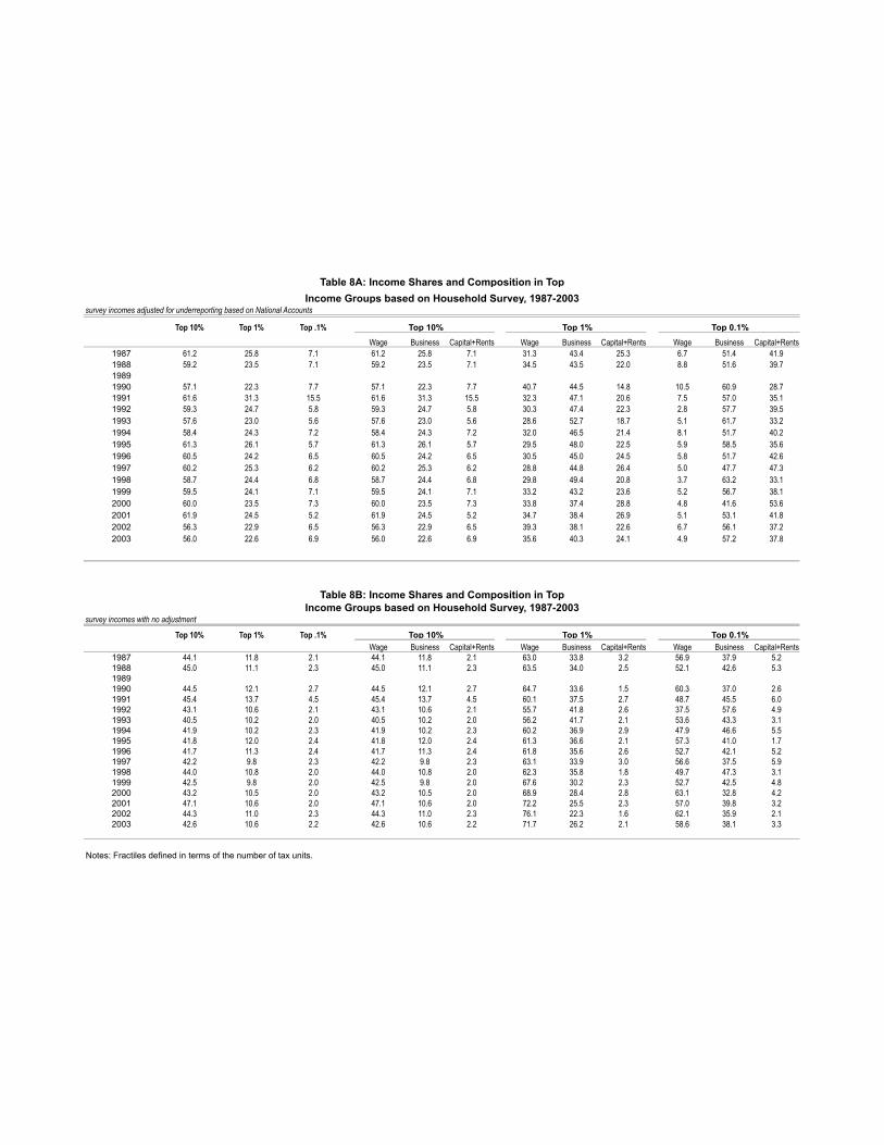
survey incomes adjusted for underreporting based on National Accounts

Top 10% Top 1% Top .1%

Wage Business Capital+Rents Wage Business Capital+Rents Wage Business Capital+Rents1987 61.2 25.8 7.1 61.2 25.8 7.1 31.3 43.4 25.3 6.7 51.4 41.91988 59.2 23.5 7.1 59.2 23.5 7.1 34.5 43.5 22.0 8.8 51.6 39.719891990 57.1 22.3 7.7 57.1 22.3 7.7 40.7 44.5 14.8 10.5 60.9 28.71991 61.6 31.3 15.5 61.6 31.3 15.5 32.3 47.1 20.6 7.5 57.0 35.11992 59.3 24.7 5.8 59.3 24.7 5.8 30.3 47.4 22.3 2.8 57.7 39.51993 57.6 23.0 5.6 57.6 23.0 5.6 28.6 52.7 18.7 5.1 61.7 33.21994 58.4 24.3 7.2 58.4 24.3 7.2 32.0 46.5 21.4 8.1 51.7 40.21995 61.3 26.1 5.7 61.3 26.1 5.7 29.5 48.0 22.5 5.9 58.5 35.61996 60.5 24.2 6.5 60.5 24.2 6.5 30.5 45.0 24.5 5.8 51.7 42.61997 60.2 25.3 6.2 60.2 25.3 6.2 28.8 44.8 26.4 5.0 47.7 47.31998 58.7 24.4 6.8 58.7 24.4 6.8 29.8 49.4 20.8 3.7 63.2 33.11999 59.5 24.1 7.1 59.5 24.1 7.1 33.2 43.2 23.6 5.2 56.7 38.12000 60.0 23.5 7.3 60.0 23.5 7.3 33.8 37.4 28.8 4.8 41.6 53.62001 61.9 24.5 5.2 61.9 24.5 5.2 34.7 38.4 26.9 5.1 53.1 41.82002 56.3 22.9 6.5 56.3 22.9 6.5 39.3 38.1 22.6 6.7 56.1 37.22003 56.0 22.6 6.9 56.0 22.6 6.9 35.6 40.3 24.1 4.9 57.2 37.8

survey incomes with no adjustment

Top 10% Top 1% Top .1%Wage Business Capital+Rents Wage Business Capital+Rents Wage Business Capital+Rents

1987 44.1 11.8 2.1 44.1 11.8 2.1 63.0 33.8 3.2 56.9 37.9 5.21988 45.0 11.1 2.3 45.0 11.1 2.3 63.5 34.0 2.5 52.1 42.6 5.319891990 44.5 12.1 2.7 44.5 12.1 2.7 64.7 33.6 1.5 60.3 37.0 2.61991 45.4 13.7 4.5 45.4 13.7 4.5 60.1 37.5 2.7 48.7 45.5 6.01992 43.1 10.6 2.1 43.1 10.6 2.1 55.7 41.8 2.6 37.5 57.6 4.91993 40.5 10.2 2.0 40.5 10.2 2.0 56.2 41.7 2.1 53.6 43.3 3.11994 41.9 10.2 2.3 41.9 10.2 2.3 60.2 36.9 2.9 47.9 46.6 5.51995 41.8 12.0 2.4 41.8 12.0 2.4 61.3 36.6 2.1 57.3 41.0 1.71996 41.7 11.3 2.4 41.7 11.3 2.4 61.8 35.6 2.6 52.7 42.1 5.21997 42.2 9.8 2.3 42.2 9.8 2.3 63.1 33.9 3.0 56.6 37.5 5.91998 44.0 10.8 2.0 44.0 10.8 2.0 62.3 35.8 1.8 49.7 47.3 3.11999 42.5 9.8 2.0 42.5 9.8 2.0 67.6 30.2 2.3 52.7 42.5 4.82000 43.2 10.5 2.0 43.2 10.5 2.0 68.9 28.4 2.8 63.1 32.8 4.22001 47.1 10.6 2.0 47.1 10.6 2.0 72.2 25.5 2.3 57.0 39.8 3.22002 44.3 11.0 2.3 44.3 11.0 2.3 76.1 22.3 1.6 62.1 35.9 2.12003 42.6 10.6 2.2 42.6 10.6 2.2 71.7 26.2 2.1 58.6 38.1 3.3

Notes: Fractiles defined in terms of the number of tax units.

Top 10% Top 1% Top 0.1%

Table 8A: Income Shares and Composition in TopIncome Groups based on Household Survey, 1987-2003

Top 10% Top 1% Top 0.1%

Table 8B: Income Shares and Composition in TopIncome Groups based on Household Survey, 1987-2003

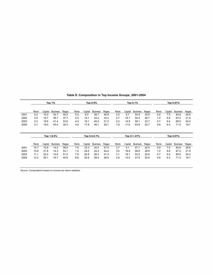
Rents Capital Business Wages Rents Capital Business Wages Rents Capital Business Wages Rents Capital Business Wages2001 6.2 10.0 34.7 49.2 5.0 8.5 39.7 46.8 2.5 6.7 54.9 35.9 0.9 7.5 64.8 26.82002 5.9 19.7 36.7 37.7 4.5 19.1 43.2 33.3 2.7 16.1 54.4 26.7 1.0 9.9 67.2 21.92003 5.3 19.6 41.4 33.6 4.5 19.1 45.2 31.2 2.2 14.9 59.1 23.7 0.7 9.4 69.5 20.42004 5.7 19.0 45.0 30.3 4.9 17.8 48.1 29.1 1.9 11.6 63.8 22.7 0.8 9.3 71.2 18.7

Rents Capital Business Wages Rents Capital Business Wages Rents Capital Business Wages Rents Capital Business Wages

2001 10.7 15.9 14.5 58.9 7.6 10.3 24.2 57.9 3.7 6.1 47.7 42.5 0.9 7.5 64.8 26.82002 10.8 21.8 14.3 53.1 7.4 24.0 24.3 44.4 3.5 18.9 48.8 28.8 1.0 9.9 67.2 21.92003 11.1 23.2 14.6 51.0 7.6 24.8 26.3 41.3 3.1 18.1 53.2 25.6 0.7 9.4 69.5 20.42004 13.2 29.1 16.7 40.9 8.8 25.8 28.5 36.9 2.8 13.5 57.8 25.9 0.8 9.3 71.2 18.7

Source: Computations based on income tax return statistics

Table 9: Composition in Top Income Groups, 2001-2004

Top 1-0.5% Top 0.5-0.1% Top 0.1-.01% Top 0.01%

Top 1% Top 0.5% Top 0.1% Top 0.01%