The Residue Index Theorem of Connes and Moscovici - 2000 - The... · Clay Mathematics Proceedings...
56
Clay Mathematics Proceedings The Residue Index Theorem of Connes and Moscovici Nigel Higson Contents 1. Introduction 1 2. The Cyclic Chern Character 3 3. The Hochschild Character 15 4. Differential Operators and Zeta Functions 21 5. The Residue Cocycle 32 6. The Local Index Formula 36 7. The Local Index Theorem in Cyclic Cohomology 39 Appendix A. Comparison with the JLO Cocycle 47 Appendix B. Complex Powers in a Differential Algebra 51 Appendix C. Proof of the Hochschild Character Theorem 55 References 55 1. Introduction Several years ago Alain Connes and Henri Moscovici discovered a quite general “local” index formula in noncommutative geometry [12] which, when applied to Dirac-type operators on compact manifolds, amounts to an interesting combination of two quite different approaches to index theory. Atiyah and Bott noted that the index of an elliptic operator D may be expressed as a complex residue Index(D) = Res s=0 ( Γ(s) Trace(ε(I + Δ) -s ) ) , where Δ = D 2 (see [1]). Rather surprisingly, the residue may be computed, at least in principle, as the integral of an explicit expression involving the coefficients of D, the metric g, and the derivatives of these functions. However the formulas can be very complicated. In a different direction, Atiyah and Singer developed the crucial link between index theory and K-theory. They showed, for example, that an elliptic operator D on M determines a class [D] ∈ K 0 (M ) c 2004 American Mathematical Society 1
Transcript of The Residue Index Theorem of Connes and Moscovici - 2000 - The... · Clay Mathematics Proceedings...

Clay Mathematics Proceedings
The Residue Index Theorem of Connes and Moscovici
Nigel Higson
Contents
1. Introduction 12. The Cyclic Chern Character 33. The Hochschild Character 154. Differential Operators and Zeta Functions 215. The Residue Cocycle 326. The Local Index Formula 367. The Local Index Theorem in Cyclic Cohomology 39Appendix A. Comparison with the JLO Cocycle 47Appendix B. Complex Powers in a Differential Algebra 51Appendix C. Proof of the Hochschild Character Theorem 55References 55
1. Introduction
Several years ago Alain Connes and Henri Moscovici discovered a quite general“local” index formula in noncommutative geometry [12] which, when applied toDirac-type operators on compact manifolds, amounts to an interesting combinationof two quite different approaches to index theory.
Atiyah and Bott noted that the index of an elliptic operatorD may be expressedas a complex residue
Index(D) = Ress=0
(Γ(s) Trace(ε(I + ∆)−s)
),
where ∆ = D2 (see [1]). Rather surprisingly, the residue may be computed, at leastin principle, as the integral of an explicit expression involving the coefficients of D,the metric g, and the derivatives of these functions. However the formulas can bevery complicated.
In a different direction, Atiyah and Singer developed the crucial link betweenindex theory and K-theory. They showed, for example, that an elliptic operator Don M determines a class
[D] ∈ K0(M)
c©2004 American Mathematical Society
1

2 NIGEL HIGSON
in theK-homology ofM (see [2] for one account of this). As it turned out, this was amajor advance: when combined with the Bott periodicity theorem, the constructionof [D] leads quite directly to a proof of the index theorem.
When specialized to the case of elliptic operators on manifolds, the index for-mula of Connes and Moscovici associates to an elliptic operator D on M a cocyclefor the group HCP ∗(C∞(M)), the periodic cyclic cohomology of the algebra ofsmooth functions on M . In this respect the Connes-Moscovici formula calls tomind the construction of Atiyah and Singer, since cyclic cohomology is related toK-homology by a Chern character isomorphism. But the actual formula for theConnes-Moscovici cocycle involves only residues of zeta-type functions associatedto D. In this respect it calls to mind the Atiyah-Bott formula.
The proper context for the Connes-Moscovici index formula is the noncom-mutative geometry of Connes [7], and in particular the theory of spectral triples.Connes and Moscovici have developed at length a particular case of the index for-mula which is relevant to the transverse geometry of foliations [12, 13]. This work,which involves elaborate use of Hopf algebras, has attracted considerable attention(see the survey articles [8] and [26] for overviews). At the same time, other in-stances of the index formula are beginning to be developed (see for example [9],which among other things gives a good account of the meaning of the term “local”in noncommutative geometry).
The original proof of the Connes-Moscovici formula, which is somewhat in-volved, reduces the local index formula to prior work on the transgression of theChern character, and is therefore is actually spread over several papers [12, 11, 10].Roughly speaking, the residues of zeta functions which appear in the formula arerelated by the Mellin transform to invariants attached to the heat semigroup e−t∆.The heat semigroup figures prominently in the theory of the JLO cocycle in cyclictheory, and so previous work on this subject can now be brought to bear on thelocal index formula.
The main purpose of these notes is to present, in a self-contained way, a newand perhaps more accessible proof of the local index formula. But for the benefit ofthose who are just becoming acquainted with Connes’ noncommutative geometry,we have also tried to provide some context for the formula by reviewing at thebeginning of the notes some antecedent ideas in cyclic and Hochschild cohomology.
As for the proof of the theorem itself, in contrast to the orginal proof of Connesand Moscovici, we shall work directly with the complex powers ∆−z. Our strategyis to find an elementary quantity 〈a0, [D, a1], . . . , [D, ap]〉z (see Definition 4.12), asort of multiple zeta function, which is meromorphic in the argument z, and whoseresidue at z = −p
2 is the complicated combination of residues which appears in theConnes-Moscovici cocycle. The proof of the index formula can then be organized ina fairly conceptual way using the new quantities. The main steps are summarizedin Theorems 5.5, 5.6, 7.1 and 7.12.
The “elementary quantity” 〈a0, [D, a1], . . . , [D, ap]〉z was obtained by emulatingsome computations of Quillen [23] on the structure of Chern character cocycles incyclic theory. Quillen constructed a natural “connection form” Θ in a differentialgraded cochain algebra, along with a “curvature form” K = dΘ+Θ2, for which thequantities
Γ(z)Trace(K−z) =
Γ(z)2πi
Trace(∫
λ−z(λ−K)−1 dλ
)

THE RESIDUE INDEX THEOREM OF CONNES AND MOSCOVICI 3
have components 〈1, [D, a1], . . . , [D, ap]〉z. Taking residues at z = −p2 we get (at
least formally)
Trace(K
p2)
= Resz=− p2〈1, [D, a1], . . . , [D, ap]〉z
Now, in the context of vector bundles with curvature form K, the pth componentof the Chern character is a constant times Trace(K
p2 ). As a result, it is natural to
guess that our elementary quantities 〈· · · 〉z are related to the Chern character andindex theory, after taking residues. All this will be explained in a little more detailat the end of the notes, in Appendix B. Appendix A explains the relation betweenthe Connes-Moscovici cocycle and the JLO cocycle, which was one of the orginalobjects of Quillen’s study and which, as we noted above, played an important inthe original approach to the index formula.
A final appendix presents a proof of Connes’ Hochschild class formula. Thisis essentially a back-formation from the proof of the local index formula presentedhere. (Connes’ Hochschild formula is introduced in Section 3 as motivation for thedevelopment of the local index formula.)
Obviously the whole of the present work is strongly influenced by the work ofConnes and Moscovici. Moreover in several places the computations which followare very similar ones they have carried out in their own work. I am very grateful toboth of them for their encouragement and support. I also thank members of PennState’s Geometric Functional Analysis Seminar, especially Raphael Ponge, for theiradvice, and for patiently listening to early versions of this work.
2. The Cyclic Chern Character
In this section we shall establish some notation and terminology related toFredholm index theory and cyclic cohomology. For obvious reasons we shall fol-low Connes’ approach to cyclic cohomology, which is described for example in hisbook [7, Chapter 3]. Along the way we shall make explicit choices of normalizationconstants.
2.1. Fredholm Index Problems. A linear operator T : V → W from onevector space to another is Fredholm its kernel and cokernel are finite-dimensional,in which case the index of T is defined to be
Index(T ) = dim ker(T )− dim coker(T ).
The index of a Fredholm operator has some important stability properties, whichmake it feasible in many circumstances to attempt a computation of the index evenif computations of the kernel and cokernel, or even their dimensions, are beyondreach.
First, if F : V → W is any finite-rank operator then T + F is also Fredholm,and moreover Index(T ) = Index(T + F ). Second, if V and W are Hilbert spacesthen the set of all bounded Fredholm operators from V to W is an open subsetof the set of all bounded operators in the operator norm-topology, and moreoverthe index function is locally constant. In addition, if K : V → W is any compactoperator between Hilbert spaces (which is to say that K is a norm-limit of finite-rank operators), then T +K is Fredholm, and moreover Index(T ) = Index(T +K).In fact, an important theorem of Atkinson asserts that a bounded linear operatorbetween Hilbert spaces is Fredholm if and only if it is invertible modulo compactoperators. See for example [15].

4 NIGEL HIGSON
The following situation occurs frequently in geometric problems which makecontact with Fredholm index theory. One is presented with an associative algebra Aof bounded operators on a Hilbert space H, and one is given a bounded self-adjointoperator F : H → H with the property that F 2 = 1, and for which, for every a ∈ A,the operator [F, a] = Fa−aF is compact. This setup (or a small modification of it)was first studied by Atiyah [2], who made the following observation related to indextheory and K-theory. Since F 2 = 1 the operator P = 1
2 (P +1) is a projection on H(it is the orthogonal projection onto the +1 eigenspace of F ). If u is any invertibleelement of A then the operator PuP : PH → PH is Fredholm. This is becausethe operator Pu−1P : PH → PH is an inverse, modulo compact operators, and soAtkinson’s theorem, cited above, applies.
A bit more generally, if U = [uij ] is an n × n invertible matrix over A thenthe matrix PUP = [PuijP ], regarded as an operator on the direct sum of n copiesof PH, is a Fredholm operator (for basically the same reason). Now the invertiblematrices over A constitute generators for the (algebraic) K-theory group Kalg
1 (A)(see [22] for details1). It is not hard to see that Atiyah’s index construction givesrise to a homomorphism of groups
IndexF : Kalg1 (A) → Z.
If A is a reasonable2 topological algebra, for instance a Banach algebra, so thattopological K-groups are defined, then the index construction even descends to ahomomorphism
IndexF : Ktop1 (A) → Z.
In short, the data consisting of A and F together provides a supply of Fredholmoperators, and one can investigate in various examples the possibility of determiningthe indices of these Fredholm operators.
2.1. Example. Let A be the algebra of smooth, complex-valued functions onthe unit circle S1, H is the Hilbert space L2(S1), and F is the Hilbert transformon the circle, which maps the trigonometric function exp(2πinx) to exp(2πinx)when n ≥ 0 and to − exp(2πinx) when n < 0. To see that the operators [F, a]are compact, one can first make an explicit computation in the case where a is atrigonometric monomial a(x) = exp(2πinx), with the result that [F, a] is in fact afinite-rank operator. The general case follows by approximating a general a ∈ A bya trigonometric polynomial. In this example one has the famous index formula
Index(PuP ) = − 12πi
∫S1u−1du.
The right hand side is (minus) the winding number of the function u : S1 → C\0.(There is also a simple generalization to matrices U = [uij ].) The topological K1-group here is Z, and the index homomorphism is an isomorphism.
These notes are concerned with formulas for the Fredholm indices which arisefrom certain instances of Atiyah’s construction. We are going to write down a bitmore carefully the basic data for the construction, and then add a first additionalhypothesis to narrow the scope of the problem just a little.
1Except to provide some background context, we shall not use K-theory in these notes.2See the appendix of [3] for a discussion of some types of reasonable topological algebra.

THE RESIDUE INDEX THEOREM OF CONNES AND MOSCOVICI 5
2.2. Definition. Let A be an associative algebra over C. An odd Fredholmmodule over A is a triple consisting of:
(a) a Hilbert space H,(b) a representation of A as bounded operators on H, and(c) a self-adjoint operator F : H → H such that F 2 = 1 and such that [F, π(a)] is
a compact operator, for every a ∈ A.
An even Fredholm module over A consists of the same data as above, together witha self-adjoint operator ε : H → H such that ε2 = 1, such that ε commutes witheach operator π(a), and such that ε anticommutes with F .
Since ε is self-adjoint and since ε2 = 1, the Hilbert space H decomposes as anorthogonal direct sum H = H0⊕H1 in such a way that ε =
(1 00 −1
). The additional
hypothesis imply that
F =(
0 T ∗
T 0
)and π(a) =
(π0(a) 0
0 π1(a)
).
Even Fredholm modules often arise from geometric problems on even-dimensionalmanifolds — hence the terminology. They are actually closer to Atiyah’s originalconstructions in [2] than are the odd Fredholm modules.
Associated to an even Fredholm module there is the following index construc-tion. If p is an idempotent element of A then the operator
π1(p)Fπ0(p) : π0(p)H0 → π1(p)H1
is Fredholm, since π0(p)Fπ1(p) : π1(p)H1 → π0(p)H0 is an inverse, modulo compactoperators. This construction passes easily to matrices, and we obtain a homomor-phism
IndexF : Kalg0 (A) → Z.
which is the counterpart of the index homomorphism we previously constructed inthe odd case.
2.3. Definition. A Fredholm module over A is finitely summable if there issome d ≥ 0 such that for every integer n ≥ d every product of commutators
[F, π(a0)][F, π(a1)] · · · [F, π(an)]
is a trace-class operator. (See [25] for a discussion of trace class operators.)
2.4. Example. The Fredholm module presented in Example 2.1 is finitelysummable: one can take d = 1.
We are going to determine formulas in multi-linear algebra for the indices ofFredholm operators associated to finitely summable Fredholm modules.
2.2. Cyclic Cocycles.
2.5. Definition. A (p+ 1)-linear functional φ : Ap+1 → C is said to be cyclicif
φ(a0, a1, . . . , ap) = (−1)pφ(ap, a0, . . . , ap−1),
for all a0, . . . , ap in A.

6 NIGEL HIGSON
2.6. Definition. The coboundary of a (p+ 1)-linear functional φ : Ap+1 → Cis the (p+ 2)-linear functional
bφ(a0, . . . , ap+1) =p∑j=0
(−1)jφ(a0, . . . , ajaj+1, . . . , ap+1)
+ (−1)p+1φ(ap+1a0, . . . , ap)
A (p+ 1)-multilinear functional φ is a p-cocycle if bφ = 0.
It is easy to check that the coboundary of any coboundary is zero, or in otherwords b2 = 0. Thus every coboundary is a cocycle and as a result we can formwhat are called the Hochschild cohomology groups of A: the pth Hochschild groupis the quotient of the p-cocycles by the p-cocycles which are coboundaries. We willreturn to these groups in Section 3, but for the purposes of index theory we aremuch more interested in the special properties of cyclic cocycles.
2.7. Theorem (Connes). Let φ be a (p+ 1)-linear functional on which is bothcyclic and a cocycle.(a) If p is odd, and if u is an invertible element of A then the quantity
〈φ, u〉 = constant · φ(u−1, u, . . . , u−1, u)
depends only on the class of u in the abelianization of GL1(A), and defines ahomomorphism from the abelianization into C.
(b) If p is even and if e is an idempotent element of A then the quantity
〈φ, e〉 = constant · φ(e, e, . . . , e)
depends only on the equivalence class3 of e. If e1 and e2 are orthogonal, in thesense that e1e2 = e2e1 = 0, then
〈φ, e1 + e2〉 = 〈φ, e1〉+ 〈φ, e2〉.
2.8. Remark. We have inserted as yet unspecified constants into the formu-las for the pairings 〈 , 〉. As we shall see, they are needed to make the pairingsfor varying p consistent with one another, The constants will be made explicit inTheorem 2.27.
2.9. Example. The simplest non-trivial instances of the theorem occur whenp = 1 or p = 2. For p = 1 the explicit conditions on φ are
φ(a0, a1) = −φ(a1, a0)
φ(a0a1, a2)− φ(a0, a1a2) + φ(a2a0, a1) = 0,
while for p = 2 the conditions areφ(a0, a1, a2) = φ(a2, a0, a1)
φ(a0a1, a2, a3)− φ(a0, a1a2, a3) + φ(a0, a1, a2a3)− φ(a3a0, a1, a2) = 0.
The reader who has not done so before ought to try to tackle the theorem for hisor herself in these cases before consulting Connes’ paper [4].
3Two idempotents e and f are equivalent if there are elements x and y of A such that e = xyand f = yx. If A is for example a matrix algebra then two idempotent matrices are equivalent if
and only if their ranges have the same dimension.

THE RESIDUE INDEX THEOREM OF CONNES AND MOSCOVICI 7
The pairings 〈 , 〉 defined by the theorem extend easily to invertible and idem-potent matrices, and thereby define homomorphisms
〈φ, 〉 : Kalg1 (A) → C p odd
〈φ, 〉 : Kalg0 (A) → C p even
The question now arises, can the index homomorphisms constructed in the previoussection be recovered as instances of the above homomorphisms, for suitable cycliccocycles φ? This was answered by Connes, as follows:
2.10. Theorem. Let (A,H,F ) be a finitely summable, odd Fredholm moduleand let n = 2k + 1 be an odd integer such that for all a0, . . . , an in A the product[F, a0] · · · [F, an] is a trace-class operator. The formula
φ(a0, . . . , an
)=
12
Trace(F [F, a0][F, a1] . . . [F, an]
)defines a cyclic n-cocycle on A. If u is an invertible element of A then
φ(u, u−1, . . . , u, u−1) = (−1)k+122k+1 Index(PuP : PH → PH),
where P = 12 (F + 1).
2.11. Theorem. Let (A,H,F ) be a finitely summable, even Fredholm module,and let n = 2k be an even integer such that for all a0, . . . , an in A the product[F, a0] · · · [F, an] is a trace-class operator. The formula
φ(a0, . . . , an
)=
12
Trace(εF [F, a0][F, a1] . . . [F, an]
)defines a cyclic n-cocycle on A. If e is an idempotent element of A then
φ(e, e, . . . , e) = (−1)k Index(eFe : eH0 → H1).
The proofs of these results may be found in [4] or [7, IV.1] (but in the nextsection we shall at least verify that the formulas do indeed define cyclic cocycles).
2.3. Cyclic Cohomology. Throughout this section we shall assume that Ais an associative algebra over C with a mutlilicative identity 1. The definitions foralgebras with an identity are a little different and will be considered later.
It is a remarkable fact that if φ is a cyclic multi-linear functional then so is itscoboundary bφ.4 As a result of this we can form the cyclic cohomology groups ofA:
2.12. Definition. The pth cyclic cohomology group of a complex algebra Ais the quotient HCp(A) of the cyclic p-cocycles by the cyclic p-cocycles which arecyclic coboundaries.
But we are interested in a small modification of the cyclic cohomology groups,called the periodic cyclic cohomology groups of A. There are only two such groups— an even one and and odd one. The even periodic group HCP even(A) in somesense combines all the HC2k(A) into one group, while the odd periodic groupHCP odd(A) does the same for the HC2k+1(A). One reason for considering the
4Note that cyclicity for a (p+1)-linear functional φ has to do with invariance under the action
of the cyclic group Cp+1, whereas cyclicity for bφ has to do with invariance under Cp+2, so to a
certain extent b intertwines the actions of two different groups — this is what is so remarkable.

8 NIGEL HIGSON
periodic groups is that Connes’ construction of the cyclic cocycle associated toa Fredholm module produces not one cyclic cocycle, but one for each sufficientlylarge integer n of the correct parity. As we shall see, the periodic cyclic cohomologygroups provide a framework within which these different cocycles can be comparedwith one another.
The definition of HCP even / odd(A) is, at first sight, a little strange, but afterwe look at some examples it will come to seem more natural.
2.13. Definition. Let A be an associative algebra over C with a multiplicativeidentity element 1. If p is a non-negative integer, then denote by Cp(A) space of(p + 1)-multi-linear maps φ from A into C wich have the property that if aj = 1,for some j ≥ 1, then φ(a0, . . . , ap) = 0. Define operators
b : Cp(A) → Cp+1(A) and B : Cp+1(A) → Cp(A),
by the formulas
bφ(a0, . . . , ap+1) =p∑j=0
(−1)jφ(a0, . . . , ajaj+1, . . . , ap+1)
+ (−1)p+1φ(ap+1a0, . . . , ap)
and
Bφ(a0, . . . , ap) =p∑j=0
(−1)pjφ(1, aj , aj+1, . . . , aj−1).
2.14. Remark. The operator b is the same as the coboundary operator that weencountered in the previous section, except that we are now considering a slightlyrestricted class of multi-linear maps on which b is defined (we should not that asimple computations shows b to be well defined as a map from Cp(A) into Cp+1(A)).In what follows, we could in fact work with all multi-linear functionals, rather thanjust those for which φ(a0, . . . , ap) = 0 when aj = 1 for some j ≥ 1 (although thiswould entail a small modification to the formula for the operator B; see [21]). Thesetup we are considering is a bit more standard, and allows for some slightly simplerformulas.
2.15. Lemma. b2 = 0, B2 = 0 and bB +Bb = 0.

THE RESIDUE INDEX THEOREM OF CONNES AND MOSCOVICI 9
As a result of the lemma, we can assemble from the spaces Cp(A) the followingdouble complex, which is continued indefinitely to the left and to the top.
......
......
. . . B // C3(A)
b
OO
B // C2(A)
b
OO
B // C1(A)
b
OO
B // C0(A)
b
OO
. . . B // C2(A)
b
OO
B // C1(A)
b
OO
B // C0(A)
b
OO
. . . B // C1(A)
b
OO
B // C0(A)
b
OO
. . . B // C0(A)
b
OO
2.16. Definition. The periodic cyclic cohomology of A is the cohomology ofthe totalization of this complex.
Thanks to the symmetry inherent in the complex, all even cohomology groupsare the same, as are all the odd groups. As a result, one speaks of the even and oddperiodic cyclic cohomology groups of A. A cocycle for the even group is a sequence
(φ0, φ2, φ4, . . . ),
where φ2k ∈ C2k, φ2k = 0 for all but finitely many k, and
bφ2k +Bφ2k+2 = 0
for all k ≥ 0. Similarly a cocycle for the odd group is a sequence
(φ1, φ3, φ5, . . . ),
where φ2k+1 ∈ C2k+1, φ2k+1 = 0 for all but finitely many k, and
bφ2k+1 +Bφ2k+3 = 0
for all k ≥ 0 (and in addition Bφ1 = 0).
2.17. Definition. We shall refer to cocycles of the above sort as (b, B)-cocycles.This will help us distinguish between these cocycles and the cyclic cocycles whichwe introduced in the last section.
Suppose now that φn is a cyclic n-cocycle, as in the last section, and supposethat φn has the property that φ(a0, . . . , an) = 0 when some aj is equal to 1. Notethat Connes’ cocycles described in Theorems 2.10 and 2.11 have this property. Bydefinition, bφn = 0, and clearly Bφn = 0 too, since the definition of D involves theinsertion of 1 as the first argument of φn. As a result, the sequence
(0, . . . , 0, φn, 0, . . . ),
obtained by placing φn in position n and 0 everywhere else, is a (b, B)-cocycle. Inthis was we shall from now on regard every cyclic cocycle as a (b, B)-cocycle.

10 NIGEL HIGSON
2.18. Remark. It is known that every (b, B)-cocycle is cohomologous to acyclic cocycle of some degree p (see [21]).
Let us now return to the cocycles which Connes constructed from a Fredholmmodule.
2.19. Theorem. Let (A,H,F ) be a finitely summable, odd Fredholm moduleand let n be an odd integer such that for all a0, . . . , an in A the product [F, a0] · · · [F, an]is a trace-class operator. The formula
chFn(a0, . . . , an
)=
Γ(n2 + 1)2 · n!
Trace(F [F, a0][F, a1] . . . [F, an]
)defines a cyclic n-cocycle on A whose periodic cyclic cohomology class is independentof n.
Proof. Define
ψn+1(a0, . . . , an+1) =Γ(n2 + 2)(n+ 2)!
Trace(a0F [F, a1][F, a2] . . . [F, an+1]
).
It is then straightforward to compute that bψn+1 = − chFn+2 while Bψn+1 = chFn .Hence chFn − chFn+2 is a (b, B)-coboundary.
2.20. Remarks. Obviously, the multiplicative factor Γ( n2 +1)
2n! is chosen to guar-antee that the class of chFn in periodic cyclic cohomology is independent of n.Since b2 = 0, the formula bψn+1 = − chFn+2 proves that chFn+2 is a cocycle (i.e.b chFn+2 = 0). In addition, since it is clear from the definition of the operator Bthat the range of B consists entirely of cyclic multi-linear functionals, the formulaBψn+1 = chFn proves that chFn is cyclic.
2.21. Theorem. Let (A,H,F ) be a finitely summable, even Fredholm moduleand let n be an odd integer such that for all a0, . . . , an in A the product [F, a0] · · · [F, an]is a trace-class operator. The formula
chFn(a0, . . . , an
)=
Γ(n2 + 1)2 · n!
Trace(εF [F, a0][F, a1] . . . [F, an]
)defines a cyclic n-cocycle on A whose periodic cyclic cohomology class is independentof n.
Proof. Define
ψn+1(a0, . . . , an+1) =Γ(n2 + 2)(n+ 2)!
Trace(a0F [F, a1][F, a2] . . . [F, an+1]
)and proceed as before.
2.22. Definition. The cocycle chFn defined in Theorem 2.19 or 2.21 is thecyclic Chern character of the odd or even Fredholm module (A,H,F ).
2.4. Comparison with de Rham Theory. Let M be a smooth, closedmanifold and denote by C∞(M) the algebra of smooth, complex-valued functionson M . For p ≥ 0 denote by Ωp the space of p-dimensional de Rham currents (dualto the space Ωp of smooth p-forms).
Each current c ∈ Ωp determines a cochain φc ∈ Cp(A) for the algebra C∞(M)by the formula
φc(f0, . . . , fp) =∫c
f0df1 · · · dfp.

THE RESIDUE INDEX THEOREM OF CONNES AND MOSCOVICI 11
The following is a simple computation:
2.23. Lemma. If c ∈ Ωp is any p-current on M then
bφc = 0 and Bφc = p · φd∗c,
where d∗ : Ωp → Ωp−1 is the operator which is adjoint to the de Rham differential.
The lemma implies that if we assemble the spaces Ωp into a bicomplex, asfollows,
......
......
. . . 4d∗ // Ω3
0
OO
3d∗ // Ω2
0
OO
2d∗ // Ω1
0
OO
d∗ // Ω0
0
OO
. . . 3d∗ // Ω2
0
OO
2d∗ // Ω1
0
OO
d∗ // Ω0
0
OO
. . . 2d∗ // Ω1
0
OO
d∗ // Ω0
0
OO
. . . d∗ // Ω0
0
OO
then the construction c 7→ φc defines a map from this bicomplex to the bicomplexwhich computes periodic cyclic cohomology of A = C∞(M).
A fundamental result of Connes [4, Theorem 46] asserts that this map of com-plexes is an isomorphism on cohomology:
2.24. Theorem. The inclusion c 7→ φc of the above double complex into the(b, B)-bicomplex induces isomorphisms
HCP evencont (C∞(M)) ∼= H0(M)⊕H2(M)⊕ · · ·
andHCP odd
cont(C∞(M)) ∼= H1(M)⊕H3(M)⊕ · · ·
Here HCP ∗cont(C∞(M)) denotes the periodic cyclic cohomology of M , computed
from the bicomplex of continuous multi-linear functionals on C∞(M).
It follows that an even/odd (b, B)-cocycle for C∞(M) is something very like afamily of closed currents on M of even/odd degrees.
Connes’ theorem is proved by first identifying the (continuous) Hochschild co-homology of the algebra A = C∞(M). Lemma 2.23 shows that there is a map ofcomplexes
Ω0 0 //
Ω1
0 // · · · 0 // Ωn
0 // 0
0 // . . .
C0(A)b
// C1(A)b
// · · ·b
// Cn(A)b
// Cn+1(A)b
// . . .

12 NIGEL HIGSON
in which the vertical maps come from the construction c 7→ φc. The following resultis known as the Hochschild Kostant Rosenberg theorem (see [21]), although thisprecise formulation is due to Connes [4].
2.25. Theorem. The above map induces an isomorphism from Ωp to the pthcontinuous Hochschild cohomology group HHp
cont(C∞(M)).
Let us conclude this section with a few brief remarks about non-periodic cycliccohomology groups. We already noted that every cyclic p-cocycle determines a(B, b)-cocycle (even or odd, according to the parity of p). In view of the HochschildKostant Rosenberg theorem, and in view of the fact that every cyclic p-cocycle is inparticular a Hochschild p-cocycle, so that if A is any algebra then there is a naturalmap from pth cyclic cohomology group HCp(A), as given in Definition 2.12, intothe Hochschild group HHp(A), it might be thought that when A = C∞(M) thecyclic p-cocycles correspond to the summand Hp(M) in Theorem 2.24. But this isnot exactly right. It cannot be right because if a (b, B)-cocycle is cohomologousto a cyclic p-cocycle, it may be shown that it is also cohomologous to a cyclic(p+ 2)-cocycle, and to a cyclic (p+ 4)-cocycle, and so on. So when A = C∞(M) asingle cyclic p-cocycle can encode information not just about closed p-currents, butalso about closed (p − 2)-currents, closed (p − 4)-currents, and so on. The preciserelation, again discovered by Connes, is as follows:
2.26. Theorem. Denote by Zp(M) the set of closed de Rham k-currents onM . There are isomorphisms
HC2kcont(C
∞(M)) ∼= H0(M)⊕H2(M)⊕ · · · ⊕H2k−2(M)⊕ Z2k(M)
and
HC2k+1cont (C∞(M)) ∼= H1(M)⊕H3(M)⊕ · · · ⊕H2k−1(M)⊕ Z2k+1(M).
Here HC∗cont(C∞(M)) denotes the cyclic cohomology of M , computed from the
complex of continuous cyclic multi-linear functionals on C∞(M).
2.5. Pairings with K-Theory. The pairings described in Theorem 2.7 be-tween cyclic cocycles and K-theory have the following counterparts in periodiccyclic theory.
2.27. Theorem (Connes). Let A be an algebra with a multiplicative identity.(a) If φ = (φ1, φ3, . . . ) is an odd (b, B)-cocycle for A, and u is an invertible element
of A, then the quantity
〈φ, u〉 =1
Γ( 12 )
∞∑k=0
(−1)k+1k!φ2k+1(u−1, u, . . . , u−1, u)
depends only on the class of u in the abelianization of GL1(A) and the periodiccyclic cohomology class of φ, and defines a homomorphism from the abelianiza-tion into C.
(b) If φ = (φ0, φ2, . . . ) is an even (b, B)-cocycle for A, and e is an idempotentelement of A, then the quantity
〈φ, e〉 = φ0(e) +∞∑k=1
(−1)k(2k)!k!
φ2k(e−12, e, e, . . . , e).

THE RESIDUE INDEX THEOREM OF CONNES AND MOSCOVICI 13
depends only on the equivalence class of e and the periodic cyclic cohomologyclass of φ. Moreover if e1 and e2 are orthogonal idempotents in A, then
〈φ, e1 + e2〉 = 〈φ, e1〉+ 〈φ, e2〉.
Proof. See [16] for the odd case and [17] for the even case.
2.28. Example. Putting together Theorem 2.10 with the formula (a) in The-orem 2.27, we see that if (A,H,F ) is a finitely summable, odd Fredholm module,and if u is an invertible element of A, then
〈chFn , u〉 = Index(PuP : PH → PH),
where P is the idempotent P = 12 (F + 1), and the odd integer n is large enough
that the Chern character is defined. Similarly, if (A,H,F ) is an even Fredholmmodule and if e is an idempotent element of A then
〈chFn , e〉 = Index(eFe : eH0 → eH1),
for all even n which again are large enough that the Chern character is defined.
2.29. Remarks. The pairings described in Theorem 2.27 extend easily to thealgebraic K-theory groups Kalg
1 (A) and Kalg0 (A).
2.6. Improper Cocycles and Coefficients. We are going to describe toextensions of the notion of (b, B)-cocycle which will be useful in these notes.
If V is a complex vector space and p is a non-negative integer, then let usdenote by Cp(A, V ) space of (p + 1)-multi-linear maps φ from A into V for whichφ(a0, . . . , ap) = 0 whenever aj = 1 for some j ≥ 1.
Define operators
b : Cp(A, V ) → Cp+1(A, V ) and B : Cp+1(A, V ) → Cp(A, V ),
by the same formulas we used previously:
bφ(a0, . . . , ap+1) =p∑j=0
(−1)jφ(a0, . . . , ajaj+1, . . . , ap+1)
+ (−1)p+1φ(ap+1a0, . . . , ap)
and
Bφ(a0, . . . , ap) =p∑j=0
(−1)pjφ(1, aj , aj+1, . . . , aj−1).

14 NIGEL HIGSON
Then assemble the double complex
......
......
. . . B // C3(A, V )
b
OO
B // C2(A, V )
b
OO
B // C1(A, V )
b
OO
B // C0(A, V )
b
OO
. . . B // C2(A, V )
b
OO
B // C1(A, V )
b
OO
B // C0(A, V )
b
OO
. . . B // C1(A, V )
b
OO
B // C0(A, V )
b
OO
. . . B // C0(A, V )
b
OO
just as before.
2.30. Definition. The periodic cyclic cohomology of A, with coefficients in Vis the cohomology of the totalization of this complex.
It is easy to check that the periodic cyclic cohomology of A with coefficients inV is just the space of homomorphisms into V from the periodic cyclic cohomologyof A with coefficients in C (the latter is the “usual” periodic cyclic cohomology ofA). Nevertheless the concept of coefficients will be a convenient one for us.
If we totalize the (b, B)-bicomplex (either the above one involving V or theprevious one without V ) by taking a direct product of cochain groups along thediagonals instead of a direct sum, then we obtain a complex with zero cohomology.
2.31. Definition. We shall refer to cocycles for this complex, consisting inthe even case of sequences (φ0, φ2, φ4, . . . ), all of whose terms may be nonzero, asimproper (b, B)-cocycles.
On its own, an improper periodic (b, B)-cocycle has no cohomological signifi-cance, but once again the concept will be a convenient one for us. For example inSection 5 we shall construct a fairly simple improper (b, B)-cocycle with coefficientsin the space V of meromorphic functions on C. By taking residues at 0 ∈ C weshall obtain a linear map from V to C, and applying this linear map to our cocyclewe shall obtain in Section 5 a proper (b, B)-cocycle with coefficients in C.
2.7. Nonunital Algebras. If the algebra A has no multiplicative unit thenwe define periodic cyclic cohomology as follows. Denote by A the algebra obtained

THE RESIDUE INDEX THEOREM OF CONNES AND MOSCOVICI 15
by adjoining a unit to A and form the double complex
......
......
. . . B // C3(A)
b
OO
B // C2(A)
b
OO
B // C1(A)
b
OO
B // C0(A)
b
OO
. . . B // C2(A)
b
OO
B // C1(A)
b
OO
B // C0(A)
b
OO
. . . B // C1(A)
b
OO
B // C0(A)
b
OO
. . . B // C0(A)
b
OO
in which the spaces Cp(A) are, as before, the (p+ 1)-multlinear functionals φ fromA into C with the property that φ(a0, . . . , ap) = 0 whenever aj = 1 for some j ≥ 1,and in which C0(A) is the space of linear functionals on A (not on A). If weinterpret b : C0(A) → C1(A) using the formula
bφ(a0, a1) = φ(a0a1)− φ(a1a0) = φ(a0a1 − a1a0)
then the differential is well defined, since the commutator a0a1−a1a0 always belongsto A, even when a0, a1 ∈ A.
2.32. Definition. The periodic cyclic cohomology of A is the cohomology ofthe totalization of the above complex. A (b, B)-cocycle for A is a cocycle for theabove complex.
2.33. Remark. The periodic cyclic cohomology of a non-unital algebra A isisomorphic to the kernel of the restriction map from HCP ∗(A) to HCP ∗(C).
2.34. Definition. By a cyclic p-cocycle on A we shall mean a cyclic cocycle φon A for which φ(a0, . . . , ap) = 0 whenever aj = 1 for some j.
3. The Hochschild Character
The purpose of this section is to provide some motivation for the developmentof the local index formula in cyclic cohomology by describing an antecedent formulain Hochschild cohomology.
3.1. Spectral Triples. Examples of Fredholm modules arising from geometryoften involve the following structure.
3.1. Definition. A spectral triple is a triple (A,H,D) consisting of:(a) An associative algebra A of bounded operators on a Hilbert space H, and(b) An unbounded self-adjoint operator D on H such that
(i) for every a ∈ A the operators a(D ± i)−1 are compact, and(ii) for every a ∈ A, the operator [D, a] is defined on domD and extends to a
bounded operator on H.

16 NIGEL HIGSON
3.2. Remark. In item (b) we require that D be self-adjoint in the sense ofunbounded operator theory. This means that D is defined on some dense domaindomD ⊆ H, that 〈Du, v〉 = 〈u,D〉, for all u, v ∈ domD, and that the operators(D ± i) map domH bijectively onto H. In item (ii) we require that each a ∈ Amap domD into itself.
3.3. Example. Let A = C∞(S1), let H = L2(S1) and let D = 12πi
ddx . The
operator D, defined initially on the smooth functions in H = L2(S1) (we arethinking now of S1 as R/Z), has a unique extension to a self-adjoint operatoron H, and the triple (A,H,D) incorporating this extension is a spectral triple inthe sense of Definition 3.1.
3.4. Remark. If the algebra A has a unit, which acts as the identity operatoron the Hilbert space H, then item (i) is equivalent to the assertion that (D ± i)−1
be compact operators, which is equivalent to the assertion that there exist anorthonormal basis for H consisting of eigenvectors vj for D, with eigenvalues λjconverging to ∞ in absolute value.
In a way which is similar to our treatment of Fredholm modules, we shall calla spectral triple even if the Hilbert space H is equipped with a self-adjoint gradingoperator ε, decomposing H as a direct sum H = H0 ⊕ H1, such that ε maps thedomain of D into itself, anitcommutes with D, and commutes with every a ∈ A.Spectral triples without a grading operator will be referred to as odd.
Let (A,H,D) be a spectral triple, and assume that D is invertible. In the polardecomposition D = |D|F of D the operator F is self-adjoint and satisifies F 2 = 1.
3.5. Lemma. If (A,H,D) is a spectral triple (A,H,F ) is a Fredholm modulein the sense of Definition 2.2.
3.6. Example. The Fredholm module described in Example 2.1 is obtained inthis way from the spectral triple of Example 3.3, after we make a small modificationto D to make it invertible — for example by replacing 1
2πiddx with 1
2πiddx + 1
2 .
3.2. The Residue Trace. We are going to develop for spectral triples a re-finement of the notion of finite summability that we introduced for Fredholm mod-ules. For this purpose we need to quickly review the following facts about compactoperators and their singular values (see [25] for more details).
3.7. Definition. If K is a compact operator on a Hilbert space then thesingular value sequence µj of K is defined by the formulas
µj = infdim(V )=j−1
supv⊥V
‖Kv‖‖v‖
j = 1, 2, . . . .
The infimum is over all linear subspaces of H of dimension j − 1. Thus µ1 isjust the norm of K, µ2 is the smallest possible norm obtained by restricting K toa codimension 1 subspace, and so on.
The trace ideal is easily described in terms of the sequence of singular values:
3.8. Lemma. A compact operator K belongs to the trace ideal if and only if∑j µj < ∞. Moreover if K is a positive, trace-class operator then Trace(K) =∑j µj.

THE RESIDUE INDEX THEOREM OF CONNES AND MOSCOVICI 17
Now, any self-adjoint trace-class operator can be written as a difference of posi-tive, trace-class operators, K = K(1)−K(2), and we therefore have a correspondingformula for the trace
Trace(K) = Trace(K(1))− Trace(K(2)) =∑j
µ(1)j −
∑j
µ(2)j .
And since every trace-class operator is a linear combination of two self-adjoint,trace-class operators, we can go on to obtain a formula for the trace of a generaltrace-class operator.
We are going to define a new sort of trace by means of formulas like the oneabove.
3.9. Definition. Denote by L1,∞(H) the set of all compact operators K onH for which
N∑j=1
µj = O(logN).
Thus every trace-class operator belongs to L1,∞(H) but operators in L1,∞(H) neednot be trace class, since the sum
∑j µj is permitted to diverge logarithmically.
3.10. Remark. The set L1,∞(H) is a two-sided ideal in B(H).
Suppose now that we are given a linear subspace of L1,∞(H) consisting ofoperators for which the sequence of numbers
1logN
N∑j=1
µj
is not merely bounded but in fact convergent. It may be shown using fairly standardsingular value inequalities that the functional Trω which assigns to each positiveoperator in the subspace the limit of the sequence is additive:
Trω(K(1)) + Trω(K(2)) = Trω(K(1) +K(2)).
As a result, if we assume that the linear subspace we are given is spanned by itspositive elements, the prescription Trω extends by linearity from positive operatorsto all operators and yields a linear functional.
A theorem of Dixmier [14] (see also [7, Section IV.2]) improves this constructionby replacing limits with generalized limits, thereby obviating the need to assumethat the sequence of partial sums 1
logN
∑Nj=1 µj is convergent:
3.11. Theorem. There is a linear functional Trω : L1,∞(H) → C with thefollowing properties:(a) If K ≥ 0 then Trω(K) depends only on the singular value sequence µj, and(b) If K ≥ 0 then lim infN 1
logN
∑Nj=1 µj ≤ Trω(K) ≤ lim supN
1logN
∑Nj=1 µj.
It follows from (a) that Trω(K) = Trω(U∗KU) for every positive K ∈ L1,∞(H)and every unitary operator U on H. Since the positive operators in L1,∞(H) spanL1,∞(H), it follows that Trω(T ) = Trω(U∗TU), for every T ∈ L1,∞(H) and everyunitary operator U . Replacing T by U∗T we get Trω(UT ) = Trω(TU), for everyT ∈ L1,∞(H) and every unitary U . Since the unitary operators span all of B(H),we finally conclude that
Trω(ST ) = Trω(TS),

18 NIGEL HIGSON
for every T ∈ L1,∞(H) and every bounded operator S.
3.12. Remark. The Dixmier trace Traceω is not unique — depends on a choiceof suitable generalized limit for the sequence of partial sums 1
logN
∑Nj=1 µj . But
of course it is unique on (positive) operators for which this sequence is convergent,which turns out to be the case in many geometric examples.
3.3. The Hochschild Character Theorem. If (A,H,F ) is a finitely sum-mable Fredholm module then Connes’ cyclic Chern character chFn is defined forall large enough n of the correct parity (even or odd, according as the Fredholmmodule is even or odd). It is a cyclic n-cocycle, and in particular, disregarding itscyclicity, it is a Hochschild n-cocycle. We are going to present a formula for theHochschild cohomology class of this cocycle, in certain cases.
3.13. Lemma. Let (A,H,D) be a spectral triple, and let n be a positive integer.Assume that D is invertible and that
a · |D|−n ∈ L1,∞(H),
for every a ∈ A. Then the associated Fredholm module (A,H,F ) has the propertythat the operators
[F, a0][F, a1] · · · [F, an]are trace-class, for every a0, . . . , an ∈ A. In particular, the Fredholm module(A,H,F ) is finitely summable and if n has the correct parity, then the Chern char-acter chFn is defined.
3.14. Definition. A spectral triple (A,H,D) is regular if there exists an al-gebra B of bounded operators on H such that(a) A ⊆ B and [D,A] ⊆ B, and(b) if b ∈ B then b maps the domain of |D| (which is equal to the domain of D)
into itself, and moreover |D|B −B|D| ∈ B.
3.15. Example. The spectral triple (C∞(S1), L2(S1), D) of Example 3.3 isregular.
3.16. Remark. We shall look at the notion of regularity in more detail inSection 4, when we discuss elliptic estimates.
We can now state Connes’ Hochschild class formula:
3.17. Theorem. Let (A,H,D) be a regular spectral triple. Assume that D isinvertible and that for some positive integer n of the same parity as the triple, andevery a ∈ A,
a · |D|−n ∈ L1,∞(H).
The Chern character chFn of Definition 2.22 is cohomologous, as a Hochschild co-cycle, to the cocycle
Φ(a0, . . . , an) =Γ(n2 + 1)n · n!
Traceω(εa0[D, a1][D, a2] · · · [D, an]|D|−n).
Here ε is 1 in the odd case, and the grading operator on H in the even case.
3.18. Remark. Actually this is a slight strengthening of what is actually prov-able. For the correct statement, see Appendix C.

THE RESIDUE INDEX THEOREM OF CONNES AND MOSCOVICI 19
3.4. A Simple Example. We shall prove Theorem 3.17 in Appendix C, as aby-product of our proof of the local index theorem (at the moment, it is probablynot even obvious that the functional Φ given in the theorem is a Hochschild cocycle).Right now what we want to do is to compute a simple example of the Hochschildcocycle Φ.
We shall consider the spectral triple (C∞(S1), L2(S1), D), where D is theunique self-adjoint extension of the operator 1
2πiddx + 1
2 (recall that the term 12
was added to guarantee that D is invertible).The operator D is diagonalizable, with eigenfunctions en(x) = exp(2πinx) and
eigenvalues n+ 12 , where n ∈ Z. We see then that |D| given by the formula
|D|en = |n+ 12 |en (n ∈ Z).
As a result, |D|−1 ∈ L1,∞(H), and a brief computation shows that
Traceω(|D|−1) = 2.
3.19. Lemma. If f ∈ C(S1) then Traceω(f · |D|−1) = 2∫S1 f(x) dx.
Proof. The linear functional f 7→ Traceω f · |D|−1 is positive, and so by theRiesz representation theorem it is given by integration against a Borel measureon S1. But the functional, and hence the measure, is rotation invariant. Thisproves that the measure is a multiple of Lebesgue measure, and the computationTrω(|D|−1) = 2 fixes the multiple.
With this computation in hand, we can now determine the cocycle Φ whichappears in Theorem 3.17:
Φ(f0, f1) = Traceω(f0[D, f1]|D|−1) =1πi
∫S1f0(x)f ′1(x) dx.
Now if a0, a1 ∈ C∞(S1), and if Ψ is any 1-cocycle which is in fact a Hochschildcoboundary, then it is easily computed that Ψ(a0, a1) = 0. As a result, of Theo-rem 3.17 it therefore follows that
Γ( 32 ) · 1
2 Trace(F [F, a0][F, a1])def= chF1 (a0, a1) = Γ( 3
2 )Φ(a0, a1)
If we combine this with the Fredholm index formula in Theorem 2.10 we arrive ata proof of the well-known index formula
Index(PuP ) = − 14 Trace(F [F, u−1][F, u]) = − 1
2Φ(u−1, u) = − 12πi
∫S1u−1du
associated to an invertible element u ∈ C∞(S1), which we already mentioned inExample 2.1.
3.20. Remark. In this very simple example we have determined not only theHochschild cocycle Φ but also the cyclic cocycle chF1 . This is an artifact of the low-dimensionality of the example: the natural map from the first cyclic cohomologygroup into the first Hochschild group happens always to be injective. In higherdimensional examples a determination of Φ will in general stop quite a bit short ofa determination of chFn .
20 NIGEL HIGSON
3.5. Weyl’s Theorem. The simple computation which we carried out abovehas a general counterpart which originates with a famous theorem of Weyl. Weshall state the theorem in the context of Dirac-type operators, for which we referthe reader to Roe’s introductory text [24] (this book also contains a proof of Weyl’stheorem).
3.21. Theorem. Let M be a closed Riemannian manifold of dimension n,and let D be a Dirac-type operator on M , acting on the sections of some complexHermitian vector bundle S over M . The operator D has a unique self-adjointextension, and |D|−n ∈ L1,∞(H). Moreover
Traceω(|D|−n) =dim(S)(2√π)n
Vol(M)Γ(n2 + 1)
.
3.22. Remark. If D is not invertible then we define |D|−n by for example|D|−1 = |D + P |−n, where P is the orthogonal projection onto the kernel of D.(Incidentally, we might note that altering an operator in L1,∞(H) by any finiterank operator — or indeed any trace-class operator — has no effect on the Dixmiertrace.)
The theorem may be extended, as follows:
3.23. Theorem. Let M be a closed Riemannian manifold of dimension n,and let D be a Dirac-type operator on M , acting on the sections of some complexHermitian vector bundle S over M . The operator D has a unique self-adjointextension, and |D|−n ∈ L1,∞(H). If F is any endomorphism of S then
Traceω(|D|−n) =1
(2√π)nΓ(n2 + 1)
∫M
trace(F (x)) dx.
Thanks to the theorem, the Hochschild character Φ of Theorem 3.17 may becomputed in the case where A = C∞(M), H = L2(S), and D is a Dirac-typeoperator acting on sections of S (it may be shown that this consitutes an exam-ple of a regular spectral triple; compare Section 4). The commutators [D, a] areendomorphisms of S, and so
Φ(a0, . . . , an) =1
(2√π)nΓ(n2 + 1)
∫M
trace(εa0[D, a1] · · · [D, an]) dx.
3.24. Remark. In many cases the pointwise trace which appears here can befurther computed. For example if D is the Dirac operator associated to a Spinc-structure on M then we obtain the simple formula
Φ(a0, . . . , an) =1
(2√π)nΓ(n2 + 1)
∫M
a0da1 · · · dan.
In summary, we see that Φ(a0, . . . , an) is an integral over M of an explicit ex-pression involving the aj and their derivatives. Unfortunately, in higher dimensions,this very precise information about Φ is not enough to deduce an index theorem,since it is impossible to recover the pairing between cyclic coycles and idempotentsor invertibles from the Hochschild cohomology class of the cyclic cocycle. For thepurposes of index theory we need to obtain a similar formula for the cyclic cocyclechFn itself, or for a cocycle which is cohomologous to it in cyclic or periodic theory.This is what the Connes-Moscovici formula achieves.
THE RESIDUE INDEX THEOREM OF CONNES AND MOSCOVICI 21
The formula involves in a crucial way a residue trace which in certain circum-stances extends to a certain class of operators, including some unbounded operators,2 times the Dixmier trace on L1,∞(H). We shall discuss this in detail in the nextsection, but we shall conclude here with a somewhat vague formulation of the localindex formula, to give the reader some idea of the direction in which we are heading.The statement will be refined in the coming sections.
3.25. Theorem. Let (A,H,D) be a suitable even spectral triple5 and let (A,H,F )be the associated Fredholm module. The Chern character chFn is cohomologous, asa (b, B)-cocycle to the cocycle φ = (φ0, φ2, . . . ) given by the formulas
φp(a0, . . . , ap) =∑k≥0
cpk Res Tr(εa0[D, a1](k1) · · · [D, ap](kp)∆− p
2−|k|).
The sum is over all multi-indices (k1, . . . , kp) with non-negative integer entries, andthe constants cpk are given by the formula
cpk =(−1)k
k!Γ(k1 + · · ·+ kp + p
2 )(k1 + 1)(k1 + k2 + 2) · · · (k1 + · · ·+ kp + p)
.
The operators X(k) are defined inductively by X(0) = X and X(k) = [D2, X(k−1)].
3.26. Remark. Note that when p = n and k = 0 we obtain the term
Γ(n2 )n!
Res Tr(εa0[D, a1] · · · [D, ap]|D|−n
)=
2Γ(n2 )n!
Traceω(εa0[D, a1] · · · [D, ap]|D|−n
)=
Γ(n2 + 1)n · n!
Traceω(εa0[D, a1] · · · [D, ap]|D|−n
).
Thus we recover precisely the Hochschild cocycle of Theorem 3.17. The relationbetween Theorem 3.17 and the local index formula will be further discussed inAppendix C.
4. Differential Operators and Zeta Functions
Apart from cyclic theory, the local index theorem requires a certain amount ofHilbert space operator theory. We shall develop the necessary topics in this section,beginning with a very rapid review of the basic theory of linear elliptic operatorson manifolds.
4.1. Elliptic Operators on Manifolds. Let M be a smooth, closed man-ifold, let S be a smooth vector bundle over M . Let us equip M with a smoothmeasure and S with an inner product, so that we can form the Hilbert spaceL2(M,S).
Let D be the algebra of linear differential operators on M acting on smoothsections of S. This is an associative algebra of operators and it is filtered by theusual notion of order of a differential operator: an operator X has order q or less ifany local coordinate system it can be written in the form
X =∑|α|≤q
aα(x)∂α
∂xα,
5There is an analogous theorem in the odd case.

22 NIGEL HIGSON
where α is a multi-index (α1, . . . , αn) and |α| = α1 + · · ·+ αn.If s is a non-negative integer then the space of order s or less operators is a
finitely generated module over the ring C∞(M). If X1, . . . , XN is a generating setthen the Sobolev space W s(M,S) is defined to be the completion of C∞(M,S)induced from the norm
‖φ‖2W s(M,S) =∑j
‖Xjφ‖2L2(M,S).
Different choices of generating set result in equivalent norms and the same spaceW s(M,S). Every differential operator of order q extends to a bounded linearoperator from W s(M,S) to W s−q(M,S), for all s ≥ q. The Sobolev EmbeddingTheorem implies that that ∩s≥0W
s(M,S) = C∞(M,S).Now let ∆ be a linear elliptic operator of order r. The reader unfamiliar with
the definition of ellipticity can take the following basic estimate as the definition:if ∆ is elliptic of order r, then there is some ε > 0 such that
‖∆φ‖W s(M,S) + ‖φ‖L2(M,S) ≥ ε‖φ‖W s+r(M,S),
for every φ ∈ C∞(M,S).Suppose now that ∆ is also positive, which is to say that 〈∆φ, φ〉L2(M,S) ≥ 0,
for all φ ∈ C∞(M,S). It may be shown then that ∆ is essentially self-adjoint onthe domain C∞(M,S), and for s ≥ 0 we can define the linear spaces
Hs = dom(∆sr ) ⊆ H,
which are Hilbert spaces in the norm
‖φ‖2Hs = ‖φ‖2L2 + ‖∆ rs ‖2L2 .
It follows from the basic estimate that Hs = W s(M,S).Let us say that an operator ∆ of order r operator is of scalar type if in every
local coordinate system ∆ can be written in the form
∆ =∑|α|≤r
aα(x)∂α
∂xα,
where the aα(x), for |α| = r, are scalar multiples of the identity operator (acting onthe fiber Sx of S). Good examples are the Laplace operators ∆ = ∇∗∇ associatedto affine connections on S, which are positive, elliptic of order 2, and of scalar type.Other examples are the squares of Dirac-type operators on Riemannian manifolds.If ∆ is of scalar type then
order([∆, X]) ≤ order(X) + order(∆)− 1
(whereas the individual products X∆ and ∆X have one greater order, in general).The following theorem, which is quite well known, will be fundamental to what
follows in these notes. For a proof which is somewhat in the spirit of these notessee [19].
4.1. Theorem. Let ∆ be elliptic of order r, positive and of scalar type, andassume for simplicity that ∆ is invertible as a Hilbert space operator. Let X be anydifferential operator. If Re(z) is sufficiently large then the operator X∆−z is oftrace class. Moreover the function ζ(z) = Trace(X∆−z) extends to a meromorphicfunction on C with only simple poles.

THE RESIDUE INDEX THEOREM OF CONNES AND MOSCOVICI 23
4.2. Remarks. The assumption that ∆ is of scalar type is not necessary, butit simpifies the proof. and covers the cases of interest. The meaning of the complexpower ∆−z will be clarified in the coming paragraphs.
4.2. Abstract Differential Operators. In this section we shall give abstractcounterparts of the ideas presented in the previous section.
Let H be a complex Hilbert space. We shall assume as given an unbounded,positive, self-adjoint operator ∆ on H. The operator ∆ and its powers ∆k areprovided with definite domains dom(∆k) ⊆ H, which are dense subspaces of H.We shall denote by H∞ the intersections of the domains of all the ∆k:
H∞ = ∩∞k=1 dom(∆k).
We shall assume as given an algebra D(∆) of linear operators on the vector spaceH∞. We shall assume the following things about D(∆):6
(i) IfX ∈ D(∆) then [∆, X] ∈ D(∆) (we shall not insist that ∆ belongs to D(∆)).(ii) The algebra D(∆) is filtered,
D(∆) = ∪∞q=0Dq(∆) (an increasing union).
We shall write order(X) ≤ q to denote the relation X ∈ Dq(∆). Sometimeswe shall use the term “differential order” to refer to this filtration. This issupposed to call to mind the standard example, in which order(X) is the orderof X as a differential operator.
(iii) There is an integer r > 0 (the “order of ∆”) such that
order([∆, X]) ≤ order(X) + r − 1
for every X ∈ D(∆).To state the final assumption, we need to introduce the linear spaces
Hs = dom(∆sr ) ⊆ H
for s ≥ 0. These are Hilbert spaces in their own right, in the norms
‖v‖2s = ‖v‖2 + ‖∆ sr v‖2.
The following key condition connects the algebraic hypotheses we have placed onD(∆) to operator theory:
(iv) If X ∈ D(∆) and if order(X) ≤ q then there is a constant ε > 0 such that
‖v‖q + ‖v‖ ≥ ε‖Xv‖, ∀v ∈ H∞.
4.3. Example. The standard example is of course that in which ∆ is a Laplace-type operator ∆ = ∇∗∇, or ∆ is the square of a Dirac-type operator, on a closedmanifoldM and D(∆) is the algebra of differential operators onM . We can obtain aslightly more complicated example by dropping the assumption that M is compact,and defining D(∆) to be the algebra of compactly supported differential operatorson M (∆ is still a Lapacian or the square of a Dirac operator). Item (i) above wasformulated with the non-compact case in mind.
4.4. Remark. In the standard example the “order” r of ∆ is r = 2. But otherorders are possible. For example Connes and Moscovici consider an importantexample in which r = 4.
6Various minor modifications of these axioms are certainly possible.

24 NIGEL HIGSON
4.5. Remark. For the purposes of these notes we could get by with somethinga little weaker than condition (iv), namely this:
(iv′) If X ∈ D(∆) and if order(X) ≤ kr then there is a constant ε > 0 suchthat
‖∆kv‖+ ‖v‖ ≥ ε‖Xv‖, ∀v ∈ H∞.
The advantage of this condition is that it involves only integral powers of theoperator ∆ (in contrast the ‖ ‖s involve fractional powers of ∆). Condition (iv′) istherefore in principle easier to verify. However in the main examples, for instancethe one developed by Connes and Moscovici in [12], the stronger condition holds.
4.6. Definition. We shall refer to an algebra D(∆) (together with the distin-guished operator ∆) satisfying the axioms (i)-(iv) above as an algebra of generalizeddifferential operators.
4.7. Lemma. If X ∈ D(∆), and if X has order q or less, then for every s ≥ 0the operator X extends to a bounded linear operator from Hs+q to Hs.
Proof. If s is an integer multiple of the order r of ∆ then the lemma followsimmediately from the elliptic estimate above. The general case (which we shall notactually need) follows by interpolation.
4.3. Zeta Functions. Let D(∆) be an algebra of generalized differential oper-ators, as in the previous sections. We are going to define certain zeta-type functionsassociated with D(∆).
To simplify matters we shall now assume that the operator ∆ is invertible. Thisassumption will remain in force until Section 6, where we shall first consider moregeneral operators ∆.
The complex powers ∆−z may be defined using the functional calculus. Theyare, among other things, well-defined operators on the vector space H∞.
4.8. Definition. The algebra D(∆) has finite analytic dimension if there issome d ≥ 0 with the property that if X ∈ D(∆) has order q or less, then, for everyz ∈ C with real part greater than q+d
r , the operator X∆−z extends by continuity toa trace-class operator on H (here r is the order of ∆, as described in Section 4.2).
4.9. Remark. The condition on Re(z) is meant to imply that the order ofX∆−z is less than −d. (We have not yet assigned a notion of order to operatorssuch as X∆−z, but we shall do so in Definition 4.15.)
4.10. Definition. The smallest value d ≥ 0 with the property described inDefinition 4.8 will be called the analytic dimension of the algebra D(∆).
Assume that D(∆) has finite analytic dimension d. If X ∈ D(∆) and iforder(X) ≤ q then the complex function Trace(X∆−z) is holomorphic in the righthalf-plane Re(z) > q+d
r .
4.11. Definition. An algebra D(∆) of generalized differential operators whichhas finite analytic dimension has the analytic continuation property if for everyX ∈ D(∆) the analytic function Trace(X∆−z), defined initially on a half-plane inC, extends to a meromorphic function on the full complex plane.
Actually, for what follows it would be sufficient to assume that Trace(X∆−s)has an analytic continuation to C with only isolated singularities, which could

THE RESIDUE INDEX THEOREM OF CONNES AND MOSCOVICI 25
perhaps be essential singularities.7 The analytic continuation property is obviouslyan abstraction of Theorem 4.1 concerning elliptic operators on manifolds.
We are ready to present what is, in effect, the main definition of these notes,in which we describe the “elementary quantities” which were mentioned in theintroduction. The reasoning which leads to this definition will be explained inAppendix B.
In order to accommodate the cyclic cohomology constructions to be carriedout in Section 5 we shall now assume that the Hilbert space H is Z/2-graded, that∆ has even grading-degree, and that the grading operator ε =
(1 00 −1
)multiplies
D(∆) into itself. (The case ε = I, where the grading is trivial, is one importantpossibility.)
4.12. Definition. Let D(∆) be an algebra of generalized differential operatorswhich has finite analytic dimension. Define, for Re(z) 0 and X0, . . . , Xp ∈ D(∆),the quantity
(4.1) 〈X0, X1, . . . , Xp〉z =
(−1)pΓ(z)2πi
Trace(∫
λ−zεX0(λ−∆)−1X1(λ−∆)−1 · · ·Xp(λ−∆)−1 dλ
)(the factors in the integral alternate between the Xj and copies of (λ − ∆)−1).The contour integral is evaluated down a vertical line in C which separates 0 andSpectrum(∆).
4.13. Remark. The operator (λ−∆)−1 is bounded on all of the Hilbert spacesHs, and moreover its norm on each of these spaces is bounded by | Im(λ)|−1. As aresult, if
order(X0) + · · ·+ order(Xp) ≤ q
and if the integrand in equation (4.1) is viewed as a bounded operator from Hs+q toHs, then the integral converges absolutely in the operator norm whenever Re(z) +p > 0. In particular, if Re(z) > 0 then the integral (4.1) converges to a well definedoperator on H∞.
The following result establishes the traceability of the integral (4.1), whenRe(z) 0.
4.14. Proposition. Let D(∆) be an algebra of generalized differential operatorsand let X0, . . . , Xp ∈ D(∆). Assume that
order(X0) + · · ·+ order(Xp) ≤ q.
If D(∆) has finite analytic dimension d, and if Re(z) + p > 1r (q + d), then the
integral in Equation (4.1) extends by continuity to a trace-class operator on H, andthe quantity 〈X0, . . . , Xp〉z defined by Equation (4.1) is a holomorphic function ofz in this half-plane. If in addition the algebra D(∆) has the analytic continuationproperty then the quantity 〈X0, . . . , Xp〉z extends to a meromorphic function on C.
For the purpose of proving the proposition it is useful to develop a little moreterminology, as follows.
7The exception to this is Appendix A, which is independent of the rest of the notes, wherewe shall assume at one point that the singularities are all simple poles.

26 NIGEL HIGSON
4.15. Definition. Let m ∈ R. We shall say that an operator T : H∞ → H∞
has analytic order m or less if, for every s,8 T extends to a bounded operator fromHm+s to Hs.
4.16. Example. The resolvents (λ−∆)−1 have analytic order −r, or less.
Let us note the following simple consequence of our definitions:
4.17. Lemma. Let D(∆) have finite analytic dimension d. If T has analyticorder less than −d − q, and if X ∈ D(∆) has order q, then XT is a trace-classoperator.
4.18. Definition. Let T and Tα (α ∈ A) be operators on H∞. We shall write
T ≈∑α∈A
Tα
if, for every m ∈ R, there is a finite set F ⊆ A with the property that if F ′ ⊆ A isa finite subset containing F then T and
∑α∈F ′ Tα differ by an operator of analytic
order m or less.
One should think of m as being large and negative. Thus T ≈∑α∈A Tα if
every sufficiently large finite partial sum agrees with T up to operators of largenegative order.
4.19. Definition. If Y ∈ D(∆) then denote by Y (k) the k-fold commutator ofY with ∆. Thus Y (0) = Y and Y (k) = [∆, Y (k−1)] for k ≥ 1.
4.20. Lemma. Let Y ∈ D(∆) and let h be a positive integer. For every positiveinteger k there is an asymptotic expansion
[(λ−∆)−h, Y ] ≈ hY (1)(λ−∆)−(h+1) +h(h+ 1)
2Y (2)(λ−∆)−(h+2) + . . .
+h(h+ 1) · · · (h+ k)
k!Y (k)(λ−∆)−(h+k) + · · · ,
4.21. Remark. If order(Y ) ≤ q then, according to the axioms in Section 4.2,order(Y (p)) ≤ q+p(r−1). Therefore, thanks to the elliptic estimate of Section 4.2,the operator Y (p)(λ − ∆)−(h+p) has analytic order q − hr − p or less. Hence theterms in the asymptotic expansion of the lemma are of decreasing analytic order.
Proof of Lemma 4.20. Let us write L = λ − ∆ and observe that the k-fold iterated commutator of Y with L is (−1)k times Y (k), the k-fold iteratedcommutator of Y with ∆. Let us also write z = −h.
To prove the lemma we shall use Cauchy’s formula,(z
p
)Lz−p =
12πi
∫wz(w − L)−p−1 dw.
The integral (which is carried out along the same contour as the one in Defini-tion 4.12) is norm-convergent in the operator norm on any B(Hs). Applying this
8Strictly speaking we should say “for every s ≥ 0 such that m + s ≥ 0,” since we have notdefined Hs for negative s.
THE RESIDUE INDEX THEOREM OF CONNES AND MOSCOVICI 27
formula in the case p = 0 we get
[Lz, Y ] =1
2πi
∫wz
[(w − L)−1, Y
]dw
= − 12πi
∫wz(w − L)−1Y (1)(w − L)−1 dw
= −Y (1) 12πi
∫wz(w − L)−2 dw
− 12πi
∫wz
[(w − L)−1, Y (1)
](w − L)−1 dw
= −(z
1
)Y (1)Lz−1 +
12πi
∫wz(w − L)−1Y (2)(w − L)−2 dw.
The integrals all converge in the operator norm of B(Hs+q,Hs) for any q largeenough (and in fact any q ≥ order(Y ) would do). By carrying out a sequence ofsimilar manipulations on the remainder integral we arrive at
[Lz, Y ] = −(z
1
)Y (1)L−z−1 +
(z
2
)Y (2)L−z−2 − . . .
+ (−1)p(z
p
)Y (p)L−z−p +
(−1)p
2πi
∫wz(w − L)−1Y (p)(w − L)−p dw.
Simple estimates on the remainder integral now prove the lemma.
We are now almost ready to prove Proposition 4.14. In the proof we shall useasymptotic expansions, as in Definition 4.18. But we shall be considering operatorswhich, like (λ − ∆), depend on a parameter λ. In this situation we shall amendDefinition 4.18 by writing T ≈
∑α Tα if, for every m 0, every sufficiently large
finite partial sum agrees with T up to an operator of analytic order m or less, whosenorm as an operator from Hs+m to Hs is O(| Im(λ)|m). The reason for doing so isthat we shall then be able to integrate with respect to λ, and obtain an asymptoticexpansion for the integrated operator.
Proof of Proposition 4.14. The idea of the proof is to use Lemma 4.20to move all the terms (λ − ∆)−1 which appear in the basic quantity X0(λ −∆)−1 · · ·Xp(λ−∆)−1 to the right. If the operators Xj actually commuted with ∆then we would of course get
X0(λ−∆)−1 · · ·Xp(λ−∆)−1 = X0 · · ·Xp(λ−∆)−(p+1),
and after integrating and applying Cauchy’s integral formula we could concludewithout difficulty that
〈X0, . . . , Xp〉z =Γ(z + p)
p!Trace(εX0 · · ·Xp∆−z−p)
(compare with the manipulations below). The proposition would then follow imme-diately from this formula. The general case is only a little more difficult: we shallsee that the above formula gives the leading term in a sort of asymptotic expansionfor 〈X0, . . . , Xp〉z.
It will be helpful to define quantities
c(k1, . . . , kj) =(k1 + · · ·+ kj + j)!
k1! · · · kj !(k1 + 1) · · · (k1 + · · ·+ kj + j),

28 NIGEL HIGSON
which depend on non-negative integers k1, . . . , kj . These have the property thatc(k1) = 1, for all k1, and
c(k1, . . . , kj) = c(k1, . . . , kj−1)(k1 + · · ·+ kj−1 + j) · · · (k1 + · · ·+ kj + j − 1)
kj !
(the numerator in the fraction is the product of the kj successive integers from(k1 + · · ·+kj−1 + j) to (k1 + · · ·+kj + j−1)). Using this notation and Lemma 4.20we obtain an asymptotic expansion
(λ−∆)−1X1 ≈∑k1≥0
c(k1)X1(k1)
(λ−∆)−(k1+1),
and then
(λ−∆)−1X1(λ−∆)−1X2 ≈∑k1≥0
c(k1)X1(k1)
(λ−∆)−(k1+2)X2
≈∑
k1,k2≥0
c(k1, k2)X1(k1)
X2(k2)
(λ−∆)−(k1+k2+2),
and finally
(λ−∆)−1X1 · · · (λ−∆)−1Xp ≈∑k≥0
c(k)X1(k1)
· · ·Xp(kp)
(λ−∆)−(|k|+p),
where we have written k = (k1, . . . , kp) and |k| = k1 + · · ·+ kp. It follows that
(−1)pΓ(z)2πi
∫λ−z(λ−∆)−1 · · ·Xp(λ−∆)−1 dλ
≈∑k≥0
c(k)X1(k1)
· · ·Xp(kp) (−1)pΓ(z)
2πi
∫λ−z(λ−∆)−(|k|+p+1) dλ
=∑k≥0
c(k)X1(k1)
· · ·Xp(kp)
(−1)pΓ(z)(
−z|k|+ p
)∆−z−|k|−p.
The terms of this asymptotic expansion have analytic order q− k− r(Re(z) + p) orless, and therefore if Re(z) + p > 1
r (q + d) then the terms all have analytic orderless than −d. This proves the first part of the proposition: after multiplying byεX0, if Re(z) + p > 1
r (q + d) then all the terms in the asymptotic expansion aretrace-class, and the integral extends to a trace-class operator on H. To continue,it follows from the functional equation for Γ(z) that
(−1)pΓ(z)(
−z|k|+ p
)= (−1)|k|Γ(z + p+ |k|) 1
(|k|+ p)!.
So multiplying by εX0 and taking traces we get
〈X0, . . . , Xp〉z ≈∑k≥0
(−1)|k|Γ(z + p+ |k|) 1(|k|+ p)!
c(k)
× Trace(εX0X1
(k1)· · ·Xp
(kp)∆−z−|k|−p
),
where the symbol ≈ means that, given any right half-plane in C, any sufficientlylarge finite partial sum of the right hand side agrees with the left hand side moduloa function of z which is holomorphic in that half-plane. The second part of the

THE RESIDUE INDEX THEOREM OF CONNES AND MOSCOVICI 29
proposition follows immediately from this asymptotic expansion and Definition 4.11.
4.22. Remark. In the coming sections we shall make use of a modest general-ization of the first part of Proposition 4.14, in which the operators X0, . . . , Xp arechosen from the algebra generated by D(∆) and D (a square root of the operator∆ that we shall discuss next), with at least one Xj actually in D(∆) itself. Theconclusion of the proposition and the proof are the same.
At the end of Section 7 we shall also need a version of Lemma 4.20 involvingpowers ∆−h for non-integral h. Once again the formulation of the lemma, and theproof, are the otherwise unchanged.
4.4. Square Root of the Laplacian. We shall now assume that a self-adjoint operator D is specified, for which D2 = ∆. If the Hilbert space H isnontrivially Z/2-graded we shall also assume that the operator D has grading de-gree 1. We shall also assume that an algebra A ⊆ D(∆) is specified, consistingof operators of differential order zero (the operators in A are therefore boundedoperators on H).
4.23. Example. In the standard example, D will be a Dirac-type operator andA will be the algebra of C∞-functions on M .
Continuing the axioms listed in Section 4.2, we shall assume that(v) If a ∈ A ⊆ D(∆) then [D, a] ∈ D(∆).
We shall also assume that(vi) If a ∈ A then order
([D, a]
)≤ order(D)− 1, where we set order(D) = r
2 .
4.5. Spectral Triples. In Section 5 we shall use the square root D to con-struct cyclic cocycles for the algebra A from the quantities 〈X0, . . . , Xp〉z. But firstwe shall conclude our discussion of analytic preliminaries by briefly discussing therelation between our algebras D(∆) and the notion of spectral triple.
4.24. Definition. A spectral triple is a triple (A,H,D), composed of a complexHilbert space H, an algebra A of bounded operators on H, and a self-adjointoperator D on H with the following two properties:
(i) If a ∈ A then the operator a · (1 +D2)−1 is compact.(ii) If a ∈ A then a · dom(D) ⊆ dom(D) and the commutator [D, a] extends to a
bounded operator on H
Various examples are listed in [12]; in the standard example A is the algebraof smooth functions on a complete Riemannian manifold M , D is a Dirac-typeoperator on M , and H is the Hilbert space of L2-sections of the vector bundle onwhich D acts.
Let (A,H,D) be a spectral triple. Let ∆ = D2, and as in Section 4.2 let usdefine
H∞ = ∩∞k=1 dom(∆k) = ∩∞k=1 dom(Dk).Let us assume that A maps the space H∞ into itself (this does not follow auto-matically). Having done so, let us define D(A,D) to be the smallest algebra oflinear operators on H∞ which contains A and [D,A] and which is closed under theoperation X 7→ [∆, X]. Note that D(A,D) does not necesssarily contain D.
Equip the algebra D(A,D) with the smallest filtration so that
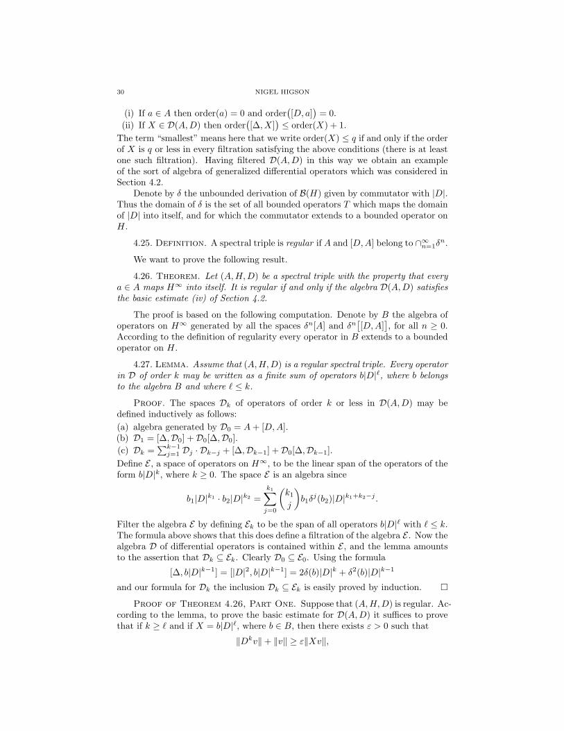
30 NIGEL HIGSON
(i) If a ∈ A then order(a) = 0 and order([D, a]
)= 0.
(ii) If X ∈ D(A,D) then order([∆, X]
)≤ order(X) + 1.
The term “smallest” means here that we write order(X) ≤ q if and only if the orderof X is q or less in every filtration satisfying the above conditions (there is at leastone such filtration). Having filtered D(A,D) in this way we obtain an exampleof the sort of algebra of generalized differential operators which was considered inSection 4.2.
Denote by δ the unbounded derivation of B(H) given by commutator with |D|.Thus the domain of δ is the set of all bounded operators T which maps the domainof |D| into itself, and for which the commutator extends to a bounded operator onH.
4.25. Definition. A spectral triple is regular if A and [D,A] belong to ∩∞n=1δn.
We want to prove the following result.
4.26. Theorem. Let (A,H,D) be a spectral triple with the property that everya ∈ A maps H∞ into itself. It is regular if and only if the algebra D(A,D) satisfiesthe basic estimate (iv) of Section 4.2.
The proof is based on the following computation. Denote by B the algebra ofoperators on H∞ generated by all the spaces δn[A] and δn
[[D,A]
], for all n ≥ 0.
According to the definition of regularity every operator in B extends to a boundedoperator on H.
4.27. Lemma. Assume that (A,H,D) is a regular spectral triple. Every operatorin D of order k may be written as a finite sum of operators b|D|`, where b belongsto the algebra B and where ` ≤ k.
Proof. The spaces Dk of operators of order k or less in D(A,D) may bedefined inductively as follows:(a) algebra generated by D0 = A+ [D,A].(b) D1 = [∆,D0] +D0[∆,D0].(c) Dk =
∑k−1j=1 Dj · Dk−j + [∆,Dk−1] +D0[∆,Dk−1].
Define E , a space of operators on H∞, to be the linear span of the operators of theform b|D|k, where k ≥ 0. The space E is an algebra since
b1|D|k1 · b2|D|k2 =k1∑j=0
(k1
j
)b1δ
j(b2)|D|k1+k2−j .
Filter the algebra E by defining Ek to be the span of all operators b|D|` with ` ≤ k.The formula above shows that this does define a filtration of the algebra E . Now thealgebra D of differential operators is contained within E , and the lemma amountsto the assertion that Dk ⊆ Ek. Clearly D0 ⊆ E0. Using the formula
[∆, b|D|k−1] = [|D|2, b|D|k−1] = 2δ(b)|D|k + δ2(b)|D|k−1
and our formula for Dk the inclusion Dk ⊆ Ek is easily proved by induction.
Proof of Theorem 4.26, Part One. Suppose that (A,H,D) is regular. Ac-cording to the lemma, to prove the basic estimate for D(A,D) it suffices to provethat if k ≥ ` and if X = b|D|`, where b ∈ B, then there exists ε > 0 such that
‖Dkv‖+ ‖v‖ ≥ ε‖Xv‖,

THE RESIDUE INDEX THEOREM OF CONNES AND MOSCOVICI 31
for every v ∈ H∞. But we have
‖Xv‖ = ‖b|D|`v‖ ≤ ‖b‖ · ‖|D|`v‖ = ‖b‖ · ‖D`v‖,And since by spectral theory for every ` ≤ k we have that
‖D`v‖2 ≤ ‖Dkv‖2 + ‖v‖2 ≤(‖Dkv‖+ ‖v‖
)2
it follows that‖Dkv‖+ ‖v‖ ≥ 1
‖b‖+ 1‖Xv‖,
as required.
To prove the converse, we shall develop a pseudodifferential calculus, as follows.
4.28. Definition. Let (A,H,D) be a spectral triple for which A ·H∞ ⊆ H∞,and for which the basic elliptic estimate holds. Fix an operator K : H∞ → H∞
of order −∞ and such that ∆1 = ∆ + K is invertible. A basic pseudodifferentialoperator of order k ∈ Z is a linear operator T : H∞ → H∞ with the property thatfor every ` ∈ Z the operator T may be decomposed as
T = X∆m21 +R,
where X ∈ D(A,D), m ∈ Z, and R : H∞ → H∞, and where
order(X) +m ≤ k and order(R) ≤ `.
A pseudodifferential operator of order k ∈ Z is a finite linear combination of basicpseudodifferential operators of order k.
4.29. Remarks. Every pseudodifferential operator is a sum of two basic oper-ators (one with the integer m in Definition 4.28 even, and one with m odd). Theclass of pseudodifferential operators does not depend on the choice of operator K.
4.30. Lemma. If T is a pseudodifferential operator and z ∈ C then
[∆z1, T ] ≈
∞∑j=1
(z
j
)T (j)∆z−j
1 .
Proof. See the proof of Lemma 4.20.
4.31. Proposition. The set of all pseudodifferential operators is a filtered alge-bra. If T is a pseudodifferential operator then so is δ(T ), and moreover order(δ(T )) ≤order(T ).
Proof. The set of pseudodifferential operators is a vector space. The formula
X∆m21 · Y∆
n21 ≈
∞∑j=0
(m2
j
)XY (j)∆
m+n2 −j
1
shows that it is closed under multiplication. Finally,
δ(T ) = |D|T − T |D| ≈ ∆121 T −∆
121 T
≈∞∑j=1
( 12
j
)T (j)∆
12−j1 .
This computation reduces the second part of the lemma to the assertion that ifT is a pseudodifferential operator of order k then T (1) = [∆, T ] is a pseudodiffer-ential operator of order k + 1 or less. This in turn follows from the definition of

32 NIGEL HIGSON
pseudodifferential operator and the fact that if X is a differential operator then thedifferential operator [∆, X] has order at most one more than the order of X.
Proof of Theorem 4.26, Part Two. Suppose that (A,H,D) is a spectraltriple for which A ·H∞ ⊆ H∞ and for which the basic estimate holds. By the basicestimate, every pseudodifferential operator of order zero extends to a boundedoperator on H. Since every operator in A or [D,A] is pseudodifferential of orderzero, and since δ(T ) is pseudodifferential of order zero whenever T is, we see thatif b ∈ A or b ∈ [D,A] then for every n the operator δn(b) extends to a boundedoperator on H. Hence the spectral triple (A,H,D) is regular, as required.
4.32. Definition. A spectral triple (A,H,D) is finitely summable if there is aSchatten ideal Lp(H) (where 1 ≤ p <∞)) such that
a · (1 +D2)−12 ∈ Lp(H)
for every a ∈ A.
If the spectral triple (A,H,D) is regular and finitely summable then for everyX ∈ D(A,D) the zeta function Trace(X∆− z
2 ) is defined in a right half-plane in C,and is holomorphic there. The following concept has been introduced by Connesand Moscovici [12, Definition II.1].
4.33. Definition. Let (A,H,D) be a regular and finitely summable spectraltriple. It has discrete dimension spectrum if9 there is a discrete subset F of C withthe following property: for every operator X in D(A,D) if order(X) ≤ q then thezeta function Trace(X∆− z
2 ) extends to a meromorphic function on C with all polescontained in F + q. The dimension spectrum of (A,H,D) is then the smallest suchset F .
4.34. Remark. The definition above extends without change to arbitrary al-gebras of generalized differential operators, and at one point (in Section 6) we shalluse it in this context.
A final item of terminology: in Appendix A we shall make use of the followingnotion:
4.35. Definition. A regular and finitely summable spectral triple has simpledimension spectrum if it has discrete dimension spectrum and if all the zeta-typefunctions above have only simple poles.
5. The Residue Cocycle
In this section we shall assume as given an algebra D(∆), a square root D of ∆,and an algebra A ⊆ D(∆), as in the previous sections. We shall assume the finiteanalytic dimension and analytic continuation properties set forth in Definitions 4.8and 4.11. We shall also assume that the Hilbert space H is nontrivially Z/2-gradedand therefore that the operator D has odd grading-degree. This is the “even-dimensional” case. The “odd-dimensional” case, where H has no grading, will beconsidered separately in Section 7.4.
9Connes and Moscovici add a technical condition concerning decay of zeta functions alongvertical lines in C; compare Appendix A.
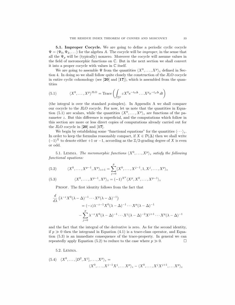
THE RESIDUE INDEX THEOREM OF CONNES AND MOSCOVICI 33
5.1. Improper Cocycle. We are going to define a periodic cyclic cocycleΨ = (Ψ0,Ψ2, . . . ) for the algebra A. The cocycle will be improper, in the sense thatall the Ψp will be (typically) nonzero. Moreover the cocycle will assume values inthe field of meromorphic functions on C. But in the next section we shall convertit into a proper cocycle with values in C itself.
We are going to assemble Ψ from the quantities 〈X0, . . . , Xp〉z defined in Sec-tion 4. In doing so we shall follow quite closely the construction of the JLO cocyclein entire cyclic cohomology (see [20] and [17]), which is assembled from the quan-tities
(5.1) 〈X0, . . . , Xp〉JLO = Trace(∫
Σp
εX0e−t0∆ . . . Xpe−tp∆ dt
)(the integral is over the standard p-simplex). In Appendix A we shall compareour cocycle to the JLO cocycle. For now, let us note that the quantities in Equa-tion (5.1) are scalars, while the quantities 〈X0, . . . , Xp〉z are functions of the pa-rameter z. But this difference is superficial, and the computations which follow inthis section are more or less direct copies of computations already carried out forthe JLO cocycle in [20] and [17].
We begin by establishing some “functional equations” for the quantities 〈· · · 〉z.In order to keep the formulas reasonably compact, if X ∈ D(∆) then we shall write(−1)X to denote either +1 or −1, according as the Z/2-grading degree of X is evenor odd.
5.1. Lemma. The meromorphic functions 〈X0, . . . , Xp〉z satisfy the followingfunctional equations:
〈X0, . . . , Xp−1, Xp〉z+1 =p∑j=0
〈X0, . . . , Xj−1, 1, Xj , . . . , Xp〉z(5.2)
〈X0, . . . , Xp−1, Xp〉z = (−1)Xp
〈Xp, X0, . . . , Xp−1〉z(5.3)
Proof. The first identity follows from the fact that
d
dλ
(λ−zX0(λ−∆)−1 · · ·Xp(λ−∆)−1
)= (−z)λ−z−1X0(λ−∆)−1 · · ·Xp(λ−∆)−1
−p∑j=0
λ−zX0(λ−∆)−1 · · ·Xj(λ−∆)−2Xj+1 · · ·Xp(λ−∆)−1
and the fact that the integral of the derivative is zero. As for the second identity,if p 0 then the integrand in Equation (4.1) is a trace-class operator, and Equa-tion (5.3) is an immediate consequence of the trace-property. In general we canrepeatedly apply Equation (5.2) to reduce to the case where p 0.
5.2. Lemma.
(5.4) 〈X0, . . . , [D2, Xj ], . . . , Xp〉z =
〈X0, . . . , Xj−1Xj , . . . Xp〉z − 〈X0, . . . , XjXj+1, . . . Xp〉z

34 NIGEL HIGSON
Proof. This follows from the identity
Xj−1(λ−∆)−1[D2, Xj ](λ−∆)−1Xj+1
= Xj−1(λ−∆)−1XjXj+1 −Xj−1Xj(λ−∆)−1Xj+1.
Note that when j = p equation (5.4) should read as
〈X0, . . . , Xp−1, [D2, Xp]〉z = 〈X0, . . . , Xp−1Xp〉z − (−1)Xp
〈XpX0, . . . , Xp−1〉z.
5.3. Lemma.
(5.5)p∑j=0
(−1)X0···Xj−1
〈X0, . . . , [D,Xj ], . . . , Xp〉z = 0
Proof. The identity is equivalent to the formula
Trace(ε[D,
∫λ−zX0(λ−∆)−1 · · ·Xp(λ−∆)−1 dλ
])= 0,
which holds since the supertrace of any (graded) commutator is zero.
With these preliminaries out of the way we can obtain very quickly the (im-proper) (b, B)-cocycle which is the main object of study in these notes.
5.4. Definition. If p is a non-negative and even integer then define a (p+ 1)-multi-linear functional on A with values in the meromorphic functions on C by theformula
Ψp(a0, . . . , ap) = 〈a0, [D, a1], . . . , [D, ap]〉s− p2
5.5. Theorem. The even (b, B)-cochain Ψ = (Ψ0,Ψ2,Ψ4 · · · ) is an (improper)(b, B)-cocycle.
Proof. First of all, it follows from the definition of B and Lemma 5.1 that
BΨp+2(a0, . . . , ap+1) =p+1∑j=0
(−1)j〈1, [D, aj ], . . . , [D, aj−1]〉s− p+22
=p+1∑j=0
〈[D, a0], . . . , [D, aj−1], 1, [D, aj ], . . . , [D, ap+1]〉s− p+22
= 〈[D, a0], [D, a1], . . . , [D, ap+1]〉s− p2.
Next, it follows from the definition of b and the Leibniz rule [D, ajaj+1] = aj [D, aj+1]+[D, aj ]aj+1 that
bΨp(a0, . . . , ap+1) =(〈a0a1, [D, a2], . . . , [D, ap+1]〉s− p
2
− 〈a0, a1[D, a2], . . . , [D, ap+1]〉s− p2
)−
(〈a0, [D, a1]a2, [D, a3], . . . , [D, ap+1]〉s− p
2
− 〈a0, [D, a1], a2[D, a3], . . . , [D, ap+1]〉s− p2
)+ · · ·+
(〈a0, [D, a1], . . . , [D, ap]ap+1〉s− p
2
− 〈ap+1a0, [D, a1], . . . , [D, ap+1]〉s− p2
).

THE RESIDUE INDEX THEOREM OF CONNES AND MOSCOVICI 35
Applying Lemma 5.2 we get
bΨp(a0, . . . , ap+1) =p+1∑j=1
(−1)j−1〈a0, [D, a1], . . . , [D2, aj ], . . . , [D, ap+1]〉s− p2
Setting X0 = a0 and Xj = [D, aj ] for j ≥ 1, and applying Lemma 5.3 we get
BΨp+2(a0, . . . , ap+1) + bΨp(a0, . . . , ap+1)
=p+1∑j=0
(−1)X0···Xj−1
〈X0, . . . , [D,Xj ], . . . , Xp+1〉s− p2
= 0.
5.2. Residue Cocycle. By taking residues at s = 0 we map the space ofmeromorphic functions on C to the scalar field C, and we obtain from any (b, B)-cocycle with coefficients in the space of meromorphic functions a (b, B)-cocyclewith coefficients in C. This operation transforms the improper cocycle Ψ that weconstructed in the last section into a proper cocycle Ress=0 Ψ. Indeed, it followsfrom Proposition 4.14 that if p is greater than the analytic dimension d of D(∆)then the function
Ψp(a0, . . . , ap)s = 〈a0, [D, a1], . . . , [D, ap]〉s− p2
is holomorphic at s = 0.The following proposition identifies the proper (b, B)-cocycle Ress=0 Ψ with the
residue cocycle studied by Connes and Moscovici.
5.6. Theorem. For all p ≥ 0 and all a0, . . . , ap ∈ A,
Ress=0 Ψp(a0, . . . , ap)
=∑k≥0
cp,k Ress=0 Tr(εa0[D, a1](k1) · · · [D, ap](kp)∆− p
2−|k|−s).
The sum is over all multi-indices (k1, . . . , kp) with non-negative integer entries, andthe constants cpk are given by the formula
cpk =(−1)k
k!Γ(|k|+ p
2 )(k1 + 1)(k1 + k2 + 2) · · · (k1 + · · ·+ kp + p)
5.7. Remarks. Before proving the theorem we need to make one or two com-ments about the above formula.
First, the constant c00 = Γ(0) is not well defined since 0 is a pole of the Γ-function. To cope with this problem we replace the term c00 Ress=0
(Tr(εa0∆−s)
)with Ress=0
(Γ(s)Tr(εa0∆−s)
).
Second, it follows from Proposition 4.14 that if |k| + p > d then the (p, k)-contribution to the above sum of residues is actually zero. Hence for every p thesum is in fact finite (and as we already noted above, the sum is 0 when p > d).
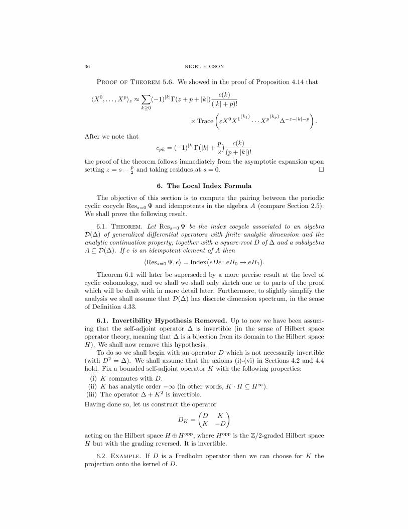
36 NIGEL HIGSON
Proof of Theorem 5.6. We showed in the proof of Proposition 4.14 that
〈X0, . . . , Xp〉z ≈∑k≥0
(−1)|k|Γ(z + p+ |k|) c(k)(|k|+ p)!
× Trace(εX0X1
(k1)· · ·Xp
(kp)∆−z−|k|−p
).
After we note that
cpk = (−1)|k|Γ(|k|+ p
2) c(k)(p+ |k|)!
the proof of the theorem follows immediately from the asymptotic expansion uponsetting z = s− p
2 and taking residues at s = 0.
6. The Local Index Formula
The objective of this section is to compute the pairing between the periodiccyclic cocycle Ress=0 Ψ and idempotents in the algebra A (compare Section 2.5).We shall prove the following result.
6.1. Theorem. Let Ress=0 Ψ be the index cocycle associated to an algebraD(∆) of generalized differential operators with finite analytic dimension and theanalytic continuation property, together with a square-root D of ∆ and a subalgebraA ⊆ D(∆). If e is an idempotent element of A then
〈Ress=0 Ψ, e〉 = Index(eDe : eH0 → eH1
).
Theorem 6.1 will later be superseded by a more precise result at the level ofcyclic cohomology, and we shall we shall only sketch one or to parts of the proofwhich will be dealt with in more detail later. Furthermore, to slightly simplify theanalysis we shall assume that D(∆) has discrete dimension spectrum, in the senseof Definition 4.33.
6.1. Invertibility Hypothesis Removed. Up to now we have been assum-ing that the self-adjoint operator ∆ is invertible (in the sense of Hilbert spaceoperator theory, meaning that ∆ is a bijection from its domain to the Hilbert spaceH). We shall now remove this hypothesis.
To do so we shall begin with an operator D which is not necessarily invertible(with D2 = ∆). We shall assume that the axioms (i)-(vi) in Sections 4.2 and 4.4hold. Fix a bounded self-adjoint operator K with the following properties:
(i) K commutes with D.(ii) K has analytic order −∞ (in other words, K ·H ⊆ H∞).(iii) The operator ∆ +K2 is invertible.Having done so, let us construct the operator
DK =(D KK −D
)acting on the Hilbert space H ⊕Hopp, where Hopp is the Z/2-graded Hilbert spaceH but with the grading reversed. It is invertible.
6.2. Example. If D is a Fredholm operator then we can choose for K theprojection onto the kernel of D.
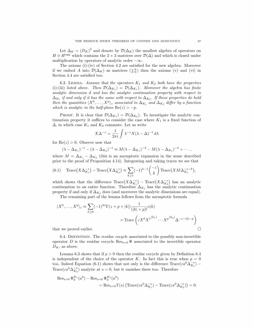
THE RESIDUE INDEX THEOREM OF CONNES AND MOSCOVICI 37
Let ∆K = (DK)2 and denote by D(∆K) the smallest algebra of operators onH ⊕Hopp which contains the 2× 2 matrices over D(∆) and which is closed undermultiplication by operators of analytic order −∞.
The axioms (i)-(iv) of Section 4.2 are satisfied for the new algebra. Moreoverif we embed A into D(∆K) as matrices ( a 0
0 0 ) then the axioms (v) and (vi) inSection 4.4 are satisfied too.
6.3. Lemma. Assume that the operators K1 and K2 both have the properties(i)-(iii) listed above. Then D(∆K1) = D(∆K1). Moreover the algebra has finiteanalytic dimension d and has the analytic continuation property with respect to∆K1 if and only if it has the same with respect to ∆K2 . If these properties do holdthen the quantities 〈X0, . . . , Xp〉z associated to ∆K1 and ∆K2 differ by a functionwhich is analytic in the half-plane Re(z) > −p.
Proof. It is clear that D(∆K1) = D(∆K2). To investigate the analytic con-tinuation property it suffices to consider the case where K1 is a fixed function of∆, in which case K1 and K2 commute. Let us write
X∆−z =1
2πi
∫λ−zX(λ−∆)−1 dλ
for Re(z) > 0. Observe now that
(λ−∆K1)−1 − (λ−∆K2)
−1 ≈M(λ−∆K1)−2 −M(λ−∆K1)
−3 + · · · ,where M = ∆K1 − ∆K2 (this is an asymptotic expansion in the sense describedprior to the proof of Proposition 4.14). Integrating and taking traces we see that
(6.1) Trace(X∆−z
K1
)− Trace
(X∆−z
K2
)≈
∑k≥1
(−1)k−1
(−zk
)Trace
(XM∆−z−k
K1
),
which shows that the difference Trace(X∆−z
K1
)− Trace
(X∆−z
K2
)has an analytic
continuation to an entire function. Therefore ∆K1 has the analytic continuationproperty if and only if ∆K2 does (and moreover the analytic dimensions are equal).
The remaining part of the lemma follows from the asymptotic formula
〈X0, . . . , Xp〉z ≈∑k≥0
(−1)|k|Γ(z + p+ |k|) 1(|k|+ p)!
c(k)
× Trace(εX0X1
(k1)· · ·Xp
(kp)∆−z−|k|−p
)that we proved earlier.
6.4. Definition. The residue cocycle associated to the possibly non-invertibleoperator D is the residue cocycle Ress=0 Ψ associated to the invertible operatorDK , as above.
Lemma 6.3 shows that if p > 0 then the residue cocycle given by Definition 6.4is independent of the choice of the operator K. In fact this is true when p = 0too. Indeed Equation (6.1) shows that not only is the difference Trace(εa0∆−s
K1)−
Trace(εa0∆−sK2
) analytic at s = 0, but it vanishes there too. Therefore
Ress=0 ΨK10 (a0)− Ress=0 ΨK2
0 (a0)
= Ress=0 Γ(s)(Trace(εa0∆−s
K1)− Trace(εa0∆−s
K2))
= 0.

38 NIGEL HIGSON
6.5. Example. If D happens to be invertible already then we obtain the sameresidue cocycle as before.
6.6. Example. In the case where D is Fredholm, the residue cocycle is givenby the same formula that we saw in Theorem 5.6:
Ress=0 Ψp(a0, . . . , ap)
=∑k≥0
cp,k Ress=0 Tr(εa0[D, a1](k1) · · · [D, ap](kp)∆− p
2−|k|−s).
The complex powers ∆−z are defined to be zero on the kernel of D (which is alsothe kernel of ∆). When p = 0 the residue cocycle is
Ress=0
(Γ(s) Trace(εao∆−s)
)+ Trace(εa0P ),
where the complex power ∆−s is defined as above and P is the orthogonal projectiononto the kernel of D.
6.2. Proof of the Index Theorem. Let us fix an idempotent e ∈ A anddefine a family of operators by the formula
Dt = D + t[e, [D, e]], t ∈ [0, 1].
Note that D0 = D while D1 = eDe + e⊥De⊥, so that in particular D1 commuteswith e. Denote by Ψt the improper cocycle associated to Dt (via the mechanismjust described in the last section which involves the incorporation of some order−∞ operator Kt, which we shall assume depends smoothly on t).
6.7. Lemma. Define an improper (b, B)-cochain Θt by the formula
Θtp(a
0, . . . , ap) =p∑j=0
(−1)j−1〈a0, . . . , [DKt, aj ], DKt
, [DKt, aj+1], . . . , [DKt
, ap]〉s− p+12,
where D = ddtDKt
∈ D(∆K). Then
BΘtp+1 + bΘt
p−1 +d
dtΨtp = 0.
The lemma, which is nothing more than an elaborate computation, can beproved by following the steps taken in Section 7.1 below (compare Remark 7.9).
Proof of Theorem 6.1. It follows from the asymptotic expansion methodused to prove Lemma 6.3 that each Ψt and each Θt is meromorphic. Since weare assuming that D(∆) has discrete dimension spectrum the poles of all thesefunctions are located within the same discrete set in C. As a result, the integral∫ 1
0Θt dt is clearly meromorphic too. Since
B
∫ 1
0
Θtp+1 dt+ b
∫ 1
0
Θtp−1 dt = Ψ0 −Ψ1,
it follows by taking residues that Ress=0 Ψ0 and Ress=1 Ψ1 are cohomologous. Asa result, we can compute the pairing 〈Ress=0 Ψ, e〉 using Ψ1 in place of Ψ0. Ifwe choose the operator K1 to commute with not only D1 but also e, then DK1
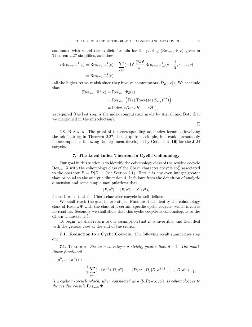
THE RESIDUE INDEX THEOREM OF CONNES AND MOSCOVICI 39
commutes with e and the explicit formula for the pairing 〈Ress=0 Ψ, e〉 given inTheorem 2.27 simplifies, as follows:
〈Ress=0 Ψ1, e〉 = Ress=0 Ψ10(e) +
∑k≥1
(−1)k(2k)!k!
Ress=0 Ψ12k(e−
12, e, . . . , e)
= Ress=0 Ψ10(e)
(all the higher terms vanish since they involve commutators [DK1 , e]). We concludethat
〈Ress=0 Ψ1, e〉 = Ress=0 Ψ10(e)
= Ress=0
(Γ(s)Trace(εe (∆K1)
−s))
= Index(eDe : eH0 → eH1
),
as required (the last step is the index computation made by Atiyah and Bott thatwe mentioned in the introduction).
6.8. Remark. The proof of the corresponding odd index formula (involvingthe odd pairing in Theorem 2.27) is not quite so simple, but could presumablybe accomplished following the argument developed by Getzler in [16] for the JLOcocycle.
7. The Local Index Theorem in Cyclic Cohomology
Our goal in this section is to identify the cohomology class of the residue cocycleRess=0 Ψ with the cohomology class of the Chern character cocycle chFn associatedto the operator F = D|D|−1 (see Section 2.1). Here n is any even integer greaterthan or equal to the analytic dimension d. It follows from the definition of analyticdimension and some simple manipulations that
[F, a0] · · · [F, an] ∈ L1(H),
for such n, so that the Chern character cocycle is well-defined.We shall reach the goal in two steps. First we shall identify the cohomology
class of Ress=0 Ψ with the class of a certain specific cyclic cocycle, which involvesno residues. Secondly we shall show that this cyclic cocycle is cohomologous to theChern character chFn .
To begin, we shall return to our assumption that D is invertible, and then dealwith the general case at the end of the section.
7.1. Reduction to a Cyclic Cocycle. The following result summarizes stepone.
7.1. Theorem. Fix an even integer n strictly greater than d − 1. The multi-linear functional
(a0, . . . , an) 7→
12
n∑j=0
(−1)j+1〈[D, a0], . . . , [D, aj ], D, [D, aj+1], . . . , [D, an]〉−n2.
is a cyclic n-cocycle which, when considered as a (b, B)-cocycle, is cohomologous tothe residue cocycle Ress=0 Ψ.

40 NIGEL HIGSON
7.2. Remark. It follows from Proposition 4.14 that the quantities
〈[D, a0], . . . , [D, aj ], D, [D, aj+1], . . . , [D, an]〉zwhich appear in the theorem are holomorphic in the half-plane Re(z) > −n
2 +1r (d − (n + 1)). Therefore it makes sense to evaluate them at z = −n
2 , as we havedone. Appearances might suggest otherwise, because the term Γ(z) which appearsin the definition of 〈. . . 〉z has poles at the non-positive integers (and in particularat z = −n
2 if n is even). However these poles are canceled by zeroes of the contourintegral in the given half-plane.
Theorem 7.1 and its proof have a simple conceptual explanation, which we shallgive in a little while (after Lemma 7.8). However a certain amount of elementary,if laborious, computation is also involved in the proof, and we shall get to work onthis first. For this purpose it is useful to introduce the following notation.
7.3. Definition. If X0, . . . , Xp are operators in the algebra generated byD(∆), 1 and D, and if at least one belongs to D(∆) then define
〈〈X0, . . . , Xp〉〉z =p∑k=0
(−1)X0···Xk
〈X0, . . . , Xk, D,Xk+1, . . . , Xp〉z,
which is a meromorphic function of z ∈ C.
The new notation allows us to write a compact formula for the cyclic cocycleappearing in Theorem 7.1:
(a0, . . . , an) 7→ 12 〈〈[D, a
0], . . . , [D, an]〉〉−n2.
We shall now list some properties of the quantities 〈〈· · · 〉〉z which are analogousto the properties of the quantities 〈· · · 〉z that we verified in Section 5. The followinglemma may be proved using the formulas in Lemmas 5.1 and 5.2.
7.4. Lemma. The quantity 〈〈X0, . . . , Xp〉〉z satisfies the following identities:
〈〈X0, . . . , Xp〉〉z = 〈〈Xp, X0, . . . , Xp−1〉〉z(7.1)p∑j=0
〈〈X0, . . . , Xj , 1, Xj+1, . . . , Xp〉〉z+1 = 〈〈X0, . . . , Xp〉〉z(7.2)
In addition,
(7.3) 〈〈X0, . . . , Xj−1Xj , . . . , Xp〉〉z − 〈〈X0, . . . , XjXj+1, . . . , Xp〉〉z
= 〈〈X0, . . . , [D2, Xj ], . . . , Xp〉〉z − (−1)X0···Xj−1
〈X0, . . . , [D,Xj ], . . . , Xp〉z.
(In both instances within this last formula the commutators are graded commuta-tors.)
7.5. Remark. When j = p equation (7.3) should be read as
〈〈X0, . . . , Xp−1Xp〉〉z − 〈〈XpX0, . . . , Xp−1〉〉z
= 〈〈X0, . . . , Xp−1, [D2, Xp]〉〉z − (−1)X0···Xp−1
〈X0, . . . , Xp−1, [D,Xp]〉z.
We shall also need a version of Lemma 5.3, as follows.
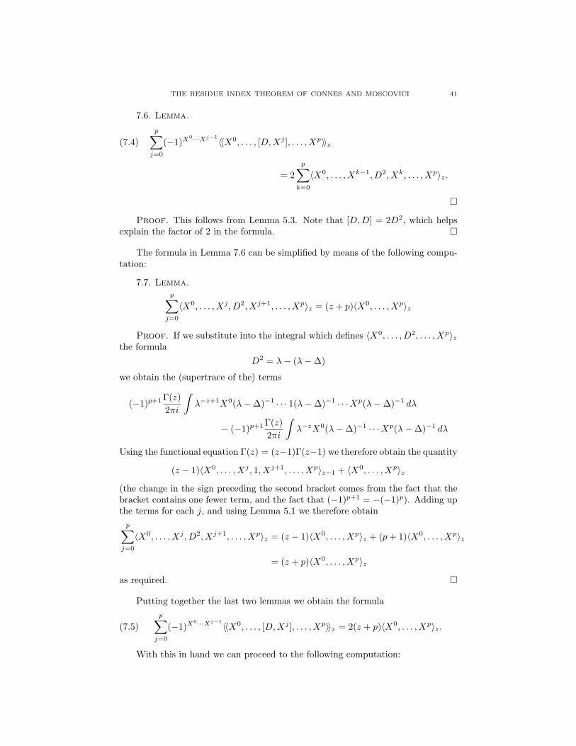
THE RESIDUE INDEX THEOREM OF CONNES AND MOSCOVICI 41
7.6. Lemma.
(7.4)p∑j=0
(−1)X0···Xj−1
〈〈X0, . . . , [D,Xj ], . . . , Xp〉〉z
= 2p∑k=0
〈X0, . . . , Xk−1, D2, Xk, . . . , Xp〉z.
Proof. This follows from Lemma 5.3. Note that [D,D] = 2D2, which helpsexplain the factor of 2 in the formula.
The formula in Lemma 7.6 can be simplified by means of the following compu-tation:
7.7. Lemma.p∑j=0
〈X0, . . . , Xj , D2, Xj+1, . . . , Xp〉z = (z + p)〈X0, . . . , Xp〉z
Proof. If we substitute into the integral which defines 〈X0, . . . , D2, . . . , Xp〉zthe formula
D2 = λ− (λ−∆)
we obtain the (supertrace of the) terms
(−1)p+1 Γ(z)2πi
∫λ−z+1X0(λ−∆)−1 · · · 1(λ−∆)−1 · · ·Xp(λ−∆)−1 dλ
− (−1)p+1 Γ(z)2πi
∫λ−zX0(λ−∆)−1 · · ·Xp(λ−∆)−1 dλ
Using the functional equation Γ(z) = (z−1)Γ(z−1) we therefore obtain the quantity
(z − 1)〈X0, . . . , Xj , 1, Xj+1, . . . , Xp〉z−1 + 〈X0, . . . , Xp〉z
(the change in the sign preceding the second bracket comes from the fact that thebracket contains one fewer term, and the fact that (−1)p+1 = −(−1)p). Adding upthe terms for each j, and using Lemma 5.1 we therefore obtainp∑j=0
〈X0, . . . , Xj , D2, Xj+1, . . . , Xp〉z = (z − 1)〈X0, . . . , Xp〉z + (p+ 1)〈X0, . . . , Xp〉z
= (z + p)〈X0, . . . , Xp〉z
as required.
Putting together the last two lemmas we obtain the formula
(7.5)p∑j=0
(−1)X0···Xj−1
〈〈X0, . . . , [D,Xj ], . . . , Xp〉〉z = 2(z + p)〈X0, . . . , Xp〉z.
With this in hand we can proceed to the following computation:
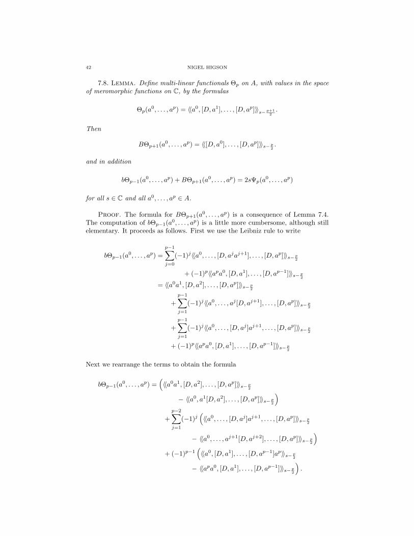
42 NIGEL HIGSON
7.8. Lemma. Define multi-linear functionals Θp on A, with values in the spaceof meromorphic functions on C, by the formulas
Θp(a0, . . . , ap) = 〈〈a0, [D, a1], . . . , [D, ap]〉〉s− p+12.
Then
BΘp+1(a0, . . . , ap) = 〈〈[D, a0], . . . , [D, ap]〉〉s− p2.
and in addition
bΘp−1(a0, . . . , ap) +BΘp+1(a0, . . . , ap) = 2sΨp(a0, . . . , ap)
for all s ∈ C and all a0, . . . , ap ∈ A.
Proof. The formula for BΘp+1(a0, . . . , ap) is a consequence of Lemma 7.4.The computation of bΘp−1(a0, . . . , ap) is a little more cumbersome, although stillelementary. It proceeds as follows. First we use the Leibniz rule to write
bΘp−1(a0, . . . , ap) =p−1∑j=0
(−1)j〈〈a0, . . . , [D, ajaj+1], . . . , [D, ap]〉〉s− p2
+ (−1)p〈〈apa0, [D, a1], . . . , [D, ap−1]〉〉s− p2
= 〈〈a0a1, [D, a2], . . . , [D, ap]〉〉s− p2
+p−1∑j=1
(−1)j〈〈a0, . . . , aj [D, aj+1], . . . , [D, ap]〉〉s− p2
+p−1∑j=1
(−1)j〈〈a0, . . . , [D, aj ]aj+1, . . . , [D, ap]〉〉s− p2
+ (−1)p〈〈apa0, [D, a1], . . . , [D, ap−1]〉〉s− p2
Next we rearrange the terms to obtain the formula
bΘp−1(a0, . . . , ap) =(〈〈a0a1, [D, a2], . . . , [D, ap]〉〉s− p
2
− 〈〈a0, a1[D, a2], . . . , [D, ap]〉〉s− p2
)+p−2∑j=1
(−1)j(〈〈a0, . . . , [D, aj ]aj+1, . . . , [D, ap]〉〉s− p
2
− 〈〈a0, . . . , aj+1[D, aj+2], . . . , [D, ap]〉〉s− p2
)+ (−1)p−1
(〈〈a0, [D, a1], . . . , [D, ap−1]ap〉〉s− p
2
− 〈〈apa0, [D, a1], . . . , [D, ap−1]〉〉s− p2
).

THE RESIDUE INDEX THEOREM OF CONNES AND MOSCOVICI 43
We can now apply Lemma 7.6:
bΘp−1(a0, . . . , ap) =(〈〈a0, [D2, a1], [D, a2], . . . , [D, ap]〉〉s− p
2
+ 〈a0, [D, a1], [D, a2], . . . , [D, ap]〉s− p2
)+p−2∑j=1
(−1)j(〈〈a0, [D, a1], . . . , [D2, aj+1], . . . , [D, ap]〉〉s− p
2
+ (−1)j 〈a0, [D, a1], . . . , [D, aj+1], . . . , [D, ap]〉s− p2
)+ (−1)p−1
(〈〈a0, [D, a1], . . . , [D, ap−1], [D2, ap]〉〉s− p
2
+ (−1)p−1〈a0, [D, a1], . . . , [D, ap−1], [D, ap]〉s− p2
).
Collecting terms we get
bΘp−1(a0, . . . , ap) =p∑k=1
(−1)k−1〈〈a0, [D, a1], . . . , [D2, ak], . . . , [D, ap]〉〉s− p2
+ p〈a0, [D, a1], . . . , [D, ap]〉s− p2.
All that remains now is to add together bΘ and BΘ, and apply Equation (7.5) tothe result. Writing a0 = X0 and [D, aj ] = Xj for j = 1, . . . , p we get
bΘp−1(a0, . . . , ap) +BΘp+1(a0, . . . , ap)
=p∑j=0
(−1)X0···Xj−1
〈〈X0, . . . , [D,Xj ], . . . , Xp〉〉s− p2− p〈X0, . . . , Xp〉s− p
2
= 2(s− p
2+ p)〈X0, . . . , Xp〉s− p
2− p〈X0, . . . , Xp〉s− p
2
= 2s〈X0, . . . , Xp〉s− p2,
as the lemma requires.
7.9. Remark. The statement of Lemma 7.8 can be explained as follows. If wereplace D by tD and ∆ by t2∆ in the definitions of 〈· · · 〉z and Ψp, so as to obtaina new improper (b, B)-cocycle Ψt = (Ψt
0,Ψt2, . . . ), then it is easy to check from the
definitions thatΨtp(a
0, . . . , ap) = t−2sΨp(a0, . . . , ap).
Now, we expect that as t varies the cohomology class of the cocycle Ψt should notchange. And indeed, by borrowing known formulas from the theory of the JLOcocycle (see for example [17], or [18, Section 10.2], or Section 6 below) we canconstruct a (b, B)-cochain Θ such that
BΘ + bΘ +d
dtΨt = 0.
This is the same Θ as that which appears in the lemma.
The proof of Theorem 7.1 is now very straightforward:
Proof of Theorem 7.1. According to Lemma 7.8 the (b, B)-cochain(Ress=0
( 12s
Θ1
),Ress=0
( 12s
Θ3
), . . . ,Ress=0
( 12s
Θn−1
), 0, 0, . . .
)

44 NIGEL HIGSON
cobounds the difference of Ress=0 Ψ and the cyclic n-cocycle Ress=0
(12sBΘn+1
).
Since
Ress=0
( 12sBΘn+1
)(a0, . . . , an) =
12〈〈[D, a0], . . . , [D, an]〉〉−n
2
the theorem is proved.
7.2. Computation with the Cyclic Cocycle. We turn now to the secondstep. We are going to alter D by means of the following homotopy:
Dt = D|D|−t (0 ≤ t ≤ 1)
(the same strategy is employed by Connes and Moscovici in [10]). We shall similarlyreplace ∆ with ∆t = D2
t , and we shall use ∆t in place of ∆ in the definitions of〈· · · 〉z and of 〈〈· · · 〉〉z.
To simplify the notation we shall drop the subscript t in the following com-putation and denote by D = −Dt · log |D| the derivative of the operator Dt withrespect to t.
7.10. Lemma. Define a multi-linear functional on A, with values in the analyticfunctions on the half-plane Re(z) + n > d−1
2 , by the formula
Φtn(a0, . . . , an) = 〈〈a0D, [D, a1], . . . , [D, an]〉〉z.
Then BΦtn is a cyclic (n− 1)-cochain and
bBΦtn(a0, . . . , an)
=d
dt〈〈[D, a0], . . . , [D, an]〉〉z + (2z + n)
n∑j=0
〈D, [D, aj ], . . . , [Dj−1]〉z.
7.11. Remark. Observe that the operator log |D| has analytic order δ or less,for every δ > 0. As a result, the proof of Proposition 4.14 shows that the quantityis a holomorphic function of z in the half-plane Re(z) + n > d−1
2 . But we shall notbe concerned with any possible meromorphic continuation to C.
Proof. Let us take advantage of the fact that bB+Bb = 0 and compute BbΦt
instead (fewer minus signs and wrap-around terms are involved).A straightforward application of the definitions in Section 2 shows that the
quantity BbΦtn(a0, . . . , an) is the sum, from j = 0 to j = n, of the following terms:
− 〈〈D, [D, ajaj+1], [D, aj+2], . . . , [D, aj−1]〉〉z+ 〈〈D, [D, aj ], [D, aj+1aj+2], . . . , [D, aj−1]〉〉z− · · ·
+ (−1)n〈〈D, [D, aj ], [D, aj+1], . . . , [D, aj−2aj−1]〉〉z.
If we add the term 〈〈Daj , [D, aj+1], . . . , [D, aj−1〉〉z to the beginning of this expres-sion, and also the terms
− 〈〈aj−1D, [D, ajaj+1], [D, aj+2], . . . , [D, aj−2]〉〉z− 〈〈[D, aj ], [D, aj+1], . . . , [D, aj−1]〉〉z
at the end, then, after summing over all j, we have added zero in total. But we cannow invoke Leibniz’s rule to expand [D, akak+1] and apply part (iii) of Lemma 7.4

THE RESIDUE INDEX THEOREM OF CONNES AND MOSCOVICI 45
to obtain the quantity(〈〈D, [D2, aj ], [D, aj+2], . . . , [D, aj−1]〉〉z
− 〈〈D, [D, aj ], [D2, aj+1], . . . , [D, aj−1]〉〉z+ . . .
+(−1)n〈〈D, [D, aj ], [D, aj+1], . . . , [D2, aj−1]〉〉z)
+ (n+ 1)〈D, [D, aj ], [D, aj+1], . . . , [D, aj−1]〉z− 〈〈[D, aj ], [D, aj+1], . . . , [D, aj−1]〉〉z
(summed over j, as before). Applying Equation 7.5 we arrive at the followingformula
BbΦtn(a0, . . . , an) =
∑nj=0〈〈[D, D], [D, aj ], [D, aj+2], . . . , [D, aj−1]〉〉z
− (2z + (n+ 1))∑nj=0〈D, [D, a
j ], . . . , [D, aj−1]〉z−
∑nj=0〈〈[D, a
j ], [D, aj+1], . . . , [D, aj−1]〉〉z.
To complete the proof we write
〈〈[D, a0], . . . , [D, ap]〉〉z =∑nj=0〈D, [D, a
j ], . . . , [D, aj−1]〉z
and differentiate with respect to t, bearing in mind the definition of the quantities〈. . . 〉z and the fact that d
dt (λ−∆)−1 = (λ−∆)−1[D, D](λ−∆)−1. We obtain
ddt 〈〈[D, a
0], . . . , [D, ap]〉〉z = −∑nj=0〈〈[D, D], [D, aj ], [D, aj+2], . . . , [D, aj−1]〉〉z
+∑nj=0〈D, [D, a
j ], . . . , [D, aj−1]〉z+
∑nj=0〈〈[D, a
j ], [D, aj+1], . . . , [D, aj−1]〉〉z.
This proves the lemma.
We can now complete the second step, and with it the proof of the Connes-Moscovici Residue Index Theorem:
7.12. Theorem (Connes and Moscovici). The residue cocycle Ress=0 Ψ is co-homologous, as a (b, B)-cocycle, to the Chern character cocycle of Connes.
Proof. Thanks to Theorem 7.1 it suffices to show that the cyclic cocycle
(7.6)12〈〈[D, a0], . . . , [D, an]〉〉−n
2
is cohomologous to the Chern character. To do this we use the homotopy Dt above.Thanks to Lemma 7.10 the coboundary of the cyclic cochain∫ 1
0
BΨtn(a
0, . . . , an−1) dt

46 NIGEL HIGSON
is the difference of the cocycles (7.6) associated to D0 = D and D1 = F . For D1
we have D21 = ∆1 = I and so
12〈〈[D1, a
0], . . . , [D1, an]〉〉z
=12
n∑j=1
(−1)j+1 (−1)n+1Γ(z)2πi
×
Trace(∫
λ−zε[F, a0] · · · [F, aj ]F · · · [F, an](λ− I)−(n+2) dλ
)Since F anticommutes with each operator [F, aj ] this simplifies to
12
n∑j=1
(−1)n+1Γ(z)2πi
Trace(∫
λ−zεF [F, a0] · · · [F, an](λ− I)−(n+2) dλ
).
The terms in the sum are now all the same, and after applying Cauchy’s formulawe get
n+ 12
(−1)n+1Γ(z) · Trace(εF [F, a0] · · · [F, an]
)·(−zn+ 1
).
Using the functional equation for the Γ-function this reduces to
Γ(z + n+ 1)2 · n!
Trace(εF [F, a0] · · · [F, an]
)and evaluating at z = −n
2 we obtain the Chern character of Connes.
7.3. Invertibility Hypothesis Removed. In the case whereD is non-invert-ible we employ the device introduced in Section 6.1, and associate to D the residuecocycle for the operator DK .
Now Connes’ Chern character cocycle is defined for a not necessarily invertibleoperator D by forming first DK , then FK = DK |DK |−1, then chFK
n . See [4, PartI]. The following result therefore follows immediately from our calculations in theinvertible case.
7.13. Theorem. For any operator D, invertible or not, the class in periodiccyclic cohomology of the residue cocycle Ress=0 Ψ is equal to the class of the Cherncharacter cocycle of Connes.
7.4. The Odd-Dimensional Case. We shall briefly indicate the changeswhich must be made to deal with the “odd” degree case, consisting of a self-adjointoperator D on a trivially graded Hilbert space H.
The basic definition of the quantity 〈· · · 〉z is unchanged, except of course thatnow we set ε = I, and so we could omit ε from Equation (4.1). The formula
Ψp(a0, . . . , ap) = 〈a0, [D, a1], . . . , [D, ap]〉s− p2
now defines an odd, improper cocycle, with values in the meromorphic functions onC. The proof of this is almost the same as the proof of Theorem 5.5. We obtain

THE RESIDUE INDEX THEOREM OF CONNES AND MOSCOVICI 47
the formula
(7.7) BΨp+2(a0, . . . , ap+1) + bΨp(a0, . . . , ap+1)
= 〈[D, a0], [D, a1], . . . , [D, ap+1]〉s− p2
+p+1∑j=1
(−1)j−1〈a0, [D, a1], . . . , [D2, aj ], . . . , [D, ap+1]〉s− p2,
as in that proof, but instead of appealing to Lemma 5.3 we now note that
[D2, aj ] = D[D, aj ] + [D, aj ]D
and〈· · · , [D, aj−1], D[D, aj ], . . . 〉z = 〈· · · , [D, aj−1]D, [D, aj ], . . . 〉z.
Using these relations the right hand side of Equation (7.7) telescopes to 0. Thecomputation of Ress=0 Ψ is unchanged from the proof of Theorem 5.6, except forthe omission of ε.
With similar modifications to the proofs of Lemmas 7.8 and 7.10 we obtainwithout difficulty the odd version of Theorem 7.12.
Appendix A. Comparison with the JLO Cocycle
In this appendix we shall use the residue theorem and the Mellin transform ofcomplex analysis to compare the residue cocycle with the JLO cocycle.
The JLO cocycle, discovered by Jaffe, Lesniewski and Osterwalder [20], wasdeveloped in the context of spectral triples, as in Section 4.5, and accordingly weshall begin with such a spectral triple (A,H,D). Since we are going to comparethe JLO cocycle with the residue cocycle we shall assume that (A,H,D) has theadditional properties considered in Section 4.5 (although the theory of the JLOcocycle itself can be developed in greater generality). Thus we shall assume that ourspectral triple is regular, is finitely summable, and has discrete dimension spectrum.We shall also make an additional assumption later on in this section.
We shall consider only the even, Z/2-graded case here, but the odd case canbe developed in exactly the same way.
A.1. Definition. If X0, . . . , Xp are bounded operators on H, and if t > 0, letus define
〈X0, . . . , Xp〉JLOt = t
p2 Trace
(∫Σp
εX0e−u0t∆ . . . Xpe−upt∆ du
)The integral is over the standard p-simplex
Σp =
(u0, . . . , up)∣∣∣uj ≥ 0 & u0 + · · ·+ up = 1
.
The JLO cocycle is the improper (b, B)-cocycle
(a0, . . . , ap) 7→ 〈a0, [D, a1], . . . , [D, ap]〉JLOt ,
which should be thought of here as a cocycle with coefficients in the space offunctions of t > 0.
Strictly speaking the “traditional” JLO cocycle is given by the above formula forthe particular value t = 1. Our formula for 〈a0, [D, a1], . . . , [D, ap]〉JLO
t correspondsto the traditional cocycle associated to the operator t
12D. It will be quite convenient
to think of the JLO cocycle as a function of t > 0.

48 NIGEL HIGSON
Of course, it is a basic result that the JLO cocycle really is a cocycle. See [20]or [17].
The proper context for the JLO cocycle is Connes’ entire cyclic cohomology [5,7] for Banach algebras. We shall not describe this theory here, except to say thatthere is a natural map
HCP ∗(A) → HCP ∗entire(A),and that the arguments which follow show that the image of the residue cocycle inentire cyclic cohomology is the JLO cocycle.10
The following formula (which is essentially due to Connes [6, Equation (17)])exhibits the connection between the JLO cocycle and the cocycle that we con-structed in Section 5.
A.2. Lemma. If p > 0 and if X0, . . . , Xp are generalized differential operatorsin D(A,D), then
〈X0, . . . , Xp〉JLOt
= t−p2(−1)p
2πiTrace
(∫e−tλεX0(λ−∆)−1X1 · · ·Xp(λ−∆)−1 dλ
).
As in Section 4.3 the contour integral should be evaluated along a (downwardpointing) vertical line in the complex plane which separates 0 from the spectrumof ∆. The hypotheses guarantee the absolute convergence of the integral, in thenorm-topology. The formula in the lemma is also correct for p = 0, but in this casethe integral has to be suitably interpreted since it does not converge in the ordinarysense.
Proof of the Lemma. For simplicity let us assume that the operators Xj
are bounded (this is the only case of the lemma that we shall use below).By Cauchy’s Theorem, we may replace the contour of integration along which
the contour integral is computed by the imaginary axis in C (traversed upward).Having done so we obtain the formula
(A.1)(−1)p
2πi
∫e−tλX0(λ−∆)−1X1 · · ·Xp(λ−∆)−1 dλ
=12π
∫ ∞
−∞eitvX0(iv + ∆)−1 · · ·Xp(iv + ∆)−1 dv.
Note that this has the appearance of an inverse Fourier transform. As for the JLOcocycle, if we define functions gj from R into the bounded operators on H by
u 7→
Xje−u∆ if u ≥ 0
0 if u < 0.
then we obtain the formula
(A.2) tp2
∫Σp
X0e−u0t∆ . . . Xpe−upt∆ du
= t−p2
∫ ∞
−∞· · ·
∫ ∞
−∞g0(t− u1)g1(u1 − u2) · · · gn−1(un−1 − un)gn(un) du1 . . . dun,
10This result can be improved somewhat. Entire cyclic cohomology is defined for locallyconvex algebras, and one can identify the JLO cocycle and the residue cocycle in the entire cyclic
cohomology of various completions of A.
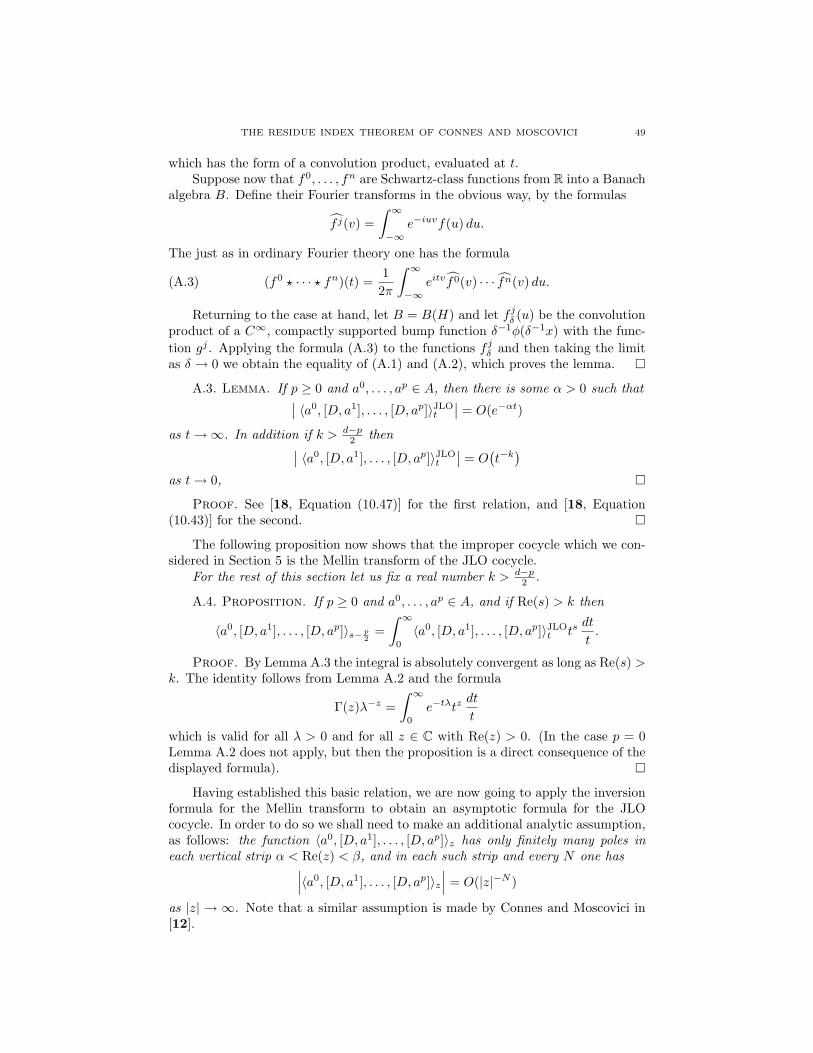
THE RESIDUE INDEX THEOREM OF CONNES AND MOSCOVICI 49
which has the form of a convolution product, evaluated at t.Suppose now that f0, . . . , fn are Schwartz-class functions from R into a Banach
algebra B. Define their Fourier transforms in the obvious way, by the formulas
f j(v) =∫ ∞
−∞e−iuvf(u) du.
The just as in ordinary Fourier theory one has the formula
(A.3) (f0 ? · · · ? fn)(t) =12π
∫ ∞
−∞eitv f0(v) · · · fn(v) du.
Returning to the case at hand, let B = B(H) and let f jδ (u) be the convolutionproduct of a C∞, compactly supported bump function δ−1φ(δ−1x) with the func-tion gj . Applying the formula (A.3) to the functions f jδ and then taking the limitas δ → 0 we obtain the equality of (A.1) and (A.2), which proves the lemma.
A.3. Lemma. If p ≥ 0 and a0, . . . , ap ∈ A, then there is some α > 0 such that∣∣ 〈a0, [D, a1], . . . , [D, ap]〉JLOt
∣∣ = O(e−αt)
as t→∞. In addition if k > d−p2 then∣∣ 〈a0, [D, a1], . . . , [D, ap]〉JLO
t
∣∣ = O(t−k
)as t→ 0,
Proof. See [18, Equation (10.47)] for the first relation, and [18, Equation(10.43)] for the second.
The following proposition now shows that the improper cocycle which we con-sidered in Section 5 is the Mellin transform of the JLO cocycle.
For the rest of this section let us fix a real number k > d−p2 .
A.4. Proposition. If p ≥ 0 and a0, . . . , ap ∈ A, and if Re(s) > k then
〈a0, [D, a1], . . . , [D, ap]〉s− p2
=∫ ∞
0
〈a0, [D, a1], . . . , [D, ap]〉JLOt ts
dt
t.
Proof. By Lemma A.3 the integral is absolutely convergent as long as Re(s) >k. The identity follows from Lemma A.2 and the formula
Γ(z)λ−z =∫ ∞
0
e−tλtzdt
t
which is valid for all λ > 0 and for all z ∈ C with Re(z) > 0. (In the case p = 0Lemma A.2 does not apply, but then the proposition is a direct consequence of thedisplayed formula).
Having established this basic relation, we are now going to apply the inversionformula for the Mellin transform to obtain an asymptotic formula for the JLOcocycle. In order to do so we shall need to make an additional analytic assumption,as follows: the function 〈a0, [D, a1], . . . , [D, ap]〉z has only finitely many poles ineach vertical strip α < Re(z) < β, and in each such strip and every N one has∣∣∣〈a0, [D, a1], . . . , [D, ap]〉z
∣∣∣ = O(|z|−N )
as |z| → ∞. Note that a similar assumption is made by Connes and Moscovici in[12].
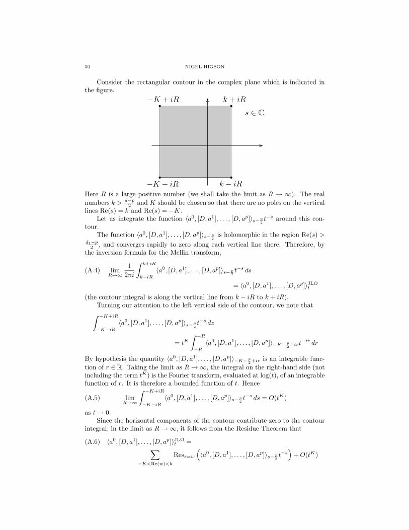
50 NIGEL HIGSON
Consider the rectangular contour in the complex plane which is indicated inthe figure.
−K − iR
k + iR−K + iR
k − iR
s ∈ C
Here R is a large positive number (we shall take the limit as R → ∞). The realnumbers k > d−p
2 and K should be chosen so that there are no poles on the verticallines Re(s) = k and Re(s) = −K.
Let us integrate the function 〈a0, [D, a1], . . . , [D, ap]〉s− p2t−s around this con-
tour.The function 〈a0, [D, a1], . . . , [D, ap]〉s− p
2is holomorphic in the region Re(s) >
d1−p2 , and converges rapidly to zero along each vertical line there. Therefore, by
the inversion formula for the Mellin transform,
(A.4) limR→∞
12πi
∫ k+iR
k−iR〈a0, [D, a1], . . . , [D, ap]〉s− p
2t−s ds
= 〈a0, [D, a1], . . . , [D, ap]〉JLOt
(the contour integral is along the vertical line from k − iR to k + iR).Turning our attention to the left vertical side of the contour, we note that∫ −K+iR
−K−iR〈a0, [D, a1], . . . , [D, ap]〉s− p
2t−s dz
= tK∫ −R
−R〈a0, [D, a1], . . . , [D, ap]〉−K− p
2 +irt−ir dr
By hypothesis the quantity 〈a0, [D, a1], . . . , [D, ap]〉−K− p2 +ir is an integrable func-
tion of r ∈ R. Taking the limit as R→∞, the integral on the right-hand side (notincluding the term tK) is the Fourier transform, evaluated at log(t), of an integrablefunction of r. It is therefore a bounded function of t. Hence
(A.5) limR→∞
∫ −K+iR
−K−iR〈a0, [D, a1], . . . , [D, ap]〉s− p
2t−s ds = O(tK)
as t→ 0.Since the horizontal components of the contour contribute zero to the contour
integral, in the limit as R→∞, it follows from the Residue Theorem that
(A.6) 〈a0, [D, a1], . . . , [D, ap]〉JLOt =∑
−K<Re(w)<k
Ress=w(〈a0, [D, a1], . . . , [D, ap]〉s− p
2t−s
)+O(tK)
THE RESIDUE INDEX THEOREM OF CONNES AND MOSCOVICI 51
as t→ 0.
A.5. Theorem. Assume that the spectral triple (A,H,D) is regular and hassimple dimension spectrum. Then for every p ≥ 0 and all a0, . . . ap ∈ A the quantity〈a0, [D, a1], . . . , [D, ap]〉JLO
t has an asymptotic expansion in powers of t as decreasesto zero. The residue cocycle Ress=0 Ψ(a0, . . . , ap) is the coefficient of the constantterm in this asymptotic expansion.
Appendix B. Complex Powers in a Differential Algebra
In this appendix we shall try to sketch out a more conceptual view of theimproper cocycle which was constructed in Section 5. This involves Quillen’scochain picture of cyclic cohomology [23], and in fact it was Quillen’s accountof the JLO cocycle from this perspective which first led to the formula for thequantity 〈X0, . . . , Xp〉z given in Definition 4.12.
We shall not attempt to carefully reconstruct the results of Sections 5 and 7from the cochain perspective, and in fact for the sake of brevity we shall disregardanalytic niceties altogether. Our purpose is only to set the main definitions of thesenotes against a background which may (or may not) make them seem more natural.
With this limited aim in mind we shall assume, as we did in the body of thenotes, that the operator ∆ is invertible. We shall also consider only the even case,in which the Hilbert space H on which ∆ acts is Z/2-graded.
As we did when we looked at cyclic cohomology in Section 2, let us fix analgebra A. But let us now also fix a second algebra L. For n ≥ 0 denote byHomn(A,L) the vector space of n-linear maps from A to L. By a 0-linear mapfrom A to L we shall mean a linear map from C to L, or in other words just anelement of L. Let Hom∗∗(A,L) be the direct product
Hom∗∗(A,L) =∞∏n=0
Homn(A,L).
Thus an element φ of Hom∗∗(A,L) is a sequence of multi-linear maps from A toL. We shall denote by φ(a1, . . . , an) the value of the n-th component of φ on then-tuple (a1, . . . , an).
The vector space Hom∗∗(A,L) is Z/2-graded in the following way: an elementφ is even (resp. odd) if φ(a1, . . . , an) = 0 for all odd n (resp. for all even n). Weshall denote by degM (φ) ∈ 0, 1 the grading-degree of φ. (The letter “M” standsfor “multi-linear;” a second grading-degree will be introduced below.)
B.1. Lemma. If φ, ψ ∈ Hom∗∗(A,L), then define
φ ∨ ψ(a1, . . . , an) =∑
p+q=n
φ(a1, . . . , ap)ψ(ap+1, . . . , an)
and
dMφ(a1, . . . , an+1) =n∑i=1
(−1)i+1φ(a1, . . . , aiai+1, . . . , an+1).
The vector space Hom∗∗(A,L), so equipped with a multiplication and differential,is a Z/2-graded differential algebra.
Let us now suppose that the algebra L is Z/2-graded. If φ ∈ Hom∗∗(A,L) thenlet us write degL(φ) = 0 if φ(a1, . . . , an) belongs to the degree-zero part of L forevery n and every n-tuple (a1, . . . , an). Similarly, if φ ∈ Hom∗∗(A,L) then let us

52 NIGEL HIGSON
write degL(φ) = 1 if φ(a1, . . . , an) belongs to the degree-one part of L for everyn and every n-tuple (a1, . . . , an). This is a new Z/2-grading on the vector spaceHom∗∗(A,L). The formula
deg(φ) = degM (φ) + degL(φ)
defines a third Z/2-grading—the one we are really interested in. Using this lastZ/2-grading, we have the following result:
B.2. Lemma. If φ, ψ ∈ Hom∗∗(A,L), then define
φ ψ = (−1)degM (φ) degL(ψ)φ ∨ ψ
anddφ = (−1)degL(φ)d′φ
These new operations once again provide Hom∗∗(A,L) with the structure of a Z/2-graded differential algebra (for the total Z/2-grading deg(φ) = degM (φ)+degL(φ)).
We shall now specialize to the following situation: A will be, as in Section 5, analgebra of differential order zero and grading degree zero operators contained withinan algebra D(∆) of generalized differential operators, and L will be the algebra ofall operators on the Z/2-graded vector space H∞ ⊆ H.
Denote by ρ the inclusion of A into L. This is of course a 1-linear map from Ato L, and we can therefore think of ρ as an element of Hom∗∗(A,L) (all of whosen-linear components are zero, except for n = 1).
Denote by D a square root of ∆, as in Section 4.4. Think of D as a 0-linearmap from A to L, and therefore as an element of Hom∗∗(A,L) too. Combining Dand ρ let us define the “superconnection form”
θ = D − ρ ∈ Hom∗∗(A,L)
This has odd Z/2-grading degree (that is, deg(θ) = 1). Let K be its “curvature:”
K = dθ + θ2,
which has even Z/2-grading degree. Using the formulas in Lemma B.2 the elementK may be calculated, as follows:
B.3. Lemma. One has
K = ∆− E ∈ Hom∗∗(A,L),
where E : A→ L is the 1-linear map defined by the formula
E(a) = [D, ρ(a)].
In all of the above we are following Quillen, who then proceeds to make thefollowing definition, which is motivated by the well-known Banach algebra formula
eb−a =∞∑n=0
∫Σn
e−t0abe−t1a · · · be−tna dt.
B.4. Definition. Denote by e−K ∈ Hom∗∗(A,L) the element
e−K =∞∑n=0
∫Σn
e−t0∆Ee−t1∆ . . . Ee−tn∆ dt.

THE RESIDUE INDEX THEOREM OF CONNES AND MOSCOVICI 53
The n-th term in the sum is an n-linear map from A to L, and the series shouldbe regarded as defining an element of Hom∗∗(A,L) whose n-linear component isthis term. As Quillen observes, in [23, Section 8] the exponential e−K defined inthis way has the following two crucial properties:
B.5. Lemma (Bianchi Identity). d(e−K) + [e−K , θ] = 0.
B.6. Lemma (Differential Equation). Suppose that δ is a derivation of Hom∗∗(A,L)into a bimodule. Then
δ(e−K) = −δ(K)e−K ,modulo (limits of) commutators.
Both lemmas follow from the “Duhamel formula”
δ(e−K) =∫ 1
0
e−tKδ(K)e−(1−t)K dt,
which is familiar from semigroup theory and which may be verified for the notionof exponential now being considered. (Once more, we remind the reader that weare disregarding analytic details.)
Suppose we now introduce the “supertrace” Traceε(X) = Trace(εX) (whichis of course defined only on a subalgebra of L). Quillen reinterprets the BianchiIdentity and the Differential Equation above as coboundary computations in acomplex which computes periodic cyclic cohomology (using improper cocycles, inour terminology here). As a result he is able to recover the following basic factabout the JLO cocycle — namely that it really is a cocycle:
B.7. Theorem (Quillen). The formula
Φ2n(a0, . . . , a2n) = ∫Σn
Trace(εa0e−t0∆[D, a1]e−t1∆[D, a2] . . . [D, an]e−tn∆
)dt
defines a (b, B)-cocycle.
The details of the argument are not important here. What is important is thatusing the Bianchi Identity and a Differential Equation one can construct cocyclesfor cyclic cohomology from elements of the algebra Hom∗∗(A,L). With this inmind, let us consider other functions of the curvature operator K, beginning withresolvents.
B.8. Lemma. If λ /∈ Spectrum(∆) then the element (λ−K) ∈ Hom∗∗(A,L) isinvertible.
Proof. Since (λ−K) = (λ−∆) + E we can write
(λ−K)−1 = (λ−∆)−1 − (λ−∆)−1E(λ−∆)−1
+ (λ−∆)−1E(λ−∆)−1E(λ−∆)−1 − · · ·This is a series whose nth term is an n-linear map from A to L, and so the sumhas an obvious meaning in Hom∗∗(A,L). One can then check that the sum defines(λ−K)−1, as required.
With resolvents in hand, we can construct other functions of K using formulasmodeled on the holomorphic functional calculus.

54 NIGEL HIGSON
B.9. Definition. For any complex z with positive real part define K−z ∈Hom∗∗(A,L) by the formula
K−z =1
2πi
∫λ−z(λ−K)−1 dλ,
in which the integral is a contour integral along a downward vertical line in Cseparating 0 from Spectrum(∆).
The assumption that Re(z) > 0 guarantees convergence of the integral (ineach component within Hom∗∗(A,L) the integral converges in the pointwise normtopology of n-linear maps from A to the algebra of bounded operators on H; thelimit is also an operator from H∞ to H∞, as required). The complex powers K−z
so defined satisfy the following key identities:
B.10. Lemma (Bianchi Identity). d(K−z) + [K−z, θ] = 0.
B.11. Lemma (Differential Equation). If δ is a derivation of Hom∗∗(A,L) intoa bimodule, then
δ(K−z) = −zδ(K)K−z−1,
modulo (limits of) commutators.
These follow from the derivation formula
δ(K−z) =1
2πi
∫λ−z(λ−K)−1δ(K)(λ−K)−1 dλ.
In order to simplify the Differential Equation it is convenient to introduce theGamma function, using which we can write
δ(Γ(z)K−z
)= −δ(K)Γ(z + 1)K−(z+1)
(modulo limits of commutators, as before). Except for the appearance of z + 1in place of z in the right hand side of the equation, this is exactly the same asthe differential equation for e−K . Meanwhile even after introducing the Gammafunction we still have available the Bianchi identity:
d(Γ(z)K−z
)+
[Γ(z)K−z, θ
]= 0.
The degree n component of Γ(z)K−z is the multi-linear function
(a1, . . . , an) 7→ (−1)n
2πiΓ(z)
∫λ−z(λ−∆)−1[D, a1] . . . [D, an](λ−∆)−1 dλ,
Quillen’s approach to JLO therefore suggests (and in fact upon closer inspectionproves) the following result:
B.12. Theorem. If we define
Ψsp(a
0, . . . , ap) =
(−1)pΓ(s− p2 )
2πiTrace
(∫λ
p2−sεa0(λ−∆)−1[D, a1] . . .
[D, ap](λ−∆)−1 dλ
),
then bΨsp +BΨs
p+2 = 0.
This is of course precisely the conclusion that we reached in Section 5.

THE RESIDUE INDEX THEOREM OF CONNES AND MOSCOVICI 55
Appendix C. Proof of the Hochschild Character Theorem
In this final appendix we shall prove Connes’ Hochschild character theorem byappealing to some of the computations that we made in Section 7.
C.1. Definition. A Hochschild n-cycle over an algebra A is an element of the(n+ 1)-fold tensor product A⊗ · · · ⊗A which is mapped to zero by the differential
b(a0 ⊗ · · · an) =n−1∑j=0
(−1)ja0 ⊗ · · · ⊗ ajaj+1 ⊗ · · · an
+ (−1)nana0 ⊗ a1 ⊗ · · · ⊗ an−1.
C.2. Remark. Obviously, two Hochschild n-cochains which differ by a Hochschildcoboundary will agree when evaluated on any Hochschild cycle. The converse isnot quite true.
C.3. Theorem. Let (A,H,D) be a regular spectral triple. Assume that D isinvertible and that for some positive integer n of the same parity as the triple, andevery a ∈ A,
a · |D|−n ∈ L1,∞(H).The Chern character chFn of Definition 2.22 and the cochain
Φ(a0, . . . , an) =Γ(n2 + 1)n · n!
Traceω(εa0[D, a1][D, a2] · · · [D, an]|D|−n)
are equal when evaluated on any Hochschild cycle∑i a
0i ⊗ · · · ⊗ ani . Here ε is 1 in
the odd case, and the grading operator on H in the even case.
Proof. We showed in Lemma 7.8 that
bΘn−1(a0, . . . , an) +BΘn+1(a0, . . . , an) = 2sΨn(a0, . . . , an),
at least for all s whose real part is large enough that all the terms are defined (sincewe are no longer assuming any sort of analytic continuation property this is an issuenow). It follows that BΘn+1 and 2sΨn agree on any Hochschild cycle. Now, it isnot hard to compute that 2sΨn is defined when Re(s) > 0, and
lims→0
2sΨn(a0, . . . , an) =Γ(n2 + 1)n · n!
Traceω(εa0[D, a1][D, a2] · · · [D, an]|D|−n).
On the other hand BΘn+1(a0, . . . , an) is defined when Re(s) ≥ 0 (compare Re-mark 7.2). Since the computations in Section 7.2 show that BΘn+1 is coho-mologous, even as a cyclic cocycle, to the Chern character chFn , the theorem isproved.
References
[1] M. F. Atiyah. Global aspects of the theory of elliptic differential operators. In Proc. Internat.Congr. Math. (Moscow, 1966), pages 57–64. Izdat. “Mir”, Moscow, 1968.
[2] M. F. Atiyah. Global theory of elliptic operators. In Proc. Internat. Conf. on Functional
Analysis and Related Topics (Tokyo, 1969), pages 21–30. Univ. of Tokyo Press, Tokyo, 1970.[3] J.-B. Bost. Principe d’Oka, K-theorie et systemes dynamiques non commutatifs. Invent.
Math., 101(2):261–333, 1990.
[4] A. Connes. Noncommutative differential geometry. Inst. Hautes Etudes Sci. Publ. Math.,
(62):257–360, 1985.[5] A. Connes. Entire cyclic cohomology of Banach algebras and characters of θ-summable Fred-
holm modules. K-Theory, 1(6):519–548, 1988.

56 NIGEL HIGSON
[6] A. Connes. On the Chern character of θ summable Fredholm modules. Comm. Math. Phys.,
139(1):171–181, 1991.
[7] A. Connes. Noncommutative Geometry. Academic Press, 1994.[8] A. Connes. Hypoelliptic operators, Hopf algebras and cyclic cohomology. In Algebraic K-
theory and its applications (Trieste, 1997), pages 164–205. World Sci. Publishing, River
Edge, NJ, 1999.[9] A. Connes. Cyclic cohomology, quantum group symmetries and the local index formula for
SUq(2). Preprint, 2002. math.QA/0209142.
[10] A. Connes and H. Moscovici. Transgression du caractere de Chern et cohomologie cyclique.C. R. Acad. Sci. Paris Ser. I Math., 303(18):913–918, 1986.
[11] A. Connes and H. Moscovici. Transgression and the Chern character of finite-dimensional
K-cycles. Comm. Math. Phys., 155(1):103–122, 1993.[12] A. Connes and H. Moscovici. The local index formula in noncommutative geometry. Geom.
Funct. Anal., 5(2):174–243, 1995.[13] A. Connes and H. Moscovici. Hopf algebras, cyclic cohomology and the transverse index
theorem. Comm. Math. Phys., 198(1):199–246, 1998.
[14] J. Dixmier. Existence de traces non normales. C. R. Acad. Sci. Paris Ser. A-B, 262:A1107–A1108, 1966.
[15] R. G. Douglas. Banach algebra techniques in operator theory. Academic Press, New York,
1972. Pure and Applied Mathematics, Vol. 49.[16] E. Getzler. The odd Chern character in cyclic homology and spectral flow. Topology,
32(3):489–507, 1993.
[17] E. Getzler and A. Szenes. On the Chern character of a theta-summable Fredholm module. J.Funct. Anal., 84(2):343–357, 1989.
[18] J. M. Gracia-Bondıa, J. C. Varilly, and H. Figueroa. Elements of noncommutative geom-
etry. Birkhauser Advanced Texts: Basler Lehrbucher. [Birkhauser Advanced Texts: BaselTextbooks]. Birkhauser Boston Inc., Boston, MA, 2001.
[19] N. Higson. Meromorphic continuation of zeta functions associated to elliptic operators. Con-temporary Mathematics, to appear, 2004.
[20] A. Jaffe, A. Lesniewski, and K. Osterwalder. Quantum K-theory. I. The Chern character.
Comm. Math. Phys., 118(1):1–14, 1988.[21] J.-L. Loday. Cyclic homology, volume 301 of Grundlehren der Mathematischen Wis-
senschaften [Fundamental Principles of Mathematical Sciences]. Springer-Verlag, Berlin,
1992. Appendix E by Marıa O. Ronco.[22] J. Milnor. Introduction to algebraic K-theory. Princeton University Press, Princeton, N.J.,
1971. Annals of Mathematics Studies, No. 72.
[23] D. Quillen. Algebra cochains and cyclic cohomology. Inst. Hautes Etudes Sci. Publ. Math.,
68:139–17, 1988.
[24] J. Roe. Elliptic Operators, Topology and Asymptotic Methods, volume 179 of Pitman Re-search Notes in Math. Longmann Scientific and Technical, Essex, England, 1988.
[25] B. Simon. Trace ideals and their applications, volume 35 of London Mathematical Society
Lecture Note Series. Cambridge University Press, Cambridge, 1979.[26] G. Skandalis. Geometrie non commutative, operateur de signature transverse, et algebres de
Hopf (d’apres A. Connes et H. Moscovici). Seminaire Bourbaki, 892, 53eme anne, 2000-2001.
Department of Mathematics, Penn State University, University Park, PA 16802E-mail address: [email protected]
URL: http://www.math.psu.edu/higson