The residential price elasticity of demand for water · The Residential Price Elasticity of Demand...
61
The residential price elasticity of demand for water A joint study by Sydney Water and Dr Vasilis Sarafidis, Lecturer in Econometrics, University of Sydney February 2011
Transcript of The residential price elasticity of demand for water · The Residential Price Elasticity of Demand...

The residential price elasticity of demand for water
A joint study by Sydney Water and Dr Vasilis Sarafidis, Lecturer in Econometrics, University of Sydney
February 2011

The Residential Price Elasticity of Demand for Water
Contents
Foreword 3
Key points 4
Executive Summary 5
1 Introduction 13
1.1 The policy context 13
1.2 Sydney Water’s contribution 15
1.3 Structure of this report 15
2 High level issues 17
2.1 Consumption trends 17
2.2 Timeframes for analysis 19
2.3 Payment of usage charges and user groups 19
3 Model specification and estimation technique 21
3.1 The explanatory variables 21
3.2 Functional form 26
3.3 Creating the dataset 28
3.4 Clustering households by property size 29
3.5 Dynamic specification 29
3.6 Estimation method 30
4 The results 32
4.1 User groups, variables and the elasticity price range 32
4.2 Owner occupied houses 34
4.3 Tenanted houses 38
4.4 Housing units 40
4.5 Weighted average outcomes for residential households 41
Appendix A Water conservation activities 43
Appendix B Previous studies for Sydney 45
Appendix C Advantages of using panel data 49
Appendix D Creating the dataset 51
Appendix E Detail on model outputs 53
Abbreviations 58
Glossary 59
References 60

The Residential Price Elasticity of Demand for Water Page | 3
Foreword
Water usage prices have increased substantially across Australia in recent years. How price affects the demand for water is important to utilities, regulators and policy makers. It is important that the assessment of options to reform the provision and pricing of Australia’s water and wastewater services is underpinned with sound information and analysis. While there is much theoretical debate over the use of scarcity pricing to balance the supply and demand for water, there is a lack of detailed studies on which to evaluate its likely effectiveness.
Sydney Water has sought to contribute to the pricing policy debate by undertaking a study of the response by residents to the increases in water usage prices implemented since October 2005. Sound empirical research on water pricing requires detailed data and an understanding of the factors that have influenced demand. The study also called for the application of advanced econometrics. To that end, Sydney Water engaged Dr Vasilis Sarafidis, Lecturer in Econometrics, University of Sydney, to work with our researchers to apply econometric modelling to household level data.
This study estimated the responsiveness of households in owner occupied houses, tenanted houses and housing units to changes in water usage prices. By analysing the response of different user groups, valuable insights were obtained into the impact of recent increases in water usage prices and the likely impact of any future changes to prices.
The study also identifies the many challenges in estimating the price elasticity of demand for water. It is easy to under or overstate the impact of prices without due regard to the major factors that influence demand and the limitations of available data. It is important that studies are transparent about the approach they have taken in dealing with such issues. This allows for both a more robust debate over the results and provides the basis for improvement in future studies.
The principal researchers within Sydney Water were Santharajah Kumaradevan and Frank Spaninks. Barry Abrams managed the project. Sydney Water is grateful for the assistance it received from many individuals in reviewing the modelling results and drafting the report.
Most water utilities in Australia should have the necessary data to undertake similar econometric analyses. There is considerable diversity in the level and structure of water prices across Australia. Further studies would provide policy makers, utilities and regulators with greater information on the most appropriate pricing strategies for their individual circumstances.
Kerry Schott
Managing Director
Citation
An appropriate citation for this paper is:
Abrams, B., Kumaradevan, S., Sarafidis, V. and Spaninks, F. (2011) The Residential Price Elasticity of Demand for Water, Joint Research Study, Sydney, February

The Residential Price Elasticity of Demand for Water Page | 4
Key points •••• There is currently a very high interest in the ability of water usage prices (ie $ per kilolitre (kL))
to balance the supply and demand for water in Australia. The potential role of water usage prices depends crucially on the price elasticity of demand, or the expected change in water use for a given change in price. Equally important is how long it takes users to respond to changes in water usage prices.
•••• This study focuses on the responsiveness of residential households to water usage prices. Immediate and long-term responses were estimated for households in owner occupied houses, tenanted houses and housing units (‘user groups’).
•••• These user groups were chosen because of the way they pay water usage charges. Sydney Water bills the owner of a property. Households in owner occupied houses will therefore pay for their water usage directly. Landlords can pass on water usage charges to the households of tenanted houses (provided the property has its own meter). The residents of housing units served by common meters, however, do not pay water usage charges directly. Instead, the strata corporation pays the charges and the costs are ultimately recovered through either strata fees or rents.
•••• The study analysed a sample of around 95,000 individual households and 3,300 blocks of housing units through time. This approach is known as ‘panel data’ analysis. A dynamic model specification was applied using a functional form that allowed households to be more sensitive to water usage prices the higher the level of prices.
•••• The econometric estimation method used was the generalised method of moments (GMM). GMM is suitable given the dynamic model structure applied to a large number of households with quarterly consumption readings over 5 years (around 20 meter readings per household).
•••• At a water usage price of $1.20 per kL (in $2009-10 dollars), the estimated immediate and long-term real price elasticities for the demand for water are:
Household type Immediate Long-term
Owner occupied houses -0.08 -0.14
Tenanted houses -0.02 -0.10
Housing units -0.01 -0.03
Weighted average -0.05 -0.11
•••• On average, it takes around one year (4 billing periods) for households to adjust from their immediate to long-term position.
•••• Based on the weighted average results, if water usage prices were increased by 10 per cent (from $1.20 to $1.32 per kL), the increase could be expected to immediately reduce overall residential demand by around 0.5 per cent. Demand would then fall by a further 0.6 per cent (to 1.1 per cent in total) over the remaining 12 months.
•••• The weighted average long-term price elasticity is generally lower than previous studies for Sydney. One reason for the difference is that studies based on bulk water demand often attribute changes in demand to price that were really due to other factors. The results are specific to Sydney and remain valid as households continue to maintain the water use patterns established during drought related water restrictions.
•••• It was found that once a household has upgraded the efficiency of its water use appliances (eg a four star washing machine) its long-term price elasticity is almost halved. Improvements in a household’s water appliance efficiency appear to both lower its average water demands and reduce its responsiveness to changes in water usage prices.
•••• The results demonstrate the importance of developing individual price elasticity estimates for different user groups. For Sydney, the combination of a forecast increase in the proportion of housing units, new houses with smaller property sizes, and improvements in water appliance efficiency, will reduce the ability of water usage prices to influence residential demand.

The Residential Price Elasticity of Demand for Water Page | 5
Executive summary
There is currently a very high interest in the ability of water usage prices (ie the price paid per kilolitre (kL) of water used) to help balance the supply and demand for water in Australia. Many commentators consider that water usage prices should play a far greater role. They argue that by increasing water usage prices during severe and sustained drought, governments could reduce or eliminate their reliance on non-price measures to restrict water use, especially mandatory restrictions on outdoor water use (drought restrictions).
It is important for water utilities to better understand the impact of water usage prices on the demand for water. Forecasts of water use and revenues need to incorporate the likely impact of water usage prices on overall demand.
The potential contribution of water usage prices to balance supply and demand depends crucially on the price elasticity of demand, or the expected change in water use for a given change in price. Equally important is how long it takes users to respond to changes in water usage prices.
Some Australian studies estimate that the price elasticity is in the range -0.3 to -0.5 (PC 2008). In Sydney, the water usage price was around $1.00 per kL before drought restrictions were imposed in October 2003. With a price elasticity of -0.5, this means that a modest increase in the water usage price to around $1.35 per kL would have been sufficient to achieve the same reduction in demand as drought related water restrictions.1 The current water usage price is around $2.00 per kL.
Sydney Water’s contribution
Sydney Water invests significant resources in maintaining detailed information on the water use of individual households.2 In forecasting demand and evaluating water efficiency programs, Sydney Water has accumulated considerable information on the factors that have influenced demand.
To provide policy makers with more reliable and transparent estimates of the price elasticity of demand for water, Sydney Water engaged Dr Vasilis Sarafidis, Lecturer in Econometrics, University of Sydney, to undertake a joint study applying econometric modelling to datasets developed by Sydney Water.
This study focussed on the responsiveness of residential households to water usage prices. Residential households account for around two thirds of the total water used in Sydney Water’s area of operations.3
Challenges in developing reliable price elasticity estimates
It is easy to under or overstate the impact of water usage prices on residential demand. For this study, a reliable estimate is defined as one where the econometric model(s) is adequately meeting certain statistical requirements, and the price elasticity estimates do not vary widely with modest changes in model specification.
The first challenge is that households live in a wide variety of housing types, from large freestanding houses to blocks of housing units. Each group of users has different demand characteristics and is likely to have a different response to changes in water usage prices. Household demand is also influenced by many factors other than price. These include drought related water restrictions, subsidised water efficiency programs, and weather conditions.
Household level data are best suited to modelling the impact of water usage prices on demand. The main advantage of this type of data is that it allows households to be grouped according to identified characteristics. A key characteristic is the way households pay water usage charges,
1 Sydney Water estimates that during Level 3 drought restrictions, the total demand for water was reduced by around
17 per cent compared to pre-restricted demand. 2 Strictly defined, Sydney Water measures the water use of individual properties. By choosing a set of properties that
were not sold during the period of analysis, properties can be considered ‘households’. 3 The remaining 35 per cent is non-residential properties (around 28 per cent) and leakage (around 7 per cent).

The Residential Price Elasticity of Demand for Water Page | 6
which varies considerably across Sydney. Participation in subsidised water efficiency programs can also be identified at a household level.
Elasticities were estimated for three user groups
Immediate and long-term price elasticities were estimated for the households in owner occupied houses, tenanted houses and housing units. The user groups were chosen because of the way they receive and pay water usage charges. Sydney Water bills the owner of a property. Households in owner occupied houses will therefore pay for their water usage directly. Landlords can pass on water usage charges to the households of tenanted houses (provided the property has its own meter). The residents of housing units served by common meters, however, do not pay water usage charges directly. Instead, the strata corporation pays the charges and the costs are ultimately recovered through either strata fees or rents. The proportion of residential demand attributable to each user group is shown in Figure 1.
Figure 1 Residential demand proportions, per cent, 2008-09 financial year consumption
Source: Sydney Water.
Clusters, timeframe for analysis, model specification and econometric estimation method
It is plausible to expect that individual households within each user group respond differently to changes in the explanatory variables. To allow for this, sub groups of households were determined for individual analysis. First, within a user group, households were grouped into those that did and did not participate in a subsidised water efficiency program. Clustering analysis was then used to determine natural groupings of households, based on each household’s property size. This process resulted in 64 separate groups of households for analysis. Weighted average results across clusters for each user group were calculated based on the number of households contained in each cluster.
The time period examined was from June 2004 to June 2009. During this period, water usage prices increased by over 40 per cent in real terms. Drought restrictions (Level 2 and 3) were also in force during this period. One issue with this timeframe, is that the impact of the water usage price increases on demand could have been moderated because drought restrictions were in force. However, in Sydney, households have not increased their level of water use since drought restrictions were lifted in June 2009 and replaced with Water Wise Rules (Figure 2).
In the 18 months since drought restrictions were lifted, total demand has increased by less than 2 per cent. This increase is largely explained by a hot and dry summer in 2008-09. Demand in December 2010 was actually less than that in December 2008, when Level 3 drought restrictions were in force.
The estimates from this study therefore remain valid as households continue to maintain the water use patterns established during drought restrictions. It would be necessary to re-estimate the price elasticities should households increase their level of water use to pre-drought restrictions levels.
Owner occupied houses
58% Tenanted houses 17%
Housing units 25%

The Residential Price Elasticity of Demand for Water Page | 7
Figure 2 Bulk water demand, January 2004 to December 2010, ML per day
Source: Sydney Water.
Panel, autoregressive distributed lag (ARDL) models were applied to the datasets. The panel ARDL models used a household’s previous meter reading of consumption, together with current and past water usage prices. Other explanatory variables included were weather conditions, income, and participation in different water efficiency programs. Some of the benefits of an ARDL model are that it provides information on both the immediate and long-term response by households and the time it takes to adjust from the immediate to long-term position. An ARDL model, therefore, is well suited to analysing the price elasticity of demand.
The models were estimated in ‘first differences’, allowing a focus on the expected change in demand due to changes in water usage prices and other variables. A ‘semi log’ specification was used, meaning households become more sensitive to water usage prices, the higher the price.
With an ARDL model both immediate and long-term price elasticities are obtained. The semi log functional form allows households to become more sensitive to price changes the higher the level of prices. This means that rather than a single estimate, an elasticity range is obtained for both the immediate and long-term for a given range of water usage prices. Elasticities for the price range of $0.70 per kL to $2.00 per kL (in 2009-10 dollars) are reported. This range reflects estimates of the short and long run cost of providing additional supplies of water. A price of $1.20 per kL reflects the water usage price charged prior to the main increases implemented from October 2005.
The econometric estimation method employed was the generalised method of moments (GMM). GMM is suited given the dynamic model structure applied to a large number of households with relatively few observations through time (quarterly consumption readings over 5 years).
Study outcomes – weighted average outcome for all residential households
Weighted average outcomes for all residential households were calculated from the three user groups. The weight applied was each group’s proportion of total residential demand.
The weighted average, immediate real price elasticity ranges from -0.03 at $0.70 per kL to -0.09 at $2.00 per kL (Table 1). This means that if the water usage price was $0.70 per kL, a 10 per cent increase in price could be expected to immediately reduce demand by around 0.3 per cent.
The weighted average, long-term real price elasticity ranges from -0.06 to -0.18. This means that if the water usage price was $0.70 per kL, a 10 per cent increase in price could be expected to reduce demand by around 0.6 per cent in the long-term. At a price of $2.00 per kL, a 10 per cent increase in price could be expected to reduce demand by around 1.8 per cent in the long-term.
1,200
1,300
1,400
1,500
1,600
1,700
Jan-0
4
Jul-0
4
Jan-0
5
Jul-0
5
Jan-0
6
Jul-0
6
Jan-0
7
Jul-0
7
Jan-0
8
Jul-0
8
Jan-0
9
Jul-0
9
Jan-1
0
Jul-1
0
Dem
an
d (
ML
/day)
Drought restrictions
in force

The Residential Price Elasticity of Demand for Water Page | 8
Table 1 Weighted average immediate and long-term real price elasticities at different price levels, ($2009-10)
Short run marginal cost of additional water supply
Pre October 2005 prices
Long run marginal cost of additional water supply
$0.70 per kL $1.20 per kL $2.00 per kL
Immediate impact -0.03 -0.05 -0.09
Long-term impact -0.06 -0.11 -0.18
Source: Study estimates.
The immediate and long-term real price elasticities are generally lower than previous studies for Sydney. This means higher increases in water usage prices than suggested by previous studies, will be required to achieve the necessary reductions in water use during severe and sustained drought
One reason for the difference is that this study analysed individual households across time. This allows for more accurate control of the other factors that affect demand. Other studies generally use bulk water data, which are affected by leak management programs, recycling and structural changes in water use by industrial and business users. For Sydney, in the current environment, bulk water demand does not provide an appropriate basis to estimate the price elasticity of demand for water.
The sensitivity of demand to water usage prices given an assumed elasticity of demand and functional form are highlighted in Figure 3. Figure 3 shows the long-term demand curve from the study estimates (based on the semi log form) and a demand curve based on the commonly employed ‘double log’ (constant elasticity) form with a price elasticity of -0.3. The curves are based on 2008-09 average consumption levels (around 202 kL per household per year) when average water usage prices were around $1.65 per kL.
One key difference between the study estimates and the double log functional form is the level of consumption at low water usage prices. Based on the double log functional form, demand increases by around 60 kL per household per year if the water usage price is reduced from $1.65 per kL to $0.70 per kL. As such, there is a substantial amount of assumed demand than can be reduced through modest price increases at low price levels.
Figure 3 Study estimates (long-term) and double log demand curves
Source: Study estimates.
$0.00
$0.40
$0.80
$1.20
$1.60
$2.00
150 170 190 210 230 250 270 290
Demand (kL/household/year)
Pri
ce (
$ p
er
kL
)
Long-term Double log @-0.3
The Residential Price Elasticity of Demand for Water Page | 9
Unlike the double log functional form, the semi log form is consistent with utility theory, in that it implies that households become more sensitive to price changes, the higher the level of price. It also assumes that households will demand at least some water at very high water usage prices, which is consistent with water being an essential product for survival. Empirical testing found the semi log functional form to be superior to the commonly used double log functional form.
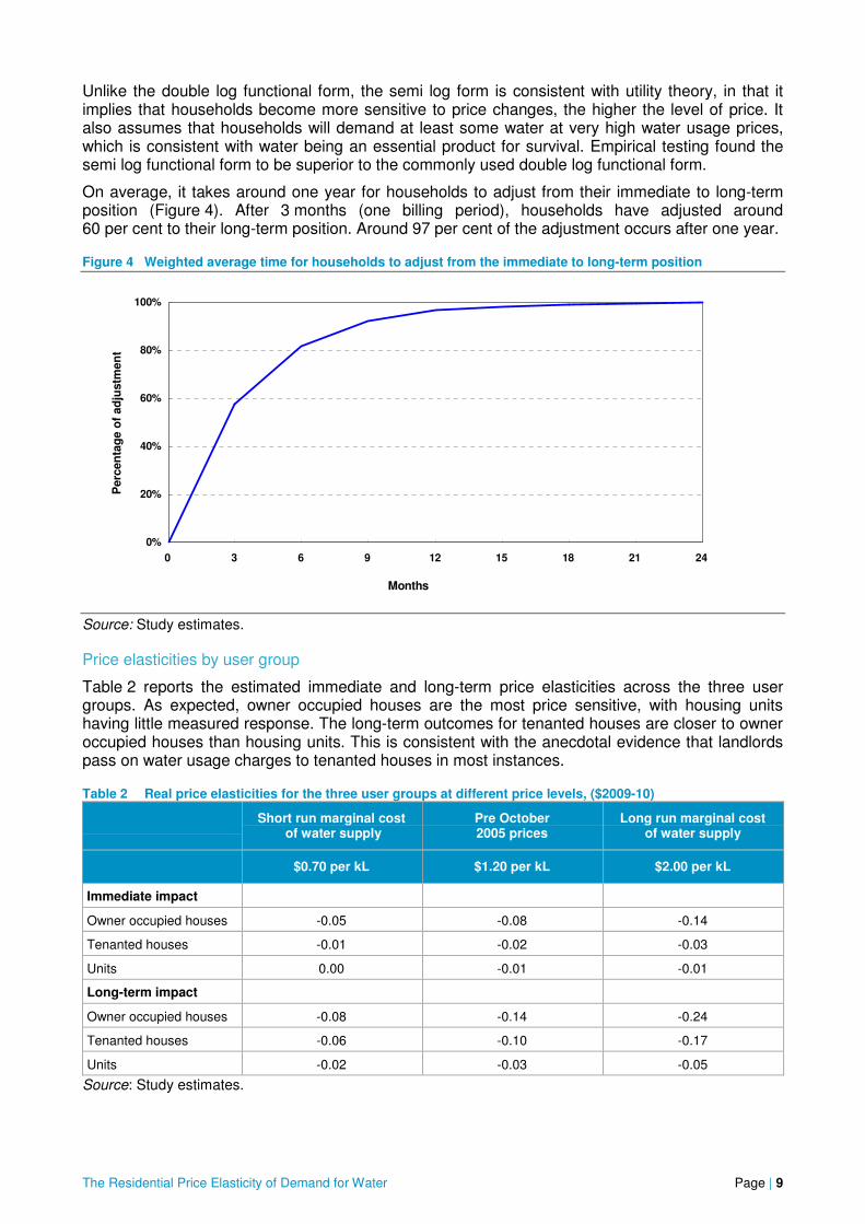
On average, it takes around one year for households to adjust from their immediate to long-term position (Figure 4). After 3 months (one billing period), households have adjusted around 60 per cent to their long-term position. Around 97 per cent of the adjustment occurs after one year.
Figure 4 Weighted average time for households to adjust from the immediate to long-term position
Source: Study estimates.
Price elasticities by user group
Table 2 reports the estimated immediate and long-term price elasticities across the three user groups. As expected, owner occupied houses are the most price sensitive, with housing units having little measured response. The long-term outcomes for tenanted houses are closer to owner occupied houses than housing units. This is consistent with the anecdotal evidence that landlords pass on water usage charges to tenanted houses in most instances.
Table 2 Real price elasticities for the three user groups at different price levels, ($2009-10)
Short run marginal cost of water supply
Pre October 2005 prices
Long run marginal cost of water supply
$0.70 per kL $1.20 per kL $2.00 per kL
Immediate impact
Owner occupied houses -0.05 -0.08 -0.14
Tenanted houses -0.01 -0.02 -0.03
Units 0.00 -0.01 -0.01
Long-term impact
Owner occupied houses -0.08 -0.14 -0.24
Tenanted houses -0.06 -0.10 -0.17
Units -0.02 -0.03 -0.05
Source: Study estimates.
0%
20%
40%
60%
80%
100%
0 3 6 9 12 15 18 21 24
Months
Perc
en
tag
e o
f ad
justm
en
t

The Residential Price Elasticity of Demand for Water Page | 10
The results demonstrate the importance of developing individual price elasticity estimates for different user groups. For Sydney, in 2007-08, around 75 per cent of residential property growth was housing units. This pattern of property growth will increase the proportion of households that are largely unresponsive to water usage prices. This will reduce the overall response of residential demand to changes in water usage prices, all other factors held constant.4
Price elasticities and participation in subsidised water efficiency programs
Subsidised water efficiency programs included in the study were WaterFix,5 DIY Kits6 and washing machine rebates.7 The estimated immediate impact of the programs is shown in Table 3. The impact of WaterFix and washing machine rebates is close to 10 per cent of a household’s total demand.
Table 3 Immediate impact of WaterFix, washing machine rebates and DIY kits on demand, per cent
Water efficiency program Immediate impact on household demand
WaterFix -9%
Washing machine rebate -7%
DIY kits -1%
Source: Study estimates.
An important finding of the study was that for households that did participate in a water efficiency program, their long-term elasticity is about half of those households that did not participate in a program (Table 4). Improvements in a household’s water appliance efficiency appear to both lower its average water demands and reduce its responsiveness to changes in water usage prices.
Table 4 Real price elasticities and subsidised water efficiency programs
Short run marginal cost
of water supply
Pre October 2005 prices
Long run marginal cost
of water supply
$0.70 per kL $1.20 per kL $2.00 per kL
Immediate impact
No water efficiency participation -0.04 -0.07 -0.11
Water efficiency participation -0.04 -0.07 -0.11
Long-term impact
No water efficiency participation -0.10 -0.16 -0.27
Water efficiency participation -0.06 -0.10 -0.16
Source: Study estimates.
This outcome is further highlighted in Figure 5, which shows the long-term demand curves for owner-occupied houses that did and did not participate in a water efficiency program. Each group’s average demand for water is now virtually identical at the current water usage price of around $2.00 per kL.
4 Sydney Water is examining the possibility of requiring all new multi-unit dwellings to install separate meters for each
unit. 5 Under the WaterFix program, for $22, a qualified plumber will install a new water efficient showerhead, tap flow
regulators, a toilet cistern flush arrestor for single flush toilets and repair minor leaks. The cost to Sydney Water of
providing the WaterFix service is around eight times the contribution sought. 6 DIY Kits are a low cost alternative to the full WaterFix service.
7 Rebates have also been provided for a range of rainwater tanks, based on tank size and the number of indoor
connections. Given the range of rebates offered, it was not possible to develop separate estimates for the range of
rebates offered. Properties that received a rainwater tank rebate were excluded from the analysis.

The Residential Price Elasticity of Demand for Water Page | 11
Figure 5 Long-term demand curves, owner occupied properties
Source: Study estimates.
Water efficiency programs provide for more water efficient household appliances. These are the items one would expect households to install in the long-term in response to permanent increases in water usage prices. As such, once a household has upgraded the water efficiency of its showerheads, washing machine and toilet(s), the scope for further permanent reductions in water use becomes far more limited given the current efficiency of water use appliances.
As households replace old showerheads, washing machines and toilets, the stock of water use appliances is gradually becoming more water efficient. In Sydney, this process is underpinned by the water efficiency requirements mandated for new and renovated properties. The implication is that future changes to water usage prices can be expected to have a diminished long-term impact.
Households may again reduce their water use in response to increases in water usage prices with further improvements in the water efficiency of available appliances. However, step changes in the water efficiency of appliances are not expected in the medium term. The benefits of further improvements in water appliance efficiency will also need to be assessed in the context of the minimum flows required for the efficient operation of the sewage system.
Long-term price elasticities and property size
For owner occupied houses that had not participated in a water efficiency program, a strong relationship between the long-term price elasticity and overall property size was found (Figure 6).
Figure 6 Long-term real price elasticity and property size, owner occupied houses
Source: Study estimates.
-0.7
-0.5
-0.3
-0.1
0.1
0 200 400 600 800 1000 1200 1400 1600 1800 2000
Property size (m 2)
Ela
sti
cit
y (
@$
1.2
0 p
er
kL
)
$0.00
$0.40
$0.80
$1.20
$1.60
$2.00
150 170 190 210 230 250 270 290 310
Demand (kL/household/year)
Pri
ce (
$ p
er
kL
)
No water efficiency participation Water efficiency participation

The Residential Price Elasticity of Demand for Water Page | 12
Up to a property size of around 1,300m2, the long-term elasticity increased steadily (becoming more negative) with property size. For households with a property size less than around 600m2, the long-term elasticity ranges from almost totally unresponsive to -0.15. Between 600m2 to 1,300m2, the elasticity increases from around -0.2 to -0.6. However, as property sizes become very large (ie approaching 2,000m2), the elasticity of demand reverts back to highly inelastic.
In Sydney, it is expected that new houses will generally be on smaller blocks of land. This will occur in both ‘greenfield’ areas and existing areas as large blocks of land are subdivided. This will increase the proportion of smaller property sizes, reducing the overall impact of water usage prices on demand.
Potential for further application
This is the first study in Australia to apply a dynamic panel data model specification, the semi log functional form and the GMM econometric estimation method to household level data. The study demonstrates the importance of grouping households by likely differences in demand characteristics. Grouping households by the way they pay water usage charges, participation in water efficiency programs, and property size, allowed for a far greater understanding of the impact of water usage prices on demand.
As this is the first modelling in Australia using household level data, there are still a number of important estimation issues to be further examined and potential improvements to be made. There is also more diversity in the level and structure of water prices across Australia compared to that analysed in this study.
Most water utilities in Australia should have the necessary household level data to undertake similar econometric analyses. Further studies using household level data, would provide policy makers, utilities and regulators with greater information on the most appropriate pricing strategies for their individual circumstances.

The Residential Price Elasticity of Demand for Water Page | 13
1 Introduction
Key messages
•••• There is currently strong interest in the potential for water usage prices to balance water supply and demand; however, the main gap in the scarcity pricing debate has been the absence of solid evidence on the price elasticity of demand for water.
•••• Sydney Water maintains detailed information on the water use of individual households. Sydney Water engaged Dr Vasilis Sarafidis, Lecturer in Econometrics, University of Sydney, to undertake a joint study applying econometric modelling to household level datasets.
1.1 The policy context
Interest in the use of prices to balance water supply and demand
Most Australian cities previously relied on rainfall fed dams to provide all or the majority of their water. Over the last decade, many Australian cities have experienced extended periods of low rainfall and reduced inflows to dams. The main initial response was mandatory restrictions on outdoor water use. In Sydney Water’s area of operations, drought restrictions were imposed for nearly six years (from October 2003 to June 2009). In June 2009, drought restrictions were replaced by Water Wise Rules: permanent water saving rules based on common sense approaches to using water efficiently (such as not watering gardens during the heat of the day). Generally, the use of drought restrictions has been part of a broader drought response, including significant investment in diversifying supply options and reducing demand through subsidised water efficiency programs.
It is in this context that a high level of interest has emerged among policy review agencies in using scarcity pricing to balance supply and demand for water. In its simplest form, scarcity pricing involves using water usage prices to reduce demand in times of scarcity. As sources of water supply diminish, water usage prices increase. As water sources are replenished, prices decrease. The potential for water usage prices to balance supply and demand is also part of the ongoing debate about the best way to price water, following the implementation of past reforms such as usage-based pricing and full cost recovery.
In 2008, the Productivity Commission released a discussion paper on urban water reform (PC 2008). The Commission noted that pricing regimes recovered operating costs and a return on investments, but did not reflect the scarcity of water in times of shortage. Instead, demand was managed through placing restrictions on households, which was assumed to have very significant costs for households. A key conclusion of the paper was that allowing a greater role for prices to signal water scarcity, and to allocate resources to augment supply, was an area that should be further investigated. A staff working paper published by the Productivity Commission in 2010 argued that scarcity pricing was preferable to imposing restrictions on water use, as restrictions prevented households from using water that they would have been willing to pay for (Barker et al 2010). The Commission is currently conducting a public inquiry into the urban water sector. One issue being examined is the scope for more efficient pricing, including scarcity pricing.8
In May 2010, Infrastructure Australia released a paper (prepared by PricewaterhouseCoopers) on urban water security (IA 2010). The paper included a recommendation to replace permanent water restrictions, described as a ‘second best’ mechanism to address unpriced supply/use externalities, with mechanisms that give customers choice in water security reliability.
The National Water Commission has supported further consideration of scarcity pricing in urban areas on the basis that it may be a more efficient way of balancing supply and demand and could significantly reduce the need for drought restrictions (NWC 2008).
8 Sydney Water’s submission to the Productivity Commission’s inquiry is available on the Commission’s website.

The Residential Price Elasticity of Demand for Water Page | 14
The Secretary to the Australian Treasury, Dr Ken Henry, has also called for the consideration of scarcity pricing as a measure to balance supply and demand (Henry 2008). He has argued that:
If we had a well functioning market in water, all users would pay a price that reflected not only the amortised costs of water storage and reticulation infrastructure, but also its scarcity value…In times of drought, water prices would rise in order to equate demand and supply; just how high they would rise depends not only upon the severity of the drought, but also the price-sensitivity of both market demand and market supply.
In a well functioning water market, drought-induced increases in the price of water would reallocate water among users, with a higher proportion of it flowing to those who valued it more highly. In any place, or at any time, at which its marginal value fell short of its price, water would not be used. On the other hand, if a suburban gardener valued her roses sufficiently highly, she wouldn’t have to stand by and watch them die.
…Instead, we have administered prices, legal protections on restraint of trade and, as a consequence, rationing. Rationing tends to be egalitarian. For example, in the towns and cities, the common practice is that ‘odds and evens’ water restrictions are first imposed, then progressively more restrictive, but persistently uniform, levels of access are mandated.
There is therefore no shortage of people and organisations interested in understanding the potential role of water usage prices in balancing the supply and demand for water.
Forecasting future water use and revenues
Water usage prices have been increasing in recent years in most capital cities to, in part, fund increases in operating and capital expenditure. In general, water usage prices have been increasing at a rate greater than inflation.
It is therefore important for water utilities to better understand the likely impact of these price increases on future levels of water use and associated revenues. With better information, the likely impact of changes to water usage prices can be incorporated into the price setting and planning process.
The price elasticity of demand
The effectiveness of water usage prices to balance supply and demand for water depends crucially on the price elasticity of demand. As noted by the Productivity Commission (2008):
The efficacy of allowing greater recourse to price to reduce the reliance on water restrictions depends on the responsiveness of demand for urban water to price. The responsiveness (elasticity) of demand determines the price increase necessary to achieve reductions in water consumption equivalent to those from water restrictions.
If demand is unresponsive to price, then the ability of water usage prices to reduce consumption during severe and sustained drought is limited. Alternatively, if demand is sufficiently responsive to price, then price increases could viably be used to replace or supplement drought restrictions. Equally important is how long it takes households to respond to changes in water usage prices. If households are slow to respond to price increases, larger increases will be necessary to quickly obtain the necessary reductions in water use during a severe and sustained drought.
In its Issues Paper for its inquiry into Urban Water, the Productivity Commission notes that some Australian studies estimate that the price elasticity of demand for water is in the range of -0.3 to -0.5, while some water utilities have suggested that demand is more inelastic than this (that is, closer to zero). There is limited evidence available on the time it takes households to react to changes in water usage prices.
In Sydney, the water usage price was around $1.00 per kL before the imposition of mandatory drought restrictions in October 2003. Table 1.1 shows the water usage prices necessary to reduce total demand by the same amount as drought restrictions for a range of different price elasticities.9
9 Sydney Water estimates that during Level 3 drought restrictions, the total demand for water was reduced by around
17 per cent compared to pre-restricted demand.

The Residential Price Elasticity of Demand for Water Page | 15
Table 1.1 Price increases necessary to reduce demand by 17 per cent (from $1.00 per kL)
Price elasticity Water usage price necessary to reduce demand by 17 per cent ($/kL)
-0.5 $1.34
-0.4 $1.43
-0.3 $1.57
-0.2 $1.85
-0.1 $2.70
-0.05 $4.40
Source: Sydney Water estimates.
The practicality and acceptability (to stakeholders and customers) of scarcity pricing is therefore highly dependent on the price elasticity of demand.
1.2 Sydney Water’s contribution
Sydney Water is Australia’s largest water utility, supplying water, wastewater, recycled water and some stormwater services to over four million people. This includes over 1.6 million residential households and 110,000 non-residential properties. Sydney Water’s area of operations extends south including the Illawarra, west including the Blue Mountains, north to the Hawkesbury River and east to the Tasman Sea (see map overleaf).
Sydney Water invests significant resources in maintaining detailed information on the water use of individual households.10 In forecasting demand and evaluating the effectiveness of subsidised water efficiency programs, Sydney Water has accumulated considerable information and data over the factors that have influenced demand. Initial work within Sydney Water demonstrated that these household level datasets were the best available to estimate the residential price elasticity of demand.
To provide policy makers with more reliable and transparent estimates of the price elasticity of demand, Sydney Water engaged Dr Vasilis Sarafidis, Lecturer in Econometrics, University of Sydney, to undertake a joint study applying econometric modelling to datasets developed by Sydney Water. By combining Sydney Water’s knowledge on the data issues involved in modelling water use with the skilled application of econometrics, this joint study has addressed many of the major challenges in estimating the price elasticity of demand of residential households.
1.3 Structure of this report
This section outlined the general interest in scarcity pricing, and the unique position of Sydney Water to support the development of reliable estimates of the price elasticity of demand for water.
Section 2 describes the residential consumption trends in Sydney Water’s area of operations, the timeframe for analysis and the three user groups chosen.
Section 3 describes the next level of detail in model development, namely, the explanatory variables, functional form, how the dataset was created, clustering of households, model specification and estimation technique.
Section 4 presents the results of the econometric models.
Supporting information on consumption trends, a discussion of previous studies for Sydney, and further detail on the econometric models are provided in appendices to the report.
10 Strictly defined, Sydney Water measures the water use of individual properties. By choosing a set of properties that
were not sold during the period of analysis, properties can be considered ‘households’.

The Residential Price Elasticity of Demand for Water Page | 16

The Residential Price Elasticity of Demand for Water Page | 17
2 High level issues
Key messages
•••• Houses and housing units have reduced their average water use over the past 10 years by about one quarter and 14 per cent, respectively. A number of factors have contributed to this sustained reduction in water use.
•••• There were no substantial increases in water usage prices until October 2005, well after drought restrictions were implemented. As such, the timeframe for the analysis is best kept to after October 2005, despite drought restrictions also being in force (Level 2 and Level 3).
•••• It is appropriate to have separate models for households in owner occupied houses, tenanted houses and housing units, because of the different ways they pay water usage charges.
Developing reliable estimates of the price elasticity of demand first requires an understanding of consumption trends and factors that have affected demand. Consumption trends and the identified factors affecting demand are described in Section 2.1. Section 2.2 covers the timeframe of analysis chosen for the study. Section 2.3 describes the different ways households pay water usage charges and the reason for modelling three separate user groups.
2.1 Consumption trends
Residential demand currently accounts for around two thirds of total water use. Of this, around 75 per cent is used by single residential dwellings (‘houses’), consisting of detached and semi-detached dwellings. Almost all houses have an individual water meter. Multi residential dwellings (‘housing units’) include units and flats, and account for the remaining 25 per cent of residential demand. Common meters, where one single meter serves an entire block of housing units, serve the majority of housing units.
Houses and housing units have reduced their average water use over the past 10 years by about one quarter and 14 per cent, respectively (Figure 2.1).
Figure 2.1 Average monthly demand (kilolitres), houses and housing units, July 2000 to June 2010
Source: Sydney Water.
10
15
20
25
30
Jul-0
0
Jan-0
1
Jul-0
1
Jan-0
2
Jul-0
2
Jan-0
3
Jul-0
3
Jan-0
4
Jul-0
4
Jan-0
5
Jul-0
5
Jan-0
6
Jul-0
6
Jan-0
7
Jul-0
7
Jan-0
8
Jul-0
8
Jan-0
9
Jul-0
9
Jan-1
0
Dem
an
d (
kL
/ho
useh
old
/mo
nth
)
Houses Housing units
Drought restrictions
in force
The Residential Price Elasticity of Demand for Water Page | 18
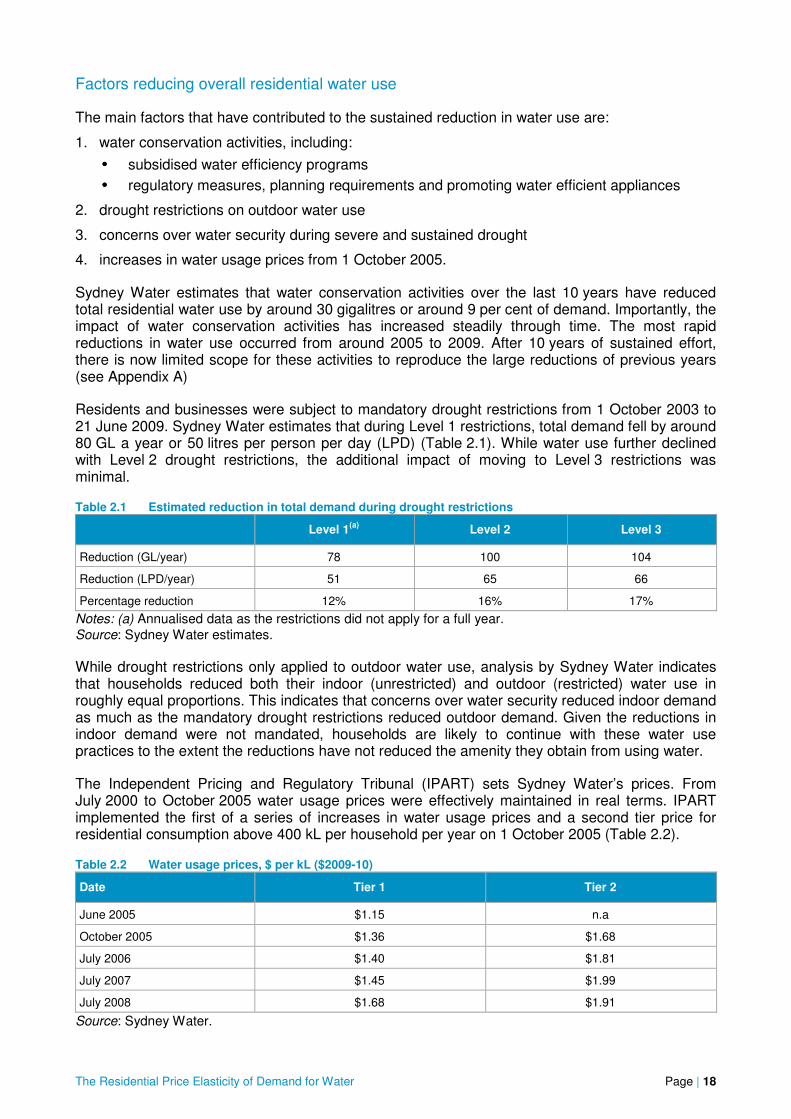
Factors reducing overall residential water use
The main factors that have contributed to the sustained reduction in water use are:
1. water conservation activities, including:
•••• subsidised water efficiency programs
•••• regulatory measures, planning requirements and promoting water efficient appliances
2. drought restrictions on outdoor water use
3. concerns over water security during severe and sustained drought
4. increases in water usage prices from 1 October 2005.
Sydney Water estimates that water conservation activities over the last 10 years have reduced total residential water use by around 30 gigalitres or around 9 per cent of demand. Importantly, the impact of water conservation activities has increased steadily through time. The most rapid reductions in water use occurred from around 2005 to 2009. After 10 years of sustained effort, there is now limited scope for these activities to reproduce the large reductions of previous years (see Appendix A)
Residents and businesses were subject to mandatory drought restrictions from 1 October 2003 to 21 June 2009. Sydney Water estimates that during Level 1 restrictions, total demand fell by around 80 GL a year or 50 litres per person per day (LPD) (Table 2.1). While water use further declined with Level 2 drought restrictions, the additional impact of moving to Level 3 restrictions was minimal.
Table 2.1 Estimated reduction in total demand during drought restrictions
Level 1(a)
Level 2 Level 3
Reduction (GL/year) 78 100 104
Reduction (LPD/year) 51 65 66
Percentage reduction 12% 16% 17%
Notes: (a) Annualised data as the restrictions did not apply for a full year. Source: Sydney Water estimates.
While drought restrictions only applied to outdoor water use, analysis by Sydney Water indicates that households reduced both their indoor (unrestricted) and outdoor (restricted) water use in roughly equal proportions. This indicates that concerns over water security reduced indoor demand as much as the mandatory drought restrictions reduced outdoor demand. Given the reductions in indoor demand were not mandated, households are likely to continue with these water use practices to the extent the reductions have not reduced the amenity they obtain from using water.
The Independent Pricing and Regulatory Tribunal (IPART) sets Sydney Water’s prices. From July 2000 to October 2005 water usage prices were effectively maintained in real terms. IPART implemented the first of a series of increases in water usage prices and a second tier price for residential consumption above 400 kL per household per year on 1 October 2005 (Table 2.2).
Table 2.2 Water usage prices, $ per kL ($2009-10)
Date Tier 1 Tier 2
June 2005 $1.15 n.a
October 2005 $1.36 $1.68
July 2006 $1.40 $1.81
July 2007 $1.45 $1.99
July 2008 $1.68 $1.91
Source: Sydney Water.
The Residential Price Elasticity of Demand for Water Page | 19
2.2 Timeframes for analysis
In Sydney, there were no substantial increases in water usage prices until October 2005. Drought restrictions were implemented well before this time, commencing with ‘voluntary’ measures in November 2002.
It was decided to limit the period of analysis for this study to when significant price increases occurred. As the shift from Level 2 to Level 3 drought restrictions appeared to have little further impact on total demand, the timeframe chosen for the analysis was the start of Level 2 drought restrictions in June 2004 to when drought restrictions were lifted in June 2009.
One issue with this timeframe is that the impact of the water usage price increases on demand could have been moderated because drought restrictions were in force. It could therefore be argued that the price elasticity of demand will be lower when drought restrictions are in force.
However, it is important to note that residential water use has changed little since drought restrictions were lifted in June 2009. Total demand increased by less than 3 per cent in 2009-10. This small increase is largely due to a hot and dry summer. This means that households have chosen to retain their indoor and outdoor water use practices established during drought restrictions.
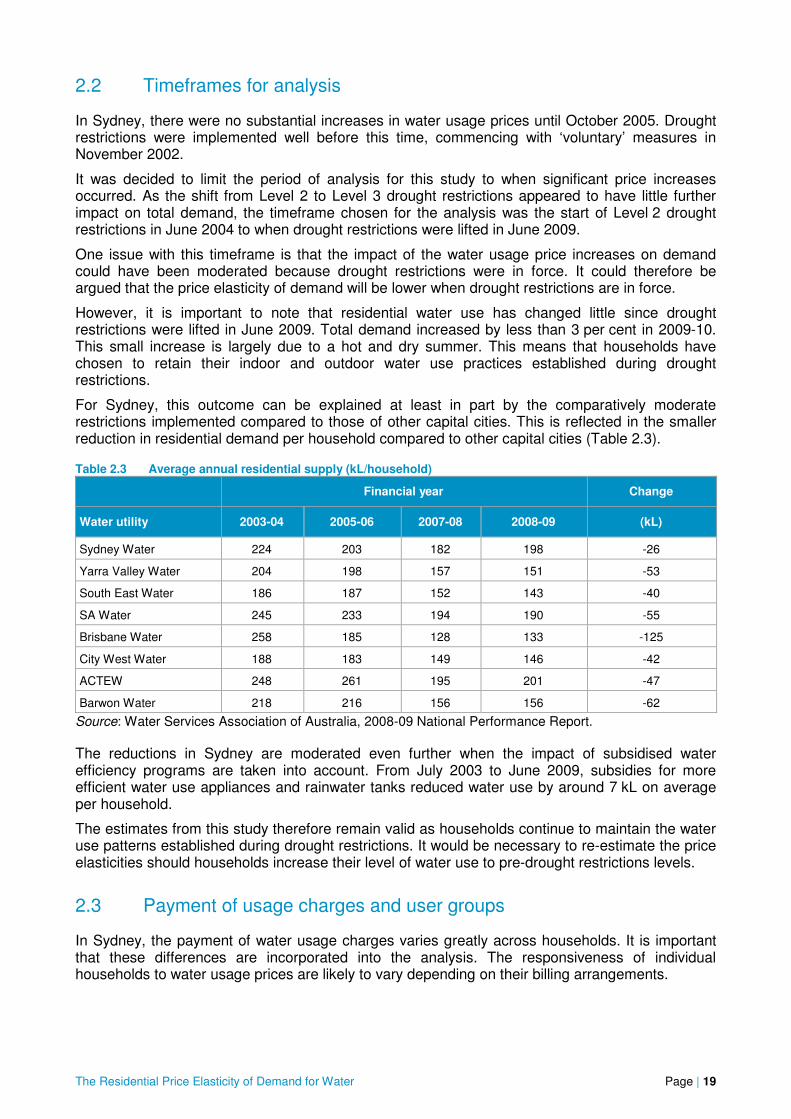
For Sydney, this outcome can be explained at least in part by the comparatively moderate restrictions implemented compared to those of other capital cities. This is reflected in the smaller reduction in residential demand per household compared to other capital cities (Table 2.3).
Table 2.3 Average annual residential supply (kL/household)
Financial year Change
Water utility 2003-04 2005-06 2007-08 2008-09 (kL)
Sydney Water 224 203 182 198 -26
Yarra Valley Water 204 198 157 151 -53
South East Water 186 187 152 143 -40
SA Water 245 233 194 190 -55
Brisbane Water 258 185 128 133 -125
City West Water 188 183 149 146 -42
ACTEW 248 261 195 201 -47
Barwon Water 218 216 156 156 -62
Source: Water Services Association of Australia, 2008-09 National Performance Report.
The reductions in Sydney are moderated even further when the impact of subsidised water efficiency programs are taken into account. From July 2003 to June 2009, subsidies for more efficient water use appliances and rainwater tanks reduced water use by around 7 kL on average per household.
The estimates from this study therefore remain valid as households continue to maintain the water use patterns established during drought restrictions. It would be necessary to re-estimate the price elasticities should households increase their level of water use to pre-drought restrictions levels.
2.3 Payment of usage charges and user groups
In Sydney, the payment of water usage charges varies greatly across households. It is important that these differences are incorporated into the analysis. The responsiveness of individual households to water usage prices are likely to vary depending on their billing arrangements.

The Residential Price Elasticity of Demand for Water Page | 20
Sydney Water’s billing arrangements can be summarised as:
•••• owners and landlords of houses are sent both service (fixed) and usage charges
•••• owners and landlords of housing units are sent service charges
•••• the strata corporation of housing units are sent water usage charges.
The households of owner occupied houses receive the strongest water usage price signal as they receive their water bills directly from Sydney Water. The bills contain information on prices as well as current and past levels of consumption.
For tenanted houses, a landlord can require the tenant(s) to pay the water usage charge if an individual meter serves the property. Anecdotal evidence suggests that most landlords pass on water usage charges to tenanted houses served by an individual water meter.
Sydney Water bills the strata corporation for the total water usage by the blocks of housing units served by common water meters. The tenant of a housing unit served by a common meter cannot be charged directly for water use. Instead, the costs must be recouped through rents. The strata corporation may recover an apportioned amount of water usage charges from owner occupied units through strata fees. However, no individual housing unit owner can directly control their allocated water usage charges. Any changes in water usage charges are averaged across all housing units.
These differences justify the separate analysis for the user groups of owner occupied houses, tenanted houses and housing units.11 It would be expected that owner occupied houses are the most responsive to water usage prices, while little response would be expected from housing units. The proportion of residential demand accounted for by each user group is shown in Figure 2.2.
Figure 2.2 Residential demand proportions, per cent, 2008-09 financial year consumption
Source: Sydney Water.
11 Around 5 per cent of residential demand is accounted for by townhouses and dual occupancies. These properties
were excluded from the analysis given difficulties in extracting individual billing arrangements.
Owner occupied houses
58% Tenanted houses 17%
Housing units 25%

The Residential Price Elasticity of Demand for Water Page | 21
3 Model specification and estimation technique
Key messages
•••• The explanatory variables tested in the econometric models were: water usage prices, the month and season, weather conditions, participation in water efficiency programs, income and disposable income, and previous levels of consumption.
•••• To allow the impact of the explanatory variables to vary across households within each user group, ‘clusters’ of properties were selected based on property size.
•••• The functional form chosen was semi log. This allows households to become more sensitive to water usage prices the higher the level of price while still ensuring households demand at least some water even at very high prices.
•••• A dynamic regression model was specified, consistent with the intuitive observation that households need time to adjust to changes in water usage prices and other explanatory variables.
•••• The estimation technique employed was the Generalised Method of Moments (GMM). GMM is best suited given the likely correlation between some of the explanatory variables and the error term.
This section describes the detailed elements of the econometric models, namely: the explanatory variables; the choice of functional form; how households were selected and the explanatory variables created; the clustering approach of households; the dynamic specification of the model; and the estimation method. The results of the econometric analysis are presented in the next section.
3.1 The explanatory variables
Commonly identified variables that explain a household’s level of water use are:
1. the number of people living in the house (household size)
2. property size (as a proxy for garden size)
3. pool ownership
4. the season
5. weather conditions
6. the imposition of drought restrictions
7. the efficiency of water use appliances and rainwater tanks
8. disposable income
9. the price of water
10. previous levels of consumption.
This extensive list can be made more manageable by categorising the variables according to how they influence demand. This is done in Figure 3.1 and described briefly below.

The Residential Price Elasticity of Demand for Water Page | 22
Figure 3.1 Summary of explanatory variables
Household size, property size and pools
Household size, property size and pool ownership are important variables in explaining differences in the level of consumption between households at a point in time. A five person household on a large block of land with a pool is likely to use far more water than a two person household on a small block of land.
However, the objective of this study is to measure the expected change in demand due to changes in water usage prices, rather than seek to explain differences in the level of consumption across households. Therefore, it is constructive to transform the model into ‘first differences’, ie the difference between the variable in one period and its preceding period. The advantage of this approach is that it allows the effect of all ‘time invariant’ variables, some of which are unobserved at the household level, to be removed from the analysis. As a result, one can obtain unbiased estimates of the price elasticity of demand, controlling for other factors that may influence water use, including time invariant unobserved factors.
To that end, a fixed number of households was included in the analysis, such that property size remains constant over time and thereby its direct effect is removed through first-differencing. Furthermore, the number of households that either installed or removed a pool is minimal. More careful analysis is required for household size, since some households could be expected to have changed in size over the period of analysis, which spans about five years.
One way to reduce the number and proportion of households that changed size is through the selection process. For example, properties that were sold during the period of analysis are likely to have new owners with a different household size and/or water use preferences. Accordingly, properties that were sold during the period of analysis were excluded from the sample (see Section 3.3).
Household size
Property size
Pool ownership
The season
Disposable income
Previous levels of consumption
Weather conditions
Drought restrictions
Water prices
Differences in the level of consumption between households
Variations in demand across months
Short-lived fluctuations in demand
Water appliance efficiency
Habit formation
Changes to the underlying level of demand

The Residential Price Elasticity of Demand for Water Page | 23
For housing units, a further issue to be addressed is the percentage of total housing units occupied through time. Increases or decreases in vacancy rates can alter the overall ‘household size’ for a given block of housing units. The method used to address this issue was to include an occupancy rate variable. Such data are available on a monthly basis, for three geographic areas across Sydney. As such, including this variable inherently involves a degree of measurement error for individual blocks of housing units, although this is taken into account in estimation.
The season and weather
The season and weather are related variables that explain changes to the level of demand over time. The season and weather drive short lived fluctuations in demand rather than underlying changes. A particularly rainy week is unlikely to cause people to permanently reduce the amount they water their garden.
Commonly identified weather variables are temperature, rainfall and evaporation. Households tend to use more water with higher temperatures and evaporation (when gardens dry out more quickly and people may take longer or more frequent showers). Rainfall reduces the demand for water as it reduces the need for garden watering. Two approaches tested to model the season and weather variables were:
1. seasonal variables (either the four seasons or monthly variables) and the deviation from the average value of temperature, rainfall and evaporation,
2. the average level of temperature, rainfall and evaporation.
Weather patterns also vary across Sydney. There is generally more rainfall with cooler conditions on the coast compared to many inland areas. Temperature and rainfall outcomes were obtained from the Bureau of Meteorology (BoM) for 13 weather stations across Sydney. Evaporation data were available from four weather stations: Prospect, Sydney Airport, Richmond and Riverview.
Figure 3.2 shows the location of the weather stations and the coverage across Sydney for different distances from each weather station. The light green ring represents 4 km from the weather station, increasing to 9 km for the red ring. Properties included in the analysis were allocated weather conditions based on its proximity to a weather station.
Figure 3.2 Location of the weather stations used in the study
Source: Sydney Water based on Bureau of Metrology information.
Katoomba
Bellambi
Terry Hills
Richmond
Penrith Lakes
Camden
Liverpool
Parramatta
Canterbury
Riverview
Sydney Obser.
Sydney Airport
Prospect
Katoomba
Bellambi
Terry Hills
Richmond
Penrith Lakes
Camden
Liverpool
Parramatta
Canterbury
Riverview
Sydney Obser.
Sydney Airport
Prospect

The Residential Price Elasticity of Demand for Water Page | 24
Changes to underlying demand
Drought restrictions, the water efficiency of appliances, disposable income and water usage prices can influence a household’s underlying level of demand. These variables also vary through time. They cannot therefore be assumed to be time invariant and removed from the analysis through first differencing.
Drought restrictions
Drought restrictions limit the time and way households undertake outdoor watering. The timeframe of analysis chosen is where Level 2 and Level 3 drought restrictions were in force (see Section 2.2). As the move from Level 2 to Level 3 did involve additional restrictions on outdoor water use, it was necessary to include a variable for the time when Level 2 drought restrictions were in place. Previous research by Sydney Water found that the additional impact of moving to Level 3 restrictions was minimal.
Efficiency of water use appliances and rainwater tanks
Properties can reduce their demand for water by installing more water efficient appliances or substitution through rainwater tanks.
Sydney Water has implemented one of the largest, heavily subsidised water efficiency programs in the world. The largest residential program has been WaterFix. Just under one third of houses in Sydney have participated in the WaterFix program. Under the WaterFiX program, for $22, a qualified plumber will install a new water efficient showerhead, tap flow regulators, a toilet cistern flush arrestor for single flush toilets and repair minor leaks. The cost to Sydney Water of providing the WaterFix service is around eight times the contribution sought.
As Sydney Water has heavily subsidised such activities, it is appropriate to include explanatory variables for these actions rather than assume they are the outcomes of increases in water usage prices. It is important to note that the majority of the participation in water efficiency programs occurred prior to the increases in water usage prices. Over 270,000 households had already participated in WaterFix before October 2005. The peak year was 2000-01, when more than 84,000 households participated. Between July 2005 and June 2009, the total number of additional participating households was around 120,000 or 30,000 per year.
It is also likely that many households installed a subsidised rainwater tank in response to restrictions on their ability to water their gardens, rather than to save money due to water usage price increases. The cost per kilolitre of water from a rainwater tank is usually calculated at in excess of $5.00 per kL, well above past and current water usage prices.
Rebates for rainwater tanks were offered at various amounts depending on the size of the tank and the number of indoor connections. For this study, households that received a rainwater tank rebate were excluded from the analysis. This simplified the modelling of water efficiency programs to those that offered one standard product. Further research could examine the price elasticity of households that have installed a rainwater tank.
Disposable income
Households could become less responsive to increases in water usage prices given rising incomes. It might also be that changes in disposable income influence water use behaviours. Households may become thriftier in using water and other essentials, such as electricity, in response to reductions in their disposable income.
The estimated income of each household was determined as at June 2006 based on Australian Bureau of Statistics (ABS) 2006 census data at a census collection district (CCD) level. This income was then scaled by the growth in income published by the ABS12 for different income groups in the years 2003-04 and 2006-07 across NSW.
12 ABS 6523.0 Household Income and Income Distribution, Australia

The Residential Price Elasticity of Demand for Water Page | 25
The estimate of disposable income for owner occupied houses was based on an estimate of the proportion of income needed to meet mortgage repayments. Another unavailable variable would be the proportion of income needed to meet other utility bills.
Both the income and disposable income variables are subject to measurement error at both the household level (due to CCD level data) and through time (only three measurements). This means an average result is applied when some households may have no mortgage while others are paying a large proportion of their income towards mortgage repayments. Some account of this measurement error is taken in the estimation technique (see Section 3.6).
Water prices
Potential price variables include water usage price(s), the service (fixed) price and the total water bill paid by the household. The argument for including either the service price and/or total water bill is that households react to changes in the total amount they pay when they receive their water bills, rather than focus on the water usage price or total water usage charges.
For most households on individual meters in Sydney, water bills are dominated by usage charges rather than service charges (Table 3.1). Also, the service component per quarter has also only varied by around $5 over the 5 years to 2008-09, while usage charges have increased by around $30. As such, water usage prices were used in the analysis rather than service prices and total water bills.
Table 3.1 Quarterly water bill for a household using 50 kL per quarter, nominal prices
Water bill components 2004-05 2005-06 2006-07 2007-08 2008-09
Usage charge $50.65 $60.00 $63.20 $66.95 $80.50
Service charge $19.41 $19.18 $16.10 $14.04 $19.00
Total bill $70.06 $79.80 $79.30 $80.99 $99.50
% usage 72% 75% 80% 83% 81%
Source: Sydney Water estimates based on prices set by the Independent Pricing and Regulatory Tribunal.
From October 2005 IPART introduced a two-tier water usage price structure for residential households served by an individual meter. The second tier applied to water use greater than 400 kL per year. Households served by common meters (ie housing units) were charged the tier 1 price only. IPART reverted back to a one-tier structure from July 2009.
In practice, the tiers were implemented based on the average daily consumption for each meter read period. The second tier price was applied to any consumption greater than 1.096 kL (400/365) of consumption per day within a meter read period. Around one quarter of houses paid the tier 2 water price on at least some of their water use during the period of analysis.
A two-tier tariff structure can create additional issues in estimating the price elasticity of demand. Some households are paying a different marginal (tier) price for water based on their level of water use. It also means that a weighted average price (total usage charges divided by total use) can vary from one period to the next due to both the level of consumption and changes in water usage prices.
The issues associated with tiered tariff structures are outlined in Taylor (1975), which surveys studies that sought to estimate the price elasticity of demand for electricity. Subsequent work by Nordin (1976) indicates that with a tiered tariff structure, the appropriate price variables to include are:
1. the marginal (highest) price paid for water by the household, and
2. the difference between the household’s total water bill and what they would have paid if all water consumption was charged at the marginal price.
These price variables were calculated in addition to a weighted average price paid per kL for each residential household.

The Residential Price Elasticity of Demand for Water Page | 26
300 Quantity (kL)
$5
$0
$10
150
Habit formation
A household’s water use preferences are likely to have a degree of persistence due to habit formation. Habit formation is the process by which a behaviour becomes habitual or an established custom. For example, the residents of a household may have the established custom of usually showering twice per day in hot weather conditions or watering the garden on certain days during the week.
Habit formation means that the response by a household to a change in water usage prices or other factors is likely to occur through time. This means it is necessary to analyse both the immediate and the long-term impact of changes in water usage prices.
In econometric modelling, habit formation can be addressed through the dynamic specification of the econometric models. This usually involves including previous periods of consumption in the econometric model (see Section 3.5).
3.2 Functional form
The functional form applied to water consumption and the explanatory variables determine the basic shape of the demand curve for water. The choice of functional form for water is still an open issue. The three main types of functional form are linear, double log and semi log. The functional forms are illustrated in Figure 3.3.
Figure 3.3 Illustrative examples of linear, double and semi log functional forms
Source: Sydney Water
As illustrated in Figure 3.3, the three key characteristics of each form are:
1. the maximum level of water use for each household with no water usage charge
2. whether price increases can eliminate all demand (existence of a ‘choke price’)
3. the elasticity of demand at different price levels.
The choice of functional form is important because each form implies a different response by households throughout the relevant price range. It is therefore necessary to consider which functional form is most likely to represent the demand for water by residential households.
Price ($/kL)
Linear
Double log
Semi log

The Residential Price Elasticity of Demand for Water Page | 27
Linear functional form
With a linear functional form, consumption and the explanatory variables are all expressed in levels or their observed amounts. The linear specification implies there is a maximum level of water a household would demand if water use were free (in the illustrative example, 300 kL per year). It also implies the existence of a ‘choke price’ at which no water would be demanded from households ($10 per kL).
The linear specification also assumes that the change in water use in response to a given absolute price change is the same at every level of price. In the illustrative example, each one dollar increase in price (ie $2 to $3 to $4 per kL) generates the same absolute reduction (30 kL) in demand at all price levels. This means households become more sensitive to prices the higher the level of price.
A linear specification does not fit well with the expectation about the nature of the demand for water by households. The main problem is that the specification assumes there is a price at which households would consume no water. This is clearly not going to occur in practice, as water is an essential product for survival. Many households have a limited ability to replace some or all of their basic water needs from alternative sources, such as rainwater tanks. As such, even at very high water usage prices, households could be expected to demand at least enough water to meet their basic needs. This means that the linear demand curve is likely to overstate the responsiveness to prices at high price levels.
Double log functional form
A double log specification expresses both consumption and the explanatory variables in a logarithmic form. The level of water use at a zero price is infinite. It also has no choke price, meaning households will always demand some amount of water even at very high water usage prices.
The double log specification assumes a constant elasticity of demand at all price levels. That is, at all price levels a given percentage change in price will result in the same percentage change in demand.
The double log specification is popular with researchers because it has the advantage that the estimates are easy to interpret. The coefficient for price(s) reflects the empirical elasticities. A paper by Howe and Linaweaver (1967, pg. 20) defend their selection of the double log specification by arguing that ‘theoretical considerations fail to specify a unique functional form’.
However, for the same reason that leads to ease of interpretation, this specification implies a lack of consistency with utility theory (see, for example Al-Quanibet and Johnston, 1985). In particular, it leads to a constant-elasticity form of water demand, according to which consumers are equally sensitive to changes in price regardless of the level of price. On this view households would significantly alter their water use in response to very small absolute changes (but large relative changes) in water usage prices at low price levels. Such outcomes are unlikely to occur in practice.
Semi log functional form
Under the semi log specification, consumption is expressed in logarithmic form while all explanatory variables are expressed in levels or their observed amounts. The semi log model assumes a maximum level of consumption at zero prices with no choke price.
The semi log model also assumes that households become more sensitive to price the higher the price. The elasticity is measured by multiplying the price coefficient(s) by the price level.
A price elasticity scaled to price without a choke price is likely to best match the actual response by households to changes in water usage prices. For these reasons, the semi log functional form was preferred for this study. The outcomes from the semi log functional form were also tested against the double log functional form using the approach developed by Davidson and MacKinnon (1981) for non-nested models. The semi log form was empirically supported by the data relative to the double log form.

The Residential Price Elasticity of Demand for Water Page | 28
3.3 Creating the dataset
For this study, ‘panel data’ analysis was employed, where the consumption of individual households through time is analysed. Some of the advantages in using panel data rather than the aggregate water use of each user group through time are described in Appendix C.
There were two main tasks in creating the dataset for analysis. The first was to select the households that were likely to have a stable household size during the period of the analysis.
The second was to create the explanatory variables. One issue with using household level data, is that the meter reads taken for all households in a particular quarter, can measure consumption over quite different periods of time. This means that it was necessary to align the explanatory variables with the meter reading periods of each household. Furthermore, ‘stratified’ sampling techniques were used to ensure the households included were representative of all households.
Household selection
The households included in the selection process were all those with a meter read between 1 January 2004 and 31 March 2004. Just over one million households met this criterion.
Households were then excluded based on several filters. Two key filters were whether the property was sold during the period of analysis and its participation in a water efficiency program other than WaterFix, DIY kits and washing machine rebates. For tenanted houses, households were removed if its level of consumption was 10 times greater or less than its average daily consumption in the corresponding quarter of the previous year.
To maintain the features of all households in the sample, a stratified sample was chosen. This was done by selecting the number of houses per CCD consistent with the proportion of houses to the total number of dwellings in that CCD. This meant that CCDs dominated by houses had more houses selected than those dominated by housing units.
Finally, households were excluded if their meter read periods were outside 80 to 110 days. This criterion promotes a degree of consistency across households in that their meters were read four times a year at roughly equal intervals.
Based on these selection processes, the total number of households included in the analysis were:
•••• Owner occupied houses: 70,277
•••• Tenanted houses: 24,427
•••• Blocks of housing units: 3,294 (around 10 individual housing units per block).
The timeframe of the analysis permitted 20 meter reading periods. The total number of observations in each sample is therefore very large. There are over 1.4 million observations for owner occupied houses.
Creating the explanatory variables
For each household included in the analysis, explanatory variables were created to match its meter read periods. In summary, this involved:
•••• creating daily weather conditions (rainfall, temperature and evaporation) then aggregating and averaging them for the weather station(s) assigned to each household
•••• determining the water usage price(s) paid by the household each period. If prices changed during a meter read period, the ‘average’ price was calculated based on the number of days the different prices applied
•••• creating variables for Level 2 drought restrictions, the season, months and participation in water efficiency programs based on the days within each meter read period
•••• estimating income and disposable income by CCD and allocating each household its value based on its CCD.
This process overcame the main challenge with household level data by creating explanatory variables that aligned with the time periods over which consumption is measured.

The Residential Price Elasticity of Demand for Water Page | 29
3.4 Clustering households by property size
It is plausible to expect that individual households within each user group respond differently to changes in the explanatory variables. For example, households that occupy a large property - and are likely to undertake more outdoor watering - are anticipated to be more sensitive to the season and weather conditions compared to households living on small blocks of land. Ignoring this effect and estimating instead a single model for the whole sample of a given user group is likely to result in biased estimates and invalid inferences (see for example, Sarafidis and Weber, 2010).
To address this issue, the households within each user group were clustered into sub groups based on the size of the household’s property, which is an observed variable. Separate models for each cluster were then estimated. The results reported are the weighted average estimates across clusters, with the weights determined by the number of households within each cluster.
Clustering analysis is a method used to determine the natural groupings of a sample of entities according to a prespecified range of observed characteristics. Therefore, observations grouped into the same cluster are deemed to be more similar than those assigned to different clusters according to a measure of similarity.
There are broadly two approaches to clustering; partitional methods and hierarchical methods. The former groups the entities into a fixed number of non-overlapping clusters, minimising some criterion function. The latter begins with each entity as a distinct cluster and subsequently builds a hierarchy of observations by merging the entities into successively larger clusters.
This study used the partitional clustering approach to obtain the optimal partition. Given a fixed number of clusters and some initial partition, the optimal partition of households into different clusters was determined by minimising the ‘squared-error’ criterion, which is the sum of squared deviations between each observation and the centroid (i.e. the mean value of property size) of a cluster in which a particular observation belongs. The initial partition was obtained using a hierarchical clustering solution. The optimal number of clusters is determined based on the Calinski-Harabasz criterion.
The interested reader may refer to Everitt (2003) and Wedel and Kamakura (1999) for a general treatment of clustering analysis. An application of the partitional clustering approach in panel data models can be found in Sarafidis (2006). Clustering analysis based on unobserved characteristics has been studied, among others, by Sarafidis and Weber (2010).
3.5 Dynamic specification
It is natural to expect that households, on average, react over time to changes in water usage prices. In the first instance, households can receive their water bills based on the new prices up to three months after the price change occurred. In the immediate period, households can alter their demand given their existing stock of water use appliances. Over time, households may decide to buy more water efficient appliances or choose different types of plants that require less watering.
A popular way of accounting for the fact that households take time to adjust fully to changes in water usage prices is to specify an autoregressive, distributed lag (ARDL) model. In the present context this involves including lagged values of the dependent variable (consumption), which captures habit formation and the cost of adjustment, together with lagged values of water usage prices to capture short run fluctuations in demand. The benefits of an ARDL model are that it provides information on the immediate and long-term response by households to changes in water usage prices and the time taken to adjust from their immediate to long-term position. An ARDL model therefore is well suited to providing policy makers with the relevant information over the potential for using water usage prices to balance the supply and demand for water.

The Residential Price Elasticity of Demand for Water Page | 30
3.6 Estimation method
The most widely used estimation method in econometrics is Ordinary Least Squares (OLS). OLS estimates the coefficient values (the impact) of the explanatory variables by minimising the ‘sum of squared differences’ between actual and predicted values.
A key assumption of this method is that all explanatory variables are ‘exogenous’ – in other words, they are determined outside the model under investigation. A direct implication of this is that the explanatory variables are uncorrelated with the unobserved error term. The latter reflects everything the model does not control for, including random noise. When this assumption is violated for a given explanatory variable, the variable is called ‘endogenous’. There are a number of issues with modelling the demand for water, which imply that the explanatory variables cannot be considered to be determined exogenously.
In particular, one issue is that with a two-tier structure of water usage prices, the price paid by each household is dependent on its level of consumption. This means an increase in water use can actually cause an increase in the marginal and average usage price paid if the household’s water use exceeds the threshold for the second price tier. This situation creates a simultaneous cause-and-effect relationship between consumption and water usage prices, which violates the exogeneity assumption for the price of water.
Furthermore, the previous level of consumption, which is used as an explanatory variable in the model, is by construction correlated with time-invariant sources of unobserved heterogeneity, like household size, captured by the error term, and therefore is not exogenous either.
Violation of the exogeneity assumption means that OLS-based estimation techniques are likely to result in biased (wrong) estimates of the coefficient values of the explanatory variables. Furthermore, these estimates can fail to converge to the true values even in very large samples. Inferences over the statistical significance are also invalidated in this case.
An alternative estimation technique is the method of Maximum Likelihood (ML). ML selects values of the model parameters that produce the distribution most likely to have resulted in the observed data. ML requires a complete specification of the model and its probability distribution. However, in panel data models with a relatively small number of observations through time (around 20 for this study), the distribution of the ML estimator can be sensitive to what is assumed about the distribution of the initial observations, for which there is no a priori information in this case.
To address the identified issues with the panel dataset, this study employed the Generalised Method of Moments (GMM) estimation method. GMM is a very general estimation method, which, similar to other estimation procedures, is based on the minimisation (or maximisation) of a criterion function. The difference lies in the type of the criterion function used and its specification requirements.
To obtain some intuitive insight for GMM, suppose the equation of interest is given by:
,iii uXy += β
and the explanatory variable, Xi, is endogenous, such that E(Xiui) ≠ 0. This implies that Xi is correlated with ui.
Suppose now there exists variables, Zi, which are correlated with Xi but not with ui. This can be expressed as a set of ‘moment conditions’: E(Ziui) = 0. Notice that these moment conditions are theoretical and therefore unobserved. However, matching these moments with their sample counterparts yields
( ) .1∑=
i
iiuXN
g β
Therefore, the objective behind GMM is to choose estimates of β so that the observed sample moments, ie the elements of g(β), are as close to the theoretical moments, which equal zero, as possible. Hence, the method chooses the value of β that minimises

The Residential Price Elasticity of Demand for Water Page | 31
( ) ( ) ( ),ˆ'ˆˆGMMGMMGMM WgNgJ βββ =
that is, a quadratic distance between ( )GMMg β̂ and zero. W is a weighting matrix that accounts for
possible correlations among the sample moment conditions when the errors are serially correlated and heteroskedastic.
The GMM estimation procedure employed in this study takes place in two steps. In the first step, a ‘consistent’ estimator is obtained by setting W equal to an identity matrix. In the second step an
estimate of W, obtained from the first-step results, is used in the criterion function, ( )GMMJ β̂ .
Therefore, the second-step estimates are efficient under serial correlation and heteroskedasticity in the error process.
For a general treatment of GMM, the interested reader may refer to Mátyás (1999) and Hall (2005).

The Residential Price Elasticity of Demand for Water Page | 32
4 The results
Key messages
•••• At a water usage price of $1.20 per kL (in 2009-10 dollars), the estimated immediate and long-term real price elasticities for the demand for water are:
Household type Immediate Long-term
Owner occupied houses -0.08 -0.14
Tenanted houses -0.02 -0.10
Housing units -0.01 -0.03
Weighted average -0.05 -0.11
•••• On average, it takes around one year (4 billing periods) for households to adjust from their immediate to long-term position.
•••• It was found that once a household had upgraded the efficiency of its water use appliances (eg. a four star washing machine), its long-term price elasticity is almost halved. Improvements in a household’s water appliance efficiency appear to both lower its average water demands and reduce its responsiveness to changes in water usage prices.
•••• For Sydney, the combination of a forecast increase in the proportion of housing units, new houses with smaller property sizes, and improvements in water appliance efficiency, will reduce the ability of water usage prices to influence residential demand levels.
This section presents the outcomes of the econometric modelling, focussing on the immediate and long-term impact of changes in water usage prices. Appendix E contains detail on the outputs from the models, including model diagnostics.
Section 4.1 briefly summarises the user groups, explanatory variables and elasticity price range. Sections 4.2 to 4.4 then present the outcomes for owner occupied houses, tenanted houses and housing units. Weighted average results are presented in section 4.5.
4.1 User groups, variables and the elasticity price range
As described previously, the three broad user groups chosen for analysis were owner occupied houses, tenanted houses and housing units. For owner occupied and tenanted houses, households were first grouped by those that did and did not participate in a water efficiency program. Clusters of households based on property size were then determined for each of the four sub groups. There were 49 clusters in total for owner occupied houses and 14 for tenanted houses (Table 4.1). Together with housing units (as a single model), 64 econometric models were estimated from the available households.
Table 4.1 User groups and clusters
Date No. of households No. of clusters
Owner occupied houses 70,227 49
No water efficiency program participation 32,446 18
Water efficiency program participation 37,781 31
Tenanted houses 24,427 14
No water efficiency program participation 19,276 7
Water efficiency program participation 5,151 7
Housing units (blocks) 3,294 1
TOTAL 97,948 64
Source: Study estimates.

The Residential Price Elasticity of Demand for Water Page | 33
To calculate the average outcome for owner occupied and tenanted houses, individual outcomes were weighted by the number of households in each cluster. The weighted average results for all residential properties were based on the proportion of total demand for each user group.
Consumption and the explanatory variables
Consumption was measured as the average daily demand for the household within each meter read period. This approach avoided the need to account for changes in consumption from each meter read period to the next due to differences in the number of days between meter read periods.
The explanatory variables included in the final econometric models developed for owner occupied and tenanted houses were:
•••• the weighted average water usage price paid in the meter read period
•••• the weighted average water usage price paid in the previous five meter read periods
•••• average daily consumption in the previous meter read period
•••• deviations from the average for rainfall and evaporation
•••• the months covered by each meter read period
•••• the proportion of time spent in Level 2 drought restrictions for the meter read period
•••• the timing of participation in the WaterFix, DIY Kits and washing machine rebate water efficiency programs.
For housing units, the levels of temperature and rainfall were used instead of the deviations from the average together with monthly variables. This approach was taken due to difficulties in creating the monthly variables rather than the preferred set of explanatory variables.
Box 4.1 provides some further description of how the various explanatory variables identified in section 3.1 performed in the econometric models.
Box 4.1 Development of the econometric models
Season and weather
The most plausible results were achieved using a combination of monthly variables with the deviations from the average for rainfall and evaporation. The monthly variables could then be aggregated into the seasons of summer, autumn, winter and spring. With evaporation included in the model, temperature was generally found to be statistically insignificant and often with a negative coefficient value.
Immediate and long-term price effects
Up to five lags of water usage prices were tested in the models together with a lag of consumption. The fifth lag of water usage prices was generally found to be statistically insignificant. It is worth mentioning that the long-term price elasticity estimate remained largely unchanged even if further lags of price were removed.
Including the marginal price and the difference between the total bill and what the consumer would have paid if all water use was charged at the marginal price (as recommended by Nordin (1976)), did not prove worthwhile compared to using the weighted average water usage price. This could reflect the fact that the second tier of prices only applied for relatively high level of water use. As such, the price only applied to around one quarter of households at some period, and often only on a small amount of water use.

The Residential Price Elasticity of Demand for Water Page | 34
Box 4.1 cont. Development of the econometric models and explanatory variables
Other factors that could influence underlying demand
Income and disposable income were not statistically significant in the models. This may be interpreted as saying that those households that did not move property during the period of analysis did not appear to alter their water use in response to changes in their income or disposable income. However, a significant income rise might mean a household upgrades to a larger house and/or property size and perhaps increase their water use. This possibility was not tested in the econometric models.
In addition, the income and disposable income variables were subject to some measurement error as they were not available at a household level. Although measurement error was allowed for in estimation by using lagged values of disposable income as instruments, it could be the case that statistically significant relationships could be established with more disaggregated (accurate) data.
Aggregate and cluster models
Aggregate models for owner occupied and tenanted households that did and did not participate in a water efficiency program were first formulated and tested. While the models generated plausible coefficient values, the model diagnostics were often poor. This indicated a level of bias on the coefficient estimates, which is anticipated since the regressors are not exogenous and aggregate models assume that all parameters are homogeneous (equal) across all households.
Clustering households by property size resolved the identified problems for most clusters, with greatly improved model diagnostics. In terms of coefficient estimates, the significant changes were in the season and weather variables, rather than water usage prices. This suggests that the problems with the aggregated models were primarily modelling the effects of the season and weather at a household level.
Elasticity price range
The immediate and long-term real price elasticity estimates are reported for three different price levels in 2008-09 dollars. The lowest is $0.70 per kL, broadly equal to the short run marginal cost of providing potable water from dams. This is the level of prices that could be charged under a scarcity pricing model when dam storage levels are high. The highest is $2.00 per kL, broadly equal to the long run marginal cost of augmenting supply in Sydney (ie increasing the capacity of the desalination plant). The middle amount is $1.20 per kL, broadly equal to the water usage price prior to the implementation of the price increases from October 2005.
4.2 Owner occupied houses
In 2008-09 there were around 800,000 owner occupied houses, representing around 60 per cent of total residential demand. Of these, around 250,000 households (some 30 per cent) had participated in a subsidised water efficiency program (WaterFix, washing machine rebate or DIY Kit).
No participation in a subsidised water efficiency program
The average daily demand of households and real water usage prices (in 2009-10 dollars) over the five years to June 2009 is shown in Figure 4.1. Comparing the first four quarters of data to the last four, the average demand for water fell by just over 8 per cent. Over the same time, average real water usage prices increased by over 40 per cent.

The Residential Price Elasticity of Demand for Water Page | 35
Figure 4.1 Demand and real prices, owner occupied houses, no water efficiency program participation
Source: Sydney Water.
The immediate and long-term real price elasticity estimates are shown in Table 4.2. The immediate real price elasticity of demand ranges from -0.06 to -0.16. The long-term real price elasticity of demand ranges from -0.10 to -0.30.
Table 4.2 Real price elasticities, owner occupied houses, no participation in water efficiency programs
Short run marginal cost of water supply
Pre October 2005 prices
Long run marginal cost of water supply
$0.70 per kL $1.20 per kL $2.00 per kL
Immediate impact -0.06 -0.10 -0.16
Long-term impact -0.12 -0.20 -0.33
Source: Study estimates.
The estimated rate of adjustment is shown in Figure 4.2. On average, households adjusted around half of the way to their long-term position after three months. Around 95 per cent of the adjustment occurred after one year.
Figure 4.2 Path of adjustment, owner occupied houses, no water efficiency program participation
Source: Study estimates.
0.0
0.1
0.2
0.3
0.4
0.5
0.6
0.7
0.8
Mar
-04
Jun-0
4
Sep-0
4
Dec
-04
Mar
-05
Jun-0
5
Sep-0
5
Dec
-05
Mar
-06
Jun-0
6
Sep-0
6
Dec
-06
Mar
-07
Jun-0
7
Sep-0
7
Dec
-07
Mar
-08
Jun-0
8
Sep-0
8
Dec
-08
Mar
-09
Jun-0
9
Dem
an
d (
kL
/ho
useh
old
/day)
$1.00
$1.10
$1.20
$1.30
$1.40
$1.50
$1.60
$1.70
Real
pri
ce (
$ p
er
kL
)
Demand Real price
0%
20%
40%
60%
80%
100%
0 3 6 9 12 15 18 21 24
Months
Perc
en
tag
e o
f ad
justm
en
t

The Residential Price Elasticity of Demand for Water Page | 36
The estimated immediate and long-term demand curves are shown in Figure 4.3. The average demand for water for these households was around 222 kL per year in 2008-09 when the average water usage price was around $1.65 kL. If the water usage price is increased by around 20 per cent to $2.00 per kL, the immediate reduction in demand is around 6 kL per year. The long-term expected reduction is 12 kL per year.
Figure 4.3 Immediate & long term demand curves, owner occupied, no water efficiency program participation
Source: Study estimates.
For owner occupied houses that had not participated in a water efficiency program, a strong relationship between the long-term price elasticity and property size was found (Figure 4.4). Up to a property size of around 1,300m2, the long-term elasticity increased steadily (becoming more negative) with property size. For households with a property size less than around 600m2, the long-term elasticity ranges from almost totally unresponsive to -0.15. Between 600m2 to 1,300m2, the elasticity increases from around -0.2 to -0.6. However, as property sizes become very large (ie approach 2,000m2), the elasticity of demand reverts back to highly inelastic.
Figure 4.4 Real price elasticity and property size, owner occupied houses, no water efficiency participation
Source: Study estimates.
$0.00
$0.40
$0.80
$1.20
$1.60
$2.00
150 170 190 210 230 250 270 290 310
Demand (kL/household/year)
Re
al
pri
ce
($
pe
r k
L)
Immediate Long-term
-0.7
-0.5
-0.3
-0.1
0.1
0 200 400 600 800 1000 1200 1400 1600 1800 2000
Property size (m 2)
Ela
sti
cit
y (
@$
1.2
0 p
er
kL
)

The Residential Price Elasticity of Demand for Water Page | 37
Participation in subsidised water efficiency programs
The average daily demand of households and real water usage prices over the five years to June 2009 is shown in Figure 4.5. It is important to note that many of the households included participated in a water efficiency program prior to the start of the analysis period. This means the reductions in their water use through improvements in appliance efficiency have already occurred before the increases in water usage prices from October 2005. For households that purchased a new water efficient washing machine during the period of analysis, their average demand fell by around 15 per cent over the 5 years to June 2009.
Figure 4.5 Demand and real prices, owner occupied houses, water efficiency program participation
Source: Sydney Water.
The immediate and long-term real price elasticity estimates are shown in Table 4.3. The immediate real price elasticity of demand ranges from -0.04 to -0.12. The long-term real price elasticity of demand ranges from -0.06 to -0.16. On average, households adjusted 57 per cent of the way to their long-term position after three months, with around 97 per cent adjustment after one year.
Table 4.3 Real price elasticities, owner occupied houses, participation in water efficiency programs, ($09-10)
Short run marginal cost of water supply
Pre October 2005 prices
Long run marginal cost of water supply
$0.70 per kL $1.20 per kL $2.00 per kL
Immediate impact -0.04 -0.07 -0.12
Long-term impact -0.06 -0.10 -0.16
Source: Study estimates.
The estimated impact of different water efficiency programs on household demand is shown in Table 4.4. The results indicate that WaterFix and a new water efficient washing machine can on average reduce a household’s water use by almost 10 per cent.
Table 4.4 Impact of WaterFix, washing machine rebates and DIY kits on demand (per cent)
Water efficiency program Immediate impact on household demand
WaterFix -9%
Washing machine rebate -7%
DIY kits -1%
Source: Study estimates.
0.00
0.10
0.20
0.30
0.40
0.50
0.60
0.70
0.80
Mar
-04
Jun-0
4
Sep-0
4
Dec
-04
Mar
-05
Jun-0
5
Sep-0
5
Dec
-05
Mar
-06
Jun-0
6
Sep-0
6
Dec
-06
Mar
-07
Jun-0
7
Sep-0
7
Dec
-07
Mar
-08
Jun-0
8
Sep-0
8
Dec
-08
Mar
-09
Jun-0
9
De
ma
nd
(k
L/h
ou
se
ho
ld/d
ay
)
$1.00
$1.10
$1.20
$1.30
$1.40
$1.50
$1.60
$1.70
Re
al
pri
ce
($
pe
r k
L)
WaterFix Washing machine rebate Water use price

The Residential Price Elasticity of Demand for Water Page | 38
These results indicate that improvements in a household’s water appliance efficiency appear to both lower its average water demands and reduce its responsiveness to changes in water usage prices. This outcome is to be expected as water efficiency programs provide for more water efficient household appliances. These are the items it would be expected households install in the long-term in response to permanent increases in water usage prices. As such, once a household has upgraded the water efficiency of its showerheads, washing machine and toilet(s), the scope for further permanent reductions in water use become far more limited given the current efficiency of water use appliances.
This outcome is further highlighted in Figure 4.6, which shows the long-term demand curve for owner-occupied houses that did and did not participate in a water efficiency program. Each group’s average demand for water is now virtually identical at the current water usage price of around $2.00 per kL.
Figure 4.6 Long-term demand curves, owner occupied properties
Source: Study estimates.
It is likely many households improved the efficiency of their water use appliances outside the programs offered by Sydney Water. On this basis, it could be expected that the future demand curve for all houses is closer to that of those that did participate in a water efficiency program.
4.3 Tenanted houses
In 2008-09 there were around 230,000 tenanted houses, representing around 17 per cent of total residential demand. Of these, just over 75,000 or around one third, had participated in a water efficiency program. The average daily consumption of properties that did and did not participate in a water efficiency program is shown in Figure 4.7.
The immediate and long-term real price elasticity estimates are shown in Table 4.6. The elasticities are generally lower than for owner occupied houses. They also have the same feature as owner occupied houses where the long-term elasticity for households that participated in a water efficiency program are lower compared to those households that did not participate.
The long-term demand curves for water are shown in Figure 4.8.
$0.00
$0.40
$0.80
$1.20
$1.60
$2.00
150 170 190 210 230 250 270 290 310
Demand (kL/household/year)
Pri
ce (
$ p
er
kL
)
No water efficiency participation Water efficiency participation

The Residential Price Elasticity of Demand for Water Page | 39
Figure 4.7 Average daily demand of tenanted houses, kL
Source: Sydney Water.
Table 4.6 Real price elasticity estimates at different price levels, tenanted houses, ($2009-10)
Short run marginal cost of water supply
Pre October 2005 prices
Long run marginal cost of water supply
Price elasticity $0.70 per kL $1.20 per kL $2.00 per kL
No water efficiency program
Immediate impact -0.01 -0.02 -0.03
Long-term impact -0.06 -0.11 -0.18
Water efficiency program
Immediate impact -0.01 -0.03 -0.04
Long-term impact -0.05 -0.08 -0.14
Source: Study estimates.
Figure 4.8 Long-term demand curves, tenanted houses
Source: Study estimates.
0.50
0.55
0.60
0.65
Mar
-04
Jun-0
4
Sep-0
4
Dec
-04
Mar
-05
Jun-0
5
Sep-0
5
Dec
-05
Mar
-06
Jun-0
6
Sep-0
6
Dec
-06
Mar
-07
Jun-0
7
Sep-0
7
Dec
-07
Mar
-08
Jun-0
8
Sep-0
8
Dec
-08
Mar
-09
Jun-0
9
Dem
an
d (
kL
/ho
useh
old
/day)
No WE participation WaterFix WMR
$0.00
$0.40
$0.80
$1.20
$1.60
$2.00
190 200 210 220 230 240 250 260 270
Demand (kL/property per year)
Real
pri
ce (
$ p
er
kL
)
No water efficiency participation Water efficiency participation

The Residential Price Elasticity of Demand for Water Page | 40
4.4 Housing units
In 2008-09 there were around 480,000 units, representing around 24 per cent of total residential demand. Of these, around 12 per cent had participated in a water efficiency program.
The average daily consumption of housing units (per block of units served by a common meter) and real water usage prices are shown in Figure 4.9. There is little difference in the average consumption of housing units between the first and last year of the analysis period.
Figure 4.9 Demand and real prices, housing units
Source: Sydney Water.
The immediate and long-term real price elasticity estimates are shown in Table 4.7. The estimated real elasticities are very small, consistent with the minimal effective water usage price signal received by households living in housing units.
Table 4.7 Real price elasticity estimates at different price levels, housing units, ($2009-10)
Level of prices ($/kL)
Price elasticity $0.70 per kL $1.20 per kL $2.00 per kL
Immediate impact 0.00 -0.01 -0.01
Long-term impact -0.02 -0.03 -0.05
Source: Study estimates.
3.90
4.00
4.10
4.20
4.30
4.40
4.50
4.60
4.70
Mar
-04
Jun-0
4
Sep-0
4
Dec
-04
Mar
-05
Jun-0
5
Sep-0
5
Dec
-05
Mar
-06
Jun-0
6
Sep-0
6
Dec
-06
Mar
-07
Jun-0
7
Sep-0
7
Dec
-07
Mar
-08
Jun-0
8
Sep-0
8
Dec
-08
Mar
-09
Jun-0
9
De
ma
nd
(k
L/b
loc
k/d
ay
)
1.00
1.10
1.20
1.30
1.40
1.50
1.60
1.70
Re
al p
ric
e (
$ p
er
kL
)
Demand Real price

The Residential Price Elasticity of Demand for Water Page | 41
4.5 Weighted average outcomes for residential households
The weighted average immediate and long-term real price elasticity estimates are shown in Table 4.8. The weighted average immediate real price elasticity ranges from -0.03 to -0.09. The long-term real price elasticity ranges from -0.06 to -0.18.
Table4.8 Weighted average real price elasticities, all residential households, ($2009-10)
Short run marginal cost of water supply
Pre October 2005 prices
Long run marginal cost of water supply
$0.70 per kL $1.20 per kL $2.00 per kL
Immediate impact -0.03 -0.05 -0.09
Long-term impact -0.06 -0.11 -0.18
Source: Study estimates.
The immediate and long-term real price elasticities are generally lower than previous studies in Australia, and well below the commonly assumed constant elasticity of -0.3. One reason for the difference is that this study analysed individual households across time. This allows for more accurate control of the other factors that affect demand. Other studies generally use bulk water data, which are affected by leak management programs, recycling, water efficiency programs and structural changes in water use by industrial and business users. For Sydney, in the current environment, bulk water demand does not provide an appropriate basis to estimate the price elasticity of demand.
The sensitivity of demand to the assumed elasticity of demand and functional form is highlighted in Figure 4.10. Figure 4.10 shows the long-term demand curve from the study estimates (based on the semi log form) and a demand curve based on the commonly employed ‘double log’ (constant elasticity) form with a price elasticity of -0.3. The curves are based on 2008-09 average consumption levels (around 202 kL per household per year) when average water usage prices were around $1.65 per kL.
One key difference between the study estimates and the double log functional form is the level of consumption at low water usage prices. Based on the double log functional form, demand increases by around 60 kL per household per year if the water usage price is reduced from $1.65 per kL to $0.70 per kL. As such, there is a substantial amount of assumed demand than can be reduced through modest price increases at low price levels.
Figure 4.10 Study estimates (long-term) and double log demand curves
Source: Study estimates.
$0.00
$0.40
$0.80
$1.20
$1.60
$2.00
150 170 190 210 230 250 270 290
Demand (kL/household/year)
Pri
ce (
$ p
er
kL
)
Long-term Double log @-0.3

The Residential Price Elasticity of Demand for Water Page | 42
Unlike the double log functional form, the semi log form is consistent with utility theory in that it implies that households become more sensitive to price changes the higher the level of price. It also assumes that households will demand at least some water at very high water usage prices, which is consistent with water being an essential product for survival. Empirical testing found the semi log functional form to be superior to the commonly used double log functional form.
On average, it takes around one year for households to adjust from their immediate to long-term position (Figure 4.11). After 3 months (one billing period), households have adjusted around 60 per cent of the way to their long-term position. Around 97 per cent of the adjustment occurs after one year. If it is necessary to reduce demand quickly (eg 6 months), relatively larger price increases will therefore be required given the rate at which households react to price changes.
Figure 4.11 Weighted average time taken to adjust from the immediate to long-term position
Source: Study estimates.
0%
20%
40%
60%
80%
100%
0 3 6 9 12 15 18 21 24
Months
Perc
en
tag
e o
f ad
justm
en
t

The Residential Price Elasticity of Demand for Water Page | 43
Appendix A Water conservation activities
Below is a brief description of the water conservation activities that have reduced the total demand for water over the last decade.
Water conservation
Sydney Water has implemented one of the largest water conservation programs in the world at a cost of around $450 million. Over the last 10 years, water conservation programs have reduced water use by around 90 GL per year (Table A.1). Sydney Water’s activities account for over 80 per cent of this reduction.
Table A.1 Estimated reductions in water use from 1 July 2001, GL/year
2001-02 2003-04 2005-06 2007-08 2009-10
Residential 1.0 2.6 6.3 13.6 14.5
Non-residential 0.7 4.3 8.1 20.3 24.2
Regulatory 0.0 0.0 0.4 4.6 13.8
Leak reduction 3.7 9.7 13.2 18.1 21.1
Recycling 0.0 2.7 4.1 11.4 12.4
Total 5.4 19.4 32.2 68.1 89.1
Notes: Represents additional reductions in water use from 1 July 2001. Source: Sydney Water estimates.
In 1995 Sydney Water’s Operating Licence introduced a requirement to reduce total water use to 329 litres per person per day (LPD) by June 2011. The target represented a 35 per cent reduction on daily consumption in 1990-91 (506 LPD). This per person use is calculated by dividing total water use each year (including residential, non-residential and leakage) by the current population, then converting it to a daily average.
To achieve this target, Sydney Water developed a Water Conservation Strategy in 1995. Since then, the strategy has been continually reviewed and improved. The strategy includes:
• residential indoor and outdoor water efficiency programs
• non-residential water efficiency programs
• leak management programs
• recycled water projects.
Over time, the range and number of water efficiency programs has broadened across the community and responsibility for water conservation is now shared across agencies. Today, Sydney Water is only one of a number of agencies responsible for implementing water efficiency programs in Sydney Water’s area of operations.
Residential water efficiency programs
Residential indoor water efficiency programs has involved subsidies for the installation of water efficient fittings and appliances, including showerheads, tap flow regulators and toilets. WaterFix is Sydney Water’s longest running program. It offers residential customers the subsidised supply and installation of a water efficient showerhead and tap flow regulators, a toilet cistern flush arrestor for single flush toilets and the repair of minor leaks. Around 30 per cent of all households in Sydney have participated in WaterFix.
Rebates have also been provided for rainwater tanks and a subsidised program providing advice on garden watering was provided until 30 June 2009.
The Residential Price Elasticity of Demand for Water Page | 44
Non-residential water efficiency programs
Non-residential water efficiency programs focus on identifying opportunities for reducing water use through process improvement, leak detection, reuse, water efficient devices and business specific advice. The ‘One to One Partnerships’ and ‘Top 100 Online Monitoring’ programs target large water users. Smaller water users are offered programs such as BizFix, with 50-50 co-funding for retrofitting water efficient fittings in bathrooms and kitchenettes.
Leakage
Leak management undertaken by Sydney Water includes:
• active leak detection and repair
• pressure management
• improved leak/break response time
• flow meter replacement.
These programs have reduced leaks from around 69 GL in 2002-03 to around 35 GL in 2009-10. This is less than seven per cent of total water use. This result compares extremely well to other countries and other Australian cities.
Recycling
Sydney Water operates 18 recycled water schemes and also provides recycled water for use at wastewater treatment plants. In 2009-10, Sydney Water provided around 34 GL of recycled water. Of this around 12 GL replaced potable water consumption.
The Rouse Hill recycled water scheme is Australia’s largest residential water recycling project at around 2.2 GL per year. The Wollongong industrial recycled water scheme is one of the largest operating recycled water projects in Australia. In 2009-10 the scheme supplied around 6.6 GL of recycled water.

The Residential Price Elasticity of Demand for Water Page | 45
Appendix B Previous studies for Sydney
Sydney Water’s interest in estimating the residential price elasticity of demand was primarily motivated by the current lack of detailed studies for the Sydney area. In many respects this is to be expected given Sydney Water itself collects and maintains the detailed information necessary to generate reliable estimates.
Three previous studies that have sought to estimate the impact of water prices on the total (bulk) demand for water in Sydney are:
1. Warner (1996) Water pricing and the marginal cost of water
2. Grafton and Kompas (2007) Pricing Sydney water
3. Grafton and Ward (2007) Prices versus rationing: Marshallian surplus and mandatory water restrictions
There are several other studies both in Australia and overseas that have sought to estimate the price elasticity of demand for water. Information on these studies can be found in Worthington and Hoffman (2008) ‘An empirical survey of residential water demand modeling’, Journal of Economic Surveys, Vol. 22, No. 5, pp. 842-71.
Sydney-based studies
Key elements of the three Sydney-based studies are shown in the table below. All three studies have sought to estimate the impact of price changes on bulk water. The estimated price elasticities range from -0.127 (nominal) to -0.418 (real).
The studies use either annual or daily data with either a linear or double log functional form. The studies used ordinary least squares (OLS) to obtain estimates of the elasticities.
Table B.1 Key characteristics of the three Sydney-based studies
Warner (1996) Grafton and Kompas (2007) Grafton and Ward (2007)
Consumption data Bulk water per capita Bulk water Bulk water
Data periods Annual Daily Daily
Time period 1959/60 to 1993/94 20 October 2001 to 30
September 2005
1 January 1994 to 30
September 2005
Price variable Usage price and revenue per
kL
Usage price (real and nominal) Real usage price
Functional form Linear Double log Double log
Estimation technique OLS OLS OLS
Price elasticity Nominal price (-0.127) Real price (-0.418) Real price (-0.173)
Reliance on bulk water data
A key problem with existing Sydney-based studies is their reliance on bulk water data. Bulk water represents the aggregate water use of a variety of users, and also includes network leakage. This makes it unsuitable for modeling the impact of water prices on demand in Sydney.
In particular, the demand for water is structurally different between residential and non-residential (business, government and industrial) users. Furthermore, the influence of water usage prices is anticipated to vary within these broad user groups. For example, most houses have an individual water meter and receive their water bills directly from Sydney Water. Housing units, however, are served by common meters, and usage charges are ultimately recouped through rents and strata fees.
The practice of pooling the data and considering an aggregate model of water use for all users is likely to yield biased estimates of the price elasticity of demand, as well as misleading inferences (see eg. Lewbel, 1994). More details about the issue of aggregation can be found in Appendix C.

The Residential Price Elasticity of Demand for Water Page | 46
Accounting for structural changes in water use not related to price
Another problem with using bulk water data is that there are underlying trends in the water use of particular user groups. Without accounting for these trends, the estimates of the impact of price on demand is likely to be confounded with other underlying trends.
In Sydney, there has been a long-term downward trend in water use by the non-residential sector (Figure B.1). This long-term downward trend has been occurring since at least the mid 1970s.
It is important to note that the average water price paid by industrial properties actually fell significantly during the removal of many property-value based levies in the mid to late 1990s. Total water revenues obtained from industrial properties fell from around $96 million in 1991-92 to $59 million in 2000-01 (nearly 40 per cent). Over the same period industrial water use fell by around 20 per cent. None of the three studies included variables to explicitly account for the structural changes occurring in Sydney’s industrial sector.
Figure B.1 Average monthly demand (kilolitres), non-residential properties, July 2000 to June 2010
Source: Sydney Water.
Part of the reduction in total water use in recent times can be attributed to water conservation activities, including reducing leakage from the water supply network, recycling and subsidised water efficiency programs. As described in Appendix A, the impact of water conservation activities on total demand has gradually increased through time. These reductions in water use will tend to be correlated with the increases in water usage prices over the same period.
Water usage prices prior to October 2005
Another difficulty in measuring the price elasticity of demand in Sydney is the lack of substantial changes to water usage prices prior to October 2005. No amount of accurate data and advanced econometrics can compensate for a lack of substantial changes to water usage prices from which consumer reaction can be measured.
Figure B.2 below shows the nominal and real water usage prices from July 1994 to July 2005. For a house consuming 220 kL per year, the usage component of their quarterly water bills increased at most by around $6.50 compared to the prices charged in 1994-95.
60
80
100
120
140
160
Jul-0
0
Jan-0
1
Jul-0
1
Jan-0
2
Jul-0
2
Jan-0
3
Jul-0
3
Jan-0
4
Jul-0
4
Jan-0
5
Jul-0
5
Jan-0
6
Jul-0
6
Jan-0
7
Jul-0
7
Jan-0
8
Jul-0
8
Jan-0
9
Jul-0
9
Jan-1
0
Dem
an
d (
kL
/pro
pert
y/m
on
th)

The Residential Price Elasticity of Demand for Water Page | 47
Figure B.2 Nominal and real water usage prices, July 1994 to July 2005
Source: Sydney Water.
Sensitivity of elasticity estimates to different model specifications using bulk water data
Price elasticity estimates based on bulk water data tend to be very sensitive to model specification. Very different price elasticity estimates can be obtained with only very small changes to the explanatory variables included in the model.
The Grafton and Ward (2007) and Grafton and Kompas (2007) studies model bulk water demand as a function of weather conditions, water usage prices and dummy variables when mandatory drought restrictions applied. The Grafton and Ward (2007) study also includes a first order autoregressive process to account for lags in adjustment. As weather conditions drive short-term fluctuations in demand, it is only water usage price and the dummy variables that capture underlying changes to the level of demand.
Some simple examples highlight the problem of model specification with bulk water data. Using average daily demand (per month) and weather outcomes from Sydney Observatory, three different models were estimated in double log form using OLS. The time period is July 1999 to June 2007.
The Model 1 includes a dummy variable for when mandatory drought restrictions were imposed in October 2003. This model therefore assumes that the impact of different levels of drought restrictions is constant through time.
Model 2 has a slightly modified specification, by including separate dummy variables for the periods of ‘voluntary’, then Level 1, 2 and 3 drought restrictions.
Model 3 includes a variable to account for the estimated reductions in water use from reducing leakage from Sydney Water’s distribution network and subsidised water efficiency programs. The impact of these programs (in terms of reducing water use) has increased through time. The variable is expressed as the estimated reduction in each month divided by the estimated reduction in June 2007 (ie a variable that increases from close to zero to 1).
The model parameter values are shown in Table B.2. In Model 1, the estimated price elasticity of demand is -0.11, with the expected coefficient signs for temperature, rainfall and drought restrictions.
In Model 2, however, the modest changes to the structure of the dummy variables have now changed the measured price coefficient from negative to positive. This highlights the problem with bulk water data, as implausible outcomes are easily generated. Temperature and rainfall have maintained similar values. The restrictions dummies have both the correct sign and, as expected, increase with the severity of the drought restrictions imposed.
$0.00
$0.20
$0.40
$0.60
$0.80
$1.00
$1.20
Jul-9
4
Jan-9
5
Jul-9
5
Jan-9
6
Jul-9
6
Jan-9
7
Jul-9
7
Jan-9
8
Jul-9
8
Jan-9
9
Jul-9
9
Jan-0
0
Jul-0
0
Jan-0
1
Jul-0
1
Jan-0
2
Jul-0
2
Jan-0
3
Jul-0
3
Jan-0
4
Jul-0
4
Jan-0
5
Jul-0
5
Wate
r u
se p
rice (
$/k
L)
Nominal price Real price
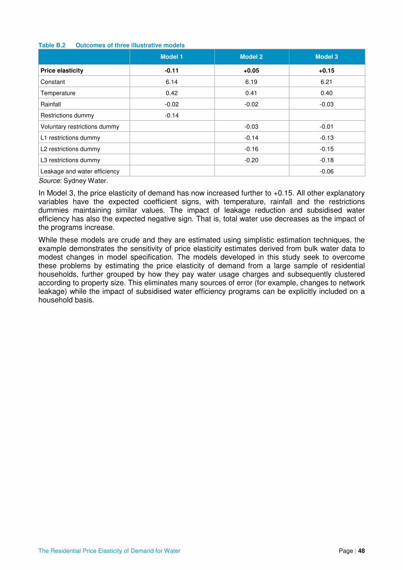
The Residential Price Elasticity of Demand for Water Page | 48
Table B.2 Outcomes of three illustrative models
Model 1 Model 2 Model 3
Price elasticity -0.11 +0.05 +0.15
Constant 6.14 6.19 6.21
Temperature 0.42 0.41 0.40
Rainfall -0.02 -0.02 -0.03
Restrictions dummy -0.14
Voluntary restrictions dummy -0.03 -0.01
L1 restrictions dummy -0.14 -0.13
L2 restrictions dummy -0.16 -0.15
L3 restrictions dummy -0.20 -0.18
Leakage and water efficiency -0.06
Source: Sydney Water.
In Model 3, the price elasticity of demand has now increased further to +0.15. All other explanatory variables have the expected coefficient signs, with temperature, rainfall and the restrictions dummies maintaining similar values. The impact of leakage reduction and subsidised water efficiency has also the expected negative sign. That is, total water use decreases as the impact of the programs increase.
While these models are crude and they are estimated using simplistic estimation techniques, the example demonstrates the sensitivity of price elasticity estimates derived from bulk water data to modest changes in model specification. The models developed in this study seek to overcome these problems by estimating the price elasticity of demand from a large sample of residential households, further grouped by how they pay water usage charges and subsequently clustered according to property size. This eliminates many sources of error (for example, changes to network leakage) while the impact of subsidised water efficiency programs can be explicitly included on a household basis.

The Residential Price Elasticity of Demand for Water Page | 49
Appendix C Advantages of using panel data
Some advantages of panel data are listed below:
1. More accurate inference of model parameters
Panel data contain more information and more sample variability than cross-sectional or time series data. This leads to more efficient estimates of the model parameters. Notice that a cross-sectional (time series) data set can be viewed as a panel with a single time period (individual).
2. Greater capacity for uncovering dynamic relationships
Economic behavior is inherently dynamic due to habit formation that underlies decision making, costs of adjustment and information uncertainty; as a result, households may respond to changes in the economic environment with a lapse of time. Thus, most economically interesting relationships are explicitly or implicitly dynamic. However, the estimation of time-adjustment patterns using time series data often requires to impose arbitrary prior restrictions, such as Koyck or Almon distributed lag models, given that time series observations of current and lagged variables are often highly collinear. With panel data, one can use the differences between households to alleviate collinearity and estimate time-adjustment patterns without any restrictions.
3. Providing micro foundations for aggregate data analysis
Aggregate data analysis often invokes the ‘representative agent’ assumption, which implies that all agents of the same type are identical.13 However, if agents (households) are heterogeneous, the time series properties of aggregate data be very different from those of disaggregate data (for example, see Granger (1990) or Pesaran (2003)). In addition, policy formulation and evaluation based on aggregate data may be grossly misleading.
In particular, as demonstrated in this study, households in owner occupied houses are more sensitive to changes in water usage prices compared to households in housing units. This is to be expected given the different way each household pays water usage charges. Aggregate time series analysis is likely to mask these differences and the resulting estimate of the average price elasticity of demand may well be biased.
In econometrics, this problem is known as ‘heterogeneity bias’ or ‘aggregation bias’. Panel data ‘follow’ a sample of households over time and therefore they are ideal for overcoming the issue of parameter heterogeneity.
4. Controlling for the impact of omitted variables
It is often argued that the main reason for finding (or not finding) certain effects of the explanatory variables is because there are omitted variables in one’s model specification, which are correlated with the explanatory variables. Since panel data contain information on both the intertemporal dynamics and the individuality of the households, they may allow one to control the effects of unobserved or omitted variables.
A popular example is a model of wage determination. Wage is a function not only of the level of education, experience and tenure with the current employer, among other factors, but it also depends on the level of innate ability or talent for a given individual. However, ‘talent’ is inherently unobserved and hard to quantify in any case; therefore, leaving it out of the model can lead to seriously biased inferences on the impact of education on wage since talent is likely to be correlated with education.
On the other hand, since an individual’s talent stays constant over time, the time dimension of the panel allows one to consider the difference of an individual’s wage over time, which eliminates the effect of talent on wage.
13 Sometimes the term is used by economists to refer to a situation in which agents differ, but act in such a way that
the sum of their choices is equivalent mathematically to the decision of a single individual.

The Residential Price Elasticity of Demand for Water Page | 50
In the context of the present report, water usage at the household level, aside from price, income and weather factors, depends on certain variables like lot size, household size and so on. With panel data it becomes possible to apply a transformation to the model that will eliminate the effect of time invariant variables on water usage. Thus, the rate of change of a household’s water usage will not depend on these variables. Therefore, estimating a model in first-differences may potentially provide unbiased estimates of the parameters, at least in large samples.
The effects of lot size and household size are not separately identifiable, because the rate of change of a household’s water usage does not depend on either of these factors. However, the main objective in this study is to obtain an unbiased (in large samples) estimate of the price elasticity of demand controlling for all other possible factors, some of which are unobserved.
5. Controlling for measurement errors
Panel data involve at least two dimensions, a cross-sectional dimension and a time series dimension. Thus, in certain cases, the availability of panel data simplifies computation and inference, particularly in models that are subject to measurement error. Measurement errors can create problems of identification of an econometric model (e.g. Aigner, Hsiao, Kapteyn and Wansbeek (1985)). However, the availability of multiple observations for a given household allows one to obtain more information and therefore potentially identify an otherwise unidentified model (e.g. Biorn (1992), and Wansbeek and Koning (1989)).
For example, in our context, income at the household level is unobserved. As a result, we use a proxy for income, the computation of which will be explained in the next section. This is a classic case where one of the regressors is measured inaccurately, that is, with some error. Panel data analysis allows us to use estimation techniques that can potentially circumvent this problem and provide unbiased estimates of the parameters, at least in large samples.

The Residential Price Elasticity of Demand for Water Page | 51
Appendix D Creating the dataset
A schematic diagram showing how households were selected for analysis is shown on the following page. Townhouses were not included in the analysis, which represent around 5 per cent of total residential demand.
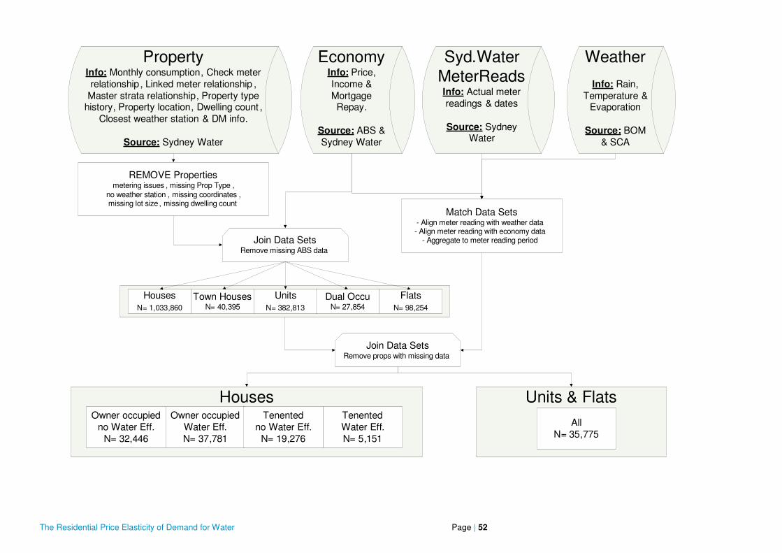
The Residential Price Elasticity of Demand for Water Page | 52
Houses
Weather
Info: Rain, Temperature &
Evaporation
Source: BOM & SCA
EconomyInfo: Price, Income & Mortgage Repay.
Source: ABS & Sydney Water
PropertyInfo: Monthly consumption, Check meter relationship, Linked meter relationship ,
Master strata relationship, Property type history, Property location, Dwelling count ,
Closest weather station & DM info.
Source: Sydney Water
REMOVE Propertiesmetering issues , missing Prop Type ,
no weather station , missing coordinates , missing lot size , missing dwelling count
Join Data SetsRemove missing ABS data
Syd.Water MeterReadsInfo: Actual meter readings & dates
Source: Sydney Water
HousesN= 1,033,860
Town HousesN= 40,395
UnitsN= 382,813
Join Data SetsRemove props with missing data
Dual OccuN= 27,854
FlatsN= 98,254
Match Data Sets- Align meter reading with weather data- Align meter reading with economy data
- Aggregate to meter reading period
Units & Flats
AllN= 35,775
Owner occupiedno Water Eff.
N= 32,446
TenentedWater Eff.N= 5,151
Owner occupiedWater Eff.N= 37,781
Tenentedno Water Eff.
N= 19,276

The Residential Price Elasticity of Demand for Water Page | 53
Appendix E Detail on model outputs
The timeframe of the analysis was from June 2004 to June 2009. For owner occupied and tenanted houses, the model is specified as follows:
,1 , ,2
lnln
4
1765
4321
5
01
<+=+⋅+⋅+⋅+⋅+
⋅+⋅+⋅+⋅+⋅+⋅+⋅=
∑
∑
=
= −−
αεηδγγγ
γγγγγβα
itiitj ititjjititit
itititititj jitjitit
uuseasonalleveldiywmachine
waterfixevaptemprainpdiwapricecc (E.1)
where:
lncit denotes the natural logarithm of average daily consumption of household i at time period t;
wapriceit denotes the weighted average water usage price calculated based on daily consumption;
pdiit is household disposable income;
rainit, tempit and evapit denote the deviation from the average value of rainfall, temperature and evaporation;
waterfixit, wmachineit and diyit denote participation in the three water efficiency programs; and
seasonalit is a set of variables that captures the effect of the season.
For housing units, the levels of temperature and rainfall were used rather than the deviations from the average together with seasonal variables (see Section 3).
The error term is composite and consists of ηi, which allows for unobserved household-specific effects that may be correlated with the explanatory variables, such as geographical location, size of the property, household size etc., and εit, which is the usual random noise component.
The above model is estimated separately for different user groups; in particular, for owner occupied households, tenanted houses and housing units. This allows the coefficients of the model to vary across these different household types. Furthermore, we allow the coefficients to vary according to whether households have engaged in a water efficiency program or not during the period of the analysis. Therefore, we estimate the model separately for these two cases.14 This is desirable because one can anticipate a different behavior towards changes in price for households that have already participated in water efficiency programs.
In addition, within each user group clusters of households were formed that are similar with respect to the size of the households’ property size. The model in (E.1) was estimated for each cluster specifically. The usefulness of this approach lies in that while the term ηi captures the direct impact of property size on water demand, it does not allow for variations in the price elasticity of demand associated with property size.
For owner occupied houses, 18 clusters were found for the households that did not participate in a water efficiency program and 31 clusters for households that did. For tenanted houses, seven clusters were found in both cases. Finally, housing units have one cluster since there is not much variation in property size in this case. Thus, 64 separate econometric models were estimated.
The coefficient β1 in (E.1) shows the expected effect of a unit change in water usage price on demand within the period that the change took place. Thus, β1 reflects the immediate or ‘short-run’ effect of a change in price. The full price effect is obtained by dividing the sum of the price coefficients, Σiβj, by 1-α. The resulting value is known as the ‘long-term’ or ‘long-run’ coefficient. The value of α has structural significance as it captures habit formation in water consumption and costs of adjustment – that is, it allows for the fact that in practice it takes time for households to adjust fully to a given change in water usage price at period t. For stability α is restricted within the interval (0,1). A high value of α indicates that the series is highly persistent; in other words, it takes relatively more time for the full impact of a change in price on demand to be realised. The rate of
14 Obviously for the case where households have not undertaken such a program we have γ4 = γ5= γ6 = 0.
The Residential Price Elasticity of Demand for Water Page | 54
adjustment towards the long-term or equilibrium value is given by 1-α. High values of α imply that the rate of adjustment is small.
Since the model is in semi-logarithmic form, the price elasticity of demand at the period where the price change took place is obtained by multiplying the coefficient, β1, with a range of values for price. Similarly the long-term elasticity is obtained by multiplying the long-term coefficient, Σiβj/(1-α), with a range of values for price. As a result, the higher the value of price is, the higher is the elasticity. Therefore, the functional form implies that consumers become more sensitive to price changes the higher the level of price is at first place. This result is consistent with utility theory.
To remove the effect of unobserved time-invariant household-specific heterogeneity, the model in (E.1) is transformed into first-differences. Therefore, the rate of change in water consumption becomes a function of the rate of change in water usage prices and the remaining control variables. The variables that do not vary over time are eliminated. Our focus lies on explaining changes in demand due to changes in price, controlling for other factors that may influence demand.
Estimation is performed using the Generalised Method of Moments (GMM) estimator developed originally by Hansen (1982) and extended for dynamic panel data models by Arellano and Bond (1991), Ahn and Schmidt (1995) and Blundell and Bond (1998), among others. GMM is a common choice when the explanatory variables are endogenous. In the present context the lagged dependent variable is endogenous by construction, since taking first-differences induces contemporaneous correlation between ∆lncit-1 and ∆εit. The weighted average water usage price is also endogenous because its value depends on water usage.
The appropriate lag length of the instruments used is determined by combining the outcome of the serial correlation test developed by Arellano and Bond (1991) with the outcome of Hansen’s test of overidentifying restrictions.
To illustrate our analysis, the following page shows the results obtained from estimating (E.1) for one cluster of owner occupied households that did not participate in a water efficiency program. Similar methodology was applied to all 64 models. Average estimates across the different user groups are reported in Table E.1.
The first set of results corresponds to estimates of the immediate expected response of water usage to changes in the explanatory variables, followed by estimates of the long-term response. For the former set of results, robust standard errors are reported, which are valid under arbitrary forms of heteroskedasticity and serial correlation. Furthermore, Windmeijer's (2005) correction of the finite-sample bias of the standard errors of the two-step GMM estimator is performed. For the long-term estimates standard errors are not directly available and therefore we have used the method of bootstrap to obtain these values. In particular, the procedure involved generating 1,000 samples by resampling from the current sample, estimating the long-term parameters each time and finally computing the standard error of the coefficients based on the standard deviation of these 1,000 estimates.
The GMM estimated parameters are statistically significant and have the expected sign in the immediate period and the long-term.15 The immediate price elasticity of demand is computed by multiplying -.000681 with a range of values for price. For example, at $1.20 per kL (expressed as cents per kL in the econometric models), the price elasticity of demand is about 8 per cent in the immediate period and 14 per cent in the long-term. The estimate of the autoregressive coefficient roughly equals 0.475which indicates that it takes about four time periods for ninety percent of the total effect of a change in price to be realised, all other things being constant. The estimated transition path is not smooth. Such outcome was common across the 64 econometric models. This result could be the due to various reasons, including further heterogeneity in the season and weather coefficients within clusters. Although there is merit in further research to try to understand better the nature of the transition path, it is worth emphasising that the estimates of the immediate or long-term price elasticity of demand are stable across a large range of the models estimated as well as across a different number of lags for price.
15 The coefficients of income and temperature were statistically insignificant and therefore they have been removed.

The Residential Price Elasticity of Demand for Water Page | 55

The Residential Price Elasticity of Demand for Water Page | 56
The estimated coefficient of rain deviation equals about -0.01 and -0.02 in the short- and long-term respectively. This can be interpreted as saying that if average daily rainfall is around 1 mm higher than average, demand is expected to fall by approximately one percent immediately and two percent in the long-term. Similarly, the estimated coefficient of evaporation deviation is approximately equal to 0.087 and 0.165 in the short and long-term, respectively. Thus, evaporation has a larger influence than rainfall.16
The coefficients of the seasonal variables are interpretable in relative terms. For example, in the short-run the difference between the coefficient of winter and summer is about -0.167. Therefore, one can argue that moving from summer to winter results on average in about 17 per cent reduction in average daily consumption, all else constant.17
Finally, the coefficient of Level 2 restrictions is positive, as expected, and its value indicates that moving from Level 2 to Level 3 restrictions resulted in about 1.7 per cent decrease in water usage, on average. Hence the effect is rather small.
We also report Hansen's test of overidentifying restrictions and Arellano and Bond's (1991) test of serial correlation of the disturbances, up to third order. The former is used to determine empirically the validity of the overidentifying restrictions in the GMM model. The null hypothesis is that the model is correctly specified. This is not rejected at the 1 per cent level of significance. The latter is useful because it provides an indication of the appropriate lag length of the instruments to be used, since instruments are required to be orthogonal to the error term. Some serial correlation of first-order is expected due to first-differencing of the data, which is essentially why the null hypothesis is rejected in this case. However, it is clear that the null hypotheses of no serial correlation of up to second and third order are not rejected, which indicates that instruments with respect to three or further lags of the dependent variable are suitable.
At the bottom of the results we report the outcome of Davidson and MacKinnon’s (1981) statistic for testing between non-nested models. The null hypothesis is that the semi log model is preferred over the double log specification. As it is clear, this is not rejected by the data at the 1 per cent level of significance.
Table E.1 reports the weighted average estimates across clusters for different segments of the market. The number of households existing within each cluster determines the weights.
16 The coefficient of temperature was statistically insignificant. This implies that once the effect of evaporation is taken
into account, temperature does not have an extra effect on water usage. 17
We can obtain a more accurate estimate by exponentiating the difference between the two coefficients and
subtracting the value of one. This yields -.154, i.e. a -15.4%. reduction implied by moving from summer to winter.
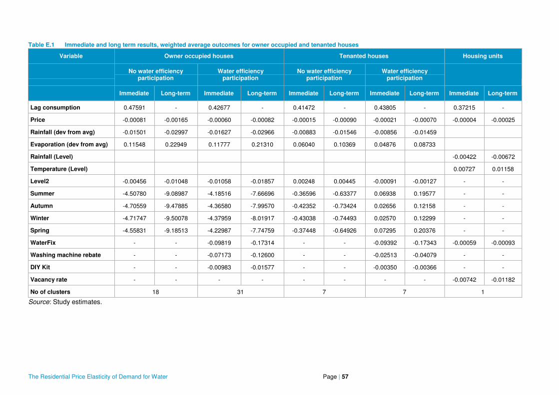
The Residential Price Elasticity of Demand for Water Page | 57
Table E.1 Immediate and long term results, weighted average outcomes for owner occupied and tenanted houses
Variable Owner occupied houses Tenanted houses Housing units
No water efficiency participation
Water efficiency participation
No water efficiency participation
Water efficiency participation
Immediate Long-term Immediate Long-term Immediate Long-term Immediate Long-term Immediate Long-term
Lag consumption 0.47591 - 0.42677 - 0.41472 - 0.43805 - 0.37215 -
Price -0.00081 -0.00165 -0.00060 -0.00082 -0.00015 -0.00090 -0.00021 -0.00070 -0.00004 -0.00025
Rainfall (dev from avg) -0.01501 -0.02997 -0.01627 -0.02966 -0.00883 -0.01546 -0.00856 -0.01459
Evaporation (dev from avg) 0.11548 0.22949 0.11777 0.21310 0.06040 0.10369 0.04876 0.08733
Rainfall (Level) -0.00422 -0.00672
Temperature (Level) 0.00727 0.01158
Level2 -0.00456 -0.01048 -0.01058 -0.01857 0.00248 0.00445 -0.00091 -0.00127 - -
Summer -4.50780 -9.08987 -4.18516 -7.66696 -0.36596 -0.63377 0.06938 0.19577 - -
Autumn -4.70559 -9.47885 -4.36580 -7.99570 -0.42352 -0.73424 0.02656 0.12158 - -
Winter -4.71747 -9.50078 -4.37959 -8.01917 -0.43038 -0.74493 0.02570 0.12299 - -
Spring -4.55831 -9.18513 -4.22987 -7.74759 -0.37448 -0.64926 0.07295 0.20376 - -
WaterFix - - -0.09819 -0.17314 - - -0.09392 -0.17343 -0.00059 -0.00093
Washing machine rebate - - -0.07173 -0.12600 - - -0.02513 -0.04079 - -
DIY Kit - - -0.00983 -0.01577 - - -0.00350 -0.00366 - -
Vacancy rate - - - - - - - - -0.00742 -0.01182
No of clusters 18 31 7 7 1
Source: Study estimates.
The Residential Price Elasticity of Demand for Water Page | 58
Abbreviations
ABS Australian Bureau of Statistics
ARDL model Autoregressive, distributed lag model
BoM Bureau of Meteorology
CCD Census collection district
DIY kits ‘Do it yourself’ kits
GMM Generalised method of moments
IPART Independent Pricing and Regulatory Tribunal
KL Kilolitre
LPD Litres per person per day
ML Maximum likelihood
OLS Ordinary least squares

The Residential Price Elasticity of Demand for Water Page | 59
Glossary
Bulk water Total water inputted into a water distribution network. It includes both metered and unmetered water
Drought restrictions Mandatory restrictions on the type, method and time people can undertake outdoor water use
Gigalitre Equal to one thousand megalitres
Kilolitre Equal to one thousand litres
Long run marginal cost The expected cost of bringing forward an extra unit of supply in the long term, including associated capital expenditure for infrastructure.
Megalitre Equal to one thousand kilolitres
Price elasticity of demand The responsiveness of demand to changes in price. It is calculated as the percentage change in demand due divided by the percentage change in price
Scarcity pricing A charge that reflects the value of water in alternative uses during periods of water shortages.
Short run marginal cost The cost of providing an additional unit of supply to meet demand in the short term, reflecting the highest value use to which a commodity can be put in periods of shortage.
Water conservation activities Includes leak reduction, water efficiency programs and recycling

The Residential Price Elasticity of Demand for Water Page | 60
References
Ahn, S.C. and Schmidt, P. (1995), ‘Efficient Estimations of Models for Dynamic Panel Data’, Journal of Econometrics, 68, 5-28.
Aigner, D.J., C. Hsiao, A. Kapteyn and T. Wansbeek (1985), ‘Latent Variable Models in Econometrics’, Handbook of Econometrics, vol. II, ed. by Z. Griliches and M.D. Intriligator, Amsterdam: North-Holland, 1322-1393.
Al-Qunaibet, M, H. and R. S. Johnston (1985), ‘Municipal Demand for Water in Kuwait: Methodological Issues and Empirical Results’, Water Resources Research, Vol. 21 (4), 433-438.
Arellano, M. and Bond S. (1991), ‘Some Tests of Specification for Panel Data: Monte Carlo Evidence and an Application to Employment Equations’, Review of Economic Studies, 58, 277-297.
Barker, A., Murray, T. and Salerian, J. (2010), Developing a Partial Equilibrium Model of an Urban Water System, Staff Working Paper, Melbourne, March.
Blundell, R. and Bond, S. (1998), ‘Initial Conditions and Moment Restrictions in Dynamic Panel Data Models’, Journal of Econometrics, 87, 115-143.
Biorn, E. (1992), ‘Econometrics of Panel Data with Measurement Errors’, Econometrics of Panel Data: Theory and Applications, ed. by. L. Matyas and P. Sevestre, Klumer, 152-195.
Davidson, R. and MacKinnon, J.G. (1981), ‘Several Tests for Model Specification in the Presence of Alternative Hypotheses, Econometrica, 49, 781-793.
Everitt, B. (2003), ‘Cluster analysis’, 3rd ed., London: Eward Arnold.
Grafton, R and T. Kompas (2007) ‘Pricing Sydney Water’, The Australian Journal of Agricultural and Resource Economics, 51, pp. 227.241.
Grafton, R and Ward, M (2007) ‘Prices versus rationing: Marshallian surplus and mandatory water restrictions’, ANU Economics and Environment Networks Working Paper, Canberra.
Granger, C.W.J. (1990), ‘Aggregation of Time-Series Variables: A Survey’, Disaggregation in Econometric Modeling, ed. by T. Barker and M.H. Pesaran, London, Routledge.
Henry, Dr Ken (2008) Secretary to the Treasury, 2008, ‘Realising the Vision’, Speech to the Ian Little Memorial Lecture, Melbourne, 4 March.
Hall. A. (2005). ‘Generalized Method of Moments’, Oxford: Oxford University Press.
Hansen, L. P. (1982), ‘Large Sample Properties of Generalized Method of Moments Estimators’, Econometrica, 50, 1029-1054.
Howe, C.W. and Linaweaver, F.P. (1967), ‘The impact of price on residential water demand and its relation to system design and price structure’, Water Resources Research, 3, 13-32.
Infrastructure Australia (IA) 2010, Review of urban water security strategies, May
Lewbel, A. (1994), ‘Aggregation and Simple Dynamics’, American Economic Review, 84, 905-918.
Pesaran, M.H. (2003), ‘On Aggregation of Linear Dynamic Models: An Application to Life-Cycle Consumption Models Under Habit Formation’, Economic Modeling, 20, 227-435.
Productivity Commission (PC) (2008) Towards Urban Water Reform: A Discussion Paper, Productivity Commission Research Paper, Melbourne, March
Mátyás, L. (1999), ‘Generalized Method of Moments Estimation’, Cambridge: Cambridge University Press.
National Water Commission (NWC) (2008), Position Statement on urban water pricing, 2 July.
Nordin, J.A. (1976), ‘A Proposed Modification of Taylor's Demand Analysis: Comment’, The Bell Journal of Economics, 7, 719-21.

The Residential Price Elasticity of Demand for Water Page | 61
Sarafidis, V. (2006), ‘Estimating Panel Data Models with Cross-sectional Dependence’, Dissertation, University of Cambridge.
Sarafidis, V. and N. Weber (2010), ‘A Partially Heterogeneous Framework for Analysing Panel Data’, unpublished manuscript. An earlier working version of the paper can be found in: http://mpra.ub.uni-muenchen.de/20814/1/MPRA_paper_20814.pdf
Taylor, L.D. (1975), ‘The Demand for Electricity: A Survey’, The Bell Journal of Economics, 6, 74-110.
Wansbeek, T.J. and R.H. Koning (1989), ‘Measurement Error and Panel Data’, Statistica Neerlandica, 45, 85-92.
Warner, R (1996) Water pricing and the marginal cost of water. Occasional Paper No1. Urban Water Research Association of Australia, Melbourne.
Wendel, M. and Kamakura W. (1999), ‘Market Segmentation: Conceptual and Methodological Foundations, 2nd ed., Massachusetts: Kluwer Academic Publishers.
Windmeijer, F. (2005), ‘A Finite Sample Correction for the Variance of a Linear Efficient Two-step GMM Estimators, Journal of Econometrics, 126, 25-51.