The Reliability of Subjective Well-Being Measures · display a serial correlation of about 0.60...

The Reliability of Subjective Well-Being Measures

Alan B. Krueger Princeton University

David A. Schkade University of California, San Diego

First Draft: August 2006 This Draft: January 2007

The authors thank our colleagues Daniel Kahneman, Norbert Schwarz, and Arthur Stone for helpful comments and the Hewlett Foundation, the National Institute on Aging, and Princeton University’s Woodrow Wilson School for financial support.

Reliability of SWB Measures – 2

Introduction

Economists are increasingly analyzing data on subjective well-being. Since 2000, 157

papers and numerous books have been published in the economics literature using data on life

satisfaction or subjective well-being, according to a search of Econ Lit.1 Here we analyze the

test-retest reliability of two measures of subjective well-being: a standard life satisfaction

question and affective experience measures derived from the Day Reconstruction Method

(DRM). Although economists have longstanding reservations about the feasibility of

interpersonal comparisons of utility that we can only partially address here, another question

concerns the reliability of such measurements for the same set of individuals over time. Overall

life satisfaction should not change very much from week to week. Likewise, individuals who

have similar routines from week to week should experience similar feelings over time. How

persistent are individuals’ responses to subjective well-being questions? To anticipate our main

findings, both measures of subjective well-being (life satisfaction and affective experience)

display a serial correlation of about 0.60 when assessed two weeks apart, which is lower than the

reliability ratios typically found for education, income and many other common micro economic

variables (Bound, Brown, and Mathiowetz, 2001 and Angrist and Krueger, 1999), but high

enough to support much of the research that has been undertaken on subjective well-being.

The life satisfaction question that we examine is almost identical to that used in the

World Values Survey, and similar to that used in many other surveys. The DRM is a recent

development in the measurement of the affective experience of daily life. The gold standard for

such measurements is the Experience Sampling Method (ESM) (also called Ecological

Momentary Assessment (EMA)), in which participants are prompted at irregular intervals to

1 Prominent examples are Layard (2005), Blanchflower and Oswald (2004), and Frey and Stutzer (2002).


record their current circumstances and feelings (Csikszentmihalyi & Larsen, 1987; Stone,

Shiffman & DeVries, 1999). This method of measuring affect minimizes the role of memory

and interpretation, but it is expensive and difficult to implement in large samples. Consequently,

we use the Day Reconstruction Method (DRM), in which participants are required to think about

the preceding day, break it up into episodes, and describe each episode by selecting from several

menus (Kahneman, Krueger, Schkade, Schwarz, & Stone, 2004). The DRM involves memory,

but it is designed to increase the accuracy of emotional recall by inducing retrieval of the

specifics of successive episodes (Robinson & Clore, 2002; Belli, 1998). Evidence that the two

methods can be expected to yield similar results was presented earlier for subpopulation averages

(Kahneman, et al., 2004). A critical advantage of the DRM is that it provides data on time-use –

a valuable source of information in its own right, which has rarely been combined with the study

of subjective well-being.

In this paper we examine reliability measures for a sample of 229 women who each filled

out a DRM questionnaire for two Wednesdays, two weeks apart in 2005. We compare these

reliabilities to those of global well-being measures more typical in the literature, and we

decompose the reliability of duration-weighted net affect into a component due to the similarity

of activities across days and other factors. We also use these reliability estimates to correct

observed relationships between reported well-being and other variables (e.g., income) for

attenuation. We conclude with a discussion of the implications of measurement error for DRM

studies and for well-being research more generally.


What is reliability and why should we care?

Consider an observed variable, y, which is a noisy measure of the variable of interest, y*.

We can write where yi is the observed value for individual i, is the “correct”

value, and ei is the error term. Under the “classical measurement error” assumptions, ei is a

white noise disturbance that is uncorrelated with and homoskedastic. Classical measurement

error will lead correlations between y and other variables to be attenuated toward 0 in large

samples.

iii eyy += * *iy

*iy

2 If we can measure yi at two points in time, and if the measurement errors are

independent and have a constant variance over time, then the correlation between the two

measures provides an estimate of the ratio of the variance in the signal to the total variance in y.

We thus define the reliability ratio, r, as r = , where the superscripts indicate the

measurement taken in periods 1 and 2. Under the assumptions stated,

),( 21ii yycorr

var(e) (y*)var var(y*) =r plim

+.

In addition to summarizing the extent of random noise in subjective well-being reports,

the signal-to-total variance ratio is of interest because, in the limit, it equals the proportional bias

that arises when SWB is an explanatory variable in a bivariate regression. Furthermore, as we

explain below, correlations between SWB and other variables are attenuated by random

measurement error in SWB. An important application of SWB data involves estimating the

correlation between life satisfaction, affect and other variables such as income (e.g., Argyle,

1999). We can use the reliability ratio to correct those correlations for attenuation.

Of course, if the measurement error is not classical, the test-retest correlation can under-

or over-state the signal-to-total variance ratio, depending on the nature of the deviation from

classical measurement error. With only two reports of y, and without knowledge of y*, it is not

2 If y is of limited range (e.g., a binary variable) than e will necessarily be correlated with y*. We ignore this issue for the time being.


possible to assess the plausibility of the classical measurement error assumptions. If the errors in

measurement are positively correlated over time, then the test-retest correlation will overstate the

reliability of the data. Nevertheless, the test-retest correlation is a convenient starting point for

assessing the reliability of subjective well-being data.

Related literature

There is a vast empirical literature on subjective well being (Kahneman, Diener and

Schwarz, 1999). Subjective well-being is most commonly measured by asking people a single

question, such as, “All things considered, how satisfied are you with your life as a whole these

days?” or “Taken all together, would you say that you are very happy, pretty happy, or not too

happy?” Such questions elicit a global evaluation of one’s life. Surveys in many countries

conducted over decades indicate that, on average, reported global judgments of life satisfaction

or happiness have not changed much over the last four decades, in spite of large increases in real

income per capita. Although reported life satisfaction and household income are positively

correlated in a cross section of people at a given time, increases in income have been found to

have mainly a transitory effect on individuals’ reported life satisfaction (Easterlin, 1995).

Moreover, the correlation between income and subjective wellbeing is notably weaker when a

measure of experienced happiness is used instead of life satisfaction (Kahneman et al., 2006). Of

course, such low correlations could be partially due to attenuation, if measurement error is high.

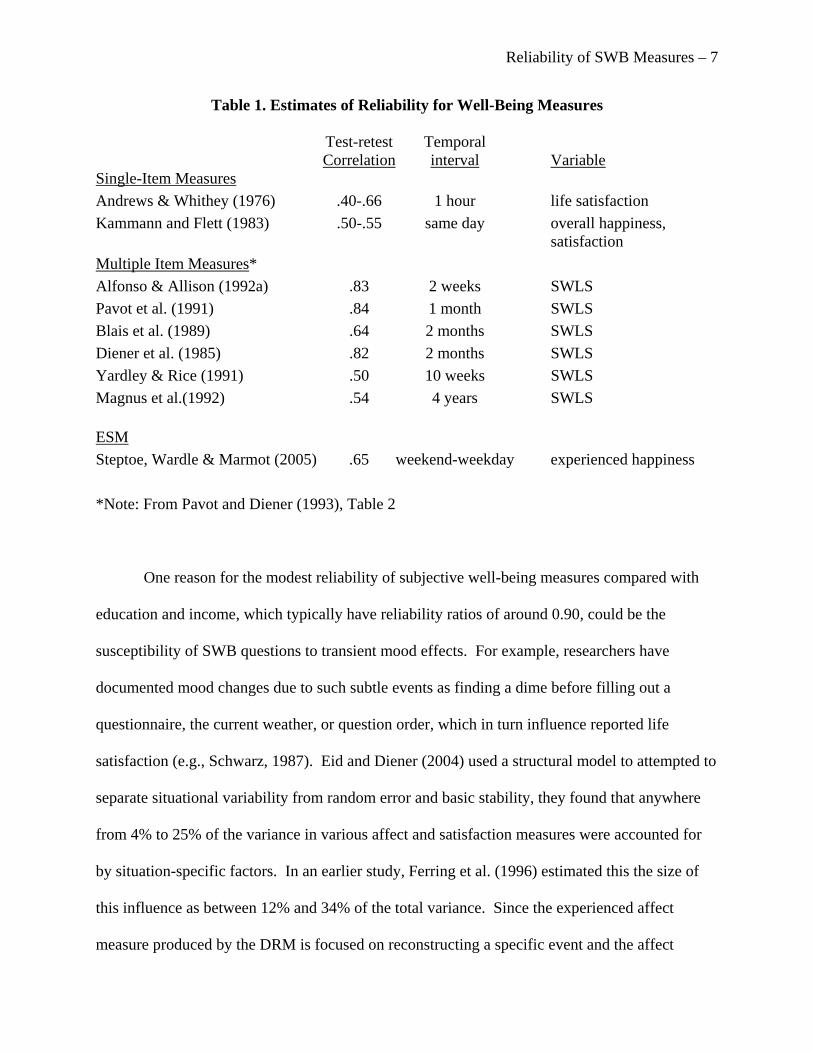
There is a small literature assessing the reliability of individual-level single-item well-

being measures, even less on the reliability of ESM, and none as of yet on the DRM (see Table

1). Single-item measures of SWB have been found to have relatively low reliabilities, usually

between .40 and .66, even when asked twice in the same session one hour apart (Andrews and


Whithey, 1976). Kammann and Flett (1983) found that single-item well-being questions under

the instructions to consider “the past few weeks” or “these days” had reliabilities of .50 to .55

when asked within the same day. Interestingly, the only study we are aware of that looked at the

reliability of an ESM measure of duration-weighted happiness found a correlation on the upper

end of the range found for single-item global well-being measures (Steptoe, Wardle and Marmot,

2005). Overall, there has been surprisingly little attention paid to reliability, despite the wide use

of these measures.

The Satisfaction with Life Scale (SWLS, Diener et al., 1985) is another commonly used

global satisfaction measure. In contrast to the single question measures it consists of the average

of five related items, each of which is rated on a 7-point scale from Strongly Disagree (1) to

Strongly Agree (7). The items are: “In most ways my life is close to my ideal”; “The conditions

of my life are excellent”; “I am satisfied with my life”; “So far I have gotten the important things

I want in life”; and “If I could live my life over, I would change almost nothing”. A key reason

that SWLS has proven more reliable than single item questions (see Table 1), is that since it is

the sum of multiple items, it benefits from error reduction through aggregation. Eid and Diener

(2004) used a structural model to estimate reliability for a sample of 249 students, measured

three times with four weeks between successive measurements. After statistically separating out

the influence of situation specific factors, they estimated that the imputed stability for life

satisfaction was very high, around 0.90.


Table 1. Estimates of Reliability for Well-Being Measures Test-retest Temporal Correlation interval Variable Single-Item Measures Andrews & Whithey (1976) .40-.66 1 hour life satisfaction Kammann and Flett (1983) .50-.55 same day overall happiness, satisfaction Multiple Item Measures* Alfonso & Allison (1992a) .83 2 weeks SWLS Pavot et al. (1991) .84 1 month SWLS Blais et al. (1989) .64 2 months SWLS Diener et al. (1985) .82 2 months SWLS Yardley & Rice (1991) .50 10 weeks SWLS Magnus et al.(1992) .54 4 years SWLS ESM Steptoe, Wardle & Marmot (2005) .65 weekend-weekday experienced happiness *Note: From Pavot and Diener (1993), Table 2

One reason for the modest reliability of subjective well-being measures compared with

education and income, which typically have reliability ratios of around 0.90, could be the

susceptibility of SWB questions to transient mood effects. For example, researchers have

documented mood changes due to such subtle events as finding a dime before filling out a

questionnaire, the current weather, or question order, which in turn influence reported life

satisfaction (e.g., Schwarz, 1987). Eid and Diener (2004) used a structural model to attempted to

separate situational variability from random error and basic stability, they found that anywhere

from 4% to 25% of the variance in various affect and satisfaction measures were accounted for

by situation-specific factors. In an earlier study, Ferring et al. (1996) estimated this the size of

this influence as between 12% and 34% of the total variance. Since the experienced affect

measure produced by the DRM is focused on reconstructing a specific event and the affect


actually experienced during it, there is at least the possibility that such measures will be less

vulnerable to current mood at the time of the interview.

We might expect DRM measures to be less reliable over time than life satisfaction

because a person’s activities change from day to day. At the same time, DRM measures are

averages of multiple responses, while global life satisfaction of happiness is often assessed with

just one question. If ESM is any guide, the DRM may be at least as reliable as reported overall

life satisfaction.

Method

We evaluate the test-retest reliability of the DRM by having the same respondents

complete a DRM questionnaire two weeks apart regarding the same day of the week

(Wednesday). The questionnaire, which is available from the authors on request, also contained

standard global life satisfaction measures. The resulting data provide information about the

relative stability of the DRM compared to the types of global life satisfaction questions used in

most well being research for the same sample.

For comparability with our previous studies, the respondents (n = 229) were selected by

random selection of women from the driver’s license list in Travis County, Texas and screening

for employment and age between 18 and 60. Respondents were paid $50 upon completing the

first questionnaire and an additional $100 upon completing the second one for a total of $150.

The interview dates were two Thursdays, March 31, 2005 and April 14, 2005. Following the

DRM procedure, participants reported on the previous day. Completion times for the self-

administered instrument ranged from 45 to 75 min. The ethnic composition of the sample was


67% white (non-Hispanic), 7% African American, 21% Hispanic, and 5% other. Average age

was 42.8 years. Median household income category was $40,000-$50,000.

The DRM protocol described by Kahneman et al. (2004) was followed. Groups of

participants were invited to a central location for a session on Thursday evening, where they

answered a series of questions contained in four packets. The first packet included general

satisfaction and demographic questions. Next, the respondents were asked to construct a diary of

the previous day (Wednesday) as a series of episodes, noting the content and the beginning and

end time of each. In the third packet, they were asked for a detailed description of every episode

as explained below. The average number of episodes a respondent described for the day was

somewhat higher in the second session (14.8 vs 13.2, p < .001, by a paired t-test) although the

total time covered by the episodes was no different (16.8 vs 16.7 hrs, p > .20, by a paired t-test).

These figures compare to the 14.1 episodes and 15.4 hours reported in Kahneman et al. (2004).

The first few questions in the survey were global SWB questions. First was the overall

life satisfaction question, “Taking all things together, how satisfied are you with your life as a

whole these days? Are you very satisfied, satisfied, not very satisfied, not at all satisfied?”

Next, similar questions were asked for “your life at home” and “your present job”. Two global

mood questions followed, for home and for work. The question posed was ‘‘When you are at

home, what percentage of the time are you in a bad mood____%, a little low or irritable____%,

in a mildly pleasant mood____%, in a very good mood____%." The last two response categories

were added together to obtain the percentage of time in a good mood. Net mood was computed

by subtracting the sum of the first two response categories from the sum of the last two. The

same procedure was applied to the work mood question.


The affect measures derived from the DRM are combinations of the duration-weighted

affective adjectives that respondents rated for each episode. Net affect was computed by

subtracting the average of negative affect (NA) – tense/stressed, depressed/blue and angry/hostile

from the average of positive affect (PA) – happy, affectionate/friendly and calm/relaxed. 3

Difmax is the duration-weighted average of happy less the maximum of tense/stressed,

depressed/blue, angry/hostile. The U-index is closely related to Difmax, and equals one when

Difmax < 0 and = 0 otherwise. Intuitively, the U-index is an binary variable indicating the

proportion of time that an individual spends in a state in which the strongest emotion is a

negative one. Difmax and the U-index are recently proposed summary measures of affective

experience (Kahneman & Krueger, 2006; Kahneman, Schkade, Krueger, Fischler & Krilla,

2006).

Results

Table 2 presents the correlations between various measures for the same person in the

first and second sessions, as well as 95% confidence intervals. We focus first on overall

measures of affective experience. Perhaps the most surprising finding is that the reliabilities of

Net Affect (r=.64) and Difmax (r=.60) are at least as high as that for life satisfaction (r=.59).

Satisfaction with domains of life (work and home) are both more reliable than satisfaction with

life overall. The corresponding home and work mood measures are also more reliable than life

satisfaction. Another notable feature of the results is that positive affect appears to be somewhat

more reliable than negative affect.

3 Frustrated was excluded from negative affect for comparability with our other studies.


Table 2. Correlations Between Selected Measures at Period 1 and Period 2 95% confidence interval Observed Lower Upper Global Measures Life satisfaction .59 .49 .67 Home satisfaction .74 .68 .80 Work Satisfaction .68 .61 .75 Home net mood .70 .63 .76 Work net mood .68 .61 .75

Experience Measures Net affect .64 .56 .71 Difmax .60 .51 .68 Uindex .50 .40 .59

Positive Affect happy .62 .54 .70 affectionate/friendly .68 .61 .75 calm/relaxed .56 .46 .64 PA .68 .61 .75

Negative Affect tense/stressed .54 .44 .62 depressed/blue .60 .51 .68 angry/hostile .54 .44 .63 frustrated .48 .37 .57 NA .60 .51 .68

Other affect adjectives impatient for it to end .56 .47 .65 competent/doing well .64 .55 .71 interested/focused .57 .47 .65 tired .65 .56 .72

Demographics Household income .96 .95 .97 Education (yrs) .98 .98 .99 Age 1.00 1.00 1.00 __________________________________

Note: Confidence intervals for the correlations are not symmetric because they are based on the nonlinear Fisher’s z transformation (z = .5[ln(1+r) - ln(1-r)]), which is normally distributed and used for significance testing. Sample sizes are 228 or 229, except for age, which is 223 due to missing data.


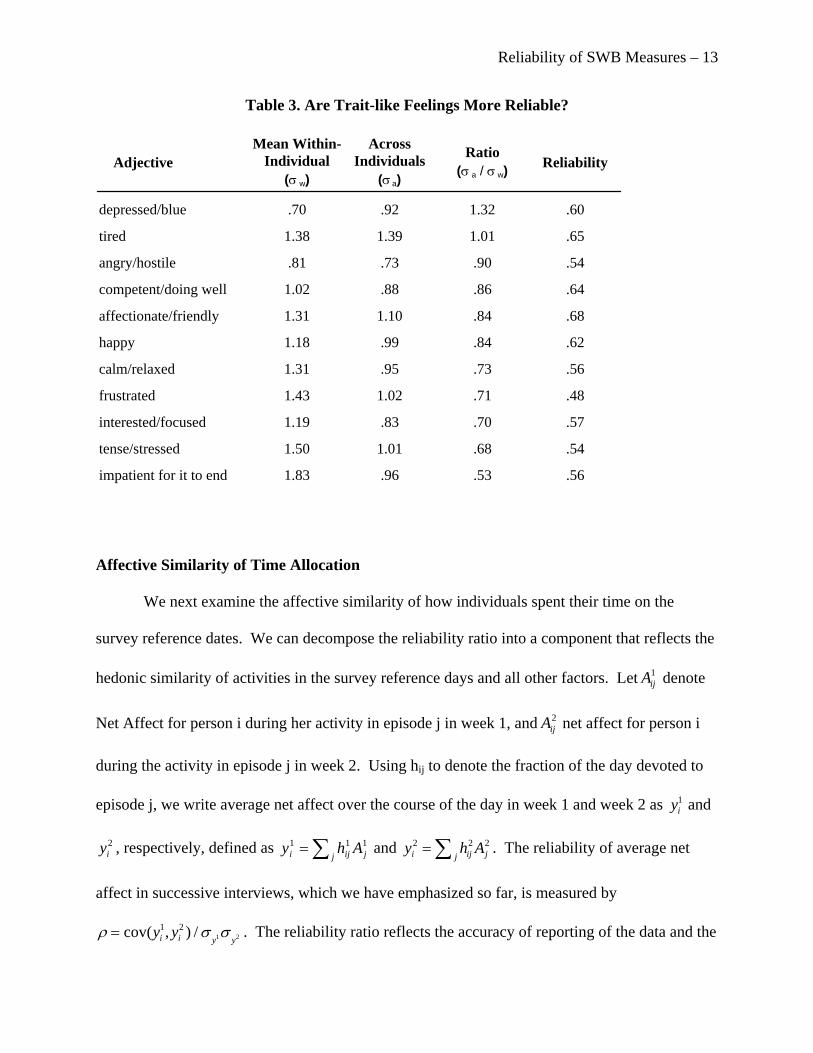
The extent to which a person’s rating of a particular adjective over different episodes of

the day represents personal traits or is influenced by the variability in situations is likely related

to the reliability of that adjective. If a given person tends to feel the same way most of the time

(a “happy” person or a “depressed” person) regardless of the situation, then this adjective might

be expected to have greater reliability across the two sessions, since the activities the person

engages in on the two days vary. To crudely gauge the extent to which particular adjectives are

person-bound or situation-bound, for each adjective we pooled the two sessions and computed

the variance of the duration-weighted personal averages across people and the average variance

within each person’s days across episodes, and then took the ratio of the between people to

within-person variances. A high ratio would indicate that an adjective is relatively constant for a

person (more of an individual difference like a trait) and a low ratio would indicate that an

adjective is determined more by the situation than who the person is. Results are shown in Table

3. Quite plausibly, feeling depressed appears to be a more trait-like descriptor, while feeling

tense/stressed or impatient for an episode to end are highly situational. Interestingly, we found a

correlation of 0.41 between the variance ratio and the reliability ratios shown in Table 3, which

indicates moderate support for the hypothesis of greater reliability for trait-like emotions.4

4 We also computed these ratios for the DRM sample in Kahneman et al (2004). The two samples produced very similar sets of ratios – for the 8 adjectives in common between the two samples the correlation of the ratios was .89.


Table 3. Are Trait-like Feelings More Reliable?

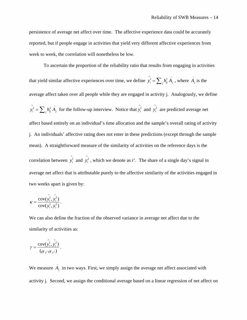
ffective Similarity of Time Allocation

We next examine the affective similarity of how individuals spent their time on the

survey reference dates. We can decompose the reliability ratio into a component that reflects the

hedonic similarity of activities in the survey reference days and all other factors. Let denote

Net Affect for person i during her activity in episode j in week 1, and net affect for person i

during the activity in episode j in week 2. Using hij to denote the fraction of the day devoted to

episode j, we write average net affect over the course of the day in week 1 and week 2 as and

, respectively, defined as and

AdjectiveMean Within-

Individual (σ w)

Across Individuals

(σ a)

Ratio (σ a / σ w) Reliability

depressed/blue .70 .92 1.32 .60

tired 1.38 1.39 1.01 .65

angry/hostile .81 .73 .90 .54

competent/doing well 1.02 .88 .86 .64

affectionate/friendly 1.31 1.10 .84 .68

happy 1.18 .99 .84 .62

calm/relaxed 1.31 .95 .73 .56

frustrated 1.43 1.02 .71 .48

interested/focused 1.19 .83 .70 .57

tense/stressed 1.50 1.01 .68 .54

impatient for it to end 1.83 .96 .53 .56

A

1ijA

2ijA

1iy

2iy 111

jj iji Ahy ∑= 222jj iji Ahy ∑=

have emphasized so far, is m

. The reliability of average net

affect in successive interviews, which we easured by

. The reliability ratio reflects the accuracy of reporting of the data and the ρ = cov(yi1, yi

2 ) / σy1σ y2


persistence of average

that results from engaging in activities

that yie

ity

in

net affect over time. The affective experience data could be accurately

reported, but if people engage in activities that yield very different affective experiences from

week to week, the correlation will nonetheless be low.

To ascertain the proportion of the reliability ratio

ld similar affective experiences over time, we define _

11jj iji Ahy ∑=

∧

, where _

jA is the

average affect taken over all people while they are engaged in

_22

jj iji Ahy ∑=∧

for the follow-up interview. Notice that∧1iy and

∧2iy are predicted average net

tirely on an individual’s time allocation a the s ple’s overall rating of activ

j. An individuals’ affective rating does not enter in these predictions (except through the sample

mean). A straightforward measure of the similarity of activities on the reference days is the

correlation between ∧1iy and

∧2iy , which we denote as r’. The share of a single day’s signal in

average net affect that is attributable purely to the affective similarity of the activities engaged

two weeks apart is given by:

activity j. Analogously, we define

affect based en nd am

),cov(),cov( 21

ii yy∧∧

=κ . 21ii yy

We can also define the fraction of the observed variance in average net affect due to the

similarity of activities as:

)(),cov( 21

γ ii yy∧∧

= . 21 σσ yy

We measure in two ways. First, we simply assign the average net affect associated with

activity j. Second, we assign the conditional average based on a linear regression of net affect on

_

jA


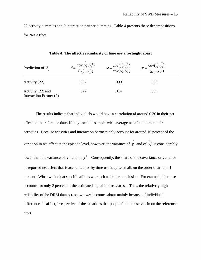
22 activity du ies and 9 interaction partner dummies. Table 4 presents these decompositionmm s

for Net Affect.

Table 4: The affective similarity of time use a fortnight apart

rediction of _

jA ),(),cov(

'21

21

σσ ∧∧

∧∧

=),cov(),cov(

21

21

ii

ii

yyyy∧∧

=κ )(),cov(

21

21

σσγ

yy

ii yy∧∧

= Pii yy

ii yyr

Activity (22) .267 .009 .006

.322 .014 .009 Interaction Partner (9)

indicate that individuals would have a correlation of around 0.30 in their net

ffect on the reference dates if they used the sample-wide average net affect to rate their

ctivities. Because activities and interaction partners only account for around 10 percent of the

iderably

percent. When we look at specific affects we reach a similar conclusion. For example, time use

accounts for only 2 percent of the estimated signal in tense/stress. Thus, the relatively high

reliability of the DRM data across two weeks comes about mainly because of individual

differences in affect, irrespective of the situations that people find themselves in on the reference

days.

Activity (22) and

The results

a

a

variation in net affect at the episode level, however, the variance of iy and of iy is cons

lower than the variance of 1 and of 2 . Consequently, the share of the covariance or variance

of reported net affect that is accounted for by time use is quite small, on the order of around 1

∧1

∧2

iy iy


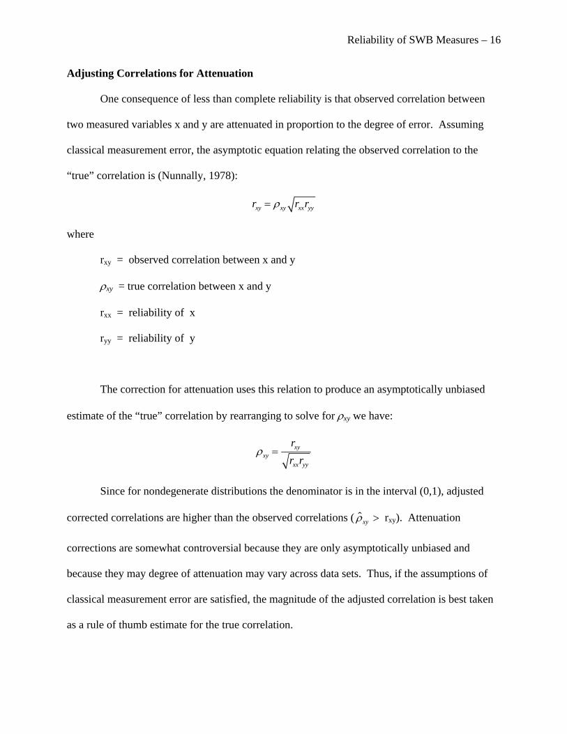
Adjusting Correlations for Attenuation

One consequence of less than complete reliability is that observed correlation between

o measured variables x and y are attenuated in proportion to the degree of error. Assuming

equation relating the observed correlation to the

“true” c

tw

classical measurement error, the asymptotic

orrelation is (Nunnally, 1978):

rxy = ρxy rxxryy

where

r = observed correlation betwxy een x and y

ρxy = true correlation between x and y

rxx = reliability of x

nuation uses this relation to produce an asymptotically unbiased

estimat ion by rearranging to solve for ρxy we have:

ryy = reliability of y

The correction for atte

e of the “true” correlat

ρxy =rxy

rxxryy

rval (0,1), adjusted

corrected correlations are higher than the observed correlations (

Since for nondegenerate distributions the denominator is in the inte

ρ̂xy > rxy). Attenuation

corrections are somewhat controversial because they are only asymptotically unbiased and

because

jus taken

they may degree of attenuation may vary across data sets. Thus, if the assumptions of

classical measurement error are satisfied, the magnitude of the ad ted correlation is best

as a rule of thumb estimate for the true correlation.


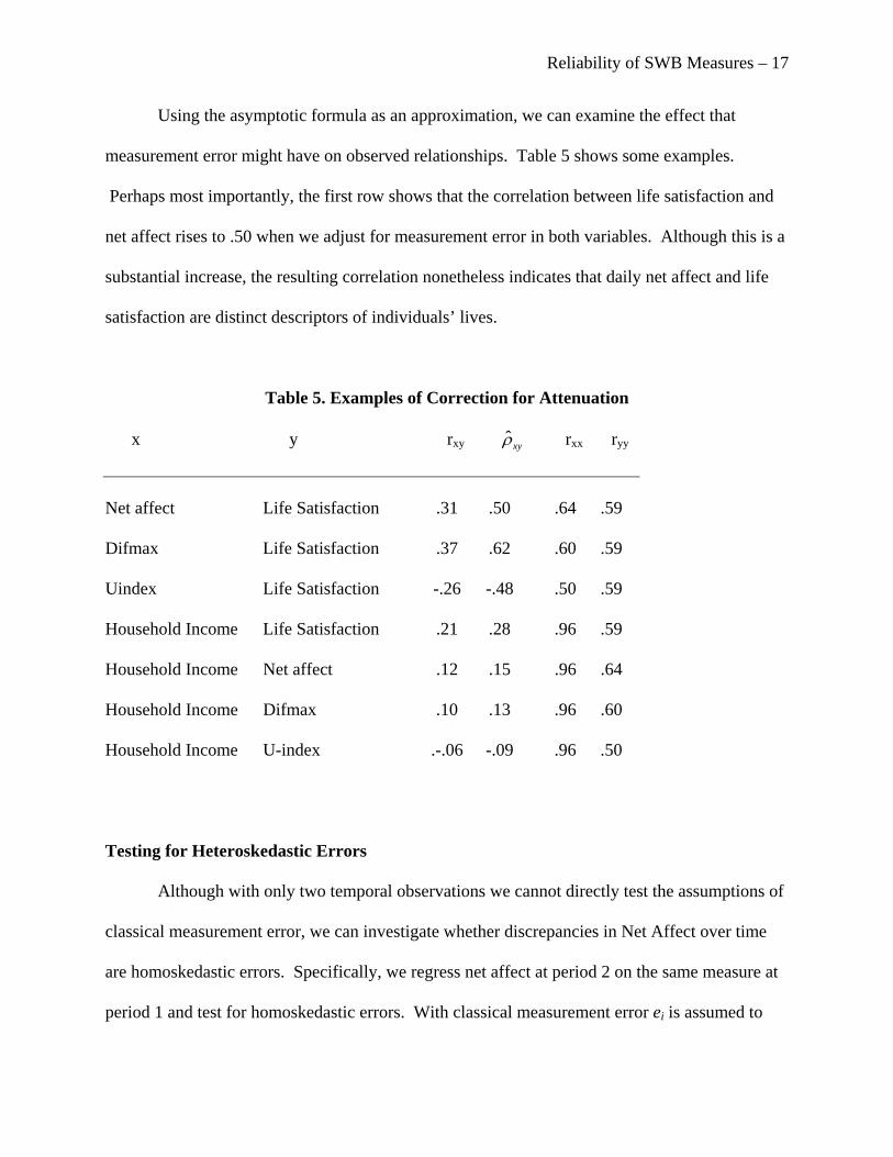
Using the asymptotic formula as an approximation, we can examine the effect that

measurement error might have on observed relationships. Table 5 shows some examples.

Perhap and

is is a

for Attenuation

x y rxy

s most importantly, the first row shows that the correlation between life satisfaction

net affect rises to .50 when we adjust for measurement error in both variables. Although th

substantial increase, the resulting correlation nonetheless indicates that daily net affect and life

satisfaction are distinct descriptors of individuals’ lives.

Table 5. Examples of Correction

ρ̂xy rxx ryy

.50

Difmax Life Satisfaction .37 .62 .60 .59

Testing for Heteroskedastic Errors

Although with only two temporal observations we cannot directly test the assumptions of

vestigate whether discrepancies in Net Affect over time

are hom

Net affect Life Satisfaction .31 .64 .59

Uindex Life Satisfaction -.26 -.48 .50 .59

Household Income Life Satisfaction .21 .28 .96 .59

Household Income Net affect .12 .15 .96 .64

Household Income Difmax .10 .13 .96 .60

Household Income U-index .-.06 -.09 .96 .50

classical measurement error, we can in

oskedastic errors. Specifically, we regress net affect at period 2 on the same measure at

period 1 and test for homoskedastic errors. With classical measurement error ei is assumed to


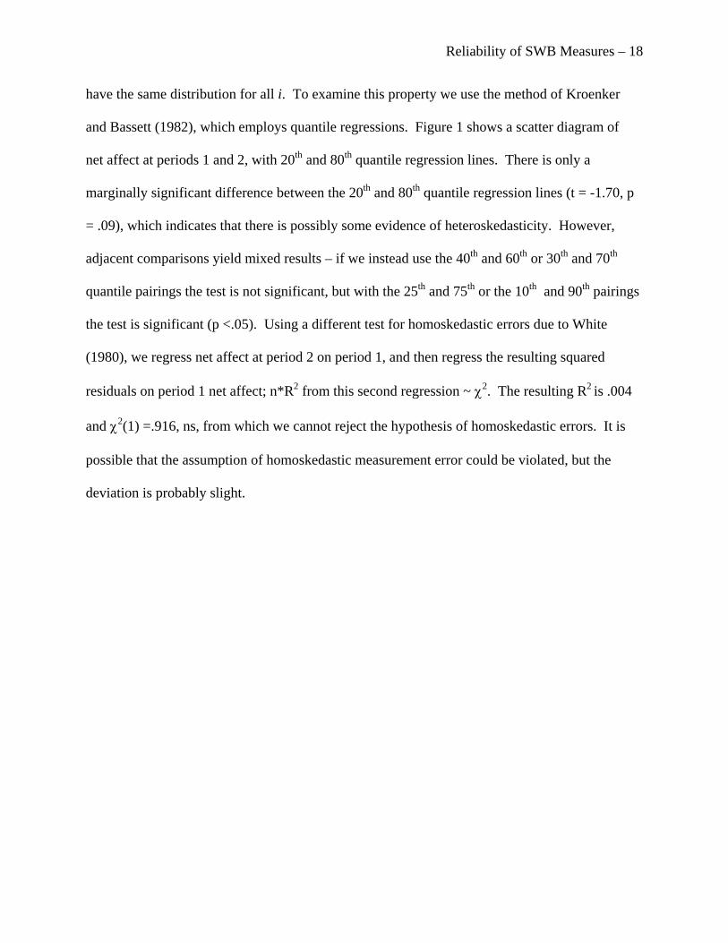
have the same distribution for all i. To examine this property we use the method of Kroenker

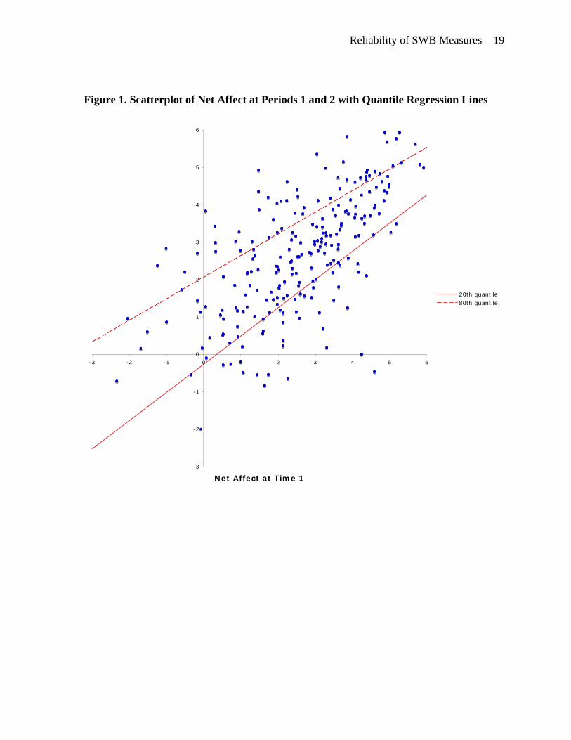
and Bassett (1982), which employs quantile regressions. Figure 1 shows a scatter diagram of

net affect at periods 1 and 2, with 20th and 80th quantile regression lines. There is only a

marginally significant difference between the 20th and 80th quantile regression lines (t = -1.70, p

= .09), which indicates that there is possibly some evidence of heteroskedasticity. Howev

adjacent comparisons yield mixed results – if we instead use the 40th and 60th or 30th and 70th

quantile pairings the test is not significant, but with the 25th and 75th or the 10th and 90th pairin

the test is significant (p <.05). Using a different test for homoskedastic errors due to White

(1980), we regress net affect at period 2 on period 1, and then regress the resulting squared

residuals on period 1 net affect; n*R2 from this second regression ~ χ2. The resulting R2 is .0

and χ2(1) =.916, ns, from which we cannot reject the hypothesis of homoskedastic errors. It

possible that the assumption of homoskedastic measurement error could be violated, but the

deviation is probably slight.

er,

gs

04

is


Figure 1. Scatterplot of Net Affect at Periods 1 and 2 with Quantile Regression Lines

-3

-2

-1

0

1

2

3

4

5

6

-3 -2 -1 0 1 2 3 4 5 6

Net Affect at Time 1

20th quantile80th quantile


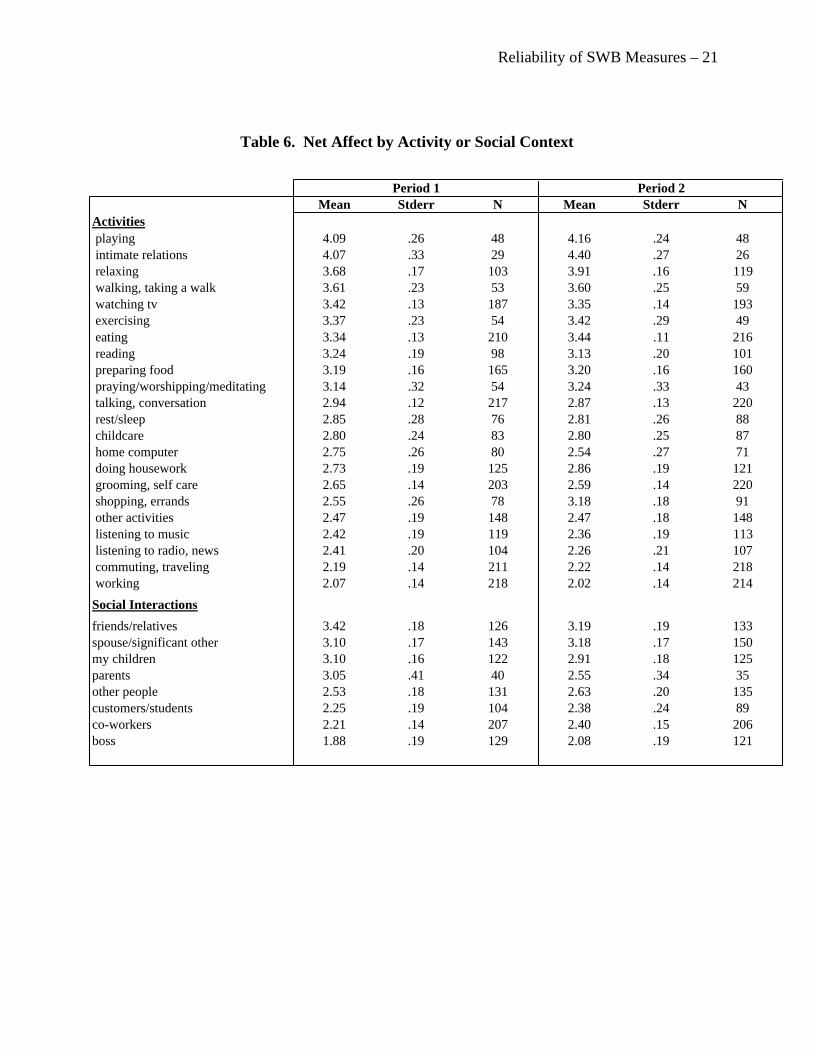
Reliability of Aggregate Activity Experience Ratings

The reliabilities we have computed thus far are defined at the level of the individual. For

many applications, however, the key issue is not the reliability of net affect for individuals, but

rather the reliability of average net affect across individuals engaged in various activities. The

question of reliability in this context is whether a given activity produces the same average

experience at different times. A simple test for this is to compute the mean values for each

activity for each time period and correlate the vectors across activities. Table 6 presents the mean

net affect for each day by activity and interaction partner. The two DRMs produce a remarkably

similar patterns of mean net affect across activities (r = .96, see Table 6 and Figure 2) and also of

relative frequency (r = .99, see third and sixth columns of Table 6).

_

jA


Table 6. Net Affect by Activity or Social Context

Mean Stderr N Mean Stderr NActivities playing 4.09 .26 48 4.16 .24 48 intimate relations 4.07 .33 29 4.40 .27 26 relaxing 3.68 .17 103 3.91 .16 119 walking, taking a walk 3.61 .23 53 3.60 .25 59 watching tv 3.42 .13 187 3.35 .14 193 exercising 3.37 .23 54 3.42 .29 49 eating 3.34 .13 210 3.44 .11 216 reading 3.24 .19 98 3.13 .20 101 preparing food 3.19 .16 165 3.20 .16 160 praying/worshipping/meditating 3.14 .32 54 3.24 .33 43 talking, conversation 2.94 .12 217 2.87 .13 220 rest/sleep 2.85 .28 76 2.81 .26 88 childcare 2.80 .24 83 2.80 .25 87 home computer 2.75 .26 80 2.54 .27 71 doing housework 2.73 .19 125 2.86 .19 121 grooming, self care 2.65 .14 203 2.59 .14 220 shopping, errands 2.55 .26 78 3.18 .18 91 other activities 2.47 .19 148 2.47 .18 148 listening to music 2.42 .19 119 2.36 .19 113 listening to radio, news 2.41 .20 104 2.26 .21 107 commuting, traveling 2.19 .14 211 2.22 .14 218 working 2.07 .14 218 2.02 .14 214Social Interactionsfriends/relatives 3.42 .18 126 3.19 .19 133spouse/significant other 3.10 .17 143 3.18 .17 150my children 3.10 .16 122 2.91 .18 125parents 3.05 .41 40 2.55 .34 35other people 2.53 .18 131 2.63 .20 135customers/students 2.25 .19 104 2.38 .24 89co-workers 2.21 .14 207 2.40 .15 206boss 1.88 .19 129 2.08 .19 121

Period 1 Period 2


Figure 2. Mean Net Affect for Activities by Session

0

0.5

1

1.5

2

2.5

3

3.5

4

4.5

5

0 0.5 1 1.5 2 2.5 3 3.5 4 4.5 5

Net Affect at Time 1

r = .96


Discussion

We analyzed the persistence of various subjective well-being questions over a two-week

period. We found that both overall life satisfaction measures and affective experience measures

derived from the DRM exhibited test-retest correlations in the range of .50-.70. While these

figures are lower than the reliability ratios typically found for education, income and many other

common micro economic variables, they are probably sufficiently high to support much of the

research that is currently being undertaken on subjective well-being, particularly in cases where

group means are being compared (e.g. rich vs poor, employed vs unemployed) and the benefits

of statistical aggregation apply.

It is perhaps surprising that measures intended to assess the general state of SWB over an

extended period (such as overall life satisfaction) should be no more reliable than measures of

affective experience on different days two weeks apart. One’s general level of life satisfaction

would be expected to change only very slowly over time, because so do most of its known

correlates (age, income, marital status, employment). A key factor behind this result is probably

the fact that answering a life satisfaction question explicitly invokes a nonsystematic review of

one’s life, which leaves such measures vulnerable to transient influences that draw attention to

arbitrary or incomplete information (e.g. one’s immediate mood, the weather). By contrast,

measures of affective experience from experience sampling or the DRM do not rely on such

cognitive appraisals, and have the benefit of aggregating over several episodes and adjectives,

They also have the disadvantage, however, that no two days (even if intentionally matched, as in

our study) are truly the same.


Another application of reliability estimates is to assist in the determination of appropriate

sample sizes for the measurement of various emotional experiences. In clinical trials, for

example, if SWB measures are one of the outcome variables of interest, reliabilities can be used

to help determine the sample size needed to detect an expected difference between groups.

Because the reliabilities are modest, the risk of incorrectly concluding that groups do not differ is

of particular concern. As we saw in our examples of correction for attenuation, the true strength

of relationships could easily be underestimated in the small samples that clinical research must

sometimes employ (e.g. with special populations). An alternate design approach to larger

samples of course would be reduce error by sampling the same people at different points in time.


References

Andrews, F. M. and Whithey, S. B. 1976. Social indicators of well being: Americans’ perception

of life quality. New York: Plenum,.

Angrist, J. and Krueger, A. B. 1999. “Empirical Strategies in Labor Economics,” Chapter 23 in

O. Ashenfelter and D. Card, eds., The Handbook of Labor Economics, Volume III, North

Holland.

Argyle, M. 1999. “Causes and correlates of happiness.” In D. Kahneman, E. Diener & N.

Schwarz (Eds.), Well Being: The Foundations of Hedonic Psychology. Russell Sage

Foundation.

Belli, R. 1998. “The structure of autobiographical memory and the event history calendar:

Potential improvements in the quality of retrospective reports in surveys” Memory, 6, 383.

Blanchflower, David and Andrew J. Oswald. 2004. “Well-being over time in Britain and the

United States.” Journal of Public Economics. 88, 1359-1386.

Bound, John, Charles C. Brown, Nancy Mathiowetz. 2001. “Measurement Error in Survey

Data." In Handbook of Econometrics, edited by E.E. Learner and J.J. Heckman. Pp.

3705-3843. New York: North Holland Publishing.

Csikszentmihalyi M, Larson R. 1987. “Validity and reliability of the Experience-Sampling

Method.” Journal of Nervous and Mental Disease, Sep;175(9):526-36.

Diener, E., RA Emmons, RJ Larsen, S Griffin. 1985. “The Satisfaction With Life Scale.”

Journal of Personality Assessment. 49, 1.

http://www.ncbi.nlm.nih.gov/entrez/query.fcgi?db=pubmed&cmd=Search&itool=pubmed_Citation&term=%22Csikszentmihalyi+M%22%5BAuthor%5D

http://www.ncbi.nlm.nih.gov/entrez/query.fcgi?db=pubmed&cmd=Search&itool=pubmed_Citation&term=%22Larson+R%22%5BAuthor%5D


Easterlin, Richard A. (1995) “Will Raising the Incomes of All Increase the Happiness of All?”

Journal of Economic Behavior and Organization, 27(1), (June), pp. 35-48.

Eid, M., & Diener, E. (2004). “Global judgments of subjective well-being: Situational variability

and long-term stability.” Social Indicators Research, 65, 245-277.

Ferring, D., S.-H. Filipp and K. Schmidt: 1996, The “Skala zur Lebensbewertung:” Scale

construction and findings on reliability, stability, and validity, Zeitschrift für

Differentielle und Diagnostische Psychologie 17, pp. 141–153.

Frey, B. and A. Stutzer. 2002. “What Can Economists Learn from Happiness Research?”

Journal of Economic Literature. 40, No. 2, June 2002

Kahneman, D., Diener, E. and Schwarz, N. 1999. Well Being: The foundations of hedonic

psychology. NY: Russell Sage.

Kahneman, Daniel and Alan B. Krueger. 2006. “Developments in the Measurement of

Subjective Well-Being.” Journal of Economic Perspectives. 20, 3–24.

Kahneman, D., Krueger, A., Schkade, D., Schwarz, N. and Stone, A. 2006. “Would you be

happier if you were richer? A focusing illusion.” Science, 312, 1908-1910.

Kahneman, D., Krueger, A., Schkade, D., Schwarz, N. and Stone, A. 2004. “A survey method

for characterizing daily life experience: The Day Reconstruction Method (DRM).”

Science, 306, 1776-1780.

Kammann, R. and Flett, R. 1983. Affectometer 2. A scale to measure current level of happiness.

Australian Journal of Psychology, 35, 259-265.


Kammann, R. 1984. “The analysis and measurement of happiness sense of well-being.” Social

Indicators Research, 15, 91.

Kroenker, Roger, and Bassett, Gilbert. 1982. “Robust tests for heteroscedasticity based on

quantile regressions.” Econometrica, 50, 43-62.

Layard, Richard. 2005. Happiness: Lessons from a New Science,. Penguin Books: London.

Lyubomirsky, S. and Lepper, H. S. 1999. “A measure of subjective happiness: Preliminary

Reliability and construct validation.” Social Indicators Research 46: 137–155.

Lyubomirsky, S., Sheldon, K. and Schkade, D. 2005. “Pursuing happiness: The architecture of

sustainable change.” Review of General Psychology, 9, 111-131.

Nunnally, J. C. 1978. Psychometric theory. 2nd edition. New York: McGraw-Hill, pp236-237.

William Pavot and Ed Diener. 1993. “Review of the Satisfaction With Life Scale.”

Psychological Assessment, 5, 164-172.

Pavot, W., E. Diener, C. R. Colvin and E. Sandvik. 1991. “Further validation of the Satisfaction

with Life Scale: Evidence for the cross-method convergence of well-being measures.”

Journal of Personality Assessment 49, 71–75.

Robinson, M. D. and Clore, G. L. 2002. “Belief and feeling: Evidence for an accessibility model

of emotional self-reports.” Psychological Bulletin, 128, 934.

Schwarz, Norbert. 1987. Stimmung als Information: Untersuchungen zum Einfluß von Stimmungen

auf die Bewertung des eigenen Lebens. Heidelberg: Springer Verlag.


Steptoe, A., J. Wardle and M. Marmot. 2005. “Positive Affect and health-related

neuroendocrine, cardiovascular, and inflammatory processes.” PNAS, 102, no. 18, 6508-

12.

Stone, A. A., Schwartz, J. E., Schwarz, N., Schkade, D., Krueger, A. and Kahneman, D. 2006.

“A population approach to the study of emotion: Diurnal rhythms of a working day

examined with the Day Reconstruction Method (DRM).” Emotion, 6, 139-149.

Stone, A. A., Shiffman, S. S., DeVries, M. W. 1999. “Ecological momentary assessment.” In

Well-Being: The Foundations of Hedonic Psychology, D. Kahneman, E. Diener, N.

Schwarz, Eds. (Russell-Sage, New York, pp. 61–84.

White, H. 1980, “A heteroskedasticity-consistent covariance matrix estimator and�a direct test

for heteroskedasticity.” Econometrica. 48, 817-838.

The Reliability of Subjective Well-Being Measures · display a serial correlation of about 0.60...

Documents

Transcript of The Reliability of Subjective Well-Being Measures · display a serial correlation of about 0.60...