The Relevance of Political Stability on FDI: A VARAnalysis and ARDL Models for Selected Small,Developed, and Instability Threatened Economies

Kurečić, Petar; Kokotović, Filip

Source / Izvornik: Economies, 2017, 5, 1 - 18

Journal article, Published versionRad u časopisu, Objavljena verzija rada (izdavačev PDF)

https://doi.org/10.3390/economies5030022

Permanent link / Trajna poveznica: https://urn.nsk.hr/urn:nbn:hr:122:719892

Rights / Prava: In copyright

Download date / Datum preuzimanja: 2022-03-22

Repository / Repozitorij:

University North Digital Repository

economies

Article

The Relevance of Political Stability on FDI: A VARAnalysis and ARDL Models for Selected Small,Developed, and Instability Threatened Economies

Petar Kurecic 1,* and Filip Kokotovic 2

1 Business and Economics Department, University North, Koprivnica 48000, Croatia2 University College of International Relations and Diplomacy Dag Hammarskjöld, Zagreb 10000, Croatia;

filip.kokotovic@hotmail.com* Correspondence: pkurecic@unin.hr; Tel.: +38-598-980-8577

Academic Editor: Eric RougierReceived: 27 April 2017; Accepted: 13 June 2017; Published: 22 June 2017

Abstract: This paper studies the relevance of political stability on foreign direct investment (FDI)and the relevance of FDI on economic growth, in three panels. The first panel contains 11 very smalleconomies; the second contains five well-developed and politically stable economies with highlypositive FDI net inflows, while the third is a panel with economies that are prone to political violenceor targeted by the terrorist attacks. We employ a Granger causality test and implement a vectorautoregressive (VAR) framework within the panel setting. In order to test the sensitivity of the resultsand avoid robust errors, we employ an ARDL model for each of the countries within every panel.Based upon our results, we conclude that there is a long-term relationship between political stabilityand FDI for the panel of small economies, while we find no empiric evidence of such a relationshipfor both panels of larger and more developed economies. Similarly to the original hypothesis ofLucas (1990), we find that FDI outflows tend to go towards politically less stable countries. On theother hand, the empiric methodology employed did not find such conclusive evidence in the panelsof politically more developed countries or in the small economies that this paper observes.

Keywords: political stability; VAR analysis; Granger causality test; investor confidence; ARDL analysis

JEL Classification: C32; C33; O1; F21

1. Introduction

Foreign direct investment (FDI) is considered an important motivator of economic growth.There are various studies that address the issue of the relevance of FDI to economic growth,comprising numerous other macroeconomic variables. As such, this study aims to fill the literaturegap in understanding the psychological factor of macroeconomic dynamics as becoming increasinglyimportant in determining the key components of economic growth. The approaches to identifyingkey trends are increasingly interdisciplinary, while intuitive claims and policy discussions should beaccompanied by adequate quantitative analysis and empirical proof. This was especially obviousduring the time of the 2008 crisis, as noted by Krugman (2009), who claims that investor confidenceand their perceptions or prejudice currently are the key economic elements. In these times, perhaps,the issues of perception and investor’s confidence are becoming increasingly important in maintainingstable economic growth. Perhaps a key element to the issue of public awareness is the media coverage,as indicated in several studies that point out the so-called “CNN effect”.

Economies 2017, 5, 22; doi:10.3390/economies5030022 www.mdpi.com/journal/economies

Economies 2017, 5, 22 2 of 21

The “CNN effect”1 is perhaps far more important in the sphere of political science, sociology andjournalism, but as this study will attempt to assess, it may have a profound effect on the economicsituation (Gilboa 2005; Robinson 2005; Livingston and Eachus 1995). Instead, media coverage andpublic awareness of episodes of political violence is far more significant in larger countries wherethere is global public interest in the events unfolding. Thakur (2006) (p. 55) emphasizes that theUnited Nations officials attempted to negotiate with media representatives to further their coverageof episodes of political violence to make the American public opinion more inclined to foreignintervention. The importance of media coverage is not contained to the sphere of high politicsand conflict management; it also may have significant impact on key economic indicators such asFDI. Thus, it is possible to approach the issue from two completely different initial hypotheses. Onepossible hypothesis is that there is a more profound effect of episodes of political violence in largercountries on economic growth and FDI. On the contrary, very small countries are not in the mediaspotlight. An alternative hypothesis may be that investors are not so much concerned with politicalstability in large countries and that political stability is far more relevant in small economies, whereinvestors require political stability as an initial condition to consider such areas as the targets forinvestment. In this paper, we aim to consider both hypotheses, empirically and theoretically, andprovide conclusions on which hypothesis is substantiated with more empiric evidence. Thus, the paperaims to understand the impact of political stability on FDI, while also engaging in a discussion on theimpact of FDI on economic growth itself. By considering both of these aspects and by implementingseveral relevant quantitative approaches, we aim to understand the relevance of these factors foreconomic growth and find relevant policy implications. As will be emphasized in the literature review,we find that many studies are robust in considering panels of countries and cross-section data that donot take into account the economic development of the country, nor its political climate. In order to doso, the introduction will be followed by a short review of the existing literature. It will be followedby a discussion on the methodological approach of the paper. Furthermore, the paper will provide atheoretical discussion and summary of the results obtained from the empiric approach. Finally, thepaper will provide relevant policy recommendations based upon the results.

2. Literature Review

Many researchers in finance and economics try to find the factors that affect FDI. An importantelement that needs to be mentioned is that, aside from the direct impact of FDI, there can also be amultiplier effect on economic growth. As emphasized by Ray (2012), FDI causes increased employmentand productivity, enhanced technological improvements and boosts in exports. It is therefore importantto notice that the empirical assessment of FDI can only take note of the direct (net) impact on economicgrowth, while it isn’t fully able to capture the “spillover” or multiplier impact on the economy.Regardless, there have been numerous empiric research papers that analyze the impact of investmentson economic growth.

For example, Lucas (1990) argues that only political risk is an important factor in limiting capitalflows. Investments in many developing countries are exposed to large political risks, so FDI inflows arelarge for politically unstable countries. For the same reason, FDI outflows are large for politically stablecountries to invest in countries with large political risks (Haksoon 2010, p. 59). From all sources that wehave explored, Almfraji and Almsafir (2014) did the most comprehensive and systematized literaturereview on FDI effect on the economic growth from 1994 to 2012 that we came across. This review paperhas concluded that the majority of papers suggest that there is a positive relationship between FDI and

1 Simply stated, the CNN effect states that there is a strong connection between the news that is covered and policy-making(Gilboa 2005). This can be extended to the sphere of global economics, despite the primary field of the CNN effect beingjournalism and political science, where the impact of TV coverage on policy-making is discussed. The way we attemptto do so is through understanding whether negative coverage of political events decreases investor confidence into thesecountries and thus, investments.

Economies 2017, 5, 22 3 of 21

economic growth, although they emphasize that there are instances where papers concluded that therewas no, or even a negative, impact (Almfraji and Almsafir 2014). Our own literature review has foundsimilar discrepancies in the existing literature.

2.1. The Comparative Studies Explored

Kholdy (1995) has examined ten East Asian countries and by implementing Granger causalitytests determined that there is no causality between FDI and productivity, though this may bedue to the nature of Granger causality tests, as later discussed in the methodology section.Balasubramanyam et al. (1996) concluded that FDI inflows are far more significant for countries thatfocus on export, rather than those who have a negative trade balance. In her study of foreign directinvestments (FDI) in three regions of the South (South-East Asia, Sub-Saharan Africa, and CentralAmerica), McMillan (1999) studied the various patterns of FDI in the following countries: Thailand andthe Philippines; Cote D’Ivoire and Ghana; Costa Rica and Guatemala). The author used MultivariateGranger Causality Tests on each country. The principal result of the comparisons is that the domesticcontext of FDI generates identifiable patterns of development outcomes. However, FDI is not theprimary causal agent in development outcomes. The results support the contention that FDI wasdrawn in by a strong bargaining context, but that it is not itself a particularly strong determinant ofdomestic economic and political outcomes. Elkomy et al. (2016) have conducted their own empiricanalysis upon 61 transition and developing countries for the period 1989 to 2013. The paper finds thatthere is no critical threshold of human capital requirement in order for the spillover effect of FDI tobe achieved and further finds that domestic investments is a much more significant driving force indemocratic countries (Elkomy et al. 2016).

The study of Bacic et al. (2004) focuses on the impact of FDI on economic growth in eleventransitional countries. Their conclusion is that there is a statistically significant positive impact ofFDI inflows in small countries, such as Slovenia, Slovakia and Lithuania, yet the impact was farmore pronounced in more developed countries (Bacic et al. 2004). Similarly, Asteriou et al. (2005)focus on the impact of FDI on economic growth of ten European transition countries. Their mainconclusion is the existence of a positive correlation between FDI and economic growth, yet they alsodetect a negative correlation between portfolio investments and economic growth (Asteriou et al. 2005).Brada et al. (2005) studied the effects of transition and political instability on foreign direct investmentin ECE and found the fact that they were countries in transition enabled those increased FDI inflowsin comparison with West European countries. This somewhat contrasts the findings of Elkomy et al.(2016), who find that there is no impact of FDI on economic growth in transitional countries.

Haksoon (2010) in his study of the influence of political stability on FDI suggests two hypotheses,with the first being that FDI inflows generally flow towards countries that suffer from instances ofpolitical instability, while FDI inflows tend to flow from politically stable countries. Haksoon (2010)second hypothesis is that, after adjusting for macroeconomic factors, the inwards performance ofFDI is high for countries that suffer from instances of political instability. He managed to confirmboth hypotheses with an emphasis that this conforms to the findings of Lucas (1990). These findingssuggest that there is an increased level of FDI towards countries that have a higher level of politicalcorruption and suffer from instances of political instability (Haksoon 2010). A pooled ordinary leastsquares (OLS) with robust standard errors for the panel data using robust (cluster) covariance matrixas in Wooldridge (2002), was performed first with several other quantitative method analysis toconfirm the hypotheses. Khan and Mashque (2013) determine a negative and significant relationshipbetween political risk and FDI, accounting for 94 countries over a span of 24 years from 1986–2009.They conclude that most of the political risk indicators have a negative relationship with FDI for theworld as a whole and the high-income countries but the relationship was the strongest for the uppermiddle-income countries.

Iamsiraroj and Doucouliagos (2015) study the success of economic growth in attracting FDI.Meta-regression analysis is applied to 946 estimates from 140 empirical studies. The authors show

Economies 2017, 5, 22 4 of 21

that there is a robust positive correlation between growth and FDI. Significantly, larger correlations areestablished for single country case studies than with cross-country analysis. Cicak and Soric (2015)study the impact of FDI inflows on economic growth in Croatia and other selected transition economiesby implementing a VAR approach. The key conclusion of the paper is that there is evidence of Grangercausality going from FDI towards economic growth (Cicak and Soric 2015). Another significant aspectis that Cicak and Soric (2015) determine that, based on their results for Latvia and Slovenia, investorconfidence is increased in case of a more stable macroeconomic environment.

Mehrara et al. (2010) employed a panel data approach to a sample of 57 developing countries inwhich they determined that there is a short-run causality from FDI net inflows and exports to GDP.Several studies mention the relevance of political factors to FDI, such as Büthe and Milner (2008) whostart with a standard economic model as follows:

FDI(i,t) = α + γ1(Market Size)i, (t−1) + γ2(Econ. Development)i, (t−1)+

γ3(GDP growth)i, (t−1) + δ1 + εi,t,(1)

where FDI is the natural logarithm of the values of foreign direct investment, market size is the naturallogarithm of the values of population, Econ. Development is the log of per capita GDP; GDP growthproxies economic growth; δ1 is a country fixed dummy variable, and α is the constant and ε is the errorterm.

To this simple model, they added several political variables, notably bilateral investment treaties,GATT/WTO membership, domestic political constraints and political instability (Büthe and Milner2008, p. 750). They conclude that adding each variable improves the explanatory value of the modeland it is interesting to note that they find a slightly, but statistically significant negative effect ofpolitical instability on FDI (Büthe and Milner 2008). Bisson (2011) (Bisson) employed an OLS regressionto determine that the relevance of several variables used as proxies for political instability werestatistically significant to a cross-section group of 45 selected developing countries. Jadhav (2012)conducted a panel regression approach to the BRICS countries from 2000–2009, using the followingempiric strategy:

FDIit = α + β1MSit + β2NRAit + θ(Institutional Variables)it+

µ(Policy Variable)i,t + ϕ(Political Risk Variable)it + εi,t,(2)

where FDI is foreign direct investment, MS measures market size, NRA is the Natural resourceavailability, θ measures Corruption, Rule of Law, Voice and Accountability, µ accounts for the Inflationrate and the Trade to-GDP ratio, ϕ accounts for Political Stability and No Violence, GovernmentEffectiveness, Regulatory Quality, with the constant α, while the error term is represented by ε.

By using such an empiric strategy, Jadhav (2012) (pp. 11–12) failed to obtain statistically significantresults, even at the 10% level of significance, for the variables that concern political stability and ruleof law, while voice and accountability was statistically significantly negatively associated with FDI.Busse and Hefeker (2005) implemented a panel GMM approach to a series of variables that measurepolitical stability and the quality of government and concluded that government stability, the absenceof internal conflict and ethnic tensions, basic democratic rights and ensuring law and order have astatistically significant effect on FDI. As emphasized by her detailed literature review, Pandya (2016)finds that many countries have become more open to FDI through an increase in the volume of tradeand trade agreements, deregulation, as well as investment incentives.

2.2. Selected Studies of Single Economies Explored

Onwuka and Zoral (2009) studied the long-term relationship between FDI and import growth inTurkey. The authors include both the traditional import demand function with the inclusion of FDI,as well as an ARDL and FMOLS approach to confirm their hypothesis and avoid the possibility of

Economies 2017, 5, 22 5 of 21

robust errors. Akande and Oluyomi (2010) explored the relevance and application of the theoreticalprescriptions of the Two-Gap model to the Nigerian economic growth situation from 1970 to 2007.A co-integration test confirmed that a long-running relationship exists among the variables, giving anindication that they have the tendency to reach equilibrium in the long run.

Al-Eitan (2013) studied the influence of FDI on economic growth in Jordan, from 1996 to 2010,using several quantitative methods such as VAR models and Granger causality. Based on the analysis,the results showed that Jordan economic risk, the price of stock market sectors and two of themacroeconomic variables (inflation and GDP) significantly caused inward FDI in Jordan. Aga (2014)studies the impact of FDI on economic growth on the example of Turkey for the 1980–2012 periods.The paper utilizes the Johansen co-integration test whereby it finds no co-integration and long runrelationship between variables.

2.3. Summary of Literature Review and Implications

As was previously pointed out in Almfraji and Almsafir (2014), there are a number of significantdiscrepancies in the existing literature. Most significantly, there is no clear consensus on whether thereis a positive impact of FDI on economic growth. Furthermore, there is a lack of consensus on whetheror not the relationship is significant in only the short-term or whether there is a long-term relationshipbetween the two variables. For the purpose of this paper, the results of two papers have perhaps themost significant implications. Primarily, this is the finding of Haksoon (2010) that complies with thetheory of Lucas (1990) that there is an increased level of FDI inflows into countries that are impacted bypolitical corruption and instability. On the other hand, Jadhav (2012) finds no evidence of any impactof political stability and rule of law on FDI. All of these findings will be considered (Büthe and Milner2008; Jadhav 2012; and Cicak and Soric 2015) and discussed upon evaluating our empiric results. Priorto conducting our empiric analysis, we discuss in detail our methodological approach.

3. Methodology

The data employed for the empiric analysis was extracted from the World Bank (2016) database,the values of GDP in current dollars and the net inflow of FDI in current dollars and for the exportof goods and services in current dollars for the period of 1996–2014. The data was then corrected forinflation using the GDP deflator, also acquired from the World Bank (2016) database.2 The data was alsoextracted for population of each country, as well as the arable land available, measured in thousandsof hectares. The variable that concerns political stability was obtained from the dataset constructed byKaufmann et al. (2010). Their index ranges from −2.5 to +2.5 for the considered variables—politicalstability and the absence of violence/terrorism. Higher values of this index indicate a higher level ofpolitical stability, while lower levels indicate a diminished level of political stability and more frequentoccurrences of violence, as well as terrorist attacks. We consider three different panels, a panel of smalleconomies, a panel of developed western economies and a panel of economies that are known forissues regarding political violence or are frequently targeted by terrorists. Exact specifications of thepanels are available in the Appendix A, while the panels are further referred to as panel A for thepanel of small economies, panel B for the panel of developed economies and panel C for the panel ofcountries that have issues regarding political violence and terrorist attacks, respectively. A significantbenefit of such a panel specification was that, in the observed period, the FDI inflow values for themajority of the considered countries were positive. This allows the paper to focus on substantialissues regarding the effect of political stability on FDI inflows without resorting to methods sometimesconsidered controversial.3 The countries were divided into three separate panels, as specified in

2 Using the formula GDP t × GDP deflator base year/GDP deflator t where the base year was the value of the GDP deflator forthe last year where the data was available—in most cases, 2014 and t are the years for which the GDP data was available.

3 There are two possible solutions when considering negative FDI inflows. Not using logged versions of the variablesprobably results in heteroscedasticity issues, amongst others. Thus, two solutions are possible: considering the negative

Economies 2017, 5, 22 6 of 21

Table A1 in the Appendix A. The states that were put into the three different panels (small economies,large developed economies, and economies that were threatened by terrorist attacks or instances ofpolitical instability) were chosen arbitrarily, albeit with certain prerequisites. Of the 11 small economiesthat were studied, eight were small island economies (six from the Caribbean), and three were smallAfrican economies.

Developed economies that were studied represent some of the most developed economies, andat the same time all of them are among the 15 largest economies of the world, being members of theTriad (North America-the EU-Asia-Pacific Rim region), as the core of the world economy, although itsrelative “weight” in the world economy is slowly declining. In 2014, Australia was the 12th economyof the world, Canada 11th, France 6th, United Kingdom 5th, and the United States 1st. The economiesof the countries that have issues regarding political violence and terrorist attacks were studied throughfour examples that were placed in panel C: Mexico (due to the anti-drug warfare mostly), Israel, theRussian Federation, and Turkey. The panels are therefore clearly separated by size—panel A consistsof small economies in comparison to B and C.

The panels also are differentiated based on political stability that is essential to FDI inflows,although the literature review does not provide conclusive evidence on how political stability willimpact our final results. All of the countries that are included in panel C have consistently negativevalues for political stability based on the index created by Kaufmann et al. (2010) and this is theprimary determinant of this panel. As many papers have previously stated, it is slightly difficult todetermine the smallness of the economy, but all of the countries that are used in panel A have eithercomparatively small populations in regards to panels B and C, as well as economic growth that seemsinsignificant when compared to the values in panels B and C. A full list of these countries is presentedin the Appendix A.

Before considering further quantitative methods of analysis, several unit root tests will be usedto test for the presence of unit root. This will be conducted by using the tests originally proposedby Levin et al. (2002), as well as Im et al. (2003), and augmented versions of the test proposed byPhillips and Perron (1988) and Dickey and Fuller (1979). All of these tests are conducted against thenull hypothesis of a unit root present and are conducted by an autoregressive procedure based upon asuitable number of lags. The number of lags is determined by the information criterion proposed bySchwarz (1978). Selected summary statistics for all of the variables, in level and without any statisticaltransformation, are available in the Appendix A, as Table A2. In our empiric approach, the variablesthat measure economic growth, exports, as well as FDI will always be considered in the form of theirnatural logarithm after we have corrected the values for inflation. After conducting the unit root teststhe following three-step empiric strategy is considered.

3.1. Panel Model

Following the results of the conducted panel root test, we will estimate a test for causality betweenFDI, political stability and absence of violence/terrorism and GDP for each of the panels, by usingthe test initially proposed by Granger (1969). The Granger causality test is conducted by running abivariate regression, which displays whether adding lagged versions of a variable helps explain thebehavior of the independent variable. Therefore, the test will be conducted in the following form:

Yi,t= α0,i+α1,1Yi,t−1+ . . . + αl,iYl, t−l+β1,iXi, t−1+ . . . + βl,iXl,−l + . . . + εi,t, (3.1)

Xi,t= α0,i+α1,1Xi,t−1+ . . . + αl,iXl, t−l+β1,iYi, t−1+ . . . + βl,iYl,−l + . . . + εi,t, (3.2)

values as NA-s or adding an arbitrary constant. As we find, the first approach unacceptable and accept that the second is notconsidered adequate universally, the suggested panel specification seems like the best approach to focus on the substantialissues of this paper.

Economies 2017, 5, 22 7 of 21

where X, Y are the variables observed in the regression,4 α0,i is the constant, εi,t : is the error term andα1..l and β1..l are the coefficients.

The Granger causality test is then conducted by estimating the Wald test for the significance ofthe joint hypothesis:

β1 = β2 = . . . = βl = 0. (3.3)

In accordance with Granger (1969) initial methodology, the null hypothesis is therefore thatthere is no Granger causality between the variables. Rejection of the null hypothesis at the observedsignificance levels implies a statistically significant causal relationship.

3.2. Vector Auto Regression

Following the Granger causality test, we will conduct a Vector auto regression (VAR) model.The model is in detail specified in Equation (4):

FDIt = α0 + α1FDIt−1 + . . . + α1,2FDIt−n + α2Yt−1 + . . . + α2,1Yt−n + α3POLt−1 + . . .+

α3,1POLt−n + α4Ct + εt,1,(4.1)

POLt = β0 + β1FDIt−1 + . . . + β1,2FDIt−n + β2Yt−1 + . . . + β2,1Yt−n + β3POLt−1 + . . .+

β3,1POLt−n + β4Ct + εt,2,(4.2)

Yt = γ0 + γ1FDIt−1 + . . . + γ1,2FDIt−n + γ2Yt−1 + . . . + γ2,1Yt−n + γ3POLt−1 + . . .+

γ3,1POLt−n + γ4Ct + εt,3,(4.3)

where FDI is the log of foreign direct investment, Y is the log of real GDP, POL is the variablethat accounts for political stability and absence of violence/terrorism, C is the exogenous controlvariable; α1..4, β1..4, γ1..4 are the coefficients, α0, β0, γ0 are the constants, while ε1..3 represents the vectorof innovation.

This model will provide us with a more detailed understanding of the variables that are relevantto the increase of FDI. Primarily the interest of this paper is the impact of GDP and political stabilityand absence of violence/terrorism. We consider the variables Foreign Direct Investment (FDI), GrossDomestic Product (GDP) and political stability (POL) endogenous to the model. The remainingvariable serves as a control variable that increases the explanatory value of the model. These potentialcontrol variables are the logged values of exports of goods and services (Exp), logged values of totalpopulation in thousands (Pop) and logged values of arable land in hectares (Land). The abbreviationsin the parenthesis will be used in conducting all further aspects of our empiric methodology. One ofthese three variables will be selected based upon stepwise regression, through the value of the teststatistic, in order to maximize the explanatory value of the model. We consider that all of thesevariables may have a statistically significant impact on FDI inflow, yet they are only control variablesand will therefore not be discussed in detail, as they are not the primary focus of this study. This VARis conducted by using OLS on the pooled data. The VAR framework is used primarily to understandthe impulse response of each of the selected panels and further study will be conducted on each of theindividual countries to test the relevance of any hypothesis gathered from both the Granger causalitytest and the VAR model. The lag length for each of the VAR models will be determined using theinformation criterion proposed by Akaike (1974). The specification tests will consider whether there isserial correlation between the residuals based upon the LM test, which was constructed based uponthe research by Breusch (1978) and Godfrey (1978). They shall also determine whether the VAR modelsconform to the stability condition.

4 In the case of our model, we examine causality between three variables—FDI, GDP and political stability and absence ofviolence/terrorism.

Economies 2017, 5, 22 8 of 21

3.3. ARDL Models

In order to check the validity of our previous results and as an additional sensitivity check, we willconduct autoregressive distributed lag (ARDL) analysis, proposed initially by Pesaran and Shin (1999),on each of the countries. The ARDL method has several significant advantages, notably the fact thatwe can use different lag lengths of the dependent and independent variables. Perhaps the greatestadvantage of the ARDL approach is that it can be used on both I(0) and I(1) variables, while, forinstance, traditional co-integration processes require both variables to be I(1) and the majority ofstandard regression processes require stationarity. If any variable is determined to be I(2) or higher, theARDL method cannot and will not be employed. The presence of a unit root is tested by conductingtests proposed by Dickey and Fuller (1979) and by Kwiatkowski et al. (1992). These tests will allow usto determine whether the ARDL analysis may be used for all of the models.

After estimating the correct number of lags based upon the Akaike information criterion, wefirst implement tests to confirm heteroscedasticity initially proposed by Breusch and Pagan (1979),the absence of serial correlation based upon the LM test and the tests of stability of the parametersbased upon the work of Page (1954) and Barnard (1959) will be conducted, although they will notbe presented in the paper. Once the models are properly estimated, we implement the Bounds testdevised by Pesaran et al. (2001) in order to estimate whether there is a long-term relationship betweenthe variables. We estimate two models: in the first model GDP is the dependent variable, FDI theindependent variable, while in the second FDI is the dependent variable, and political stability is theindependent variable. If the results of the Bounds test suggest we can reject the null hypothesis, weestimate the long-term coefficients.

3.4. Methodological and Data Constraints

A significant constraint of using the Granger causality method or rather any method in a panelsetting is not taking into account possible robust errors. This is the reason why we chose to employan ARDL model for each of the countries within the panel. The panel selection is subject to researchbias and while the panels were not completely arbitrarily constructed, the method of selection maycause specification errors. Panel C is especially heterogeneous regarding numerous economic andpolitical traits of the countries considered in the panel. Aside from the previously identified issues,the Granger causality test suffers from other issues that warranted the use of multiple empiric tests.Maziarz (2015) emphasizes that both log transformations and modifications of variables to ensure theirstationarity may cause potential errors with Granger’s causality test. He further points out that thistest is completely dependent upon Granger’s definition of causality, which is why the largest numberof studies correctly reference this causality as “Granger-cause” (Maziarz 2015). Another problem thatis emphasized is that there may be a third variable that might Granger-cause both variables, but such acase may lead to a false causality result (Maziarz 2015).

A significant data constrain was that data for the political stability and absence ofviolence/terrorism error was only available for the period 1996–2014, excluding 1997, 1999 and2001.5 On the other hand, we believe that that the variable we use to proxy for political stabilityconstructed by Kaufmann et al. (2010) is perhaps the most objective assessment of political stability.Thus, we accept the limited period in order to obtain the desired results.

4. Discussion and Results

In adherence with the previously described methodology, we first employ a series of panel unitroot tests to determine whether there is a unit root present. Based upon our analysis of the previeweddata, we conclude that the test with constant and without trend is adequate. The only variable where

5 The data for the years 1997, 1999 and 2001 was generated by averaging the values of the values for t − 1 and t + 1, meaningthat for the year 1997 the average value of the index for 1996 and 1998 was calculated.

Economies 2017, 5, 22 9 of 21

a linear trend was included was for the variable political stability in panel C. In order to obtainthe statistically most adequate results, only variables where all four conducted tests reject the nullhypothesis of unit root presence at the 5% significance level are deemed stationary. As previouslymentioned, the number of lags was identified based upon the criterion proposed by Schwarz (1978).When the variable was not stationary in level, the value of the test statistic for the difference in whichthe variable was stationary is presented in Table 1.

Table 1. Unit root tests.

Variable Levin, Lin andChu t

Im, Pesaran andSchin W-stat

ADF-Fischer ChiSquare

PP-Fischer ChiSquare Conclusion

GDP

Panel A −5.796 ** (0.0000) −1.886 * (0.0297) 35.471 * (0.0346) 33.55 (0.0545) I(1)In first difference −9.604 ** (0.0000) −9.206 ** (0.0000) 125.55 ** (0.0000) 143.425 ** (0.0000)

Panel B 0.078 (0.5311) 3.215 (0.9993) 1.147 (0.9997) 0.9334 (0.9999) I(1)In first difference −8.158 ** (0.0000) −7.446 (0.0000) 67.342 (0.0000) 65.938 (0.0000)

Panel C −8.705 ** (0.0000) −12.653 ** (0.0000) 117.31 ** (0.0000) 108.929 ** (0.0000) I(0)

FDI

Panel A −5.421 ** (0.0000) −5.001 ** (0.0000) 63.3486 ** (0.0000) 72.883 ** (0.0000) I(0)Panel B −2.021 * (0.0216) −1.565 (0.0588) 15.54 (0.1136) 14.113 (0.1679) I(1)

In first difference −11.932 ** (0.0000) −12.618 ** (0.0000) 118.22 ** (0.0000) 107.06 ** (0.0000)Panel C −3.958 ** (0.0000) −4.647 ** (0.0000) 37.947 ** (0.0000) 43.809 ** (0.0000) I(0)

Exp

Panel A −3.175 ** (0.0007) −2.529 ** (0.0057) 42.838 ** (0.0049) 45.155 ** (0.0025) I(0)Panel B 0.7669 (0.7784) 3.112 (0.9991) 0.9644 (0.9999) 0.87092 (0.9999) I(1)

In first difference −9.961 ** (0.0000) −9.58 ** (0.0000) 89.2926 ** (0.0000) 116.361 ** (0.0000)Panel C −8.723 ** (0.0000) −7.386 ** (0.0000) 64.405 ** (0.0000) 57.447 ** (0.0000) I(0)

PolPanel A −2.9711 ** (0.0015) −2.7115 ** (0.0033) 41.521 ** (0.0071) 39.909 * (0.0111) I(0)Panel B −1.761 * (0.0391) −1.679 * (0.0466) 10.44 * (0.0336) 9.636 * (0.047) I(0)Panel C −5.0694 ** (0.0000) −2.692 ** (0.0036) 28.21 ** (0.0004) 271.71 ** (0.0000) I(0)

Pop

Panel A 0.0599 (0.5239) 1.0002 (0.8414) 22.141 (0.4515) 56.4981 ** (0.0001) I(2)In second difference −6.474 ** (0.0000) −5.566 ** (0.0000) 83.12 ** (0.0000) 48.604 ** (0.0000)

Panel B −0.3597 (0.3595) 4.557 (1.000) 3.796 (0.9561) 1.56 (0.9987) I(2)In second difference −9.787 ** (0.0000) −9.488 ** (0.0000) 91.967 ** (0.0000) 94.309 (0.0000)

Panel C −4.713 ** (0.0000) −3.217 ** (0.0006) 31.882 ** (0.0001) 65.426 ** (0.0000) I(0)

Land

Panel A 0.043 (0.5173) −0.501 (0.3081) 13.965 (0.6013) 13.598 (0.6287) I(1)In first difference −9.091 ** (0.0000) −10.813 ** (0.0000) 128.805 ** (0.0000) 129.657 (0.0000)

Panel B 1.67 (0.9525) 0.421 (0.6632) 11.43 (0.325) 14.137 (0.1668) I(1)In first difference

Panel C −1.537 (0.0621) 0.244 (0.5964) 11.154 (0.1931) 10.834 (0.2113) I(1)In first difference −6.416 ** (0.0000) −7.379 ** (0.0000) 60.041 ** (0.0000) 59.721 ** (0.0000)

Note: values in the parenthesis represent the p value. * and ** indicate statistical significance at the respected 0.05and 0.01 levels of significance.

For the variable political stability, we reject the presence of a unit root in all three panels.6

Regarding the other variables, GDP for panels A and B, FDI for panel B and export for panel B failedto reject the null hypothesis of a unit root present in level—but, in the first difference, they reject thenull hypothesis at the 1% significance level. We find that arable land rejects the null of unit root inthe first difference, while population in both panel A and panel B rejects the unit root null hypothesisin the second difference, while, in panel C, it is stationary in level. The remaining variables werealready stationary at a level with only the log transformations being applied. Furthermore, unlessexplicitly specified otherwise, the variables are always considered in the transformed form in whichthey rejected the null hypothesis of unit root presence. The results of the Granger causality test arepresented in Table 2.

6 This is also the only variable to which no log transformation, or any other statistical transformation, had been applied.

Economies 2017, 5, 22 10 of 21

Table 2. Granger causality test.

Null HypothesisTest Statistic Value

Number of LagsPanel A Panel B Panel C

Pol does not Granger cause FDI 4.656 ** (0.0114) 3.561 * (0.0764) 2.214 (0.1905) 2Pol does not Granger cause FDI 12.582 *** (0.0005) 2.252 (0.1483) 1.3 (0.4171) 1Pol does not Granger cause GDP 1.682 (0.1906) 0.197 (0.823) 0.418 (0.6759) 2Pol does not Granger cause GDP 0.066 (0.4747) 0.391 (0.5383) 0.093 (0.7669) 1FDI does not Granger cause POL 0.909 (0.4058) 1.141 (0.3429) 0.269 (0.7725) 2FDI does not Granger cause POL 1.13 (0.2897) 0.0396 (0.5383) 0.0029 (0.9582) 1FDI does not Granger cause GDP 0.202 (0.8171) 0.226 (0.7982) 1.659 (0.195) 2FDI does not Granger cause GDP 2.142 (0.1442) 0.294 (0.5888) 12.6812 *** (0.0005) 1GDP does not Granger cause FDI 6.394 *** (0.0019) 2.62 * (0.0764) 15.167 *** (0.000) 2GDP does not Granger cause FDI 8.065 *** (0.0048) 3.634 * (0.0586) 0.057 (0.811) 1GDP does not Granger cause POL 2.431 * (0.0924) 0.211 (0.812) 0.342 (0.7233) 2GDP does not Granger cause POL 0.514 (0.4747) 0.264 (0.6126) 0.114 (0.7434) 1

Note: values in the parenthesis represent the p value. *, ** and *** indicate statistical significance at the respected 0.1,0.05, and 0.01 levels of significance.

Granger panel causality tests, especially when preformed with as stacked tests, may be prone torobust errors as was previously mentioned in the methodological and data constrains. Therefore, anyconclusions based upon these results should be taken with caution. So far, it is possible to determinethat there is empiric evidence that political stability is more relevant in smaller economies wherewe determine that there is a unidirectional causal relationship going from political stability to FDI.The results for panel A also have the largest value of the test statistic in regards to higher valuesof GDP Granger causing an increase of FDI. This is a relatively intuitive conclusion as higher GDPvalues are often associated with economic growth that is accompanied by a pro-investment climateand favorable other macroeconomic indicators may increase investor confidence and thus increase FDI.In the remaining panels, we fail to determine any causal relationship between political stability witheither GDP or FDI at the 5% statistical significance level. As the result is only significant at the 10%significance level for panel B, we will discuss this issue further in the continuation of the paper afterconducting further tests. For panel B, we also find unidirectional Granger causality going from GDPto FDI, while, in this initial phase of testing, it is difficult to make a conclusive argument regardingpanel C.

We include higher numbers of lags7 and with that specification, we detect bidirectional causalitybetween FDI and GDP at three lags, but we find that the relationship is unidirectional going from GDPto FDI when using a higher number of lags. Similar to the situation regarding panel B, we will refrainfrom making any conclusions before conducting further tests. While the information criterion proposedby Schwarz indicates that one lag is optimal, the criterion proposed by Akaike (1974) suggests that twolags are optimal. These results suggest that the results obtained with two lags are the most accurate, asthey repeat at higher instances of lags, but at this point, it is not possible to confirm that the causalrelationship is unidirectional going from GDP to FDI. The extreme heterogeneity of the countries inthe panel also prevents us from confirming such a conclusion at this time.

4.1. VAR Model Approach

The second quantitative research method employed is a VAR approach, as specified in themethodological discussion. The VAR approach will primarily be used to identify the Cholesky impulseresponse in order to better understand the relationship between FDI and GDP; as well as politicalstability and FDI. While the conclusions from the Granger causality test are noted, they did not haveany impact on the specification of the VAR model. As the coefficient results are not being considered,

7 Test results for the panel C Granger causality test with three lags, as well as a short discussion about the results, are availablein the Appendix A.

Economies 2017, 5, 22 11 of 21

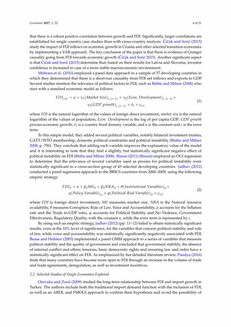
Table 3 provides brief summary statistics of the descriptive value and relevant statistics of the model,while specification tests are provided in the Appendix A. Briefly, it is possible to confirm that themodels are adequately specified as no root lies outside the unit circle. It is also possible to confirmthat the residuals are not serially correlated, with the values of the LM test for each model in theAppendix A.

Table 3. Summary of significant statistics for VAR models.

DependantVariable R-Squared Adjusted

R-SquaredS.E.

Equation F-Statistic AkaikeAIC

Number ofLags

Panel A

GDP 0.17 0.08 0.586 1.95 −2.153FDI 0.816 0.796 0.649 42.051 2.07

POL 0.944 0.939 0.195 161.34 −0.33

Panel B

GDP 0.801 0.581 0.029 3.63 −3.923FDI 0.778 0.532 0.424 3.158 1.422

POL 0.616 0.19 0.199 0.149 −0.671

Panel C

GDP 0.34 −0.04 0.271 4.683 −1.9371FDI 0.728 0.573 0.045 0.901 0.519

POL 0.916 0.868 0.079 19.105 −3.048

Aside from the endogenous variables, using stepwise regression, it was concluded that exportof goods and services would mostly enhance the explanatory value for each of the models, whilepopulation and arable land were deemed to have a statistically insignificant effect. Exports areconsidered exogenous for each model. For panel A, based upon the Akaike info criterion, three lagsshould be used and as with that lag length there is no evidence of models miss-specification, threelags were used. For panel B, four lags were suggested but at four lags, the model does not satisfy thestability condition. At three lags, the stability condition is satisfied and the LM test rejects the presenceof autocorrelation. For panel C, two lags were suggested. However, at such a specification, the modeldid not satisfy the stability condition. When the model was specified using one lag, it satisfied thestability condition and did not exhibit signs of autocorrelation.

The results from the Cholesky impulse function in Figure 1 regarding these two variables largelyconfirm the results obtained from the Granger causality tests. As we can see in panel A, the response isinitially highly positive, with a slightly declining trend in the long term. It should be noted that, forpanel B and panel C, 10 periods were used, while for panel A, 15 periods were used. The reason forthis arbitrary change is the fact that the authors wished to consider the response after 10 periods inpanel A to see whether the trend will continue to decline. Therefore, it is possible to conclude thatthere are significant differences between the Cholesky impulse response function to the introduction ofone standard deviation of political stability to FDI between panel A, and panels B and C. The responsefor panel B seems spurious, which is logical when taking into account that these are highly developedeconomies that are not likely to be affected by occasional terrorist attacks or isolated episodes ofpolitical violence. Taking into account the findings by the Granger causality test, it is possible toconfirm that a statistically significant consistent link between FDI and political stability for panelB does not exist. The response for panel C has the smallest initial response and it starts to declinestrongly after three periods until and seems to have a marginal impact at around 6 periods. The resultsseem to indicate that political stability is relevant to FDI both short-term and long-term in panel A,only relevant in the short-term for panel C, while it seems to have no statistically significant value forpanel B. It is once again possible to observe significant differences between the three panels in Figure 2,as in panel A the impact becomes negative after two periods and no longer becomes positive after that.

Economies 2017, 5, 22 12 of 21

Economies 2017, 5, 22  11 of 22 

 

The  second  quantitative  research method  employed  is  a VAR  approach,  as  specified  in  the 

methodological  discussion.  The VAR  approach will  primarily  be  used  to  identify  the Cholesky 

impulse response in order to better understand the relationship between FDI and GDP; as well as 

political stability and FDI. While the conclusions from the Granger causality test are noted, they did 

not have any impact on the specification of the VAR model. As the coefficient results are not being 

considered, Table 3 provides brief summary statistics of the descriptive value and relevant statistics 

of  the model, while  specification  tests  are provided  in  the Appendix A. Briefly,  it  is possible  to 

confirm  that  the models are adequately  specified as no  root  lies outside  the unit  circle.  It  is also 

possible to confirm that the residuals are not serially correlated, with the values of the LM test for 

each model in the Appendix A. 

Table 3. Summary of significant statistics for VAR models. 

Dependant 

Variable R‐Squared 

Adjusted 

R‐Squared 

S.E. 

Equation F‐Statistic 

Akaike 

AIC 

Number of 

Lags 

Panel A 

GDP  0.17  0.08  0.586  1.95  −2.15 

3 FDI  0.816  0.796  0.649  42.051  2.07 

POL  0.944  0.939  0.195  161.34  −0.33 

Panel B 

GDP  0.801  0.581  0.029  3.63  −3.92 

3 FDI  0.778  0.532  0.424  3.158  1.422 

POL  0.616  0.19  0.199  0.149  −0.671 

Panel C 

GDP  0.34  −0.04  0.271  4.683  −1.937 

1 FDI  0.728  0.573  0.045  0.901  0.519 

POL  0.916  0.868  0.079  19.105  −3.048 

Aside from the endogenous variables, using stepwise regression, it was concluded that export 

of goods and services would mostly enhance  the explanatory value for each of  the models, while 

population  and  arable  land were  deemed  to  have  a  statistically  insignificant  effect.  Exports  are 

considered exogenous for each model. For panel A, based upon the Akaike info criterion, three lags 

should be used and as with that lag length there is no evidence of models miss‐specification, three 

lags were used. For panel B, four lags were suggested but at four lags, the model does not satisfy the 

stability  condition. At  three  lags,  the  stability  condition  is  satisfied  and  the  LM  test  rejects  the 

presence of autocorrelation. For panel C, two lags were suggested. However, at such a specification, 

the model did not satisfy  the stability condition. When  the model was specified using one  lag,  it 

satisfied the stability condition and did not exhibit signs of autocorrelation. 

 

Figure 1. Impulse response of FDI to one standard deviation of political stability and the absence of 

violence/terrorism). Note: dotted red lines represent the +2 and −2 standard errors. From left to right, 

the charts represent the impulse response for panels A, B and C. 

The  results  from  the Cholesky  impulse  function  in  Figure  1  regarding  these  two  variables 

largely confirm the results obtained from the Granger causality tests. As we can see in panel A, the 

response  is  initially highly positive, with a slightly declining  trend  in  the  long  term.  It should be 

Figure 1. Impulse response of FDI to one standard deviation of political stability and the absence ofviolence/terrorism). Note: dotted red lines represent the +2 and −2 standard errors. From left to right,the charts represent the impulse response for panels A, B and C.

Economies 2017, 5, 22  12 of 22 

 

noted that, for panel B and panel C, 10 periods were used, while for panel A, 15 periods were used. 

The reason for this arbitrary change is the fact that the authors wished to consider the response after 

10 periods in panel A to see whether the trend will continue to decline. Therefore, it is possible to 

conclude that there are significant differences between the Cholesky impulse response function to 

the introduction of one standard deviation of political stability to FDI between panel A, and panels B 

and C. The response for panel B seems spurious, which is logical when taking into account that these 

are highly developed economies that are not likely to be affected by occasional terrorist attacks or 

isolated episodes of political violence. Taking into account the findings by the Granger causality test, 

it  is  possible  to  confirm  that  a  statistically  significant  consistent  link  between  FDI  and  political 

stability for panel B does not exist. The response for panel C has the smallest initial response and it 

starts to decline strongly after three periods until and seems to have a marginal impact at around 6 

periods. The results seem to  indicate that political stability  is relevant to FDI both short‐term and 

long‐term  in  panel  A,  only  relevant  in  the  short‐term  for  panel  C, while  it  seems  to  have  no 

statistically significant value for panel B. It is once again possible to observe significant differences 

between the three panels in Figure 2, as in panel A the impact becomes negative after two periods 

and no longer becomes positive after that. 

 

Figure 2. Impulse response of GDP to one standard deviation of FDI. Note: dotted red lines represent 

the +2 and −2 standard errors. From left to right, the charts represent the impulse response for panels 

A, B and C. 

Similarly, with panel C, an initial positive response may be described as very close or equal to 

zero  after  three  periods.  Taking  into  account  the  Cholesky  impulse  response  function  and  the 

Granger  causality  test,  it  seems we  can  strongly  reject  the  presence  of  a  bivariate  relationship 

between FDI and GDP  for panel C. There seems  to be a strong  initial response  in panel B with a 

decreasing trend, which becomes negative after four responses, yet in a short span between six and 

eight  responses,  is  once  again positive. Conclusively, we  fail  to  see  the  evidence  of  a  long‐term 

relationship  in  any  of  the  three  Cholesky  impulse  response  functions  and  detect  a  significant 

short‐term relationship only in panel B. The only regard in which the three panels displayed similar 

results is the response of FDI to one standard deviation of GDP. As expected for panel A, a slight 

increase becomes very close or equal  to zero after  four periods. There  seems  to be no  significant 

impact at all for panel C, as can be seen in Figure 3. 

 

Figure 3. Impulse response of FDI to one standard deviation of GDP. Note: dotted red lines represent 

the +2 and −2 standard errors. From left to right, the charts represent the impulse response for panels 

A, B and C. 

Figure 2. Impulse response of GDP to one standard deviation of FDI. Note: dotted red lines representthe +2 and −2 standard errors. From left to right, the charts represent the impulse response for panelsA, B and C.

Similarly, with panel C, an initial positive response may be described as very close or equal tozero after three periods. Taking into account the Cholesky impulse response function and the Grangercausality test, it seems we can strongly reject the presence of a bivariate relationship between FDI andGDP for panel C. There seems to be a strong initial response in panel B with a decreasing trend, whichbecomes negative after four responses, yet in a short span between six and eight responses, is onceagain positive. Conclusively, we fail to see the evidence of a long-term relationship in any of the threeCholesky impulse response functions and detect a significant short-term relationship only in panelB. The only regard in which the three panels displayed similar results is the response of FDI to onestandard deviation of GDP. As expected for panel A, a slight increase becomes very close or equal tozero after four periods. There seems to be no significant impact at all for panel C, as can be seen inFigure 3.

Economies 2017, 5, 22  12 of 22 

 

noted that, for panel B and panel C, 10 periods were used, while for panel A, 15 periods were used. 

The reason for this arbitrary change is the fact that the authors wished to consider the response after 

10 periods in panel A to see whether the trend will continue to decline. Therefore, it is possible to 

conclude that there are significant differences between the Cholesky impulse response function to 

the introduction of one standard deviation of political stability to FDI between panel A, and panels B 

and C. The response for panel B seems spurious, which is logical when taking into account that these 

are highly developed economies that are not likely to be affected by occasional terrorist attacks or 

isolated episodes of political violence. Taking into account the findings by the Granger causality test, 

it  is  possible  to  confirm  that  a  statistically  significant  consistent  link  between  FDI  and  political 

stability for panel B does not exist. The response for panel C has the smallest initial response and it 

starts to decline strongly after three periods until and seems to have a marginal impact at around 6 

periods. The results seem to  indicate that political stability  is relevant to FDI both short‐term and 

long‐term  in  panel  A,  only  relevant  in  the  short‐term  for  panel  C, while  it  seems  to  have  no 

statistically significant value for panel B. It is once again possible to observe significant differences 

between the three panels in Figure 2, as in panel A the impact becomes negative after two periods 

and no longer becomes positive after that. 

 

Figure 2. Impulse response of GDP to one standard deviation of FDI. Note: dotted red lines represent 

the +2 and −2 standard errors. From left to right, the charts represent the impulse response for panels 

A, B and C. 

Similarly, with panel C, an initial positive response may be described as very close or equal to 

zero  after  three  periods.  Taking  into  account  the  Cholesky  impulse  response  function  and  the 

Granger  causality  test,  it  seems we  can  strongly  reject  the  presence  of  a  bivariate  relationship 

between FDI and GDP  for panel C. There seems  to be a strong  initial response  in panel B with a 

decreasing trend, which becomes negative after four responses, yet in a short span between six and 

eight  responses,  is  once  again positive. Conclusively, we  fail  to  see  the  evidence  of  a  long‐term 

relationship  in  any  of  the  three  Cholesky  impulse  response  functions  and  detect  a  significant 

short‐term relationship only in panel B. The only regard in which the three panels displayed similar 

results is the response of FDI to one standard deviation of GDP. As expected for panel A, a slight 

increase becomes very close or equal  to zero after  four periods. There  seems  to be no  significant 

impact at all for panel C, as can be seen in Figure 3. 

 

Figure 3. Impulse response of FDI to one standard deviation of GDP. Note: dotted red lines represent 

the +2 and −2 standard errors. From left to right, the charts represent the impulse response for panels 

A, B and C. 

Figure 3. Impulse response of FDI to one standard deviation of GDP. Note: dotted red lines representthe +2 and −2 standard errors. From left to right, the charts represent the impulse response for panelsA, B and C.

This is perhaps because these economies are constantly experiencing economic growth and hencean increase in their GDP does not really have a significant impact on further increasing investorconfidence. The results for panel B also suggest that there seems to be no significant impact of an

Economies 2017, 5, 22 13 of 21

increase of one standard deviation of GDP on FDI, which after moderate fluctuations seems to haveclose to or equal zero effects after five periods. The results of the impulse response functions havesignificant similarities with the impulse response functions determined by Cicak and Soric (2015).The overall results are conclusive with the studies performed by Büthe and Milner (2008) and results bythose such as Aga (2014), which confirm that not all countries have a statistically significant long-termrelationship between FDI and GDP.

4.2. ARDL Analysis

Based upon the results of the stationarity tests, it is possible to conclude that the ARDL analysismay be used on all countries except for St. Kitts and Nevis, and Antigua and Barbuda. There arealso limitations when using it for the USA and Mexico. For the USA, we determine that GDP is I(2)and for Mexico we determine that political stability is I(2), meaning that we are unable to use theARDL analysis on these countries. Full results of the unit root tests are available in Appendix A.We constructed the models with the number of lags suggested by the Akaike criterion. If the modeldisplayed any kind of specification issue, such as serial correlation, heteroscedasticity or parameterinstability, we re-estimated the model with the number of lags that would be second best in minimizingthe value of the Akaike criterion. This procedure would be repeated until establishing a model freeof any specification errors, although, in most models, the lag length automatically suggested by theAkaike criterion was deemed suitable.

None of the models exhibit serial correlation issues, fail to reject the null of heteroscedasticity,and have parameter stability based upon the CUSUM test. The tests for heteroscedasticity and serialcorrelation are presented in Appendix A. By conducting a Bounds test, we find that for the majority ofcountries from panel A, we may reject the null hypothesis of no long-running relationship for bothmodels. For all of the countries of panel B, we failed to reject the null hypothesis of no long-runrelationship at the 5% significance level both between FDI and GDP and between political stability andFDI. For panel C, we fail to reject the null of no long-run relationship between political stability andFDI, but we strongly reject the null hypothesis regarding no long-run relationship between FDI andGDP. For all of the countries of panel C, except for Mexico, we reject it even at the 1% significance level,while, for Mexico, we reject it at the 2.5% significance level. Detailed results are presented in Table 4.

These findings mostly confirm the previous hypotheses presented based upon the Grangercausality test and the VAR model. Most notably, we find strong empiric evidence that there is along-running relationship between political stability and FDI in smaller economies, while, for largerand more developed economies, we find no evidence of such a relationship. The only differencebetween these findings and our previous findings is determining long-running relationships betweenFDI and GDP for panel C countries, which we failed to determine based upon the Cholesky impulseresponse function. We provide long run coefficients for both ARDL models when they rejected thenull hypothesis of no long-running relationship.

As it is possible to view in Table 5, in the majority of occurrences the coefficients are not statisticallysignificant, but that does not undermine the overall hypothesis of statistically significant long-termrelationship, as the overall explanatory value of the model is very high and the specification testsindicate that the models are adequate. We find that for countries from panel C, the only long-termpositive coefficients were for the models where GDP was the dependent variable and FDI theindependent variable. In panel A, we note two instances of statistically significant positive coefficientsfor political stability in a panel when FDI was the dependent variable and political stability theindependent variable. This conclusion overall conforms to our previous conclusion from the Grangercausality test and the VAR analysis. These findings are especially interesting in light of Haksoon (2010)hypothesis that FDI inflows are high in politically unstable countries. These results seem to confirmhis hypothesis, as well as suggest that FDI has a long-term positive relationship with economic growthin politically less stable countries rather than in more politically stable economies. Similarly, asJadhav (2012) who failed to find empiric evidence that political stability is relevant to FDI inflows for

Economies 2017, 5, 22 14 of 21

the BRICS countries, we fail to find empiric evidence of their long-term relevance to FDI inflows in alleconomies with the noted exception of panel A. This suggests that political stability is a preconditionfor investment into smaller and less developed countries, while investors are not concerned withinstances of political violence or terrorism in larger and more developed economies. This confirms thealternative hypothesis we presented in the introduction and thus suggests that there is no evidence ofa CNN effect in the panels of countries that we have observed.

Table 4. Bounds test for ARDL analysis.

Country GDP and FDIARDL Bounds Test

Null Hypothesis of NoLong-Run Relationship

FDI and POL ARDLBounds Test

Null Hypothesis of NoLong-Run Relationship

Seychelles 12.88 **** Rejected 6.237 **** Rejected

Guinea-Bissau 2.33 Failed to reject 6.467 **** Rejected

Lesotho 5.021 *** Rejected 38.865 **** Rejected

Burundi 14.391 **** Rejected 5.016 *** Rejected

Vanuatu / 5.37 **** Rejected

Dominica 7.738 **** Rejected 3.56 * Rejected

St. Vincent and theGrenadines 8.151 **** Rejected 1.63 Failed to reject

Grenada 2.432 Failed to reject 3.214 * Rejected

St. Lucia 8.037 **** Rejected 0.785 Failed to reject

UK 1.276 Failed to reject 2.903 Failed to reject

Canada 2.67 Failed to reject 2.8003 Failed to reject

Australia 0.759 Failed to reject 3.112 * Rejected

USA / 4.012 ** Rejected

France 1.056 Failed to reject 0.747 Failed to reject

Turkey 13.738 **** Rejected 2.956 Failed to reject

Russian Federation 6.442 **** Rejected 0.763 Failed to reject

Israel 11.39 **** Rejected 2.874 Failed to reject

Mexico 4.402 *** Rejected /

Note: *, **, *** and **** indicate statistical significance at the respected 0.1, 0.05, 0.025 and 0.01 levels of significance.

Table 5. FDI and POL long run coefficients.

Country FDI Long Run Coefficient POL Long Run Coefficient

Seychelles −1.18 *** (0.0001) −1.717 (0.1049)Guinea-Bissau / 7.84 (0.1432)

Lesotho 0.1003 (0.4456) −0.696 (0.3738)Burundi −0.009 (0.7238) 1.835 ** (0.028)Vanuatu / 2.39 ** (0.0308)

Dominica 1.106 (0.1539) 0.098 (0.8642)St. Vincent and the Grenadines −0.224 (0.2259) /

Grenada / 0.691 (0.295)St. Lucia 0.278 (0.1519) /

UK

/

/Canada /

Australia 5.46 (0.7219)USA 0.482 (0.1643)

France /

Turkey 0.294 (0.1669)

/Russian Federation 0.3304 *** (0.0000)

Israel 1.003 *** (0.0093)Mexico 0.123 ** (0.0139)

Note: values in the parenthesis represent the p value. *, ** and *** indicate statistical significance at the respected 0.1,0.05, and 0.01 levels of significance.

Economies 2017, 5, 22 15 of 21

5. Conclusions

We conducted a three-step empiric approach to primarily determining the relevance of FDI toGDP and of political stability to FDI. Based upon the conducted quantitative analysis methods, it ispossible to conclude that there is a significant difference in the significance of political stability incountries based upon their respected economic size and levels of development. In our analysis, wedetermine that political stability is only relevant to FDI in the panel of smallest economies, while wefind no such causality in larger economies. We further determine, based upon the VAR analysis, thatthe relationship between political stability and FDI is relevant both in the short term and in the longterm for the small economies in panel A, while we find limited evidence of relevance of politicalstability towards increasing FDI in the short term for panels B and C. We did not find any empiricalevidence of significant difference between developed larger economies that have a higher level ofpolitical stability in comparison to those that have occasional or even frequent episodes of politicalviolence and/or terrorism regarding to the relevance of their political stability on FDI inflows.

This means that political stability is not a crucial factor in determining FDI inflows in highlydeveloped or large, emerging economies studied. The empirical evidence seems to suggest thatpolitical violence and terrorist attacks do not have a statistically significant impact on investors andthat although political stability is perceived as an initial condition necessary for starting investmentsin smaller economies, while there seems to be very few differences in that regard between the largerand more developed economies. This can further be applied to other developed countries and carriesrelevant policy recommendations. As can be seen, this paper fails to fully capture the relevance of allpolitical aspects on economic growth, as it only considers political stability and the absence of violence.Clearly, the positive impact of FDI specifically for Mexico and the Russian Federation suggests thatinvestors are prepared to take risks and prioritize ease of investment ahead of the actual politicalstability of the country. This largely conforms to the findings of Lucas (1990). This suggests that, dueto the relevant “spillover” impact that FDI brings, that administrative barriers, redundant regulationand other barriers need to be removed in order to facilitate a more responsive climate for facilitatingforeign investments. We largely find that Pandya (2016) conclusion of many barriers to investmentbeing removed is correct, but we advocate the necessity of innovation and further investments intonew technologies and investments are required in order to account for the increased costs of labor andproduction in more developed economies.

Acknowledgments: The authors have written the paper without any particular financial support. The authorswould like to thank the Economies Journal for providing reviews of high quality and professional editorial work.

Author Contributions: Both authors wrote the paper, with Petar Kurecic focusing on the theoretical aspects andhypothesis construction and Filip Kokotovic focusing on the empiric analysis.

Conflicts of Interest: The authors declare no conflict of interest.

Appendix A

As was mentioned in the methodological discussion, the full specification of the panels ispresented in Table A1.

Table A1. Panel specification.

Panel A Panel A—Continued Panel B Panel C

Seychelles Burundi Australia MexicoGuinea-Bissau Vanuatu Canada Israel

Lesotho St. Kitts and Nevis France Russian FederationDominica St. Vincent and the Grenadines United Kingdom TurkeyGrenada Antigua and Barbuda United StatesSt. Lucia

Economies 2017, 5, 22 16 of 21

Summary statistics are presented in Table A2, these statistics are of the variables in level andwithout any statistical transformations that were applied in order to ensure stationarity.

Table A2. Summary statistics.

Variable Mean Median Maximum Minimum Std.Deviation Skewness Kurtosis Observations

GDPPanel A 1.22 × 109 8.64 × 108 9.50 × 109 4662335 1.16 × 109 3.145 24.916 373Panel B 3.67 × 1012 1.77 × 1012 1.74 × 1013 4.43 × 1011 4.6 × 1012 1.769 4.72 170Panel C 5.81 × 1013 1.38 × 1012 1.28 × 1015 1.47 × 1011 1.99 × 1014 4.37 22.47 122

FDIPanel A 99575186 68421638 9.89 × 108 1093.496 1.22 × 108 4.023 24.916 363Panel B 6.34 × 1010 3.4 × 1010 4.25 × 1011 −3.36 × 1010 8.49 × 1010 2.332 8.16 170Panel C 2.17 × 1011 2.99 × 1010 3.85 × 1012 5.57 × 108 5.97 × 1011 3.919 19.605 122

ExportPanel A 4.78 × 108 2.68 × 108 1.94 × 109 82674120 4.13 × 108 1.619 4.951 373Panel B 5.97 × 1011 4.71 × 1011 2.34 × 1012 9.27 × 1010 4.72 × 1011 1.816 6.394 162Panel C 1.69 × 1013 3.91 × 1011 2.36 × 1014 4.59 × 1010 5.04 × 1013 3.364 13.247 120

Politicalstability

Panel A 0.424 0.81 1.42 −2.51 0.895 −1.6 4.77 172Panel B 0.501 0.55 1.01 −0.2 0.276 −0.533 3.491 31Panel C −0.539 −0.68 −0.1 −0.8 0.249 0.714 1.888 15

PopulationPanel A 975517.4 108039.5 108116860 40833 2031449 2.888 10.961 374Panel B 88451488 57453744 3.19 × 108 14927000 95128226 1.451 3.394 170Panel C 77479077 74116316 1.49 × 108 3956000 5203898 −0.072 1.681 136

AreaPanel A 144206.3 5000 1200000 80 279664.6 2.19 6.697 363Panel B 58114336 45112000 1.89 × 108 5651000 60940263 1.289 3.065 165Panel C 35038522 22975000 1.32 × 108 285800 43234777 1.453 3.46 121

As was previously mentioned, when testing Granger causality for FDI and GDP in panel C, wefailed to obtain statistically significant consistent results. At one lag, we find a unidirectional causalitygoing from FDI to GDP, at two lags, we find unidirectional causality going from GDP to FDI and thetest results with three and more lags are displayed in Table A3.

Table A3. Granger causality between GDP and FDI for panel C.

Null HypothesisTest statistic Value

3 lags 4 lags 5 lags

GDP does not Granger cause FDI 6.82 *** (0.0003) 5.554 *** (0.0005) 5.554 ** (0.0005)FDI does not Granger cause GDP 2.622 * (0.0546) 0.679 (0.6083) 0.679 (0.6083)

Note: values in the parenthesis represent the p value. *, ** and *** indicate statistical significance at the respected 0.1,0.05 and 0.01 levels of significance.

We confirm that no root lies outside the unit circle, as can be seen in Figure A1, meaning that theVAR models conform to the stability condition.

Economies 2017, 5, 22  17 of 22 

 

Table A3. Granger causality between GDP and FDI for panel C. 

Null Hypothesis Test statistic Value

3 lags 4 lags 5 lags 

GDP does not Granger cause FDI  6.82 *** (0.0003)  5.554 *** (0.0005)  5.554 ** (0.0005) 

FDI does not Granger cause GDP  2.622 * (0.0546)  0.679 (0.6083)  0.679 (0.6083) 

Note: values in the parenthesis represent the p value. *, ** and *** indicate statistical significance at 

the respected 0.1, 0.05 and 0.01 levels of significance. 

We confirm that no root lies outside the unit circle, as can be seen in Figure A1, meaning that 

the VAR models conform to the stability condition. 

 

Figure A1. VAR model stability condition confirmation. Note: From left to right, the charts display 

the inverse roots of AR characteristic polynomial for panels A, B and C. 

We confirm that there is no autocorrelation present based upon the results of the LM test. The 

test  results,  summarized  in  Table  A4,  display  that  we  fail  to  reject  the  null  hypothesis  of  no 

autocorrelation. 

Table A4. LM test for autocorrelation.   

Lags  Panel A LM‐Stat  Panel B LM‐Stat  Panel C LM‐Stat 

1  13.404 (0.1452)  13.49 (0.1417)  14.366 (0.1099) 

2  12.45 (0.1891)  10.71 (0.2963)  16.411 (0.0518) 

3  16.49 (0.0513)  9.458 (0.3202)  10.457 (0.3147) 

4  5.319 (0.8056)  9.459 (0.3961)  13.717 (0.1327) 

Note: values in the parenthesis represent the p value. 

As can be  seen  in Table A5, we conclude  that  for  the majority of variables using  the ARDL 

analysis is suitable. The ADF test uses the null hypothesis of no unit root, while the KPSS test null 

hypothesis is stationary. Therefore, rejection of the null hypothesis at any of the critical values based 

upon the KPSS test indicates the presence of a unit root. Using several unit root tests provides more 

certainty in interpreting the results, although the tests often have contradicting results. The KPSS test 

often gives a false confirmation of the stationary presence without viewing the first difference of the 

variable, which is why, in final interpretations, we often gave more value to the results of the ADF 

test. 

   

Figure A1. VAR model stability condition confirmation. Note: From left to right, the charts display theinverse roots of AR characteristic polynomial for panels A, B and C.

Economies 2017, 5, 22 17 of 21

We confirm that there is no autocorrelation present based upon the results of the LM test. The testresults, summarized in Table A4, display that we fail to reject the null hypothesis of no autocorrelation.

Table A4. LM test for autocorrelation.

Lags Panel A LM-Stat Panel B LM-Stat Panel C LM-Stat

1 13.404 (0.1452) 13.49 (0.1417) 14.366 (0.1099)2 12.45 (0.1891) 10.71 (0.2963) 16.411 (0.0518)3 16.49 (0.0513) 9.458 (0.3202) 10.457 (0.3147)4 5.319 (0.8056) 9.459 (0.3961) 13.717 (0.1327)

Note: values in the parenthesis represent the p value.

As can be seen in Table A5, we conclude that for the majority of variables using the ARDL analysisis suitable. The ADF test uses the null hypothesis of no unit root, while the KPSS test null hypothesisis stationary. Therefore, rejection of the null hypothesis at any of the critical values based upon theKPSS test indicates the presence of a unit root. Using several unit root tests provides more certainty ininterpreting the results, although the tests often have contradicting results. The KPSS test often gives afalse confirmation of the stationary presence without viewing the first difference of the variable, whichis why, in final interpretations, we often gave more value to the results of the ADF test.

Table A5. Unit root tests for ARDL analysis.

Country Variable ADF Test Statistic ADF Test Statistic inFirst Difference

KPSS TestStatistic

KPSS Test Statisticin First Difference Conclusion

SeychellesGDP −1.104 (0.6903) −3.134 *** (0.0429) 0.41 * 0.101 I(1)FDI −4.314 *** (0.04) −7.235 *** (0.0000) 0.142 0.23 I(0)POL −1.499 (0.5107) −6.207 *** (0.0002) 0.436 * 0.122 I(1)

Guinea-BissauGDP −1.211 (0.6455) −2.932 * (0.0623) 0.341 0.323 I(1)FDI −2.107 (0.2444) −4.663 *** (0.0022) 0.349 * 0.09 I(1)POL −4.554 ** (0.0122) −7.964 *** (0.0001) 0.353 * 0.263 I(1)

LesothoGDP −2.708 * (0.093) −3.074 ** (0.0492) 0.1663 0.127 I(1)FDI −2.499 (0.1321) −7.667 (0.0000) 0.443 * 0.207 I(1)POL −3.027 * (0.0523) −3.995 *** (0.0087) 0.2099 0.094 I(1)

BurundiGDP −4.94 *** (0.0011) −1.645 (0.4372) 0.323 0.423 * I(0)FDI −3.655 ** (0.0176) −3.099 * (0.0628) 0.064 0.04 I(0)POL −0.755 (0.8076) −4.24 *** (0.05) 0.61 ** 0.113 I(1)

VanuatuGDP −1.49 (0.5099) −2.395 (0.3684) 0.52 ** 0.207 I(2)FDI −1.97 (0.2951) −4.061 *** (0.0004) 0.1772 0.151 I(1)POL −2.37 (0.1633) −3.63 ** (0.0166) 0.191 0.327 I(1)

St. Kitts andNevis

GDP −1.887 (0.3252) −1.696 (0.4035) 0.44 * 0.18 I(2)FDI −1.809 (0.3573) −3.817 ** (0.0203) 0.139 0.129 I(1)POL −0.697 (0.8075) −2.73 (0.102) 0.493 ** 0.485 ** I(2)

DominicaGDP −0.767 (0.8044) −3.54 ** (0.0197) 0.566 ** 0.106 I(1)FDI −3.009 * (0.0531) −5.312 *** (0.0006) 0.164 0.107 I(1)POL −1.14 (0.674) −4.916 (0.0013) 0.483 ** 0.0902 I(1)

St. Vincent andthe Grenadines

GDP −1.992 (0.2871) −3.396 ** (0.0261) 0.539 ** 0.333 I(1)FDI −1.968 (0.2966) −4.434 *** (0.0034) 0.315 * 0.0657 I(1)POL −4.141 *** (0.006) −3.974 *** (0.009) 0.065 0.243 I(0)

GrenadaGDP −2.172 (0.2219) −4.439 *** (0.0034) 0.528 ** 0.304 I(1)FDI −2.498 (0.1322) −4.59 *** (0.0025) 0.156 0.27 I(1)POL −1.496 (0.5128) −4.246 *** (0.0049) 0.409 * 0.157 I(1)

Antigua andBarbuda

GDP −1.692 (0.4173) −2.319 (0.2815) 0.4634 ** 0.176 I(2)FDI −1.888 (0.3341) −2.16 (0.225) 0.308 0.132 I(2)POL −1.555 (0.4827) −3.418 ** (0.026) 0.535 ** 0.232 I(1)

St. LuciaGDP −2,187 (0.2172) −4.346 *** (0.004) 0.545 ** 0.258 I(1)FDI −3.0007 * (0.0539) −4.029 *** (0.0076) 0.21 0.32 I(1)POL −4.218 *** (0.0052) −6.638 *** (0.0001) 0.197 0.349 * I(0)

Economies 2017, 5, 22 18 of 21

Table A5. Cont.

Country Variable ADF Test Statistic ADF Test Statistic inFirst Difference

KPSS TestStatistic

KPSS Test Statisticin First Difference Conclusion

UKGDP −1.61 (0.4567) −3.319 ** (0.0314) 0.409 * 0.115 I(1)FDI −2.6886 * (0.0934) −5.48 *** (0.004) 0.13 0.067 I(1)POL −1.822 (0.3586) −4.02 *** (0.0077) 0.438* 0.094 I(1)

CanadaGDP −0.768 (0.804) −3.05 * (0.0505) 0.551 ** 0.138 I(1)FDI −3.835 ** (0.0387) −6.123 *** (0.0007) 0.1022 0.50 ** I(0)POL −2.79 * (0.0786) −4.126 *** (0.0081) 0.147 0.422 * I(1)

AustraliaGDP −0.303 (0.9065) −3.738 ** (0.0134) 0.526 ** 0.143 I(1)FDI −4.372 *** (0.0035) −6.932 *** (0.0000) 0.114 0.50 ** I(0)POL −2.582 (0.1146) −3.741 ** (0.0133) 0.423 * 0.259 I(1)

USAGDP −2.986* (0.053) −2.441 (0.1462) 0.58 ** 0.332 I(2)FDI −2.512 (0.1292) −3.422 ** (0.0248) 0.098 0.122 I(1)POL −1.619 (0.4532) −3.235 *** (0.0355) 0.183 0.156 I(1)

FranceGDP −0.616 (0.8438) −3.322 ** (0.0301) 0.473 * 0.177 I(1)FDI −1.408 (0.5553) −3.57 ** (0.0187) 0.248 0.336 I(1)POL −2.487 (0.1348) −4.96 *** (0.0012) 0.361* 0.139 I(1)

TurkeyGDP −3.167 ** (0.0404) −2.166 (0.2241) 0.312 0.418 * I(0)FDI −2.301 (0.1821) −3.611 ** (0.0172) 0.113 0.154 I(1)POL −1.77 (0.3821) −3.396 ** (0.0261) 0.192 0.262 I(1)

RussianFederation

GDP −3.045 ** (0.0496) −2.594 (0.2865) 0.172 0.239 I(0)FDI −1.508 (0.5069) −3.234 ** (0.0355) 0.2397 0.138 I(1)POL −1.094 (0.6909) −5.364 *** (0.0007) 0.529 ** 0.059 I(1)

IsraelGDP 0.121 (0.9569) −4.33 *** (0.005) 0.619 ** 0.259 I(1)FDI −2.713 * (0.0934) −3.365 *** (0.0047) 0.379 * 0.11 I(1)POL −1.526 (0.4954) −3.284 ** (0.0347) 0.165 0.172 I(1)

MexicoGDP −3.108 ** (0.044) −4.582 *** (0.0025) 0.274 0.084 I(0)FDI −3.793 ** (0.0114) −3.333 ** (0.0332) 0.38 * 0.167 I(1)POL −2.369 (0.1647) −2.068 (0.2584) 0.252 0.312 I(2)

Note: values in the parenthesis represent the p value. *, ** and *** indicate statistical significance at the respected 0.1,0.05, and 0.01 levels of significance.

Based upon the results in Tables A6 and A7, it is clear that all models do not exhibit any signs ofserial correlation or heteroscedasticity.

Table A6. LM test for serial correlation.

Country LM Test Statisticfor GDP/FDI

LM ObservedR-Squared for GDP/FDI

LM Test Statisticfor FDI/POL

LM ObservedR-Squared for FDI/POL

Seychelles 0.447 (0.772) 1.278 (0.528) 0.102 (0.904) 0.398 (0.8196)Guinea-Bissau 1.787 (0.2495) 7.55 (0.0563) 1.917 (0.2168) 5.66 (0.0589)

Lesotho 0.2856 (0.7612) 1.304 (0.521) 0.206 (0.8245) 1.81 (0.4044)Burundi 1.914 (0.2173) 5.3 (0.0706) 0.128 (0.8842) 1.103 (0.5762)Vanuatu / 0.8197 (0.4638) 2.164 (0.339)

Dominica 0.297 (0.751) 1.105 (0.5754) 0.125 (0.8834) 0.3401 (0.8436)St. Vincent and the Grenadines 0.271 (0.7758) 1.789 (0.4089) 0.915 (0.4247) 2.222 (0.3292)

Grenada 0.081 (0.9228) 0.396 (0.8203) 1.184 (0.2685) 4.246 (0.1197)St. Lucia 0.313 (0.7526) 2.5895 (0.274) 0.822 (0.4835) 3.227 (0.1992)

UK 0.16 (0.6965) 0.244 (0.6211) 0.9597 (0.4762) 5.852 (0.0536)Canada 0.329 (0.7258) 0.866 (0.6486) 0.131 (0.881) 0.921 (0.6311)

Australia 0.061 (0.9407) 0.168 (0.9191) 2.2086 (0.1808) 3.598 (0.0579)USA / 0.597 (0.5799) 2.491 (0.2878)

France 0.8667 (0.4433) 2.118 (0.3469) 0.101 (0.9045) 0.276 (0.8712)Turkey 0.102 (0.9034) 0.279 (0.8698) 0.0045 (0.9955) 0.012 (0.9938)

Russian Federation 1.504 (0.2955) 5.008 (0.0817) 0.732 (0.4996) 1.823 (0.402)Israel 0.345 (0.7435) 3.334 (0.1888) 0.594 (0.6759) 5.44 (0.0593)

Mexico 0.334 (0.7229) 0.973 (0.6145)

Economies 2017, 5, 22 19 of 21

Table A7. Heteroscedasticity test.

CountryHeteroscedasticity

F-Statistic forGDP/FDI

HeteroscedasticityObserved R-Squared for

GDP/FDI

HeteroscedasticityF-Statistic for

FDI/POL

HeteroscedasticityObserved R-Squared

for FDI/POL

Seychelles 0.629 (0.6824) 3.83 (0.5745) 1.23 (0.3637) 6.094 (0.2972)Guinea-Bissau 0.654 (0.6883) 4.858 (0.5622) 0.486 (0.746) 2.37 (0.668)

Lesotho 1.173 (0.4055) 7.02 (0.319) 0.149 (0.9929) 3.167 (0.9573)Burundi 0.309 (0.8955) 2.198 (0.8212) 0.688 (0.6966) 7.335 (0.5009)Vanuatu / 2.934 (0.0701) 6.948 (0.0736)

Dominica 0.3835 (0.6879) 0.8757 (0.6454) 0.072 (0.9952) 0.557 (0.9899)St. Vincent and the Grenadines 0.693 (0.6924) 7.204 (0.5148) 2.41 (0.1236) 4.379 (0.112)

Grenada 1.354 (0.3366) 7.558 (0.2723) 0.508 (0.7877) 4.138 (0.658)St. Lucia 0.288 (0.9496) 5.121 (0.8236) 0.631 (0.7039) 4.8198 (0.5671)

UK 2.528 (0.0956) 7.775 (0.1002) 0.584 (0.7722) 7.6895 (0.5657)Canada 0.419 (0.6654) 0.952 (0.6214) 3.152 (0.0896) 12.117 (0.1461)

Australia 0.315 (0.7347) 0.725 (0.696) 1.896 (0.1975) 8.807 (0.1847)USA / 0.1606 (0.9807) 1.613 (0.9517)

France 1.2557 (0.3132) 2.582 (0.2751) 2.248 (0.140) 4.1504 (0.1255)Turkey 0.016 (0.9842) 0.038 (0.981) 0.173 (0.8431) 0.405 (0.8167)

Russian Federation 1.338 (0.3422) 7.513 (0.276) 0.032 (0.9682) 0.078 (0.962)Israel 2.647 (0.1814) 10.934 (0.2054) 0.387 (0.8823) 6.98 (0.6392)

Mexico 1.769 (0.2026) 4.928 (0.1771) /

References

Aga, Ahmed Abdulrahman Khder. 2014. The Impact of Foreign Direct Investment on Economic Growth: A CaseStudy of Turkey 1980–2012. International Journal of Economics and Finance 6: 71–84.

Akaike, H. 1974. A new look at the statistical model identification. IEEE Transactions on Automatic Control 19:716–23. [CrossRef]

Akande, Emmanuel, and Ola-David Oluyomi. 2010. The Two-Gap Model of Economic Growth in Nigeria:Vector Auto regression (VAR) Approach. Available online: https://www.gtap.agecon.purdue.edu/resources/res_display.asp?RecordID=3225 (accessed on 28 April 2016).

Al-Eitan, Ghaith. 2013. A Dynamic Model for Determining Inward Foreign Direct Investment in Jordan. Perth: School ofEconomics and Finance, Curtin University.

Almfraji, Mohammad Amin, and Mahmoud Khalid Almsafir. 2014. Foreign Direct Investment and EconomicGrowth Literature Review from 1994 to 2012. Procedia—Social and Behavioral Sciences 129: 206–13. [CrossRef]

Asteriou, Dimitrios, Xeni Dassiou, and Dionysius Glycopantis. 2005. FDI and Growth: Evidence from a Panel ofEuropean Transition Countries. Spoudai 55: 9–30.

Bacic, Katarina, Domagoj Racic, and Amina Ahec–Šonje. 2004. The effects of FDI on recipient countries in Centraland Eastern Europe. Privredna Kretanja i Ekonomska Politika 14: 59–96.

Balasubramanyam, Vudayagiri N., Mohammad Salisu, and David Sapsford. 1996. Foreign direct investment andgrowth in EP and IS countries. Economic Journal 106: 92–105. [CrossRef]

Barnard, George. 1959. Control charts and stochastic processes. Journal of the Royal Statistical Society 21: 239–71.Bisson, Ourvashi. 2011. Can Better Institutions Attract More Foreign Direct Investment (FDI)? Evidence from

Developing Countries. International Conference on Applied Economics. Available online: http://kastoria.teikoz.gr/icoae2/wordpress/wp-content/uploads/2011/10/007.pdf (accessed on 19 April 2016).

Brada, Josef C., Ali M. Kutan, and Taner M. Yigit. 2005. The Effects of Transition and Political Instability on ForeignDirect Investment in ECE Emerging Markets. New York: United Nations Documents Index.

Breusch, Trevor. 1978. Testing for Autocorrelation in Dynamic Linear Models. Australian Economic Papers 17:334–55. [CrossRef]

Breusch, Trevor, and Adrian Pagan. 1979. A Simple Test for Heteroscedasticity and Random Coefficient Variation.Econometrica 47: 1287–94. [CrossRef]

Busse, Matthias, and Carsten Hefeker. 2005. Political Risk, Institutions and Foreign Direct Investment.Hamburgisches Welt-Wirtschafts-Archiv Discussion Paper 315. Available online: http://ageconsearch.umn.edu/bitstream/26388/1/dp050315.pdf (accessed on 19 April 2016).

Büthe, Tim, and Helen V. Milner. 2008. The Politics of Foreign Direct Investment into Developing Countries:Increasing FDI through International Trade Agreements? American Journal of Political Science 52: 741–62.[CrossRef]

Economies 2017, 5, 22 20 of 21

Cicak, Krešimir, and Petar Soric. 2015. The Interrelationship of FDI and GDP in European Transition Countries.International Journal of Management Science and Business Administration 1: 41–58. [CrossRef]

Dickey, David A., and Wayne A. Fuller. 1979. Distribution of the Estimators for Autoregressive Time Series with aUnit Root. Journal of the American Statistical Association 74: 427–31. [CrossRef]

Elkomy, Shimaa, Hilary Ingham, and Robert Read. 2016. Economic and Political Determinants of the Effects ofFDI on Growth in Transition and Developing Countries. Thunderbird International Business Review 58: 347–62.[CrossRef]

Gilboa, Eytan. 2005. The CNN Effect: The Search for a Communication Theory of International Relations. PoliticalCommunication 22: 27–44. [CrossRef]

Godfrey, Leslie G. 1978. Testing Against General Autoregressive and Moving Average Error Models when theRegressors Include Lagged Dependent Variables. Econometrica 46: 1293–301. [CrossRef]

Granger, Clive W.J. 1969. Investigating Causal Relations by Econometric Models and Cross-spectral Methods.Econometrica 37: 424–38. [CrossRef]

Haksoon, Kim. 2010. Political Stability and Foreign Direct Investment. International Journal of Economics andFinance 2: 59–71.

Iamsiraroj, Sasi, and Hristos Doucouliagos. 2015. Does Growth Attract FDI? Economics Journal. Available online:http://www.economics-ejournal.org/economics/journalarticles/2015--19 (accessed on 28 April 2016).

Im, Kyung So, Mohammad Hashem Pesaran, and Yongcheol Shin. 2003. Testing for Unit Roots in HeterogeneousPanels. Journal of Econometrics 115: 53–74. [CrossRef]

Jadhav, Pravin. 2012. Determinants of foreign direct investment in BRICS economies: Analysis of economic,institutional and political factor. Procedia - Social and Behavioral Sciences 37: 5–14. [CrossRef]

Kaufmann, Daniel, Aart Kraay, and Massimo Mastruzzi. 2010. The Worldwide Governance Indicators:Methodology and Analytical Issues. Available online: www.govindicators.org (accessed on 19 April 2016).

Khan, Mashrur Mustaque, and Ibne Akbar Mashque. 2013. The Impact of Political Risk on Foreign DirectInvestment. MPRA Paper No. 47283. Available online: http://mpra.ub.uni-muenchen.de/47283/(accessed on 28 April 2016).

Kholdy, Shady. 1995. Causality between foreign investment and spillover efficiency. Applied Economics 27: 745–49.[CrossRef]

Krugman, Paul. 2009. The Return of Depression Economics and the Crisis of 2008. New York: Norton & Company.Kwiatkowski, Denis, Peter C. B. Phillips, Peter Schmidt, and Yongcheol Shin. 1992. Testing the null hypothesis of

stationarity against the alternative of a unit root: How sure are we that economic time series have a unitroot? Journal of Econometrics 54: 159–78. [CrossRef]

Levin, Andrew, Chien-Fu Lin, and Chia-Shang James Chu. 2002. Unit Root Tests in Panel Data: Asymptotic andfinite-sample properties. Journal of Econometrics 108: 1–24. [CrossRef]

Livingston, Steven, and Todd Eachus. 1995. Humanitarian crises and U.S. foreign policy: Somalia and the CNNeffect reconsidered. Political Communication 12: 413–29. [CrossRef]

Lucas, Robert E., Jr. 1990. Why does not Capital Flow from Rich to Poor Countries. American Economic Review 80:92–6.

Maziarz, Mariusz. 2015. A review of the Granger-causality fallacy. The Journal of Philosophical Economics: Reflectionson Economic and Social Issues 8: 86–105.

McMillan, Susan M. 1999. Foreign Direct Investment in Three Regions of the South at the End of the 20th Century.Basingstoke: McMillan Ltd.

Mehrara, Mohsen, Amin Haghnejad, Jalal Dehnavi, and Fereshteh Jandaghi Meybodi. 2010. Foreign DirectInvestment, Exports, and Economic Growth in the Developing Countries: A Panel Data Approach. Journal ofAcademic Research in Economics 2: 259–80.

Onwuka, Kevin, and Kutlu Yasar Zoral. 2009. Foreign Direct Investment and Imports Growth in Turkey. Journal ofYasar University 4: 2357–80.

Page, E. S. 1954. Continuous Inspection Schemes. Biometrika 41: 100–15. [CrossRef]Pandya, Sonal S. 2016. Political Economy of Foreign Direct Investment: Globalized Production in the Twenty-First

Century. Annual Review of Political Science 19: 455–75. [CrossRef]Pesaran, Mohammad Hashem H., Yongcheol Shin, and Richard J. Smith. 2001. Bounds Testing Approaches to the

Analysis of Level Relationships. Journal of Applied Econometrics 16: 289–326. [CrossRef]

Economies 2017, 5, 22 21 of 21

Pesaran, Mohammad Hashem, and Yongcheol Shin. 1999. An Autoregressive Distributed Lag ModellingApproach to Cointegration Analysis. In Econometrics and Economic Theory in the 20th Century: The RagnarFrisch Centennial Symposium. Edited by S. Strom. Cambridge: Cambridge University Press, chp. 11.

Phillips, Peter C., and Pierre Perron. 1988. Testing for a Unit Root in Time Series Regression. Biometrika 75: 335–46.[CrossRef]

Ray, Sarbapriya. 2012. Impact of Foreign Direct Investment on Economic Growth in India: A Co integrationAnalysis. Advances in Information Technology and Management 2: 187–201.

Robinson, Piers. 2005. The CNN Effect Revisited. Critical Studies in Media Communication 22: 344–9. [CrossRef]Schwarz, Gideon. 1978. Estimating the Dimension of a Model. The Annals of Statistics 6: 461–4. [CrossRef]Thakur, Ramesh. 2006. The United Nations, Peace and Security: From Collective Security to the Responsibility to Protect.

Cambridge: Cambridge University Press.Wooldridge, Jeffrey M. 2002. Econometric Analysis of Cross-Section and Panel Data. Cambridge: MIT Press.World Bank. 2016. World Development Indicators. Available online: http://data.worldbank.org/ (accessed on

12 April 2016).

© 2017 by the authors. Licensee MDPI, Basel, Switzerland. This article is an open accessarticle distributed under the terms and conditions of the Creative Commons Attribution(CC BY) license (http://creativecommons.org/licenses/by/4.0/).