Journal of Quantitative Criminology, Vol. 14, No. 1, 1998

The Relationship Between Crime Reportingand Police: Implications for the Use ofUniform Crime Reports

Steven D. Levitt1

Empirical studies that use reported crime data to evaluate policies for reducingcrime will understate the true effectiveness of these policies if crime reporting/recording behavior is also affected by the policies. For instance, when the size ofthe police force increases, changes in the perceived likelihood that a crime willbe solved may lead a higher fraction of victimizations to be reported to the police.In this paper, three data sets are employed to measure the magnitude of thisreporting bias. While each of these analyses is subject to individual criticisms, allof the approaches yield similar estimates. Reporting bias appears to be presentbut relatively small in magnitude: each additional officer is associated with anincrease of roughly five Index crimes that previously would have gone unreported.Taking reporting bias into account makes the hiring of additional police substan-tially more attractive from a cost-benefit perspective but cannot explain thefrequent inability of past studies to uncover a systematic negative relationshipbetween the size of the police force and crime rates.

KEY WORDS: crime reporting; police; reporting bias; uniform crime reports.

1. INTRODUCTION

The debate over the validity of reported crime statistics is almost as oldas reported crime statistics themselves (see, e.g., Kitsuse and Cicourel, 1963;Sellin and Wolfgang, 1964; Skogan, 1976; Bottomley and Coleman, 1981;Zedlewski, 1983; Pepinsky and Jesilow, 1984; Grove et al., 1985; O'Brien,1985; Pepinsky, 1987; Biderman and Lynch, 1991; Donohue and Siegelman,1994; DiIulio, 1996; O'Brien, 1996). While opinions vary about the serious-ness of the problems associated with Uniform Crime Report (UCR) data,

'University of Chicago Department of Economics and the American Bar Foundation, 1126East 59th Street, Chicago, Illinois 60637. e-mail: slevitt@midway.uchicago.edu.

610748-45I8/98/0300-006I$15.00/0 C 1998 Plenum Publishing Corporation

62 Levitt

many researchers believe that reported crime data are contaminated bymeasurement error arising from differences in police department reportingpractices across jurisdictions, technological advances in crime recording, andchanges in crime reporting by victims over time. Even if such problems exist,however, they do not necessarily preclude the use of reported crime statisticsfor determining the effectiveness of policies designed to reduce crime. Aslong as crime is the left-hand side variable in the analysis, random measure-ment error will increase the standard error of the estimates, but will not biasthe parameter estimates. Only measurement error in reported crime ratesthat is systematically related to the policy being evaluated will bias theestimates.2 Given that UCR data remain the only readily available sourceof geographically disaggregated data on crime, identifying and quantifyingthe likely sources of policy-related measurement error in UCR data areimportant subjects of research.

In this paper, I address this issue for one particular public policymeasure: changes in the size of the police force. A large body of criminolog-ical literature has examined the impact of police on crime. As noted insurveys by Blumstein et al. (1978) and Cameron (1988), empirical studies,almost without exception, have failed to identify a significant negativerelationship between the size of the police force and crime.3 In the face ofthese discouraging results, research has shifted away from analysis of thenumber of police toward strategies for using existing police officers moreeffectively (e.g., Wilson and Boland, 1978; Eck and Spelman, 1987; Sampsonand Cohen, 1988; Sherman, 1992; Sparrow et al., 1990).

If the size of the police force systematically affects the willingness ofvictims to report crime or a police department's propensity officially torecord victim crime reports, then UCR data will understate the true effec-tiveness of police in reducing crime. Victims may be more likely to reportcrimes to the police when the perceived likelihood of a crime being solvedis high. Furthermore, the ready availability of a police officer at the sceneof a crime may also lead to more crime reports, and it is easy to imagine

2In contrast, when crime is used as an explanatory variable, the use of reported crime statisticswill induce two countervailing biases into the estimation. Underreporting will lead estimatesof the effect per crime to be overstated. On the other hand, if there is noise in reported crimerates, then standard attenuation bias due to errors in variables will also be present.

3In sharp contrast, these same surveys find strong evidence of a negative association betweencrime rates and the risk of arrest, conviction, or imprisonment. Two recent studies do find alink between the size of the police force and crime. Marvell and Moody (1996), using aGranger-causality approach, find that police reduce crime. Levitt (1997) uses the timing ofmayoral and gubernatorial elections as instruments for the size of the police force, obtainingsimilar results.

Crime Reporting and Police 63

that increases in police manpower will affect the likelihood that citizen com-plaints are officially recorded by police departments.4 If reporting/recordingbias (hereafter referred to as "reporting" bias for brevity) is present, reportedcrime rates may increase with the size of the police force, even if the truevictimization rate is falling. The fact that substantially less than half of allcrimes covered by the FBI's Uniform Crime Reports are actually reportedto the police heightens concern over the importance of reporting bias.

Reporting bias is frequently cited as an explanation for the failure touncover a relationship between reported crimes and police presence (e.g.,Greenwood and Wadycki, 1973; Swimmer, 1974; Thaler, 1977, 1978; Carr-Hill and Stern, 1979; Cameron, 1988; Devine et al., 1988). Yet while thereis a large body of literature examining various determinants of the likelihoodthat crimes will be reported (Skogan, 1984) including the severity of theoffense (Skogan, 1976), positive results from previous reports of victimiza-tion (Conway and Lohr, 1994), fear of reprisal (Singer, 1988), and the raceof the victim (Rabinda and Pease, 1992), only one empirical study hasaddressed the relationship between crime reporting and the size of the policeforce.5 While not his primary emphasis, Craig (1987) obtains substantivelylarge (but only marginally statistically significant) point estimates of report-ing bias using a simultaneous equations model applied to a data set ofBaltimore neighborhoods that combines information from the NationalCrime Survey and data from the Baltimore police department. There are,however, two weaknesses in Craig's estimates. The first is imprecision. Thetwo-standard deviation confidence interval of the estimate covers the entirerange of plausible magnitudes. Second, identification of the model relies onexcluding a number of socioeconomic and demographic factors includingthe percentage male, the percentage married, the percentage unemployed,and income variables. There is no theoretical justification for those exclu-sions. Moreover, many of those variables are found to be systematicallyrelated to reporting in the empirical results of the current paper.

In this paper, three approaches to measuring the magnitude of reportingbias are undertaken. While none of the approaches is immune from criticism,the estimates obtained from the various techniques are similar, allowing a

4From the perspective of the researcher using official crime statistics to analyze the impact ofpolice on crime, the distinction between reporting and recording is immaterial. From theperspective of better understanding the validity of crime statistics more generally, however,distinguishing between reporting and recording is of fundamental importance. The primaryemphasis of this paper is on the first of those two issues, primarily because the methodsemployed are better suited to addressing the former question than the latter.

5Myers (1980, 1982) attempts to correct reported crime statistics for underreporting but doesnot address the issue of the effect of additional police officers on reporting behavior.

64 Levitt

greater level of confidence in the results than would be justified based onany of the analyses in isolation.

The first approach uses cross-sectional variation from the NCVS CitiesSurveys performed in the early 1970s. Data on reporting and victimizationrates are available for a sample of 26 cities. Combining that informationwith data on police officers per capita and controlling for other relevantfactors, it is straightforward to obtain estimates of reporting bias. The secondapproach uses data from the annual NCVS conducted over the period 1973-1991. Although this survey does not contain city or state identifiers, the sizeof the city in which the respondent lives is recorded. Given that police staffinglevels vary systematically across city size, these variables provide anotherpotential means of identifying reporting bias. Despite the obvious drawbackof not having actual police staffing levels on a city-by-city basis in this dataset, these data have the advantage of the availability of repeated cross sec-tions. The third approach differs substantially from the others, relying solelyon reported crime statistics rather than victimization data. The underlyingpremise of this approach is that murders are virtually always reported tothe police and consequently will be immune to reporting bias. Therefore, ifreporting bias affects other crimes, one might expect the ratio of other crimesto murders to be an increasing function of the number of police per capita.The latter approach, unlike the others, captures not only changes in victimreporting behavior, but also changes in police recording practices (e.g., bettertechnology, creation of rape crisis units, etc.)

The results of this paper suggest that some reporting bias exists,although the evidence is by no means overwhelming. The estimates of report-ing bias are almost always positive, but only sometimes statistically signifi-cant. Taking the average of the point estimates, each additional officer leadsto the reporting of roughly five Index crimes that otherwise would havegone unreported. Ignoring this effect will lead researchers to understate thebenefits associated with increases in the size of the police force. While themagnitude of the estimated reporting bias is not sufficient to explain thefrequent failure of past studies to uncover a negative relationship betweenpolice and crime, it is nonetheless an important consideration to factorin when performing cost-benefit analyses of police manpower or policingstrategies.

The structure of the paper is as follows. Section 2 describes the NCVScity samples and presents estimates based on those surveys. Section 3 exam-ines the link between reporting and police staffing using information fromthe annual National Crime Surveys between 1973 and 1991. Section 4 ana-lyzes the relationship between levels of police staffing and the ratio of othercrimes to murders. Section 5 considers the implications of the estimates andoffers a brief set of conclusions.

Crime Reporting and Police 65

2. THE NCVS CITY SURVEYS

Between 1971 and 1975, the United States Department of Justice con-ducted victimization surveys in 26 large American cities. Approximately10,000 household interviews were conducted in each city. Information wascollected on victimization and reporting for a variety of crimes and iscollected in the United States Department of Justice (1975a, b, 1976) reports.The strength of these data is the availability of city identifiers that can belinked to the police staffing data collected annually in the FBI'sUniform Crime Reports. The primary drawback of the data is the limitednumber of observations, and the fact that the primary source of variationis cross sectional.6 Failure to control for city-level characteristics that arecorrelated with both reporting rates and police staffing will lead to biasedestimates. Furthermore, the data are two decades old, perhaps decreasingtheir relevance to the current time period.

Table I presents summary statistics for the sample of 26 cities used inthe analysis. Information on reporting rates and victimization rates for theseven crime categories (robbery, aggravated assault, simple assault, burglary,motor vehicle theft, personal larceny, and household larceny) is displayed,along with statistics on sworn police officers and victim characteristics.Almost three-quarters of all motor vehicle thefts are reported, whereas onlyone-fourth of all household larcenies are reported. Victimization rates forthe various crimes differ substantially across the cities in the sample.7 Thelikelihood of being robbed, for example, is three times greater in the highest-incidence city relative to the lowest-incidence city (32 vs. 10). Males aremore frequently victims of crime (62.5%). Those 19 and under are overrepre-sented as crime victims relative to their share of the population, whereassenior citizens are less likely to be victims of crime. Police staffing levels alsovary substantially across the cities in the sample. The average number ofsworn officers per 100,000 residents is approximately 300. The city with thegreatest concentration of police, Washington, DC has five times as manyofficers per capita as San Diego, the city with the lowest concentration.

The general form of the estimating equation for the reporting rate is

where i indexes cities, REPORT is the percentage of victimizations re-ported to the police, SWORN is the number of sworn officers per 100,000

6Only 13 of the 26 cities were surveyed on multiple occasions.7Among others, Sampson (1986), Land et al. (1990), and Glaeser el al. (1996) analyze thepossible explanations for the dramatic variation in crime rates across cities.

66 Levitt

Table I. Summary Statistics for NCVS City Sample"

Variable

Reporting rateRobberyAggrav. assaultSimple assaultBurglaryMotor vehiclePersonal larcenyHousehold larceny

Victimization rate (per 1000 residents)RobberyAggrav. assaultSimple assaultBurglaryMotor vehiclePersonal larcenyHousehold larceny

Sworn police (per 100,000 residents)

Victim characteristics (all crimes combined)% white% male% 19 and under% 65 and older

Mean

0.520.500.330.530.740.290.26

20.014.116.8

130.637.494.8

105.9

304.3

67.862.533.4

6.9

SD

0.0540.0460.0390.0330.0450.0380.036

6.54.36.5

30.915.526.440.1

112.2

15.24.06.21.5

Minimum

0.440.410.270.460.630.190.19

1045

68154433

133.9

35.553.019.93.6

Maximum

0.650.600.450.580.790.360.32

322228

17786

141190

672.6

92.268.843.910.0

"All data from United States Department of Justice (1975a, b, 1976), except sworn officers andarrest rates, which are from Uniform Crime Reports. For cities that were sampled twice, onlythe first survey outcome is included. Sample means are unweighted city averages. Summarystatistics for victim characteristics are an unweighted average across all crimes; the victimcharacteristic variables included in the regressions in Table II, however, are for the particularcrime in question. Victim characteristics for percentage male and percentage 19 and underrefer to personal crimes only, not to household crimes.

residents,8 VICTRATE is the victimization rate per 1000 residents, andVICTCHAR is a vector of victim demographic characteristics that includesthe percentage of victims that fall into the following categories: male, white,19 years or younger, and 65 years and older.9 Males and those 19 and undertend to report crimes less frequently, whereas those 65 and older are more

8An alternative to sworn officers is overall police employment, including civilians. The inclusionof civilians, who generally comprise less than 25% of the total police force, does not alter thebasic findings.

9Because the demographic variables are already defined in terms of percentages, they are notlogged in Eq. (1). Household income level of victims was also considered as a possible controlbut was insignificant in all specifications for all crime categories and therefore is not includedin the results presented in the tables.

Crime Reporting and Police 67

Table II Reporting Bias Estimates Using the NCVS City Surveya

Variable

In(SWORN)

In(VICTRATE)

% of victimsWhite

Male

19 and under

65 and older

Constant

Adjusted R2

P value of controlsEstimated reporting

bias without controls

(1)

Robbery

0.114(0.038)

-0.189(0.058)

-0.267(0.134)

-0.156(0.308)

-0.216(0.286)0.569

(0.402)-0.459(0.452)

0.490.01

0.130(0.046)

(2)Aggrav.assault

0.060(0.044)

-0.033(0.049)

-0.067(0.090)

-0.528(0.272)0.614

(0.197)3.149

(1.06)-0.871(0.358)

0.54<0.01

0.115(0.041)

(3)Simpleassault

0.067(0.066)

-0.042(0.067)

0.078(0.261)

-0.165(0.332)

-0.450(0.281)1.368

(0.865)-1.242(0.578)

0.270.22

0.131(0.047)

(4)

Burglary

0.089(0.052)0.073

(0.060)

-0.038(0.070)

0.835(0.458)

-1.555(0.566)

0.220.01

0.079(0.027)

(5)Motorvehicle

-0.035(0.032)

-0.016(0.018)

-0.178(0.057)

0.746(0.448)0.021

(0.213)

0.17<0.01

0.029(0.042)

(6)Personallarceny

0.100(0.077)

-0.082(0.072)

0.046(0.091)0.098

(0.320)-0.203(0.161)

-0.33(0.106)2.840

(0.672)

0.190.01

0.194(0.073)

(7)Household

larceny

0.154(0.115)0.116

(0.072)

-0.112(0.202)

_

0.848(1.730)

-2.768(1.060)

0.080.30

0.083(0.081)

aDependent variable is ln(Reporting Rate). White heteroskedasticity-consistent standard errors in parenth-eses. Data taken from United States Department of Justice (1975a, b, 1976) and Uniform Crime Reports.All data are city-level averages. Number of observations equals 26 in all regressions. The bottom row isthe coefficient from a simple regression of ln(Reporting Rate) on In(SWORN).

likely to report (United States Department of Justice, 1983). The log formof Eq. (1) is adopted primarily for convenience of interpretation across crimecategories (the estimated coefficients are elasticities). A number of alternativefunctional forms were examined, with little impact on the conclusions.

Table II presents the results. Each column corresponds to a differentcrime category. All of the control variables are included for personal crimes.For household crimes, controls for sex and age 19 and under are not relevantand are therefore excluded. The coefficient associated with the variableSWORN captures reporting bias. Note that the variables included in theregression do a good job of explaining differences in reporting. While mostof the regressors are not individually statistically significant, the variablesare jointly highly statistically significant in five of the seven regressions.While the point estimate on sworn officers carries the predicted positive signand generally has a t statistic greater than one, only for robbery can thenull hypothesis of no reporting bias be rejected at the 0.05 significance level.For household larceny, the largest of the point estimates, the reportingelasticity is 0.154, meaning that a 10% increase in the number of swornofficers per capita corresponds to a 1.54% increase in the reporting rate of

68 Levitt

household larcenies (i.e., from 26.0% of household larcenies reported to26.4% reported).

Sworn officers may be related to changes in reporting behavior eitherbecause the perceived likelihood that a case will be solved increases or simplybecause of a greater availability of officers. Including the arrest rate for agiven crime provides a possible means of distinguishing between those twoalternatives. When arrest rates are added to the specification in Table II(results not shown in tabular form, but available from the author onrequest), the coefficients on sworn officers are essentially unchanged. Thearrest rates enter with small coefficients and mixed signs across crimes. Thus,it appears that the likelihood of crime reporting by victims is a function ofthe sheer numbers of sworn officers, rather than a response to an increasedprobability of the criminal being caught.

The other control variables generally take on the expected sign. Asexpected, cities with higher victimization rates have lower reporting rates infive of the seven categories. Whites, males, and those 19 and under are lesslikely to report crimes, whereas the elderly are more likely to report. If, forinstance, the percentage of elderly burglary victims fell from 7 to 0%, simplecalculations show that the average reporting rate for burglary would beestimated to fall from 53 to 50%.

To determine whether the estimated reporting biases are sensitive tothe inclusion of the demographic controls, the bottom row in Table IIpresents the estimated reporting elasticities from a simple regression ofreporting rate on sworn officers per capita, excluding the other controls.10

The estimates obtained from the simple regressions all carry a positive signand are slightly larger than those when controls are included. That fact,along with more precision in the estimates, allows the null hypothesis of noreporting bias to be rejected for five of the seven crime categories."

10One reason for excluding the control variables from the regression is their possible endogen-eity. If criminals respond to increases in the police force by targeting demographic groupsthat are less likely to report crimes, then including the composition of victims will tend tobias estimates of the reporting elasticity downward.

' 'One shortcoming of this analysis is the inability to control completely for differences acrosscities that may be correlated with reporting rates and/or levels of police staffing. The use ofrepeated surveys of the same city helps to avoid that problem. To the extent that reportingis prevalent, one would expect reporting rates to rise in a given city when the number ofsworn officers per capita increases. The primary shortcoming of this approach is the limitednumber of cities that were surveyed on multiple occasions and the short period of elapsedtime between repeat surveys (roughly 3 years). Estimates of reporting bias based on citychanges over time (full details of estimation available from the author on request) rangefrom 0.062 to 0.192, similar in magnitude to the results in Table II. The estimates based onchanges, however, are estimated less precisely and therefore are not significantly differentfrom zero.

Crime Reporting and Police 69

3. USING THE ANNUAL NCVS TO OBTAIN ESTIMATES OFREPORTING BIAS

The U.S. Department of Justice conducts victimization surveys of over50,000 households nationwide annually.12 The primary strengths of this datasource are the sheer volume of observations (over 300,000 separate inci-dents), the presence of individual-specific demographic information, and thepooled cross-section, time-series nature of the data. In addition, because thevictimization data reflects only whether a crime was reported to police, andnot whether it was officially recorded, this analysis distinguishes true report-ing effects, whereas the other sections of this paper cannot differentiatebetween changes in victim reporting and changes in official recording prac-tices of the police. From the perspective of analyzing the question at hand,the clear drawback of this data set is the absence (to preserve anonymity)of city, MSA, or state identifiers. As a consequence, no direct measure ofpolice is available. This data set does, however, contain information on thepopulation of the city inhabited by the victim. Therefore, a proxy for thenumber of police per capita can be constructed using the mean for cities ofthe relevant size for the year in which the incident occurs.13 Uniform CrimeReports provides annual tallies of sworn officers per capita for cities in sixgroupings: over 250,000, 100,000-250,000, 50,000-100,000, 25,000-50,000,10,000-25,000, and below 10,000.

Because police per capita is available only at a highly aggregated level,direct estimation of a reporting regression such as Eq. (1) at the individuallevel using the mean police intensity for cities of a particular size is likelyto be severely contaminated by measurement error. When individuals areaggregated by city size, however, so that the dependent variable is the meanreporting rate for cities of that size, the errors-in-variables problem is elimin-ated. Therefore, in what follows, all individual-level data for each crimecategory and year are aggregated by city size.14 Because the point estimate

12These data are available from ICPSR on CD-ROM. For the purposes of this analysis, observa-tions on all individuals categorized as "not residing in a place" are dropped from the samplebecause of the absence of Uniform Crime Report police staffing levels for such individuals,as are all observations with missing data for any of the right-hand-side variables.

l3One small problem with this proxy is that city size in Uniform Crime Reports is based on themost recent available population estimates, whereas the NCVS place size code is drawn fromthe last decennial census. Since there is relatively little movement across categories, however,this difference should not pose a major problem.

14Probit regressions using individual-level data with whether or not a given crime is reportedas the dependent variable, and the demographic variables and police proxy as the right-hand-side variables, yielded estimated reporting elasticities near zero for all crime categories. Inlight of the measurement error, however, it is impossible to determine whether this is simplythe result of attenuation bias due to measurement error.

70 Levitt

for any given crime category is imprecise, all seven crime categories examinedin Table II are pooled in this analysis. The precise specification of the regres-sions is as follows:

ln(REPORTict) = /?, ln(SWORNit) + y(VICTCHARict)

+ 8C ATTEMPTict + Ac + ni + 0t, + eic, (2)

where REPORTict, is the reporting rate in city-size category i, for crime c,in year t. fi\ captures reporting bias. The variable ATTEMPT controls forthe fraction of victimizations that are attempted but not successfullycompleted. Such crimes are less likely to be reported to the police. Fixedeffects for each of the city-size categories, crime categories, and years of dataare also included as controls. In some instances, crime-specific trends arealso included to pick up changes in the rates at which particular crimes arereported over time (Jensen and Karpos, 1993). Because all crimes are estima-ted jointly, only one estimate of reporting bias across all crimes is obtained.This estimate is a weighted average of each of the individual crime categoriesand, thus, may not reflect the actual degree of reporting bias for any onecrime. The estimation technique employed is weighted least squares, withthe weights determined by the number of victimizations underlying eachobservation.

The empirical results are presented in Table III. The columns in TableIII include varying combinations of demographic controls and crime-specifictrends. While the presence of autocorrelation or serial correlation acrosscrime categories within a given city will not bias the parameter estimatesthemselves, it will affect the standard errors. Consequently, White hetero-skedasticity-consistent standard errors, which correct for a general form ofcorrelation across observations, are reported in parentheses. In addition, thereported standard errors correct for correlation in the SWORN variableresulting from the grouping of seven different crime categories into oneregression.

The estimated reporting bias in Table III is somewhat larger than thosepresented in the preceding section, ranging from 0.118 to 0,187. These esti-mates, however, are not statistically significant at the 0.05 level. Addingdemographic covariates (columns 2 and 4) somewhat lowers the magnitudeof the estimates. Crime-specific trends (columns 3 and 4), although highlystatistically significant as reported at the bottom of Table III, have littleimpact on the estimated magnitude of reporting bias.

The other variables in the regressions appear to be reasonably estimated.The coefficient on male victims and the age of victims fit the expected patternand, in the latter instance, are highly statistically significant. The parameterson the city-size indicator variables confirm that reporting rates are substan-tially lower in the largest cities. Cities with populations over 250,000 is the

Crime Reporting and Police 71

Table III. Reporting Bias Estimates from the Annual NCVS (1973-1991 ) : Pooled Time- Series,Cross-Sectional Data by City Size"

Variable

In(SWORN)

A% of victimsWhite

Male

19 and under

65 and older

City100,000-250,000

50,000-100,000

25,000-50,000

10,000-25,000

< 10,000

(1)

0.185(0.106)

—

—

0.131(0.044)0.135

(0.054)0.146

(0.055)0.171

(0.053)0.118

(0.033)

(2)

0.123(0.082)

-0.162(0.126)

-0.091(0.120)

-0.290(0.164)0.486

(0.179)

0.130(0.026)0.143

(0.031)0.156

(0.029)0.191

(0.026)0.140

(0.021)

(3)

0.187(0.113)

__

0.132(0.046)0.136

(0.058)0.147

(0.058)0.172

(0.056)0.119

(0.034)

(4)

0.118(0.074)

-0.172(0.108)

-0.095(0.101)

-0.532(0.106)0.543

(0.205)

0.134(0.028)0.149

(0.035)0.165

(0.034)0.203

(0.033)0.150

(0.024)

"Dependent variable is ln(Reporting Rate). Data aggregated from individual incidents accord-ing to city size (six categories), year (1973-1991), and the seven crime categories noted in thetext; consequently, there are 798 observations in each column. Year dummies, fixed-effectsfor crime categories, and terms interacting the crime categories with the percentage of incidentsin which a crime was attempted but not successfully completed are included in all specifi-cations. Omitted category for city sizes is cities over 250,000 in population. All columnsestimated by weighted-least squares, where the weights are the number of incidents on whichthe aggregated values is based. White heteroskedasticity-consistent standard errors in parenth-eses. The reported standard errors have also been corrected to account for correlation of theright-hand-side variables due to joint estimation of the seven crime categories.

omitted category, so all coefficients are relative to that baseline. For all citycategories, the coefficients are positive and, usually, statistically significant.If the reporting rate for a given crime category is 0.50 in a small city, theparameter estimates imply that the likelihood of reporting the same crimein a city of over 250,000 is 0.45.

4. USING THE RATIO OF OTHER CRIMES TO MURDERS TOESTIMATE REPORTING BIAS

While the preceding sections have attempted to estimate reportingbias directly using victimization data, in this section the issue is addressed

72 Levitt

indirectly through the use of reported crime statistics. Under the set ofassumptions specified below, reporting bias can be identified solely fromreported crime data. The premise of this approach is that murder, in contrastto other crimes, is likely to be immune from reporting bias since virtuallyall murders are reported to the police. When the number of police officersincreases, the number of reported murders decreases at the same rate asthe actual number of murders. The number of reported nonmurder crimes,however, does not decline as quickly as the actual number of nonmurdercrimes due to increased reporting. Thus, in the presence of reporting bias, theratio of nonmurder crimes to murders might be expected to be an increasingfunction of the level of police staffing.15 Unlike the earlier analyses, whichcapture only changes in victim reporting, this approach reflects both victimreporting and police recording practices.

To make the intuition underlying this approach more concrete, imaginefor a moment that changes in the number of police have no impact on theactual number of murders or robberies but that the reporting rate of robber-ies increases with the number of police. As the number of police increases,the number of reported (and actual) murders is unchanged, but the numberof reported robberies rises, even though the actual number of robberies isconstant. The ratio of reported robberies to reported murders will thereforebe an increasing function of the number of police. The greater the magnitudeof reporting bias, the larger is the effect of changes in the size of the policeforce on that ratio.

A critical identifying assumption of this approach is that, on average,the true ratio of murders to other crimes is the same across the observationsthat are being compared. For that reason, this section focuses only onchanges in a particular city over time, rather than looking across cities.Different cities may have widely varying ratios of crimes for many reasonsunrelated to police staffing. Reporting procedures across police departmentsmay also differ, further distorting the analysis (O'Brien, 1985). For a particu-lar city over time, however, the underlying ratio of crimes is likely to bemore consistent.

Even focusing on a particular city over time, a further assumption isrequired to identify the model: changes in the number of police must result

I5ln independent research, O'Brien (1996) develops a line of argument similar to that presentedhere. O'Brien demonstrates that fluctuations in first-differenced UCR homicide and robberyrates closely mirror one another. UCR robberies, however, have trended up, whereas UCRhomicides have not. An increased tendency of police to report robberies is one explanationfor this pattern. The logic I put forth parallels that of O'Brien, except that I focus not onaggregate crime patterns but, rather, on the linkage between changes in the size of a particularcity's police department and the ratio of homicide to other crimes in that city.

Crime Reporting and Police 73

in similar decreases in the crime rate across the crime categories being consid-ered (i.e., murder and any of the nonmurder crimes). To make this logicclearer, assume that additional police affect both actual murders and anothercrime, e.g., robbery, as follows:

where t indexes time periods, and Murder and Robbery reflect actual crimescommitted, not reported crimes. The a priori expectation is that f1 and f2

are both negative but not necessarily equal.It is assumed that all murders are reported, whereas the reporting rate

for robberies is an increasing function of the number of sworn officers:

where the superscript R denotes reported crimes, and RRate is the reportingrate for robberies. Equations (5) and (6) are identities, and Eq. (7) allowsfor reporting bias 8 with respect to robberies.16 Rearranging Eqs. (2) through(6) yields an expression for the log ratio of reported robberies to murders :

Thus 0, the coefficient reflecting reporting bias, cannot be separatelyidentified except under the assumption that /?i = /32, i.e., additional policeaffect both crimes proportionately. While this is clearly an important weak-ness of the approach, it is convenient that the direction of the bias inducedby a violation of this assumption is easy to sign. If additional police aremore effective at reducing nonmurder crimes vis-a-vis murders (i.e., /?2 ismore negative than /J,), then the coefficient of In(Sworn) will understatereporting bias. Conversely, if extra police reduce the murder rate more thanother crimes, the reporting bias will be overstated. While it is impossible toknow with certainty the impact of additional police on a particular crime,looking at a wide range of crime categories increases the likelihood thatsome crimes are deterred less successfully than murder by additional police,while others are more effectively deterred.

16Equation (5) is obtained by taking the log of the identity Reported Crimes = ActualCrimes * Reporting Rate.

74 Levitt

Equation (8) is estimated using the ratio of reported values of six crimes(rape, aggravated assault, robbery, burglary, larceny, and motor vehicletheft) to murders. The data set is comprised of annual, city-level data forthe period 1970-1992 and includes all 59 cities that satisfy the following twocriteria: (1) a population of over 250,000 at any point between 1970 and1992 and (2) direct election of mayors.17 Cities that do not directly electmayors are excluded from the sample because election cycle variables areused as instruments for changes in the size of the police force. Six citiessatisfy the population cutoff but are excluded due to indirect election ofmayors: Cincinnati, Virginia Beach, Norfolk, Wichita, Santa Ana, andColorada Springs.

In addition to the variables specified in Eq. (8), a range of other controlsis also included: the city population, the percentage of the city populationthat is black, the percentage of the city population residing in female-headedhouseholds, the percentage of the city population between 18 and 24 yearsof age, the state unemployment rate, and the combined state and localspending on two types of program—education and public welfare.18 In addi-tion, year dummies and city fixed effects are also included as controls. Thedemographic variables control for the possibility that changes in socialcircumstances have a differential effect across crimes. The state employmentrate captures differences in the responsiveness of particular crimes to econ-omic conditions; one might expect property crimes to be more sensitive tothe economy than murder. City-fixed effects ensure that the parameters areidentified from within-city variation over time.

Summary statistics for the variables used in the analysis are providedin Table IV, and the crime-by-crime estimation results are presented in TableV. The coefficient on sworn officers, as before, is an estimate of reportingbias. Although correlation in the residuals will not lead to biased coefficientestimates, it will affect the standard errors. Therefore, White hetero-skedasticity-consistent standard errors are reported in parentheses. The esti-mated reporting biases are somewhat larger than those obtained using theNCVS city sample, ranging from —0.01 to 0.44. These larger coefficients areconsistent with the hypothesis that some portion of the observed reportingbias is due not to changes in victim reporting but, rather, to an increasedpropensity for police forces to officially record citizen complaints. Four ofthe six estimated reporting biases are statistically different from zero at the0.05 level. The largest coefficients are obtained for assault. Motor vehicle

"This is the same data set used by Levitt (1997). For further details on the construction ofthe data, see that paper.

l8The percentage of the city population that is black, the percentage in female-headed house-holds, and the percentage of the population between 18 and 24 years of age are availableonly in decennial census years and are, therefore, linearly interpolated between those years.

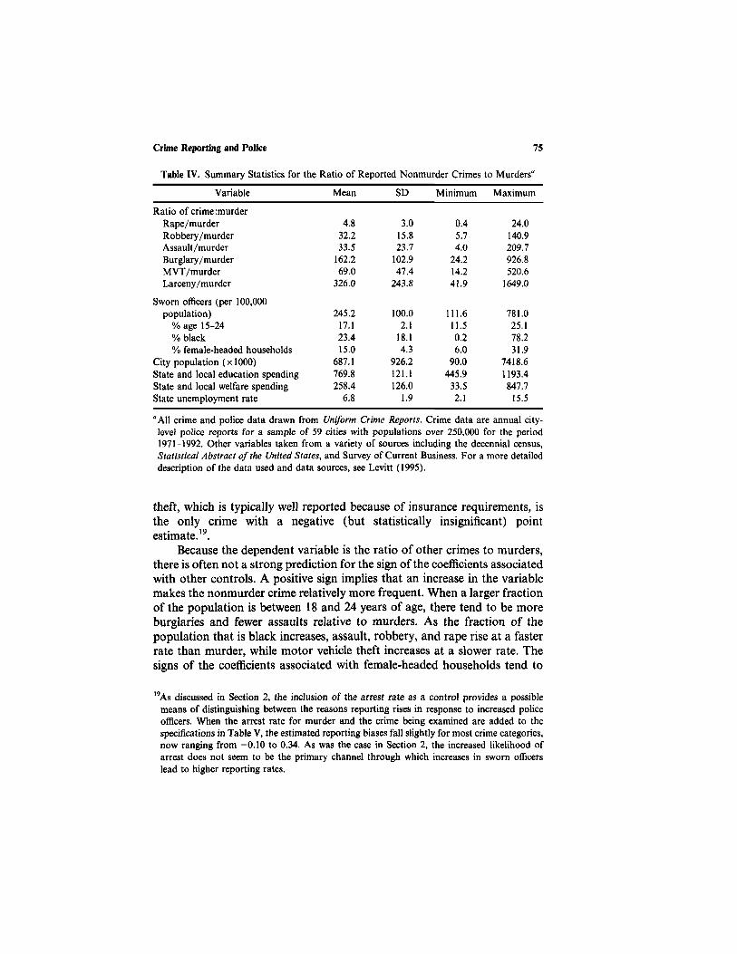
Crime Reporting and Police 75

Table IV. Summary Statistics for the Ratio of Reported Nonmurder Crimes to Murdersa

Variable

Ratio of crime :murderRape/murderRobbery/murderAssault/murderBurglary/murderMVT/murderLarceny /murder

Sworn officers (per 100,000population)

% age 15-24% black% female-headed households

City population (xlOOO)State and local education spendingState and local welfare spendingState unemployment rate

Mean

4.832.233.5

162.269.0

326.0

245.217.123.415.0

687.1769.8258.4

6.8

SD

3.015.823.7

102.947.4

243.8

100.02.1

18.14.3

926.2121.1126.0

1.9

Minimum

0.45.74.0

24.214.241.9

111.611.50.26.0

90.0445.9

33.52.1

Maximum

24.0140.9209.7926.8520.6

1649.0

781.025.178.231.9

7418.61 193.4847.7

15.5

aAll crime and police data drawn from Uniform Crime Reports. Crime data are annual city-level police reports for a sample of 59 cities with populations over 250,000 for the period1971-1992. Other variables taken from a variety of sources including the decennial census,Statistical Abstract of the United States, and Survey of Current Business. For a more detaileddescription of the data used and data sources, see Levitt (1995).

theft, which is typically well reported because of insurance requirements, isthe only crime with a negative (but statistically insignificant) pointestimate.19.

Because the dependent variable is the ratio of other crimes to murders,there is often not a strong prediction for the sign of the coefficients associatedwith other controls. A positive sign implies that an increase in the variablemakes the nonmurder crime relatively more frequent. When a larger fractionof the population is between 18 and 24 years of age, there tend to be moreburglaries and fewer assaults relative to murders. As the fraction of thepopulation that is black increases, assault, robbery, and rape rise at a fasterrate than murder, while motor vehicle theft increases at a slower rate. Thesigns of the coefficients associated with female-headed households tend to

"As discussed in Section 2, the inclusion of the arrest rate as a control provides a possiblemeans of distinguishing between the reasons reporting rises in response to increased policeofficers. When the arrest rate for murder and the crime being examined are added to thespecifications in Table V, the estimated reporting biases fall slightly for most crime categories,now ranging from —0.10 to 0.34. As was the case in Section 2, the increased likelihood ofarrest does not seem to be the primary channel through which increases in sworn officerslead to higher reporting rates.

76 Levitt

Table V. Regression Analysis of Ratios of Reported Nonmurders to Murders"

ln(Sworn Officers)

%age 15-24

% black

% female-headedhouseholds

ln(CityPopulation)

ln(EducationSpending)

ln(WelfareSpending)

State unemploy-ment rate

NAdjusted R2

2SLS coefficient onln(SwornOfficers)

Rape/murder

(1)

0.44(0.14)

-1.81(1.15)0.037

(0.005)

-0.028(0.011)

-0.24(0.19)

-0.33(0.20)

0.01(0.07)

2.62(0.66)

13230.717

l

0.47(0.53)

Robbery/murder

(2)

0.10(0.08)

-5.77(1.01)0.006

(0.004)

-0.022(0.009)

0.08(0.15)

-0.05(0.13)

-0.07(0.04)

3.77(0.48)

13300.727

0.29(0.40)

Assault/murder

(3)

0.30(0.13)

-16.70(1.11)0.021

(0.005)

-0.034(0.011)

-0.50(0.17)

-0.17(0.15)

0.08(0.06)

1.08(0.65)

13300.713

0.34(0.57)

Burglary/murder

(4)

0.40(0.16)1.42

(1.04)-0.016(0.005)

0.014(0.011)

-0.97(0.19)

-0.41(0.20)

-0.12(0.04)

4.63(0.64)

13300.819

0.14(0.44)

Motorvehicle/murder

(5)

-0.01(0.09)

-8.29(0.81)

-0.024(0.004)

0.059(0.009)

-0.11(0.13)

0.59(0.11)

-0.01(0.04)

-0.27(0.51)1330

0.750

0.05(0.46)

Larceny/murder

(6)

0.11(0.14)

-5.56(0.99)0.014

(0.005)

-0.043(0.011)

-0.54(0.17)

-0.15(0.15)

-0.06(0.04)

3.53(0.58)

13300.858

0.17(0.45)

"Dependent variables are ln(Reported Nonmurder Crimes/Reported Murders). Data used area pooled time series of city-level crime reports from Uniform Crime Reports for a sample of59 cities with populations greater than 250,000 over the time periods 1971-1992. City-fixedeffects included in all regressions. Under the assumption that additional police are equallyeffective in reducing murders and other crimes, the coefficient on ln(Sworn Officers) is anestimate of reporting bias for the crime in question. The estimation technique used is weightedleast-squares, with observation rates proportional to city population. Standard errors (inparentheses) have been corrected using White heteroskedasticity-consistent standard errors.The 2SLS coefficient reported in the bottom row is the coefficient on ln(Sworn Officers)instrumenting for the police variables with mayoral and gubernatorial election years by city.

Crime Reporting and Police 77

be reversed from those on percentage black. Given the strong positive corre-lation between those two variables (r=0.86), strong inferences should notbe drawn from those coefficients individually. Increases in population arecorrelated with a greater increase in murders than property crimes. Increasesin spending on education are associated with higher levels of other crimesrelative to murder, while the effects of public welfare spending are mixed.With the exception of motor vehicle theft, other crimes respond more dram-atically to unemployment than do murders.

One concern in interpreting the foregoing analysis is the potentialendogeneity of sworn officers, although the case for endogeneity is not asstraightforward as usual. In the typical regression of police on crime, endog-eneity arises because politicians respond to rising crime by increasing spend-ing on police resources. In the regressions presented in Table V, that aloneis not sufficient to bias the coefficients. Rather, it must be the case that anincrease in murders leads to a different political response than a proportion-ate increase in other, nonmurder crimes. It is possible that politicians aremore responsive to changes in murders than changes in other crimes, whichwould lead to a downward bias in the estimation of the reporting biascoefficient.

In an attempt to counteract that endogeneity, the years of the mayoraland gubernatorial election cycle are used as instruments. To serve as validinstruments, election timing must be correlated with changes in the size ofthe police force but, otherwise, uncorrelated with the ratio of nonmurdersto murder since other covariates are included. Levitt (1997) demonstratesthat increases in big-city police forces are disproportionately concentratedin election years. It is difficult, however, to argue that the election cycle iscorrelated with the ratio of nonmurders to murders, except through changesin the police force.20

The specifications in Table V were therefore reestimated using two-stageleast-squares. The number of sworn officers and arrest rates were treated asendogenous, using the years of the mayoral and gubernatorial election cycleas instruments. The other variables were treated as exogenous. To economizeon space, only the coefficients on sworn officers are presented in the bottomrow in Table V. The other parameter estimates are consistent with the OLSresults, although less precisely estimated. Full results are available from theauthor on request.

The standard errors on the 2SLS parameter estimates are three to fourtimes higher than with OLS due to the instrumenting. Consequently, it isdifficult to draw strong conclusions about individual parameter estimates.

20For complete documentation of the relationship between election cycles and police staffing,as well as details of the estimation of the first-stage equation, see Levitt (1997).

78 Levitt

The overall pattern of coefficients, however, suggests that the results are notvery sensitive to the presence of endogeneity. Four of the six 2SLS estimatesare higher than the corresponding OLS estimates, while two are lower. Themean reporting bias across all crime categories is 0.178 for OLS and 0.215for 2SLS.

5. IMPLICATIONS AND CONCLUSIONS

This paper investigates three data sets in an attempt to measure report-ing/recording bias. While each of the techniques has prominent short-comings, it is reassuring that the three sets of estimates are roughly similarin magnitude. The likelihood that a crime will be officially reported appearsto be an increasing function of the number of sworn officers per capita,although the results are by no means definitive. Of the 30 separate pointestimates of reporting bias presented in this paper, 28 are positive, but only9 are statistically significant at the 0.05 level. The median reporting elasticityobtained in this papers is approximately 0.12; the mean reporting elasticityis 0.16. Assuming a reporting elasticity of 0.12 for all nonmurder crimes,adding one police officer in the typical large city would result in the addi-tional reporting of roughly five Index I crimes that would not previouslyhave been reported. Based on the estimated cost of crime to victims of Cohen(1988), these five crimes represent a social cost of approximately $20,000.Thus, a naive cost-benefit analysis of the value of an additional police officerthat did not take reporting bias into consideration would substantiallyunderestimate the benefits of increasing the police force.

The largest estimates in this paper are obtained in Section V, where thecoefficients capture not only victim reporting behavior and police recordingpractices. This suggests that changes in the diligence of police recordingvictim crime complaints may be an important part of the story. This conjec-ture is consistent with the observation that propensity of victims to reportcrimes to the police has changed little in the NCVS since 1973, but the gapbetween victims' claims of crimes reported to police and the number ofcrimes officially recorded has steadily decreased.21 Better distinguishingbetween crime reporting and recording is a subject that warrants futureattention.

Although the focus of this paper is reporting bias resulting from changesin the size of police forces, parallel arguments can be made for changes inpolicing strategies. Given that the measured impact of changes in policing

2II would like to thank Patrick Langan not only for bringing this fact to my attention, butalso for raising my awareness of the important distinction between reporting and recordingmore generally.

Crime Reporting and Police 79

strategies are often small, ignoring the possibility of reporting bias may leadto overly pessimistic assessments of the value of policy interventions. It iswidely recognized, for instance, that the adoption of "community policing"practices may lead to higher reporting rates, obscuring any benefits associ-ated with the approach. The results of this paper suggest that such considera-tions need to be taken seriously.

ACKNOWLEDGMENTS

I would like to thank Austan Goolsbee, Jonathan Gruber, Lucia Nixon,James Poterba, three anonymous referees, the editors, John Laub andMichael Maltz, and, especially, Patrick Langan for helpful comments andcritiques, the ICPSR for help in obtaining the data, and the National ScienceFoundation for financial support. All remaining errors are my own.

REFERENCES

Biderman, A., and Lynch, J. (1991). Understanding Crime Incidence Statistics: Why the UCRDiverges from the NCS, Springer-Verlag, New York.

Blumstein, A., Nagin, D., and Cohen, J. (1978). Deterrence and Incapacitation: Estimating theEffects of Criminal Sanctions on Crime Rates, National Academy of Sciences, WashingtonDC.

Bottomley, K. and Coleman, C. (1981). Understanding Crime Rates, Gower, Westmead,England.

Cameron, S. (1988). The economics of crime deterrence: A survey of theory and evidence.Kyklos 41:301-323.

Carr-Hill, R. A., and Stern, N. (1979). Crime, The Police and Criminal Statistics, Wiley, NewYork.

Cohen, M. (1988). Pain, suffering, and jury awards: A study of the cost of crime to victims.Law Soc. Rev. 22: 537-555.

Conaway, M. R., and Lohr, S. L. (1994). A longitudinal analysis of factors associated withreporting violent crimes to the police. J, Quant. Criminol. 10: 23-29.

Craig, S. (1987). The deterrent impact of police: An examination of a locally provided publicservice. J. Urban Econ. 21: 298-311.

Devine, J., Sheley, J., and Smith, M. W. (1988). Macroeconomic and social-control policyinfluences on crime rate changes, 1948-1985. Am. Social. Rev. 53: 407-420.

Dilulio, J. (1996). Help wanted: Economics, crime, and public policy. J. Econ. Perspect.10: 3-24.

Donohue, J., and Siegelman, P. (1994). Is the United States at the optimal rate of crime.Mimeo, American Bar Foundation.

Eck, J., and Spelman, W. (1987). Problem Solving: Problem-Oriented Policing in Newport News,Police Executive Research Forum, Washington, DC.

Federal Bureau of Investigation (multiple editions). Uniform Crime Reports, Federal Bureauof Investigation, Washington, DC.

80 Levitt

Glaeser, E., Sacerdote, B., and Scheinkman, J. (1996). Crime and social interactions. Q. J.Econ. III: 507-548.

Gove, W., Hughes, M., and Geerken, M. (1985). Are Uniform Crime Reports a valid indicatorof the Index crimes? An affirmative answer with only minor qualifications. Criminology23:451-501.

Greenwood, M. J., and Wadycki, W. J. (1973). Crime rates and public expenditures for policeprotection: Their interaction. Rev. Soc. Econ. 31: 138-151.

Jensen, G. F., and Karpos, M. A. (1993). Managing rape: Exploratory research on the behaviorof rape statistics. Criminology 31: 363-385.

Kitsuse, J. I., and Cicourel, A. V. (1963). A note on the uses of official statistics. Soc. Problems1:131-139.

Land, K., McCall, P., and Cohen, L. (1990). Structural covariates of homicide rates: Are thereany invariances across time and space. Am. J. Sociol. 95: 922-967.

Levitt, S. D. (1997). Using electoral cycles in police hiring to estimate the effect of police oncrime. Am. Econ. Rev. (in press).

Marvell, T., and Moody, C. (1996). Police levels, crime rates, and specification problems.Criminology 34: 609-646.

Myers, S. (1980). Why are crimes underreported? What is the crime rate? Does it really matter?Soc. Sci. Q. 61: 23-43.

Myers, S. (1982). Crime in urban areas: New evidence and results. J. Urban Econ.11:148-158.

O'Brien, R. (1985). Crime and Victimization Data, Sage, Beverly Hills, CA.O'Brien, R. (1996). Police productivity and crime rates: 1973-1992. Criminology 34: 183-207.Pelinsky, H., and Jesilow, P. (1982). Myths that Cause Crime, Seven Locks Press, Washington,

DC.Rabindra, S., and Pease, K. (1992). Crime, race, and reporting to the police. Howard J. Crim.

Just. 31:192-199.Sampson, R. (1986). Crime in cities: The effects of formal and informal social control. Crime

Just. Rev. Res. 8:271-311.Sampson, R., and Cohen, J. (1988). Deterrent effects of police on crime: A replication and

theoretical extension. Law Soc. Rev. 22: 163-189.Sellin, J., and Wolfgang, M. (1964). The Measurement of Delinquency, Wiley, New York.Sherman, L. (1992). Police and crime control. In Tonry, M., and Morris, N. (eds.), Modern

Policing, University of Chicago Press, Chicago.Singer, S. (1988). The fear of reprisal and the failure of victims to report a personal crime. J.

Quant. Criminol. 4: 289-302.Skogan, W. (1976). Citizen reporting of crime: Some national panel data. Criminology

13:535-549.Skogan, W. (1984). Reporting crime to the police: The status of world research. J. Res. Crime

Delinq. 21:113-137.Sparrow, M. K., Moore, M. H., and Kennedy, D. (1990). Beyond 911: A New Era of Policing,

Basic Books, New York.Swimmer, G. (1974). Measurement of the effectiveness of urban law enforcement: A simulta-

neous approach. South. Econ. J. 40: 618-630.Thaler, R. (1977). An econometric analysis of property crime. J. Public Econ. 8: 37-51.Thaler, R. (1978). A note on the value of crime control: Evidence from the property market.

J. Urban Econ. 5:137-145.United States Department of Justice (1975a). Criminal Victimization Surveys in American Cities,

Government Printing Office, Washington, DC.United States Department of Justice (1975b). Criminal Victimization Surveys in the Nation's

Five Largest Cities, Government Printing Office, Washington, DC.

Crime Reporting and Police 81

United States Department of Justice (1976). Criminal Victimization Surveys in Eight AmericanCities, Government Printing Office, Washington, DC.

United States Department of Justice (1983). Report to the Nation on Crime and Justice, Govern-ment Printing Office, Washington, DC.

Wilson, J. Q., and Boland, B. (1978). The effect of police on crime. Law Soc. Rev. 12: 367-390.

Zedlewski, E. (1983). Deterrence findings and data sources: A comparison of the UniformCrime Reports and the National Crime Survey. J. Res. Crime Delinq. 20: 262-276.