The Price of Future Liquidity:Time-Varying Liquidity in the U.S. Treasury Market

David Goldreich, Bernd Hanke and Purnendu Nathy

First Draft: September 12, 2001

This Draft: June 4, 2002

JEL classi…cation: G12, G14

Keywords: Liquidity, Asset Pricing.

y All three authors are from London Business School, Institute of Finance and Accounting,

Regent’s Park, London NW1 4SA, United Kingdom, Tel.: +44-20-7262-5050, Fax: +44-20-7724-

7875. The authors’ e-mail addresses are as follows: DGoldreich@london.edu, BHanke@london.edu,

and PNath@london.edu. We are grateful to Andrea Buraschi, Elroy Dimson, Tim Johnson, Stephen

Schaefer, Lakshmanan Shivakumar and Ilya Strebulaev for useful comments and discussions and to

seminar participants at Hebrew University, Norwegian School of Management (BI), London Business

School and Tel Aviv University. All errors and omissions are our responsibility.

The Price of Future Liquidity:Time-Varying Liquidity in the U.S. Treasury Market

ABSTRACT. This paper examines the price di¤erences between very liquid on-the-run U.S.

Treasury securities and less liquid o¤-the-run securities over the entire on/o¤ cycle. By comparing

pairs of securities as their relative liquidity varies over time we can disregard any cross-sectional

di¤erences between the securities. Since the liquidity varies predictably over time we are able to

di¤erentiate between current liquidity and expected future liquidity. We show that the more liquid

security is priced higher on average, but that this di¤erence depends on the amount of expected

future liquidity over its remaining lifetime rather than its current liquidity. We measure future

liquidity using both quotes and trades. The measures include bid-ask spread, depth and trading

activity. Examining a variety of liquidity measures enables us to evaluate their relative importance

and identify the liquidity proxies that most a¤ect prices. Although all of the measures are highly

correlated with one another, we …nd that quotes are more important when estimating the e¤ect of

the bid-ask spread and depth on the liquidity premium, while the number of trades and trading

volume is a more important measure of market activity than the number of quotes.

JEL classi…cation: G12, G14

Keywords: Liquidity, Asset Pricing.

1 Introduction and Motivation

Liquidity, the ability to quickly and cheaply trade an asset at a fair price, is thought

to be an important element that a¤ects the value of securities. Ever since Amihud

and Mendelson’s (1986) seminal work, there have been a number of studies showing

that an asset’s liquidity is valued in the market place. These studies1 often compare

similar securities that di¤er in liquidity and show that the more liquid security has a

higher price or lower return.

However, it is often di¢cult to isolate the price premium for liquidity from other

e¤ects when comparing securities. Securities that di¤er in liquidity usually have

other di¤erences that could confound e¤orts to isolate the price e¤ect of liquidity.

For example, the less liquid security might have additional market risk or credit risk.

Less liquid securities might also be subject to more asymmetric information or they

might be subject to di¤ering tax treatments.2 Therefore, cross-sectional studies are

not able to easily distinguish liquidity e¤ects from other security speci…c di¤erences.

While theory would suggest that expected future liquidity should a¤ect prices,

the empirical literature has almost exclusively focused on current liquidity.3 The

empirical literature has, to date, implicitly assumed that a security’s current liquidity

will persist over time. Though this may be a valid assumption in many cases, little

is known empirically about how expected future liquidity a¤ects prices.

Moreover, the notion of liquidity itself is hard to pin down. Some use the term to

describe the narrowness of the bid-ask spread, but it could also refer to market depth,

volume, or other measures of activity in the market. If traders require the ability to1For example, Amihud and Mendelson (1991), Silber (1991), Brenner, Eldor & Hauser (2001),

Dimson & Hanke (2001), Pastor and Stambaugh (2001) and others.2For example, Amihud and Mendelson (1991) argue that the price di¤erence between Treasury

bills and close-to-maturity Treasury notes can be attributed to di¤erences in liquidity. However,

Kamara (1994) and Strebulaev (2001) show that there are other di¤erences, including taxes, that

a¤ect the price di¤erence.3One exception is Amihud’s (2001) analysis of stock returns.

1

transact small quantities immediately, then the quoted bid-ask spread can be used

to measure the price of immediate execution. However, if traders are interested in

transacting large quantities quickly, then measures of depth are more important.

Market participants may be concerned about the amount of time it takes to arrange

a trade. In this case, the number of daily trades, daily volume or similar measures of

market activity may be more relevant.

While all of these notions of liquidity are valid, ultimately, our interest is in which

among them most a¤ect securities’ prices.

In this paper we address these questions by comparing securities whose relative

liquidity varies predictably over time. This allows us to distinguish between current

liquidity and expected future liquidity. By measuring expected future liquidity using

di¤erent measures, we determine the extent to which each of these aspects of liquidity

a¤ects prices. And by following the same securities over time, we may disregard any

cross-sectional di¤erences between securities.

Our purpose is to examine the e¤ects of time-varying liquidity on securities’ prices

with a stress on distinguishing among di¤erent measures of liquidity. First, we show

theoretically that the price of a security is a¤ected by its expected liquidity over its

entire life. Then, we study this empirically, by comparing on-the-run and o¤-the-run

two-year U.S. Treasury notes over the issue cycle. U.S. Treasury securities are ideal

for a study of this type since they go through predictable patterns of liquidity and

illiquidity.

Two-year notes are auctioned monthly, so that at any time there are 24 issues

outstanding. The most recently issued note is referred to as “on-the-run” and attracts

most of the liquidity. Older notes are “o¤-the-run” and are much less liquid. In this

study, we compare the prices of the “on-the-run” note with the most recent “o¤-the-

run” note.

At the beginning of an issue cycle, the on-the-run note is very liquid. The buyer

of such a note can easily sell it during this early period to another investor who will

2

pay a premium for the remaining liquidity. In contrast, towards the end of the cycle,

although the market may still be very liquid, a buyer might expect to eventually sell

the security when it is o¤-the-run and there is no longer a liquidity premium. So

a buyer late in the cycle should pay less of a premium since he will bene…t from a

shorter time of liquidity. Thus, even if liquidity remains at a consistently high level

throughout the on-the-run period, the liquidity premium in the price should decline

over the period.

At each date, we measure the remaining expected liquidity over the life of the

note using various liquidity measures. We document the patterns in prices and liq-

uidity that occur over the issue cycle. Under all the measures, liquidity remains high

throughout the month-long on-the-run period. Around the time the next note is is-

sued, liquidity declines over a number of days until it reaches a new level. The note

remains somewhat illiquid for the rest of its life. We show that the liquidity premium,

the price di¤erence between the on-the-run and the o¤-the-run notes, declines over

the on-the-run cycle and is close to zero at the end of the month.

The measure of concern is the total, (or equivalently, the average) liquidity re-

maining over the asset’s life. At the beginning of the issue cycle, there is a relatively

large amount of expected liquidity remaining. By the end of the cycle, there is little

future liquidity expected. We …nd that the liquidity premium in the price is closely

related to the expected amount of remaining liquidity.

This shows that expected liquidity, rather than just the current level of liquidity,

is priced in the Treasury market. When the di¤erence in liquidity over the lives of

two securities is expected to be large, there is a relatively wide di¤erence in the price

of the two securities. But as the expected di¤erence in liquidity narrows over time,

so does the price di¤erence.

By comparing a pair of Treasury notes and following them through the cycle, we

bypass any problems that might arise if the securities are not otherwise identical. For

example, if the securities we are comparing are taxed di¤erently (for example, due to

3

di¤ering coupons), then there could be a resulting price di¤erence. However, as long

as these di¤erences do not vary systematically over the issue cycle, then the analysis

of the change in the liquidity premium over the cycle is not a¤ected.

As mentioned above, we use various measures of liquidity in this study. These

measures use quotes and trades to capture bid-ask spreads, depth, and the overall

level of market activity. The measures are all correlated with each other and any

one of them explains the changes in price as expected liquidity changes. Our method

allows us to quantify the e¤ect of illiquidity on a security’s value. For example, we

measure the expected (quoted) bid-ask spread over the life of the securities. We …nd

that any change in the remaining average quoted bid-ask spread has more than a

twenty-fold e¤ect on the yield of the note. This compensates for all of the future

trading costs over the life of the security.

We compare the various liquidity measures by testing which have further explana-

tory power beyond the other measures and which are subsumed by other liquidity

measures when explaining the liquidity premium in prices. We …nd that the quoted

spread and the quote size are more important than e¤ective spread and traded size,

respectively. This means that the value that investors place on immediacy – the abil-

ity to trade a quantity of securities quickly – is better measured by the quotes of

market makers who supply liquidity, rather than the actual trade prices and trade

sizes. However, as a measure of market activity, the number of trades and the trade

volume is more related to the liquidity premium than the number of quotes.

Previous Literature

Our study attempts to bridge the gap between two streams of existing literature

on liquidity. The …rst stream of literature is on the impact of liquidity on asset prices

and the second stream is on the behavior of di¤erent aspects of liquidity captured by

di¤erent liquidity proxies.

Studies that belong to the …rst stream of literature include Amihud and Mendel-

4

son (1986), Eleswarapu and Reinganum (1993), Brennan and Subrahmanyam (1996),

Barclay, Kandel and Marx (1997), Eleswarapu (1997), Chordia, Roll and Subrah-

manyam (2000), Datar, Naik and Radcli¤e (1998), Pastor and Stambaugh (2001)

and Amihud (2001). These papers compare market liquidity to ex-post returns on

equities. A number of studies also analyze the impact of liquidity on expected re-

turns. Most of these studies examine the market for bonds and notes, notably Ami-

hud and Mendelson (1991), Warga (1992), Daves and Ehrhardt (1993), Boudoukh

and Whitelaw (1993), Kamara (1994), Krishnamurthy (2001) and Strebulaev (2000).

Silber (1991) looks at restricted (non-traded) equities. Brenner, Eldor and Hauser

(2001) examine currency options that are not traded until maturity and Dimson and

Hanke (2001) examine equity-linked bonds.

Apart from relatively few exceptions (Eleswarapu and Reinganum (1993) and

Barclay, Kandel and Marx (1997)) the general consensus of these studies is that less

liquid securities have higher returns.

Also, the literature on repo markets has shown that U.S. Treasury repos are more

likely to be “special” during the on-the-run period, i.e., there is an increased price

for borrowing the security during this time period. This is consistent with a liquidity

premium in the Treasury market as modeled by Du¢e (1996) and as seen in the

empirical results of Jordan and Jordan (1997) and Buraschi and Menini (2001).

The second stream of literature examines and compares di¤erent aspects of liquid-

ity. Elton and Green (1998) …nd that trading volume as a proxy for liquidity has an

e¤ect on Treasury bond prices. Fleming (1997), Fleming and Remolona (1999) and

Balduzzi, Elton and Green (2000) document intraday patterns of bid-ask spreads and

trading volume but do not link those patterns to prices. Fleming (2001) examines a

set of liquidity measures for the U.S. Treasury market and …nds that price pressure

is closely related to securities’ price changes over very short (…ve-minute) intervals.

Huang, Cai and Song (2001) relate liquidity in the Treasury market to return volatil-

ity. They …nd that the number of trades is more correlated with volatility than is

5

trading volume. Jones, Kaul and Lipson (1994) have similar results for equity mar-

kets. They also …nd that trade size as a determinant of return volatility has little

information beyond that contained in the number of trades.

In general, these studies show that di¤erent aspects of liquidity can be captured

by di¤erent liquidity proxies. Most of the liquidity proxies are highly correlated with

each other but some seem to capture the notion of liquidity better than others.

Studies that belong to this second stream of literature on liquidity su¤er from

two main limitations. First, they only examine the current liquidity rather than

including expected future liquidity which should have the primary e¤ect on prices.

Contemporaneous liquidity measures should only have a signi…cant impact to the

extent that they are proxies for expected future liquidity. In the case of Treasuries, on-

the-run liquidity di¤ers considerably from o¤-the-run liquidity, so contemporaneous

measures are not good proxies for expected liquidity. Second, when these studies

compare two securities, it is di¢cult to isolate return variation due to liquidity changes

from return variation caused by other factors. This study is an attempt to address

these problems and to bridge the gap between the two streams of literature by relating

a clean measure of the liquidity premium to various liquidity proxies.

The rest of this paper is organized as follows: Section 2 is a short theory of the

e¤ect of liquidity on asset prices. Section 3 describes the market and data. Section

4 gives an overview of how liquidity in the Treasury market varies over the on/o¤

cycle. Section 5 describes the details of the methodology. Section 6 contains the

empirical results and Section 7 concludes.

2 Theory of Liquidity and Bond Prices

The theory presented below is based on Amihud and Mendelson (1986).

Illiquidity can be generally thought of as being measured by c, the cost to trade

the security as a proportion of its value. This can represent the bid-ask spread, the

6

opportunity cost of waiting to trade, or any similar cost. Let us assume that this

cost is borne by the seller of the security. Furthermore, suppose that an investor

only trades when hit by an exogenous liquidity shock and let λi be the per-period

probability of investor i being hit with such a liquidity shock.

We will …rst compare a fully liquid zero-coupon bond (i.e., one that has no trading

costs) with a similar bond that has positive trading costs, c. We assume the existence

of a risk-neutral marginal investor m who is indi¤erent between owning the two

securities. This investor has a probability of λm of being hit with a liquidity shock

each period.

The main results shown below are: (1) The value of an illiquid bond is reduced

by the expected trading costs over the entire life of the asset. (2) The expected per-

period proportional trading costs, λmc, can be viewed as a discount rate. Therefore,

the yield of an illiquid bond is equal to the yield of a liquid bond plus λmc. (3) If two

bonds have di¤erent trading costs (which may vary over time), the di¤erence in their

yields is equal to the di¤erence in expected average trading costs to the marginal

investor over the life of the securities.

Let ft be the one period forward rate of interest from time t ¡ 1 to t for the

perfectly liquid bond. Both the liquid and illiquid bond mature at time T at which

time they each pay $1.

At time T ¡ 1, the value of the liquid bond is (by de…nition):

PLT¡1 =

11 + fT

and at any time t,

PLt =

TY

j=t+1

µ1

1 + fj

¶.

At time T ¡1 the owner of the illiquid bond is no longer subject to future liquidity

shocks before maturity and values his bond as

P IT¡1 =

11 + fT

.

7

However, at time T ¡ 2, the owner of the illiquid bond will be concerned about

the probability λm that he will be hit with a liquidity shock at time T ¡ 1 and will

have to pay cP IT¡1. Therefore, the value of the illiquid security at T ¡ 2 is

P IT¡2 = 1

1 + fT¡1

£(1¡ λm)P I

T¡1 + λm (1 ¡ c)P IT¡1

¤

=µ

11 + fT¡1

¶(1¡ λmc)P I

T¡1

= (1 ¡ λmc)PLT¡2.

This value is the expected value of the illiquid bond at T ¡ 1 (less the expected

trading costs) discounted back to T ¡ 2. More simply, the value of the illiquid bond

is equal to the value of the liquid bond discounted by the expected trading costs.

Similarly, at time T ¡ 3, the value of the illiquid bond is

P IT¡3 =

µ1

1 + fT¡2

¶(1¡ λmc)P I

T¡2 = (1¡ λmc)2P LT¡3

and at any time t, the value of the illiquid bond is

P It = (1¡ λmc)T¡t¡1 P L

t

or equivalently,

P It = (1 ¡ λmc)T¡t¡1

TY

j=t+1

µ1

1 + fj

¶.

Until this point, we considered the discrete time case in which there is a point

T ¡ 1 after which there are no longer liquidity shocks. However, if there is always a

probability of a liquidity shock, it becomes simpler to consider the continuous time

case. In continuous time, the value of the illiquid bond is

P It = e

¡TRt(fτ+λmc)dτ

= e¡λmc(T¡t)P Lt (1)

where ft is now the instantaneous forward rate. Equation (1) can be rewritten using

yields, where yLt and yI

t are the yields to maturity for the liquid and illiquid bonds,

respectively. So we have

P It = e¡yI

t (T¡t) = e¡(λmc+yLt )(T¡t). (2)

8

Thus, the relationship between the yields of the two bonds is simply

yIt = λmc+ yL

t . (3)

In words, the yield on an illiquid bond exceeds the yield on a liquid bond simply

by the proportional trading cost times the per-period probability of a liquidity shock

to the marginal investor.

The fact that λmc, the expected per-period trading costs, is added to the bond’s

yield illustrates the similarity between expected transaction costs and interest rates.

Just like an interest rate of r reduces a cash ‡ow’s value at a rate r per period,

similarly, expected transaction costs of λmc per period reduce the value of a cash

‡ow.

The preceding analysis can be generalized to a case in which both assets are

somewhat illiquid (and now denoted as assets A and B) with trading costs cA and

cB, respectively. It is only necessary to assume that there exists a marginal investor

that is indi¤erent between the two assets. In this case the relationship between the

yields of the two assets is

yBt = λm

¡cB ¡ cA¢

+ yAt (4)

Thus the yield spread between the two bonds is proportional to the di¤erence in

trading costs.

We can further generalize to allow for the possibility of transaction costs varying

over time. This is particularly relevant for our study of U.S. Treasury notes, since

the liquidity of the notes does vary systematically over time. We can easily generalize

in this case by a simple adjustment to equation (1), which leads to equation (4) being

rewritten as

yBt = λmEt

³cB ¡ cA

´+ yA

t (5)

where ci is the average trading cost over the life of security i, and Et is the expectations

operator at time t. Now the di¤erence between yields is proportional to the average

di¤erence between the trading costs of the two securities.

9

3 The Market for U.S. Treasury Securities

Description and Data

The United States Treasury sells securities by auction on a regular schedule to …nance

the national debt. The empirical analysis in this study focuses on two-year notes

which are auctioned monthly. Thus, at any time there are 24 issues outstanding.

The issue size averages approximately $16 billion. As explained above, the most

recently issued security of a given maturity is referred to as “on-the-run” and older

securities are referred to as “o¤-the-run”. The “on-the-run” security is considered to

be the benchmark security, and as a result attracts most of the trade and liquidity.

The secondary market is predominantly an over-the-counter market with many

brokers and dealers. During most of the period for which we have data, there were six

major interdealer brokers who allow dealers to trade anonymously with each other.

Quotes are submitted to interdealer brokers who then display the quotes for all

dealers to see. To e¤ect a transaction, a dealer hits a bid or takes an ask that is

displayed. Thus all trade occurs at quotes. However, price improvement e¤ectively

occurs when dealers improve on each other’s quotes while waiting for a counterparty.

In spite of the large number of dealers in the over-the-counter market, the vast

majority of the quoting and trading activity is by less than 40 primary dealers. Pri-

mary dealers are those approved to transact directly with the Federal Reserve in

its market operations. Primary dealers are also expected to participate in Treasury

auctions as well as to make a market for customers.

The data set on the U.S. Treasury market that is used in this study is from

GovPX. GovPX was set up in 1990 by all, except one, interdealer brokers in order

to provide greater transparency in the U.S. Treasury market. The GovPX data set

consists of all trades that are transacted through participating interdealer brokers.

It includes the best bid and ask prices, trade prices, and the size of each trade and

quote. There is no other data set for U.S. Treasury securities that covers a similarly

10

extensive period of intraday quotes and trading activity.4 This study uses data from

January 1994 to December 2000.

Because the GovPX data set is unique in its coverage of the Treasury securities

secondary market, it is important to point out some of its limitations. First, as

mentioned above, the data is from only …ve of the six interdealer brokers. It does

not include trades and quotes routed through Cantor Fitzgerald – the largest of

the interdealer brokers with a market share of about 30%. Cantor Fitzgerald is

particularly strong at the “long end” of the Treasury maturity spectrum. Second,

since the interdealer broker market is anonymous, it is impossible to identify the

counterparties of a transaction or identify the brokers submitting quotations.

4 Overview of Treasury Market Liquidity

Examination of the various measures of liquidity and trading activity over the issue

cycle for the two-year note reveals some interesting patterns. Figures 1 through 4

show how liquidity varies over the …rst 100 trading days of the securities. We measure

time relative to the issue date of each security and average over the cross-section of

securities. The …rst 22 trading days correspond, approximately, to the on-the-run

period.

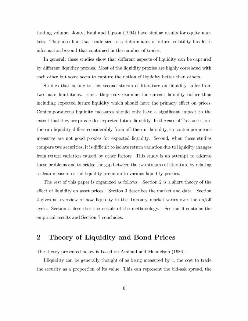
Figure 1 shows the average daily quoted and e¤ective spreads (in yield space)

averaged across the two-year notes in our sample for the …rst 100 days after issue.

The quoted spread is the di¤erence between the best bid and the best ask at any time

and averaged over all quotes in a day. The e¤ective spread is de…ned as twice the

di¤erence between each trade price and the most recent midquote. Since, all trades

occur at the quotes, the e¤ective spread can also be de…ned as the quoted spread

immediately before a trade. The average e¤ective spread is lower than the average4Prior to the availability of GovPX, studies either used quotes collected by the Federal Reserve

Bank of New York from a daily survey of dealers, or small proprietary data sets.

11

quoted spread because trade tends to occur after a narrowing of the spread. During

the …rst 15 trading days the e¤ective spread is in the region of 0.4 basis points, while

the quoted spread is about 0.6 basis points. Over the following week, in the run up

to the issue of the next two-year note, spreads widen and continue to do so as the

life of the security shortens. When the security is o¤-the-run, the e¤ective spread is

mostly above one basis point and the quoted spread averages more than two basis

points. O¤-the-run spreads are considerably more volatile than on-the-run spreads.

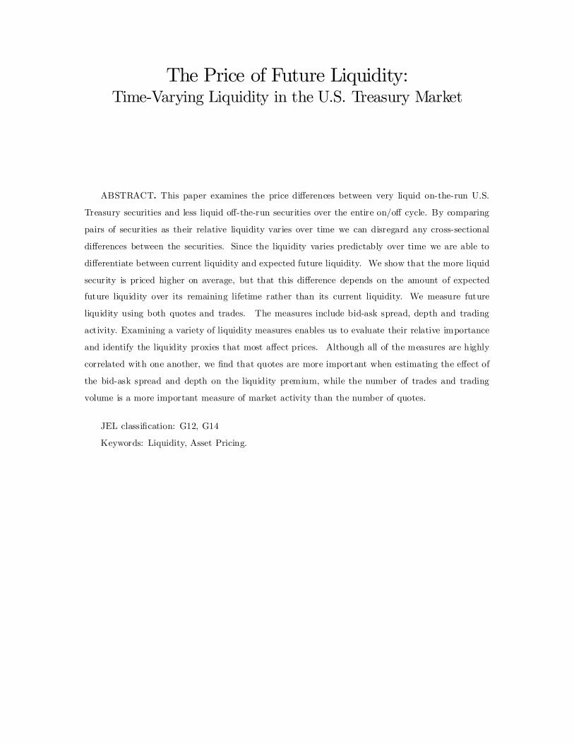
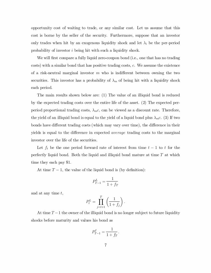
Figure 2 shows the average quote and trade sizes. During the on-the-run period,

quotes average about $20 million and the average transaction size is between $10

million and $15 million. In comparison, during the o¤-the-run period trade size

averages about $7 million while the average quote size falls much further to between

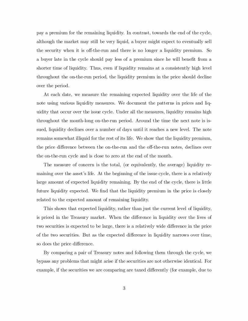
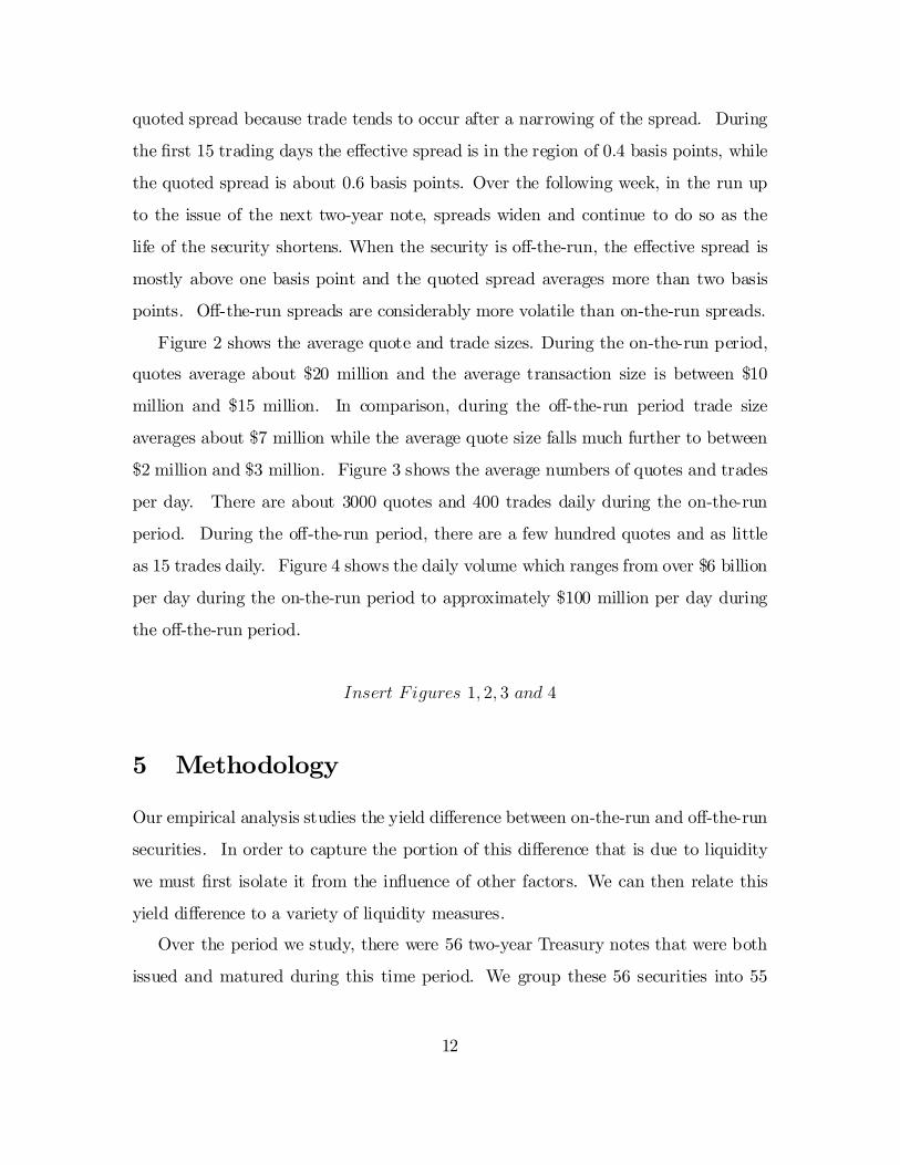
$2 million and $3 million. Figure 3 shows the average numbers of quotes and trades

per day. There are about 3000 quotes and 400 trades daily during the on-the-run

period. During the o¤-the-run period, there are a few hundred quotes and as little

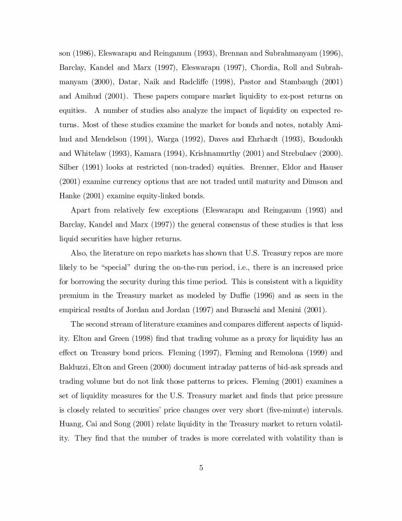
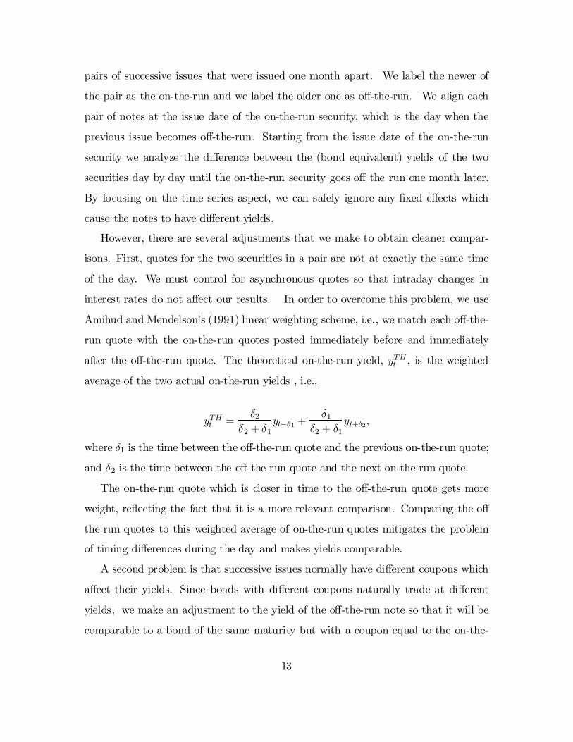
as 15 trades daily. Figure 4 shows the daily volume which ranges from over $6 billion

per day during the on-the-run period to approximately $100 million per day during

the o¤-the-run period.

Insert Figures 1, 2, 3 and 4

5 Methodology

Our empirical analysis studies the yield di¤erence between on-the-run and o¤-the-run

securities. In order to capture the portion of this di¤erence that is due to liquidity

we must …rst isolate it from the in‡uence of other factors. We can then relate this

yield di¤erence to a variety of liquidity measures.

Over the period we study, there were 56 two-year Treasury notes that were both

issued and matured during this time period. We group these 56 securities into 55

12

pairs of successive issues that were issued one month apart. We label the newer of

the pair as the on-the-run and we label the older one as o¤-the-run. We align each

pair of notes at the issue date of the on-the-run security, which is the day when the

previous issue becomes o¤-the-run. Starting from the issue date of the on-the-run

security we analyze the di¤erence between the (bond equivalent) yields of the two

securities day by day until the on-the-run security goes o¤ the run one month later.

By focusing on the time series aspect, we can safely ignore any …xed e¤ects which

cause the notes to have di¤erent yields.

However, there are several adjustments that we make to obtain cleaner compar-

isons. First, quotes for the two securities in a pair are not at exactly the same time

of the day. We must control for asynchronous quotes so that intraday changes in

interest rates do not a¤ect our results. In order to overcome this problem, we use

Amihud and Mendelson’s (1991) linear weighting scheme, i.e., we match each o¤-the-

run quote with the on-the-run quotes posted immediately before and immediately

after the o¤-the-run quote. The theoretical on-the-run yield, yTHt , is the weighted

average of the two actual on-the-run yields , i.e.,

yTHt = δ2

δ2 + δ1yt¡δ1 +

δ1δ2 + δ1

yt+δ2,

where δ1 is the time between the o¤-the-run quote and the previous on-the-run quote;

and δ2 is the time between the o¤-the-run quote and the next on-the-run quote.

The on-the-run quote which is closer in time to the o¤-the-run quote gets more

weight, re‡ecting the fact that it is a more relevant comparison. Comparing the o¤

the run quotes to this weighted average of on-the-run quotes mitigates the problem

of timing di¤erences during the day and makes yields comparable.

A second problem is that successive issues normally have di¤erent coupons which

a¤ect their yields. Since bonds with di¤erent coupons naturally trade at di¤erent

yields, we make an adjustment to the yield of the o¤-the-run note so that it will be

comparable to a bond of the same maturity but with a coupon equal to the on-the-

13

run coupon. This coupon adjustment is simply the di¤erence in yields between two

hypothetical bonds (of the same liquidity) both with same maturity as the o¤-the-run

security but with di¤erent coupons - one with same coupon as the o¤-the-run note and

one with a coupon equal to that of the on-the-run note. We use zero-coupon bond

price data to calculate the yields of these hypothetical securities to obtain the coupon

adjustment. For example, suppose a 24-month on-the-run note has a 6% coupon and

the 23-month o¤-the-run note has a 5.5% coupon. We use the zero-coupon price

data to value a 23-month 5.5% note and a hypothetical 23-month 6% note. For each

of these hypothetical prices we calculate yields. The di¤erence between these two

calculated yields is the coupon adjustment and is added to the actual quoted yield of

the o¤-the-run note. Any small errors in the zero-coupon data appear in the yields

of both hypothetical bonds and only have a negligible e¤ect on the adjustment.

A potentially more serious problem is that the two notes that we compare, al-

though very close in maturity, are not exactly at the same point on the yield curve.

Hence, if the yield curve is not ‡at we would expect them to have di¤erent yields even

in the absence of any liquidity e¤ect. We solve this problem in a manner similar to

the adjustment for the di¤erence in coupons. An adjustment is added to the yield

of the o¤-the-run security for being of a slightly shorter maturity. The adjustment is

equal to the di¤erence between two hypothetical yields: the yield of a security with

a maturity equal to the maturity of the on-the-run and the yield of a security with

a maturity equal to the maturity of the o¤-the-run. The hypothetical yields are ob-

tained from a spline of zero-coupon bond prices. The spline excludes any strip that

has a maturity close to that of the on-the-run security to bypass any liquidity pre-

mium in the zero-coupon data. Again, since the adjustment is a di¤erence between

two yields calculated using the same data, any small data errors have a negligible

e¤ect.

We de…ne the yield e¤ect at each time t for each pair of notes, Y Et, as the yield

of the o¤-the-run security minus the yield of the on-the-run security (adjusted as

14

above).

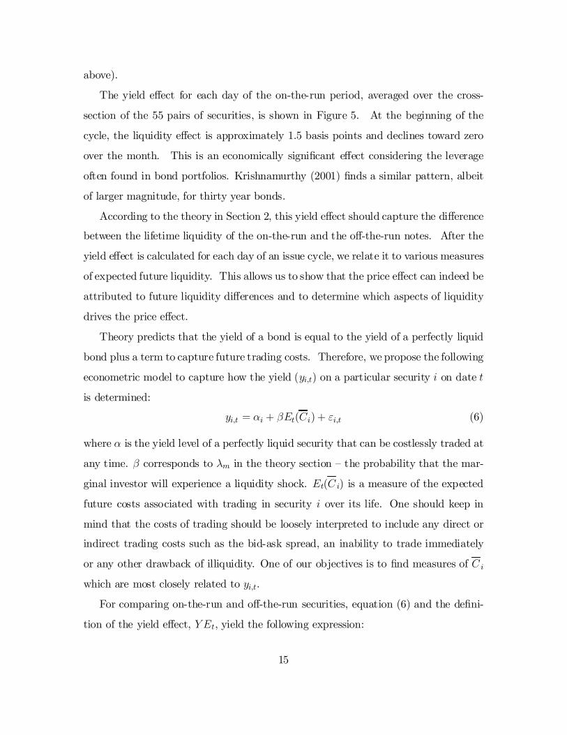
The yield e¤ect for each day of the on-the-run period, averaged over the cross-

section of the 55 pairs of securities, is shown in Figure 5. At the beginning of the

cycle, the liquidity e¤ect is approximately 1.5 basis points and declines toward zero

over the month. This is an economically signi…cant e¤ect considering the leverage

often found in bond portfolios. Krishnamurthy (2001) …nds a similar pattern, albeit

of larger magnitude, for thirty year bonds.

According to the theory in Section 2, this yield e¤ect should capture the di¤erence

between the lifetime liquidity of the on-the-run and the o¤-the-run notes. After the

yield e¤ect is calculated for each day of an issue cycle, we relate it to various measures

of expected future liquidity. This allows us to show that the price e¤ect can indeed be

attributed to future liquidity di¤erences and to determine which aspects of liquidity

drives the price e¤ect.

Theory predicts that the yield of a bond is equal to the yield of a perfectly liquid

bond plus a term to capture future trading costs. Therefore, we propose the following

econometric model to capture how the yield (yi,t) on a particular security i on date t

is determined:

yi,t = αi + βEt(Ci) + εi,t (6)

where α is the yield level of a perfectly liquid security that can be costlessly traded at

any time. β corresponds to λm in the theory section – the probability that the mar-

ginal investor will experience a liquidity shock. Et(C i) is a measure of the expected

future costs associated with trading in security i over its life. One should keep in

mind that the costs of trading should be loosely interpreted to include any direct or

indirect trading costs such as the bid-ask spread, an inability to trade immediately

or any other drawback of illiquidity. One of our objectives is to …nd measures of C i

which are most closely related to yi,t.

For comparing on-the-run and o¤-the-run securities, equation (6) and the de…ni-

tion of the yield e¤ect, Y Et, yield the following expression:

15

Y Et = βEt¡Coff ¡ C on

¢+ ut (7)

which directly corresponds to equation (5) in the theory section.

For each day we calculate the following measures of liquidity:

(a) the average quoted bid-ask spread (in price space),

(b) the average e¤ective bid-ask spread, (i.e. using the bid and ask quotes in price

space immediately before each trade),

(c) the average quote size (in million dollars, where the quote size is measured as

the average of the bid and ask quantities),

(d) the average trade size (in million dollars),

(e) the number of quotes per day,

(f) the number of trades per day, and

(g) the daily volume (in million dollars).5

When we use the spread measures (a) and (b), the trading cost, Ci,t, is calculated

each day as the average of all bid-ask spreads throughout the day. For the other

measures, in order to interpret them as costs, we take (the natural logarithm of) their

reciprocals.

It is an important concept in this paper that the yield e¤ect re‡ects the expectation

of all future trading costs. Because the on/o¤ cycle is so regular and predictable,

we set the average expected future costs, Et(Ci), equal to the average actual cost5Datar, Naik and Radcli¤e (1998) argue that turnover is a more relevant measure than liquid-

ity. This would make little di¤erence in our analysis since all note issues have similar amounts

outstanding.

16

measured from time t until maturity.6 Therefore, for notational simplicity, below we

suppress the expectations operator and we replace it with a time subscript, i.e., Ci,t.

6 Empirical Results

6.1 Basic Regressions

In order to empirically test the relationship between the yield e¤ect and the di¤erence

in expected future liquidity (i.e., equation (7)), we pool the data in a panel that

includes the cross-section of 55 pairs of notes and a month-long time series for each

pair of notes.7 We use a …xed-e¤ects panel-data model to regress the yield e¤ect

(i.e., the adjusted di¤erence between the o¤-the-run and the on-the-run yields) on

the di¤erence in expected future trading costs, Coff,t ¡ Con,t, and a set of dummy

variables (one for each on/o¤ pair). We run individual regressions for each of the

seven cost measures, (as listed at the end of the previous section), using the following

regression model:

Y Et =55X

i=1

αi + β¡Coff,t ¡ Con,t

¢+ εt. (8)

The 55 …xed-e¤ects dummies in each regression are intended to isolate the impact of

expected trading costs from unrelated cross-sectional di¤erences between the securi-

ties.

The fact that we are using an average of trading costs on the right hand side of

the equation introduces signi…cant positive autocorrelation in the regression residuals.

We adjust for autocorrelation in the residuals using a feasible generalized least squares

(FGLS) model for panel data. The regression results for the …rst and second month6Because the data for the last few months before maturity is very noisy, we assume that the costs

during the last six months before maturity are the same as the average over the previous year.7We cannot use time series of longer than one month because the on-the-run security in one pair

of securities becomes the o¤-the-run security for the next pair in the following month.

17

are shown in Table 1.

Insert Table 1

As shown in Panel A of Table 1, for the …rst month, the coe¢cients for each of the

seven expected cost measures are positive and highly signi…cant.8 This shows that

the yield di¤erence between on-the-run and o¤-the-run notes is related to expected

future liquidity regardless of which measure of trading cost we use. The t-statistics for

all variables are similar as well. The fact that all of the cost measures give similarly

signi…cant results should not be surprising since they are highly correlated with each

other.

If the bid-ask spread is interpreted as the cost of trading, then its coe¢cient is an

estimate of the marginal investor’s per-year probability of trading. So, for example,

if the cost of trading is the e¤ective spread, then the yield e¤ect re‡ects a marginal

investor trading more than 60 times per year. In particular, because the individual

time series are run over the …rst month of the new security’s life (although later costs

are included in C i), the coe¢cient should be interpreted primarily as the marginal

investor’s trading propensity over the …rst month.

Because the other cost measures are not literally costs, their coe¢cients do not

lend themselves as easily to interpretation.

The intercepts (not reported) are signi…cantly di¤erent from each other indicating

that there are cross-sectional di¤erences that are not caused by liquidity.

Because of concern for persistence in the construction of the right-hand-side vari-

able, we repeat the analysis with both sides of the regression di¤erenced along the

time-series dimension which removes any …rst-order autocorrelation. Very similar

results are obtained, except that the number of quotes is of only marginal statistical

signi…cance.

The analysis is repeated again using the Fama and MacBeth (1973) procedure8Since we hypothesize a positive relation between the yield e¤ect and costs, the t-statistics should

be interpreted in the context of a one-tailed test.

18

for which we run separate time-series regressions for each pair of securities and av-

erage the coe¢cients across the cross-section. Again, the results are similar and all

coe¢cients are statistically signi…cant.

The regressions in Panel A of Table 1 are run over the …rst month after the issue

of the on-the-run security. In the …rst month, the di¤erence in liquidity between the

on-the-run and the o¤-the-run is striking. In the second month, after an even newer

security is issued, neither security from the original pair is considered on-the-run and

the liquidity di¤erence (and the yield di¤erence) between them is modest.9 Panel

B of Table 1 repeats the above analysis for the second month after the issue of the

on-the-run security.

The basic regressions in the …rst column of Panel B of Table 1 show that while

some of the trading cost measures are signi…cantly related to the yield e¤ect in the

second month, a number of the measures are not. When we di¤erence both sides of

the regression in the time-series dimension, we no longer …nd a relationship between

liquidity and the yield e¤ect. Under the Fama-MacBeth technique, the results are

mixed.

The fact that the model does a poorer job in relating the trading costs to the

yield e¤ect in the second month could be due to the noisier price data in the second

month, and the fact that there is a much smaller yield e¤ect to explain. However,

it is also possible that the marginal investor changes between the …rst month and

the second month. When comparing a new on-the-run with the most recent o¤-

the-run, a marginal investor is one who trades frequently, values liquidity, and is

indi¤erent between the more expensive liquid security and the cheaper less liquid

security. However, in the second month, since there is a newer security that attracts

most of the liquidity, the marginal investor may now be one who trades much less

frequently, values liquidity less, and is choosing between the two securities both of9For consistency, we continue to refer to the newer of the two notes as on-the-run and the older

as o¤-the-run, even though they are now actually o¤-the-run and o¤-o¤-the-run, respectively.

19

which are fairly illiquid. If this is the case, the coe¢cients in the Panel B regressions

should be expected to be smaller than those in Panel A. For the remainder of the

paper, we focus on only the …rst month.

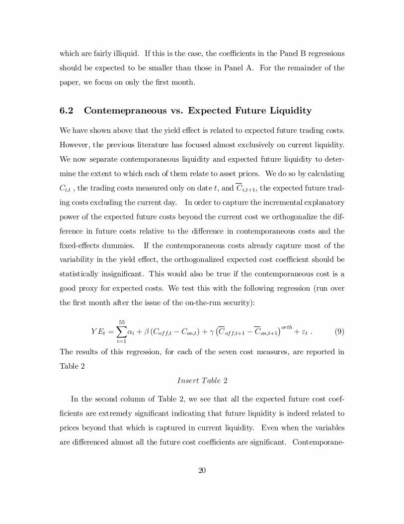
6.2 Contemepraneous vs. Expected Future Liquidity

We have shown above that the yield e¤ect is related to expected future trading costs.

However, the previous literature has focused almost exclusively on current liquidity.

We now separate contemporaneous liquidity and expected future liquidity to deter-

mine the extent to which each of them relate to asset prices. We do so by calculating

Ci,t , the trading costs measured only on date t, and Ci,t+1, the expected future trad-

ing costs excluding the current day. In order to capture the incremental explanatory

power of the expected future costs beyond the current cost we orthogonalize the dif-

ference in future costs relative to the di¤erence in contemporaneous costs and the

…xed-e¤ects dummies. If the contemporaneous costs already capture most of the

variability in the yield e¤ect, the orthogonalized expected cost coe¢cient should be

statistically insigni…cant. This would also be true if the contemporaneous cost is a

good proxy for expected costs. We test this with the following regression (run over

the …rst month after the issue of the on-the-run security):

Y Et =55X

i=1

αi + β (Coff,t ¡ Con,t) + γ¡C off,t+1 ¡ Con,t+1

¢orth + εt . (9)

The results of this regression, for each of the seven cost measures, are reported in

Table 2

Insert Table 2

In the second column of Table 2, we see that all the expected future cost coef-

…cients are extremely signi…cant indicating that future liquidity is indeed related to

prices beyond that which is captured in current liquidity. Even when the variables

are di¤erenced almost all the future cost coe¢cients are signi…cant. Contemporane-

20

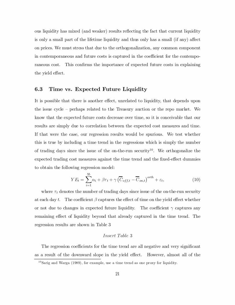
ous liquidity has mixed (and weaker) results re‡ecting the fact that current liquidity

is only a small part of the lifetime liquidity and thus only has a small (if any) a¤ect

on prices. We must stress that due to the orthogonalization, any common component

in contemporaneous and future costs is captured in the coe¢cient for the contempo-

raneous cost. This con…rms the importance of expected future costs in explaining

the yield e¤ect.

6.3 Time vs. Expected Future Liquidity

It is possible that there is another e¤ect, unrelated to liquidity, that depends upon

the issue cycle – perhaps related to the Treasury auction or the repo market. We

know that the expected future costs decrease over time, so it is conceivable that our

results are simply due to correlation between the expected cost measures and time.

If that were the case, our regression results would be spurious. We test whether

this is true by including a time trend in the regressions which is simply the number

of trading days since the issue of the on-the-run security10. We orthogonalize the

expected trading cost measures against the time trend and the …xed-e¤ect dummies

to obtain the following regression model:

Y Et =55X

i=1

αi + βτ t + γ¡Coff,t ¡C on,t

¢orth + εt, (10)

where τt denotes the number of trading days since issue of the on-the-run security

at each day t. The coe¢cient β captures the e¤ect of time on the yield e¤ect whether

or not due to changes in expected future liquidity. The coe¢cient γ captures any

remaining e¤ect of liquidity beyond that already captured in the time trend. The

regression results are shown in Table 3

Insert Table 3

The regression coe¢cients for the time trend are all negative and very signi…cant

as a result of the downward slope in the yield e¤ect. However, almost all of the10Sarig and Warga (1989), for example, use a time trend as one proxy for liquidity.

21

orthogonalized cost measures are also statistically signi…cant. This indicates that

these expected cost measures are not simply proxying for an unrelated time e¤ect.

However, trade size is only weakly signi…cant and the number of quotes is not at all

signi…cant beyond what is already captured in the time trend.

6.4 Comparison of Expected Liquidity Measures

One of the main goals of this paper is to examine the importance of the di¤erent

liquidity measures relative to each other as determinants of the yield e¤ect. If cer-

tain aspects – or certain measures – of illiquidity are more detrimental to investors

than others, then investors will require a higher yield on securities that have these

characteristics.

The main di¢culty in making this comparison is that our trading cost measures

are correlated with each other. In order to examine the relative importance of each,

we run the regression with pairwise combinations of cost measures. For each pair of

cost measures, the di¤erence in expected future costs (between the o¤-the-run and

the on-the-run securities) using the second measure is orthogonalized relative to the

di¤erence in costs under the …rst measure as well as the …xed-e¤ects dummies. The

regression model is

Y Et =55X

i=1

αi + β³C j

off,t ¡ Cjon,t

´+ γ

³Ck

off,t ¡ Ckon,t

´orth+ εt (11)

for j, k = 1, 2, ..., 7 and j 6= k,

where j and k refer to di¤erent cost measures.

Orthogonalizing the two regressors allows us to measure the incremental explana-

tory power of measure k beyond measure j. Given the results in Section 6.1, the

coe¢cient of any measure j will certainly be signi…cantly positive. The question

though, is whether the orthogonalized measure k adds explanatory power or if it is

subsumed by measure j. Since we have seven expected cost measures and we exam-

ine each permutation of pairs we have a total of 42 regressions. The regression results

22

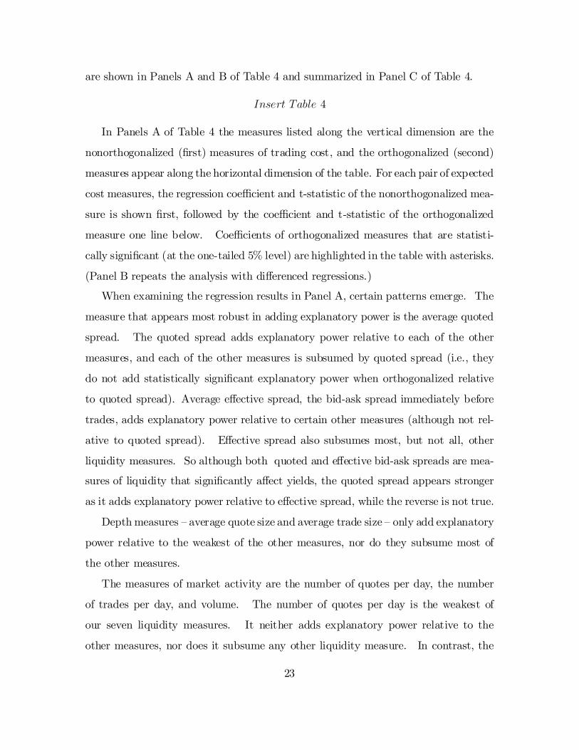
are shown in Panels A and B of Table 4 and summarized in Panel C of Table 4.

Insert Table 4

In Panels A of Table 4 the measures listed along the vertical dimension are the

nonorthogonalized (…rst) measures of trading cost, and the orthogonalized (second)

measures appear along the horizontal dimension of the table. For each pair of expected

cost measures, the regression coe¢cient and t-statistic of the nonorthogonalized mea-

sure is shown …rst, followed by the coe¢cient and t-statistic of the orthogonalized

measure one line below. Coe¢cients of orthogonalized measures that are statisti-

cally signi…cant (at the one-tailed 5% level) are highlighted in the table with asterisks.

(Panel B repeats the analysis with di¤erenced regressions.)

When examining the regression results in Panel A, certain patterns emerge. The

measure that appears most robust in adding explanatory power is the average quoted

spread. The quoted spread adds explanatory power relative to each of the other

measures, and each of the other measures is subsumed by quoted spread (i.e., they

do not add statistically signi…cant explanatory power when orthogonalized relative

to quoted spread). Average e¤ective spread, the bid-ask spread immediately before

trades, adds explanatory power relative to certain other measures (although not rel-

ative to quoted spread). E¤ective spread also subsumes most, but not all, other

liquidity measures. So although both quoted and e¤ective bid-ask spreads are mea-

sures of liquidity that signi…cantly a¤ect yields, the quoted spread appears stronger

as it adds explanatory power relative to e¤ective spread, while the reverse is not true.

Depth measures – average quote size and average trade size – only add explanatory

power relative to the weakest of the other measures, nor do they subsume most of

the other measures.

The measures of market activity are the number of quotes per day, the number

of trades per day, and volume. The number of quotes per day is the weakest of

our seven liquidity measures. It neither adds explanatory power relative to the

other measures, nor does it subsume any other liquidity measure. In contrast, the

23

trade-based measures of market activity – the number of trades and volume – add

explanatory power relative to most of the other measures and subsume most of the

other measures. Although these measures are weakest relative to the quoted spread

and relative to each other.

The results in Table 4, Panel B for di¤erenced regressions are largely similar.

Panel C of Table 4 is a concise summary of the results in Panels A and B. For each

of the liquidity measures, we count the number of times it adds statistically signi…cant

explanatory power (at the one-tailed 5% level) relative to other six measures. We also

count the number of times the measure subsumes the other measures (i.e. that the

other measures do not add statistically signi…cant incremental explanatory power).

From this summary we again see that quoted spread, number of daily trades and

daily volume are most important in explaining the yield e¤ect.

It is curious that when considering the e¤ect of bid-ask spreads on the yields

required by investors, quotes are more important. This may re‡ect the need for

immediacy – the ability to trade a position at any time at the quoted spread without

waiting for the spread to narrow. In contrast, as a measure of market activity, the

number of trades and volume have more of an e¤ect on prices than the number of

quotes. This may capture the time required to …nd a counterparty to complete a

trade at a fair price when immediacy is not needed.

7 Conclusion

This paper examines the e¤ect of liquidity on on-the-run and o¤-the-run U.S. Treasury

notes. Unlike the previous empirical literature, but in line with the theoretical

literature, we focus on expected future liquidity rather than just the current liquidity.

We are able to distinguish between current liquidity and expected future liquidity

because liquidity varies systematically over the on/o¤ cycle in the Treasury market.

At the beginning of the cycle, the on-the-run note is very liquid and can be expected

24

to remain liquid for some time. At the end of the cycle, although the note is still

very liquid it is expected to have little liquidity in the future. We …nd that the price

premium for liquid securities does indeed depend on expected future liquidity.

Our paper also di¤ers from other work in the literature in that we look at the

di¤erences in liquidity and yields of securities over time. Thus any cross-sectional

di¤erence between the securities is merely a …xed e¤ect and so we are able to isolate

the liquidity di¤erences between the securities we are examining.

We measure liquidity using quoted and e¤ective bid-ask spreads; quote and trade

sizes; number of quotes and number trades; and volume. We …nd that each of these

measures signi…cantly explains the yield e¤ect. When orthogonalized relative to each

other, we …nd that the quoted spread and measures of market trading activity, (i.e.,

number of trades and volume) add the most incremental explanatory power relative

to other measures. Depth measures (i.e. average quote and trade size) and especially

the number of daily quotes adds little incremental explanatory power.

25

References

[1] Amihud, Yakov and Haim Mendelson, 1986, Asset pricing and the bid-ask spread,

Journal of Financial Economics 17, 223-249

[2] Amihud, Yakov and Haim Mendelson, 1991, Liquidity, maturity, and the yields

on U.S. Treasury securities, Journal of Finance 46, 1411-1425.

[3] Amihud, Yakov, 2001, Illiquidity and Stock Returns: Cross-Section and Time-

Series e¤ects, Journal of Financial Markets 5, 31-56.

[4] Balduzzi, P., E. J. Elton and T. C. Green, 1997, Economic news and the yield

curve, Working paper, New York University.

[5] Barclay, Michael J., Eugene Kandel and Lesley Marx, 1998, The e¤ects of trans-

action costs on stock prices and trading volume, Journal of Financial Interme-

diation 7, 130-150.

[6] Boudoukh, Jacob and Robert F. Whitelaw, 1993, Liquidity as a choice variable:

a lesson from the Japanese government bond market, Review of Financial Studies

6, 265-292.

[7] Brennan, Michael J. and Avanidhar Subrahmanyam, 1996, Market microstruc-

ture and asset pricing: On the compensation for illiquidity in stock returns,

Journal of Financial Economics 41, 441-464.

[8] Brenner, Menachem, Ra… Eldor and Shmuel Hauser, 2001, The price of options

illiquidity, Journal of Finance, forthcoming.

[9] Buraschi, Andrea and Davide Menini, 2001, Liquidity risk and specialness, Jour-

nal of Financial Economics, forthcoming.

[10] Chordia, Tarun, Richard Roll and A. Subrahmanyam, 2000, Market liquidity

and trading activity, Working paper, UCLA.

26

[11] Datar, Vinay, Naik, Narayan and Robert Radcli¤e, 1998, Liquidity and stock

returns: An alternative test, Journal of Financial Markets 1, 203-219.

[12] Daves, Phillip R. and Michael C. Ehrhardt, 1993, Liquidity, reconstitution, and

the value of U.S. Treasury strips, Journal of Finance 48, 1, 315-329.

[13] Dimson, Elroy and Bernd Hanke, 2001, The expected illiquidity premium: evi-

dence from equity index-linked bonds, Working paper, London Business School.

[14] Du¢e, Darrell, 1996, Special repo rates, Journal of Finance 51, 2, 493-526.

[15] Eleswarapu, Venkat, 1997, Cost of transacting and expected returns in the Nas-

daq market, Journal of Finance 52, 2113-2128.

[16] Eleswarapu, Venkat and Marc Reinganum, 1993, The seasonal behavior of the

liquidity premium in asset pricing, Journal of Financial Economics 34, 281-305.

[17] Elton, E. J. and T. C. Green, 1998, Tax and liquidity e¤ects in pricing govern-

ment bonds, Journal of Finance 53, 1533-1562.

[18] Fama, Eugene F. and James D. MacBeth, 1973, Risk, return and equilibrium:

Empirical tests, Journal of Political Economy 81, 607-636.

[19] Fleming, M. J., 1997, The round-the-clock market for U.S. Treasury securities,

Federal Reserve Bank of New York Economic Policy Review (July), 9-32.

[20] Fleming, M. J., 2001, Measuring Treasury Market Liquidity, Working paper,

Federal Reserve Bank of New York.

[21] Fleming, M. J. and E. M. Remolona, 1999, Price formation and liquidity in the

U.S. Treasury market: The response to public information, Journal of Finance,

1901-1916.

27

[22] Huang, Roger D., Jun Cai, and Xiaozu Wang, 2001, Inventory risk-sharing and

public information-based trading in the Treasury note interdealer broker market,

Working paper, University of Notre Dame and City University of Hong Kong.

[23] Jones, Charles M., Gautam Kaul and Marc Lipson, 1994, Transactions, volume

and volatility, Review of Financial Studies 7, 631-651.

[24] Jordan, Bradford D. and Susan D. Jordan, 1997, Special repo rates: an empirical

analysis, Journal of Finance 52, 5, 2051-2072.

[25] Kamara, Avraham, 1994, Liquidity, taxes, and short-term Treasury yields, Jour-

nal of Financial and Quantitative Analysis 29(3), 403-417.

[26] Krishnamurthy, Arvind, 2001, The bond/old-bond spread, Journal of Financial

Economics, forthcoming.

[27] Pastor, Lubos and Robert Stambaugh, 2001, Liquidity Risk and Expected Stock

Returns, Working paper, University of Chicago.

[28] Sarig, Oded, and Arthur Warga, 1989, Bond price data and bond market liquid-

ity, Journal of Financial and Quantitative Analysis 24, 367-378.

[29] Silber, William , 1991, Discounts on restricted stock: the impact of illiquidity

on stock prices, Financial Analysts Journal 47, 60-64.

[30] Strebulaev, Ilya, 2001, Market imperfections and pricing in the U.S. Treasury

securities market, Working paper, London Business School.

[31] Warga, Arthur, 1992, Bond return, liquidity, and missing data, Journal of Fi-

nancial and Quantitative Analysis 27, 605-617.

28

Figure 1

Quoted Spread and E¤ective Spread

This graph shows the average quoted spread and the average e¤ective spread over the…rst 100 trading days of the two-year US Treasury notes in our sample. Both thequoted and the e¤ective spreads are very low during the on-the-run period (averagingabout 0.6 and 0.4 basis points, respectively) and considerably higher afterwards.

0.0

0.5

1.0

1.5

2.0

2.5

0 20 40 60 80

Trading Days from Issue

Spre

ad in

Bas

is P

oint

s

Quoted Spread Effective Spread

29

Figure 2

Quote Size and Trade Size

This graph shows the average quote size and the average trade size over the …rst 100trading days of the two-year US Treasury notes in our sample. Both quote and tradesize are very high during the on-the-run period (averaging about $20 million and $13million, respectively) and considerably lower afterwards (averaging about $2.5 millionand $6 million, respectively). The quote size declines more rapidly than the tradesize over time. While the average quote size exceeds the average trade size during theon-the-run period, it is lower during the o¤-the-run period.

0.0

5.0

10.0

15.0

20.0

0 20 40 60 80

Trading Days from Issue

Quo

te/T

rade

Siz

e (i

n m

illio

n $)

Quote Size Trade Size

30

Figure 3

Number of Quotes and Number of Trades per Day

This graph shows the average number of quotes and the average number of trades perday over the …rst 100 trading days of the two-year US Treasury notes in our sample.Both the number of quotes and the number of trades are very high during the on-the-run period (averaging about 3,000 and 400 respectively) and considerably lowerafterwards (averaging less than 400 and approximately 15, respectively).

0

500

1000

1500

2000

2500

3000

0 20 40 60 80

Trading Days from Issue

Num

ber

of Q

uote

s/T

rade

s

Number of Quotes Number of Trades

31

Figure 4

Volume per Day

This graph shows the avergae volume per day over the …rst 100 trading days of thetwo-year US Treasury notes in our sample. Volume during the on-the-run period isextremely high compared to the o¤-the-run period (averaging over $6 billion vs. ap-proximately $100 million). There is an abrupt decline in volume at the end of theon-the-run period.

0

1000

2000

3000

4000

5000

6000

7000

0 20 40 60 80

Trading Days from Issue

Vol

ume

(in

mill

ion

$)

Volume

32

Figure 5

Yield E¤ect:

O¤-the-run yield minus on-the-run yield (adjusted)

This graph shows the average di¤erence between the yields of o¤-the-run and on-the-runtwo-year US Treasury notes in our sample. The yield e¤ect is adjusted for di¤erencesin coupon and maturity between each pair of notes. The di¤erence in yields declinesover the month until a newer note is issued.

0.0

0.2

0.4

0.60.8

1.0

1.2

1.4

1.6

1 3 5 7 9 11 13 15 17 19 21

Trading Days from On-the-Run Issue

Bas

is P

oint

s

Yield Effect

33

Table 1Regression of Yield E¤ect on Expected Trading Cost Measures

The …rst column of this table shows the results of autocorrelation-adjusted panel regressionsof the yield e¤ect (Y Et) on the di¤erence between the expected o¤-the-run and the expectedon-the-run cost measures (run separately for each of the seven cost measures). Fifty-…ve…xed-e¤ects dummies are included for each pair of securities in order to isolate cross-sectionaldi¤erences other than liquidity from the impact of the cost measure. The regression equation is

Y Et =55X

i=1

αi + βj

³C j

off,t ¡ Cjon,t

´+ εt for j = 1, 2, ..., 7.

In addition, the same regression is carried out in …rst di¤erences with only one intercept. Wealso run the regressions separately for each pair of securities, average the regression coe¢cients,and calculate the t-statistics using the Fama and MacBeth (1973) procedure. In Panel A, theregressions are run over the …rst month from the issue of the on-the-run security. In Panel B,the regressions are run over the second month.

Panel A: First Month

Cost Measure Panel Regression Panel Regression Fama-MacBeth(Di¤erences)

Quoted Spread 22.12 (10.8) 27.32 (2.6) 10.68 (2.1)E¤ective Spread 66.77 (14.1) 42.46 (2.2) 35.78 (2.2)Quote Size 0.16 (8.9) 0.40 (2.7) 0.09 (2.5)Trade Size 0.43 (11.7) 0.29 (2.1) 0.20 (1.8)# of Quotes 0.18 (7.8) 0.33 (1.6) 0.14 (2.1)# of Trades 0.07 (8.8) 0.22 (3.0) 0.04 (2.4)Volume 0.07 (9.1) 0.19 (3.2) 0.04 (2.3)

Panel B: Second Month

Cost Measure Panel Regression Panel Regression Fama-MacBeth(Di¤erences)

Quoted Spread 0.76 (0.8) -1.09 (-0.6) 6.53 (1.4)E¤ective Spread 35.43 (4.4) 8.59 (0.8) 1.34 (0.1)Quote Size 0.05 (1.8) -0.17 (-1.8) 0.23 (2.8)Trade Size 0.16 (4.3) -0.07 (-1.1) 0.34 (2.7)# of Quotes -0.00 (-0.2) -0.10 (-0.9) 0.57 (1.6)# of Trades -0.05 (-1.5) -0.08 (-1.5) 0.02 (0.1)Volume -0.01 (-0.4) -0.07 (-1.8) 0.06 (0.8)

34

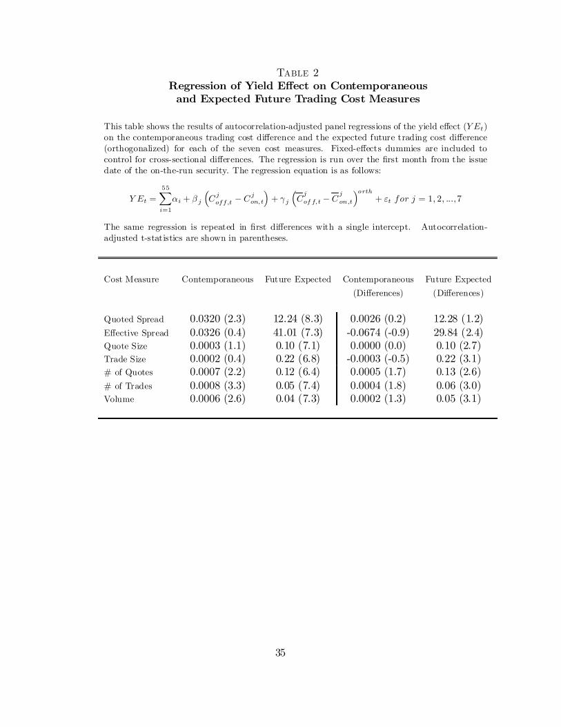
Table 2Regression of Yield E¤ect on Contemporaneousand Expected Future Trading Cost Measures

This table shows the results of autocorrelation-adjusted panel regressions of the yield e¤ect (Y Et)on the contemporaneous trading cost di¤erence and the expected future trading cost di¤erence(orthogonalized) for each of the seven cost measures. Fixed-e¤ects dummies are included tocontrol for cross-sectional di¤erences. The regression is run over the …rst month from the issuedate of the on-the-run security. The regression equation is as follows:

Y Et =55X

i=1

αi + β j

³C j

off,t ¡ C jon,t

´+ γj

³C

jof f,t ¡ C

jon,t

´orth+ εt for j = 1, 2, ...,7

The same regression is repeated in …rst di¤erences with a single intercept. Autocorrelation-adjusted t-statistics are shown in parentheses.

Cost Measure Contemporaneous Future Expected Contemporaneous Future Expected(Di¤erences) (Di¤erences)

Quoted Spread 0.0320 (2.3) 12.24 (8.3) 0.0026 (0.2) 12.28 (1.2)E¤ective Spread 0.0326 (0.4) 41.01 (7.3) -0.0674 (-0.9) 29.84 (2.4)Quote Size 0.0003 (1.1) 0.10 (7.1) 0.0000 (0.0) 0.10 (2.7)Trade Size 0.0002 (0.4) 0.22 (6.8) -0.0003 (-0.5) 0.22 (3.1)# of Quotes 0.0007 (2.2) 0.12 (6.4) 0.0005 (1.7) 0.13 (2.6)# of Trades 0.0008 (3.3) 0.05 (7.4) 0.0004 (1.8) 0.06 (3.0)Volume 0.0006 (2.6) 0.04 (7.3) 0.0002 (1.3) 0.05 (3.1)

35

Table 3Regression of Yield E¤ect on Time Trend

and Expected Trading Cost Measures

This table shows the results of autocorrelation-adjusted panel regressions of theyield e¤ect (Y Et) on a time trend, (i.e., the number of trading days since the issueof the on-the-run note), and the expected trading cost di¤erence (orthogonalized)for each of the seven cost measures. Fixed-e¤ects dummies are included to controlfor cross-sectional di¤erences. The regression is run over the …rst month from theissue of the on-the-run security. Autocorrelation-adjusted t-statistics are shown inparentheses. The regression equation is as follows:

Y Et =55X

i=1

αi + βjTi,t + γj

³C

joff,t ¡ C

jon,t

´orth+ εt for j = 1, 2, ..., 7.

Cost Measure Time Trend Expected Cost

Quoted Spread -0.0002 (-7.3) 22.24 (4.3)E¤ective Spread -0.0003 (-6.5) 40.44 (3.2)Quote Size -0.0002 (-6.8) 0.11 (2.1)Trade Size -0.0003 (-6.7) 0.13 (1.7)Number of Quotes -0.0003 (-6.7) 0.00 (0.0)Number of Trades -0.0003 (-7.7) 0.09 (3.5)Volume -0.0003 (-7.4) 0.06 (3.0)

36

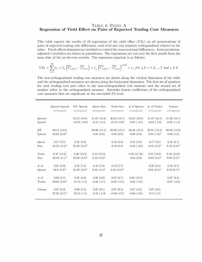
Table 4: Panel ARegression of Yield E¤ect on Pairs of Expected Trading Cost Measures

This table reports the results of 42 regressions of the yield e¤ect (Y Et) on all permutations ofpairs of expected trading cost di¤erences, each with one cost measure orthogonalized relative to theother. Fixed-e¤ects dummies are included to control for cross-sectional di¤erences. Autocorrelation-adjusted t-statistics are shown in parentheses. The regressions are run over the …rst month from theissue date of the on-the-run security. The regression equation is as follows:

Y Et =55X

i=1

αi + βj

³Cj

off,t ¡ Cjon,t

´+ γj

³C k

off,t ¡ Ckon,t

´orth+ εt for j, k = 1, 2, ...,7 and j 6= k.

The non-orthogonalized trading cost measures are shown along the vertical dimension of the tableand the orthogonalized measures are shown along the horizontal dimension. The …rst set of numbersfor each trading cost pair refers to the non-orthogonalized cost measure and the second set ofnumber refers to the orthogonalized measure. Asterisks denote coe¢cients of the orthogonalizedcost measures that are signi…cant at the one-tailed 5% level.

Quoted Spread E¤. Spread Quote Size Trade Size # of Quotes # of Trades Volume(orthogona l) (orthogona l) (orth ogon al) (orth ogon a l) (orthogona l) (orthogona l) (orth ogon al)

Quoted 22.12 (10.8) 21.87 (10.6) 20.62 (10.1) 22.28 (10.8) 21.47 (10.1) 21.30 (10.1)Spread -16.55 (-0.9) -0.14 (-2.1) -0.10 (-0.9) -0.35 (-3.4) -0.04 (-1.0) -0.04 (-1.2)

E¤. 69.14 (14.6) 66.60 (14.1) 65.69 (14.1) 66.46 (14.5) 67.01 (14.2) 66.86 (14.2)Spread 24.62 (3.9)* 0.04 (0.9) 0.08 (0.9) 0.00 (0.0) 0.04 (1.8)* 0.03 (1.6)

Quote 0.17 (9.7) 0.16 (8.6) 0.16 (8.8) 0.15 (8.6) 0.17 (9.5) 0.16 (9.1)Size 34.33 (4.4)* 35.33 (2.2)* 0.10 (0.8) -0.48 (-3.6) 0.19 (3.3)* 0.16 (3.0)*

Trade 0.47 (13.2) 0.46 (12.8) 0.44 (12.3) 0.43 (11.58) 0.45 (12.8) 0.45 (12.8)Size 20.42 (4.1)* 35.98 (2.8)* 0.10 (1.9)* 0.04 (0.6) 0.09 (3.5)* 0.08 (3.5)*

# of 0.21 (8.9) 0.18 (7.4) 0.18 (7.8) 0.18 (7.7) 0.20 (9.4) 0.19 (8.7)Quotes 48.0 (5.2)* 48.20 (2.9)* 0.48 (4.5)* 0.29 (2.4)* 0.38 (6.8)* 0.33 (6.7)*

# of 0.08 (8.7) 0.07 (8.0) 0.08 (9.0) 0.07 (8.7) 0.08 (10.2) 0.07 (8.8)Trades 26.08 (2.9)* 21.74 (1.3) -0.24 (-2.1) -0.02 (-0.2) -0.82 (-5.8) -0.07 (-0.6)

Volume 0.07 (9.2) 0.06 (8.4) 0.07 (9.1) 0.07 (9.2) 0.07 (9.8) 0.07 (9.3)27.56 (3.1)* 23.13 (1.4) -0.24 (-1.9) -0.09 (-0.7) -0.86 (-5.6) 0.15 (1.2)

37

Table 4: Panel BRegression of Yield E¤ect on Pairs of Expected Trading Cost Measures

(Di¤erenced regressions)

This panel repeats the analysis of Panel A in …rst di¤erences and with a single intercept.

Quoted Spread E¤. Spread Quote Size Trade Size # of Quotes # of Trades Volume(orthogona l) (orthogona l) (orth ogon a l) (orthogona l) (orthogona l) (orthogona l) (orthogona l)

Quoted 27.74 (2.7) 48.05 (3.1) 33.51 (3.1) 30.60 (1.9) 47.52 (3.2) 50.74 (3.5)Spread 21.39 (0.9) 0.29 (1.8)* 0.23 (1.6) 0.06 (0.3) 0.16 (1.9)* 0.15 (2.2)*

E¤. 66.54 (2.8) 104.06 (3.0) 59.74 (2.8) 75.58 (2.0) 108.73 (3.3) 114.81 (3.5)Spread 20.95 (1.7)* 0.34 (2.2)* 0.25 (1.8)* 0.21 (1.0) 0.18 (2.4)* 0.17 (2.7)*

Quote 0.46 (3.0) 0.42 (2.8) 0.41 (2.7) 0.43 (2.4) 0.52 (3.2) 0.53 (3.3)Size 19.34 (1.7)* 30.64 (1.5) 0.18 (1.2) 0.06 (0.3) 0.16 (1.8)* 0.15 (2.0)*

Trade 0.56 (3.1) 0.42 (2.7) 0.71 (2.9) 0.53 (2.0) 0.77 (3.2) 0.79 (3.2)Size 24.29 (2.3)* 37.35 (1.9)* 0.34 (2.1)* 0.24 (1.1) 0.19 (2.5)* 0.20 (2.5)*

# of 0.35 (1.7) 0.35 (1.7) 0.54 (2.3) 0.37 (1.7) 0.53 (2.4) 0.54 (2.5)Quotes 25.72 (2.1)* 36.76 (1.8)* 0.38 (2.2)* 0.25 (1.7)* 0.22 (2.6)* 0.21 (2.9)*

# of 0.22 (3.1) 0.22 (3.1) 0.26 (3.2) 0.22 (3.1) 0.21 (2.5) 0.23 (3.2)Trades 15.02 (1.2) 26.82 (1.3) 0.21 (1.1) 0.18 (1.2) -0.04 (-0.2) 0.18 (1.2)

Volume 0.20 (3.4) 0.20 (3.3) 0.22 (3.3) 0.19 (3.1) 0.18 (2.6) 0.20 (3.2)13.96 (1.2) 25.42 (1.3) 0.17 (0.9) 0.00 (0.0) -0.08 (-0.3) 0.02 (0.1)

38

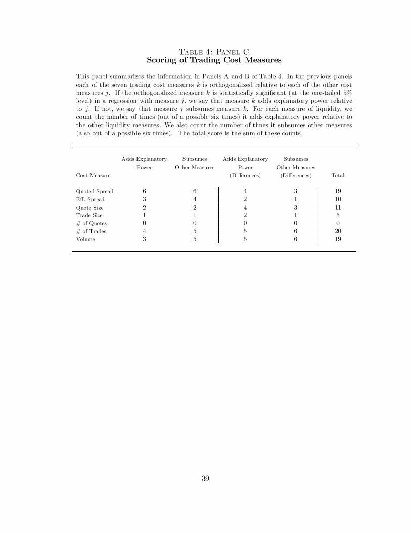
Table 4: Panel CScoring of Trading Cost Measures

This panel summarizes the information in Panels A and B of Table 4. In the previous panelseach of the seven trading cost measures k is orthogonalized relative to each of the other costmeasures j. If the orthogonalized measure k is statistically signi…cant (at the one-tailed 5%level) in a regression with measure j , we say that measure k adds explanatory power relativeto j. If not, we say that measure j subsumes measure k. For each measure of liquidity, wecount the number of times (out of a possible six times) it adds explanatory power relative tothe other liquidity measures. We also count the number of times it subsumes other measures(also out of a possible six times). The total score is the sum of these counts.

Adds Explanatory Subsumes Adds Explanatory SubsumesPower Other Measures Power Other Measures

Cost Measure (Di¤erences) (Di¤erences) Total

Quoted Spread 6 6 4 3 19E¤. Spread 3 4 2 1 10Quote Size 2 2 4 3 11Trade Size 1 1 2 1 5# of Quotes 0 0 0 0 0# of Trades 4 5 5 6 20Volume 3 5 5 6 19

39