The Power of TV: Cable Television and Women’s Status in India

Robert JensenWatson Institute for International Studies, Brown University and NBER

Emily Oster∗

University of Chicago and NBER

July 30, 2007

Abstract

Cable and satellite television have grown rapidly throughout the developing world. Theavailability of cable and satellite television exposes viewers to new information about the outsideworld, which may affect individual attitudes and behaviors. This paper explores the effect of theintroduction of cable television on gender attitudes in rural India. Using a three-yearindividual-level panel dataset, we find that the introduction of cable television is associated withimprovements in women’s status. We find significant increases in reported autonomy, decreases inthe reported acceptability of beating and decreases in reported son preference. We also findincreases in female school enrollment and decreases in fertility (primarily via increased birthspacing). The effects are large, equivalent in some cases to about five years of education in thecross section, and move gender attitudes of individuals in rural areas much closer to those inurban areas. We argue that the results are not driven by pre-existing differential trends. Theseresults have important policy implications, as India and other countries attempt to decrease biasagainst women.

1 Introduction

The growth of television in the developing world over the last two decades has been extraordinary.

Estimates suggest that the number of television sets in Asia has increased more than six-fold, from

100 million to 650 million, since the 1980s (World Press Review, 2003). In China, television exposure

grew from 18 million people in 1977 to 1 billion by 1995 (World Press Review, 2003). In more recent

years, satellite and cable television availability has increased dramatically. Again, in China, the

number of people with satellite access increased from just 270,000 in 1991 to 14 million by 2005.

Further, these numbers are likely to understate the change in the number of people for whom

television is available, since a single television is often watched by many.

Beyond providing entertainment, television vastly increases both the availability of

information about the outside world and exposure to other ways of life, particularly in otherwise∗Matthew Gentzkow, Larry Katz, Steve Levitt, Divya Mathur, Ben Olken, Andrei Shleifer, Jesse Shapiro and partic-

ipants in a seminar at the University of Chicago provided helpful comments.

1

isolated areas. Previous work has demonstrated that the information and exposure provided by

television can change attitudes and behavior. Gentzkow and Shapiro (2005) find effects of television

viewership on attitudes in the Muslim world towards the West, and Della Vigna and Kaplan (2006)

show large effects of the Fox News channel on voting patterns in the United States. In the

developing world, Olken (2006) shows that television decreases participation in social organizations.

India has not been left out of the satellite revolution: a recent survey finds that 112 million

households in India own a television, with 61 percent of those homes having cable or satellite service

(National Readership Studies Council 2006). This figure represents a doubling in cable access in just

five years from a previous survey. The study also find that in some states, the change has been even

more dramatic; in the span of just 10-15 years since it first became available, cable or satellite

penetration has reached an astonishing 60 percent in states such as Tamil Nadu, even though the

average income is below the World Bank poverty line of two dollars per person per day.

Most popular satellite television shows in India portray life in urban settings; further, a wide

range of international programs are now available. The increase in television exposure, therefore, is

likely to dramatically change the available information about the outside world, especially in isolated

rural areas. Indeed, anthropological case studies in India suggest that exposure to television in rural

areas has an effect on behaviors as disparate as latrine building and fan usage (Johnson, 2001).

In this paper we explore the effect of the introduction of cable television in rural areas of

India on a particular set of values and behaviors, namely attitudes towards and discrimination

against women. Although issues of gender equity are important throughout much of the developing

world, they are particularly salient in India. Sen (1992) argued that there were 41 million “missing

women” in India – women and girls who died prematurely due to mistreatment – resulting in a

dramatically male-biased population. The population bias towards men has only gotten worse in the

last two decades, as sex-selective abortion has become more widely used to avoid female births (Jha

et al, 2006). More broadly, girls in India are discriminated against in nutrition, medical care,

vaccination and education (Basu, 1989; Griffiths et al, 2002; Borooah, 2004; Pande, 2003; Mishra et

al, 2004; Oster, 2007). Even within India, gender inequality is significantly worse in rural than urban

areas. Given this, if satellite television increases the exposure of rural areas to urban attitudes and

values, it is plausible that it could change some of these attitudes and behaviors. It is this possibility

that we explore in this paper.

The analysis relies on a three-year panel dataset covering women in five Indian states

between 2001 and 2003. These years represent a time of rapid growth in rural cable access. During

2

the panel, cable television was newly introduced in 21 of the 180 sample villages.1 Our empirical

strategy relies on comparing changes in attitudes and behaviors between survey rounds across

villages based on whether (and when) they added cable television.

Using these data, we find that cable television has large effects on attitudes and, to the

extent we have information, behaviors. After cable is introduced to a village, women are less likely to

report that domestic violence towards women is acceptable. They also report increased autonomy

(for example, the ability to go out without permission and to participate in household

decision-making). Women are less likely to report son preference (the desire to give birth to a boy

rather than a girl). Turning to behaviors, we find increases in school enrollment for girls (but not

boys), and decreases in fertility (which is often linked to female autonomy). These results are

apparent when using regressions with individual fixed effects and when using a matching estimator.

In terms of magnitude, the introduction of cable television dramatically decreases the

differences in attitudes and behaviors between urban and rural areas – between 45 and 70 percent of

the difference disappears within two years of cable introduction in this sample. The effect is also

large relative to, for example, the effect of education on these attitudes and behaviors: introducing

cable television is equivalent to roughly five years of female education in the cross section. These

effects happen very quickly; the average village has cable for only 6-7 months before being surveyed

again, which implies a rapid change in attitudes. However, this is consistent with existing work on

the effects of media exposure, which typically find rapid changes (within a few months, in many

cases) in behaviors like contraceptive use, pregnancy, latrine building and perception of own-village

status (Pace, 1993; Johnson, 2001; Kane et al, 1994; Valente et al, 1998; Rogers et al, 1999).

A central concern with the results is the possibility that trends in other variables (for

example, income or “modernity”) are driving both cable access and attitudes. We argue that this

does not seem to the case. Changes in attitudes between the first two survey waves are not

predictive of cable introduction between the second and third wave. Further, among villages that

add cable during the survey period, initial attitudes are not predictive of which year (2002 or 2003)

they get access.

It is difficult to identify the mechanism behind the effects in this paper precisely. However,

we do find some suggestive evidence that the mechanism alluded to at the start of the paper –1Cable television in these villages is generally introduced by an entrepreneur, who purchases a satellite dish and

subscription, and then charges people (generally within 1km of the dish) to run cables to it. In this sense, people areactually accessing satellite channels. We will use the terms cable and satellite interchangeably to refer to programmingnot available via public broadcast signals. Our interest is with the content of programming available to households,rather than the physical means of delivery of that content.

3

increased exposure to circumstances outside of the village – is operating. In particular, we find that

the effects of cable are largest in areas with initially worse attitudes towards women, i.e., those for

whom cable is providing information most different from their current way of life. Although certainly

not conclusive, this evidence is consistent with a model in which television changes the weight

individuals put on the behaviors of their immediate peer group in forming their attitudes.

The results are potentially quite important for policy. Gender discrimination in India is a

significant issue, and has been a consistent source of concern for policy makers and academics (Sen,

1992; World Bank, 2001; Duflo, 2005; World Bank, 2006). A large literature in economics, sociology

and anthropology has explored the underlying causes of discrimination against women in India,

highlighting the dowry system, low levels of female education, and other socioeconomic factors as

central factors (Rosenzweig and Shultz, 1982; Agnihotri, 2000; Agnihotri et al., 2002; Murthi et al.,

1995; Rahman and Rao, 2004; Qian, 2006). Changing these underlying factors is difficult;

introducing television, or reducing any barriers to its spread, may be less so.

From the policy perspective, however, there are potential concerns about whether the

changes in reported autonomy, beating attitudes, and son preference actually represent changes in

behaviors, or just in reporting. For example, we may be concerned that exposure to television only

changes what the respondent thinks the interviewer wants to hear about the acceptability of beating,

but does not actually change how much beating is occurring. This concern is likely to be less

relevant in the case of fertility or education; the former is directly verifiable based on the presence of

a baby in the household, and the latter is listed as part of a household roster. The fact that we find

effects on these variables provides support for the argument that our results represent real changes in

outcomes. Without directly observing people in their homes, however, it is difficult to conclusively

separate changes in reporting from changes in behavior. However, even if cable only changes what is

reported, it still may represent progress: changing the perceived “correct” attitude seems like a

necessary, if not sufficient, step toward changing outcomes.

The remainder of the paper is organized as follows. Section 2 provides background on

television in India and discusses existing anthropological and ethnographic evidence on the impact of

television on Indian society. Section 3 describes the data and empirical strategy. Section 4 discusses

the results, including the effects on attitudes and behaviors, and robustness checks. Section 5 briefly

explores the possible mechanisms behind the change in attitudes and behaviors, and Section 6

concludes.

4

2 Background on Television in India

State-run black and white television was introduced into India in 1959, but the take off was

extremely slow for the first several decades – by 1977, only around 600,000 sets had been sold. In

1982, however, the state-run broadcaster (Doordarshan) introduced color television, which

dramatically increased interest in, and viewership of, television. Even with color, however, most

programming remained either government-sponsored news or information about economic

development. There were a few entertainment serials, which were watched with intensity.2 In the

early 1990s CNN and STAR TV first introduced the possibility of access to non-government

programming via satellite. There was a large demand for this cable (satellite) television, which was,

and continues to be, filled primarily by small entrepreneurs who buy a dish and a subscription and

charge nearby homes to connect to it. This is especially true in rural villages, such as those in our

sample. As we show in the data later, this means that cable access is more common in villages that

are wealthier and have a higher population density, where more people can afford to pay for service

and where it would therefore be more profitable to start a cable business. However, dramatic declines

in the prices of both the equipment and satellite service subscriptions (due in part to reduced tariffs

and increased competition), coupled with income growth, have allowed cable to spread over time to

more and more villages. In the 5 years from 2001 to 2006, about 30 million households, representing

approximately 150 million individuals, added cable service (National Readership Studies Council

2006). And since television is often watched with family and friends by those without a television or

cable, the growth in actual access or exposure to cable may have been even more dramatic.

The program offerings on cable television are quite different than government programming.

The most popular shows tend to be game shows and soap operas. As an example, among the most

popular shows in both 2000 and 2007 (based on Indian Nielsen ratings) is “Kyunki Saas Bhi Kabhi

Bahu Thi,” (Because a Mother-in-Law was Once a Daughter-in-Law, Also) a show based around the

life of a wealthy industrial family in the large city of Mumbai. As can be seen from the title, the

main themes and plots of the show often revolve around issues of family and gender. Among satellite

channels, STAR TV and Zee TV tend to dominate, although Sony, STAR PLUS and Sun TV are

also represented among the top 20 shows. Viewership of the government channel, although relatively

high among those who do not have cable, is extremely low among those who do (and limited largely

to sporting events).2This background information detailed here is drawn largely from Mankekar, 1999 and

http://www.indiantelevision.com/indianbrodcast/history/historyoftele.htm

5

The introduction of television in general appears to have had large effects on Indian society.

In contrast to the West, television seems to be, in some cases, the primary medium by which people

in rural villages in India get information about the outside world (Scrase, 2002; Mankekar, 1993;

Mankekar, 1998; Johnson, 2001; Fernandes, 2000). For example, Johnson (2001) reports on a man in

his 50’s in a village in India who says that television is “the biggest thing to happen in our village,

ever”. He goes on to say that he learned about the value of electric fans (to deal with the heat) from

television, and subsequently purchased one. The same author quotes another man arguing that

television is where they learned that their leaders were corrupt, and about using the court system to

address grievances.

On issues of gender specifically, television seems to have had a significant impact, since this

is an area where the lives of rural viewers differ greatly from those depicted on most popular shows.

By virtue of the fact that the most popular Indian serials take place in urban settings, women

depicted on these shows are typically much more emancipated than rural women. For example,

many women on popular serials work outside the home, run businesses and control money. In

addition, they are typically more educated and have fewer children than their rural counterparts.

Further, in many cases there is access to Western television, with its accompanying depiction of life

in which women are much more emancipated. Based on anthropological reports, this seems to have

affected attitudes within India. Scrase (2002) reports that several of his respondents thought

television might lead women to question their social position and might help the cause of female

advancement. Another woman reports that, because of television, men and women are able to “open

up a lot more” (Scrase, 2002). Johnson (2001) quotes a number of respondents describing changes in

gender roles as a result of television. One man notes, “Since TV has come to our village, women are

doing less work than before. They only want to watch TV. So we [men] have to do more work. Many

times I help my wife clean the house.”

Although television overall seems to have had large effects, cable television in particular

may be even more significant. This is both because it dramatically increases television viewership

(see Section 3), and because the content is very different (again, since popular serials mostly feature

urban life). Scrase (2002) reports on respondents who note that prior to cable there was almost no

entertainment, and very little current affairs, whereas the offerings on cable were broad.

There is also a broader literature on the effects of television exposure on gender issues in

other countries. Many studies find effects on a variety of outcomes: for example, eating disorders in

Fiji (Becker, 2004), sex role stereotypes in Minnesota (Morgan and Rothschild, 1983) and

6

perceptions of women’s rights in Chicago (Holbert, Shah and Kwak, 2003). Telenovelas in Brazil

have provided a fruitful context for studying the effects of television. For example, based on

ethnographic research, La Pastina (2004) argues that exposure to telenovelas provides women (in

particular) with alternative models of what role they might play in society. Pace (1993) describes the

effect of television introduction in Brazil on a small, isolated, Amazon community, arguing that the

introduction of television changed the framework of social interactions, increased general world

knowledge and changed people’s perceptions about the status of their village in the wider world.

Kottak (1990) reports on similar data from isolated areas in Brazil, and argues that the introduction

of television affects (among other things) views on gender, moving individuals in these areas towards

having more liberal views on the role of women in both the workplace and in relationships.

Interestingly, the studies in Brazil also suggest that the patterns of television viewing

shortly after it is first introduced may be quite different than what is seen later on. The evidence

suggests that in the first years after introduction, interactions with the television are more intense,

with the television drawing more focus (both at an individual level, and community-wide). It is

during this early period that Kottak (1990) and others argue that television is at its most influential.

Most of the villages in our analysis are at this early stage of television exposure, suggesting this may

be an ideal period to look for effects.

The evidence described above, of course, is drawn primarily from interviews and case

studies, and obviously does not reflect a random sample of these populations. Nevertheless, the

overall impression given by the anthropology and sociology literature is that the introduction of

television had widespread effects on society, and that gender issues are a particular focal point. Our

data and setting provide an opportunity to test this hypothesis more rigorously.

3 Data and Empirical Strategy

3.1 Data

This paper relies on data from the Survey of Aging in Rural India (SARI), a panel survey of 2,700

households, each containing a person aged 50 or older, conducted in 2001, 2002 and 2003 in four

states (Bihar, Goa, Haryana,and Tamil Nadu), and the capital, Delhi. The sample was selected in

two stages: in the first stage, 180 clusters were selected at random from district lists (40 clusters in

Bihar, Haryana and Tamil Nadu, 35 in Delhi and 25 in Goa), and in the second stage, 15 households

were chosen within each cluster through random sampling based on registration lists. Other than

7

Delhi, the survey was confined to rural areas. Attrition over the panel was low, with just 108 (4

percent) of the original households dropping out by the third round.

All women in the sample households aged 15 and older were interviewed. Several sections of

this survey were modeled to be compatible with other demographic surveys for India, such as the

National Family and Health Survey (NFHS). The survey collected information on a range of (current

and past) demographic, social and economic variables. In addition, a village-level survey was

conducted in each sample cluster, gathering information on economic and social conditions and

infrastructure.

Most relevant for our analysis, the survey asked women a series of questions intended to

measure various dimensions of women’s status. These questions were patterned after those used in

several countries as part of the Demographic and Health Surveys, as well as in the Surveys on the

Status of Women and Fertility conducted by the University of Pennsylvania Population Studies

Center. The first set of questions deal with women’s autonomy and decision-making authority. In

particular, women were asked whether they needed permission to visit the market (one question) or

to visit friends or relatives (a second question). Responses were coded on a scale of 1 to 3 (do not

need permission; need permission; not permitted at all). Women were also asked whether they are

allowed to keep money set aside to spend as they wish. In addition, women were asked, “Who makes

the following decisions in your household: Obtaining health care for yourself; purchasing major

household items; whether you visit or stay with family members or friends?” The possible responses

were: “1. Respondent; 2. Husband; 3. Respondent jointly with husband; 4. Other household

members; 5. Respondent jointly with other household members.”

Second, women were asked about son preference. In particular, women who reported

wanting to have more children were asked: “Would you like your next child to be a boy, a girl or it

doesn’t matter?”

Finally, given the high prevalence of domestic violence in India, women were asked their

attitudes towards such behavior. Specifically, they were asked: “Please tell me if you think that a

husband is justified in beating his wife in each of the following situations: If he suspects her of being

unfaithful; if her natal family does not give expected money, jewelry or other things; if she shows

disrespect for him; if she leaves the home without telling him; if she neglects the children; if she

doesn’t cook food properly.”

While these measures suffer from obvious limitations, in particular because they are

susceptible to reporting bias, they were designed to capture as best as possible various dimensions of

8

women’s status, and to be consistent with the other major surveys on women’s status. However,

recognizing the limitations, in our analysis we will also make use of measures of behaviors as

indicators for, or proxies of, women’s status, including fertility and girls’ school enrollment. Both

behaviors are linked to women’s status. Female education is generally higher in areas where women

have higher status and, importantly, is itself an input to the health and education of future

generations of women (and men). Lower fertility is often linked to female autonomy (Dyson and

Moore, 1983; Sen, 1999), in part because the value of women’s time increases as the set of activities

they are permitted to do goes up. And while observed changes in fertility may represent direct

changes in attitudes regarding the optimal number or spacing of children independent of changes in

attitudes towards women, reductions in fertility or increased spacing is a useful outcome measure in

itself because it represents gains to women, in the form of reduced health risks and increased

opportunities outside of the home due to reduced child-rearing burdens.

Data on Cable Television

Crucially for this project, the village-level survey included information on cable television. Panel A

of Table 1 provides information on cable availability throughout the survey. In the first round, 65 of

the 180 villages have cable. As stated above, this was a period of rapid expansion in cable access

throughout India. Thus, in our data, an additional 10 villages added cable by the 2002 survey and

another 11 added it by 2003. Finally, 94 villages never get cable (no villages drop cable during the

sample period). The identification of the effects of cable in the paper relies on the 21 villages that

added cable in either 2002 or 2003. For all those villages that added cable, we also gathered data on

when service first became available.

There is significant regional variation in access to cable. Panel B of Table 1 shows the

percent of villages/clusters in each state with cable access in 2001. Not surprisingly, the capital,

Delhi, has essentially universal access. Elsewhere, the two southern states of Tamil Nadu and Goa

have very high cable penetration, at 78 and 60 percent of villages, respectively. By contrast, coverage

in the two northern states of Bihar and Haryana is low (7 and 17 percent). While this variation may

seem extreme, or perhaps an artifact of our particular sample of rural villages, these estimates are

consistent with a 2001 national census of villages (NSSO 2003).

As noted above, television was generally available prior to cable, so it is important to

explore whether the introduction of cable had any effect on the amount of television watching. Figure

1 shows this to be the case. The figure shows the percent of people who report having watched

9

television in the past week (unfortunately, the survey did not gather data on the amount of time

spent watching). There is relatively little change in watching over time in either areas that never

have cable or those that always have it. However, in villages that get cable in 2002, the share of

respondents who report watching television at least once a week jumps from 40 to 80 percent between

2001 and 2002; in villages that get cable in 2003, this share is constant between 2001 and 2002, then

increases sharply from 50 to 90 percent between 2002 and 2003. This graph suggests a strong

connection between cable availability and television viewership, with a near doubling in both cases.

Consistent with the background above, cable availability is correlated with factors that

make providing service profitable at the village-level, as can be seen in Table 2, where we regress

whether a village has cable in 2001 on a range of village-level characteristics. As expected, villages

with higher mean income or a greater population density are more likely to have cable. Education

also increases the likelihood of cable. The other clear correlate is urbanization – Table 2 includes

only rural villages, so urban/rural status is not included on the right hand side. Only about half of

the rural villages have cable access, while all of the urban areas surveyed do. However, the rural

fraction with access has been increasing over time, again, due primarily to reductions in the costs of

service (coupled with increases in income).

The fact that cable availability is not exogenous is not necessarily a problem for the analysis

here. If the availability of cable did have an exogenous driver (as in Olken, 2006) the analysis would

be simple: we could just compare villages with and without cable in the cross section. Although that

is not possible here, the availability of panel data allows stable village (and individual)

characteristics to be differenced out. Changes in other obvious factors leading to increased cable

access, such as income, can be explicitly controlled for. The primary remaining concerns are the

possibility that there is some pre-existing differential trend between villages that do and don’t add

cable, or that the changes in cable availability are driven by some unobserved factor that also causes

changes in attitudes. These concerns are discussed in more detail in Section 4.

Data on Gender Attitudes

The first set of dependent variables to be used are measures of autonomy, attitudes toward beating

and son preference among women. The various measures of autonomy are highly correlated, but they

do contain independent information. To generate a single summary measure, therefore, we perform a

principal components analysis of the decision making variables, the permission variables and the

variable measuring whether the woman can keep her own money. The first principal component of

10

these variables captures the largest amount of variation common to all variables in the set (for a

more detailed description, see Filmer and Pritchett, 2001). The autonomy measure is this first

principle component, which is standardized to have a mean of zero and standard deviation of one.

The attitudes measure is simply the number of situations in which the woman reports that it is

acceptable for a husband to beat his wife (0-6). Finally, the son preference variable is whether the

woman reports wanting her next child to be a boy (again, this is only observed for the sample of

women who report wanting more children).

Panel A of Table 3 summarizes the underlying variables. Overall, the reported level of

tolerance for spousal beating (which may understate actual tolerance) is high. Over 60 percent of

women feel that it is acceptable for a husband to beat his wife under at least one of the six situations

listed. On average, women report 1.6 situations in which it is considered acceptable; the mean

among women who think it is ever acceptable is 2.6. Women are most likely to believe beating is

acceptable if a wife neglects her children, goes out without permission or does not show respect

towards her husband; being a bad cook, her family not sending money or, surprisingly, if she is

unfaithful, are believed to be less valid justifications for violence (though one-fifth to one-quarter still

feel these are sufficient justifications).

With respect to decision-making, in this table we have condensed the responses to binary

indicators for whether the woman participates in the decision, either on her own or jointly with

others in the household. Overall, slightly more than half of women participate in each of the

decisions. There is some overlap in these variables, though not as much as might be suggested by the

similarity of their means; about 20 percent of women do not participate in any of the three decisions,

25 percent participate in one, 27 percent in two, and 29 percent in three. In terms of permission, just

over one-half of women report needing permission from their husband in order to go to the market

and two-thirds need permission to visit family or friends (while not shown here, less than 4 percent

are not permitted to do each of these things). By contrast, nearly three-quarters of women are

allowed to keep money set aside to spend as they wish. However, by most measures, women’s status

and autonomy overall are quite low.

The table also reveals strong son preference, with 55 percent of women who want another

child preferring that child be a boy. Note in addition that the residual is not simply preferring a girl;

only about 13 percent of women want their next child to be a girl, with the remainder reporting that

the sex of the child doesn’t matter (about one-quarter of the sample) or reporting something else

(such as “up to God”).

11

Data on Fertility and Education

The second set of dependent variables we use are measures of fertility and education. The fertility

data are based on questions on births and pregnancies asked in each survey round. In the first round,

women were asked to list all children ever born to them, even if they were not currently alive or living

in the household. In subsequent survey rounds women were asked about any new births since the last

survey. Finally, women were asked in each round whether they were currently pregnant. We combine

these data and create a variable measuring the change in the number of children between surveys,

which includes both children conceived and born since the previous survey and current pregnancies

(children conceived before the previous survey but born between surveys are therefore counted in the

previous survey). It is important to include the current pregnancies in order to line up with the

timing of television: the theory is that television may affect the decision to have more children, or

when to have them, which will be reflected in pregnancies earlier than in births. Data on the average

number of children and the average change between surveys are described in Panel B of Table 3.

Data on education are drawn from the household roster which reports information on sex,

age and activities, including school enrollment, for each individual in the household. For children

aged 6 to 14 at the time of the first survey, we create an indicator for whether they are in school at

each survey round and, for the last two rounds, whether they dropped out in the last year. We limit

ourselves to children younger than 14 at the time of the first survey because by the end of the panel,

children older than that may have started to marry and leave the household, and our education data

on them might therefore be less complete. The education variables are summarized in Panel B of

Table 3.

Correlations Between Women’s Status and Demographics

It is informative to explore the relationship between the outcome variables (gender attitudes, fertility

and education) and various demographic characteristics. In addition to providing information about

correlates of women’s status, this analysis can provide a benchmark for understanding the magnitude

of the relationship between the outcome variables and cable introduction, discussed in the results

section.

Table 4 shows the coefficients from regressions of the measures of women’s status on each of

the demographic variables individually (so, for example, the coefficient of −0.137 in the first row,

first column indicates that in a regression of autonomy on rural status, with no controls, autonomy

12

in rural areas is estimated to be 0.137 standard deviations lower than in urban areas). Consistent

with expectations, rural areas tend to have less favorable attitudes towards women on all dimensions,

while wealthier and more well-educated people in general have more favorable attitudes. The effects

of religion and age are more mixed, with some differences across groups (for example, Hindus tend to

have lower female autonomy, but also a lower acceptability of beating).

3.2 Empirical Strategy

The basic empirical strategy is straightforward. For the measures of attitudes and autonomy, we run

individual-level fixed effects regressions of the status measures on cable availability (measured at the

village-level). Denote the reported status for individual i in village v in year t as sivt and cable

availability in the village in year t as cvt. The primary regression estimated is

sivt = βcvt + γi + δt + εivt

where γi is a full set of individual fixed effects and δt is a full set of year dummies. This specification

allows us to eliminate any fixed difference across individuals and any common trends over time; the

effect of cable will be identified off of changes in village-level access to cable during the three years of

the survey. The identifying assumption is that women’s status in villages that added cable would not

have otherwise changed differently than in those villages that did not add cable; we discuss this

assumption further in the next section. The analysis includes those that do not have cable in any

round, and those that have it in all three rounds; using only the former (or leaving out all of these

“non-changers”) does not change any of the results appreciably. All standard errors are clustered at

the village level to allow for correlation in errors among individuals living in the same village.

A similar strategy will be used for the analysis of fertility. Our hypothesis is that cable

affects either the total desired number of children a woman wants, or the spacing of those children.

For this analysis, the dependent variable is the change in the number of children a woman has

between survey rounds. We will also control in this regression for whether the woman was pregnant

at the time of the previous survey, to allow for the fact that some fertility spacing is generally both

desirable and biologically likely. In particular, we run the following regression

∆Kidsivt = βcvt + φpregnantiv(t−1) + γi + δt + εivt

where ∆Kidsivt is the change in number of children between year t− 1 and year t, and

pregnantiv(t−1) is a control for whether the woman was pregnant in year t− 1 (to adjust for the fact

13

that some birth spacing is biologically necessary). We also separately analyze the impact on the

reported desire to have more children, in order to examine whether changes in pregnancies/births

reflect changes in total fertility, or simply the timing of pregnancies.

Finally, in the analysis of education we will focus on the same type of regression –

controlling for child-specific fixed effects and examining changes over time – but our main interest

will be in comparing the effect for girls to the effect for boys. We begin by splitting the sample,

running the fixed effects regression below for boys and girls separately :

enrolledivt = βcvt + γi + δt + εivt

Our hypothesis is that β will be larger for girls than for boys. We will also consider regressions in

which the boy and girl samples are combined, and we include an interaction between gender and

cable access:

enrolledivt = β1cvt + β2(cvt ×Boy) + γi + δt + εivt

In this case, the coefficient of interest is β2, the interaction between gender and cable access. Our

hypothesis is that β2 will be negative.

Finally, in addition to these individual-level fixed effects regressions, we also estimate the

effects of cable on women’s status using village-level matching. We apply the bias-adjusted, nearest

neighbor matching strategy proposed by Abadie and Imbens (2002). This strategy matches each

village in both cable regimes (adds cable; does not add cable) to the village(s) in the opposite cable

regime with the ‘most similar’ values of a set of specified covariates. The difference in the outcome

variable is then computed for each matched pair, and the estimate is given by the mean of these

pair-wise differences. Since the estimator is biased when matches are not exact, as is likely, the

estimator adjusts for differences in the covariates using regression functions. Since the method

effectively estimates for each observation the value of the missing outcome variables for the

counterfactual situation using similar-looking observations in the opposite cable regime, the key

assumption is that, conditional on the covariates used for matching, getting cable is independent of

the outcome variable.

We match based on 2001 village-level characteristics: income, population density, distance

to the nearest town, education, the fraction of people who watch TV, and the level of the outcome

variable. We match using the four nearest neighbors, with matching confined to within-state only

(this is particularly relevant here given the unique outlier status of Tamil Nadu discussed below).

14

4 Results

This section presents the basic results on the effects of cable. The first subsection summarizes the

effects on autonomy, attitudes towards domestic violence, and son preference. The second subsection

discusses education and fertility. The third subsection discusses the concern over whether the results

are largely driven by pre-existing differential trends.

4.1 Beating, Autonomy and Son Preference

Before moving to the fixed effects and matching estimators, we begin by showing the relationship

between the measures of women’s status and village level cable access using an OLS approach. We

expect there may be some bias in the OLS results, although it is difficult to definitively sign its

direction. Villages with cable access are likely to be more urbanized and perhaps have more ‘modern’

attitudes, which are likely to be associated with more favorable attitudes towards women, suggesting

an upwards bias. However, there may be other drivers of cable access that are correlated with less

favorable attitudes towards women, which would push the bias in the other direction. For example,

in households where men have more power or authority, due perhaps to earning a higher fraction of

the household’s income, they may assert their personal preferences to a greater extent, which may

include both spending on cable rather than other goods, and not allowing their wives significant

autonomy.

Table 5 shows the OLS relationship between the three measures of women’s status –

autonomy, beating attitudes and son preference – and cable access. Panel A shows the results with

only controls for cable access and year. The results are somewhat inconsistent. We find that cable

access is associated with greater autonomy and reduced son preference. However, we also find that

villages with cable have more acceptability of beating than those without it. Thus, the raw

cross-sectional results yield somewhat ambiguous conclusions regarding the effect of cable television

on women’s status.

However, part of this seeming contradiction may be driven by the uneven spatial

distribution of cable access. As noted earlier, among rural areas, cable access is highest in the

southern state of Tamil Nadu. And while in general women’s status is typically higher in southern

India relative to the north (ex., Bardhan 1974), one apparent exception is domestic violence in Tamil

Nadu. In our data, the average number of situations in which a woman reports it is acceptable for a

husband to beat his wife is 2.99 in Tamil Nadu, compared to 1.4, .99, 1.9 and .90 for Bihar, Delhi,

15

Goa and Haryana respectively. This finding is not unique to our data; results from the NFHS show

that 36 percent of women in Tamil Nadu report having ever actually been beaten by their husbands,

which is nearly double the national average of 19 (IIPS and ORC Macro 2000; the rates are 25, 10,

14 and 12 percent in Bihar, Delhi, Goa and Haryana, respectively). By contrast, but also consistent

with what other authors have noted, in the NFHS Tamil Nadu is well above average on other

measures of women’s status, such as autonomy and decision-making. While there remain concerns

about reporting bias for these variables, these results confirm that our data are not unique in regard

to attitudes towards domestic violence in Tamil Nadu, and suggest a possible explanation for the

contradictory results above is some unobserved factor or attitude perhaps unique to domestic

violence that is more prevalent among households in Tamil Nadu than in other states.

In panel B, we therefore add state fixed-effects to the basic regressions, in addition to a

variety of other controls, including income, education, age, and religion. The effects of cable are

dramatically smaller in magnitude in all three cases. The presence of cable in a village is associated

with an increase in women’s autonomy/decision-making and a reduction in son preference. The

coefficient on the number of acceptable situations for beating is still positive, but it is now very

small, and not statistically significant. While this removes the apparent contradiction in the effects

of cable on women’s status, it still at least suggests that cable may not have any effect on attitudes

towards domestic violence. However, there may of course remain other important village or

individual omitted variables that the state fixed effects and other controls do not capture. Therefore,

it is important to turn to our preferred estimation strategies.

The basic fixed effects results and the identification strategy are illustrated graphically in

Figures 2a, 2b and 2c. For the three measures of women’s status, these figures graph the village

means over time in villages that never have cable, villages that add cable in 2002, villages that add

cable in 2003 and those that have cable in all three rounds. All three figures show the same pattern.

In areas that always have cable or never get cable the measures of women’s status are relatively flat,

though trending slightly upward in some cases. However, in areas that added cable by the 2002

survey, there are large improvements in women’s status between 2001 and 2002, followed by smaller

gains between 2002 and 2003, suggesting the effect of cable appears very quickly. And in areas where

cable is added after the 2002 survey, there is no change between 2001 and 2002, but large

improvements between 2002 and 2003.

Again, while Figure 2b may at first appear to contradict the overall relationship between

cable and women’s status in that acceptance of domestic violence is greater in villages where cable is

16

available in all periods than in those that never have it, the high incidence in Tamil Nadu of both

cable and the acceptability of beating is likely to be behind much of this difference. Further, three of

the ten villages that add cable in 2002 and three of the eleven that add it in 2003 are in Tamil Nadu,

while only four percent of the villages without cable in all periods are from that state, accounting for

the higher acceptability of beating in 2001 in the villages that added cable relative to those that

never had cable. This again underscores the need to consider changes in outcomes, in order to

eliminate these and any other fixed differences.

The individual-level fixed effects regressions are in Table 6. All regressions include year

dummies, alone and interacted with income and education, to allow for differential time trends by

education and income. All three regressions show a statistically significant effect of cable television

on women’s status. Adding cable is associated with a .19 standard deviation improvement in the

measure of women’s autonomy and decision-making, a .19 reduction in the average number of

situations for which beating is acceptable, and a .12 reduction in the likelihood of wanting the next

child to be a boy. For autonomy and son preference, the effects of cable are larger than the OLS

estimates with controls. And in the case of attitudes towards beating, unlike with OLS, the fixed

effects estimates indicate that cable does indeed improve the situation of women.3

As discussed, both the beating attitudes and autonomy measure are generated from a larger

set of variables measuring attitudes toward beating under various situations and different questions

on autonomy. Although these composite measures are a convenient way to summarize these

variables, the results are quite consistent across the individual components. This can be seen in

Appendix Table 1, which estimates the effect of cable access on each component variable using the

fixed effect specification. Of the twelve individual variables, nine have the expected sign (the other

three are very close to zero) and seven are statistically significant. In absolute terms, the largest

effect is a reduction in the perceived acceptability of a husband beating his wife if she is a bad cook,

and an increase in participation in household decisions on major purchases. We can also estimate

seemingly unrelated regression models on the components of the beating attitudes and autonomy

variables and test the joint significance of the effect of cable on these variables. Doing so yields

similar results: the chi-squared statistic for autonomy is 45.86, significant at greater than the 1%

level, and for beating it is 22.83 (results available from the authors).

Panel A of Table 7 provides the results from the matching estimator (here we show the3Interestingly, we do not see any evidence of backlash (attitudes or autonomy getting worse after cable introduction).

The effect of cable either improves these outcomes, or leaves them unchanged.

17

average treatment effect; the results for the average treatment effect for the treated, in which

matching is undertaken only for villages that added cable, yields similar results). The results are

remarkably similar to those from the fixed effects analysis. Adding cable is associated with a .16

increase in the autonomy measure. The number of acceptable situations for beating declines by .17,

and son preference declines by .13. These results are robust to using 2 or 6 matches instead of 4.

All of these results suggest large, favorable, effects of cable on women’s status. To get a

rough sense of the magnitude of these effects, one option is to compare the coefficients to the effects

of more traditional shifters, like education, on the same outcomes. For example, based on the

evidence in Table 4, one year of education shifts female autonomy by 0.0335. Comparing this with

the fixed effect results in Table 6 suggests that introducing cable is roughly equivalent to increasing

female education by about 5.5 years in terms of the effect on attitudes. Since the average education

level is about 3.5 years, the effect is quite large.

Alternatively, and perhaps more in line with the theory that television leads to change by

increasing exposure to urban attitudes and values, we can ask whether cable television moves the

attitudes in the rural areas closer to attitudes in urban areas. We can do this by comparing the

estimates of the effect of cable to the differences in the measures of women’s status between

households in Delhi and households in rural villages without cable, and evaluate what shares of those

differences are made up for through cable introduction. These results are shown in Table 8, which

reports the average value of the dependent variables for Delhi and rural respondents, as well as the

coefficient from Table 6 and the share explained. The share explained is large in all cases, varying

from 42 to 70 percent, indicating that a significant fraction of the gap between urban and rural areas

is closed by the introduction of cable.

These estimates of the effect of television are quite large (although, of course, the standard

errors are also large, so we cannot reject somewhat smaller effects). An important issue is, therefore,

whether it is plausible that effects of this magnitude would be seen so quickly. Villages that adopted

cable during our survey would have had it on average for only six or seven months before they were

surveyed again. Although it is difficult to directly evaluate how quickly we would expect to see

effects of cable, some of the existing literature suggests that changes in attitudes and behaviors as a

result of television (or media exposure in general) can be quite fast.

Johnson (2001) discusses a village that went from 2 to 25 latrines in a period of 4 years

after television introduction. Pace (1993) demonstrates a large decrease in the perception of

own-village status in the world with just one year of television exposure. Related, there is also a

18

large literature showing rapid effects on attitudes arising from changes in media content (as opposed

to adding television).

In Tanzania, a radio soap opera promoting family planning resulted in between a 10 and 15

percentage point increase in contraceptive use within two years of the program being introduced, and

between a 3 and 7 percentage point decline in current pregnancies (Rogers et al, 1999). A

multimedia campaign (radio and television) in Mali in 1993 promoting family planning led within

just 3 months to a 20 percentage point increase in the share of individuals planning to use modern

contraceptive technology in the future (Kane et al, 1998); a radio program in the Gambia shows

similar effects within 8 months of introduction (Valente et al, 1994). Finally, there is also evidence

that when used as a vehicle for reaching a large number of people very quickly as in “social

marketing”, media can have large and immediate effects as well; for example, a television and radio

family planning campaign in Nigeria increased the number of new clients at family planning clinics

three to five fold within one month of airing (Piotrow et al. 1990). All of these examples suggest

that the effect of media exposure on attitudes and behavior may happen very quickly. This makes it,

perhaps, less surprising that we see such large effects of cable exposure within a short period of time.

Following on the overall results, it seems sensible to ask whether these effects differ across

demographic groups – for example, by age and education. To get a sense of this, we divide the

sample in half based on age or education and estimate the effect of cable on the three central

outcomes for each subgroup. These results are shown in Appendix Table 2. The results show

consistent evidence of larger effects among the better-educated. The effects also appear to be

somewhat larger among older people, although this effect is less consistent. In general, however,

these results are difficult to interpret. More educated people could be more responsive because they

are better at processing information (Grossman, 1972), but this also may reflect the fact that they

are much more likely to watch television. The results on age also have a number of interpretations:

older women may have more ability to assert themselves once they come to expect more autonomy,

or they may have only their husband to convince, while younger women may have both a husband

and a mother-in-law. In general, without knowing something more about what actually goes on

within the household, these breakdowns are interesting but difficult to draw strong conclusions from.

4.2 Education and Fertility

The results in the previous subsection point to large effects of cable television on women’s status.

However, one concern with these results is that we are measuring only what is reported, rather than

19

directly observing the outcomes. It is possible that exposure to cable television gives women a

different sense of what they think the interviewer wants to hear, but does not change behavior. In

this subsection we analyze the effect of cable on female school enrollment and fertility. In contrast to

the measures in the previous section, these come from the household roster reports. Although it is,

in principle, conceivable that respondents also misreport on these rosters, it seems much less likely to

be a significant issue.

Table 9 shows OLS regressions of indicators for children’s current period school enrollment,

and women’s fertility (yearly change in number of children) on cable television access. In these

regressions, cable access is positively and marginally statistically significantly associated with both

female and male school enrollment. In column 3, cable access is significantly negatively correlated

with fertility. However, as stated above, these regressions should be interpreted with caution, due to

the possibility of significant omitted variable bias.

Table 10 shows the fixed effect results on education. In Panel A, the dependent variable is

again a dummy for whether the child is currently enrolled in school. Column 1 shows that

introducing cable increases the likelihood of current enrollment for girls by 3.5 percentage points (the

base is 68 percent enrolled). This effect does not seem to operate for boys: the coefficient is

extremely small, and not statistically significant. In both cases, the fixed effects estimates are

smaller than the OLS estimates. Column 3 includes the cable variable and the interaction between

cable and child gender. Though the magnitude of the difference in the effect between boys and girls

is fairly large, we cannot reject that the effect is the same for both.

Since there are likely to be varying costs and returns to early and later education, columns

4-9 split the sample by whether a child is 6-10 or 11-14. The differences by age are pronounced. For

girls aged 6-10, the effects on schooling are large and positive, increasing the likelihood of enrollment

by around 6 percentage points (from a base of 75 percent). For boys 6-10, the coefficient is negative,

but it is small and not statistically significant. Thus, the gender difference is even greater in

magnitude but, because of the larger standard errors from the smaller samples, in the interaction

regression we can only reject the hypothesis of equality of the effects at the 10 percent level. By

contrast, the last three columns of Panel A show that there is essentially no effect of cable on

enrollment for boys or girls aged 11-14. Thus, the overall effects on schooling appear to be driven

largely by effects among the youngest children. One possible explanation is that educational

planning is largely undertaken when children are young, so exposure to cable is too late to have

much of an effect for older children.

20

Panel B of Table 10 focuses on the likelihood of dropping out, rather than being in school,

which may be the more relevant measure. Focusing first on the full sample of children aged 6-14,

cable television is associated with a large, statistically significant decline in the likelihood of

dropping out for girls, whereas for boys the effect is positive and large, but not statistically

significant. These effects differ greatly (13 percentage points), and in the third column, we can reject

at the 10 percent level the hypothesis that the effects are the same. When split by age, cable

television has a very large, negative effect on the likelihood of dropping out for girls aged 6-10 and

11-14, though the effect is only statistically significant for the former. By contrast, for boys, there is

little effect among those aged 6-10, but a large, negative, but not statistically significant effect for

older boys. However, while the point estimates of the magnitudes differ greatly for boys and girls, for

neither age group can we reject the hypothesis that the effects of cable are equal.

The results of the matching estimator presented in Panel B of Table 7 are broadly similar.

Adding cable is associated with a large, marginally statistically significant increase in school

enrollment for girls aged 6-10. For boys, the effects are negative, but not statistically significant. By

contrast, for older children, the effects are not statistically significant for either boys or girls, and the

point estimates are positive for boys but negative for girls.

Thus, across the estimators, the most consistent finding is an improvement in the

enrollment of young girls. It should be noted however that while the gains for girls may reflect an

improvement in women’s status (either girls being more highly valued by their parents or adult

women becoming more influential in household decision-making about their children’s education), it

is also possible that the gains arise through other mechanisms. For example, television may provide

information that causes parents to update their beliefs about the returns to schooling, more so for

girls than for boys (for example, Jensen (2007) finds that students in the Dominican Republic who

watch television have higher perceived returns to education than children who do not watch).

Table 11 turns to the fixed effects results for fertility. Column 1 demonstrates the overall

effect of cable on the change in number of children: the introduction of cable lowers the yearly

increase in number of children or pregnancies by 0.09. The mean of this variable is 0.14, making this

quite a large effect (in fact, much larger than the OLS effect, although of the same sign). Columns 2

and 3 divide the sample based on age, with Column 2 including only women age 35 or less and

Column 3 including only women over 35. Since there should be little or no effect for the latter group

(since fertility in India is very low among this group) this can validate that changes observed for

younger women are not just changes in reporting (i.e., cable viewers report lower fertility because

21

they learn than high fertility is less acceptable among outsiders). Indeed, we find a significant and

large effect among young women (change in number of children is decreased by 0.14 children), but no

effect among older women. This fact is not surprising given that the average increase in children in

this older group is only 0.01, versus 0.21 in the younger age group. Panel C of Table 7 shows the

results for the matching estimator. As above, the results are similar to the fixed effects results, with

an estimated effect of -0.08 for the full sample of women and -0.12 for women 35 or under.

This short-term change in fertility could reflect either a change in the timing of births

(pushing them to later), or a change in the total number of eventual births. The results in Columns

1 through 3 of Table 11 are consistent with either result. It is possible to get some sense of which of

these mechanisms is producing the result by looking at the effect of television on the reported desire

for more children (though we do not know how many more children they want). This result (the

effect of cable television introduction on whether a woman, under 35, reports wanting more children)

is reported in Column 4 of Table 11. The data suggest no significant relationship between this

measure of desired fertility and cable introduction. Taken together with the results in Columns 1

through 3, this may point to an effect of cable on birth timing, but perhaps not on overall fertility.

However, without data to test whether cable influences the total number of additional children a

woman wants, this conclusion is only tentative. Further, delays in having children now may in fact

result in reduced eventual fertility.

As mentioned above, it is worth noting that there are a number of mechanisms through

which television access might affect fertility, including the one hypothesized here, that lower fertility

is linked to higher autonomy. For example, women may learn about birth control via informational

programs on television (Olenick, 2000; Hornik and McAnany, 2001; Rogers et al, 1999) or television

may change the amount of time people want to devote to child-rearing (Hornik and McAnany, 2001).

The results here do not allow us to separate these mechanisms; they do suggest a causal result of

television overall, but we cannot conclude with certainty that this works through increases in

autonomy. However, as an outcome in itself, delayed or reduced fertility represents a gain for women.

4.3 Alternative Explanations of the Results

While the fixed effects estimates eliminate any fixed differences that may influence both women’s

status and getting cable, the central concern with these results is that they may be driven by

pre-existing differential trends. If areas with rapidly changing attitudes towards women (or changes

in factors that in turn affect attitudes) are also more likely to get cable, we would mistakenly

22

attribute those changes to the introduction of cable. Similarly, the matching estimators in effect rely

on the assumption that villages that look alike ex-ante but differ in whether they add cable might be

expected to follow similar trajectories in women’s status. While these assumptions are in their

strongest form untestable, we can examine the data for any evidence of possible differential trends.

With a long panel it would be relatively easy to test for trends. Here, we have only three

years, which limits the scope of this investigation. However, we can observe a short pre-trend for

areas where cable was introduced in 2003. If large changes in attitudes between 2001 and 2002 were

predictive of getting cable in 2003, that finding would validate the concern about pre-trends; if not,

it suggests such trends may not be important. It will only be possible to perform this test for the

beating attitudes, autonomy and son preference measures. In the case of education and fertility we

are effectively only analyzing two changes (2001-2002 and 2002-2003) so there is no pre-trend to

analyze.

To an extent, we can see the results of this test in Figures 2a-c. There is virtually no change

in attitudes, autonomy or son preference between 2001 and 2002 for those villages that got cable in

2003. If there was a strong pre-trend, we would expect to see it here. To provide a more rigorous

test, we consider the set of villages without cable in 2002 and test whether the change in attitudes

between 2001 and 2002 are predictive of who gets cable in 2003. This regression is shown in Table

12. The results indicate that changes in attitudes between 2001 and 2002 are not predictive of

getting cable in 2003. For attitudes and sex preference, the coefficients are extremely small and not

statistically significant. The coefficient on changes in autonomy is larger, but the sign suggests that

areas with an improvement in women’s autonomy between 2001 and 2002 are actually less likely to

get cable between 2002 and 2003 (although this is not statistically significant).

Although the test in Table 12 is appealing intuitively, there is likely to be a fair amount of

noise in the data on changes, which pushes the coefficients towards zero. As an alternative, we can

consider whether, among villages without cable in 2001 but with cable by 2003, the 2001 levels of the

attitude variables are predictive of whether they get cable in 2002 or 2003. This will give us a sense

of whether the timing of the introduction of cable in this sample is correlated with the pre-existing

levels of attitudes. Table 13 shows these results. The dependent variable is 1 if cable was introduced

in 2002 and 0 if it was introduced in 2003. All of the coefficients on the attitude variables are small,

and none are statistically significant. Moreover, the direction of the effects is not consistent across

the variables.

Obviously with such a short panel it is difficult to rule out the possibility of such differential

23

trends. However, the results here suggest that, to the extent it is possible to test, there is little or no

evidence that the cable results are being driven by other trends in attitudes.

We can provide some additional, though limited, evidence on whether there were

pre-existing differential trends by considering the timing of cable introduction somewhat more

closely. Since it typically takes 2 to 3 months from the time an entrepreneur is ready to set up

service in a village (once they have raised the funds and received a license, the equipment must be

shipped, a technician must install it, and the account must be activated) to the time it is

operational, if there were differential trends driving both cable and women’s status, arguably they

would likely be evident shortly before cable is actually turned on. At this point, the entrepreneur

will have already established that there is a local demand for cable, and may have even already

signed up customers. Therefore, as a limited test, we can examine whether there were any changes in

women’s status already evident for villages that added cable shortly after the 2002 or 2003 surveys

were conducted. Three months after the final survey, we gathered data on the month when cable was

first introduced in each village (though only for those villages that added cable during the survey).

These data reveal that two of the villages that added cable between the 2002 and 2003 surveys added

it within two months of the 2002 survey, and three villages that had not added cable at the time of

the 2003 survey added it within three months of that survey.

Table 14 shows the means for the autonomy and attitudes towards beating variables for

these villages (the other variables have too few observations to be meaningful for such a small

sample). Between the 2001 and 2002 surveys, those villages that added cable shortly after the 2002

survey actually exhibit if anything a worsening trend in women’s status. For example, the mean

measure of autonomy declined from -.27 to -.38 (in contrast to the slight improvement for those that

did not add cable (figure 2a)). Similarly, the mean number of situations where beating is considered

acceptable increased from 1.79 to 1.91 (those that did not add cable were largely unchanged (figure

2c)). Similarly, if we consider the three villages that added cable shortly after the 2003 survey,

between 2002 and 2003 the measure of autonomy declined from .036 to -.11, and the number of

situations in which beating is considered acceptable increased from 1.98 to 2.11. Thus in both sets of

villages, we find that just before cable was added, there was if anything a slight trend towards

worsening, not improving, women’s status. While these samples are small, the results here, and those

above, are nevertheless suggestive that there was no differential trend in women’s status prior to the

introduction of cable.

Overall, the expansion of cable television into new villages has arguably come about in large

24

part due to a lowering of costs and increases in income. As costs have declined, more communities

have become profitable cable markets. Overall, our identifying assumption is that villages that added

cable would not have otherwise changed differently than those villages that did not add cable. While

it is difficult to test this assumption with such a short panel, the tests above reveal no substantial

evidence of differential trends for these two groups. Further, figures 2a-2c show there do not appear

to be any real changes in women’s status among groups that never receive cable (or those that have

it in all three periods). The only noticeable changes that occur in these graphs are the large, striking

changes for villages that add cable, and those changes only occur after cable is in place. Otherwise,

attitudes appear to be fairly stable over time. Further, most factors that are likely to shift attitudes

(and affect cable status), such as education, are fairly slow changing and could not lead to the

sudden changes observed in these figures. And the most obvious shifter that might potentially

change somewhat more quickly, namely income, is explicitly controlled for. Overall, it is difficult to

imagine another factor with a sharp, discrete change that drives both cable access and overall

attitudes (again, keeping in mind than any fixed differences are eliminated). However, this cannot be

tested, and we must maintain this assumption in order to interpret our results as the effect of cable

on women’s status.

4.4 Effects of TV Watching

The preceding analysis focuses on the effects of cable access on attitudes and behaviors. From an

economic standpoint, however, the more interesting coefficient may be the effect of TV watching, not

just the effect of having access. A simple way to estimate this effect in the context of our data is to

run the same set of regressions, except with a measure of television watching on the right hand side,

and instrument for watching with cable access. This is, of course, roughly equivalent to re-scaling the

coefficients on access based on the first stage effect, which can be intuited from Figure 1.

Appendix Table 3 shows these IV coefficients. In all cases, we see qualitatively similar,

although larger results. This is exactly what we would expect. Adding cable has strong predictive

power for watching television (with an F-statistic of 10 or more in all cases), and the coefficient is

less than one, so re-scaling increases the magnitude of the effect.

As mentioned, the primary advantage of these results is that actual television exposure is a

more economically interesting variable than access alone. However, the downside is that these

regressions ignore potentially important social interaction effects. That is, when we are analyzing

attitudes and other potentially socially constructed outcomes, the effect of introducing television to

25

an entire area may be very different than the effect of introducing television to just one individual.

Given that in our context we see only the former “experiment,” it is not really possible to interpret

the estimated effect of watching television as the effect we would expect to see if television was

randomly introduced to only certain individuals.

5 Mechanisms

The results in the previous section suggest a large effect of cable television on attitudes and

behaviors, but do not provide guidance about the mechanisms behind such an effect. The mechanism

alluded to in the introduction is greater exposure to the outside world: cable television in rural India

shows lifestyles in urban India, and the values and behaviors in urban areas are much more favorable

towards women than in rural areas. This mechanism is certainly consistent with anthropological

studies, both within India and elsewhere. Perhaps the best example is Pace (1993), who describes

large changes in perceptions about the outside world after the introduction of television in an

isolated area of the Amazon, including changes in knowledge of facts about the world outside, as well

as changes in perceptions of the status of the home village in the wider world.

To be more concrete about this mechanism, assume that an individual’s attitudes are a

function of upbringing (for example, the average village attitudes) and what they learn on their own

later on in life, for example through interactions with peers. Television in effect may serve as a new

set of information or ‘peers’ from which individuals learn. Denote the upbringing attitude y0 and the

attitudes portrayed on television as ytelevision. We assume that a weight α is put on upbringing, and

a weight 1 − α on television, which will depend on the availability of television. If there is no

television available, α = 1. Overall attitudes can be expressed

y = αy0 + (1 − α)ytelevision

In this simple model, if the attitudes on television are more favorable towards women than that

average attitudes in your village or those you were brought up with, then introducing television will

make individual attitudes towards women more favorable.

This framework suggests at least one possible test of the validity of this mechanism: the

effect of television introduction should be larger in areas where y0 and ytelevision differ more. Since

television content is similar in all areas, this difference will be larger when y0, the initial village level

attitudes, are more gender-biased. To test this hypothesis, we divide villages into two groups based

on their average attitudes in 2001 (we do separate divisions for autonomy, beating acceptability and

26

son preference). We then explore the effect of cable on outcomes in each set of villages. Table 15

reports these results. For all three dependent variables, we find much larger effects in areas with

initially worse attitudes – the effects in Columns 1, 3 and 5 are much larger than those in Columns 2,

4 and 6 (though they are only statistically significantly different for son preference).

These results are at least consistent with the theory that television increases exposure to a

new set of peers with different attitudes, which causes individuals to change their attitudes and

behaviors. However, there are a variety of other possible mechanisms that could be causing this

result. For example, the increased availability of television could affect time allocation, social

interactions (for example, spending more time with others if television is watched communally, or

less time if private watching displaces other social interactions) household demand for goods they see

on television, or it may directly provide information that affects behaviors, such as the availability of

family planning services. Depending on the model, any of these mechanisms could produce the

effects observed here. Although Table 15 is consistent with the hypothesis of a change in peer groups,

it is certainly not conclusive. Much more would need to be done to establish conclusively that this

particular mechanism is what causes the changes in attitudes and behaviors observed in Section 4.

6 Conclusion

In this paper, we analyze the effect of exposure to cable television on attitudes towards women in

India. We argue that the introduction of cable television reduces son preference, fertility, and the

reported acceptability of beating, and increases women’s autonomy and female school enrollment.

Overall, the effects are quite positive for women. It is also noteworthy that the large changes

observed are accomplished despite there being little or no direct targeted appeals, such as through

public service announcements or explicitly socially-oriented programming (such as the ‘Sabido

Method’ soap operas used worldwide). It may be that cable television, with programming that

features lifestyles in both urban areas and in other countries, is an effective form of persuasion

because people emulate what they perceive to be desirable behaviors and attitudes, without the need

for an explicit appeal to do so.

There is a significant and almost urgent focus in the policy debates in India (and elsewhere)

on interventions to alter attitudes towards women and girls, especially as the availability of

sex-selective abortion has resulted in sex ratios dramatically more skewed towards boys. This paper

suggests that a relatively simple and inexpensive “intervention” may actually have quite large effects

27

on attitudes towards women. Since cable television is rapidly spreading all over India, this may lead

to changes in attitudes towards women even without targeted interventions. And this can occur even

in the face of poverty that keeps individual television ownership low, since people can and typically

do watch with friends or relatives.

As we think about policy, however, it is worth noting that the effects estimated in this

paper may be larger than what we would expect to see if cable were introduced more widely.

Although we have argued that pre-existing trends in attitudes are not driving the results, we cannot

rule out the possibility that television is introduced first into areas that have the biggest potential for

change; those that are receptive to television may also be receptive to changing their gender

attitudes. This means that while there is an effect of television, and the magnitude of the effect is

correctly estimated within sample, the effect of further introduction may be smaller, or slower.

Nevertheless, given the magnitude of the effect estimated here, even much smaller effects could still

have the potential to make a significant difference for women in India.

28

References

Agnihotri, Satish, Sex Ratio Patterns in the Indian Population: A Fresh Exploration, New Delhi,India: Sage, 2000.

, Richard Palmer-Jones, and Ashok Parikh, “Missing Women in Indian Districts: AQuantitative Analysis,” Structural Change and Economic Dynamics, 2002, 13, 285–314.

Bardhan, Pranab, “On Life and Death Questions,” Economic and Political Weekly, 1974, 9,1293–1304.

Basu, Alaka, “Is Discrimination in Food Really Necessary for Explaining Sex Differentials inChildhood Mortality?,” Population Studies, 1989, 43 (2), 193–210.

Becker, Anne, “Television, Disordered Eating, and Young Women in Fiji: Negotiating Body Imageand Identity during Rapid Social Change,” Culture, Medicine and Psychiatry, 2004, 28 (4),533–559.

Borooah, Vani, “Gender bias among children in India in their diet and immunisation againstdisease,” Social Science and Medicine, 2004, 58, 1719–1731.

Das Gupta, Monica, “Selective Discrimination Against Female Children in Rural Punjab, India,”Population and Development Review, 1987, 13 (1), 77–100.

Della Vigna, Stefano and Ethan Kaplan, “The Fox News Effect: Media Bias and Voting,”Quarterly Journal of Economics, 2006, forthcoming.

Duflo, Esther, “Gender Equality in Development,” 2005. MIT Working Paper.

Dyson, Tim and Mick Moore, “On Kinship Structure, Female Autonomy, and DemographicBehavior in India,” Poulation and Development Review, 1983, 9 (1), 35–60.

Fernandes, Leela, “Nationalizing ‘The Global’: Media images, Cultural Politics and the MiddleClass in India,” Media, Culture and Society, 2000, 22 (5), 611–628.

Filmer, Dean and Lant Pritchett, “Estimating Wealth Effects without Expenditure Data-orTears: An Application to Educational Enrollments in States of India,” Demography, 2001, 38(1), 115–132.

Gentzkow, Matthew and Jesse Shapiro, “Media, Education and Anti-Americanism in theMuslim World,” Journal of Economic Perspectives, 2004, 18 (3), 117–133.

Griffiths, Paula, Zoe Matthews, and Andrew Hinde, “Understanding the Sex Ratio in India:A Simulation Approach,” Demography, 2000, 37 (4), 477–488.

, , and , “Gender, family, and the nutritional status of children in three culturallycontrasting states of India,” Social Science and Medicine, 2002, 55, 775–790.

Grossman, Michael, “On the Concept of Health Capital and the Demand for Health,” Journal ofPolitical Economy, 1972, 80 (2), 223–255.

Holbert, R. Lance, Dhavan Shah, and Nojin Kwak, “Political Implications of Prime-timeDrama and Sitcom Use: Genres of Representation and Opinions Concerning Women’s Rights,”Journal of Communications, 2003, 53 (1), 45–60.

29

Hornik, Robert and Emile McAnany, “Theories and Evidence: Mass Media Effects andFertility Change,” Communication Theory, 2001, 11 (4), 454471.

International Institute for Population Sciences and ORC Macro, “National Family HealthSurvey (NFHS-2),” Technical Report, International Institute for Population Sciences and ORCMacro, Mumbai, India 2000.

Jensen, Robert, “The (Mis)Perceived Returns to Education and the Demand for Schooling:Evidence from a Randomized Intervention,” 2007. Mimeo, Brown University.

Jha, Prabhat, Rajesh Kumar, Priya Vasa, Neeraj Dhingra, Deva Thiruchelvam, andRahim Moineddin, “Low male-to-female sex ratio of children born in India: National Surveyof 1.1 Million Households,” Lancet, 2006, 367, 211–218.

Johnson, Kirk, “Media and Social Change: the Modernizing Influences of Television in RuralIndia,” Media, Culture and Society, 2001, 23 (2), 147–169.

Kane, Thomas, Mohamadou Gueye, Ilene Speizer, Sara Pacque-Margolis, and DanielleBaron, “The Impact of a Family Planning Multimedia Campaign in Bamako, Mali,” Studies inFamily Planning, 1998, 29 (3), 309–323.

Kottak, Conrad, Prime-Time Society: An Anthropological Analysis of Television and Culture,Belmont, CA: Wadsworth Modern Anthropology Library, 1990.

La Pastina, Antonio, “Telenovela reception in rural Brazil: Gendered Readings and SexualMores,” Critical Studies in Media Communication, 2004, 21 (2), 162–181.

Mankekar, Purnima, “National Texts and Gendered Lives: An Ethnography of Televsion Viewersin a North Indian City,” American Ethnologist, 1993, 20 (3), 543–563.

, “Entangled Spaces of Modernity: The Viewing Family, the Consuming Nation and Televisionin India,” Visual Anthropology Review, 1998, 14 (2), 32–45.

, Screening Culture, Viewing Politics: An Ethnography of Television, Womanhood and Nationin Postcolonial India, Durham: Duke University Press, 1999.

Mishra, Vinad, T.K. Roy, and Robert Retherford, “Sex Differentials in Childhood Feeding,Health Care, and Nutritional Status in India,” Population and Development Review, 2004, 30(2), 269–295.

Morgan, Michael and Nancy Rothschild, “Impact of the New Television Technology: CableTV, Peers, and Sex-Role Cultivation in the Electronic Environment,” Youth and Society, 1983,15 (1), 33–50.

Murthi, Anne-Catherine Guio Mamta and Jean Dreze, “Mortality, Fertility and Gender Biasin India: A District Level Analysis,” Population and Development Review, 1995, 21 (4), 745–782.

National Readership Studies Council, “The National Readership Study,” Technical Report,National Readership Studies Council, New Delhi, India 2006.

National Sample Survey Organization, “Reports on Village Facilities, NSS 58th Round,”Technical Report, NSS, New Delhi, India 2003.

30

Olenick, I., “Women’s exposure to mass media is linked to attitudes toward contraception inPakistan, India and Bangladesh,” International Family Planning Perspectives, 2000, 26 (1),48–50.

Olken, Ben, “Do Television and Radio Destroy Social Capital? Evidence from IndonesianVillages,” NBER Working Paper, No. 12561, 2006.

Oster, Emily, “Proximate Causes of Population Gender Imbalance in India,” 2007. Mimeo,University of Chicago.

Pace, Richard, “First-Time Televiewing in Amazonia: Television Acculturation in Gurupa,Brazil,” Ethnology, 1993, 32 (2), 187–205.

Pande, Rohini, “Selective gender differences in childhood nutrition and immunization in ruralIndia: The role of siblings,” Demography, 2003, 40 (3), 395–418.

Piotrow, Phyllis, Jose Rimon, Kim Winnard, D. Lawrence Kincaid, Dale Huntington,and Julie Convisser, “Mass Media Family Planning Promotion in Three Nigerian Cities,”Studies in Family Planning, 1990, 21 (5), 265–274.

Qian, Nancy, “Missing Women and the Price of Tea in China: The Effect of Relative FemaleIncome on Sex Imbalance,” 2006. Brown University Working Paper.

Rahman, Lupin and Vijayendra Rao, “The Determinants of Gender Equity in India:Examining Dyson and Moore’s Thesis with New Data,” Population and Development Review,2004, 30 (2), 239–268.

Rogers, Everett, Peter Vaughan, Ramadhan Swalehe, Nagesh Rao, Peer Svenkerud,and Sururuchi Sood, “Effect of an Entertainment-education Radio Soap Opera on FamilyPlanning Behavior in Tanzania,” Studies in Family Planning, 1999, 30 (3), 193–211.

Rosenzweig, Mark and T. Paul Shultz, “Market Opportunities, Genetic Endowments andIntrafamily Resource Distribution: Child Survival in India,” American Economic Review, 1982,72 (4), 803–815.

Scrase, Timothy, “Television, the middle classes and the transformation of cultural identities inWest Bengal, India,” Gazette: The International Journal for Television Studies, 2002, 64 (4),323–342.

Sen, Amartya, “Missing Women,” British Medical Journal, 1992, 304, 587–588.

, Development as Freedom, Knopf, 1999.

, “More than 100 Million Women are Missing,” New York Review of Books, December 20, 1990.

Thomas, Bella, “What the World’s Poor Watch on TV,” World Press Review, 2003, 50 (3).

Valente, Thomas, Young Mi Kim, Cheryl Lettenmaier, William Glass, and YankubaDibba, “Radio Promotion of Family Planning in The Gambia,” International Family PlanningPerspectives, 1994, 20 (3), 96–100.

World Bank, “Engendering Development,” Technical Report, World Bank 2001.

, World Development Report: Equity and Development, Washington DC: World Bank andOxford University Press, 2006.

31

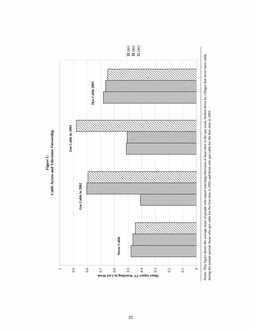
Figu

re 1

: C

able

Acc

ess a

nd T

elev

isio

n V

iew

ersh

ip

0

0.1

0.2

0.3

0.4

0.5

0.6

0.7

0.8

0.91

Share report TV Watching in Last Week

2001

2002

2003

Has

Cab

le 2

001

Got

Cab

le in

200

2

Got

Cab

le in

200

3

Not

es: T

his f

igur

e sh

ows t

he a

vera

ge sh

are

of p

eopl

e w

ho re

port

wat

chin

g te

levi

sion

at l

east

onc

e in

the

last

wee

k, b

roke

n do

wn

by v

illag

es th

at n

ever

hav

e ca

ble

durin

g th

e sa

mpl

e pe

riod,

thos

e w

ho g

ot c

able

for t

he fi

rst t

ime

in 2

002

and

thos

e w

ho g

ot c

able

for t

he fi

rst t

ime

in 2

003.

Nev

er C

able

32

Figu

re 2

a:

Cab

le A

cces

s and

Fem

ale

Aut

onom

y

-0.3

-0.2

-0.10

0.1

0.2

0.3

0.4

0.5

Need for Permission for Various Activities, Decision Making Ability

2001

2002

2003

Got

Cab

le in

200

2G

ot C

able

in 2

003

Nev

er C

able

Not

es: T

his f

igur

e sh

ows t

he fi

rst p

rinci

pal c

ompo

nent

of s

ix m

easu

res o

f fem

ale

auto

nom

y, b

roke

n do

wn

by v

illag

es w

ith n

o ch

ange

in c

able

stat

us d

urin

g th

e sa

mpl

e pe

riod,

th

ose

who

got

cab

le fo

r the

firs

t tim

e in

200

2 an

d th

ose

who

got

cab

le fo

r the

firs

t tim

e in

200

3.

Alw

ays C

able

33

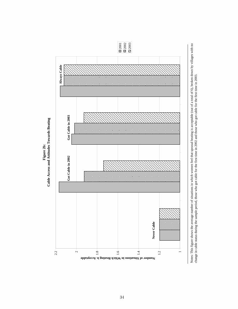
Figu

re 2

b:

Cab

le A

cces

s and

Att

itude

s Tow

ards

Bea

ting

1

1.2

1.4

1.6

1.82

2.2

Number of Situations in Which Beating is Acceptable

2001

2002

2003

Got

Cab

le in

200

2G

ot C

able

in 2

003

Nev

er C

able

Not

es: T

his f

igur

e sh

ows t

he a

vera

ge n

umbe

r of s

ituat

ions

in w

hich

wom

en fe

el th

at sp

ousa

l bea

ting

is a

ccep

tabl

e (o

ut o

f a to

tal o

f 6),

brok

en d

own

by v

illag

es w

ith n

o ch

ange

in c

able

stat

us d

urin

g th

e sa

mpl

e pe

riod,

thos

e w

ho g

ot c

able

for t

he fi

rst t

ime

in 2

002

and

thos

e w

ho g

ot c

able

for t

he fi

rst t

ime

in 2

003.

Alw

ays C

able

34

Figu

re 2

c:

Cab

le A

cces

s and

Son

Pre

fere

nce

0.3

0.350.

4

0.450.

5

0.550.

6

0.65

Report Want Next Child to be a Boy

2001

2002

2003

Got

Cab

le in

200

2

Got

Cab

le in

200

3

Nev

er C

able

Not

es: T

his f

igur

e sh

ows t

he sh

are

of w

omen

who

wan

t a m

ale

child

at t

heir

next

birt

h, c

ondi

tiona

l on

wan

ting

anot

her c

hild

, bro

ken

dow

n by

vill

ages

with

no

chan

ge

in c

able

stat

us d

urin

g th

e sa

mpl

e pe

riod,

thos

e w

ho g

ot c

able

for t

he fi

rst t

ime

in 2

002

and

thos

e w

ho g

ot c

able

for t

he fi

rst t

ime

in 2

003.

Alw

ays C

able

35

Table 1. Summary Statistics on Cable Availability

Panel A: Cable Availability by Survey RoundYear Number of Villages with Cable2001 652002 752003 86

Not During Survey 94Panel B: Cable Availability in 2001 by State

State Share of Villages with CableBihar 7.5%Delhi 97.1%Goa 60%

Haryana 17.5%Tamil Nadu 77.5%

Notes: This table shows summary statistics on cable availability, either over time or acrossstate in the first sample year.

36

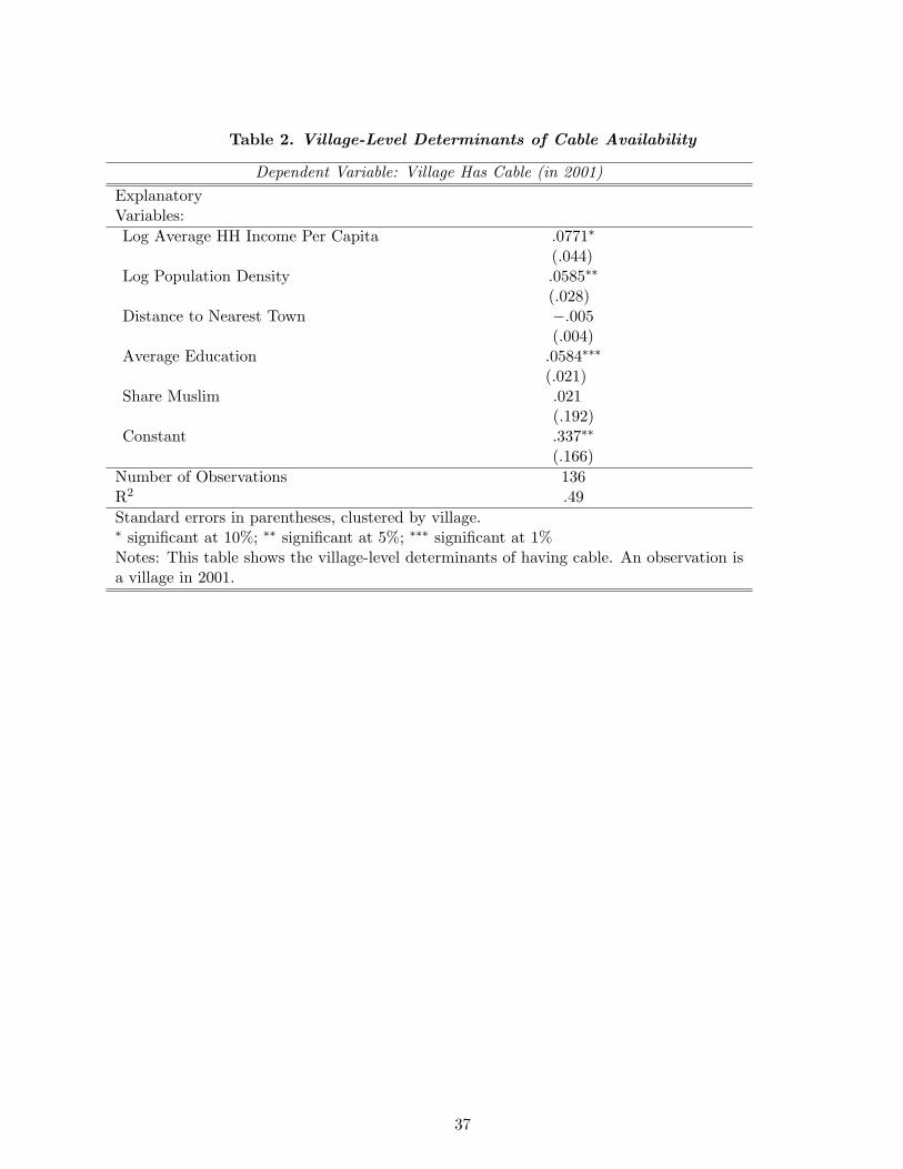
Table 2. Village-Level Determinants of Cable Availability

Dependent Variable: Village Has Cable (in 2001)ExplanatoryVariables:Log Average HH Income Per Capita .0771∗

(.044)Log Population Density .0585∗∗

(.028)Distance to Nearest Town −.005

(.004)Average Education .0584∗∗∗

(.021)Share Muslim .021

(.192)Constant .337∗∗

(.166)Number of Observations 136R2 .49Standard errors in parentheses, clustered by village.∗ significant at 10%; ∗∗ significant at 5%; ∗∗∗ significant at 1%Notes: This table shows the village-level determinants of having cable. An observation isa village in 2001.

37

Table 3. Summary Statistics on Dependent Variables

Panel A: Gender AttitudesMean Standard Deviation # Obs

Attitudes towards beatingBeating ever acceptable 0.621 0.485 9159# of situations beating is ac-ceptable

1.61 1.73 9159

Husband may hit if:Unfaithful 0.244 0.429 9159Family doesn’t give money 0.204 0.403 9159Show disrespect 0.308 0.461 9159Go out without telling 0.306 0.461 9159Neglect children 0.336 0.472 9159Bad cook 0.215 0.411 9159Autonomy: Respondent can make decisions aboutHealth care 0.566 0.495 9159Purchases 0.556 0.496 9159Visits to family/friends 0.549 0.497 9159Autonomy: Respondent needs permission to visitMarket 0.561 0.537 9159Friends 0.675 0.496 9159Autonomy: MoneyResp. keeps own money 0.739 0.438 9159Son PreferenceWant next child to be a boy 0.549 0.497 2165

Panel B: Fertility and EducationMean Standard Deviation # Obs

Average # children 1.107 1.78 8208Change in # children 0.142 0.352 5472Share in school, age 6-14 0.743 0.436 8587Share dropout, ages 6-14 0.135 0.341 4455Notes: This table shows summary statistics for the dependent variables used in the paper.All of the autonomy, beating attitudes and son preference measures are binary. Sonpreference is only asked of women who report wanting more children.

38

Table 4. Correlations Between Outcomes and Demographics

Dependent Var.: Autonomy Beating Attitudes Son Preference # Children In school (6-14)ExplanatoryVariables:Rural Area -0.137∗∗ 0.7460∗∗∗ 0.0622 0.220∗∗∗ -0.0542∗∗∗

Education 0.0335∗∗∗ -0.0461∗∗∗ -0.0316∗∗∗ -0.135∗∗∗ 0.047∗∗∗

Log HH Income PC 0.0190∗∗ -0.0424∗∗∗ -0.0176∗∗∗ 0.0801∗∗∗ 0.0171∗∗∗

Age 0.035∗∗∗ 0.006∗ -0.002 0.113∗∗∗ N/AMuslim -0.485∗∗∗ -0.529∗∗∗ 0.157∗∗∗ 1.052∗∗∗ -0.137∗∗∗

Hindu -0.0318 0.195∗∗ 0.0511 -0.3907∗∗∗ 0.0478∗∗

Sched. Caste -0.130 -0.114 -0.134 0.3710∗∗∗ 0.017∗ significant at 10%; ∗∗ significant at 5%; ∗∗∗ significant at 1%Notes: This table reports the coefficients from regressions of each outcome variable (au-tonomy, beating attitudes, son preference, number of children and whether a child is inschool) on demographics. Each cell represents a separate regression, with no other controlsother than that demographic characteristic (and a constant).

39

Table 5. Cable Television and Attitudes, OLS Regression

Panel A: Limited Controls

Dependent Variable: Autonomy Attitudes Son Preference

ExplanatoryVariables:

Village Has Cable .6166∗∗∗

(.075).4593∗∗∗

(.12)−.2896∗∗∗

(.046)

Constant −.318∗∗∗

(.049)1.424∗∗∗

(.08).669∗∗∗

(.026)

Year FE YES YES YESNumber of Observations 9159 9159 1998R2 .05 .02 .08

Panel B: With Controls

Dependent Variable: Autonomy Attitudes Son Preference

ExplanatoryVariables:

Village Has Cable .1215∗

(.063).0148(.095)

−.0634∗∗

(.031)

Log HH Income per Capita .0100(.008)

−.0007(.01)

−.0111∗

(.006)

Education .0154∗∗∗

(.006)−.0649∗∗∗

(.007)−.0155∗∗∗

(.004)

Age .0306∗∗∗

(.003)−.0047(.003)

.0056∗

(.003)

Hindu −.1478(.134)

−.2005(.165)

.0345(.093)

Muslim −.2879∗

(.175)−.5614∗∗

(.22).0649(.105)

SC/ST .0392(.151)

−.5504∗∗∗

(.189)−.1799∗

(.098)

Rural −.1685(.185)

−.0393(.192)

−.0487(.105)

Constant −.871∗∗∗

(.258)2.274∗∗∗

(.311).587∗∗∗

(.171)

Year FE YES YES YESState FE YES YES YESNumber of Observations 9159 9159 1998R2 .16 .22 .22

Standard errors in parentheses, clustered by village∗ significant at 10%; ∗∗ significant at 5%; ∗∗∗ significant at 1%Notes: This table shows OLS regressions of outcomes on cable access. Column 1 reports the effect onthe first principal component of a number of autonomy measures (does the woman make decisionsabout her health, purchases or visits, does she need permission to go to the market or visit herfamily and can she keep her own money). Column 2 reports the effect on attitudes towards beating(the sum of the number of situations in which the woman reports spousal beating is acceptable).Column 3 reports the effect on son preference - the share of women who report wanting their nextchild to be a boy (conditional on wanting another child).

40

Table 6. Cable television and Attitudes, Fixed Effect Regressions

Dependent Variable: Autonomy Attitudes Son PreferenceExplanatoryVariables:Village Has Cable .1896∗∗∗

(.044)−.1880∗∗∗

(.066)−.1214∗∗∗

(.037)Year=2002 −.0068

(.036).0337(.044)

.021(.022)

Year=2003 .0573(.035)

.0252(.056)

.0326(.027)

Log HH Income Per capita .0038(.006)

−.0066(.007)

−.0038(.003)

Income × Year=2002 .0071(.006)

−.0056(.007)

−.0027(.003)

Income × Year=2003 −.0052(.005)

−.0061(.011)

−.0031(.004)

Education × Year=2002 −.0024(.004)

−.0036(.005)

−.0005(.002)

Education × Year=2003 .0021(.003)

−.0019(.005)

−.0002(.002)

Constant −.14∗∗∗

(.038)1.76∗∗∗

(.053).619∗∗∗

(.025)

Individual FE YES YES YESNumber of Observations 9159 9159 1998

R2 .91 .86 .93Standard errors in parentheses, clustered by village∗ significant at 10%; ∗∗ significant at 5%; ∗∗∗ significant at 1%Notes: This table shows individual-level regressions of our dependent variables on cableaccess. Column 1 reports the effect on the first principal component of a number ofautonomy measures (does the woman make decisions about her health, purchases or visits,does she need permission to go to the market or visit her family and can she keep herown money). Column 2 reports the effect on attitudes towards beating (the sum of thenumber of situations in which the woman reports spousal beating is acceptable). Column3 reports the effect on son preference - the share of women who report wanting their nextchild to be a boy (conditional on wanting another child).

41

Table 7. Effect of Cable: Matching Results

Panel A: Attitudes, Autonomy and Son PreferenceDependent Variable: Coefficient, SATE Standard ErrorAutonomy 0.1601∗∗∗ 0.0532Beating Attitudes -0.1737∗∗ 0.0837Son Preference -0.1311∗∗∗ 0.0541Panel B: Education, Determinants of Being Enrolled/Dropping OutGroup: Coefficient, SATE Standard ErrorGirls, Ages 6-10 0.0728∗ 0.0406Boys, Ages 6-10 -0.0296 0.0614Girls, Ages 11-14 -0.0540 0.0692Boys, Ages 11-14 0.0655 0.0532

Panel C: Fertility, Change in Number of ChildrenGroup: Coefficient, SATE Standard ErrorFull Sample -0.0806∗∗ 0.0389Age <35 -0.1205∗ 0.0658∗ significant at 10%; ∗∗ significant at 5%; ∗∗∗ significant at 1%Notes: This table shows the effect of cable on outcomes, based on matchingvillages based on ex-ante characteristics and then comparing the subsequentchanges in outcomes across villages that do and do not get access to cable. Inall cases we match to the 4 nearest neighbor villages. The matching procedureis described in more detail in the empirical strategy section.

42

Table 8. Share of Urban Rural Difference Explained by Television

Outcome Urban Mean Rural Mean, No television Effect of television Share Explained

Autonomy 0.120 -0.324 0.1896 42.6%Beating 0.964 1.378 -0.1888 45.5%Son Preference 0.500 0.6728 -0.1214 70.1%Notes: Table displays calculations of the share of the urban-rural difference in each dependent variablethat is made up by the introduction of television. The urban area is Delhi. The rural mean is amongthe rural areas that do not have cable access. Share explained is simply the effect size (column 4)divided by the difference between Column 2 and Column 3.

43

Table 9. Cable Television, Education and Fertility, OLS Regression

Dependent Variable: Enrolled in School Change in # KidsGirls, 6-14 Boys, 6-14 (including Current Pregnancies)

ExplanatoryVariables:Village Has Cable .0553∗

(.032).0441∗

(.024)−.0313∗∗∗

(.011)Log HH Income Per Capita .0151∗∗∗

(.004).0113∗∗∗

(.004).0012(.002)

Household Ave. Adult Educ. .0492∗∗∗

(.009).025∗∗∗

(.008)Child Age in 2001 −.03∗∗∗

(.004)−.014∗∗∗

(.004)Hindu −.045

(.046)−.0495(.044)

−.0209(.018)

Muslim −.1486∗∗

(.067)−.1429∗∗

(.058).0587∗∗

(.026)SC/ST .0875

(.087)−.0743(.068)

.0234(.013)

Rural .0153(.037)

.0519(.037)

−.018(.014)

Education .0013(.001)

Age −.0159∗∗∗

(.001)Pregnant Last Year −.2139∗∗∗

(.013)Constant .829∗∗∗

(.085).809∗∗∗

(.094).725∗∗∗

(.035)Year FE YES YES YESNumber of Observations 4594 4988 5423R2 .09 .04 .15Standard errors in parentheses, clustered by village∗ significant at 10%; ∗∗ significant at 5%; ∗∗∗ significant at 1%Notes: This table shows OLS regressions of fertility and education on cable access.Columns 1 and 2 show the effect of cable on children’s school enrollment, for girls andboys respectively. Column 3 shows the effect on fertility.

44

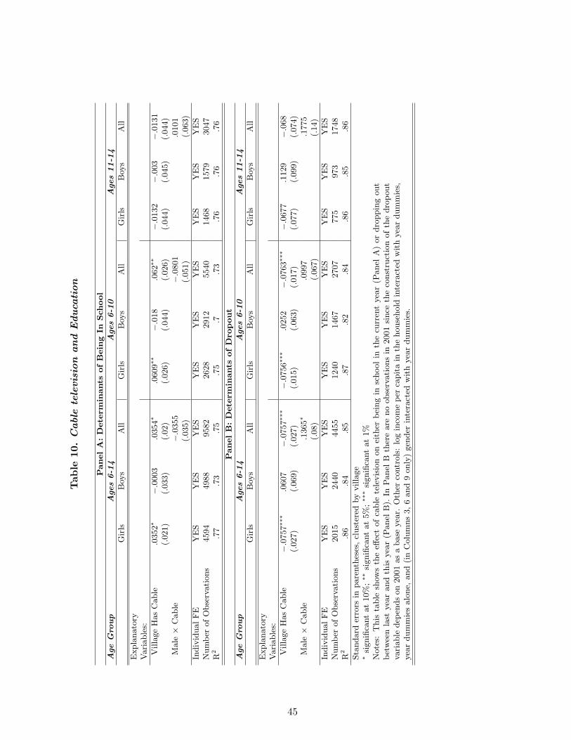
Tab

le10

.C

able

tele

vis

ion

an

dE

du

cati

on

PanelA

:D

ete

rmin

ants

ofB

ein

gIn

Sch

ool

Age

Gro

up

Ages

6-1

4A

ges

6-1

0A

ges

11-1

4

Gir

lsB

oys

All

Gir

lsB

oys

All

Gir

lsB

oys

All

Expla

nato

ryV

ari

able

s:

Villa

ge

Has

Cable

.0352∗

(.021)

−.0

003

(.033)

.0354∗

(.02)

.0609∗∗

(.026)

−.0

18

(.044)

.062∗∗

(.026)

−.0

132

(.044)

−.0

03

(.045)

−.0

131

(.044)

Male×

Cable

−.0

355

(.035)

−.0

801

(.051)

.0101

(.063)

Indiv

idual

FE

YE

SY

ES

YE

SY

ES

YE

SY

ES

YE

SY

ES

YE

SN

um

ber

of

Obse

rvati

ons

4594

4988

9582

2628

2912

5540

1468

1579

3047

R2

.77

.73

.75

.75

.7.7

3.7

6.7

6.7

6

PanelB

:D

ete

rmin

ants

ofD

ropout

Age

Gro

up

Ages

6-1

4A

ges

6-1

0A

ges

11-1

4

Gir

lsB

oys

All

Gir

lsB

oys

All

Gir

lsB

oys

All

Expla

nato

ryV

ari

able

s:

Villa

ge

Has

Cable

−.0

757∗∗

∗

(.027)

.0607

(.069)

−.0

757∗∗

∗

(.027)

−.0

756∗∗

∗

(.015)

.0252

(.063)

−.0

763∗∗

∗

(.017)

−.0

677

(.077)

.1129

(.099)

−.0

68

(.074)

Male×

Cable

.1365∗

(.08)

.0997

(.067)

.1775

(.14)

Indiv

idual

FE

YE

SY

ES

YE

SY

ES

YE

SY

ES

YE

SY

ES

YE

SN

um

ber

of

Obse

rvati

ons

2015

2440

4455

1240

1467

2707

775

973

1748

R2

.86

.84

.85

.87

.82

.84

.86

.85

.86

Sta

ndard

erro

rsin

pare

nth

eses

,cl

ust

ered

by

villa

ge

∗si

gnifi

cant

at

10%

;∗∗

signifi

cant

at

5%

;∗∗

∗si

gnifi

cant

at

1%

Note

s:T

his

table

show

sth

eeff

ect

of

cable

tele

vis

ion

on

eith

erb

eing

insc

hool

inth

ecu

rren

tyea

r(P

anel

A)

or

dro

ppin

gout

bet

wee

nla

styea

rand

this

yea

r(P

anel

B).

InP

anel

Bth

ere

are

no

obse

rvati

ons

in2001

since

the

const

ruct

ion

of

the

dro

pout

vari

able

dep

ends

on

2001

as

abase

yea

r.O

ther

contr

ols

:lo

gin

com

ep

erca

pit

ain

the

house

hold

inte

ract

edw

ith

yea

rdum

mie

s,yea

rdum

mie

salo

ne,

and

(in

Colu

mns

3,

6and

9only

)gen

der

inte

ract

edw

ith

yea

rdum

mie

s.

45

Table 11. Cable Television and Fertility

Dependent Variable: Change in # Kids Wants More Children(Including Current Pregnancies)(1) (2) (3) (4)All Age <=35 Age>35 Age<=35

ExplanatoryVariables:Village Has Cable −.087∗∗∗

(.021)−.1436∗∗∗

(.038)−.0007(.009)

.0481(.044)

Pregnant at Last Survey −.6077∗∗∗

(.025)−.6164∗∗∗

(.027)−.5171∗∗∗

(.082)−.0284(.022)

Log HH Income PC −.0011(.011)

.002(.017)

−.0082∗

(.005)−.0063(.008)

Year=2003 .0695∗∗

(.029).115∗∗

(.046).0017(.015)

.0149(.035)

Income × Year=2003 −.0128∗∗

(.006)−.02∗∗

(.009)−.0019(.003)

−.0108(.007)

Education × Year=2003 −.004∗

(.002)−.0063∗∗

(.003)−.0001(.001)

−.001(.002)

constant .241∗∗∗

(.044).35∗∗∗

(.067).063∗∗∗

(.02).489∗∗∗

(.038)Individual FE YES YES YES YESNumber of Observations 5423 3423 2000 2251R2 .57 .53 .61 .87Standard errors in parentheses, clustered by village∗ significant at 10%; ∗∗ significant at 5%; ∗∗∗ significant at 1%Notes: This table shows the effect of cable television on the change in number of childrenbetween years (Columns 1 through 3) and reported desire for more children (Column 4). Ifan individual is pregnant in year t, that is counted as an increase in a child between yeart − 1 and year t. The dataset includes two observations per person, one in 2002 and one in2003 since we are using changes, so we need 2001 as the first comparison year. Column 1includes all women, Columns 2 and 4 are limited to women under 35 and Column 3 is limitedto women over 35.

46

Table 12. Trends in Attitudes and Cable Adoption

Dependent Variable: Village Adopted Cable between 2002 and 2003ExplanatoryVariables:Change in Autonomy 2001-2002 −.172

(.224)Change in Beating Att. 2001-2002 −.0049

(.143)Change in Sex Preference 2001-2002 −.0279

(.141)Log Ave HH Income Per Capita −.1316

(.089)−.1408(.089)

−.1418(.091)

Education .0453∗

(.026).0466∗

(.026).0459∗

(.027)

Hindu .0262(.569)

.0445(.574)

.0561(.577)

Muslim .0654(.595)

.1012(.601)

.1094(.601)

Christian 1.55∗∗

(.763)1.6222∗∗

(.765)1.6619∗∗

(.785)

Family Size −.1011∗

(.055)−.097∗

(.055)−.0948∗

(.056)

Main Crop is Rice −.0808(.081)

−.0907(.08)

−.0903(.082)

Distance to Nearest Town .0051(.004)

.0052(.004)

.0053(.004)

constant 1.516(1.015)

1.526(1.02)

1.507(1.035)

Number of Observations 79 79 78R2 .19 .18 .18

Standard errors in parentheses∗ significant at 10%; ∗∗ significant at 5%; ∗∗∗ significant at 1%Notes: This table examines the predictors of getting cable television between 2002and 2003 and tests for whether trends in the gender attitude variables are importantpredictors of television introduction. The data are for 2002 and is limited to villagesthat did not have cable in 2002. The dependent variable is equal to 1 if the villagegot cable between 2002 and 2003 and 0 if they did not. The independent variableson attitudes are changes in village level averages between 2001 and 2002.

47

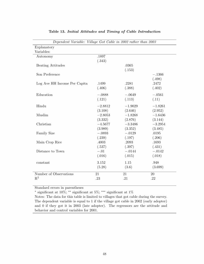
Table 13. Initial Attitudes and Timing of Cable Introduction

Dependent Variable: Village Got Cable in 2002 rather than 2003ExplanatoryVariables:Autonomy .1897

(.343)Beating Attitudes .0365

(.153)Son Preference −.1366

(.498)Log Ave HH Income Per Capita .1499

(.406).2281(.388)

.2472(.402)

Education −.0888(.121)

−.0649(.113)

−.0561(.11)

Hindu −2.8812(3.108)

−1.9029(2.646)

−1.8261(2.952)

Muslim −2.8053(3.332)

−1.8268(2.876)

−1.6436(3.144)

Christian −4.5677(3.989)

−3.3486(3.352)

−3.2954(3.485)

Family Size −.0893(.239)

−.0129(.197)

.0195(.206)

Main Crop Rice .4003(.537)

.2093(.397)

.1693(.431)

Distance to Town −.01(.016)

−.0144(.015)

−.0142(.018)

constant 3.152(5.28)

1.15(3.6)

.948(3.699)

Number of Observations 21 21 20R2 .23 .21 .22

Standard errors in parentheses∗ significant at 10%; ∗∗ significant at 5%; ∗∗∗ significant at 1%Notes: The data for this table is limited to villages that got cable during the survey.The dependent variable is equal to 1 if the village got cable in 2002 (early adopter)and 0 if they got it in 2003 (late adopter). The regressors are the attitude andbehavior and control variables for 2001.

48

Table 14. Trends in Attitudes for “Early” Adopters

Changes 2001 to 2002 for Adopters 2-3 Months After 2002 SurveyDependent Variable: Autonomy Beating Attitudes2001 -0.265 1.7872002 -0.381 1.9102003 -0.185 1.785

Changes 2002 to 2003 for Adopters 2-3 Months After 2003 SurveyDependent Variable: Autonomy Beating Attitudes2001 -0.070 1.9892002 0.036 1.9842003 -0.114 2.105Notes: This table shows trends in autonomy and beating attitudes for villages that adoptcable within 2-3 months after the previous survey. These “early” adopters would have theknowledge of getting cable at the previous survey. Looking at the changes therefore is atest for pre-existing trends.

49

Table 15. Mechanism Test: Effect Breakdown by Initial Attitudes

Dependent Variable: Autonomy Beating Son PreferenceInitial State Low High High Low High LowExplanatoryVariables:Village Has Cable .2316∗∗∗

(.051).1408∗

(.077)−.2559∗∗

(.1)−.0766(.085)

−.2106∗∗∗

(.047)−.0098(.027)

Log HH Income PC .009(.008)

−.0044(.009)

.0054(.007)

−.0164(.011)

−.0022(.004)

−.0051(.005)

year=2002 −.0239(.048)

.0067(.049)

.0936(.058)

−.0404(.073)

.0181(.035)

.0469∗

(.025)year=2003 .0285

(.055).0801∗∗

(.039)−.0347(.05)

.0945(.094)

.0327(.035)

.0149(.032)

Educ × Year=2002 −.0019(.004)

−.002(.005)

−.0014(.007)

−.0059(.006)

−.0046(.005)

−.0019(.003)

Educ × Year=2003 .0061(.005)

−.0004(.005)

−.0005(.006)

−.0023(.007)

−.0068(.005)

.0012(.002)

Income × Year=2002 .0115(.009)

.0031(.007)

−.0178∗∗

(.008).0087(.012)

−.0037(.005)

−.0023(.002)

Income × Year=2003 −.0005(.009)

−.0092(.006)

−.002(.009)

−.0126(.016)

−.0022(.006)

.0004(.004)

constant −.676∗∗∗

(.044).44∗∗∗

(.077)2.52∗∗∗

(.084).997∗∗∗

(.074).858∗∗∗

(.026).321∗∗∗

(.03)Individual FE YES YES YES YES YES YESNumber of Obs 4599 4560 4560 4599 1003 993R2 .89 .9 .88 .73 .88 .93Standard errors in parentheses, clustered by village∗ significant at 10%; ∗∗ significant at 5%; ∗∗∗ significant at 1%Notes: This table shows the effect of cable television on individual-level attitudes, broken down by the averageinitial attitude level in the village. Columns 1 and 2 break down based on autonomy, Columns 3 and 4 basedon beating attitudes and Columns 5 and 6 based on son preference.

50

Appendix Tables

Appendix Table 1. Effect of Cable on Beating Attitude, Autonomy Components

Effect of Cable Standard ErrorAttitudes towards beating: Husband May Hit ifUnfaithful 0.0103 0.0148Family doesn’t give money -0.0481∗∗ 0.0196Show Disrespect -0.0262 0.0231Go out without telling 0.0054 0.0119Neglect Children -0.0543∗∗ 0.0206Bad Cook -0.0750∗∗∗ 0.0259Autonomy: Respondent can make decisions aboutHealth Care 0.0212 0.0244Purchases 0.0894∗∗∗ 0.0258Visits to Family/Friends -0.0048 0.0273Autonomy: Respondent needs permission to visitMarket -0.0585∗∗∗ 0.0201Friends -0.0371∗∗∗ 0.0111Autonomy: MoneyResp. keeps own Money 0.0352∗∗∗ 0.0128

∗ significant at 10%; ∗∗ significant at 5%; ∗∗∗ significant at 1%Notes: This table shows the effect of cable access on the components ofthe autonomy and beating measure. All outcomes are binary.

51

Appendix Table 2. Effect of Cable by Age, Education

Panel A: Breakdown by AgeDependent Variable: Autonomy Attitudes Son Preference

Younger0.1170∗

(.0605)−0.1723∗∗

(.0724)N/A

Older0.2691∗∗∗

(.0639)−0.2037∗∗

(.0951)N/A

Panel B: Breakdown by EducationDependent Variable: Autonomy Attitudes Son Preference

Less Educated0.0551(.0399)

−0.0858(.0824)

−0.0750(.0487)

More Educated0.3888∗∗∗

(.0825)−0.3369∗∗∗

(.0658)−0.1652∗∗∗

(.0599)∗ significant at 10%; ∗∗ significant at 5%; ∗∗∗ significant at 1%Notes: This table shows the effects of cable broken down by age and education. Inboth cases, the dataset is split in half, so the younger group is the youngest half of thedataset and the less educated group is the bottom half in terms of years of education.In Panel A, the effects on son preference are not shown because this questions isonly asked to younger women who are still planning to have more children.

52

Appendix Table 3. Effect of TV Watching, Instrumented with Cable Access

Effect of Watching TV (IV Estimate) Standard Error

Attitudes, Autonomy and Son PreferenceAutonomy 0.4841∗∗∗ 0.1352Beating Attitudes -0.4799∗∗∗ 0.1682Son Preference -0.3035∗∗∗ 0.1053

FertilityChange in # of Children, All -0.2051∗∗∗ 0.0586Change in # of Children, Under 35 -0.3482∗∗∗ 0.1152Change in # of Children, Over 35 -0.0016 0.0209

EducationIn School, Girls 6-14 0.0700 0.0459In School, Boys 6-14 -0.0077 0.0967Dropout, Girls 6-14 -0.1468∗∗∗ 0.0521Dropout, Boys 6-14 0.1918 0.2147

∗ significant at 10%; ∗∗ significant at 5%; ∗∗∗ significant at 1%Notes: This table shows regressions of the outcome variables on whether the surveyed individualreports watching television in the last week. This measure of watching is instrumented with cableaccess. The regressions include the same controls as in the non-IV regressions in the text – income,year dummies, income and education interacted with the year dummies.

53