The positive and negative effects of the mining boom – A technical paper

Tien Duc Pham, Geoff Bailey and Ray Spurr

1

Acknowledgments

The authors would like to thank Professor Philip Adams at Monash University and Dr. Hom Pant at the Australian Bureau of Agricultural and Resource Economics and Sciences for their technical advice during this project.

AuthorsTien Duc Pham (Tourism Research Australia)Geoff Bailey (Tourism Research Australia)Ray Spurr (University of New South Wales)

Editing Darlene Silec (Tourism Research Australia)

ISBN 978-1-922106-98-8 (PDF)978-1-922106-99-5 (Word)

Tourism Research AustraliaDepartment of Resources, Energy and TourismGPO Box 1564Canberra ACT 2601ABN 46 252 861 927

Email: tourism.research@ret.gov.au Web: www.tra.gov.au

Publication date: June 2013

This work is licensed under a Creative Commons Attribution   3.0 Australia licence . To the extent that copyright subsists in third party quotes and diagrams it remains with the original owner and permission may be required to reuse the material.

This work should be attributed as The positive and negative effects of the mining boom – A technical paper, Tourism Research Australia, Canberra.

2

Inquiries regarding the licence and any use of work by Tourism Research Australia are welcome at tourism.research@ret.gov.au

Introduction

This paper supplements the previous TRA mining boom report (Pham, Bailey and Marshall, 2013) by elaborating on the technical aspects of the modelling involved in the report. It is intended to facilitate a clearer understanding of the drivers of the modelling results reflected in those reports. It provides a more detailed explanation of the assumptions used in the modelling and the analysis of results than that provided in the previous reports.

From a policy perspective, the objective of the modelling was to analyse potential impacts, both positive and negative, of the mining boom on the economies and tourism sectors of Australia and its states and territories. The mining boom is defined as comprising the increases in mining exports from Queensland, Western Australia and the Northern Territory. One special characteristic of the mining boom was an increase in Fly-In/Fly-Out (FIFO)1 employment in the mining areas, as the mining industry brought workers from outside regions to the mining areas. The consequence of FIFO was increased demand for air transport and accommodation, which had impacts on the local tourism sectors. The additional demand generated by FIFO employees adds a significant complication to the effects of the mining boom on tourism.

The modelling was devised to decompose the economic impacts of the mining boom through three stages. In the first stage, the modelling focuses on a base case that captures the mining boom with some realistic conditions of FIFO and a constrained supply of accommodation and air transport services. In the second stage, the effect of FIFO on the economy and tourism sectors is measured more explicitly. In the final stage, the modelling measures the potential effects when supply of both air transport and accommodation sectors increases capacity to the extent necessary to serve the FIFO demand.

Modelling approach

The Computable General Equilibrium (CGE) tourism model used in preparing these reports is explained in greater detail in Appendix 1 (see also Pham and Dwyer in Tisdell, 2013). It is important to note that the modelling version adopted, MMRF-Tour, captures only non-business tourism for interstate, intrastate, inbound visitors, and outbound travellers. Business tourism is embedded within the individual cost structures of the industries within the model database. For the purposes of the modelling, however, the demand generated by the mining FIFO employees is separately identified and modelled specifically as increases in usage of air transport and accommodation by the mining sectors.

1 Drive-in/Drive-out (DIDO) is also included but for simplicity FIFO is used for both.

3

A base case scenario is used to reflect the impacts of the mining boom and its associated FIFO activity on the economy generally and on the tourism sectors specifically. Two additional simulations are used in conjunction with the base case to measure the effects of FIFO and the effects of additional investment injected into accommodation and air transport to satisfy FIFO demand. The first simulation captures the effect of high demand for accommodation and air transport required by the mining sector for FIFO activity under existing supply constraints applying in these two sectors. The accommodation and air transport sectors are assumed to be unable to respond quickly enough to the rapid increase in demand. This reflects the reality of a rapid expansion of FIFO demand crowding out the tourism services (in this case aviation and accommodation) available to service leisure tourism activity more generally in the affected regions.

The second simulation investigates the impacts when accommodation and air transport sectors have responded fully to the additional FIFO demand, expanding their services level by increasing their investment to build up capital stocks. This step was aimed at measuring the benefits from the spill-over effect of increased supply in the accommodation and air transport sectors on leisure tourism.

The mining boom dates back to 2005. There was a subdued period during the global financial crisis, before it picked up again over the period 2010–12. The model database was for 2004–05, suitable for the impacts of the mining boom to be assessed on an average annual basis over the period 2004–05 to 2011–12.

The mining boom was mainly driven by strong demand for coal, iron ore and other non-ferrous ores from overseas countries such as China and India. Because the existing model database contains separate data for only coal, oil and gas—and all other mining outputs are aggregated into a single industry defined as “other mining”—, the modelling explicitly examined coal exports from Queensland and exports of other mining from Western Australia and Northern Territory. The inclusion of Northern Territory is to ensure that the relative importance of mining in Northern Territory economy was factored into the analysis, even though total exports of other mining from Northern Territory are no larger than those from some other states.

Over the period 2004–05 to 2011–12, black coal exports from Queensland were estimated to increase by 5% on average, while other mining is estimated to have increased by 12% from Western Australia2 and 10% from Northern Territory3.

Increases in demand for accommodation and air transport generated by FIFO activity in Queensland and Western Australia were separately estimated for the purpose of the modelling. Drawing on comparison of Input-Output data on input usage by mining sectors between 2004–05 and 2008–09 (ABS, 2008 and 2012), it was assumed that both black coal and other mining in Queensland and Western Australia increased their demand for both

2 We acknowledge the assistance of the Bureau of Resources and Energy Economics in the development of these estimates.3 The assistance of Tourism Northern Territory in the development of these estimates is acknowledged.

4

accommodation and air transport services by 300%, while other mining in Northern Territory increased its demand for accommodation and air transport by 100%. The lower increase by FIFO in Northern Territory reflects its already well-established reliance on FIFOs to source its mining workforce at the time that the mining boom gained momentum in the mid-2000s.

The modelling steps

The MMRF-Tour model was used in a long-run comparative static mode to assess the economic impacts of the mining boom. Results of a comparative static simulation represent the impacts on an annual average basis.

The modelling consists of three simulations which are described in Figure 1 with corresponding shocks for each simulation. The first simulation examines the effects of the mining boom alone. Shocks to exports of coal and other mining in the three mining states determine the requirement of inputs used by the mining sectors, including labour, capital and intermediate inputs. However, the structure of the model could only raise the demand for accommodation and air transport in the same proportion as changes in mining outputs. The demand for accommodation and air transport in the presence of FIFO is not captured by the theory of the model. Therefore, without a direct control of the demand shocks to reflect FIFO in Simulation 1, the demand for accommodation and air transport services in this first simulation represents a case of a mining boom without FIFO. Consequently, the output levels of accommodation and air transport services are used as the benchmark level without the FIFO effect.

Simulation 2 presents the actual mining boom situation in the three states where demands for accommodation and air transport services are also assumed to increase strongly due to FIFO demand. The supply of these services is kept at the benchmark level in Simulation 1 to reflect the reality that these sectors could not expand their capacity quickly enough to satisfy FIFO demand. Results of Simulation 2 are presented as the base case result for the mining boom impacts.

In Simulation 3, the assumption of constrained output levels of accommodation and air transport is relaxed. These two sectors are now assumed to respond fully to the demand imposed by FIFO activity by increasing investment to expand their capacity. While the actual extent to which these sectors expand capacity to meet the increase in FIFO may not be the same as the level depicted by the model, the results in Simulation 3 indicate the potential impacts when the two sectors have responded fully to the new market conditions.

5

Figure 2: Simulation procedure

While results of Simulation 2 are used to portray the impacts of the mining boom on the regional (state) economies and tourism sectors, the difference in results between Simulation 2 and Simulation 1 is used to show the specific impacts of FIFO activity on the tourism sectors and state economies. Similarly, the difference in results between Simulation 3 and Simulation 2 is used to show the potential impacts of investment in accommodation and air transport (as a result of expansion of their supply capacity) on the state economies and tourism sectors.

Results of Simulation 2 are presented as annual average percentage changes in a typical year in the timeframe 2004–05 to 2011–12. In the following sections, explanation and analysis of Simulation 2 are presented first.

The impacts of FIFO and of capacity expansion of accommodation and air transport services on the regional economies and tourism sectors will be presented as percentage point changes, i.e. the difference in result between two associate simulations.

Simulation closures

As is usual in CGE modelling, the results of the modelling are influenced by the choice of closure, in which variables are set either exogenously or endogenously. While results of endogenous variables are determined by the model, exogenous variables are often set at zero to reflect the absence of any changes before and after the shocks.

In all three simulations, the model was set in a long run environment. In a typical long run comparative static simulation, the supply of capital is assumed to be perfectly elastic. This implies that capital is not constrained by the supply from the domestic source only. Capital could also be supplied from the rest of the world at a given rate of return determined outside of the economy.

6

Simulation 1(1) Mining export shocksThis determines output levels of accommodation and air transport services

Simulation 2(1) Mining export shocks(2) Additional FIFO demand shocks for accommodation and air transport (3) Re-use output levels of accommodation and air transport from Simulation 1

Simulation 3(1) Mining export shocks (2) The same additional FIFO demand shocks for accommodation and air transport as in Simulation 2

For the labour market, it is assumed that national employment is fixed while the real wage adjusts to clear the labour market. This implies that for a given level of labour supply in the economy, all of those who wish to work will be willing to accept a market real wage rate in order to find a job. This real wage rate is from the consumer point of view, i.e. the wage rate receivable by workers after being adjusted by the consumer price index. Although employment at the national level is fixed, employment at the state level is not. The supply of employment in a state will be higher than the national level of employment if the real wage rate in the state rises above the real national wage rate, implying an upward sloping labour supply curve.

The setting up of employment and capital markets determines real Gross Domestic Product (GDP) through changes in capital stocks.

For the demand side, real total household consumption is determined by the disposable income subject to a constant average propensity to consume. Real investment is assumed to move in line with movements of capital stock for every industry. Nominal government consumption at the state level is driven by nominal GSP and, similarly, nominal government consumption at the Federal level is driven by nominal GDP. Given the fact that GDP is already determined by the supply side, specification of those components in the demand side of GDP leaves the net balance of trade as a residual determined by the model.

Throughout all three simulations, the Consumer Price Index (CPI) is held constant and used as a numeraire.

As results here are from a comparative static model, they are not directly compatible with observation of historical data. They are intended to give annual average changes from the identified shocks and, most importantly, they indicate the patterns and direction of the impacts.

Modelling results

Mining boom impacts – the base case

Macro results

We begin with the national macro level before moving to analysis at the regional level. The increase in mining exports requires mining sectors to increase their production process to achieve a higher level of output. Given the adoption of a long range closure option for the modelling, changes to the economy (GDP) occur mainly through the contribution of capital since the labour market is assumed to be at full employment already. Thus, the main driver of the increase of 0.226 per cent in GDP (Table 1, row 1) comes from the 0.627 per cent increase of capital (row 10) and its share among labour and land in total GDP.

7

The immediate impact of the mining boom is through the additional income that it brings to the economy. This boosts real total household consumption by 0.47 per cent a year on average (row 2).

Real investment increases by 0.62 per cent annually (row 3), the strongest increase in all components of GDP. This is because the three mining sectors are highly capital intensive and the level of investment they need to satisfy the demand for capital in response to the increase in mining output is large.

Real government consumption (combined state and federal) increases by 0.316 per cent on average annually (row 5). These results show that the total consumption by the household sector, investment and government (domestic absorption) is far stronger than the increase in domestic production (GDP). In order to facilitate such a condition, the real exchange rate appreciates significantly (row 11). Such appreciation in the domestic currency makes imported goods relatively cheaper than goods produced locally. Consequently, domestic industries and consumers switch towards overseas sources to take advantage of the strong domestic currency, and real imports increase by 0.57 per cent on average annually (row 6).

The appreciation in the domestic currency, however, has an adverse effect on our exports as foreign consumers find that our products are more expensive, as reflected by the terms of trade (row 12). It is this adverse effect that results in real total exports declining by nearly 0.67 per cent per annum. While this might be perceived as an adverse impact of the mining boom on other sectors, it could also be interpreted as meaning that the economy does not have to export as much as before to attain the same level of imports from overseas. This equates to an increase in welfare for domestic users through the improvement of the terms of trade.

At the regional level, not all states and territories share the same pattern of results that is observed at the national level. It is clear that there are two groups of regions that are affected differently by the mining boom.

The group of winners from the boom includes Queensland, Western Australia and Northern Territory. All three regions have strong growth in their GSP, with the strongest growth in Western Australia. Noticeable drivers of growth in these states are export and investment (rows 4 and 3), as mining sectors in these regions require more capital to support increased levels of production. However, it is not always the case that growth in exports is stronger than growth in investment across these regions. While export growth is much stronger than investment growth for both Western Australia and Northern Territory, growth in investment is actually stronger than the growth in exports in the case of Queensland. This is because black coal is much more capital intensive than is other mining. A relatively stronger increase in investment has a stronger dampening effect on exports from Queensland.

8

Table 1: Mining boom impacts – The base case (average annual percentage growth rates)

NSW Vic Qld SA WA Tas NT ACT AUS1 GSP/GDP -0.044 -0.078 0.705 -0.161 1.067 -0.303 0.665 0.138 0.2262 Household consumption 0.354 0.334 0.774 0.287 0.776 0.224 0.615 0.580 0.4703 Investment 0.039 -0.007 1.425 -0.163 2.237 -0.436 1.568 0.344 0.6244 Export -2.604 -2.722 0.168 -2.707 3.213 -3.612 1.637 -3.322 -0.6695 Government consumption 0.134 0.134 0.612 0.054 0.981 -0.082 1.072 0.295 0.3166 Import 0.261 0.246 1.072 0.174 1.655 0.020 1.451 0.573 0.572

7 Unit cost of labour 0.201 0.134 0.908 0.041 1.577 0.246 1.467 0.595 0.4758 Unit cost of capital -0.083 -0.107 -0.176 -0.058 -0.260 0.222 0.019 0.002 -0.1239 CPI - - - - - - - - 010 GDP deflator 0.031 -0.025 0.476 -0.072 1.262 0.141 1.467 0.339 0.274

11 Real devaluation - - - - - - - - -0.84812 Terms of trade - - - - - - - - 1.344

13 Capital stock usage 0.032 -0.016 1.437 -0.173 2.273 -0.460 1.576 0.338 0.62714 Aggregate employment -0.135 -0.159 0.240 -0.193 0.515 -0.270 0.384 0.002 0

Source: Authors’ estimates

9

All of the other states and territories, except ACT, are adversely affected by the mining boom. While these regions do not receive a boost to their exports, they face increases in wage rates and subsequently higher costs of production across economies. The consequent loss of international competitiveness reduces their export volumes.

Among the adversely affected states, Tasmania is the most severely affected because the export share in Tasmania’s GSP is very large (19 per cent). In contrast, the ACT economy is broadly the same size, but its structure is very different. Exports take up only a very small share in the ACT economy at only 4.6 per cent. Thus, even though ACT real export volumes decline, the overall adverse impact on the ACT economy is close to zero. The main contribution to the ACT economy is household consumption and government consumption. Thus, ACT is not adversely affected by the mining boom through the crowding out effect on exports.

Sectoral impacts

At the industry level, export-oriented industries are affected the most. The first section of Table 3 presents output growth of a few selected industries that contribute the most to export activity. As seen in the table, the increase in mining sector exports leads to a reduction in exports from other major exporting industries, which leads to declines in output for these industries.

An exception is the other mining sector in Victoria and Queensland. For each of these states, their output becomes a substitute for other mining output from Western Australia when the mining boom raises the price of output produced by Western Australia. The degree of substitution is rather large as Western Australia is a major supplier of other mining to all other states and territories in the domestic market.

The second section of Table 2 presents a group of industries that are mainly selling their products to the domestic market. The effect on output of these industries is heavily influenced by the positive income effect. As a result, the mining boom generates positive outcomes for these industries.

10

Table 2: Selective output growth – per cent

Output NSW Vic Qld SA WA Tas NT ACT AUSAgriculture -0.29 -0.30 -0.26 -0.31 -0.26 -0.37 -0.29 -0.66 -0.28Black coal -0.74 0.00 4.67 -0.07 0.15 0.00 0.00 0.00 3.15Other mining -0.19 0.30 0.35 -0.56 5.11 -0.85 2.88 0.00 3.32Food -0.18 -0.39 -0.49 -0.19 -0.39 -0.35 -0.96 -0.01 -0.32Metal products -2.14 -2.15 -1.34 -2.24 -3.97 -3.46 -2.06 -3.39 -2.27Inbound tourism -0.35 -0.34 -0.55 -0.33 -1.34 -0.41 -1.13 -0.39 -0.51

Construction 0.12 0.08 1.32 0.09 1.68 0.40 1.39 0.25 0.61Accommodation 0.02 -0.12 0.41 -0.20 1.22 -0.04 0.84 0.19 0.19Communication 0.04 0.04 0.78 -0.08 0.70 -0.58 0.08 0.09 0.21Financial services 0.13 0.12 0.70 0.05 0.75 -0.27 -0.23 0.03 0.23Dwellings 0.16 0.11 1.28 -0.02 1.98 -0.29 1.36 0.44 0.53Business services -0.01 -0.01 0.38 -0.03 0.22 -0.17 -0.03 -0.20 0.07Government admin. 0.17 0.14 0.53 0.09 0.83 0.00 0.53 0.27 0.30Education 0.06 0.08 0.29 0.00 0.53 -0.03 0.25 -0.04 0.14Health services 0.11 0.12 0.44 0.08 0.65 0.02 0.69 0.18 0.23Community services 0.08 0.07 0.81 -0.03 1.29 -0.19 1.13 0.26 0.35

Source: Authors’ estimates

Impacts on leisure tourism

Table 3 presents the impacts of the mining boom on tourism sectors of the national and state economies. At the national level, aggregate tourism demand increases by 0.19% on average annually (row 1). The increase in aggregate tourism demand is driven by increased domestic travel, while inbound tourism demand declines by 0.51% on an annual average basis. This reflects the fact that inbound tourism is a form of exports, and it is adversely affected by the strong appreciation of the domestic currency and by rising domestic production costs.

Table 3: Impacts on tourism sectors – per cent

Leisure Tourism NSW Vic Qld SA WA Tas NT ACT AUS

1 Aggregate tourism demand 0.27 0.28 0.24 0.40 -0.41 0.34 -0.84 0.53 0.192 Inbound tourism demand -0.35 -0.34 -0.55 -0.33 -1.34 -0.41 -1.13 -0.39 -0.513 Domestic tourism demand 0.58 0.57 0.56 0.58 -0.04 0.48 -0.65 0.85 0.494 Intrastate tourism demand 0.31 0.30 0.75 0.25 0.76 0.21 0.83 0.65 0.465 Interstate tourism demand 1.01 1.03 0.28 1.00 -2.20 0.67 -1.23 0.83 0.47

6 Outbound tourism 1.06 1.03 1.45 0.96 1.37 0.86 1.34 1.36 1.15

Source: Authors’ estimates

11

The mining boom brings strong growth in domestic tourism demand. However, it is the differences in the rising cost of production and income levels among regions that lead to variations in the pattern of domestic tourism changes across states and territories. While the income effect induces stronger tourism consumption, this does not mean that demand for all categories of tourism will increase across all regions. Increases in income have a strong positive effect on intrastate tourism demand (row 4) in all states and territories. However, in the case of interstate tourism, the price effects of the boom leads to a shift in interstate tourism towards non-mining boom states and away from the mining boom states. This is because the mining boom states experience greater wage increases (Table 1, row 7), which makes tourism services in these regions less competitive than those of the non-mining boom states. Interestingly, the results show an increase in interstate tourism for Queensland. Among all destinations for interstate tourism, Queensland is particularly popular and attracts the largest number of interstate visitors to the state compared with all other destinations. The stimulus created by the income effect over-compensates the loss of price competitiveness in the case of Queensland for visitors from other states. This results in Queensland still being able to sustain a small increase in interstate tourism from most other states and territories. This is an important finding for Queensland tourism as it indicates a higher level of resilience for Queensland tourism than is the case for other states and territories.

Table 3 shows that the main driver of domestic tourism consumption in Queensland, Western Australia and Northern Territory is intrastate tourism consumption, while in all other regions it is interstate tourism.

Interstate tourism demand increases in all of the non-mining boom states due to several factors: (a) the overall income effect, (b) the substitution of inter-state tourism away from Queensland, Western Australia and Northern Territory, and (c) specifically, more interstate travel coming from the three mining boom states.

Finally, the results for outbound tourism show the most prominent impact of the boom on tourism spending (Table 3, row 6). This reflects the combined impacts of the income effect and the appreciation of the real exchange rate. Outbound tourism expenditure from the three mining boom states is stronger than from all other states, clearly showing the significance of the income effect from the mining boom. The exchange rate appreciation enhances the purchasing power of the Australian dollars in terms of imported goods and services, leading to substitution of outbound travel for many other forms of domestic consumption, including for domestic travel.

The effects of FIFOs

Fly-In/Fly-Out employment is a costly exercise for the mining sectors and they would be unable to sustain FIFO expenses without the high level of profitability generated by the mining boom. The stronger the boom, the greater the demand for FIFO workers and, consequently, the larger the expenditure on accommodation and air transport incurred by the

12

mining sectors. The relationship between FIFO expenditures (principally the demand created for air transport and accommodation) and the output level of mining does not follow a fixed linear relationship captured in a simple Input-Output table.

Given that the database for the modelling is based on 2004–05 data, a very early stage of the boom, the relationship between output and input costs of accommodation and air transport reflected in the database cannot be expected to fully reflect the demand from and costs of FIFO activity during the boom. The relationship between mining output and the demand for FIFO-related accommodation and air transport represented in the database was in fact established largely in the absence of FIFO effects (except in the case of Northern Territory as noted earlier). As a result, the modelling task in this section is to compare the impacts of the base case (above) with the scenario where FIFO is absent in order to estimate the net effect of FIFO demand on tourism sectors of the economy. Essentially, the results of the no-FIFO case were subtracted from the base case scenario to provide the impact of FIFO alone. In this section, the net effects are presented, in the form of percentage point changes.

Among the overall benefits that a mining boom brings to the Australian economy, it also brings costs to some sectors in the economy. Leisure tourism is one of the sectors which can be expected to experience these cost pressures, because the mining boom creates increased competition for labour, as wage rates increase sharply. This means that traditionally lower-paying, less-skilled industries such as tourism have substantial difficulty competing with mining to attract and retain workers.

Strong increases in mining exports due to higher commodity prices make it more profitable for mining sectors to achieve rapid increases in their output, regardless of impacts on the efficiency of their production, particularly during the phase of strongly expanding demand in the early stages of the boom. This has been clearly evident in the mining boom to date where rapid increases in labour and capital investment in mining have occurred without, as yet, delivering higher productivity.

In more normal circumstances it would seem to be more cost effective if the mining sectors could relocate workers to mining towns or employ local residents only, rather than adopting the FIFO approach, which causes a strong sudden surge in demand for air transport and accommodation services. However, reallocation of workers to the mining towns may not be a realistic option given the time scales involved, the quantity of labour required, and worker resistance to relocating to places that are often isolated mining towns with limited facilities and amenities. The FIFO solution may thus have been inevitable. However, a consequence of this—and of the limited existing supply of accommodation and air transport in the mining areas—has been significant cost increases for these services for all other users in the mining areas, and in the mining boom states generally. This creates a positive (revenue) impact for the two services sectors as their services are paid at higher prices, but it has an adverse impact on leisure tourism, as non-mining related tourists are exposed to increasing price competition on air routes and accommodation from mining-related business travellers.

13

Table 4 presents the impacts of FIFO on unit costs of accommodation and air transport, and subsequent impacts on the unit costs of tourism sectors, including inbound, intrastate and interstate tourism services. Results in the tables should be interpreted as the additional changes in the unit cost of services that FIFO alone has brought to the states. For example, the increase in FIFO demand for accommodation in Western Australia raises the unit cost of accommodation in the base case making it 10.49 percentage points4 more expensive than the case without FIFO, and similarly 2.46 percentage points for air transport.

Table 4: FIFO impacts on prices

Accommodation Air transport Inbound Intrastate Interstate(percentage point change)

NSW -0.11 -0.01 -0.05 -0.07 -0.07Vic -0.11 -0.03 -0.06 -0.07 -0.05Qld 1.60 0.55 0.23 0.05 0.14SA -0.11 0.00 -0.05 -0.07 -0.05WA 10.49 2.46 1.50 0.60 1.05Tas -0.12 0.20 -0.02 -0.07 -0.05NT 8.01 2.18 1.27 0.38 0.76ACT -0.12 -0.01 -0.06 -0.08 -0.08

AUS 1.40 0.37 0.18 0.04 0.10Source: Authors’ estimates

Comparing price changes across mining regions, Queensland does not incur large changes in prices for accommodation and air transport as compared to Western Australia and the Northern Territory. This is because black coal does not use these services as much as other mining does in Western Australia and Northern Territory (Appendix 2). Therefore, price changes in accommodation and air transport services in Queensland are less severe compared to the other two mining states.

The resultant high input costs of accommodation and air transport has a more adverse impact on the inbound (international) tourism sector than on domestic tourism sectors. The unit cost of the inbound sector increases much faster than the others. This is because FIFO demand for accommodation and air transport contributes to the appreciation of domestic currency making unit costs of tourism services in foreign currency more expensive for foreign visitors5 than in the absence of FIFO.

4 The above results are derived by taking the difference between the unit cost of accommodation in Simulation 2 (11.157%) and Simulation 1 (0.665%), i.e. 11.157 – 0.665 = 10.49. An alternative presentation is to present the unit cost index in Simulation 2 as a percentage of the unit cost index in Simulation 1. Thus, in percentage terms, the change in the unit cost index for accommodation between the two simulations would be: 100*[(1+0.11157)/(1+0.00665) - 1] = 10.42%. As both approaches give very similar results (10.49 vs. 10.42), the simple difference (10.49) was adopted.5 For more information of simulation results related to this section, see Appendix 3.

14

The unit cost of interstate tourism services increases more strongly than that of intrastate tourism services due to the fact that intrastate tourism demands do not require air transport services.

However, it is interesting to see that unit costs of accommodation and air transport decline in all non-mining boom states. This is due to the reduction in wage rates across regions caused by a lower level of demand for labour from the mining boom regions in the presence of FIFO as compared to the base case scenario (see Appendix 3 for more detail of net macro results).

Table 5 illustrates the changes in tourism demand for all sectors across states and territories. High demand for accommodation and air transport by the business sector (FIFO) generates a total loss in leisure tourism demand of approximately 0.09 percentage points annually on average (Table 5, row 1), i.e. without the high level of FIFO demand for accommodation and air transport, aggregate leisure tourism demand (Table 3, row 1,) could increase by another 0.09 percentage points.

At the state and territory level, these losses occur only in the mining boom states while FIFO actually improves aggregate tourism demand in other states marginally, as prices are moving in the opposite direction between mining and non-mining states. However, as the loss of tourism demand in the mining boom states is far stronger than the gain in the non-mining states, the net effect is a total loss at the national level.

It is important to observe the different mechanisms that affect inbound and domestic tourism demand. While domestic tourism demand is affected or driven by local income, inbound tourism demand is driven mainly by regional (state) costs of production. In the presence of FIFO, the loss of income induced by lower export demand (in comparison with the base case scenario) has an adverse impact on intrastate tourism in the mining boom regions. The adverse income effect can also be seen by the reduction in outbound tourism demand. Even though the real exchange rate appreciates further with FIFO (Appendix 3, row 11), the loss of income has cut back outbound tourism demand in all mining states so strongly that it results in a net reduction by 0.14 percentage points on average at the national level. At the same time, the demand for accommodation and air transport increases while the supply of these sectors is unable to increase fast enough to meet the demand. This leaves more limited services available to leisure tourism at a higher price, making the mining boom states and regions less attractive to leisure travellers compared to all other destinations in the country. Interstate tourism demand for these mining states is significantly reduced. International inbound tourism demand in the mining boom states is affected in a similar way; less services are available at higher prices. The adverse effect is stronger in Western Australia and Northern Territory than in Queensland, as prices in Queensland are not affected as much.

For the non-mining boom states, FIFO diverts resources towards them and away from the mining boom states (Appendix 3). This makes non-mining boom states relatively cheaper (Table 4), and the lower costs help to boost the demand for tourism from all sources: intrastate (income effect), interstate and inbound (price effect) (Table 5).

15

The effects of full investment in accommodation and air transport

In this step, the restrictive supply of air transport and accommodation in the mining boom states is relaxed. Both these sectors are now able to respond to the high demand from FIFO by increasing their output. This assumes that these sectors increase investment to build up their capacity.

Table 6 presents the effect on prices of an assumption that both accommodation and air transport have no limitation on their ability to increase supply to the market. The increase in supply of services of the two sectors reduces the price pressure on the use of accommodation and air services as a result of FIFO demand, particularly to the mining sectors in Queensland, Western Australia and the Northern Territory6. The lower-than- base-case costs pass through to reduce the unit costs of all tourism sectors in the mining boom states compared to the restrictive supply case. Given the same level of mining export demand, the lower costs in this case leads to a weaker appreciation in the domestic currency, which makes output of all other export-oriented industries (other than mining) relatively cheaper than in the base case. Total exports from the mining boom states thus increase. This shifts more resources away from non-mining boom states toward the mining boom states in order to satisfy the increase in mining boom state exports. As a result, all prices in the non-mining boom states are relatively more expensive than those in the base case, as seen in Table 6. Among the mining boom states, the increase in prices in Queensland is less severe than those in Western Australia and Northern Territory due to smaller shares of accommodation and air transport services used in the black coal industry.

An interesting result in this part is that while the supply of accommodation and air transport increases, the supply of other components of the tourism sector decline simultaneously due to FIFO. The impacts of the mining boom on the supply side of the tourism sector are not uniform. Table 7 presents the FIFO effect on output of two representative leisure tourism supply components, the gambling and recreation services and personal services sectors. Clearly, changes in the output (supply) of these sectors are consistent with changes in the demand side for leisure tourism so that output of these sectors declines. This shows that the growth of FIFO business tourism in the mining states occurs at the expense of the leisure tourism sector in these states. This is a reality that most small business operators in the mining areas are facing: (a) difficulty in competing for labour with the high growth mining sectors, and (b) a decline in visitors travelling for leisure to consume their products.

6 For more information on these results see Appendix 4.

16

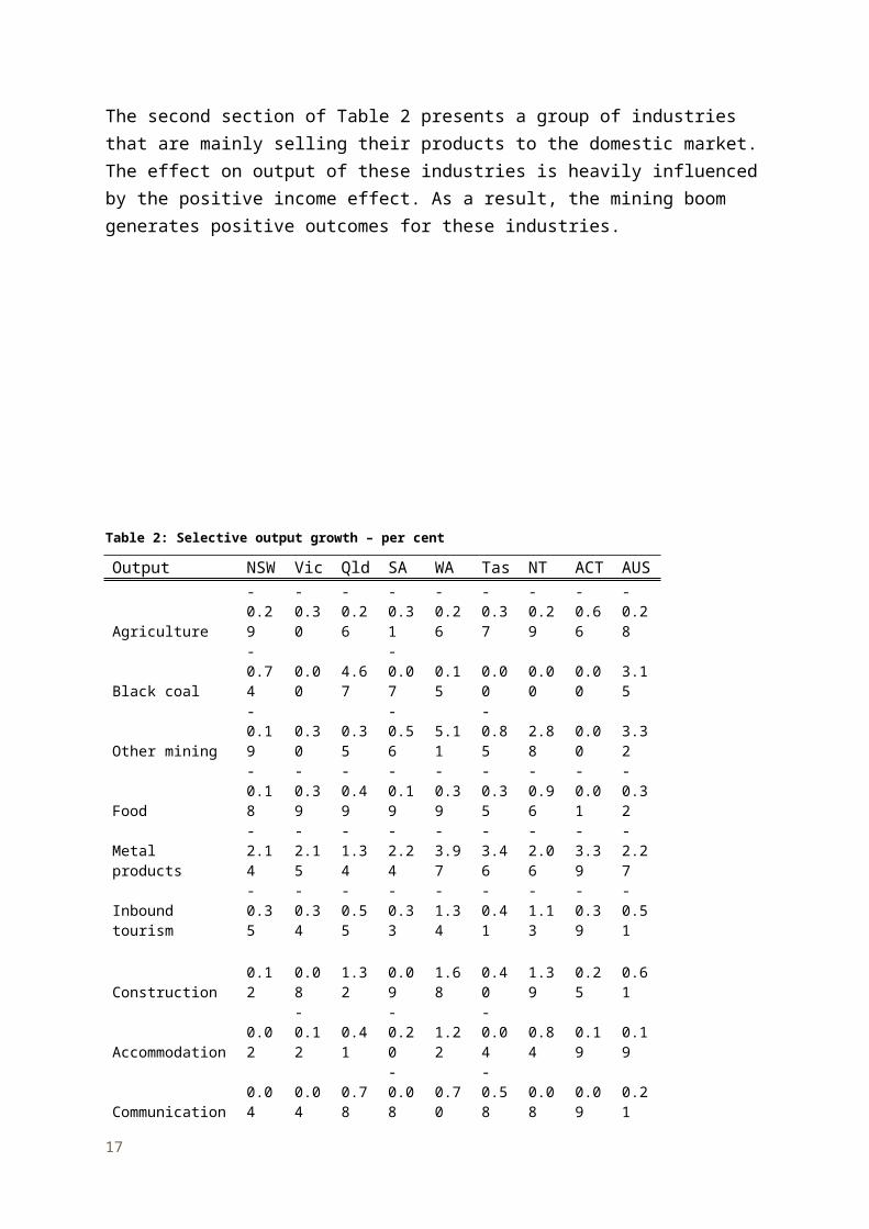
Table 5: FIFO impacts on demand for tourism – percentage point changes

Leisure tourism NSW Vic Qld SA WA Tas NT ACT AUS

1 Aggregate tourism demand 0.11 0.10 -0.11 0.12 -1.23 0.17 -0.92 0.29 -0.092 Inbound tourism demand 0.03 0.03 -0.11 0.02 -0.73 0.01 -0.62 0.03 -0.093 Domestic tourism demand 0.15 0.13 -0.11 0.14 -1.42 0.20 -1.13 0.38 -0.09

4 Intrastate tourism demand 0.04 0.04 -0.12 0.03 -1.07 -0.02 -0.63 -0.01 -0.13

5 Interstate tourism demand 0.36 0.34 -0.09 0.29 -2.31 0.37 -1.32 0.42 -0.036 Outbound tourism 0.05 0.04 -0.16 0.02 -1.23 -0.10 -0.84 -0.02 -0.14

Source: Authors’ estimates

Table 6: Effect on prices from increases in supply of accommodation and air transport – percentage point changes

Accommodation Air transport Inbound Intrastate Interstatepercentage point change

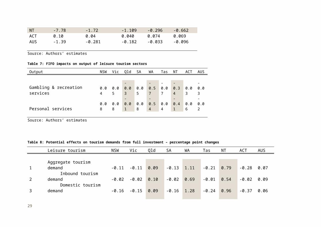
NSW 0.09 0.03 0.034 0.064 0.060Vic 0.09 0.04 0.036 0.059 0.047Qld -1.57 -0.45 -0.212 -0.043 -0.132SA 0.09 0.02 0.031 0.060 0.046WA -10.40 -1.97 -1.420 -0.547 -0.980Tas 0.11 -0.08 0.028 0.075 0.057NT -7.78 -1.72 -1.109 -0.296 -0.662ACT 0.10 0.04 0.040 0.074 0.069AUS -1.39 -0.281 -0.182 -0.033 -0.096

Source: Authors’ estimates

17

Table 7: FIFO impacts on output of leisure tourism sectors

Output NSW Vic Qld SA WA Tas NT ACT AUS

Gambling & recreation services 0.04 0.05 -0.03 0.05 -0.57 -0.07 -0.34 0.03 -0.03Personal services 0.08 0.08 -0.01 0.08 -0.54 0.04 -0.41 0.06 -0.02

Source: Authors’ estimates

Table 8: Potential effects on tourism demands from full investment – percentage point changes

Leisure tourism NSW Vic Qld SA WA Tas NT ACT AUS

1 Aggregate tourism demand -0.11 -0.11 0.09 -0.13 1.11 -0.21 0.79 -0.28 0.072 Inbound tourism demand -0.02 -0.02 0.10 -0.02 0.69 -0.01 0.54 -0.02 0.093 Domestic tourism demand -0.16 -0.15 0.09 -0.16 1.28 -0.24 0.96 -0.37 0.06

4 Intrastate tourism demand -0.07 -0.07 0.11 -0.07 0.94 -0.04 0.58 -0.03 0.095 Interstate tourism demand -0.34 -0.33 0.06 -0.29 2.12 -0.39 1.11 -0.41 0.006 Outbound tourism -0.09 -0.08 0.13 -0.07 1.04 0.01 0.75 -0.04 0.08

Source: Authors’ estimates

18

Table 8 presents the impacts on tourism demand from the case that accommodation and air transport sectors undertake full investment to increase their production capacity to respond to the high demand from FIFO. The results are in average annual percentage point change form.

As prices become more favourable in the mining boom states, demand for tourism in this scenario is marginally stronger than that in the base case for these three states. However, because the income effect is more dominant than the exchange rate effect in the mining boom regions, domestic tourism demand increases relatively more strongly than the increase in inbound tourism demand. As expected for the income effect, intra-state tourism demand increases in the three mining boom states more strongly than in the base case. Furthermore, interstate tourism demand is very responsive to price signals, particularly in Western Australia and Northern Territory. The effects in Queensland are relatively more modest than for the other two mining booms states because the price changes are not significant in Queensland.

In total, the aggregate demand of tourism is able to increase by 0.07 percentage points in annual average terms above the level in the base case when accommodation and air transport respond fully to FIFO demand.

An interesting point observed here is that in both the FIFO and investment cases, while intrastate tourism demand can result in a net gain or a net loss at the national level, interstate tourism demand appears to have a zero sum at the aggregate national level (Tables 5 and 8, row 5). As prices changes among states, interstate visitors move around states to take advantage of cheaper offers but the net change at the national level is zero.

Conclusions

The current mining boom has brought benefits to the Australian economy, but these benefits are not shared evenly across all states and territories. The most favourable condition of the boom remains in the mining boom states, while other states incur the costs of the crowding out effects. The two-speed economy is apparent through the net effects on GSP (row 1) presented in Table 1. The key effect from the mining boom is the increase in the price of exports, associated with an appreciation of the domestic currency. This drives the crowding out effect. Apart from the mining sectors, all other export-oriented industries are adversely affected by the currency appreciation. Industries that have a large proportion of their output serving the domestic market, on the other hand, benefit from the boom through the income effect.

The effects of the mining boom on the tourism sectors are mixed. The impact on the supply side is different from that of the demand side, depending on whether the consumption is for business or leisure tourism.

Given the dominant income effect and subsequent upward price effect generated by the mining boom, the boom stimulates domestic tourism demand positively while reducing

19

international inbound tourism demand across all states and territories. Of the domestic tourism demand, particularly in the mining boom states, interstate tourism suffers from the boom due to the price effect that the boom creates in the mining states. Interstate travellers shift away from Western Australia and Northern Territory as these two states become more expensive compared to all others. Queensland partly avoids the loss of interstate tourism demand as the price effect in the state is not as severe. The effect on outbound tourism is particularly pronounced in the presence of the strong appreciation in the domestic currency and the income effect. Overseas trips become substitutes for domestic trips when the exchange rate is in such a favourable condition.

FIFO is an expensive exercise for the mining sectors to adopt but the strong increase in mining exports due to higher commodity prices make it more profitable for the mining sectors to increase output without a real need to keep the cost down. Thus, in the first instance, FIFO generates a strong positive effect (benefit) on the accommodation and air transport sectors, as rapidly increasing demand leads to higher prices. The effect on price increases for these two sectors is significant as the simulation results indicate in Table 4. Between the two, accommodation prices increase much more strongly than air transport prices because all tourism categories use accommodation but not all of them (in particular intrastate tourism) use air transport. Among the mining states, price changes are much stronger in Western Australia and Northern Territory than those in Queensland. This is because usage of accommodation and air transport for FIFO is not as strong for black coal production in Queensland as it is for other mining in Western Australia and Northern Territory.

The results demonstrate that the strong business tourism demand from FIFO has severe impacts on demand for leisure tourism. This is a result of competition from FIFO for aviation services and accommodation driving up travel prices leading to travel becoming more expensive and the diversion of services available for leisure tourism to FIFO. At the aggregate level, leisure tourism demand declines (Table 5). Thus on the demand side, the mining boom affects the two groups (business and leisure travel) in opposite directions. The reduction in demand for leisure tourism in turn has negative impacts on the supply of other tourism services for leisure purposes such as gambling and recreation services, and personal services. Therefore, within the tourism supply side some sectors are growing while others decline, depending on their association with different types of tourism demand, business or leisure. This phenomenon is consistent with the obvious reality in the mining areas that tourism providers for leisure demand are struggling, while sub-sectors of tourism which provide services to business travel grow strongly. Even where business visitation is strong, it will often require different services from the visitors for leisure. Small business operators in the leisure tourism sector tend to be particularly adversely affected.

The negative impacts of FIFO on leisure tourism arise mainly because accommodation and air transport services do not respond quickly enough to rapid growth in FIFO related demand by expanding their capital stock. This is likely to be especially the case where uncertainty exists about the investment outlook and durability of the boom. In the scenario where these

20

two sectors do expand services in response to the increased demand for accommodation and air transport, the increase in supply alleviates price pressures on the market and generates a positive effect for the leisure tourism sector. The benefit is mainly distributed among the mining boom states and comes—to some extent—at the cost of tourism in non-mining boom states. The net effect, however, is an increase in tourism demand at the national level. From a tourism perspective, both leisure and business tourism benefit from investment occurring in aviation services and accommodation to meet FIFO generated demand. Such investment may also be of benefit to tourism sectors when the boom eases, to the extent that the investment provides infrastructure that will support future leisure tourism growth. The modelling results also suggest that investment to meet FIFO demand in these sectors generates net positive effects on the economy as a whole.

21

Appendix 1: The Tourism CGE Model

The Computable General Equilibrium (CGE) tourism model used in this project, MMRF-Tour, was developed on the base of the MMRF model of the Centre of Policy Studies at Monash University, Melbourne (Adams, 2008). A tourism module has been explicitly embedded into the core MMRF model, to incorporate detailed information on domestic tourism expenditure, and inbound tourism expenditure.

The conventional Input-Output (I-O) database of a CGE model does not present tourism expenditure data explicitly. In other words, final demand data in the CGE database includes both tourism and non-tourism data under the same final demand category. As a result, tourism impact analysis using the conventional CGE database is unable to capture the impact of tourism on non-tourism. Furthermore, it does not provide easy access to measure the tourism impact for scenarios such as an increase in total domestic tourism expenditure or decrease in total inbound tourism expenditure easily.

Given the importance of tourism in an economy, and the ability that a CGE model can offer for the impact analysis and the availability of TSA data, the tourism sector has been explicitly included in the database of MMRF-Tour as indicated in Figure 2. In the Tourism CGE database, two new industries Dtour and Etour have been created, for domestic tourism and inbound tourism respectively. The final household consumption is decomposed into tourism and non-tourism parts for each commodity, and the tourism part is moved to the intermediate quadrant to represent the domestic tourism supplier. Similarly, elements of Etour are extracted from the export vector. The tourism sectors Dtour and Etour do not require primary inputs. They act as a middle man to select all goods and services for tourism activity, and then sell all tourism services to the corresponding tourists (Pham, Simmons and Spurr 2010; Dwyer Forsyth, Spurr and Ho, 2003; and, Madden and Thapa, 2000). Dtour is not purchased by any users in the economy other than the household sector and, similarly, Etour by the export. These purchases of tourism services are defined as domestic and inbound tourists’ consumption respectively.

22

Figure 3: Database structure of the MMRF-Tour

IndustryJ1 J2 J3 … Jn Dtour Etour

Final DemandsHH INV GOV EXP

Value Added P1: Compensation of employees (COE)P2: Gross operating surplus & mixed incomeP3: Net taxes on products P4: Net taxes on productionP6: Imports

T2: Australian Production

T1: Total Intermediate use

Total Supply

C1

C2

Cn

Dtour

ETour

C11

C21....

Cn1

HH1NT

HH2NT....

HHnNT

Tot_Dtour

0

E1NT

E2NT....

EnNT

0

Tot_ETour

TS1

TS2....

TSn

Tot_Dtour

Tot_ETour

TC1 .. TC3 .....................TCn Tot_Dtour Tot_ETour C I G E

C22 ...............................C2n

COEGOSPTAXCTAXM

Total

0 00 0

0 0

(Not available)(Not available)

(Not available)

E1T

E2T....

EnT

0

0

HH1T

HH2T....

HHnT

0

0

Apart from the modification of the database, the theoretical structure of the CGE core remains unchanged. The model description is well documented in Adams (2008).

The MMRF model is a CGE model of all of the Australian state and territory economies with supply and demand explicitly captured7, and includes the following features:

households maximise utility by choosing the cheapest source for their purchases firms maximise profits by sourcing intermediate inputs from the cheapest source firms choose the right mix of labour, capital and land to reduce the cost of primary inputs

by a substitution among these primary inputs based on individual cost factorsstrong response by firms to large changes in input prices by undertaking technological innovation

domestic producers face a downward sloping export demand curve to reflect an assumption of a small open economy

investors are cautious in their investment decisions. For every subsequent increment in capital growth, investors require a higher rate of return to supply the same amount of additional investment

investors minimise their costs by choosing the cheapest source, as do producers, except that investment activity does not require primary inputs.

As seen in Figure 2, the tourism module focuses on the demand side, allowing analysis of the impacts on, or changes to, demand for tourism. Tourism activity is recognised by interstate,

7 This framework is referred to as a fully bottom-up model in the modelling terminology.

23

intrastate, inbound and outbound tourism. While expenditure of all other tourism sectors is spent entirely within the domestic economy, only a part of the expenditure of the outbound tourism sector is spent in the domestic economy with the majority spent outside Australia. The tourism CGE model explicitly captures only that proportion of outbound expenditure that is spent within Australia. The proportion spent outside the Australian economy is included in the original imports of goods and services by the household sector.

The interstate tourism sector is modelled to be driven by the income level of the origin (visitors') region (state) and relative tourism prices among destination regions (states). This means that higher income in one state will encourage visitors from that state to travel more. However, among the destination regions, the cheapest state will attract more visitors than other, relatively more expensive, destinations.

Inbound tourism is modelled to have a downward sloping demand curve as is the case for all other exports. Hence, the inbound tourism sector is adversely affected by increases in domestic production costs, just like all other conventional exports of domestically produced goods and services; and vice versa, the inbound sector is positively related to a lower cost of domestic production for better international competiveness.

The Tourism CGE model can be used in dynamic or comparative static mode. For simplicity, the MMRF tourism model was used in a comparative static mode for the mining boom project. Results can be interpreted as average impacts in a typical year during the timeframe of interest, two years for the short run, or six to seven years for the long run.

In modelling the mining boom, a long run closure was adopted to examine impacts on the economy, for example changes to GDP, GSP and all related components of the GDP/GSP in the expenditure side such as household consumption (C), investment (I), government consumption (G), exports (X) and imports (M). Policy makers are also keen to look at how this final outcome is achieved, particularly if there are winners and losers in the transitional period.

The following long run scenario assumptions were adopted:

Employment is fixed (at full employment). The real wage rate adjusts to settle the labour market.

The economy-wide rate of return is fixed. The capital stock changes to settle the capital market.

Household consumption is determined by income generated in the economy. Investment rates are indexed to capital growth. Consumption by state and federal governments is indexed to movements in GSP and

GDP respectively.

24

Appendix 2

Data in Table 9 show that although the other mining sector in Northern Territory is much smaller than those included in the table, the shares of accommodation and air transport services used by other mining in Northern Territory are much higher. This reinforces the fact that the mining sector in Northern Territory had used these services for FIFO much more than the mining sectors in all other states.

Table 9: Usage of accommodation and air transport services by mining sectors

Black coal in Qld Other mining - WA Other mining - NT$m % in total cost $m % in total cost $m % in total cost

Accommodation 22.56 0.14 66.6 0.26 19.34 0.40

Air transport 13.32 0.0849.29 0.19 13.50 0.28

Source: Adams, 2008

25

Appendix 3: FIFO impacts

Table 10: Impacts of FIFO on macro variables – percentage point change

NSW Vic Qld SA WA Tas NT ACT AUS1 GDP 0.052 0.052 -0.084 0.049 -0.868 -0.010 -0.608 0.052 -0.0972 HH 0.055 0.048 -0.093 0.046 -0.916 0.010 -0.690 0.033 -0.0803 INV 0.035 0.036 -0.048 0.036 -0.722 -0.069 -0.418 0.023 -0.0994 EXP 0.029 0.058 -0.167 -0.002 -0.575 -0.299 -0.750 0.082 -0.1625 GOV 0.047 0.048 0.065 0.050 -0.112 0.017 0.094 0.041 0.0356 IMP 0.051 0.044 0.020 0.035 -0.273 -0.021 -0.106 0.041 0.002

7 Unit cost of labour -0.154 -0.161 -0.199 -0.162 -0.549 -0.221 -0.314 -0.188 -0.2118 Unit cost of capital -0.073 -0.072 -0.067 -0.067 0.007 -0.046 0.000 -0.086 -0.0589 CPI 010 GDP deflator -0.113 -0.114 0.055 -0.110 0.520 -0.137 0.681 -0.147 0.006

11 Exchange rate -0.04612 Terms of trade 0.227

13 Capital usage 0.034 0.035 -0.047 0.034 -0.718 -0.073 -0.416 0.022 -0.1014 Aggregate employment 0.063 0.065 0.007 0.063 -0.388 0.025 -0.257 0.066 0Source: Authors’ estimates

26

Table 10 presents the impacts of FIFO-related demand. Within Queensland, Western Australia and Northern Territory, the mining boom draws resources away from other industries thus raising the domestic production costs across all industries in these states. For a given level of mining export demand from the three mining states, the presence of FIFO imposes a further increase in export prices, making the domestic currency appreciate further8 (row 11). Thus in these three states, there is a further loss of export demand (row 4) for all export-oriented industries other than mining on top of the loss attributable to the mining boom alone. With the loss of exports from all exporting industries, the mining boom states do not require as much labour as in the case without FIFO, particularly in Western Australia and Northern Territory (row 14). This lowers the wage rates in the mining boom states. With lower demand for labour from the mining boom regions, other states are able to retain more labour within their economies (row 14, non-mining regions), which then helps reduce the wage rates in those states as well. Overall, FIFO actually reduces wage rates across regions due to the additional loss of total exports.

For the mining boom states, the effect of the additional loss of export demand on income due to FIFO is much stronger than the effect of an improvement in the terms of trade. Household consumption in the mining states is thus reduced. The reduction in exports also leads to lower demand for capital (row 13). Thus investment is also reduced in the presence of FIFO (row 3).

For the non-mining boom states, the reduced wage rate boosts exports in those regions more than in the case with FIFO demand. Thus, coupled with the improvement in the terms of trade, more exports from these regions actually boosts household consumption (row 2), and induces more investment (row 3).

Overall, the total gain from the non-mining states is smaller than the losses from the mining states, which results in a net loss to GDP by 0.097 percentage points annually on average.

8 For simplicity, exchange rate is defined as the amount of domestic currency per unit of foreign currency. A decline (negative) in the exchange rate implies more foreign currency is required to obtain a unit of Australian currency. This would make Australian exports more expensive for foreign buyers.

27

Appendix 4: Potential impacts from full investment in accommodation and air transport

Table 11: Potential impacts of full investment – percentage point change

NSW Vic Qld SA WA Tas NT ACT AUS1 GSP/GDP -0.047 -0.048 0.041 -0.050 0.388 -0.035 0.241 -0.052 0.0272 Household consumption -0.075 -0.069 0.083 -0.070 0.782 -0.064 0.598 -0.061 0.0483 Investment -0.041 -0.042 0.051 -0.046 0.381 -0.016 0.235 -0.040 0.0424 Export -0.098 -0.114 0.054 -0.103 0.263 -0.092 0.426 -0.125 0.0225 Government consumption -0.047 -0.048 -0.071 -0.051 -0.053 -0.050 -0.244 -0.046 -0.0556 Import -0.048 -0.042 0.047 -0.042 0.396 -0.042 0.264 -0.048 0.026

7 Unit cost of labour 0.105 0.112 0.209 0.110 0.560 0.159 0.581 0.130 0.1838 GDP deflator 0.086 0.088 0.006 0.086 -0.201 0.116 -0.280 0.108 0.032

9 Real devaluation - - - - - - - - 0.01410 Terms of trade - - - - - - - - -0.038

11 Capital usage -0.04 -0.04 0.06 -0.04 0.40 -0.01 0.25 -0.04 0.0512 Aggregate employment -0.05 -0.05 0.01 -0.05 0.29 -0.05 0.12 -0.06 0

Source: Authors’ estimates

28

In the full investment response scenario, supply of accommodation and air transport in the three mining states is not constrained and increases in supply of these sectors alleviate the increases in their prices, reducing the cost of production to the mining sectors. Thus, for the same level of demand for mining exports as in the base case, the three regions now export their mining product at a lower price to foreign purchasers. This implies a weaker appreciation in the domestic currency compared to the base case (row 9)9.

Given a weaker appreciation in the real exchange rate, exporting industries other than the mining sectors in the mining boom regions are not as adversely affected as in the base case, thus exports from Queensland, Western Australia and Northern Territory are slightly higher than their levels in the base case (row 4). Consequently, those mining regions would require more resources to maintain the higher level of total exports; both labour and capital usage in this case are higher than the base case (rows 13 and 14).

Stronger production in mining boom states generates higher income levels. This leads to stronger household consumption in these states than those in the base case (row 2). Also, more capital demand in the mining states requires more investment than in the base case (row 3).

Stronger production in the mining states attracts more labour away from the non-mining boom states, resulting in wage rates slightly higher than those in the base case across all states. This makes exports from the non-mining boom states more expensive, hence losing export demand from these regions in overseas markets (row 4).

Overall, non-mining boom states have lower GSP in this scenario compared to the base case. However, the gain from the mining boom states over-offset such reductions to generate a net average annual increase in GDP of 0.027 percentage points.

9 A positive change in the exchange rate here implies less foreign currency is required to obtain the same unit of Australian currency, making Australian exports relatively cheaper.

29

References

Adams, P. (2008), MMRF: Monash Multi-Regional Forecasting Model - A Dynamic Multi-Regional Applied General Equilibrium Model of the Australian Economy, Centre of Policy Studies, Monash University.

Australian Bureau of Statistics (2012), Australian National Accounts: Input-Output Tables – Electronic Publication 2008–09, Cat. No. 5209.0.55.001

Australian Bureau of Statistics (2008), Australian National Accounts: Input-Output Tables – Electronic Publication 2004–05, Cat. No. 5209.0.55.001

Dwyer, L., Forsyth, P., Spurr, R., and Ho, T.V. (2003), “Contribution of tourism by origin market to a State economy: A multi-regional general equilibrium analysis”, Tourism Economics, 9(4), 431–448.

Madden, J.R., and Thapa, P.J. (2000), The contribution of tourism to the New South Wales economy: A multi-regional general equilibrium analysis, CREA Research Memorandum. Hobart, Tasmania: Centre for Regional Economic Analysis, University of Tasmania.

Pham, T. D., Bailey, G., and Marshall, J. (2013), The economic impacts of the current mining boom on the Australian Tourism Industry, Tourism Research Australia, Canberra, January 2013.

Pham, T. D., and Dwyer, L. (2013), Tourism Satellite Accounts and their applications in CGE Modelling, in Tisdell (eds), Handbook of Tourism Economics, chapter 22, World Scientific Publisher.

Pham, D. T., Simmons, G. D., and Spurr, R., (2010), “Climate change induced economic impacts of tourism destinations: the case of Australia”, Journal of Sustainable Tourism, Special Issue, Vol. 18, No. 3, April 2010.

30