Money and Elections What is the impact of Campaign Spending on Congressional Elections?

The Political Geography of Congressional Elections
Michael Crespin University of Georgia
David Darmofal University of South Carolina
Carrie Eaves University of Georgia
Paper prepared for presentation at the Annual Meeting of the Midwest Political Science Association, Chicago, IL, March 31st-April 3rd, 2011. We thank Jan Box-Steffensmeier, Greg Caldeira, Chuck Finocchiaro, William Minozzi, Ellen Moule, Craig Volden, Jeremy Wallace, and seminar participants at Ohio State University for helpful feedback, comments, and suggestions on this project. Of course, we thank Gary Jacobson for sharing his congressional elections data.

1
Introduction
The past decade has been marked by a renewed interest in political geography among
political scientists (Cho and Gimpel 2010, Darmofal 2009, Franzese and Hays 2007, Ward and
Gleditsch 2008). Although political geography had once played a prominent role in political
science research (e.g., in Key’s (1949) classic study of Southern politics), interest in geography
had waned in subsequent decades. The renewed interest in political geography has been
prompted by three simultaneous developments. There has been a marked increase in the number
of available geocoded datasets. At the same time, significant advances have been made in spatial
estimators and models, allowing scholars greater flexibility in modeling the spatial dimension of
their theories. Simultaneously, spatial estimation has been made more feasible by rapid advances
in computing technology. As a consequence, scholars interested in political geography can
increasingly examine how geography conditions the behaviors of interest to them.
Interestingly, despite the increased interest in political geography, studies of
congressional elections still largely ignore the geographic dimension of elections. Most studies
of congressional elections treat them as independent contests. Links across elections are largely
assumed to be limited to elections exhibiting partisan tides, and even here the geographic
component is typically subsumed to expectations of a national wave. Indeed, to the extent that
geography is incorporated in studies of congressional elections, the modal way in which it is
incorporated is via a dummy variable that allows the intercept to vary between contests in the
South and the non-South.
We believe this approach is problematic. Congressional elections are not independent
contests. Even though they occur in geographically distinct locales, spatially proximate contests
are linked through a variety of mechanisms. Party labels mean different things – and carry

2
varying degrees of importance – across congressional elections. Party organizations similarly
vary spatially in their organizational strength and resources and in their effects on congressional
elections. Campaign expenditures are not equal in importance across U.S. House races, but
instead vary in the benefits they can bring for candidates depending upon the cost of media
advertising and the geographic expansiveness of districts. Media markets themselves are not
wholly contained within congressional districts but instead span neighboring districts. We
expect, in short, that factors shaping congressional elections vary spatially, with their effects
more similar the more spatially proximate the congressional districts are.
Our expectation of spatial heterogeneity in parameters differs considerably from the
current, one-size-fits-all approach to the study of congressional elections. We examine this
heterogeneity via Geographically Weighted Regression (GWR) models, which allow behavioral
parameters to vary spatially rather than assuming that these parameters are constant across the
spatial plane. We employ GWR models to standard congressional election models of incumbent
vote share for each congressional election from 1992 through 2006. We find evidence of
extensive spatial heterogeneity in the effects of standard predictors of incumbent vote share such
as the normal vote, total campaign spending, the presence of a quality challenger, the freshman
status of the incumbent, and the incumbent’s party. Moreover, the GWR models explain a
greater proportion of the variance than standard OLS models in each congressional election and
demonstrate a superior model fit over standard OLS models in all congressional elections but
one.
Below, we first review some of the previous research on elections and argue why it is
especially important to think about spatial heterogeneity in the context of congressional
elections. Second, we outline our method, geographic weighted regression and explain how it

3
can help to answer questions regarding spatially varying regression coefficients. Third, we
present our data and results for elections from 1992-2006 and finally conclude with a discussion
of why political geography can influence election results.
Elections and Political Geography
In the vast literature on congressional elections, certain features have been shown to
consistently influence outcomes including the presence of a quality or experienced challenger
(Jacobson and Kernell 1983, Jacobson 1989), the seniority of the incumbent (Alford and Hibbing
1981) underlying levels of districts partisanship measured independently of the candidate’s vote,
and of course, spending (Jacobson 1978, 1980).
To date, researchers have assumed that these factors affect outcomes in a similar fashion
in all parts of the country and are not influenced by varying "politics on the ground" above and
beyond the standard measures associated with congressional elections. We think this notion
might be tenuous at best since elections are frequently discussed and contested in the context of
political geography. For example, we often use phrases such as the "solid South," (Herbert 1890,
Frederickson 2000) to portray the one-party dominance in the South or refer to some elections as
taking place in "swing" or "battleground states" (Lamis 2009). This type of language implies that
elections in some places are different than others. Of course, our idea is not new since Key
(1949) theorized about how "friends and neighbors" and localism and sectionalism can drive
election outcomes well before election reporters highlighted results on their red and blue maps.
When geography does receive some theoretical attention from scholars, that
consideration is frequently limited to general controls for region. For example, in order to control
for the unique nature of the South in electoral politics many scholars would simply include a

4
dichotomous variable that represented the thirteen states of the former confederacy (e.g. Glazer
and Robbins 1985, Cox and Munger 1989, Branton 2009). Controlling for the South in this
fashion makes the implicit assumption that the features that make a state “southern” are similar
across each of the states. This may be unreasonable given the rich sub-field dedicated to southern
politics (e.g. Key 1949, Black and Black 2002, Bullock and Rozell 20010)
While the South may have some distinctive features, these controls treat the other thirty-
seven states the same, despite the fact that the political nature of states such as South Dakota and
Massachusetts varies greatly. Other works control for various regions of the country including
dichotomous variables for East, South, Midwest, West and North (Johannes 1983). Yet even
these regional controls treat all districts within one region similarly when we know that districts
vary greatly and can be influenced by the political context of neighboring congressional districts.
One area where geography plays a featured role is redistricting since it explicitly deals
with drawing and redrawing political boundaries (e.g. Bullock 1975, Abramowitz 1983, Butler
and Cain 1992, Gelman and King 1994, Canon 1999, Epstein and O'Halloran 1999,
Ansolabehere, Snyder and Stewart 2000, Cox and Katz 2002, Heatherington, Larson, and
Globetti 2003, Brunell 2008, Crespin 2010). Although this literature is theoretically rich, it does
not always adequately address geography methodologically. First, we should question the
assumption that election results are independent across neighboring districts. If districts were
drawn randomly, then this assumption should be safe. Yet, we know this is not the case since
districts are drawn with politics -- specifically winning elections -- in mind (Born 1985). In
practice some members are safer after a redistricting because co-partisans were drawn into their
district while others are made worse off when favorable areas were cut out of their districts.
Since districts share boundaries, it is not possible to change one district without altering another.

5
At the very least, this suggests examining the residuals of regressions to look for spatial
autocorrelation.
In addition to questions related to independence, studying election results with an eye
towards political geography may help us think about some of the puzzling results from the
redistricting literature. For example, Erickson (1972) and others (Tufte 1973, Mayhew 1974,
McKee 2008) suggested that redistricting can increase the incumbency advantage while some
(Cover 1977, Ferejohn 1977, Abramowitz, Alexander, and Gunning 2006) have not found any
support for this hypothesis. It is possible that the incumbency advantage is increased in some
areas while lowered in others. The approach we outline below will allow us to look for regional
results along these lines.
Although political geography is rarely explicitly incorporated into models of
congressional elections, there are other strong reasons for including geographic influences on
elections in our models. Indeed, one of the defining features of the United States is its
geopolitical diversity (Gimpel and Schuknecht 2003, Chinni and Gimpel 2010). In a nation as
diverse as the United States, one in which localism and sectionalism have played critical roles in
its development, we should not expect political, social, or demographic factors to play the same
roles in shaping elections across the United States. Instead, these factors are likely to vary
geographically in their effects, producing geographic variation in elections.
There is, in fact, reason to believe that geography plays a critical role in conditioning
elections based upon the limited number of studies that have taken political geography seriously.
One of the seminal literatures on elections, the realignment literature, has emphasized a critical
role for political geography in elections. Dating back to Key’s (1955, 1959) analyses of critical
and secular realignments, there was the recognition that realignments are not large, national

6
events that were experienced similarly in all locales. Instead, realignments, in this view, are
geographically located events, producing enduring shifts in the aggregate partisan balance in
some locations but not in others as a consequence of the differential impact of the realigning
issues across the country. More recently, Nardulli (1995, 2005) has examined and documented
the influence of political geography in realignments while Darmofal (2008) demonstrates that
covariates varied in their effects on elections during the New Deal realignment.
The realignment literature highlights the fact that elections are geographically located and
that contests in neighboring locales may share similarities due to their geographic location.
Another literature that examines the geographic connections between elections focuses on the
critical role of fundraising networks in election campaigns. Cho (2003) documents the spatial
structure of campaign donations by Asian Americans. Gimpel, Lee, and Pearson-Merkowitz
(2008) document the partisan and strategic motivations that lead out of district campaign donors
to contribute to congressional campaigns. More recently, Cho and Gimpel (2010) have
demonstrated the geographic patterning of contributions and volunteering in a Texas
gubernatorial campaign. Important for our analysis, this last study also demonstrates the
extensive spatial nonstationarity in the factors that influence contributions and volunteerism in
political campaigns.
Interestingly, while there has been only limited analysis of political geography’s
influences on elections in the United States, comparative elections scholars have been keenly
interested in the role of geography during elections in other countries. O’Loughlin, Flint, and
Anselin (1994) demonstrate the strong geographic patterning in electoral support for the Nazi
Party in the election of 1930. Fernandez-Duran, Poire, and Rojas-Nandayapa (2004) examine the
role of spatial effects in direct elections in Mexico. Johnston and co-authors have examined

7
geographic effects in elections in the United Kingdom in a series of articles (see, e.g., Jones,
Johnston, and Pattie 1992, Pattie, Johnston, and Fieldhouse 1995, Johnston et al. 2005).
In short, studies of the influence of political geography on elections in the United States,
and of congressional elections in particular, have been quite limited. This lack of a geographic
component to our models of congressional elections is, however, quite problematic. As the early
realignment literature in the U.S. demonstrated, and the emerging spatial literature on campaign
donors has confirmed, geography plays a critical role in U.S. elections. Our understanding of
congressional elections would benefit from incorporating the geographic orientation of many
comparative elections scholars.
Political Geography in Congressional Elections
Above, we discussed several general reasons why we should think about elections in the
context of political geography. In this section, we will be more explicit about why we expect a
set of covariates that can explain congressional elections to exhibit spatial heterogeneity.
Normal Vote
Many studies of congressional election outcomes assume that the normal vote, or
underlying political conditions, has a strong influence on electoral margins (e.g. Carson and
Engstrom 2005, Carson, Engstrom, and Roberts 2007). The logic is quite simple with the
expectation that when the normal vote is in the candidate's favor, they should receive more votes,
all else equal. However, we think it is possible to find significant variation in the strength of this
relationship across the country for a few reasons. First, as the realignment literature tells us, the
attachment voters have to political parties is not the same everywhere. If an area is going through
a secular realignment then underlying political conditions may not carry as much weight in any

8
particular congressional election compared to areas where the attachment to party identification
is stronger. This goes hand in hand with the notion that campaigns in some areas are party driven
affairs while others are more candidate centered. Based on these factors, we expect to find some
variation in the ability of the normal vote to predict congressional election outcomes.
Congressional Spending
Although there are debates surrounding just how spending can influence election
outcomes, in seems reasonable to expect that increased total spending should lead to more
competition. 1 However, because the cost to running a campaign is not constant across the
country, it seems reasonable to expect to find varying returns to spending on election outcomes.
Research on political advertising has made clear that the costs to buying a television
advertisement can differ so a dollar spent in one race may not buy the same amount of coverage
as other districts. In addition, some districts are well contained within media markets while
others split markets. If a candidate needs to buy ads in multiple markets, they will have to spend
more to reach the same set of voters. On top of the costs to purchasing ads, running campaigns
may cost more in some places due to the high price of renting office space or other campaign
related needs. Finally, candidates seeking to represent districts that are large geographically will
have to spend more in order to campaign in all areas of the district. So, for several reasons, we
should not expect spending to increase competition at the same rate everywhere.
Quality Challengers
Jacobson and Kernell (1983) and Jacobson (1989) have demonstrated that quality or
experienced candidates typically earn a higher percentage of the vote compared to political
1 Jacobson (1978) finds that challenger spending is effective in increasing name recognition and a challenger’s chances of winning, while incumbent spending is ineffective at influencing election outcomes. For an alternative view see Green and Krasno (1988) who find that incumbent spending is influential.

9
amateurs. In general, there is strong support for their hypotheses. Yet, the standard dichotomous
measure for quality challenger is rather blunt and treats all experience as equal so it seems
reasonable to expect that experienced challengers from some regions will be better candidates
compared to others. For example, many quality challengers get their early campaign experience
from running for the state legislature and these can vary in their degree of professionalism
(Squire 2007). This in turn can surely affect a challenger's ability to run a campaign (Berkman
and Eisenstein 1999) since more professional state legislators should be better equipped to take
on congressional incumbents. In addition, other work has demonstrated that the constituency
congruency between state legislative districts and congressional districts varies by state and
district and this can also influence election outcomes for quality challengers (Carson et al. n.d.).
Based on these factors, it is reasonable to expect to find some spatial heterogeneity for this
variable.
Party of Incumbent
One concept that can predict congressional election outcomes is the partisan affiliation of
the incumbent. In many election years, one party significantly outperforms the other. However,
this trend is rarely constant across the country since both parties tend to have their strong and
weak areas with Republicans generally running well in the South and Democrats doing better in
the Northeast and California coast. These trends tend to be more variable though throughout the
Midwest and Western states. In essence, we expect to find significant variation in this variable
since regional tides are rarely constant in all elections. In sum, there are many reasons to expect
geographic variability in congressional elections. Below we discuss the data and methods we will
use to look for these outcomes in congressional elections.
10
Data
Our dependent variable is the incumbent's share of the two-party vote for elections held
in 1992-2006.2 Since GWR is not well equipped to handle panel data, we look at each election
separately. In addition, we drop Alaska and Hawaii from our analysis since they are far from
other states and we would have to stretch the definition of "neighbor" for our analysis.
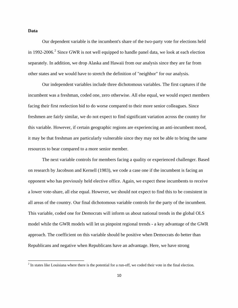
Our independent variables include three dichotomous variables. The first captures if the
incumbent was a freshman, coded one, zero otherwise. All else equal, we would expect members
facing their first reelection bid to do worse compared to their more senior colleagues. Since
freshmen are fairly similar, we do not expect to find significant variation across the country for
this variable. However, if certain geographic regions are experiencing an anti-incumbent mood,
it may be that freshman are particularly vulnerable since they may not be able to bring the same
resources to bear compared to a more senior member.
The next variable controls for members facing a quality or experienced challenger. Based
on research by Jacobson and Kernell (1983), we code a case one if the incumbent is facing an
opponent who has previously held elective office. Again, we expect these incumbents to receive
a lower vote-share, all else equal. However, we should not expect to find this to be consistent in
all areas of the country. Our final dichotomous variable controls for the party of the incumbent.
This variable, coded one for Democrats will inform us about national trends in the global OLS
model while the GWR models will let us pinpoint regional trends - a key advantage of the GWR
approach. The coefficient on this variable should be positive when Democrats do better than
Republicans and negative when Republicans have an advantage. Here, we have strong
2 In states like Louisiana where there is the potential for a run-off, we coded their vote in the final election.

11
expectations and presume that Democrats should do poorly in the South as this area has trended
towards the Republican Party over time. We might also expect to find Democrats doing well in
the Northeast, especially in more recent elections.
In addition to the dichotomous variables, we control for the underlying partisan strength
in the district measured with the incumbent's share of the presidential vote in the most previous
election. We expect this variable to be positive and significant since incumbents should do better
when partisan forces in the district are aligned in their favor. When we examine the influence of
this variable over space, it allows us to determine if incumbents are running ahead, or behind, of
the "normal" vote. The variation is likely driven by the attachment voters have to their member
of congress versus the party in general. If the coefficient is greater than average, then it is likely
the representative from that district has something akin to a strong incumbency advantage above
and beyond any partisan advantage. If the effect is small in comparison, then the incumbent is
running behind the normal vote.
Finally, we control for the total amount of spending in a district divided by $10,000. All
else equal, we should expect more money should lead to more competition (Jacobson 2009).
However, since the cost of running a campaign can vary across the country, we should not expect
the same returns to spending everywhere. For example, it may be prohibitively expensive to rent
office space in some urban districts and buying ads can also vary by media market (Ridout et al.
2002). While some research has controlled for the relative cost of advertising (Stratmann 2009)
most research assumes that the return to spending is constant in each congressional district.
Again, we argue that this is a tenuous assumption worth exploring. If we are correct, then there
should be significant variation in the coefficients. If we are wrong, then the coefficients should
be relatively equal everywhere. Given that our dependent variable, incumbent vote-share is

12
continuous, our initial set of results is from an OLS regression while the next set are from a
series of geographic weighted regressions.
Geographically Weighted Regression
There are a variety of modeling strategies for spatial heterogeneity. Scholars can adapt
the random coefficients model and estimate a spatial random coefficients model in which spatial
dependence in parameter variation around the mean is modeled (Anselin and Cho 2002).
Alternatively, in some applications researchers may feel confident in assuming that parameters
are homogeneous within discrete spatial subsets of the data but vary across these subsets. If so,
spatial switching regressions, also known as spatial regimes models, may be employed (see, e.g.,
Anselin 1990). Researchers may assume a constant drift in parameter values and model this
continuous spatial heterogeneity via spatial expansion models (see, Casetti 1972).
In this analysis, we employ Geographically Weighted Regressions (GWR) to model
spatial heterogeneity in parameters. This approach shares some similarities with the spatial
expansion modeling approach, but unlike that approach does not nest parameters as functions of
higher level parameters. Instead, GWR models allow for continuous spatial heterogeneity in
parameters by allowing more spatially proximate observations to exert a stronger influence on
location i’s parameter estimates than more spatially distant locations. To date, Geographically
Weighted Regressions have seen only limited application within political science. Among the
applications in political science are Calvo and Escolar (2003), Darmofal (2008), and Cho and
Gimpel (2010).

In the standard regression model, the effects of covariates are estimated as global
parameters that are not allowed to vary by unit.3 This produces the standard regression model
with non-varying parameters:
13
iy xi k k ik= + +β β ε0 Σ , (1)
in which yi is the ith observation on the dependent variable, β0 is the global intercept, xik is the ith
observation on the kth independent variable, βk is the parameter corresponding to the kth
independent variable, and βi is the error term for the ith observation. Geographically Weighted
Regressions depart from this standard regression framework by allowing the estimated
parameters to vary spatially. This produces a continuous spatial plane of parameter values, with
these parameters measured at particular observed locations, typically the centroids of the
observed units (Fotheringham, Charlton, and Brunsdon 1998, 1907). (In this paper's analysis, the
parameters are measured at the centroid of each congressional district in which we have observed
data). This produces the following model with spatially varying parameters:
y u v u v xi i i k k i i ik= i+ +β β ε0 ( , ) ( , ) ,Σ (2)
where, as Fotheringham, Brunsdon, and Charlton (2002, 52) note, “ui,vi denotes the coordinates
of the ith point in space and βk(ui,vi) is a realization of the continuous function βk(u,v) at point i.”
In calibrating equation (2), locations near i are given greater weight in influencing
βk(ui,vi) through a spatial weights matrix. We employ a bisquare weighting function that takes the
form:
3 The notation and presentation in this section follows Fotheringham, Brunsdon, and Charlton (2002, 52-64), and Fotheringham, Charlton, and Brunsdon (1998).

22
1⎥⎥⎦
⎤
⎢⎢⎣
⎡⎟⎟⎠
⎞⎜⎜⎝
⎛−=
bd
w ijij (3)
where dij is the distance between points i and j and b is the bandwidth, such that when
(Charlton and Fotheringham 2009, 7). The bandwidth reflects the distance-decay of the
weighting function and affects the spatial smoothing of the estimates, with smaller bandwidths
producing less spatial smoothing than larger bandwidths (Fotheringham, Brunsdon, and Charlton
2002, 45). A critical question, therefore, in any GWR analysis is the choice of the proper
bandwidth. In this analysis, we employ the bandwidth that minimizes the small sample corrected
form of the Akaike Information Criterion (the AICc). As Charlton and Fotheringham (n.d., 7)
note, this bandwidth estimation approach has the advantage over an alternative, commonly used
cross-validation approach in that it incorporates the complexity of the model into the bandwidth
choice.
0=ijw
bdij >
The GWR modeling approach we employ in this paper offers several advantages for our
analysis of spatial heterogeneity. First, rather than a priori defining breakpoints in parameters, as
would be the case with a spatial switching regressions approach, we allow the breakpoints to
emerge from the data as a function of the AICc values. Second, related to this concern, we’re
able to model spatial heterogeneity with much greater verisimilitude than would be the case with
an alternative approach such as the spatial switching regressions approach or a multi-level
approach which, at most, would model a few distinct regimes. Third, we do not impose the
assumption of spatial independence across regimes or strata that is inherent in these alternative
approaches for modeling heterogeneity. It is unrealistic, in our view, to assume that
congressional district from neighboring states, for example, are spatially independent of each
14

15
other as would be the case if states were used to define regimes or strata in the switching
regressions or multi-level modeling approaches (see also Darmofal 2009 on this point).
Results
Table 1 presents the results from eight separate OLS regressions, one for each
congressional election from 1992-2006.4 Since we are using these results as a baseline to
compare with results that account for spatial heterogeneity, we will only discuss them briefly.
First, we find that freshman members performed significantly worse than more senior
incumbents in just two elections, 1994 and 1996. In these elections, freshman received 2.5 and 4
percentage points less than incumbents who already survived their first reelection campaign.
Next, in all but one election, 2004, incumbents who faced quality challengers fared worse than
members who did not face an experienced opponent. For most elections, the substantive effect
was around 5 percentage points with the exception of 1998 where the effect was quite large, over
10 percent. The final dichotomous variable that controls for the partisan affiliation of the
incumbent performed as expected in 1994, 2006, and 2008 with the sign corresponding to
sizeable seat gains by the Republican (1994) and then Democratic Parties (2006 and 2008). The
variable was also negative and significant in 1996 and 1998 indicating Republicans did better, on
average, compared to Democrats, despite small seat gains for the minority Democratic Party.
The variable measuring underlying political conditions, presidential vote, was positive
and significant across each of the eight elections. The average coefficient size was 0.51, meaning
that for every one percentage point increase in presidential vote-share, the incumbent would see
an increase of just over one-half of a percentage of their congressional vote. Finally, the
4 We will include the 2008 and 2010 elections in future iterations of this paper.

16
spending variable was negative and significant for each election. Substantively, we can say that
on average, an incumbent's vote-share will decline by 5.9 percentage points if total spending in a
race reaches $1 million.
In addition to the coefficients and standard errors, we also repost the z-score for the
Moran's I statistic that measures global spatial autocorrelation in the residuals. If there is a
positive spatial relationship in the residuals, meaning positive (negative) errors are near other
positive (negative) errors then the z-score will be positive and significant. Our results indicate
there is statistically significant spatial autocorrelation in each of the eight regressions.5 Since we
are primarily interested in the spatial heterogeneity in the regression coefficients, we now turn to
diagnostics and results from the geographic weighted regressions.
Spatial Varying Coefficients
Before we present the coefficients from the GWRs, we report some simple diagnostics
that compare the two types of models in Table 2. In order to compare model fit, we first look at
the changes in the corrected Akaike Information Criterion (AICc) and then adjusted R2’s. In
terms of AICcs, the values are lower for the GWR models with the exception of the 1992 case.
The adjusted R2’s also show modest improvements across the board.6 We also find that only
three of the GWR models suffer from statistically significant (p < .05) spatial autocorrelation in
the residuals compared to all of the OLS models. In sum, these diagnostics suggest it is at least
worth exploring results from the GWR models.
5 We measure spatial autocorrelation using row standardized spatial weights matrices. If we only concerned with spatial autocorrelation in the residuals and not spatial heterogeneity in the coefficients, diagnostics indicate we could reduce the spatial autocorrelation with a spatial error model. 6 Of course, we need to be careful in declaring one model "better" than another since we do not know the true data generating process.

17
In Figure 1, we offer a comparison between the OLS coefficients and the range of
coefficients for the GWR models in each election year, 1992-2006. In each case, the red triangle
represents the OLS coefficient while the gray hash-marks denote GWR coefficients. If the
coefficient(s) in either model was not significant at the .05 level, we did not include it in the
figure. Not surprisingly, with a few exceptions, the OLS coefficients tend to fall within the range
of the GWR coefficients. However, there are some notable differences. For example, in 2002 and
2006, freshman actually performed better than more senior members according to the GWR, but
there was no significant difference in the OLS models. These results contrast from the previous
findings, and most of the literature, where members in their first reelection campaign do worse
than others. We also find that in 2000, the coefficient on the dichotomous Democrat variable is
positive and significant in some districts and negative and significant in others. A result like this
would not appear in a standard OLS model since the average effect is not distinguishable from
zero.
These results also demonstrate the considerable range present in GWR coefficients. For
example, in 1998, the coefficient on Quality Challenger ranges from -18 to -6 — a difference of
12 percentage points. The variation on spending is also pronounced in 1994. In some areas of the
country, an addition million dollars resulted in a decrease of the incumbent's vote-share by 10
percentage points while it was over 20 in others. Finally, the coefficient on the incumbent's share
of the presidential vote demonstrated extensive variation. For some elections, the range from
minimum to maximum was at least double. If we want to think of the OLS coefficient as the
average, substantively this means that some members are running well ahead of the normal vote,
possibly indicating an incumbency advantage, while others are running behind. Put another way,
if we predicted the vote for a Democrat in 2000 holding other variables and coefficients at their
18
means while letting the coefficient on this variable vary on its range, a member on the low end
where the coefficient is about .3 would expect to earn 64 percent of the vote while a member at
the high end, near .6 would be closer to 82 percent.7 This indicates that the considerable
variation in the size of the coefficients translates into meaningful substantive effects.
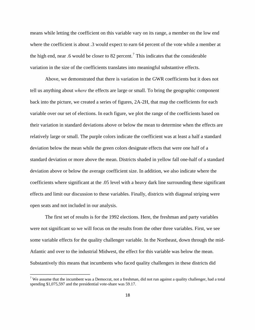
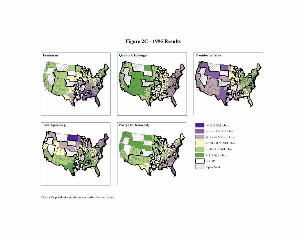
Above, we demonstrated that there is variation in the GWR coefficients but it does not
tell us anything about where the effects are large or small. To bring the geographic component
back into the picture, we created a series of figures, 2A-2H, that map the coefficients for each
variable over our set of elections. In each figure, we plot the range of the coefficients based on
their variation in standard deviations above or below the mean to determine when the effects are
relatively large or small. The purple colors indicate the coefficient was at least a half a standard
deviation below the mean while the green colors designate effects that were one half of a
standard deviation or more above the mean. Districts shaded in yellow fall one-half of a standard
deviation above or below the average coefficient size. In addition, we also indicate where the
coefficients where significant at the .05 level with a heavy dark line surrounding these significant
effects and limit our discussion to these variables. Finally, districts with diagonal striping were
open seats and not included in our analysis.
The first set of results is for the 1992 elections. Here, the freshman and party variables
were not significant so we will focus on the results from the other three variables. First, we see
some variable effects for the quality challenger variable. In the Northeast, down through the mid-
Atlantic and over to the industrial Midwest, the effect for this variable was below the mean.
Substantively this means that incumbents who faced quality challengers in these districts did
7 We assume that the incumbent was a Democrat, not a freshman, did not run against a quality challenger, had a total spending $1,075,597 and the presidential vote-share was 59.17.

19
worse compared to similar members in states such as South Dakota, Nebraska and parts of
Kansas, Oklahoma, Texas, and Louisiana. Since the districts further west are not inside the heavy
black lines, they are not statistically significant. In terms of the presidential vote, we see a
similar, but not identical regional breakdown. Here, incumbents in east coast states and parts of
Ohio and Kentucky are running well ahead of the normal vote while the effect is below the mean
for states west of Illinois and Mississippi. Finally, the spending variable is large in the Northeast
and the upper Midwest. This means more spending brings more competition in these regions.
This result contrasts with the coefficients from states around Texas where the returns to spending
were less. Based on just these results, it is readably visible that simply including regional control
variables may not capture all of the variation present in the regression coefficients.
Table 2B displays the results for 1994, where the Republicans regained control of the
House for the first time since 1954. In this election, there are some consistent strong effects in
Southern districts for several of the variables. First, members elected in 1992 did poorly in this
region, along with some areas in the Mid-Atlantic. More spending also bought greater levels of
competition in the South compared to the Northeast and a few districts in the heartland.
Consistent with the secular realignment in the late eighties and early nineties, Democrats fared
poorly in the South and the Mid-Atlantic. However the results also show they performed below
average further north through parts of the upper Midwest. In contrast, Democratic incumbents
did above average in New England and several of the western states.
In the next election where the Democrats picked up a net of eight seats, some of the
results are similar to previous elections while others differ. For example, freshman and
Democrats continue to do poorly in the South and Mid-Atlantic. However, in this election, the
returns to increased spending were low in the South and high in the Northeast. This stands in

20
contrast to the previous election where the results were largely reversed although the coefficient
range is not large this time around. In terms of the normal vote, Northeastern and Mid-Atlantic
incumbents were running ahead of the mean while incumbents in the West ran behind the
presidential vote in their district.
The 1998 elections represented the rare event where the out-party failed to pick up seats
in a midterm election. Compared to other elections, this is the year with the most variation in the
quality challenger variable. Along the most of the South and border states, the size of this
coefficient was large, translating to a decrease in over 16 percentage points in some districts. As
we head away from this region, the size of the coefficient dissipates down to just 6 points, closer
to the traditional average. Similar to 1992 and 1994, the returns to spending were larger in the
South, although effects were more isolated. In this election, the coefficients on the presidential
vote variable represent a bit of an anomaly since they are large in the West but smaller through
other parts of the country and near the average in the Northeast. Finally, Democrats did
significantly worse in parts of the deep South and Florida along with most of the Midwestern
districts.
Similar to 1994, the results in 2000 show some strong Southern effects, but this time they
continue out towards parts of the Southwest for a few variables. Incumbents who ran against
quality challengers lost between eight and 10 percentage points in this region compared to only
around five or less in districts further north. The returns to the presidential vote were weaker
here, while spending more led to increased competition. In terms of the party variable,
Democrats did well below average in Florida and a few other deep South districts where the size
of the coefficient was just under -4. This stands in stark contrast to New Mexico and parts of
west Texas, Oklahoma and Kansas where the coefficient was of similar magnitude, but in the

21
positive direction. The results on this variable demonstrate one of the key advantages to the
GWR approach as it allows for the coefficient to be positive in some places and negative in
others.
In the midterm election of George W. Bush's first term (Table 2F), the freshman variable
is actually positive and significant in Florida and parts of a few Southern states. This result is
likely driven by a few freshmen doing well in Florida and South Carolina. Again, this is a result
that we would not find using OLS since the freshman coefficient in the standard model was not
statistically significant. The other two variables with significant coefficients are somewhat
similar to past with more spending leading to increased competition in Texas and emanating
towards the North and West. Meanwhile, the results for the spending variable were below
average in the Northeast and Midwest. Once again, the coefficient on the presidential vote
variable was high in the Northeast and lower out west. This time, the effects were also low in the
South and high in the central Midwest.
In 2004, the last year before the Democrats returned to power, the out-party began to
make some inroads in the middle of the country as indicated by the above average coefficients in
the Midwest down through the old Southwest. Once again, the coefficient on the normal vote
variable was high in the Northeast, but this time the above average effects reach all the way
down the east coast. The below average effects in Western states match up well with many of the
previous elections.
In the final election in our dataset, 2006, the Democrats regained the House with a net
gain of 31 seats. Working our way through our by now familiar variables, the coefficient on
freshman was once again positive and significant, but this time in the western part of the country.
The effects for quality challengers were large in the deep South and in some of the border states.
22
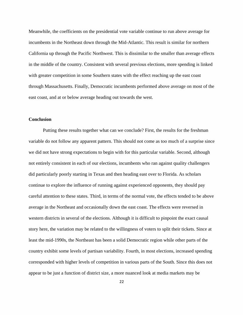
Meanwhile, the coefficients on the presidential vote variable continue to run above average for
incumbents in the Northeast down through the Mid-Atlantic. This result is similar for northern
California up through the Pacific Northwest. This is dissimilar to the smaller than average effects
in the middle of the country. Consistent with several previous elections, more spending is linked
with greater competition in some Southern states with the effect reaching up the east coast
through Massachusetts. Finally, Democratic incumbents performed above average on most of the
east coast, and at or below average heading out towards the west.
Conclusion
Putting these results together what can we conclude? First, the results for the freshman
variable do not follow any apparent pattern. This should not come as too much of a surprise since
we did not have strong expectations to begin with for this particular variable. Second, although
not entirely consistent in each of our elections, incumbents who ran against quality challengers
did particularly poorly starting in Texas and then heading east over to Florida. As scholars
continue to explore the influence of running against experienced opponents, they should pay
careful attention to these states. Third, in terms of the normal vote, the effects tended to be above
average in the Northeast and occasionally down the east coast. The effects were reversed in
western districts in several of the elections. Although it is difficult to pinpoint the exact causal
story here, the variation may be related to the willingness of voters to split their tickets. Since at
least the mid-1990s, the Northeast has been a solid Democratic region while other parts of the
country exhibit some levels of partisan variability. Fourth, in most elections, increased spending
corresponded with higher levels of competition in various parts of the South. Since this does not
appear to be just a function of district size, a more nuanced look at media markets may be

23
appropriate. Finally, the variation on the Democrat coefficient performed as expected with large
coefficients in areas where the Democrats picked up seats and small values when the
Republicans did better.
In sum, we think these results indicate that there is merit to the GWR approach. We think
researchers would be hard pressed to a priori think of regional or even state level variables that
would predict the variation in our results. In addition, while there are some pronounced Southern
effects, they are not always contained within the states normally controlled for with a South
variable.
The GWR models also demonstrate the limitations of estimating only OLS models that
assume parameters do not vary spatially. For most of the variables in our models, for most years
examined, OLS parameter estimates provide at, best, a limited understanding of the factors
affecting incumbent vote shares. Often, the OLS coefficient estimates present a misleading
understanding of congressional elections. This is most noticeable for variables such as the
incumbent party variable in 2000 or the freshman variable in 2002 and 2006, where an
insignificant OLS estimate masks significant, and varying, subnational effects identified via the
GWR models. More generally, the OLS models mask the wide variation in factors shaping
congressional elections across the United States. The GWR results demonstrate the importance
of taking political geography seriously in the examination of congressional elections.

24
References
Alford, John R. and John H. Hibbing. 1981. "Increased Incumbency Advantage in the House." The Journal of Politics 43: 1042-1061.
Abramowitz, Alan I. 1983. “Partisan Redistricting and the 1982 Congressional Elections.” The Journal of Politics 45: 767-770.
Abramowitz, Alan, Brad Alexander and Matthew Gunning. 2006. "Incumbency, Redistricting, and the Decline of Competition in U.S. House Elections." The Journal of Politics 68(1): 75-88. Anselin, Luc. 1990. “Spatial Dependence and Spatial Structural Instability in Applied Regression
Analysis.” Journal of Regional Science 30(2): 185-207. Ansolabehere, Stephen, James M. Snyder, Jr., and Charles Stewart, III. 2000. “Old Voters, New Voters, and the Personal Vote: Using Redistricting to Measure the Incumbency Advantage” American Journal of Political Science, 44:17-34. Berkman, Michael and James Eisenstein. 1999. “State Legislatures as Congressional Candidates:
The Effects of Prior Experience on Legislative Recruitment and Fundraising.” Political Research Quarterly 52: 481-498.
Black, Earl., and Merle Black. 2002. The Rise of Southern Republicans. Cambridge: Belknap
Press of Harvard University Press. Born, Richard. 1985. “Partisan Intentions and Election Day Realities in the Congressional
Redistricting Process.” The American Political Science Review 79: 305-319.
Branton, Regina. 2009. "The Importance of Race and Ethnicity in Congressional Primary Elections." Political Research Quarterly 62: 459-473.
Brunell, Thomas L. 2008. Redistricting and Representation: Why Competitive Elections are Bad for America. New York: Routledge Press.
Bullock, Charles S. 1975. "Redistricting and Congressional Stability, 1962-1972." The Journal of Politics 37: 569-575.
Bullock, Bullock III and Mark J. Rozell. 2010. The New Politics of the Old South : an Introduction to Southern Politics. Lanham, Md. : Rowman & Littlefield Publishers.
Butler, David and Bruce Cain. 1992. Congressional Redistricting: Comparative and Theoretical
Perspectives. New York: Macmillan Publishing Company.

25
Calvo, Ernesto, and Marcelo Escolar. 2003. “The Local Voter: A Geographically Weighted Approach to Ecological Inference.” American Journal of Political Science 47(1): 189-204.
Canon, David T. 1999. Race, Redistricting, and Representation: The Unintended Consequences of Black Majority Districts. Chicago: University of Chicago Press.
Carson, Jamie, Michael Crespin, Carrie Eaves, and Emily Wanless “Constituency Congruency and Candidate Competition in U.S. House Elections,” Forthcoming, Legislative Studies Quarterly.
Carson, Jamie L. and Erik Engstrom. 2005. "Assessing the Electoral Connection: Evidence
from the Early United States," American Journal of Political Science 49(4): 746-757. Carson, Jamie L., Erik Engstrom, and Jason Roberts. "Redistricting, Candidate Entry, and the
Politics of Nineteenth-Century U.S. House Elections," American Journal of Political Science 50(2): 283-293.
Casetti, Emilio. 1972. “Generating Models by the Expansion Method: Applications to
Geographic Research.” Geographical Analysis 4: 81-91.
Charlton, Martin, and A. Stewart Fotheringham. N.d. “Geographically Weighted Regression: A Tutorial on Using GWR in ArcGIS 9.3.” National Centre for Geocomputation, National University of Ireland Maynooth. Manuscript.
Charlton, Marin, and A. Stewart Fotheringham. 2009. “Geographically Weighted Regression
White Paper.” National Centre for Geocomputation, National University of Ireland Maynooth. Manuscript.
Chinni, Dante, and James Gimpel. 2010. Our Patchwork Nation: The Surprising Truth About the
“Real” America. New York: Gotham Books. Cho, Wendy K. Tam. 2003. Contagion Effects and Ethnic Contribution Networks. American
Journal of Political Science, 47, 368-387. Cho, Wendy K. Tam, and James G. Gimpel. 2010. “Rough Terrain: Spatial Variation in
Campaign Contributing and Volunteerism.” American Journal of Political Science 54(1): 74-89.
Cover, Albert D. 1977. “One Good Term Deserves Another: The Advantage of Incumbency in Congressional Elections.” American Journal of Political Science 21: 523-541.
Cox, Gary W. and Michael C. Munger. 1989. "Closeness, Expenditures, and Turnout in the 1982 U.S. House Elections," American Political Science Review 83: 217-231.

26
Cox, Gary W. and Jonathan N. Katz. 2002. Elbridge Gerry’s Salamander: The Electoral Consequences of the Reapportionment Revolution. New York: Cambridge University Press.
Crespin, Michael H. 2010. "Serving Two Masters: Redistricting and Voting in the U.S. House of Representatives," Political Research Quarterly 63(4): 850-859.
Darmofal, David. 2008. “The Political Geography of the New Deal Realignment.” American Politics Research 36(6): 934-961.
Darmofal, David. 2009. “Bayesian Spatial Survival Models for Political Event Processes.”
American Journal of Political Science 53(1): 241-257. Epstein, David and Sharyn O’Halloran. 1999. “A Social Science Approach to Race,
Redistricting, and Representation.” The American Political Science Review 93: 187-191.
Erikson, Robert S. 1972. “Malapportionment, Gerrymandering, and Party Fortunes.” American Political Science Review 66: 1234-1245.
Ferejohn, John A. 1977. “On the Decline of Competition in Congressional Elections.” American Political Science Review 71: 166-176.
Fernandez-Duran, J.J., A. Poire, L. Rojas-Nandayapa. 2004. “Spatial and temporal effects in Mexican direct elections for the chamber of deputies.” Political Geography 23: 529-548.
Fotheringham, A.S., C. Brunsdon, and M. Charlton. 2002. Geographically Weighted Regression:
The Analysis of Spatially Varying Relationships. West Sussex, England: John Wiley & Sons.
Fotheringham, A.S., M.E. Charlton, and C. Brunsdon. 1998. Geographically Weighted
Regression: A Natural Evolution of the Expansion Method for Spatial Data Analysis. Environment and Planning A, 30, 1905-1927.
Franzese, Robert J., Jr., and Jude C. Hays. 2007. “Spatial Econometric Models of Cross-
Sectional Interdependence in Political Science Panel and Time-Series-Cross-Section Data.” Political Analysis 15(2): 140-164.
Frederickson, Kari. 2000. The Dixiecrat Revolt and the End of the Solid South, 1932-1968. The
University of North Carolina Press. Gelman, Andrew and Gary King. 1994a. "Enhancing Democracy Through Legislative
Redistricting." The American Political Science Review 88(3): 541-559.

27
Gimpel, James G., Frances E. Lee, and Shanna Pearson-Merkowitz. 2008. “The Check is in the Mail: Interdistrict Funding Flows in Congressional Elections.” American Journal of Political Science 52(2): 373-394.
Gimpel, James G., and Jason E. Schuknecht. 2003. Patchwork Nation: Sectionalism and
Political Change in American Politics. Ann Arbor, MI: University of Michigan Press. Glazer, Amihi and Marc Robbins. 1985. "Congressional Responsiveness to Constituency Change," American Journal of Political Science 29: 259-273.
Green, Donald Philip and Jonathan S. Krasno. 1988. “Salvation for the Spendthrift Incumbent: Reestimating the Effects of Campaign Spending in House Elections,” American Journal of Political Science. 32: 884-907.
Herbert, Hilary A. 1890. Why the Solid South? or, Reconstruction and its Results. Baltimore: R.
H. Woodward. Hetherington, Marc J., Bruce Larson and Suzanne Globetti. 2003. "The Redistricting Cycle and Strategic Candidate Decisions in U.S. House Races," Journal of Politics 65:1221-1234.
Jacobson, Gary C. 1978. "The Effects of Campaign Spending in Congressional Elections," American Political Science Review 72(June): 469-491. Jacobson, Gary C. 1980. Money in Congressional Elections. New Haven: Yale University Press.
Jacobson, Gary C. 1989. "Strategic Politicians and the Dynamics of U.S. House Elections, 1946-1986," American Political Science Review 83: 773-793.
Jacobson, Gary C. 2009. The Politics of Congressional Elections. 7th ed. New York: Pearson Longman.
Jacobson, Gary C. and Samuel Kernell. 1983. Strategy and Choice in Congressional Elections.
2nd edition. New Haven: Yale University Press.
Johannes, John R. 1983. "Explaining Congressional Casework Styles," American Journal of Political Science 27: 530-547.
Johnston, Ron, Carol Propper, Rebecca Sarker, Kelvyn Jones, Anne Bolster, and Simon Burgess. 2005. “Neighbourhood Social Capital and Neighbourhood Effects.” Environment and Planning A 37: 1443-1459.
Jones, K., R.J. Johnston, and C.J. Pattie. 1992. “People, Places and Regions: Exploring the Use
of Multi-Level Modelling in the Analysis of Electoral Data.” British Journal of Political Science 22(3): 343-380.

28
Key, V.O., Jr. 1949. Southern Politics in State and Nation. New York: Knopf.
Key, V.O., Jr. 1955. A Theory of Critical Elections. Journal of Politics, 17, 3-18. Key, V.O., Jr. 1959. Secular Realignment and the Party System. Journal of Politics, 21, 198-210. Lamis, Renee. 2009. The Realignment of Pennsylvania Politics Since 1960: Two-Party
Competition in a Battleground State. Pennsylvania University Press. Mayhew, David R. 1974. "Congressional Elections: The Case of the Vanishing Marginals," Polity 3: 295-317.
McKee, Seth C. 2008. "The Effects of Redistricting on Voting Behavior in Incumbent U.S. House Elections, 1992-1994," Political Research Quarterly 61: 122-133.
Nardulli, Peter F. 1995. The Concept of a Critical Realignment, Electoral Behavior, and Political Change. American Political Science Review, 89, 10-22.
Nardulli, Peter F. 2005. Popular Efficacy in the Democratic Era: A Re-examination of Electoral
Accountability in the U.S., 1828-2000. Princeton, NJ: Princeton University Press. O’Loughlin, John, Colin Flint, and Luc Anselin. 1994. “The Geography of the Nazi Vote:
Context, Confession, and Class in the Reichstag Election of 1930.” Annals of the Association of American Geographers 84(3): 351-380.
Pattie, Charles J., Ronald J. Johnston, and Edward A. Fieldhouse. 1995. “Winning the Local
Vote: The Effectiveness of Constituency Campaign Spending in Great Britain, 1983-1992.” American Political Science Review 89(4): 969-983.
Ridout, Travis, Michael Franz, Kenneth Goldstein, and Paul Freedman. 2002. "Measuring Exposure to Campaign Advertising." Typescript University of Wisconsin Advertising Project.
Squire, Peverill. 2007. “Measuring State Legislative Professionalism: The Squire Index
Revisited.” State Politics and Policy Quarterly, 7(Summer): 211–227. Stratmann, Thomas. 2009. "How prices matter in politics: the returns to campaign advertising,"
Public Choice 140(3-4): 357-377. Tufte, Edward R. 1973. “The Relationship Between Seats and Votes in Two-Party Systems,” American Political Science Review 67(June): 540-554.
Ward, Michael D., and Kristian Skrede Gleditsch. 2008. Spatial Regression Models. Thousand Oaks, CA: Sage Publications, Inc.

29
Table 1 - OLS Regressions by Year
Election Year Variables 1992 1994 1996 1998 2000 2002 2004 2006 Freshman 0.99 -2.48* -3.98* 1.10 -2.71 2.51 0.37 3.05 (1.66) (1.24) (1.06) (1.71) (1.80) (2.02) (1.65) (1.74) Quality Challenger -4.10* -4.52* -4.30* -10.10* -5.44* -5.65* -3.17 -4.96* (1.47) (1.70) (1.13) (1.87) (1.55) (2.15) (1.67) (1.68) Presidential Vote (Inc.) 0.48* 0.63* 0.55* 0.46* 0.48* 0.40* 0.58* 0.47* (0.06) (0.06) (0.04) (0.07) (0.05) (0.07) (0.06) (0.06) Total Spending (In $10,000) -0.09* -0.12* -0.04* -0.07* -0.04* -0.04* -0.04* -0.03* (0.01) (0.01) (0.01) (0.01) (0.01) (0.01) (0.01) (0.00) Party (1=Democrat) 0.21 -9.96* -4.12* -4.66* 1.19 -1.43 2.32* 10.78* (1.16) (1.20) (0.96) (1.54) (1.13) (1.32) (1.12) (1.11) Constant 45.98* 47.65* 42.81* 56.68* 49.36* 56.03* 41.35* 41.51* (3.52) (3.69) (2.47) (3.95) (3.17) (4.17) (3.93) (3.90) N 336 380 379 398 397 379 395 399 Adj. R2 0.382 0.517 0.586 0.375 0.433 0.274 0.400 0.476 Moran's I (z-score) 3.91* 8.08* 5.11* 5.79* 6.29* 6.64* 6.92* 2.10*
OLS coefficients with standard errors in parentheses
* p<0.05

30
Table 2 - GWR and OLS Summary Statistics
AICc Adj-R2 Moran's I (z-score)
Year OLS GWR Difference OLS GWR OLS GWR 1992 2524.66 2528.56 -3.90 .382 .384 3.91* 3.46* 1994 2897.12 2859.84 37.29 .517 .592 8.08* 1.30 1996 2657.30 2652.53 4.77 .586 .600 5.11* 3.75* 1998 3184.92 3160.13 24.78 .375 .428 5.79* 1.40 2000 3040.62 3015.01 25.61 .433 .489 6.29* 2.05* 2002 3005.99 2978.85 27.14 .274 .348 6.64* 1.74 2004 3022.21 3000.03 22.18 .400 .451 6.92* 1.82 2006 3049.40 3043.57 5.83 .476 .498 2.10* 0.52 *p<0.05

Figure 1 - Comparison of OLS Coefficients with GWR Coefficient Ranges
| | | ||| |||| | || | || || | || |||| || ||| | | |||| | || || || | || || || ||| ||| | ||| || ||| || ||| | ||| | | || | || ||| | || || |||| |||| || | |||| |||| | || ||| ||| || |
||| || ||| ||| ||| || || | |||| || | |||| ||||| | | | | |||| ||||| | ||| ||||||| ||| || || ||||| | ||| || ||| || |||| | || |||| || ||| || || | || | ||| |||| | ||| ||| || |||| || | ||| | ||| ||||| | ||||| | ||| | ||| || || || | |||| ||| || || | || || || | ||| | || | |||| | || | |||||| || || || || ||| | | || || || || || | || ||| | ||| || | |||||| || || ||| |||| | ||| || || ||| | || || || |||| ||| ||||| |||| ||| || ||| |||| ||| | || ||| || |
||| || ||||| ||| | |||| |||| || | || |||| || | ||| | ||| | ||| | |
| | |||| || |||| || || || || | |||| | || ||| || || ||| || || ||| || ||| | |||||| ||| || |||| | ||| ||| || ||| | |||| || || ||| | ||
1992
1994
1996
1998
2000
2002
2004
2006
Yea
r
-10 -8 -6 -4 -2 0 2 4 6 8 10 12
Freshman
|| ||| ||| ||| | ||| ||||| ||| ||| | |||||| || ||| |||||| || | ||| | ||||||| ||| ||| ||| ||| ||| || |||| || ||| || | || |||| || |||| |||| || || |||| ||| | |||| |||| |||| || |||||||| || || ||||| |||| ||| || ||| ||| ||||| | || ||||||| ||| ||| |||| |||||| ||| ||| || ||| | ||| |||| ||| || ||| | || | |||| || ||||| ||| |||| ||||| || |
||| | ||| || ||||||||| | ||| || || || || ||| || |||| ||| || || ||| ||| ||||| ||| || ||| |
| ||| ||||||||| | || | || || |||| || |||||||||||| ||| | ||| || | |||| || || |||| |||| |||| ||| ||| | || | || || | ||| | || | ||| || || || ||| || ||| || | ||| |||| || |||| ||| ||| || ||||| ||| || |||| || | || | ||| || || ||||| ||||| | || ||| | || ||||| ||| ||| || |||||| |||| |||| || | |||| | || ||| ||| ||||||| ||| || ||| || |||| |||| |||||| || ||| || | |||| ||| | || | ||||||||| || |||| || | |||| || || |||| ||| || || ||||| | || |||| | |||||| ||||||| ||||| ||| ||| |||| ||| || | || || ||| ||| |||| || ||| | |||
||| || | || || | || || || | | || || |||| | | ||| || ||| || || | || || || | || || || ||| | || || ||| |||| ||| ||| ||||| | ||||| | || || || | ||| ||||| || | || |||| ||| |||| || |||| || || | || | |||| |||| ||| ||| | ||| || |||| || |||| || | |||| ||| ||| | || |||| | ||| ||||| || || |||| | || ||| | || ||| | ||| | ||| || || ||| | || ||| ||| |||| ||| || | | || ||| || ||| || | ||| |||| ||| || ||| ||| | |||| || || |||| | | ||||| ||| |||||| | ||| || ||| | ||| ||||| || | || ||| || || | ||| ||| | || || |||| || |||| ||| || ||| ||||| || || | | ||| |||| || ||| ||| || | ||
| || |||||| ||| | | |||| || ||||| || ||| || ||| || || || || || || ||| || | ||||| || | |||| | ||| || | || || || || || |||| |||| || |||| || ||||| || ||| ||||| | ||||| | ||||| |||||| | ||| ||| ||||||||| |||| ||| || || ||||| || || || ||||| || || || ||| |||| | ||| | ||| || | || |||| ||| || ||| ||| | || | |||| ||| ||| || ||
| || | | || || || ||| | ||| ||| |||| ||| || || | || || ||| ||| | || || || ||| || || | ||| | ||| | | ||| | |||| || || || || ||| || || || |||| || || ||| | ||| | || | || || |||| || ||| | | ||||| || ||| ||||| || ||| ||| | ||| || || ||| || || | | || ||||||| | | ||| | || | |||
1992
1994
1996
1998
2000
2002
2004
2006
Yea
r
-20 -18 -16 -14 -12 -10 -8 -6 -4 -2 0
Quality Challenger
| ||| | || || || | ||| | || | ||| ||||| | || ||||| || | || || ||| ||| ||| |||| ||| | || |||| |||| || ||||| || || | || ||| |||| | | ||| || ||| | || | || || ||| | |||| | ||| ||||| ||| | ||| ||| || || | || || | |||||| ||| || || || |||| | || || || | || | || ||||||| || || || ||| || | || || || || || ||| || ||| || ||| ||| | || ||| || ||| || | || | ||| || | | ||| ||| |||| ||| || ||||| ||| || || | ||| ||| ||| || || |||| || | | ||| |||| |||| | || | ||||| || | || ||| || | || ||| ||| ||
| || | | ||| || ||| ||| | ||| | || | || || | ||| ||| || || |||| ||| || || || || | | || ||| | | ||| | | || ||| ||| | ||| ||| || || ||| | || | | ||| ||| | | || | |||| | ||| | | |||| || ||| | ||||| | || ||| || | || || || | || || ||| | ||| || |||| || ||| || ||| || ||| | || || | || | || || || ||| || ||| ||| | ||| | | || ||| || || | |||| | || || || ||| | || | | |||| ||| ||| || ||| ||| || || ||| ||| || |||| || | ||| | || ||| || ||| || || || || || | | | || ||||| || | | || || | | || | || || | ||| | | || | || | ||| || || || ||| | || ||| || |||| || || || | || || | || |
||| || | | |||||| || |||| | || | ||| || | || ||||| ||||| ||| | || ||| |||||| || |||| ||||| ||| |||| ||| ||||| ||| | ||| || | || | || || ||| || || | || ||| |||| ||| ||| ||| | || | || || | | ||| | || |||| || ||| | ||||| || || ||||| || |||| || |||| ||| | ||| ||| | |||| ||| ||| || ||| ||| || | ||||| || | ||| ||||||| ||| || || ||| ||| || ||| ||| | || ||| ||| || || | | ||| || || |||||| || | |||| || | || ||| || || || || | || | ||| | | ||| ||||| || | |||| |||||| | ||| |||| || ||| || ||| || || | || ||| || || |||| |||| || ||| |||| |
||| ||| || || | || || || | || ||| ||| ||| ||| | | || ||| || | ||| | || | || | || | ||| ||| | ||||| ||| ||| ||| || |||| ||||| | || || || || ||| |||| || | || | ||| | || |||| || || | ||| | || || | ||| | || || ||| |||| ||| || |||| | | || || || | ||| || || ||| | || ||||| | || |||| | | | ||||||| | || ||| | | ||| | || | | ||| | ||| | | || || ||| |||| | || ||| || | | || ||| || |||| || ||| |||| | | | ||||| | || ||| || || || |||| ||||||| ||| || |||| | ||||||| | | ||| |||| || | | || ||| | || || ||| |||| | | || |||| || |||| | |||| || | ||| || |||| || ||| |||| || ||| | || ||| ||
| | | || || |||| | ||| || || || || ||| | ||| || || || || || ||||| || ||| | ||||| ||| | | || | ||| ||| ||| | || ||| | ||| || || ||| |||| ||| || | ||| | || || |||| | | ||| ||| | ||| || | || || || || ||| || ||| || || | ||||| || || ||| || || || ||| || ||| ||| ||| | || || || || ||| ||| || || | ||| |||||| ||| ||||| || ||||| || | |||| | ||| ||| |||| ||| || || ||| |||| || ||| ||| ||| | || || || | ||||| || | || || ||||| || | || || | ||| | || || || ||| || |||| ||||| || || || |||| || | |||| |||| || || || || |||| | | |||| | || | || ||| ||| ||||| | || ||| | || | | ||| |||
|| || | || |||| ||| | || || | ||| || | || |||| | || || ||| | ||||| | || ||| ||| || || || ||| |||| || || |||| || || | | | |||| || || | || |||| | ||| ||| | ||||| |||| || || ||| | ||| | || | ||| || | | | ||| | ||||| | | ||| || || || ||| | |||| || |||| || |||| ||| |||| ||| | || | || || | || |||| | || ||| | || || ||| ||| ||| || ||| | |||| | ||| |||| || || |||| | ||| | | ||| || ||| | |||| | || || | | ||| || | |||| | || ||| | ||| | ||| || || |||| || || | || || ||| || | ||| || || ||| || |||| || | || | | ||| || ||| | | ||| ||
| || ||| | || | || ||| || | ||| || || |||| || ||| | || || |||| ||| ||| | || | ||| || | ||| ||| || | ||| ||| || || || | |||||| ||| ||| || ||||||| || |||| |||| || ||| ||| ||||| ||| || || |||| ||||| || |||| |||| ||| || |||| |||||||||| | ||| | |||| ||| || ||| |||| || || ||| | ||| || || |||| | ||||| |||| | | ||||| ||| || || ||| ||| | |||| || ||| | || ||||| | ||| || | |||| ||||| ||||| || |||| ||| ||| |||| || ||||| | ||||| || | ||| ||| |||| |||| ||| | || | || || || | |||| | |||| || ||||| ||| |||| || | |||| ||| ||| || ||| || || ||| | ||| | | ||
| || || || || || | |||| || | | || | || ||| | |||| || |||| |||| | ||| | ||| || || |||| | || || | || || || | || || | | || ||| || || || || | || |||| | || | | ||||| || |||| || | | || || | ||| || || | || | | ||| | ||| || || | | ||| | |||||| |||| | ||| || || || ||| || | || | ||| ||| | ||| || | ||| | ||| ||| || ||| || || ||| | |||| ||| | || | || | | || || || | |||| | | || || || ||| ||||| || | | || ||| ||| | ||| ||| |||| | || |||| ||| || | ||| | ||| | |||| || || ||| || | ||| | || | ||| || | || || | || || | | | ||| || ||||||| | || || || | | |||| || || ||| | || ||| | || |||| || || || | | | || |
1992
1994
1996
1998
2000
2002
2004
2006
Yea
r
.2 .3 .4 .5 .6 .7 .8
Incumbent Presidential Vote
||| || || || || | ||| ||||||| | || ||| ||| ||||||||| ||||| ||| ||| |||| ||| | || ||| || || ||||||||| |||| || ||| || || || || ||| || | ||| ||||| | || |||| || || | ||||| ||| | |||| |||| ||| || || || ||||| || ||| || || || || ||| |||| ||| |||||||||| ||||||||| || ||||| || |||| ||||| || ||| ||| || || ||||| || |||| |||||| || || || ||| ||| |||| ||| || ||| || ||| || || | |||||| ||| |||| ||| | ||| | ||| ||| | ||| || || || |||| || | || ||| || ||| ||| ||| ||
|||| | | || ||| || ||| || | | |||| || || ||| | || ||| || |||| ||| || || ||||| | |||| ||| || ||| |||| || | || || | || | || ||| ||| ||| | || || ||| |||| || | | | | |||| ||| | | ||| || ||| || ||| ||| || |||| | || | ||| |||| |||| || ||| || ||| | || ||| || |||| || ||| |||||| || | || | || |||| | || ||| || ||| | | ||| || || ||| | | ||| || | | || || |||| | |||| | | |||| | || | ||| | || | |||| | | ||| || || | | || | |||| || || | || ||| ||| | || || || ||||| | || | || |||| | || ||| || |||| ||| || || | || || || || ||| || | ||| || || || || ||| | || | || || | |
|| ||| ||||||| || || || |||||||||| || ||| |||||| ||||||| ||| ||||| |||||||||||| || | ||| ||| | || || ||| |||| ||| ||| ||| || || | || || ||| || | || |||| ||| |||| || |||| ||| ||||||||| |||| ||||||| |||| ||||| ||||||| || ||||||||||| ||||| |||| |||||| |||| |||| || |||||| || ||| ||| |||||||||| || ||| ||||| |||| |||||||| ||| || || |||| | || ||| |||||||||| || ||| ||| || |||| || ||||||||| ||||| |||| ||| ||||||||||| ||||||| ||||| ||| ||| || || ||| |||||| | ||| || ||||| ||| || ||||
| || ||| |||| ||| || ||| || || | ||| ||| |||| | || ||| | || ||| ||| |||| || | ||| ||| | ||||| |||||| || | || || || ||||| | ||||| ||| ||| ||| ||| | ||| || || || ||||| ||| | |||| | || ||||| ||| || ||| |||| ||| || || |||| || |||| | ||| || || |||| || ||| ||| || |||| || | |||||| || || ||| | ||| | |||| | ||| | || || ||| || ||||||| | || ||| || | | |||| | || ||| | || ||| ||||| || ||| || | ||||| || || ||| ||| | |||||| ||| || |||| | |||| || || | ||| |||| || ||| | ||| | || ||||| ||||| | || |||| | || |||| ||| | ||| ||| | | ||| | || ||| ||| | || |||| || ||| ||
| | ||||| || |||||| | ||||| || || | | ||| || || || | || ||| ||| || || || ||||| ||| | | || |||| | || || ||||||| || || | ||| ||| |||| ||| || || | ||| ||| |||| | | ||| ||| | || | || ||| || ||| ||| | || | | ||| ||| ||||| || || || ||| || ||||| || ||| ||| || ||| |||| || || || ||| || ||| || | || |||| | || ||| || | ||||| ||| || ||| |||| ||| ||| ||| ||| | || || | ||| | ||| | || |||| ||| || || | ||| || || | || || ||| | ||| ||| ||| ||| | |||||| ||| || || || | | ||| || || || | ||| || ||| | | ||| ||| ||| ||| | ||| | | |||| |||| || | || || |||| || | ||| || ||| | |||| | ||
|||| || || ||| | || | || || | | || |||| || ||||| |||| ||| ||||||| | ||| | || | |||| |||| ||||| | |||||| ||| || ||||| || |||||||| ||| | || |||| || |||| || | |||| || | | ||| || || ||| |||| | || |||| || || ||| |||| | ||| || | || |||| || ||| || | |||| || |||| || |||| | ||| ||| || | ||| ||| || | ||||||| |||| || || || | ||| ||||| || | || | |||| || |||| ||| | || || ||||| | ||| ||| || ||| || ||||| ||| || | |||||| ||| || | || |||| || | |||| | ||| ||||| || || | ||| |||||| ||| | || || ||| || |||| || | ||| || ||| || ||| | | || |||
|| | |||| | || || ||| | || ||| |||| | || || |||| | || | | |||| ||| || | ||| | || || | || || | || || ||| |||| |||||| ||| |||||| || ||||||||| || ||| ||| ||||| || ||| | | ||| | || |||||| || | | | || || || ||| ||| | || |||| || || |||| || | ||| | || | ||| || |||| ||| | || || || || || ||| || || || | || || ||| | |||||| | | | |||| || ||| | || ||| || | || |||||||| |||| | ||| || | ||| ||| ||| ||||| || || |||| || | |||| | || | || || || ||| | ||| ||| | ||| | || || || ||||| || ||| || ||| || ||| | |||| | || | |||| || || || | ||| || || ||| || || | || |||||
|||| ||||||| || || ||| ||| |||| ||||| |||||| || |||| | || || ||| |||| || ||||||| ||||| |||| || ||||| || || ||||| || ||| ||| |||| ||||||||| ||| ||||||| ||||| ||||| |||||||| |||||| |||||||||||| ||||| ||| ||||| | || ||| ||| || ||| || ||| ||||||||| |||||| ||| ||| ||| ||| ||| || |||| |||| || || || |||| |||| ||||| || ||| || |||||||| |||||| |||||||| ||||| || |||||| || || || || |||||||||| ||||||| |||||| || |||||||||||| ||| || ||||||||| ||| |||| |||| |||||||||| ||||| |||| || || ||||||||||| |||||||
1992
1994
1996
1998
2000
2002
2004
2006
Yea
r
-.2 -.15 -.1 -.05 0
Total Spending/$10,000
|| ||| || || || | ||| ||| | ||| || |||| ||| | || | ||| ||| | | | || ||| ||||| | | ||| ||| || || | || || ||||| || | || | || ||| ||| |||| || || | ||| | || || || | || ||||| ||| || || || | | || || ||| | | | ||| ||| | || ||| || | || | |||| ||| ||| || || | || | ||||| | || |||| || |||| || |||| |||||| || |||| ||| || || || | | | || || | ||| || | |||| | | ||| ||||| ||| | ||| ||| ||| || || ||| || || | | ||| || |||| ||| | ||| |||| || || || |||| ||| || | || || || || | ||| |||| |||| | | ||| || | || ||| | || || ||| |||||| ||| | || | || || ||
| ||| ||||||| ||| |||| || ||||| ||||| ||| ||| || || | || || || || |||| ||||||| |||| ||| | || ||| || | ||||| || || ||||| || ||| || || || | |||| |||| || |||| ||| || ||| || | ||| || || |||| |||||| |||| ||| || || | || |||||||| | || || | |||| | ||| ||| | || || | || ||| | |||| || || || ||| ||||| | ||||| | || ||| | || | ||| | ||| | |||||| |||| || || || || || | ||| | |||||| |||| |||| || |||| ||| ||| | || || ||| || |||| |
| |||| ||| ||| ||| | ||| |||| || || ||| ||| || || | ||||| || ||| ||| | ||| ||| |||| | ||| | || ||| | ||| ||| |||| ||||| ||| || || |||| |||||||||||| || ||| || || ||| || | | || | |||||| |||| ||| |||| || | ||| || || || ||||| | ||| || |||| ||| |||||||
||| ||||| || | || |||| |||| ||| | ||| ||| ||| | ||||
| ||| || || || || |||| ||||| || || |||||||| || |||| || || |||||| ||| || |||| || || ||| ||||| ||| ||||| ||||| ||| || || ||| ||| ||| || |||||| |||| || |||| || |||||| |||||
| | | || || || ||| |||| ||| | || || ||||| |||| || || || | |||| || | | ||| || || || || | || ||| |||| || ||||| || || || || | || || || | || ||| || ||| | ||| |||| |||| ||| ||||| |||| | | ||| || ||| ||||| | || | ||| |||| || ||||| ||| || || |||| || | || ||| || | |||| | || | | ||| |||| |||| || | || ||| | ||| ||| ||||| | ||| ||| || || ||| |||| |||| | ||||| | || || | ||| ||| || ||||| ||| | || ||| | ||| |||| || || || || || ||| | |||| |||| || || ||| | | || || |||| ||||| ||| || | || || ||| |||| ||||| |||| |||| ||| ||||| || || | ||| ||| || | || |||| ||| | || | || || |
1992
1994
1996
1998
2000
2002
2004
2006
Yea
r
-16 -12 -8 -4 0 4 8 12 16
Democrat
Coefficients reported where p<.05
GWR Coefficients OLS Coefficient|
31

32

33
34

35

36

37

38

39