The Poincaré problem in Lp-Sobolev spaces—I: … Poincaré problem in Lp-Sobolev spaces—I:...
22
Journal of Functional Analysis 229 (2005) 121 – 142 www.elsevier.com/locate/jfa The Poincaré problem in L p -Sobolev spaces—I: codimension one degeneracy Dian K. Palagachev Dipartimento di Matematica, Politecnico di Bari, Via E. Orabona, 4, 70125 Bari, Italy Received 25 October 2004; accepted 8 December 2004 Communicated by Richard B Melrose Available online 8 February 2005 Abstract We study a degenerate oblique derivative problem in Sobolev spaces W 2,p (), ∀p> 1, for uniformly elliptic operators with Lipschitz continuous coefficients. The vector field prescribing the boundary condition becomes tangential to at the points of a non-empty set and is of emergent type. © 2005 Elsevier Inc. All rights reserved. MSC: primary: 35J25; 35R25; secondary: 35B45; 46E35; 46N20; 35H20; 35R05; 58J32 Keywords: Uniformly elliptic operator; Poincaré problem; Emergent-type vector field; Strong solution; A priori estimates; L p -Sobolev spaces 1. Statement of the problem, historical notes and main results Let ⊂ R n , n 3, be a bounded domain with C 1,1 -smooth boundary and l: → R n a unit vector field l(x) := ( 1 (x),..., n (x)). Setting (x) for the unit outward normal to we decompose l into l(x) = (x) + (x)(x) ∀x ∈ . Here, (x) stands for the projection of l(x) on the tangent hyperplane T x () to at x , and : → R is the Euclidean inner product (x) = l(x) · (x). Define ± := x ∈ : (x) > < 0 , E := x ∈ : (x) = 0 E-mail address: [email protected]. 0022-1236/$ - see front matter © 2005 Elsevier Inc. All rights reserved. doi:10.1016/j.jfa.2004.12.006
Transcript of The Poincaré problem in Lp-Sobolev spaces—I: … Poincaré problem in Lp-Sobolev spaces—I:...

Journal of Functional Analysis 229 (2005) 121–142www.elsevier.com/locate/jfa
The Poincaré problem in Lp-Sobolev spaces—I:codimension one degeneracy
Dian K. PalagachevDipartimento di Matematica, Politecnico di Bari, Via E. Orabona, 4, 70125 Bari, Italy
Received 25 October 2004; accepted 8 December 2004Communicated by Richard B Melrose
Available online 8 February 2005
Abstract
We study a degenerate oblique derivative problem in Sobolev spaces W2,p(�), ∀p > 1, foruniformly elliptic operators with Lipschitz continuous coefficients. The vector field prescribingthe boundary condition becomes tangential to �� at the points of a non-empty set and is ofemergent type.© 2005 Elsevier Inc. All rights reserved.
MSC: primary: 35J25; 35R25; secondary: 35B45; 46E35; 46N20; 35H20; 35R05; 58J32
Keywords: Uniformly elliptic operator; Poincaré problem; Emergent-type vector field; Strong solution; Apriori estimates; Lp-Sobolev spaces
1. Statement of the problem, historical notes and main results
Let � ⊂ Rn, n�3, be a bounded domain with C1,1-smooth boundary �� and l:�� → Rn a unit vector field l(x) := (�1(x), . . . , �n(x)). Setting �(x) for the unitoutward normal to �� we decompose l into l(x) = �(x) + �(x)�(x) ∀x ∈ ��. Here,�(x) stands for the projection of l(x) on the tangent hyperplane Tx(��) to �� at x,and �: �� → R is the Euclidean inner product �(x) = l(x) · �(x). Define
��± := {x ∈ ��: �(x)><0
}, E := {
x ∈ ��: �(x) = 0}
E-mail address: [email protected].
0022-1236/$ - see front matter © 2005 Elsevier Inc. All rights reserved.doi:10.1016/j.jfa.2004.12.006

122 D.K. Palagachev / Journal of Functional Analysis 229 (2005) 121–142
and suppose these are non-empty sets. Obviously, l(x) is tangential to �� at the pointsof E while it is directed inward (outward) � as x ∈ ��− (x ∈ ��+).
Given a second-order uniformly elliptic operator L, our aim is the study of thedegenerate oblique derivative problem
{Lu := aij (x)Diju = f (x) in �,Bu := �u/�l := �i(x)Diu = �(x) on ��
(1.1)
in the framework of Sobolev’s functional scales W 2,p(�) for any p > 1, in the case oflow regular coefficients of L and B and field l which is tangential to �� at the pointsof E .
Poincaré was the first to arrive at a problem of type (1.1) in his studies on theoryof tides [24]. Roughly speaking, (1.1) arises naturally in problems of determining thegravitational fields of celestial bodies. It is geometrically clear that, up to a rotation,the gravitational field of the Moon will be tangential to Earth’s surface at the points ofthe Equator E . We refer the reader to [11] where a model of (1.1) governs diffractionof ocean waves by islands, and to [29] which links (1.1) to the gas dynamics. Anotherimportant area where (1.1) plays an essential rôle is the theory of stochastic processes.Now the operator L describes analytically a strong Markov process with continuouspaths in � (e.g. Brownian motion), while �u/�l corresponds to reflection of the processalong l on �� \ E , and to diffusion on �� at the points of E .
From a mathematical point of view, (1.1) is not an elliptic boundary value problem(BVP). In fact, as the general theory teaches, (1.1) is a regular (elliptic) BVP if andonly if the couple (L, B) satisfies the Shapiro–Lopatinskij complementary conditionwhich simply means l must be transversal to �� when n�3 and |l| �= 0 as n = 2. Ifl becomes tangential to �� then (1.1) is a degenerate BVP and new effects occur incontrast to the regular case. It turns out that the qualitative properties of (1.1) dependon the behaviour of l near the set of tangency E and precisely on the way �(x)
changes (or no) its sign on �-trajectories when these cross E . The main results in thisdirection were obtained by Hörmander [8,9], Egorov and Kondrat’ev [4], Maz’ya [15],Maz’ya and Paneah [16], Melin and Sjöstrand [17], Paneah [21,22], and good surveysand details can be found in Egorov [3], Popivanov and Palagachev [26] and Paneah[23]. Problem (1.1) has been studied in the framework of Sobolev spaces Hs(≡ Hs,2)
assuming C∞-smooth data and this naturally involved techniques of pseudo-differentialcalculus and Hilbert space approach.
The simplest case arises when �, even if zero on E , conserves its sign on ��. ThenE and l are of neutral type (a terminology coming from the physical interpretation of(1.1) in the theory of Brownian motion, see [26]) and (1.1) is of Fredholm type (cf.[4]). Suppose further that � changes its sign from “−” to “+” in positive directionalong the �-integral curves through the points of E . Then l is of emergent type andE is called attracting manifold. The new effect occurring now is that (1.1) admits aninfinite-dimensional kernel [8] and to get a well-posed BVP one has to modify (1.1)prescribing the values of u on E (cf. [4]). Finally, let the sign of � change from “+”to “−” along the �-trajectories. Now l is of submergent type and E corresponds to a

D.K. Palagachev / Journal of Functional Analysis 229 (2005) 121–142 123
repellent manifold. Problem (1.1) has infinite-dimensional cokernel [8] and Maz’ya andPaneah [16] were the first to propose a relevant modification of (1.1) by violating theboundary condition at the points of E . As a result, a Fredholm problem arises, but therestriction u|�� has a finite jump at E . What is the common feature of the degenerateproblems, independent of the type of l, is that the solution “loses regularity” near theset of tangency from the data of (1.1). (We recall that in the non-degenerate ellipticcase any solution to (1.1) gains two derivatives from f and one derivative from �.)Roughly speaking, the loss of regularity depends on the order of contact between land ��, and this is precisely indicated by the subelliptic estimates obtained for thesolutions of degenerate problems (see [3,6–9,16,23,28]).
Concerning the geometric structure of E , it was initially supposed to be a submanifoldof �� of codimension one. Melin and Sjöstrand [17] and Paneah [21,22] were thefirst to study (1.1) in a more general situation when E is a massive subset of ��(i.e., meas ��E > 0) allowing E to contain arcs of �-trajectories of finite length. Theirresults were extended by Winzell [27,28] who studied (1.1) in the framework of Hölderspaces assuming C1,�-smoothness of the coefficients of L. It is worth noting that lhas automatically an infinite order of contact with �� when E is a massive set.
When dealing with non-linear Poincaré problems, however, one has to dispose ofprecise information on the linear problem (1.1) with coefficients less regular than C∞(see [18,25,26]). Indeed, a priori estimates in W 2,p for solutions to (1.1) would easilyimply pointwise estimates for u and Du for suitable values of p > 1 through Sobolev’simbedding theorem and Morrey’s lemma. Thus, we are naturally led to consider (1.1)in strong sense, i.e., to search for solutions lying in W 2,p which satisfy Lu = f almosteverywhere (a.e.) in � and Bu = � holds in the sense of trace on ��.
We have to mention also the papers [6,7] by Guan and Sawyer, where solvabil-ity and fine subelliptic estimates have been obtained for (1.1) in Hs,p-spaces (noteHs,p ≡ Ws,p for integer s). However, [6] treats operators with C∞-coefficients and thetechnique involved depends strongly on that requirement, while in [7] the coefficientsare C0,�-smooth, but the field l is of finite type, that is, it has a finite order of contactwith ��.
The main goal of this article is to study (1.1) in the Lp-Sobolev classes W 2,p(�)
∀p > 1, in the case of non-smooth data and vector field l of emergent type (similarproblem for neutral field l has been solved in [14,19] and in [30] in case of parabolicoperators). Precisely, we suppose aij to be Lipschitz continuous near E while only con-tinuity (and even discontinuity controlled in VMO) is allowed away from E . Similarly,l is a Lipschitz vector field on �� with Lipschitz continuous first derivatives near E ,and no restrictions on the order of contact with �� are imposed. Regarding the set oftangency E , we assume it is a submanifold of �� of codimension one. At this stage,it is merely a technical limitation which ensures an essential step towards extensionin a forthcoming paper [20] of the results here obtained to the general situation ofmassive set of tangency containing only non-closed l-curves and such of finite length(that is, a sort of non-trapping condition to be satisfied by E). We assume also thatl is transversal to E . At this point the deep paper of Maz’ya [15], where the fieldl can be tangent also to E at the points of lower-dimensional submanifolds is worthnoting. Taking account of the degenerate character of (1.1), the author proposed an

124 D.K. Palagachev / Journal of Functional Analysis 229 (2005) 121–142
adequate weak formulation of (1.1) and even solved a local-analysis-problem posed byV. Arnold. Maz’ya’s technique, however, seems inapplicable to our situation becauseof its strong dependence on the C∞ structure of (1.1).
As already mentioned, the kernel of (1.1) is of infinite dimension and to get a well-posed problem, the values of u should be prescribed on E . Thus, instead of (1.1) weare led to consider the modified Poincaré problem
{Lu = f in �,Bu = � on ��, u = � on E .
(1.2)
We set hereafter � to be a closed neighbourhood of E contained in � and assume
aij (x)�i�j ��|�|2 a.a. x ∈ �, ∀� ∈ Rn, � = const > 0, (1.3)
aij ∈ C0(�) ∩ C0,1(�) ≡ C0(�) ∩ W 1,∞(�), (1.4)
�� ∈ C1,1, �� ∩ � ∈ C2,1, (1.5)
{l ∈ C0,1(��) ∩ C1,1(�� ∩ �) and is of emergent type on E, i.e.,l is strictly transversal to E and points from ��− into ��+ on E,
(1.6)
E = {x ∈ ��: �(x) = 0} ∈ C2,1, codim ��E = 1. (1.7)
The standard summation convention on repeated indices is adopted throughout, Di :=�/�xi , Dij := �2
/�xi�xj and Ck,1 stands for the space of functions with Lipschitzcontinuous kth order derivatives. Further, Wk,p is the Sobolev space of functions withLp-summable weak derivatives up to order k while Ws,p(D), with s > 0 non-integer,p ∈ (1, +∞) and D ⊂ RN , stands for the Sobolev space of fractional order (see [1,10]).Finally, we use the standard parameterization t → �(t, x) for the trajectory (equivalently,phase curve, integral curve) of a given vector field l passing through the point x, thatis, �t�(t, x) = l ◦ �(t, x), �(0, x) = x.
Our main result is the next
Theorem 1.1. Assume (1.3)–(1.7). Then the modified Poincaré problem (1.2) admits aunique strong solution u ∈ W 2,p(�) for any p ∈ (1, +∞) and all f ∈ Lp(�)∩W 1,p(�),� ∈ W 1−1/p,p(��) ∩ W 2−1/p,p(�� ∩ �), � ∈ W 2−1/p,p(E). Moreover,
|u|W 2,p(�) � C(|f |Lp(�) + |f |W 1,p(�) + |�|W 1−1/p,p(��)
+|�|W 2−1/p,p(��∩�) + |�|W 2−1/p,p(E)
)(1.8)
with a constant C independent of u.

D.K. Palagachev / Journal of Functional Analysis 229 (2005) 121–142 125
Remark 1.2. (1) The continuity assumption on aij ’s can be weakened allowing them tobelong to L∞(�)∩V MO(�)∩C0,1(�). (VMO is the class of functions with vanishingmean oscillations, cf. [13].) This really permits the coefficients aij to be discontinuousaway from E . It will be evident from the proofs given below that, instead of the Lp-theory of BVPs for elliptic equations with continuous coefficients [2,5], one has to usethe Lp-theory of BVPs for operators with VMO principal coefficients (cf. [12,13]).
(2) The constant C in (1.8) depends on n, p, �, |aij |C0(�)
, |aij |C0,1(�),|l|C0,1(��),|l|C1,1(�), the lower bound for the angle between l and E and the respective normsof the diffeomorphisms which straighten locally �� and E . In the sequel, we will usethe same letter C to indicate a generic constant depending only on the quantities listedabove.
(3) As shown in (1.8), (1.1) is really a subelliptic BVP. In fact, suppose for a momentthat l(x) was transversal to ��, i.e., E = ∅. Then (1.1) is an elliptic BVP and the Lp-theory of these problems would imply u ∈ W 3,p(�) in view of (1.4)–(1.6). Therefore,the “loss of regularity” (generally 1) of solutions to the degenerate problem (1.2) isdue to the contact of l with the boundary.
(4) The requirement f ∈ W 1,p(�) can be weakened assuming �f/�L ∈ Lp(�) for anextension L(x) of l(x) into �. Then �u/�L ∈ W 2,p(�) and (1.8) can be re-written as
|u|W 2,p(�), |�u/�L|W 2,p(�) � C(|f |Lp(�) + |�f/�L|Lp(�) + |�|W 1−1/p,p(��)
+|�|W 2−1/p,p(��∩�) + |�|W 2−1/p,p(E)
). (1.9)
The result of Theorem 1.1 is easily extendable to general elliptic operators
G ≡ aij (x)Dij + bi(x)Di + c(x)
by means of the Riesz–Schauder theory.
Theorem 1.3. Assume (1.3)–(1.7) together with bi, c ∈ C0(�) ∩ C0,1(�) and letL ∈ C0,1(�) ∩ C1,1(�) be an extension of the field l. Then, for any p > 1 there existsa closed subspace I of finite codimension in
{(f, �, �): f ∈ Lp(�), �f/�L ∈ Lp(�),
� ∈ W 1−1/p,p(��)∩W 2−1/p,p(��∩�), � ∈ W 2−1/p,p(E)}
such that for each (f, �, �) ∈I the modified Poincaré problem for the operator G admits a strong solution u ∈W 2,p(�). Further, codim I = dim
{u ∈ W 2,p(�): Gu = 0 a.e. �, �u/�l = 0 on ��,
u = 0 on E}, and if c(x)�0 in �, then the solution is a unique one and satisfies
estimate (1.9).
Let us point out that, in case aij (x) ∈ L∞(�) ∩ V MO(�) ∩ C0,1(�), the regularityassumptions on bi(x)’s and c(x) could be weakened to bi , c ∈ Lp∗
(�)∩C0,1(�), wherep∗ > n if p�n and p∗ = p if p > n (see [12,13,19]).
Concluding this introduction, we should mention that the strong solution of (1.2)belongs to the Hölder class C0,2−n/p(�) when p ∈ (n/2, n), to C0,�(�) ∀� ∈ (0, 1) if

126 D.K. Palagachev / Journal of Functional Analysis 229 (2005) 121–142
p = n, and to C1,1−n/p(�) if p > n. Thus, our result improves those of Winzell andGuan–Sawyer since we are dealing with aij ∈ C0,1(�) while aij ∈ C1,�(�) in [27] andaij ∈ C∞(�) in [6]. On the other hand, if l is of finite type, the result proved here isweaker than that of [7] because we impose higher regularity on aij ’s (aij ∈ C0,�(�)
in [7]). The price of this is paid, however, by the freedom to deal with vector fields lhaving an arbitrary (even infinite) order of contact with ��.
The paper is organized as follows. In Section 2 we construct a local solution to(1.2) near E by reducing solvability of (1.2) to the invertibility of a suitable linearoperator which turns out to be of Fredholm type. Section 3 deals with the uniquenessquestions for the W 2,p-strong solutions of (1.2) for any p > 1. Indeed, if p > n/2,then u ∈ C0(�), and Aleksandrov’s maximum principle yields the desired uniqueness.In order to carry out with the case p ∈ (1, n/2], we derive Theorem 3.3 (an improving-of-summability result), which is also of independent interest. What is surprising hereis that (1.2), even if BVP degenerates and therefore “loses regularity” near E , behaveslike an elliptic problem for what concerns the degree p of integrability. In other words,the second derivatives of any solution to (1.2) have the same degree of integrabilityas f , � and �. It means that a W 2,p-solution to the homogeneous problem (1.2) willbelong to W 2,q for any q �p and this easily reduces the uniqueness question to thecase p > n/2. Local solvability of (1.2) away from E is shown in Section 4. By meansof suitable partition of unity we combine in Section 5 the two local solutions into anapproximate global solution of (1.2) and prove Theorems 1.1 and 1.3 by invoking theFredholm alternative.
2. Local solvability of (1.2) near E
We start with construction of an extension of the field l(x) into �. Recall thatto any x ∈ R := {x ∈ �: dist (x, ��) � 1} there corresponds a unique closest pointy(x) ∈ �� which realizes the distance d(x) := |x − y(x)| = dist (x, ��) (see [5]).Moreover, d(x) is as regular as ��, ∇d(x) = �(y(x)) and y(x) = x + d(x)∇d(x).In other words, y(x) ∈ C0,1(R) ∩ C1,1(� ∩ R) and we define L(x) := l(y(x)) ∀x ∈ R.Later on, L(x) = ((L1(x), . . . , Ln(x)) can be extended in the whole � by preservingits regularity in such a way that L ∈ C0,1(�) ∩ C1,1(� ∩ �).
Some remarks are in order which regard traces of functions defined in Rn on (n−1)-dimensional manifolds.
Remark 2.1. Let f ∈ Lp
loc(Rn), p > 1, and H be an (n − 1)-dimensional hypersurface
given by H := {x ∈ Rn: xn = �(x′), x′ ∈ O′ ⊂ Rn−1} with � ∈ C1,1(O′). Thenthe trace f |H is not well-defined because H is a set of zero n-Lebesgue measure.On the other hand, if f ∈ W
1,p
loc (Rn), then f |H exists and belongs to the fractional
Sobolev space W1−1/p,p
loc (H). We are interested here in the intermediate situation when
f , �f/�xn ∈ Lp
loc(Rn). Then, redefining if necessary f on a set of zero measure,
f (x′, xn) is absolutely continuous in xn for almost all x′ and therefore �f/�xn(x′, xn)
is a.e. classical derivative. This way, we define the trace f (x′, �(x′)) := f |H by the

D.K. Palagachev / Journal of Functional Analysis 229 (2005) 121–142 127
Fig. 1. The dashed curves represent trajectories of the field �′, parameterized by t → �′(t, x). Inparticular, x′ ∈ N , x = �′(�(x), x′), x′′ = �′(�(x′′), x′). The other curves are L-trajectories parameterizedby t →�(t, x) and x = �(s(x′), x′), x′′ = �(s(x′′), x′) with x′ ∈ N . (a) A cross-section of the set S�;(b) the set S.
formula
f (x′, �(x′)) = f (x′, xn) −∫ xn
�(x′)
�f
�xn
(x′, s) ds a.a. (x′, �(x′)) ∈ H. (2.1)
It follows from Fubini’s theorem that f ∈ Lp
loc(H). Moreover, having f ∈ W2,p
loc (Rn)
with �f/�xn ∈ W2,p
loc (Rn)f ∈ W2,p
loc (H) and the trace operator f �→ f is a compact one
considered as mapping from W2,p
loc (Rn) into W1,p
loc (H) (see [1,10]).We will often apply the above procedure in a more general situation with given
(n−1)-dimensional C1,1-smooth manifold N and a C1,1, unit vector field L transversalto N . Thus, straightening first L in a neighbourhood of an arbitrary point of N suchthat �/�L ≡ �/�xn, N could be represented locally as a graph of � ∈ C1,1; after that(2.1) applies. In the sequel we will refer to that procedure as taking trace on N alongthe L-trajectories passing through the points of N .
The above observations explain the regularity assumption � ∈ W 2−1/p,p(E) in thestatement of Theorem 1.1. In fact, suppose u ∈ W 2,p(�) is a solution of (1.2). Thenu|�� ∈ W 2−1/p,p(��) and taking once again trace on the (n−2)-dimensional submani-fold E of �� we should have (u|��)|E ∈ W 2−2/p,p(E). However, as will be seen below,the higher-order regularity assumptions on the data near E ensure �u/�l ∈ W 2−1/p,p(�∩��) and since l is strictly transversal to E , we have really u|E ∈ W 2−1/p,p(E).
Returning now to the neighbourhood R of �� we define N := {x ∈ R: y(x) ∈ E} andset �(x) := �(y(x)) for any x ∈ R. It follows from (1.5)–(1.7) that dim N = dim �� =
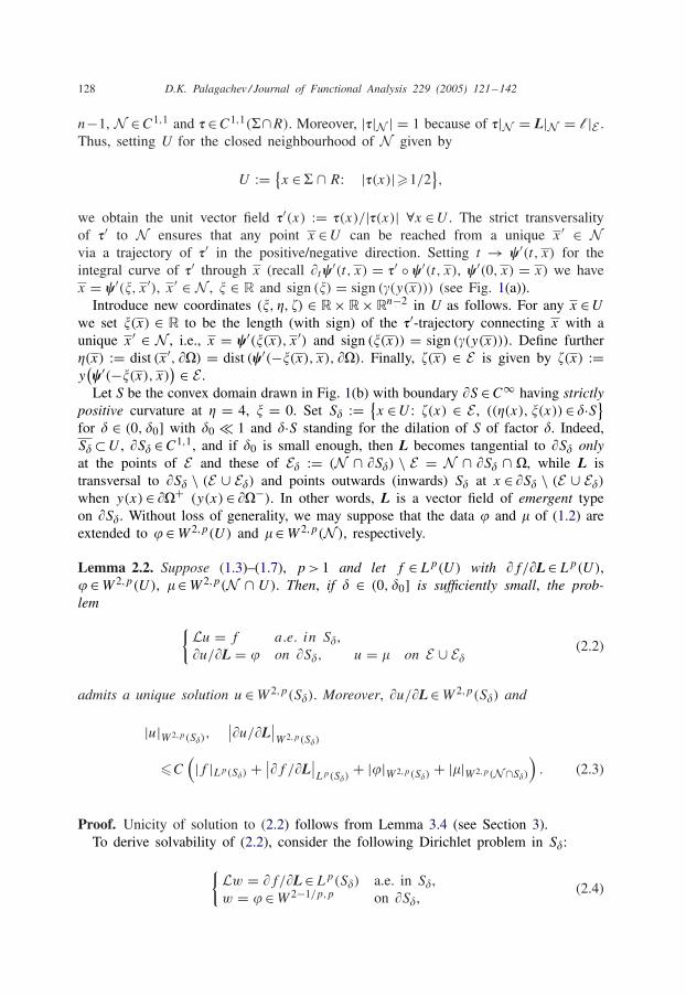
128 D.K. Palagachev / Journal of Functional Analysis 229 (2005) 121–142
n−1, N ∈ C1,1 and � ∈ C1,1(�∩R). Moreover, |�|N | = 1 because of �|N = L|N = l|E .Thus, setting U for the closed neighbourhood of N given by
U := {x ∈ � ∩ R: |�(x)|�1/2
},
we obtain the unit vector field �′(x) := �(x)/|�(x)| ∀x ∈ U . The strict transversalityof �′ to N ensures that any point x ∈ U can be reached from a unique x′ ∈ Nvia a trajectory of �′ in the positive/negative direction. Setting t → �′(t, x) for theintegral curve of �′ through x (recall �t�
′(t, x) = �′ ◦ �′(t, x), �′(0, x) = x) we havex = �′(�, x′), x′ ∈ N , � ∈ R and sign (�) = sign (�(y(x))) (see Fig. 1(a)).
Introduce new coordinates (�, �, ) ∈ R × R × Rn−2 in U as follows. For any x ∈ U
we set �(x) ∈ R to be the length (with sign) of the �′-trajectory connecting x with aunique x′ ∈ N , i.e., x = �′(�(x), x′) and sign (�(x)) = sign (�(y(x))). Define further�(x) := dist (x′, ��) = dist (�′(−�(x), x), ��). Finally, (x) ∈ E is given by (x) :=y(�′(−�(x), x)
) ∈ E .Let S be the convex domain drawn in Fig. 1(b) with boundary �S ∈ C∞ having strictly
positive curvature at � = 4, � = 0. Set S� := {x ∈ U : (x) ∈ E , ((�(x), �(x)) ∈ �·S}
for � ∈ (0, �0] with �0 � 1 and �·S standing for the dilation of S of factor �. Indeed,S� ⊂ U , �S� ∈ C1,1, and if �0 is small enough, then L becomes tangential to �S� onlyat the points of E and these of E� := (N ∩ �S�) \ E = N ∩ �S� ∩ �, while L istransversal to �S� \ (E ∪ E�) and points outwards (inwards) S� at x ∈ �S� \ (E ∪ E�)
when y(x) ∈ ��+ (y(x) ∈ ��−). In other words, L is a vector field of emergent typeon �S�. Without loss of generality, we may suppose that the data � and � of (1.2) areextended to � ∈ W 2,p(U) and � ∈ W 2,p(N ), respectively.
Lemma 2.2. Suppose (1.3)–(1.7), p > 1 and let f ∈ Lp(U) with �f/�L ∈ Lp(U),� ∈ W 2,p(U), � ∈ W 2,p(N ∩ U). Then, if � ∈ (0, �0] is sufficiently small, the prob-lem {
Lu = f a.e. in S�,�u/�L = � on �S�, u = � on E ∪ E�
(2.2)
admits a unique solution u ∈ W 2,p(S�). Moreover, �u/�L ∈ W 2,p(S�) and
|u|W 2,p(S�),
∣∣�u/�L∣∣W 2,p(S�)
�C(|f |Lp(S�) + ∣∣�f /�L
∣∣Lp(S�)
+ |�|W 2,p(S�)+ |�|W 2,p(N∩S�)
). (2.3)
Proof. Unicity of solution to (2.2) follows from Lemma 3.4 (see Section 3).To derive solvability of (2.2), consider the following Dirichlet problem in S�:{
Lw = �f/�L ∈ Lp(S�) a.e. in S�,w = � ∈ W 2−1/p,p on �S�,
(2.4)

D.K. Palagachev / Journal of Functional Analysis 229 (2005) 121–142 129
which, in view of the Lp-theory of uniformly elliptic operators (see [2,5]), admits aunique solution w ∈ W 2,p(S�).
To proceed further, consider the action of the operator L on the functions defined inU, which are constant on almost every trajectory of the field L. This defines a second-order operator L′ on the manifold N , which is uniformly elliptic with a constant�′ = �′(�, E, L, L) because of the strict transversality of L to N (a local representationof L′ is given at the proof of Theorem 3.3 below). Later, each point x ∈ U can bereached from x′ ∈ N through an L-trajectory (see Fig. 1(a)). Thus, setting t → �(t, x)
for the parameterization of the L-curve through x, for each x ∈ U , there exists a uniquevalue s(x) ∈ C1,1(U) of the parameter such that �(−s(x), x) = x′ ∈ N and withoutloss of generality we may assume |s(x)|�� ∀x ∈ S�. Now, for any x′ ∈ N define thetrace of f on N along the L-trajectories
f (x′) := f (x) −∫ s(x)
0
�f
�L◦ �(t, x′) dt, x ∈ U. (2.5)
It follows from Remark 2.1 that f is well-defined on N and f ∈ Lp(N ).Set N� := N ∩ S� and consider the Dirichlet problem
{L′v = f ∈ Lp(N�) a.e. in N�,v = � ∈ W 2−1/p,p on E ∪ E�
(2.6)
which has a unique solution v ∈ W 2,p(N�) in view of the uniform ellipticity of L′.Finally, for a.a. x ∈ S� define
u(x) := v ◦ �(−s(x), x) +∫ s(x)
0w ◦ �(t − s(x), x) dt
= v(x′) +∫ s(x)
0w ◦ �(t, x′) dt. (2.7)
Obviously, u satisfies the boundary conditions in (2.2) and, keeping in mind the regu-larity of v, w, �(·, ·) and s(x), we have
|Lu|Lp(S�),
∣∣∣∣�(Lu)
�L
∣∣∣∣Lp(S�)
�C(|f |Lp(N�) + ∣∣�f /�L
∣∣Lp(S�)
+ |�|W 2,p(S�)+ |�|W 2,p(N�)
)by means of the Lp-estimates for solutions to (2.4) and (2.6). Therefore, subtracting afunction of the type (2.7), we may consider hereafter (2.2) with homogeneous boundarydata � ≡ 0 and � ≡ 0.

130 D.K. Palagachev / Journal of Functional Analysis 229 (2005) 121–142
Let Hp be the linear space{f ∈ Lp(S�): �f /�L ∈ Lp(S�)
}equipped with the norm
‖f ‖Hp := |f |Lp(N�) + �1−1/p∣∣�f /�L
∣∣Lp(S�)
.
Trace (2.5) is uniquely defined by f and �f/�L and therefore ‖ · ‖Hp is a norm underwhich Hp becomes a Banach space.
We define now the operator A: Hp → Hp as Af := Lu, where u is given by (2.7)with v and w solutions to (2.4) and (2.6), respectively, with � ≡ 0 and � ≡ 0. Our aimwill be to show that A = IdHp + K + F with a compact operator K and a mapping Fwhose norm becomes small when � is small enough. For considering the differentialoperators
L1 :=(akj (x)DkjL
i(x))
Di, L2 :=(
2akj (x)DkLi(x) − Dka
ij (x)Lk(x))
Dij
with L∞-coefficients, it is clear that the commutator[L, �
�L
]= L �
�L− �
�LL equals
L1 + L2 whence
L1u + L2u = Lw − �(Lu)/�L a.e. S�.
An integration along the L-trajectory through x ∈ S� gives
Lu(x) = Lu(x′) +∫ s(x)
0(Lw − L1u − L2u) ◦ �(t, x′) dt
= Lu(x′) +∫ s(x)
0
�f
�L◦ �(t, x′) dt −
∫ s(x)
0(L1u + L2u) ◦ �(t, x′) dt
as consequence of (2.4), with x′ = �(−s(x), x) ∈ N�. Later on, (2.7) implies that
Lu(x) = L′v(x′) + L′1w(x) +
∫ s(x)
0(L′
2w) ◦ �(t, x′) dt a.a. x ∈ S�,
where L′i , i = 1, 2, is a differential operator of order i. Thus, setting T for the trace
operator T : W 1,p(S�) → Lp(N�) we get Lu(x′) = L′v(x′) + (T ◦ L′1w)(x′) whence
Lu(x′) = f (x′) + (T ◦ L′1w)(x′) = f (x) −
∫ s(x)
0
�f
�L◦ �(t, x′) dt + (T ◦ L′
1w)(x′)

D.K. Palagachev / Journal of Functional Analysis 229 (2005) 121–142 131
as follows from (2.6) and (2.5). Therefore
Lu(x) = f (x) + (T ◦ L′1w)(x′) −
∫ s(x)
0(L1u) ◦ �(t, x′) dt︸ ︷︷ ︸
=:Kf (x)
−∫ s(x)
0(L2u) ◦ �(t, x′) dt︸ ︷︷ ︸
=:Ff (x)
.
Before proceeding further, we point out that for each x′ ∈ N� the L-trajectory throughx′ intersects �S� at exactly two points x± such that �(s(x±), x′) = x±, s(x±)><0.Then 0 < s(x′) := s(x+) − s(x−)�2�. This way, for any function g ∈ L1(S�), Fubini’stheorem yields
∫S�
g(x) dx =∫
N�
dx′∫ s(x+)
s(x−)
g ◦ �(t, x′) dt.
With this tool at hand, it is easy to verify that
∣∣∣∣∣∫ s(x)
0g ◦ �(t, x′) dt
∣∣∣∣∣Lp(S�)
�21/p�|g|Lp(S�) ∀g ∈ Lp(S�) (2.8)
by Jensen’s integral inequality and s(x)��. Further, thinking of f in (2.5) as a functionextended from N� as constant on the L-curve through any x′ ∈ N�, we get
|f |Lp(S�) = |s(x′)1/pf (x′)|Lp(N�) �C(|f |Lp(S�) + �
∣∣�f /�L∣∣Lp(S�)
). (2.9)
Claim 2.1. K is a compact operator for any fixed � ∈ (0, �0].For,
|Kf |Lp(N�) = ∣∣T ◦ L′1w
∣∣Lp(N�)
�C∣∣L′
1w∣∣W 1,p(S�)
�C |w|W 2,p(S�)�C
∣∣�f /�L∣∣Lp(S�)
as a consequence of the Lp-estimates for (2.4) and the continuity of the trace operatorT . Further, using (2.8), (2.9) and s(x′)�2��2�0, we get
∣∣∣∣ ��L
(Kf )
∣∣∣∣Lp(S�)
� C
⎛⎝|L1v|Lp(S�)+ |w|Lp(S�)
+∣∣∣∣∣∫ s(x)
0L1w ◦ �(t, x′) dt
∣∣∣∣∣Lp(S�)
⎞⎠� C
(�1/p |L1v|Lp(N�)
+ |w|Lp(S�)+ � |L1w|Lp(S�)
)� C
(�1/p |v|W 1,p(N�)
+ |w|W 1,p(S�)
)

132 D.K. Palagachev / Journal of Functional Analysis 229 (2005) 121–142
� C(�1/p |v|W 2,p(N�)
+ |w|W 2,p(S�)
)� C
(�1/p|f |Lp(N�) + ∣∣�f /�L
∣∣Lp(S�)
).
This way,
‖Kf ‖Hp= |Kf |Lp(N�) + �1−1/p
∣∣�(Kf )/�L∣∣Lp(S�)
� C(∣∣T ◦ L′
1w∣∣Lp(N�)
+ � |v|W 1,p(N�)+ �1−1/p |w|W 1,p(S�)
)� C
(|w|W 2,p(S�)
+ � |v|W 2,p(N�)+ �1−1/p |w|W 2,p(S�)
)� C max{�−1+1/p, �, 1}‖f ‖Hp . (2.10)
Therefore, Kf ∈ Hp for any fixed � ∈ (0, �0]. To get the desired compactness ofK: Hp → Hp, we let {f�} to be a bounded sequence in Hp. It then follows, bymeans of the Lp-estimates for (2.6) and (2.4), that the sequences {v�} and {w�} ofrespective solutions are bounded in W 2,p(N�) and W 2,p(S�), respectively. In viewof the compactness of the imbedding W 2,p ↪→ W 1,p, there will be convergent (inW 1,p) subsequences, still denoted by {v�} and {w�}. Moreover, {L′
1w�} is bounded inW 1,p(S�) and therefore {T ◦L′
1w�(x′)} converges in Lp(N�) because the trace operator
T : W 1,p(S�) → Lp(N�) is compact (cf. [10]). This way, (2.10) gives∥∥K(f�−f)∥∥
Hp
�C( ∣∣(T ◦L′
1)(w�−w)∣∣Lp(N�)
+ ∣∣v�−v∣∣W 1,p(N�)
+ ∣∣w�−w∣∣W 1,p(S�)
).
Since the right-hand side above tends to 0 as �, → 0, {Kf�} is a Cauchy sequencein Hp and therefore convergent in the norm ‖ · ‖Hp . This proves the compactness ofK: Hp → Hp for any fixed � ∈ (0, �0].
Claim 2.2. ‖F‖Hp → Hp < 1 for � small enough.
Recall the definition of F , estimates (2.8) and (2.9) and |s(x)|��. Then Ff = 0and
‖Ff ‖Hp= �1−1/p
∣∣�(Ff )/�L∣∣Lp(S�)
= �1−1/p |L2u|Lp(S�)
� C�1−1/p
⎛⎝|L2v|Lp(S�)+ |w|W 1,p(S�)
+∣∣∣∣∣∫ s(x)
0L2w ◦ �(t, x′) dt
∣∣∣∣∣Lp(S�)
⎞⎠� C�1−1/p
(�1/p |L2v|Lp(N�)
+ |w|Lp(S�)+ |Dw|Lp(S�)
+ � |L2w|Lp(S�)
)

D.K. Palagachev / Journal of Functional Analysis 229 (2005) 121–142 133
� C(� |v|W 2,p(N�)
+ �1−1/p(|w|Lp(S�)
+ |Dw|Lp(S�)+ �|D2w|Lp(S�)
))� C�
(|f |Lp(N�) + �−1/p
(|w|Lp(S�)
+ |Dw|Lp(S�)+ �|D2w|Lp(S�)
)).
(2.11)
We used here the Lp-estimates for v in N�, taking into account that N� ∈ C1,1 uniformlyin �. It is not, however, the case concerning the terms depending on w. In fact, �S� isC1,1-smooth but the C1,1-norms of the diffeomorphisms which flatten locally �S� arenot uniformly bounded in � and one needs precise control on these. For this goal, weapply a rescaling argument. Remembering (2.4), define �−1·S� := {y ∈ Rn: �y ∈ S�}and thus �(�−1·S�) ∈ C1,1 uniformly in � in view of the definition of S�. Further,W(y) := w(�y) ∈ W 2,p(�−1·S�) is a strong solution to the Dirichlet problem
{Aij (y)Dyiyj
W = �2G(y) a.e. �−1·S�
W = 0 on �(�−1·S�),(2.12)
with Aij (y) := aij (�y), G(y) := �f/�L(�y). The Lp-estimates for (2.12) yield
|W |W 2,p(�−1·S�)
�C(n, p, �S)|�2G|Lp(�−1·S�)
,
whence, careful calculation of the seminorms involved gives
|w|Lp(S�)+ � |Dw|Lp(S�)
+ �2|D2w|Lp(S�) �C�2∣∣�f /�L
∣∣Lp(S�)
.
This way,
�−1/p(|w|Lp(S�)
+ |Dw|Lp(S�)+ �|D2w|Lp(S�)
)�C(2 + �0)�
1−1/p∣∣�f /�L
∣∣Lp(S�)
with a constant C independent of �, and (2.11) reads
‖Ff ‖Hp �C�‖f ‖Hp .
Therefore, the norm of the mapping F : Hp → Hp will be less than 1 if � is smallenough.
It follows from Claim 2.2 that IdHp + F is an invertible operator and since K iscompact, the Fredholm alternative asserts dim ker (A) = dim coker (A). Therefore, Ais an operator of full range im (A) ≡ Hp if and only if ker (A) = {0}. The triviality ofthe null-space ker (A), however, is obvious. In fact, supposing 0 �= f ∈ ker (A), we willhave Lu = Af = 0 a.e. S� and since �u/�L = 0 on �S�, u|E∪E� = 0, the uniquenessassertion (see Lemma 3.4 below) implies u ≡ 0 in S�. This way, w = �u/�L = 0 a.e.

134 D.K. Palagachev / Journal of Functional Analysis 229 (2005) 121–142
S�, v = u|N� = 0 whence �f/�L = Lw = 0 a.e. S�, f |N� = L′v = 0 a.e. N� andtherefore f = 0. This contradiction shows ker (A) = {0}.
To complete the proof of Lemma 2.2, we should only mention that ker (A) = {0} andim (A) = Hp give that the inverse mapping A−1: Hp → Hp is well defined. Thus, forany f ∈ Hp the unique solution of (2.2) is given by formula (2.7) with v and w solutionsof (2.6) and (2.4) with right-hand sides A−1f |N� and �(A−1f )/�L, respectively. �
3. Uniqueness and improving of summability
We postponed up to this point the treatment of unicity in W 2,p(�), ∀p > 1, ofsolutions to (1.2) because some of the constructions already used in Section 2 will beemployed. Let us start with the simpler case p > n/2.
Proposition 3.1. Suppose (1.3)–(1.6), p > n/2 and let u ∈ W 2,p(�) satisfy Lu = 0 a.e.in �, Bu = 0 on ��. Then u ∈ C0(�) ∩ W
2,nloc (�) ∩ C1,�(� \ E) ∀� ∈ (0, 1).
Proof. Indeed, u ∈ C0(�) as a consequence of (1.5), p > n/2 and Sobolev’s imbeddingW 2,p(�) ↪→ C0(�). Moreover, Lu = 0 ∈ Lq(�) ∀q ∈ (1, +∞) and the elliptic interiorregularity theory implies u ∈ W
2,q
loc (�). In particular, u ∈ W2,nloc (�). Further on, �u/�l =
0 ∈ W 2−1/q,q(��) ∀q ∈ (1, +∞) and l is transversal to �� away from E . Then theLp-theory of regular oblique derivative problem (cf. [2] if aij ∈ C0(�) and [12,13] ifaij ∈ V MO(�)) gives u ∈ W 2,q(�′) ∀q ∈ (1, +∞), ∀�′ ⊂ �\E , whence u ∈ C1,�(�\E)
∀� ∈ (0, 1) by means of Morrey’s lemma [5, Theorem 7.17]. �
Lemma 3.2. Suppose (1.3)–(1.7), p > n/2 and let u ∈ W 2,p(�) solve the homogeneousproblem (1.2): Lu = 0 a.e. �, Bu = 0 on ��, u = 0 on E . Then u ≡ 0.
Proof. We argue by contradiction. In view of Proposition 3.1, u ∈ C0(�) and supposingu(x) attains positive values in � we set u(x0) = max� u(x) > 0. Indeed, x0 /∈ E .Assuming x0 ∈ �, we obtain u = c = const in � by the Aleksandrov strong interiormaximum principle [5, Theorem 9.6] and Proposition 3.1. However, u = 0 on E whencec = 0 and therefore x0 /∈ �. Finally, suppose x0 ∈ �� \ E . Then Proposition 3.1 gives�u/�l ∈ C0(��\E) while l(x0) ·�(x0)
><0 if x0 ∈ ��±. Thus, the boundary point lemma
(see [5, Lemma 3.4]) would imply �u/�l(x0)>< 0 if x0 ∈ ��± which contradicts the
boundary condition. Therefore, u�0 in �.In the same manner, one gets u�0 in � whence u ≡ 0. �
To extend Lemma 3.2 to the case p ∈ (1, n/2] we note, first of all, that p > n/2ensures continuity of u in � and thus a possibility to apply maximum principle ar-guments. When dealing with non-degenerate BVPs, one derives firstly regularizationproperties of the BVP under consideration (i.e., higher regularity of the data implies

D.K. Palagachev / Journal of Functional Analysis 229 (2005) 121–142 135
higher regularity of solution) ensuring this way the necessary smoothness of solu-tion to the homogeneous BVP and then relies on maximum principle. It is not, how-ever, the case of the degenerate BVP (1.2). In fact, due to the “loss of smooth-ness” near E and the limited regularity of coefficients there is no, generally, hopeof success in that undertaking. However, as the next result shows, higher summabil-ity of the data in (1.2) implies higher summability of the solution and that is allwe need.
Theorem 3.3 (Improving-of-summability). Assume (1.3)–(1.7), 1 < p�q < + ∞ andlet u ∈ W 2,p(�) be a strong solution to (1.2) with f ∈ Lq(�), �f/�L ∈ Lq(�), � ∈W 1−1/q,q(��) ∩ W 2−1/q,q(�� ∩ �), � ∈ W 2−1/q,q(E). Then u ∈ W 2,q(�).
Proof. The improving-of-summability away from E follows just as in Proposition 3.1and is a consequence of the Lp-regularity theory of non-degenerate oblique derivativeproblems [12,13]. In other words, u ∈ W 2,q(�′) ∀�′ ⊂ � \ E and in order to de-rive Theorem 3.3 it suffices to show u ∈ W 2,q(�). For, setting v := �u/�L ∈ W 1,p(�)
and taking the difference quotients in L-direction of the equation in (1.2) we re-alize that v ∈ W 2,p(�) (cf. [5, Lemma 7.24]) and it locally solves the Dirichletproblem
⎧⎨⎩ aij (x)Dij v = �f/�L − DkaijDijuLk
+2aijDkiuDjLk + aijDkuDijL
k ∈ Lp(�) a.e. �v = � on �� ∩ �.
(3.1)
Indeed, u ∈ W 2,q(�′) ∀�′ ⊂ � \ E and therefore the right-hand side of the equation in(3.1) belongs to Lq(�′) whence v ∈ W 2,q(�′). To get the same regularity of u and v
near the set of tangency E , we recall that for any x ∈ S� one has (cf. (2.5))
u(x) = u(x′) +∫ s(x)
0v ◦ �(t, x′) dt, x′ ∈ N�, x = �(s(x), x′), (3.2)
where u is the trace of u on N� along the L-trajectories. It follows from Remark 2.1that u ∈ W 2,p(N�). Let x′
0 ∈ N� be an arbitrary point. Since the fields L are strictlytransversal to N� there exist an n-dimensional neighbourhood O of x′
0 and a C1,1-diffeomorphism which straightens L in O such that �/�L ≡ �/�xn with respect to anew coordinate system centred at x′
0. Moreover, N� ∩O admits the local representationxn = �(x) for each x = (x1, . . . , xn−1) belonging to a neighbourhood O of the originin Rn−1. Then
Lu ≡n−1∑i,j=1
aij (x)Diju +n−1∑i=1
ain(x)Di
(��L
u
)+ ann(x)
��L
(��L
u
)a.e. S� ∩ O
136 D.K. Palagachev / Journal of Functional Analysis 229 (2005) 121–142
and taking traces on N� ∩ O along the L-curves leads to
L′u :=n−1∑i,j=1
aij (x, �(x))Dij u = F := f −n−1∑i=1
ain(x, �(x))Div − ann(x, �(x))˜�v/�L
+n−1∑i=1
Ai(x, �(x))Div + A(x, �(x))v a.a. (x, �(x)) ∈ N� ∩ O
with suitable Ai, A ∈ L∞(N� ∩ O). We have f, �f/�L ∈ Lq(�) and thusf ∈ Lq(N�) (cf. (2.5) and Remark 2.1). Further, v ∈ W 2,p(S�), Dv ∈ W 1,p(S�) whence
v, Div, ˜�v/�L ∈ Lr(N� ∩O) with r = (n−1)p/(n−p) if p < n and any r > 1 if p�n
(see [1, Lemma 5.19; 10, Theorems 6.4.1, 6.4.2]). Therefore, − ∑n−1i=1 ain(x, �(x))
Div−ann(x, �(x))˜�v/�L+∑n−1i=1 Ai(x, �(x))Div+A(x, �(x))v ∈ Lr(N�∩O) and thus
F ∈ Lq ′(N� ∩ O) with q ′ = min{q, (n − 1)p/(n − p)} if p < n and q ′ = q otherwise.
Anyway, q ′ > p and
{L′u = F ∈ Lq ′
(N�) a.e. N� ∩ O,
u = � ∈ W 2−1/q,q(E) on E ∩ O, u ∈ W 2−1/q,q(E�) on E� ∩ O,
whence u ∈ W 2,q ′(N� ∩ O). In view of the arbitrariness of the point x′
0, we conclude
that u ∈ W 2,q ′(N�).
To get increasing of summability for v, we differentiate twice (3.2) and substitutethe derivatives of u into the right-hand side of (3.1), obtaining this way
aij (x)Dij v = F(x) +∫ s(x)
0(P2v) ◦ �(t, x′) dt,
with F(x) := �f/�L + P2u + P1v. Here Pi , i = 1, 2, is a differential operatorof order i with L∞-coefficients, while P2 is a second-order operator on N�. Thus,P2u ∈ Lq ′
(S�) (after extension of u in S� as constant along any L-curve through N�),P1v ∈ W 1,p(S�) ↪→ Lr(S�) with r = np/(n−p) if p < n and any r > 1 if p�n. There-fore, F ∈ Lq ′′
(S�) with q ′′ = min{q ′, np/(n − p)} if p < n and q ′′ = q ′ otherwise.Indeed, q ′′ = q ′ > p and thus v ∈ W 2,p(S�) solves the non-local Dirichlet problem
{Lv = F(x) + ∫ s(x)
0 (P2v) ◦ �(t, x′) dt a.e. S�, F ∈ Lq ′(S�),
v = � ∈ W 2−1/q,q on �S� ∩ ��, v ∈ W 2−1/q,q on �S� \ ��.
(3.3)
We claim now that v ∈ W 2,q ′(S�) for � small enough. In fact, take any r ∈ [p, q ′] and
define the operator C: W 2,r (S�) → W 2,r (S�) as follows: for each w ∈ W 2,r (S�) the

D.K. Palagachev / Journal of Functional Analysis 229 (2005) 121–142 137
image Cw is the unique solution Cw ∈ W 2,r (S�) of the Dirichlet problem
{L(Cw) = F(x) + ∫ s(x)
0 (P2w) ◦ �(t, x′)dt ∈ Lr(S�) a.e. S�,
Cw = � ∈ W 2−1/q,q on �S� ∩ ��, Cw = v ∈ W 2−1/q,q on �S� \ ��.
We shall prove that C is a contraction for small �. For, taking arbitrary w1, w2 ∈W 2,r (S�) one has
{L(Cw1 − Cw2) = ∫ s(x)
0 (P2w1 − P2w2) ◦ �(t, x′) dt a.e. S�,
Cw1 − Cw2 = 0 on �S�
and rescaling arguments similar to those already used (see (2.12)) give
|Cw1 − Cw2|W 2,r (S�)�C
∣∣∣∣∣∫ s(x)
0(P2w1 − P2w2) ◦ �(t, x′) dt
∣∣∣∣∣Lr(S�)
with C depending on known quantities and �0, but not on �. It follows (cf. (2.8)) that
|Cw1 − Cw2|W 2,r (S�)�C� |P2(w1 − w2)|Lr(S�)
�C� |w1 − w2|W 2,r (S�)
and therefore C will be really a contraction from W 2,r (S�) into itself if � is smallenough. Then C admits a unique fixed point in W 2,r (S�) for each r ∈ [p, q ′] and sincev ∈ W 2,p(S�) is already a fixed point (note that v solves (3.3)!), we get v ∈ W 2,r (S�)
∀r ∈ [p, q ′]. Thus v ∈ W 2,q ′(S�), u ∈ W 2,q ′
(N�) and therefore (3.2) yields u ∈ W 2,q ′(S�)
with q ′ > p.To complete the proof of Theorem 3.3 it remains to iterate the above procedure
finitely many times with q ′ instead of p until q ′ becomes equal to q. �
We are in a position now to generalize Lemma 3.2 for all values p > 1.
Lemma 3.4. Let p ∈ (1, +∞) and suppose (1.3)–(1.7). Let u ∈ W 2,p(�) solve thehomogeneous problem (1.2): Lu = 0 a.e. �, Bu = 0 on ��, u = 0 on E . Then u ≡ 0in �.
Proof. Theorem 3.3 assures u ∈ W 2,q(�) for any q > 1. The statement of Lemma 3.4then follows by choosing q > n/2 and employing Lemma 3.2. �
4. Solvability of (1.2) away from E
Hereafter � > 0 will be a fixed number for which Lemma 2.2 holds true.

138 D.K. Palagachev / Journal of Functional Analysis 229 (2005) 121–142
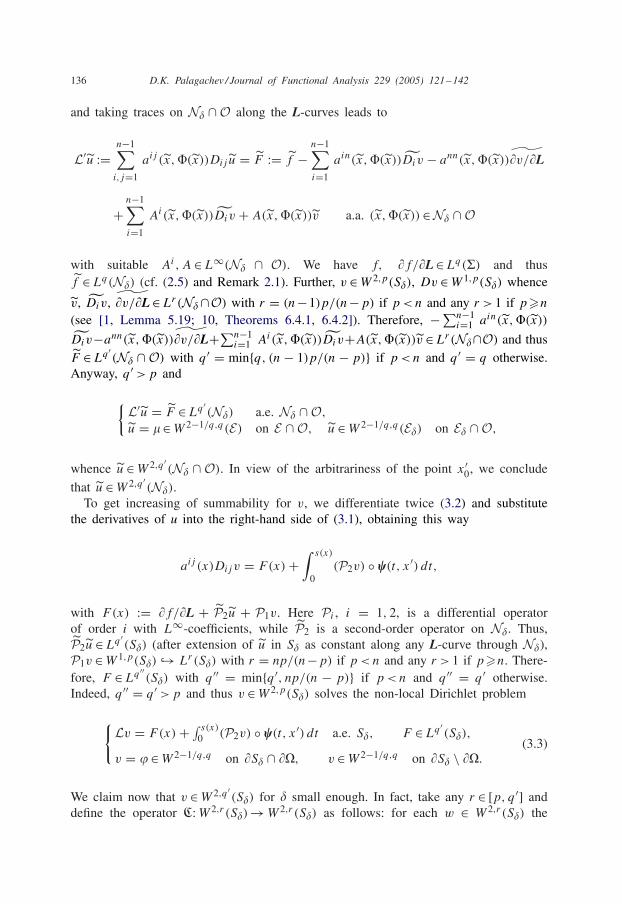
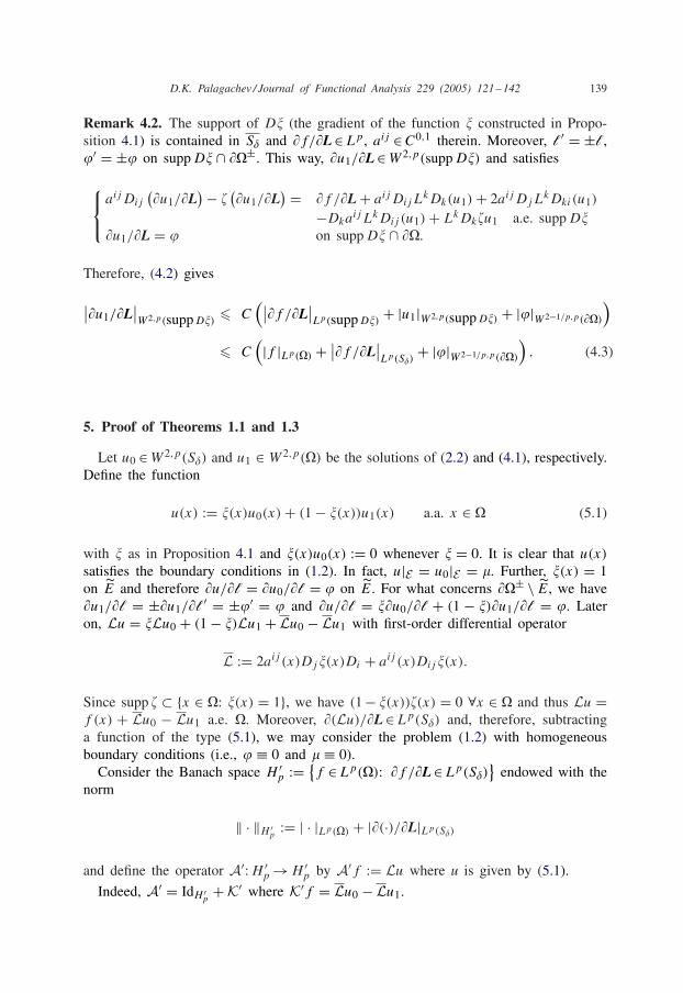
Fig. 2. The graphs of �∈ C∞(R) and ∈ C∞0 (−3�/4, 3�/4).
Proposition 4.1. There exists a cut-off function � ∈ C1,1(�), such that supp � ⊂ S�,��/�L = 0 in S�, 0���1 and � ≡ 1 in a neighbourhood of E in �.
Proof. Define �: N� → R on the manifold N� such that 0���1, � ≡ 1 in a smallneighbourhood of E in N� while � ≡ 0 in a large enough neighbourhood of E�.Extend � to S� as constant on the L-curve through any point of N� and set � := 0 in� \ S�. �
Let E ⊂ {x ∈ ��: �(x) = 1} ⊂ U ∩ �� be a neighbourhood of E in �� suchthat |�|�1/4 there. (Recall that U is a closed neighbourhood of N in � ∩ R where|�(x)|�1/2, see Section 2.) Then any point x ∈ U ∩ �� can be reached from somex′ ∈ E along a trajectory of the field �′ = �/|�|. Setting, as before, t → �′(t, x) forthe parameterization of the maximal �′-curve through x, we have s(x) ∈ C1,1(U ∩ ��),where �′(−s(x), x) = x′ ∈ E . Let � := minx∈(U∩��)\E |s(x)| > 0 and consider thefunctions � ∈ C∞(R) and ∈ C∞
0 (−3�/4, 3�/4) with plots drawn in Fig. 2.Define
l′(x) :=⎧⎨⎩ l(x), x ∈ ��+ \ E,
�(s(x))l(x) + (s(x))�(x), x ∈ E,−l(x), x ∈ ��− \ E,
�′(x) := �(x)( ± �(x)
), x ∈ ��±,
where � ∈ C∞(��) is a cut-off function with � ≡ 0 in a neighbourhood E′ of E in ��,E′ ⊂ E, � ≡ 1 on �� \ E. Finally, take ∈ C∞(�) with supp ⊂ {x ∈ �: �(x) = 1},�0 and consider the regular oblique derivative problem{
(L − (x))u1 = f ∈ Lp(�) a.e. �,�u1/�l′ = �′ on ��,
(4.1)
which possesses a unique solution u1 ∈ W 2,p(�) (see [13] and note that the field l′ isstrictly transversal to ��.) Moreover,
|u1|W 2,p(�) �C(|f |Lp(�) + |�′|W 1−1/p,p(��)
)�C
(|f |Lp(�) + |�|W 2−1/p,p(��)
). (4.2)
D.K. Palagachev / Journal of Functional Analysis 229 (2005) 121–142 139
Remark 4.2. The support of D� (the gradient of the function � constructed in Propo-sition 4.1) is contained in S� and �f/�L ∈ Lp, aij ∈ C0,1 therein. Moreover, l′ = ±l,�′ = ±� on supp D� ∩ ��±. This way, �u1/�L ∈ W 2,p(supp D�) and satisfies
⎧⎨⎩ aijDij
(�u1/�L
) − (�u1/�L
) = �f /�L + aijDijLkDk(u1) + 2aijDjL
kDki(u1)
−DkaijLkDij (u1) + LkDku1 a.e. supp D�
�u1/�L = � on supp D� ∩ ��.
Therefore, (4.2) gives
∣∣�u1/�L∣∣W 2,p(supp D�)
� C(∣∣�f /�L
∣∣Lp(supp D�)
+ |u1|W 2,p(supp D�) + |�|W 2−1/p,p(��)
)� C
(|f |Lp(�) + ∣∣�f /�L
∣∣Lp(S�)
+ |�|W 2−1/p,p(��)
). (4.3)
5. Proof of Theorems 1.1 and 1.3
Let u0 ∈ W 2,p(S�) and u1 ∈ W 2,p(�) be the solutions of (2.2) and (4.1), respectively.Define the function
u(x) := �(x)u0(x) + (1 − �(x))u1(x) a.a. x ∈ � (5.1)
with � as in Proposition 4.1 and �(x)u0(x) := 0 whenever � = 0. It is clear that u(x)
satisfies the boundary conditions in (1.2). In fact, u|E = u0|E = �. Further, �(x) = 1on E and therefore �u/�l = �u0/�l = � on E. For what concerns ��± \ E, we have�u1/�l = ±�u1/�l′ = ±�′ = � and �u/�l = ��u0/�l + (1 − �)�u1/�l = �. Lateron, Lu = �Lu0 + (1 − �)Lu1 + Lu0 − Lu1 with first-order differential operator
L := 2aij (x)Dj�(x)Di + aij (x)Dij�(x).
Since supp ⊂ {x ∈ �: �(x) = 1}, we have (1 − �(x))(x) = 0 ∀x ∈ � and thus Lu =f (x) + Lu0 − Lu1 a.e. �. Moreover, �(Lu)/�L ∈ Lp(S�) and, therefore, subtractinga function of the type (5.1), we may consider the problem (1.2) with homogeneousboundary conditions (i.e., � ≡ 0 and � ≡ 0).
Consider the Banach space H ′p := {
f ∈ Lp(�): �f /�L ∈ Lp(S�)}
endowed with thenorm
‖ · ‖H ′p
:= | · |Lp(�) + |�(·)/�L|Lp(S�)
and define the operator A′: H ′p → H ′
p by A′f := Lu where u is given by (5.1).
Indeed, A′ = IdH ′p
+ K′ where K′f = Lu0 − Lu1.

140 D.K. Palagachev / Journal of Functional Analysis 229 (2005) 121–142
Claim 5.1. K′: H ′p → H ′
p is a compact operator.
Note supp L ⊆ supp D� ⊂ S� and use (2.3) and (4.2) to obtain∣∣K′f∣∣Lp(�)
= |L(u0 − u1)|Lp(�) �C(|u0|W 1,p(S�)
+ |u1|W 1,p(�)
)� C
(|u0|W 2,p(S�)+ |u1|W 2,p(�)
)�C
(|f |Lp(�) + ∣∣�f /�L
∣∣Lp(S�)
).
Further, Proposition 4.1, (2.3), (4.2) and (4.3) give∣∣�(K′f )/�L∣∣Lp(S�)
� C( |u0|W 1,p(S�)
+ |u1|W 1,p(�) + ∣∣�(u0 − u1)/�L∣∣W 1,p(supp D�)
)� C
(|u0|W 2,p(S�)
+ |u1|W 2,p(�) + ∣∣�u0/�L∣∣W 2,p(S�)
+ ∣∣�u1/�L∣∣W 2,p(supp D�)
)� C
( |f |Lp(�) + ∣∣�f /�L∣∣Lp(S�)
)and the compactness of the imbedding W 2,p ↪→ W 1,p implies that K′ is a compactmapping.
Therefore, A′ = IdH ′p+K′ is a Fredholm operator and dim ker (A′) = dim coker (A′).
In particular, A′ will be of full range (im (A′) = H ′p) if and only if ker (A′) = {0}.
Claim 5.2. ker (A′) = {0}.
We argue by contradiction. Supposing there exists 0 �= f ∈ ker (A′), we have A′f =0 = Lu a.e. �. Moreover, �u/�l = 0 on ��, u|E = 0 and Lemma 3.4 implies that u ≡ 0in �. Since � ≡ 0 in � \ S�, (5.1) gives u1 = 0 there, whence f = (L − (x))u1 = 0a.e. � \ S�.
To get f = 0 a.e. S�, we will prove that u0 = u1 in S�. For, (5.1) and u ≡ 0 yieldu0 = 0 a.e. {x: �(x) = 1}. In particular, supp ⊂ {x: � = 1} and therefore (x)u0(x) = 0in {x: � = 1} and thus also in S� (note ≡ 0 on S� \ {x: � = 1}). Therefore,
(L − (x))(u1 − u0) = (L − (x))u1 − Lu0 + (x)u0 = 0 a.e. S�. (5.2)
We have �(x) = 0 and u1(x) = u(x) = 0 for x near �S� \ ��, whence
�(u1 − u0)/�L = 0 on �S� \ ��, u1 − u0 = 0 on E�. (5.3)
Further, �u0/�l = 0 on �S� ∩ �� whereas �u1/�l = ±�u1/�l′ on {x ∈ ��: l′ = ±l}and therefore
�(u1 − u0)/�l′ = 0 on {x ∈ ��: l′(x) = ±l(x)}. (5.4)

D.K. Palagachev / Journal of Functional Analysis 229 (2005) 121–142 141
Concerning {x ∈ ��: l′(x) �= ±l(x)}, there is a neighbourhood of this set fully con-tained in {x: � = 1}, and (5.1) gives u0 = 0 therein. Thus �u0/�l′ = 0 on {x ∈��: l′ �= l} and
�(u1 − u0)/�l′ = 0 on {x ∈ ��: l′(x) �= ±l(x)}. (5.5)
Now, arguing as in Lemma 3.4, (5.2)–(5.5) imply that u1 = u0 in S� whence u0 =u1 = 0 in S� as it follows from (5.1) and u ≡ 0 in �. Thus f = Lu0 = 0 in S�.
Therefore, f ≡ 0 in � and this proves the triviality of the null-space ker (A′).With Claims 5.1 and 5.2 at hand, the proof of Theorem 1.1 completes by the Fred-
holm alternative. In particular, since A′: H ′p → H ′
p is an invertible operator, the solutionof (1.2) will be given by (5.1), where u0 and u1 solve (2.2) and (4.1), respectively,with right-hand side A′−1
f .The proof of Theorem 1.3 follows that of Theorem 1.1 with the necessary modifi-
cations. Precisely, the operator A′: H ′p → H ′
p should be defined as A′f = Gu with u
given by (5.1). Thus A′ = IdH ′p+K′, where K′f = (
L+biDi�+�(biDi +c))u0 −(
L+biDi� + (1 − �)(biDi + c + )
)u1 and L as before. The compactness of K′: H ′
p → H ′p
ensures A′ is a Fredholm operator and therefore dim ker (A′) = dim coker (A′) < ∞with ker (A′) = {0} when c(x)�0 (note that Lemma 3.4 remains valid also for theoperator G with c(x)�0). The details are left to the reader.
Acknowledgments
The results presented here are an outgrowth of the author’s visit at Départementde Mathématiques, Université de Nantes, the beneficial academic atmosphere of whichis highly appreciated. Special credit is due to Georgi Vodev for the friendship andgratifying discussions.
References
[1] R. Adams, Sobolev Spaces, Academic Press, New York, 1975.[2] S. Agmon, A. Douglis, L. Nirenberg, Estimates near the boundary for solutions of elliptic partial
differential equations satisfying general boundary conditions I, Commun. Pure Appl. Math. 12 (1959)623–727; II, Commun. Pure Appl. Math. 17 (1964) 35–92.
[3] Y.V. Egorov, Linear Differential Equations of Principal Type, Contemporary Soviet Mathematics,New York, 1986.
[4] Y.V. Egorov, V. Kondrat’ev, The oblique derivative problem, Math. USSR Sbornik 7 (1969) 139–169.
[5] D. Gilbarg, N.S. Trudinger, Elliptic Partial Differential Equations of Second Order, second ed.,Springer, Berlin, 1983.
[6] P. Guan, E. Sawyer, Regularity estimates for the oblique derivative problem, Ann. Math. 137 (1993)1–70.
[7] P. Guan, E. Sawyer, Regularity estimates for the oblique derivative problem on non-smooth domainsI, Chinese Ann. Math. Ser. B 16 (3) (1995) 1–26; II, Chinese Ann. Math. Ser. B 17(1) (1996)1–34.

142 D.K. Palagachev / Journal of Functional Analysis 229 (2005) 121–142
[8] L. Hörmander, Pseudodifferential operators and non-elliptic boundary value problems, Ann. Math.83 (1966) 129–209.
[9] L. Hörmander, The Analysis of Linear Partial Differential Operators III: Pseudo-DifferentialOperators; IV: Fourier Integral Operators, Springer, Berlin, 1985.
[10] A. Kufner, O. John, S. Fucík, Function Spaces, Noordhoff, Leyden, 1977.[11] P.A. Martin, On the diffraction of Poincaré waves, Math. Methods Appl. Sci. 24 (2001) 913–925.[12] A. Maugeri, D.K. Palagachev, Boundary value problem with an oblique derivative for uniformly
elliptic operators with discontinuous coefficients, Forum Math. 10 (4) (1998) 393–405.[13] A. Maugeri, D.K. Palagachev, L.G. Softova, Elliptic and Parabolic Equations with Discontinuous
Coefficients, Wiley-VCH, Berlin, 2000.[14] A. Maugeri, D.K. Palagachev, C. Vitanza, A singular boundary value problem for uniformly elliptic
operators, J. Math. Anal. Appl. 263 (2001) 33–48.[15] V. Maz’ya, On a degenerating problem with directional derivative, Math. USSR Sbornik 16 (1972)
429–469.[16] V. Maz’ya, B.P. Paneah, Degenerate elliptic pseudodifferential operators and oblique derivative
problem, Trans. Moscow Math. Soc. 31 (1974) 247–305.[17] A. Melin, J. Sjöstrand, Fourier integral operators with complex phase functions and parametrix for
an interior boundary value problem, Commun. Partial Differential Equations 1 (1976) 313–400.[18] D.K. Palagachev, The tangential oblique derivative problem for second order quasilinear parabolic
operators, Commun. Partial Differential Equations 17 (1992) 867–903.[19] D.K. Palagachev, Lp-regularity for Poincaré problem and applications, in: F. Giannessi, A. Maugeri
(Eds.), Variational Analysis and Applications, 38th Workshop dedicated to the memory of GuidoStampacchia, Erice, Sicily, 20 June–1 July, 2003, Kluwer Academic Publishers, Dordrecht, TheNetherlands, 2004, pp. 773–789.
[20] D.K. Palagachev, The Poincaré problem in Lp-Sobolev spaces. II: full dimension degeneracy,submitted.
[21] B.P. Paneah, On a problem with oblique derivative, Soviet Math. Dokl. 19 (1978) 1568–1572.[22] B.P. Paneah, On the theory of solvability of the oblique derivative problem, Math. USSR Sbornik
42 (1982) 197–235.[23] B.P. Paneah, The Oblique Derivative Problem, The Poincaré Problem, Wiley-VCH, Berlin, 2000.[24] H. Poincaré, Lecons de Méchanique Céleste, Tome III, Théorie de Marées, Gauthiers–Villars, Paris,
1910.[25] P.R. Popivanov, N.D. Kutev, The tangential oblique derivative problem for nonlinear elliptic equations,
Commun. Partial Differential Equations 14 (1989) 413–428.[26] P.R. Popivanov, D.K. Palagachev, The Degenerate Oblique Derivative Problem for Elliptic and
Parabolic Equations, Akademie–Verlag, Berlin, 1997.[27] B. Winzell, The oblique derivative problem I, Math. Ann. 229 (1977) 267–278; II, Ark. Math. 17
(1979) 107–122.[28] B. Winzell, A boundary value problem with an oblique derivative, Commun. Partial Differential
Equations 6 (1981) 305–328.[29] Y. Zheng, A global solution to a two-dimensional Riemann problem involving shocks as free
boundaries, Acta Math. Appl. Sin. Engl. Ser. 19 (2003) 559–572.
[30] L.G. SZftova, W2,1p -solvability for the parabolic Poincaré probelm, Commun. Partial Differential
Equations 29 (11&12) (2004) 1783–1798.