The Poincar e polynomial for the - amslaurea.unibo.it
60
Alma Mater Studiorum · Universit ` a di Bologna SCUOLA DI SCIENZE Corso di Laurea Magistrale in Matematica The Poincar´ e polynomial for the Hilbert scheme of points of C 2 Tesi di Laurea Magistrale in Geometria Relatore: Chiar.mo Prof. Luca Migliorini Presentata da: Angelica Simonetti I Sessione Anno Accademico 2014-2015
Transcript of The Poincar e polynomial for the - amslaurea.unibo.it
Alma Mater Studiorum · Universita di Bologna
SCUOLA DI SCIENZE
Corso di Laurea Magistrale in Matematica
The Poincare polynomial for the
Hilbert scheme of points of C2
Tesi di Laurea Magistrale in Geometria
Relatore:Chiar.mo Prof.Luca Migliorini
Presentata da:Angelica Simonetti
I SessioneAnno Accademico 2014-2015

Se fossi accademico, fossi maestro o dottore,ti insignirei in toga di quindici lauree ad honorem,
ma a scuola ero scarso in latino e il pop non e fatto per me:ti diplomero in canti e in vino qui in via Paolo Fabbri 43
F.G.

Contents
Introduzione i
Introduction iii
1 Hilbert schemes, an overview 11.1 General results . . . . . . . . . . . . . . . . . . . . . . . . . . . . . . . 11.2 Hilbert schemes of points . . . . . . . . . . . . . . . . . . . . . . . . . . 2
1.2.1 Case X = A2 . . . . . . . . . . . . . . . . . . . . . . . . . . . . 51.3 Further facts and results . . . . . . . . . . . . . . . . . . . . . . . . . . 13
1.3.1 Framed moduli space of torsion free sheaves on P2 . . . . . . . . 131.3.2 Symplectic structure . . . . . . . . . . . . . . . . . . . . . . . . 151.3.3 The Douady space . . . . . . . . . . . . . . . . . . . . . . . . . 18
2 Hyper-Kahler metric on (C2)[n] 212.1 Geometric invariant theory quotients . . . . . . . . . . . . . . . . . . . 21
2.1.1 Geometric invariant theory and the moment map . . . . . . . . 232.1.2 Description of (C2)[n] as a GIT quotient . . . . . . . . . . . . . 25
2.2 Hyper-Kahler quotients . . . . . . . . . . . . . . . . . . . . . . . . . . . 27
3 The Poincare polynomial of (C2)[n] 333.1 Perfectness of the Morse function . . . . . . . . . . . . . . . . . . . . . 333.2 Case X = (C2)[n] . . . . . . . . . . . . . . . . . . . . . . . . . . . . . . 36
Ringraziamenti 47
Bibliografia 49


Introduzione
Dato uno schema quasi proiettivo X localmente Notheriano, possiamo pensare alloschema di Hilbert, Hilb(X), come ad uno spazio di moduli che parametrizza i sottos-chemi di X, tenendo in considerazione il loro polinomio di Hilbert. Se ad esempiofissiamo tale polinomio, considerandolo costante e uguale ad n, allora lo schema diHilbert che otteniamo, Hilbn(X) = X [n] parametrizza i sottoschemi 0-dimensionali diX di lunghezza n. L’esempio piu semplice di sottoschema zero dimensionale di questotipo e rappresentato dai sottoinsiemi di n punti distinti di X, ma certamente essi nonesauriscono tutte le possibilita: occorre infatti considerare i casi in cui gli n punti nonsono piu tutti distinti tra di loro, ed alcuni di essi coincidono e vengono contati conmolteplicita. Si vede dunque come la struttura di schema assuma rilevanza e conferiscaallo spazio una maggiore ricchezza.
Come sempre quando si trattano spazi di moduli, e di grande interesse studiare lepossibili strutture e proprieta degli schemi di Hilbert: talune vengono ereditate dallospazio X di partenza, ma ne potrebbero intervenire delle nuove, tipiche dello spaziodi moduli in esame. Per prima cosa, la costruzione funtoriale degli schemi di Hilbertfornita da Grothendieck, ci assicura che Hilb(X) sia sempre uno schema e, di piu, essoe proiettivo se X lo e. Inoltre se consideriamo il caso particolare di X [n], tale schemapuo essere dotato di una struttura simplettica, tutte le volte che X ne ha una; se poici limitiamo agli schemi X di dimensione 2, non singolari, allora e possibile dimostrareche X [n] e anch’esso non singolare ed il morfismo X [n] → SnX, risulta essere unarisoluzione delle singolarita del prodotto simmetrico.
Questo lavoro prende in esame il caso particolare in cui X = C2, considerandone loschema di Hilbert di punti. Piu nello specifico lo scopo della tesi e lo studio dei numeridi Betti di (C2)[n]: cio che si ottiene e una espressione del tipo serie di potenze, la qualee un caso particolare di una formula molto piu generale, nota con il nome di formula diGottsche. E interessante notare come tale formula descriva i numeri di Betti di tutti glischemi di Hilbert di punti di C2 considerati simultaneamente, in termini dei numeri diBetti di X. La formula di Gottsche compare anche in un contesto totalmente diverso,mostrando una connessione tra ambiti distinti dell’algebra e della geometria: se infatticonsideriamo un certo tipo di superalgebre infinito dimensionali, prodotto di algebre diHeisenberg e Clifford, e guardiamo alla loro formula dei caratteri, ritroviamo proprio
i
la formula di Gottsche.
La tesi e organizzata come segue. Nel primo capitolo introduciamo gli schemidi Hilbert concentrandoci sul caso di nostro interesse. Diamo una semplice ed utiledescrizione di (C2)[n] e ne esplorismo la strutture simplettica.Il secondo capitolo e invece dedicato alla descrizione di (C2)[n] come quoziente iperKahleriano: le varieta iper Kahleriane non sono facili da costruire, dunque da un latotale risultato ha valore in se, dall’altro sara utile per poter utilizzare la teoria di Morsenel capitolo successivo.Nel terzo capitolo infine determiniamo il polinimio di Poincare dello schema di Hilbertdi punti di C2, usando la teoria di Morse e l’azione naturale del toro su C2, insiemealla relativa mappa momento, che dimostreremo essere una funzione di Morse.
ii
Introduction
Given a quasi projective locally Notherian scheme X, the Hilbert scheme of X, Hilb(X)can be thought as the moduli space parametrizing the subschemes ofX, coherently withthe information provided by their Hilbert Polynomial. If we fix the Hilbert polynomialto be constant and equal to n (Hilbn(X) = X [n]), then we restrict our attention to the0-dimensional subschemes of X of length n. The simplest example of zero dimensionalsubschemes of this kind are the sets of n distinct points of X, but they of course do notrun out all the possibilities: some of these points may collide, in other words some ofthem may coincide and be counted with multiplicity and then the structure of schemebecomes relevant.
As always when we deal with moduli spaces, it is of great interest to study all thepossible structures and properties of the Hilbert schemes: some of them are inher-ited by the ones which exist on X, others can be typical of HilbP (X). First of all,Grothendieck’s construction of the Hilbert scheme implies that Hilb(X) is a schemeand it is projective if X is. Moreover if we consider X [n], it can equipped with a sym-plectic structure if X has one; finally if dimX = 2 and X is smooth, then X [n] hasparticularly mice properties: it is smooth, and the morphism X [n] → SnX turns outto be a resolution of singularities for the symmetric product.
This work is concerned with a very specific Hilbert scheme, which is the Hilbertscheme of points of C2; in particular our aim is to study the Betti numbers of (C2)[n]:we will obtain a power series expression, which is a particular case of a more generalformula, known as the Gottsche formula. The interesting fact is that it describes theBetti numbers of all the Hilbert schemes of points of C2 at once, in terms of the Bettinumbers of X. This formula is also important because appears in a very differentcontext, giving to us a striking connection between two fields that seem to be very far:indeed it coincide with the character formula for a representation of a type of infinitedimensional superalgebras, products of the Heisenberg and Clifford algebras.
The work is organized as follows. In the first chapter we introduce the Hilbertschemes, focusing on the case we are interested in. We give a useful description of(C2)[n] and explore the symplectic structure it is endowed with.The second chapter is devoted to describe (C2)[n] as an hyper-Kahler quotient: thehyper-Kahler manifolds are not so easy to construct, hence this result has an interest
iii

on its own, besides the hyper-Kahler structure will be needed after in order to applyMorse Theory .In the third chapter we finally determine the Poincare polynmial of the Hilbert schemeof points of C2 using Morse Theory and the natural torus action together with therelated moment map, which will be proved to be a Morse function.
iv
Chapter 1
Hilbert schemes, an overview
1.1 General results
In this section we give an introduction to Hilbert schemes, beginning with the generaldefinition: all schemes are supposed locally Notherian.
Definition 1.1. Let X be a projective scheme over an algebraically closed field K eOX(1) an ample line bundle. For every scheme S the functorHilbX is defined as follows:
HilbX(S) = Z ⊂ X × S, Z closed subscheme, Z flat over S
HilbX(S) is a controvariant functor from the category of Schemes over K to the oneof Sets which associates to each scheme S the set of families Z of closed subschemesZx ⊂ X parametrized by S, so that, if we look at the diagram
Z
π
i // X × S
pS
S= // S
the projection π is flat and Zx = π−1(x), with x ∈ SLet Px,Z(m) be the Hilbert polynomial
Px,Z(m) = χ(OZx ⊗OX(m))
Since Z is flat and projective over S, Px,Z(m) actually does not depend on x ∈ S if S isconnected, so for each family of subschemes Z the Hilbert polynomial is the same andit is well defined the subfunctor HilbPX which associates S with the set of families ofclosed subschemes of X parametrized by S which have P as their Hilbert polynomial.
1

1 Hilbert schemes, an overview 1.2 Hilbert schemes of points
We are interested in HilbPX since the following result holds:
Theorem 1.2 (Grothendieck). The functor HilbPX is representable by a projectivescheme HilbPX
This means that there are isomorphisms
HilbPX(S) ∼= Hom(S,HilbPX)
Equivalently, the fact that the functor is representable implies that there is a familyof closed subschemes Z such that
Z ⊂ X × HilbPX
Z is flat over HilbPX and it satisfies a universal property:for every S and every closed subscheme Z ⊂ X × S (which has P as its HilbertPolynomial) flat over S there is a unique morphism
φZ : S −→ HilbPX
such that
Z = (1X × φZ)−1(Z)
A proof of the theorem above can be found in [8].
1.2 Hilbert schemes of points
Now we turn our attention to the special case in which P is a constant. Let us startwith a motivating example.
Let x1, . . . , xn be n distinct points inX, we consider the closed subset Z = x1, . . . , xn ∈X equipped with its reduced induced closed subscheme structure (Z,OZ) where thestructure sheaf OZ is given by the quotient OX/IZ , IZ being the sheaf of ideals definedby
IZ(U)
OX(U) if xi /∈ U ∀ imxi if xi ∈ U
where mxi is the maximal ideal corresponding to xi and U belongs to a basis of opensets Uαα∈A s.t. if xi ∈ Uα and xj ∈ Uα then i = j. It is always possible to constructsuch a basis, since Z1, . . . , Zn are closed isolated points, hence, even if the space is notT1 in general, in this particular case the points can be separated, i.e there exists a
2

1.2 Hilbert schemes of points 1 Hilbert schemes, an overview
neighborhood of Zi that does not contain Zj for j 6= i.Hence OZ on the same basis is
OZ(U)
(0) if xi /∈ U ∀ iK if xi ∈ U
or, equivalently
OZ =n⊕i=1
the skyscraper sheaf at xi
We get
OZ ⊗OX(m) = OZ ∀ m
And, as a consequence we have that the Hilbert polynomial associated to Z is equal to
PZ(m) = χ(OZ ⊗OX(m)) = n
for all m ∈ N. Hence Z ∈ HilbPX , with P = n. This means that finite subsetsof n distinct points of X are parametrized by a subset of HilbPX if P is the constantpolynomial: we are interested in studying these specific Hilbert schemes more in detail.
Definition 1.3. Let P be the constant polynomial P (m) = n ∀ m ∈ Z, with n ∈N, n ≥ 1. We denote with X [n] := HilbPX the corresponding Hilbert scheme, anddefine it the Hilbert scheme of points.
It is the moduli space that parametrizes 0-dimensional subschemes of length n in X.Recalling the example it is not difficult to understand the choice of its name; moreoverit is quite natural to think about an analogy between X [n] and SnX, where SnX is then-th symmetric product of X, that is
SnX = X × · · · ×X︸ ︷︷ ︸n times
/Sn
and Sn is the symmetric group of degree n.The scheme SnX parametrizes effective cycles of dimension zero and degree n; itselements can be thought as formal sums
∑ni[xi], where ni ∈ N ∀ i and
∑ni = n,
xi ∈ X. So when it comes to n distinct points they are parametrized both by X [n] andSnX, but the Hilbert scheme of points of X is in general way more complex and richthan the symmetric product. However, there is a precise connection between the twoobjects: let us first recall that a zero-dimensional subscheme Z is the finite disjointunion
∐Zx of subschemes supported on a single point. Then we have the following
theorem:
3
1 Hilbert schemes, an overview 1.2 Hilbert schemes of points
Theorem 1.4. There exist a morphism
π : X[n]red −→ SnX
given by
π(Z) =∑x∈X
length(Zx)[x]
This morphism is called the Hilbert-Chow morphism. We will study this map moreexplicitly for a particular case in the following section.
Let us consider now two interesting examples, which hopefully will shed some light onthe relationship between X [n] and SnX:
Example 1.5. Let X be a projective scheme. We suppose X to be non singular, andgive a closer look to the points of X [2].As we have seen before, we are interested in 0-dimensional subschemes and there aretwo different possible cases:
• If Z = x1, x2 and x1 6= x2, it is clear that Z has length 2 and we’ve alreadyshown that Z ∈ X [2]. As for the Hilbert-Chow morphism π, it takes Z to the formalsum [x1] + [x2].
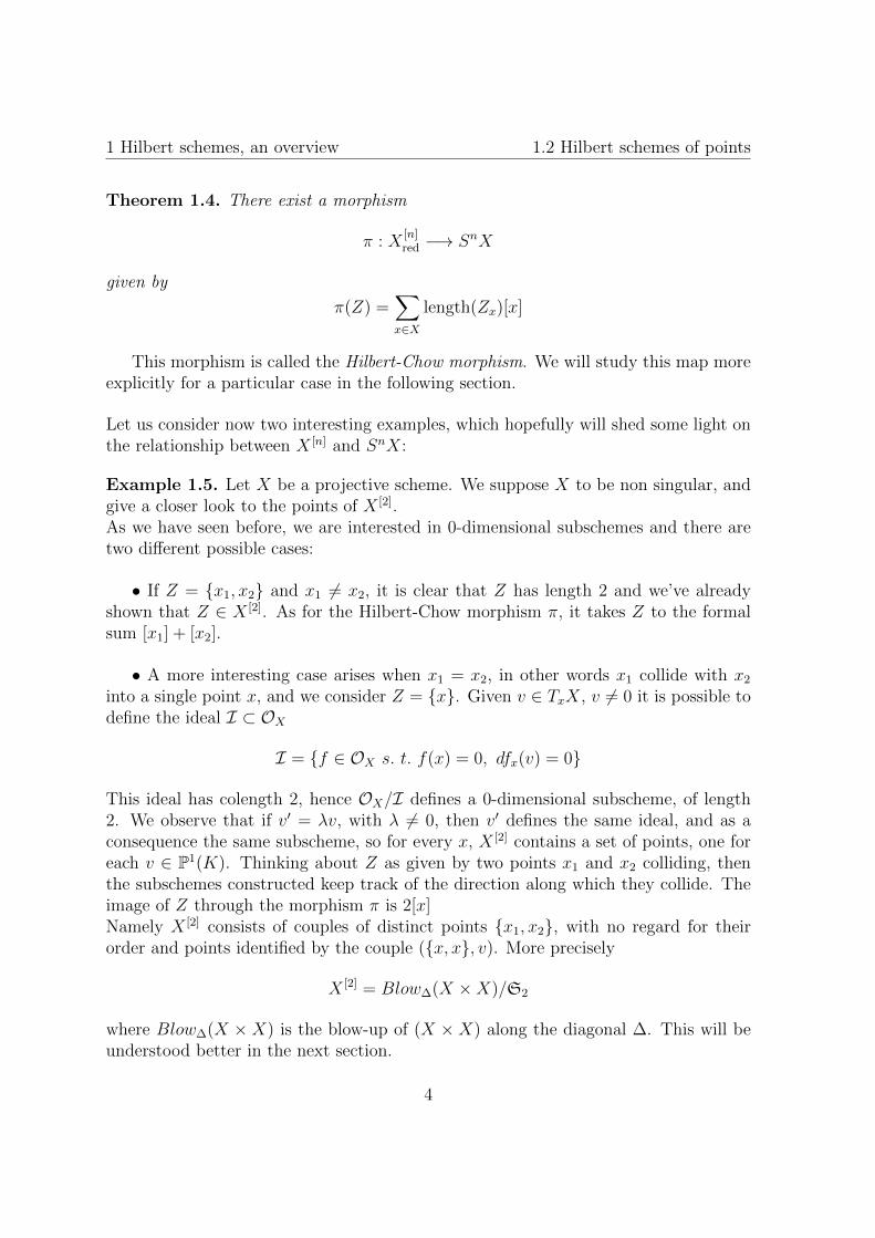
• A more interesting case arises when x1 = x2, in other words x1 collide with x2
into a single point x, and we consider Z = x. Given v ∈ TxX, v 6= 0 it is possible todefine the ideal I ⊂ OX
I = f ∈ OX s. t. f(x) = 0, dfx(v) = 0
This ideal has colength 2, hence OX/I defines a 0-dimensional subscheme, of length2. We observe that if v′ = λv, with λ 6= 0, then v′ defines the same ideal, and as aconsequence the same subscheme, so for every x, X [2] contains a set of points, one foreach v ∈ P1(K). Thinking about Z as given by two points x1 and x2 colliding, thenthe subschemes constructed keep track of the direction along which they collide. Theimage of Z through the morphism π is 2[x]Namely X [2] consists of couples of distinct points x1, x2, with no regard for theirorder and points identified by the couple (x, x, v). More precisely
X [2] = Blow∆(X ×X)/S2
where Blow∆(X ×X) is the blow-up of (X ×X) along the diagonal ∆. This will beunderstood better in the next section.
4
1.2 Hilbert schemes of points 1 Hilbert schemes, an overview
Example 1.6. Let now X = A, the affine line. Then
A[n] = I ⊂ K[z] | I is an ideal, dimK K[z]/I = n =
= f ∈ K[z]|f(z) = zn + an−1zn−1 + . . .+ a0, ai ∈ K = SnA
The equality X [n] = SnX holds more generally if dim X = 1 for X nonsingular,roughly because in this case the tangent space TxX has only one dimension, so thereis no space to choose different directions v.
We conclude the paragraph with a final observation about SnXLet ν = (ν1, . . . , νk) be a partition of n, i.e. a finite sequence of non-increasing positiveintegers such that
∑ki=1 νi = n. For each partition ν of n, we define
SnνX = k∑i=1
νi[xi] ∈ SnX | xi 6= xj, for i 6= j
Then the Snν form a stratification of SnX into locally closed subschemes, and everypoint of SnX lies in a unique Snν . Each Snν has dimension kdim X, where k is thelength of the partition.The Hilbert-Chow morphism implies that the above stratification of SnX induces astratification of X [n], defined by
X [n]ν := π−1(Sn−νX)
For every partition ν = (ν1, . . . , νk) the geometric points of X[n]ν are the union of
subschemes (Z1, . . . , Zk), where Zi is a subscheme of length νi and support xi, thepoints xi being distinct.
1.2.1 Case X = A2
Previously we have described the structure of Hilbert schemes in their generality: fromthis point on we will focus on the simpler case in which dim X = 2. Let’s start witha specific scheme, the affine plane A2. The following result gives an interesting anduseful description of (A2)[n]
Theorem 1.7. Let
H :=
(B1, B2, i)
∣∣∣∣∣∣∣(i) [B1, B2] = 0
(ii) There exists no proper subspace S ( Kn
such that Bα(S) ⊂ S (α = 1, 2) and im i ⊂ S
where Bα ∈ End(Kn) and i ∈ Hom(K,Kn), i.e. i can be identified with a vector in
Kn. Defining the action of GLn(K) on H by
g · (B1, B2, i) = (gB1g−1, gB2g
−1, gi)
5
1 Hilbert schemes, an overview 1.2 Hilbert schemes of points
for g ∈ GLn(K) then the quotient space H := H/GLn(K) is a non singular varietyand represents the functor HilbPX for A2, P = n.
Remark 1.8. Clearly the set of elements (B1, B2, i) such that [B1, B2] = 0 is a Zariskiclosed subset of End(Kn)×End(Kn)×Kn. The second condition, which correspondsto the existence of a cyclic vector i, is a stability condition, and defines an open subsetof it. The quotient is meant in the sense of geometric invariant theory.
Proof. Let us begin with the proof of the isomorphism between H and (A2)[n] as sets.If p ∈ (A2)[n] then we can associate it with the datum (B1, B2, i) = Φ(p) as follows.From the definition, a point p in the Hilbert scheme of points of A2 corresponds toan ideal Ip ⊂ K[z1, z2] s.t. dimK K[z1, z2]/Ip = n: we choose a basis to identifyK[z1, z2]/Ip ' Kn, and we define Bα as the matrix of the multiplication by zα mod Ip,(α = 1, 2)
Bα : K[z1, z2]/Ip −→ K[z1, z2]/Ip
v 7−→ zαv mod I
and i as the element of Kn corresponding to the identity 1 ∈ K[z1, z2]/Ip. B1 andB2 are clearly endomorphisms of K[z1, z2]/Ip, while i is a homomorphism between Kand K[z1, z2]/Ip; moreover multiplications by z1 and z2 commute with each other, so[B1, B2] = 0 and the stability condition holds, indeed:Let S be a subset of K[z1, z2]/Ip, s.t. i(K) ⊂ S and Bα(S) ⊂ S for α = 1, 2, then1 mod (I) ∈ S and zα ∈ S for α = 1, 2. But 1, z1, z2 generate the whole K[z1, z2], so
S cannot be proper. Hence (B1, B2, i) lives in H and the map
Φ : (A2)[n] −→ H
p 7−→ (B1, B2, i)
constructed above, is well defined. Choosing a different basis results precisely in theaction of GLn(K) on the triple (B1, B2, i)
Now, let h = (B1, B2, i) ∈ H. Let ϕh be the morphism ϕh : K[z1, z2] −→ Kn such thatϕh(f) = f(B1, B2)i(1). Then the map
Ψ : H −→ (A2)[n]
h = (B1, B2, i) 7−→ ker ϕh
is well defined:if v ∈ im ϕh ⊂ Kn, then there is a f ∈ K[z1, z2] s.t. v = ϕh(f) = f(B1, B2)i(1),hence Bαv = Bαf(B1, B2)i(1) = f ′(B1, B2)i(1) with f ′ ∈ K[z1, z2], and we have Bαv ∈im ϕh ∀ v ∈ im ϕh and α = 1, 2. Besides im i = i(K) ⊂ im ϕh (it is sufficient totake f as a constant polynomial), so im ϕh is Bα-invariant and contains im i. By the
6
1.2 Hilbert schemes of points 1 Hilbert schemes, an overview
stability condition this implies that ϕh is surjective, and dimK K[z1, z2]/ ker ϕh =n. Finally two data in the same class of the quotient define similar endomorphisms,and as a consequence the kernels of the two morphisms are the same, as well as thecorrespondent points of (A2)[n], thus Ψ can be defined on the quotient space H andthe two maps Φ and Ψ are mutually inverse on H.
The second step consists in proving the non-singularity of H.The differential of the map f : (B1, B2, i) 7−→ [B1, B2] is
d(B1,B2,i)f(E,F, i′) = [E,B2] + [B1, F ]
We recall that, in general, there is a canonical isomorphism between End(Kn, Kn) andEnd(Kn, Kn)∗ given by the non-degenerate canonical bilinear form
Hom(Kn, Kn) 3 A,B 7−→ tr(AB) ∈ K
and that the annihilator of a linear subspace W ∈ V is defined as
W⊥ := ϕ ∈ V ∗ | ϕ(w) = 0 ∀ w ∈ W
Finally, there is an isomorphism between (W ∗)⊥ and V/W . Then we can write thecokernel of df as
coker df = Hom(Kn, Kn)/im df ∼= (im df ∗)⊥
= C ∈ End(Kn) | tr(C([E,B2] + [B1, F ])) = 0 ∀ E,F
Besides we have tr(CEB2 − CB2E + CB1F − CFB1) = tr(EB2C) − tr(ECB2) +tr(FCB1) − tr(FB1C) = tr(E[B2, C]) + tr(F [C,B2]); since this equality has to holdfor all E,F ∈ End(Kn, Kn), we get
coker df = C ∈ End(Kn) | [C,B1] = [C,B2] = 0
Let R be the ring Bk1B
l2i(1)k,l>0. If we consider it as an R-module on itself then the
conditions [C,B1] = [C,B2] = 0 imply that
C : R −→ R
is a morphism of R-modules, since we get
C(v + w) = C(Bk11 B
l12 i(1) +Bk2
1 Bl22 i(1)) = C((Bk1
1 Bl12 +Bk2
1 Bl22 )i(1))
= (Bk11 B
l12 +Bk2
1 Bl22 )C(i(1)) = Bk1
1 Bl12 C(i(1)) +Bk2
1 Bl22 C(i(1))
= C(v) + C(w)
and similarly C(λv) = λC(v) with λ ∈ R. Hence C is determined by the image of i(1),and C(i(1)) can be any vector in Kn, since by the stability condition Bk
1Bl2i(1) span
7

1 Hilbert schemes, an overview 1.2 Hilbert schemes of points
Kn. Therefore there is a bijective correspondence between the endomorphisms whichcommute with B1, B2 and the vectors in Kn, so that the dimensions of the two spacesagree. Thus
dim coker df = dimC ∈ End(Kn) | [C,B1] = [C,B2] = 0 = n
The constant rank of the differential implies that H is non singular, what about thequotient space H?Let us consider the action of GLn(K) on H: if g ∈ GLn(K) stabilizes (B1, B2, i) ∈ Hthen gB1g
−1 = B1, gB2g−1 = B2 and gi = i, so that
i) (g − id)i = 0, i.e. im i ∈ ker (g − id)
ii) if x ∈ker (g − id) then (g − id)(Bαx) = gBαx − Bαx = gBαg−1x − Bαg
−1x =Bαx−Bαg
−1x = Bα(x− g−1x) = 0
Hence ker (g − id) contains im i and is invariant under B1, B2: the stability conditionimplies that g = id, thus the stabilizer of GLn(K)-action is trivial and by Luna’s slice
theorem [11] H = H/GLn(K) has a structure of non singular variety such that the
map H → H is a principal etale fiber bundle for the group GLn(K); since GLn(K)is a special group, then the fact that the principal etale fiber bundle is trivial impliesthat the fiber bundle is locally trivial even in the Zariski topology. Moreover the mapΨ described before provides a flat family of 0-dimensional subschemes H → H.
Finally let us prove the universality of H → H, i.e. if π : Z → U is anotherflat family of 0-dimensional subschemes of A2 of length n, then there exists a uniquemorphism χ : U → H such that the pullback χ∗H → U is Z → U .We observe that if π : Z → U is flat and of length n, then π∗OZ is a OU -moduleand a locally free sheaf of rank n, hence locally it is possible to define B1, B2 as abovefrom multiplication of coordinate functions z1, z2 and i from the constant polynomial1: B1, B2 are commuting OU -linear endomorphisms of π∗OZ and i ∈ Hom(OU , π∗OZ).Fix an open covering Uα of U and trivializations of the restriction of π∗OZ to Uα.
Then (B1, B2, i) defines morphisms Uα → H. If we compose them with the projection
H → H, they glue together to define a morphism φ : U → H: it is precisely themorphism we were looking for because by construction φ∗H is Z. The uniqueness isclear.
Remark 1.9. We point out that according to the proof of the theorem, the ideal Icorresponding to the point h = (B1, B2, i) is given by the kernel of the map ϕh, thus
I = f ∈ K[z1, z2] | f(B1, B2)i(1) = 0
By the stability condition, however, it can be rewritten as
I = f ∈ K[z1, z2] | f(B1, B2) = 0
since ker f(B1, B2) is Bα-invariant and contains im i, hence it cannot be proper.
8
1.2 Hilbert schemes of points 1 Hilbert schemes, an overview
Remark 1.10. Let us fix a point [(B1, B2, i)] in (C2)[n]. Consider the maps
End(Kn, Kn)⊕
GLn(K)ψ−→ End(Kn, Kn)
φ−→ End(Kn, Kn)⊕
Hom(K,Kn)
where ψ is the action ofGLn(K) on the fixed point (B1, B2, i), φ is the map (C1, C2, j) 7→[C1, C2] and their derivatives
Hom(Kn, Kn)⊕
Hom(Kn, Kn)dψ−→ Hom(Kn, Kn)
dφ−→ Hom(Kn, Kn)⊕Kn
(1.1)
Then dψ : G 7→ ([G,B1], [G,B2], Gi) and dφ : (C1, C2, j) 7→ [B1, C2] + [C1, B2], more-over (1.1) is a complex, since
dφ(dψ(G)) = dφ([G,B1], [G,B2], Gi) = [B1, [G,B2]] + [[G,B1], B2] =
= −[B2, [B1, G]]− [G, [B2, B1]] + [[G,B1], B2] =
= ([B1, B2] = 0) = [B2, [G,B1]]− [B2, [G,B1]] = 0
The description of H provided by theorem 1.7 implies that the tangent space of (A2)[n]
at the point (B1, B2, i) is the middle cohomology group of this complex. We havealready seen that the dimension of coker dφ is n, besides if G ∈ ker dψ = G | [G,B1] =[G,B2] = 0, Gi = 0, G 6= 0 then ker G is proper and
i) Gi = 0 ⇒ im i ∈ ker G
ii) given x ∈ ker G then G(Bαx) = Bα(Gx) = 0 ⇒ Bα(ker G) ⊆ ker G
violating the stability condition. Hence dψ is surjective and an easy calculation showsthat the dimension of the tangent space is 2n.
Finally we examine two simple examples:
Example 1.11. First, let us study (A2)[1]. We fix
B1 = λ, B2 = µ λ, µ ∈ K
In this case the group GL1(K) acts as the multiplication on i:the action is (λ, µ, i) 7→ (gλg−1, gµg−1, gi) but g ∈ GL1(K) ∼= K× so that
(gλg−1, gµg−1, gi) = (gg−1λ, gg−1µ, gi) = (λ, µ, gi)
9

1 Hilbert schemes, an overview 1.2 Hilbert schemes of points
Moreover we have seen that i has to be non-zero, so it must be a constant i = k, hence,applying the action of GL1(K) if necessary, we can always assume i = 1.Remark 1.9 shows that the ideal I correspondent to the point (λ, µ, 1) is given by
I = f ∈ K[z1, z2] | f(λ, µ) = 0
This is precisely the ideal of definition of the point (λ, µ) ∈ A2. Thus it it definedthe map (A2)[1] → A2 : (λ, µ, i) 7→ (λ, µ); it is clearly surjective, and it is injective,since if (λ, µ, i) and (λ′, µ′, i′) are mapped into the same point (x, y) then obviouslyx = λ = λ′, y = µ = µ′ and i′ = gi, therefore (λ, µ, i) and (λ′, µ′, i′) coincide in thequotient space H ∼= (A2)[1] and
(A2)[1] ∼= A2
Example 1.12. Now we consider (A2)[2]: the points (B1, B2, i) can be of two differentkinds.(a) Both B1 and B2 have two distinct eigenvalues, therefore they are semisimple andsince they commute , they can be simultaneously diagonalized. Then, rememberinghow GL2(K) acts, we can assume
B1 =
(λ1 00 λ2
)B2 =
(µ1 00 µ2
)i(1) =
(kh
)λ1, λ2, µ1, µ2, k, h ∈ K
with (λ1, µ1) 6= (λ2, µ2).Let us focus on the characteristics of i(1) for these particular matrices: if h = 0 thenS := (x, 0)T , x ∈ K is proper, Bα-invariant and contains im i, since i(η) = ηi(1).Hence by the stability condition we get h 6= 0 and similarly k 6= 0. Moreover, given
g =
(1/k 00 1/h
)then
(gB1g−1, gB2g
−1gi) = (B1, B2, gi), with gi(1) =
(11
)Therefore we can always assume i(1) = (1, 1)T . The corresponding ideal is
I =
f ∈ K[z1, z2] | f(B1, B2)
(11
)= 0
In fact, if f =
n∑i,j=1
aijzi1zj2 then
f(B1, B2) =n∑
i,j=1
aijBi1B
j2 =
n∑i,j=1
aij
(λi1 00 λi2
)(µj1 0
0 µj2
)=
=
(∑ni,j=1 aijλ
i1µ
j1 0
0∑n
i,j=1 aijλi2µ
j2
)=
(f(λ1, µ1) 0
0 f(λ2, µ2)
)10
1.2 Hilbert schemes of points 1 Hilbert schemes, an overview
thus the ideal I is given by
I = f ∈ K[z1, z2] | f(λ1, µ1) = 0 = f(λ2, µ2)
hence
I = I((λ1, µ1)) ∩ I((λ2, µ2)) = I((λ1, µ1), (λ2, µ2))
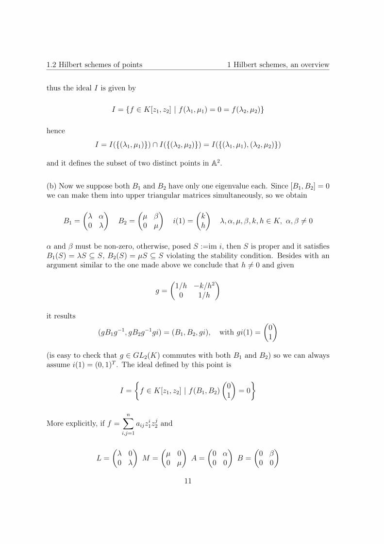
and it defines the subset of two distinct points in A2.
(b) Now we suppose both B1 and B2 have only one eigenvalue each. Since [B1, B2] = 0we can make them into upper triangular matrices simultaneously, so we obtain
B1 =
(λ α0 λ
)B2 =
(µ β0 µ
)i(1) =
(kh
)λ, α, µ, β, k, h ∈ K, α, β 6= 0
α and β must be non-zero, otherwise, posed S :=im i, then S is proper and it satisfiesB1(S) = λS ⊆ S, B2(S) = µS ⊆ S violating the stability condition. Besides with anargument similar to the one made above we conclude that h 6= 0 and given
g =
(1/h −k/h2
0 1/h
)
it results
(gB1g−1, gB2g
−1gi) = (B1, B2, gi), with gi(1) =
(01
)(is easy to check that g ∈ GL2(K) commutes with both B1 and B2) so we can alwaysassume i(1) = (0, 1)T . The ideal defined by this point is
I =
f ∈ K[z1, z2] | f(B1, B2)
(01
)= 0
More explicitly, if f =n∑
i,j=1
aijzi1zj2 and
L =
(λ 00 λ
)M =
(µ 00 µ
)A =
(0 α0 0
)B =
(0 β0 0
)11
1 Hilbert schemes, an overview 1.2 Hilbert schemes of points
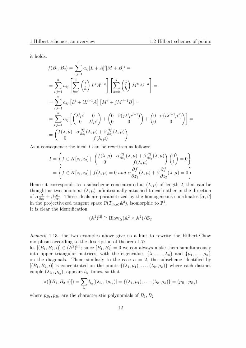
it holds:
f(B1, B2) =n∑
i,j=1
aij[L+ A]i[M +B]j =
=n∑
i,j=1
aij
[i∑
k=0
(ik
)LkAi−k
][j∑
h=0
(jh
)MhAj−h
]=
=n∑
i,j=1
aij[Li + iLi−1A
] [M j + jM j−1B
]=
=n∑
i,j=1
aij
[(λiµj 0
0 λiµj
)+
(0 β(jλiµj−1)0 0
)+
(0 α(iλi−1µj)0 0
)]=
=
(f(λ, µ) α ∂f
∂z1(λ, µ) + β ∂f
∂z2(λ, µ)
0 f(λ, µ)
)As a consequence the ideal I can be rewritten as follows:
I =
f ∈ K[z1, z2] |
(f(λ, µ) α ∂f
∂z1(λ, µ) + β ∂f
∂z2(λ, µ)
0 f(λ, µ)
)(01
)= 0
=
f ∈ K[z1, z2] | f(λ, µ) = 0 and α
∂f
∂z1
(λ, µ) + β∂f
∂z2
(λ, µ) = 0
Hence it corresponds to a subscheme concentrated at (λ, µ) of length 2, that can bethought as two points at (λ, µ) infinitesimally attached to each other in the directionof α ∂
∂z1+ β ∂
∂z2. These ideals are parametrized by the homogeneous coordinates [α, β]
in the projectivezed tangent space P(T(λ,µ)A2), isomorphic to P1.It is clear the identification
(A2)[2] ∼= Blow∆(A2 × A2)/S2
Remark 1.13. the two examples above give us a hint to rewrite the Hilbert-Chowmorphism according to the description of theorem 1.7:let [(B1, B2, i)] ∈ (A2)[n]; since [B1, B2] = 0 we can always make them simultaneouslyinto upper triangular matrices, with the eigenvalues λ1, . . . , λn and µ1, . . . , µnon the diagonals. Then, similarly to the case n = 2, the subscheme identified by[(B1, B2, i)] is concentrated on the points (λ1, µ1), . . . , (λk, µk) where each distinctcouple (λih , µih), appears lih times, so that
π([(B1, B2, i)]) =∑ih
lih [(λih , 1µih)] = (λ1, µ1), . . . , (λk, µk) = (pB1 , pB2)
where pB1 , pB2 are the characteristic polynomials of B1, B2
12
1.3 Further facts and results 1 Hilbert schemes, an overview
Remark 1.14. The non singularity of X [n] holds every time X is non singular and dimX = 2. More precisely:
Theorem 1.15. Suppose X is non singular and dim X = 2 then the following holds.
1. X [n] is non singular and has dimension 2n
2. π : X [n] → SnX is a resolution of singularities.
The proof of (1) comes easily from theorem 1.7:let Z ∈ X [n] and IZ the corresponding ideal. Suppose π(Z) =
∑i νi[xi], where the
points xi are pair wise distinct. Let Z =∐
i Zi the corresponding decomposition. Thenlocally (in the classical topology) X [n] decomposes into a product
∏iX[νi] Thus it is
enough to show that X [n] is non singular at Z when Z is supported at a single point.Hence we may replace X by the affine plane A2.
1.3 Further facts and results
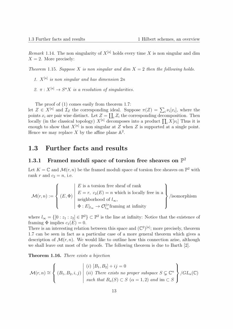
1.3.1 Framed moduli space of torsion free sheaves on P2
Let K = C andM(r, n) be the framed moduli space of torsion free sheaves on P2 withrank r and c2 = n, i.e.
M(r, n) :=
(E,Φ)
∣∣∣∣∣∣∣∣∣E is a torsion free sheaf of rank
E = r, c2(E) = n which is locally free in a
neighborhood of l∞,
Φ : E|l∞ → O⊕rl∞ framing at infinity
/isomorphism
where l∞ = [0 : z1 : z2] ∈ P2 ⊂ P2 is the line at infinity: Notice that the existence offraming Φ implies c1(E) = 0.There is an interesting relation between this space and (C2)[n]; more precisely, theorem1.7 can be seen in fact as a particular case of a more general theorem which gives adescription of M(r, n). We would like to outline how this connection arise, althoughwe shall leave out most of the proofs. The following theorem is due to Barth [2].
Theorem 1.16. There exists a bijection
M(r, n) ∼=
(B1, B2, i, j)
∣∣∣∣∣∣∣(i) [B1, B2] + ij = 0
(ii) There exists no proper subspace S ( Cn
such that Bα(S) ⊂ S (α = 1, 2) and im ⊂ S
/GLn(C)
13
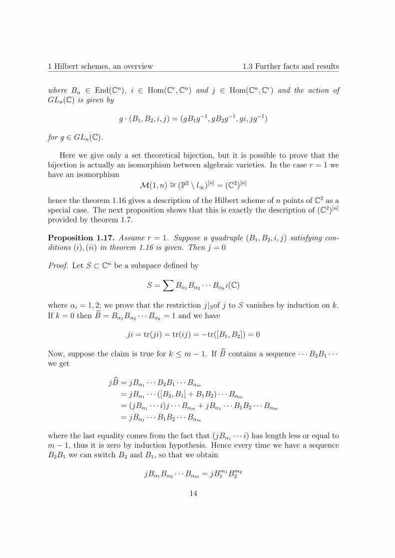
1 Hilbert schemes, an overview 1.3 Further facts and results
where Bα ∈ End(Cn), i ∈ Hom(Cr,Cn) and j ∈ Hom(Cn,Cr) and the action ofGLn(C) is given by
g · (B1, B2, i, j) = (gB1g−1, gB2g
−1, gi, jg−1)
for g ∈ GLn(C).
Here we give only a set theoretical bijection, but it is possible to prove that thebijection is actually an isomorphism between algebraic varieties. In the case r = 1 wehave an isomorphism
M(1, n) ∼= (P2 \ l∞)[n] = (C2)[n]
hence the theorem 1.16 gives a description of the Hilbert scheme of n points of C2 as aspecial case. The next proposition shows that this is exactly the description of (C2)[n]
provided by theorem 1.7.
Proposition 1.17. Assume r = 1. Suppose a quadruple (B1, B2, i, j) satisfying con-ditions (i), (ii) in theorem 1.16 is given. Then j = 0
Proof. Let S ⊂ Cn be a subspace defined by
S =∑
Bα1Bα2 · · ·Bαki(C)
where αi = 1, 2; we prove that the restriction j|Sof j to S vanishes by induction on k.
If k = 0 then B = Bα1Bα2 · · ·Bαk = 1 and we have
ji = tr(ji) = tr(ij) = −tr([B1, B2]) = 0
Now, suppose the claim is true for k ≤ m − 1. If B contains a sequence · · ·B2B1 · · ·we get
jB = jBα1 · · ·B2B1 · · ·Bαm
= jBα1 · · · ([B2, B1] +B1B2) · · ·Bαm
= (jBα1 · · · i)j · · ·Bαm + jBα1 · · ·B1B2 · · ·Bαm
= jBα1 · · ·B1B2 · · ·Bαm
where the last equality comes from the fact that (jBα1 · · · i) has length less or equal tom − 1, thus it is zero by induction hypothesis. Hence every time we have a sequenceB2B1 we can switch B2 and B1, so that we obtain
jBα1Bα2 · · ·Bαm = jBm11 Bm2
2
14
1.3 Further facts and results 1 Hilbert schemes, an overview
with m1 + m2 = m and ms = #l|αl = s, s = 1, 2 and it is sufficient to show the
claim for B = Bm11 Bm2
2 . In this case we have
= jBi = tr(Bij) = −tr(Bm11 Bm2
2 [B1, B2])
= −tr([Bm11 Bm2
2 , B1], B2) = −tr(Bm11 [Bm2
2 , B1]B2)
= −m2−1∑l=0
tr(Bm11 Bl
2[B2, B1]Bm2−l−12 B2)
= −m2−1∑l=0
tr(Bm2−l2 Bm1
1 Bl2[B2, B1])
= −m2−1∑l=0
tr(Bm2−l2 Bm1
1 Bl2ij) = −
m2−1∑l=0
jBm2−l2 Bm1
1 Bl2i
Since jBm2−l2 Bm1
1 Bl2 = jBm1
1 Bm22 we have
jBi = −m2ji
Hence jBi = 0.Since S is Bα-invariant and imi ⊂ S, we must have S = Cn. Therefore j = 0.
The difference between the two descriptions is the appearance of j, which turns outto be 0 when r = 1. We point out that the auxiliary datum j is not actually artificialand it will play an important role when we will construct a hyper-Kahler structure on(C2)[n] in chapter 2.
1.3.2 Symplectic structure
Assume k = C and that X has a holomorphic symplectic form ω, i.e. ω is an elementin H0(X,Ω2
X) which is non degenerate at every point x ∈ X; we wonder if X [n] inheritsthis property. Actually this is true as the following theorem shows
Theorem 1.18. Suppose X has a holomorphic symplectic form ω. Then X [n] has aholomorphic symplectic form.
Before proving it we focus on the particular case X [n] = (C2)[n]; It is possible toprove that the description in theorem 1.7 can be thought as a holomorphic symplecticquotient (actually we will prove that it has a structore of hyper-Kahler quotient),therefore we have a holomorphic symplectic form ω on (C2)[n].As an application of the existence of ω, we give an estimate of the dimension of fibers ofthe Hilbert-Chow map as follows: the parallel traslation of C2 provides the factorization(C2)[n] = C2 × ((C2)[n]/C2). In our description a point in (C2)[n]/C2 corresponds to(B1, B2, i) with tr(B1) =tr(B2) = 0. We have
15
1 Hilbert schemes, an overview 1.3 Further facts and results
Theorem 1.19. The subvariety π−1(n[0]) is isotropic with respect to the holomorphicsymplectic form on (C2)[n]/C2, i.e. the symplectic form restricts to zero on π−1(n[0]).In particular, dim π−1(n[0]) ≤ n − 1. Moreover there exist at least one (n − 1)-dimensional component.
Proof. Let us consider the torus action on C2 given by
φt1,t2 : (z1, z2) 7→ (t1z1, t2z2) for (t1, t2) ∈ C∗ × C∗
This action lifts to (C2)[n] and π−1(n[0]) is preserved under the resulting action. Weobserve that, as t1, t2 goes to infinity, any point in π−1(n[0]) converges to a fixed pointof the torus action: if Z is a non singular point of π−1(n[0]) and v, w are two vectorsin (φt1,t2)∗(v), (φt1,t2)∗(w) converge as t1, t2 → ∞. On the other hand if we considerthe pullback of the symplectic form ω by φt1,t2 we obtain
t1t2ω(v, w) = ω((φt1t2)∗(v), (φt1t2)∗(w))
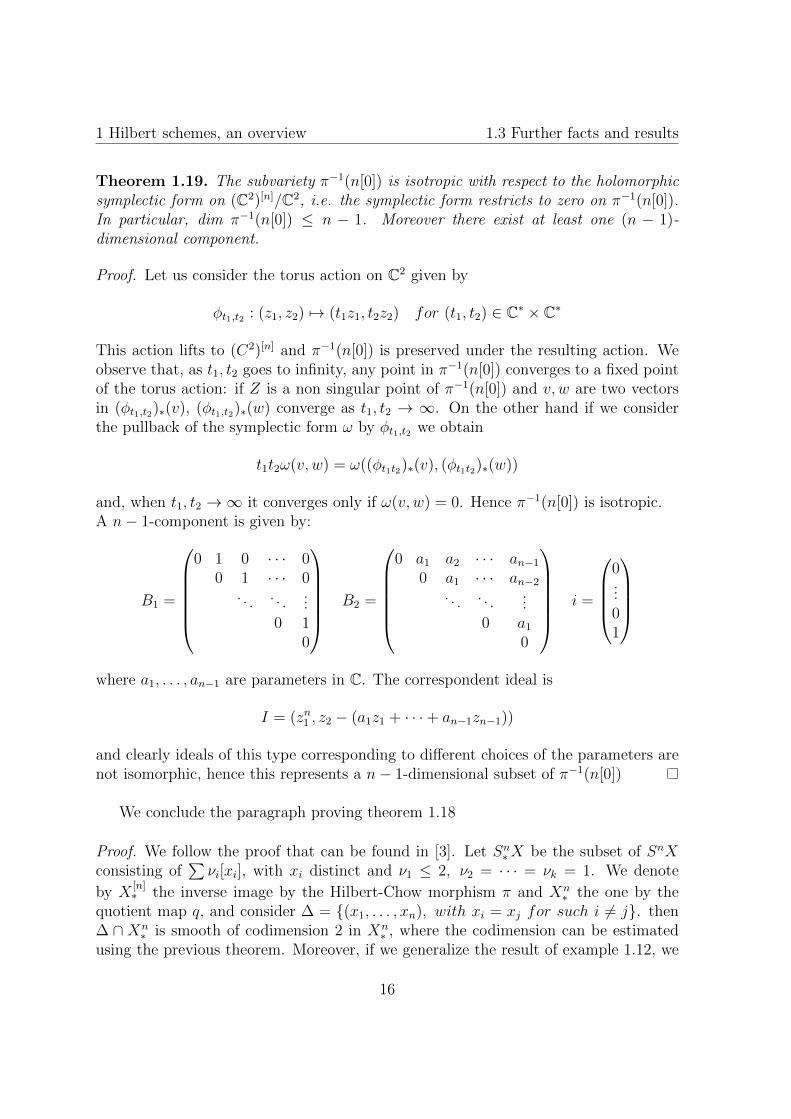
and, when t1, t2 →∞ it converges only if ω(v, w) = 0. Hence π−1(n[0]) is isotropic.A n− 1-component is given by:
B1 =
0 1 0 · · · 0
0 1 · · · 0. . . . . .
...0 1
0
B2 =
0 a1 a2 · · · an−1
0 a1 · · · an−2
. . . . . ....
0 a1
0
i =
0...01
where a1, . . . , an−1 are parameters in C. The correspondent ideal is
I = (zn1 , z2 − (a1z1 + · · ·+ an−1zn−1))
and clearly ideals of this type corresponding to different choices of the parameters arenot isomorphic, hence this represents a n− 1-dimensional subset of π−1(n[0])
We conclude the paragraph proving theorem 1.18
Proof. We follow the proof that can be found in [3]. Let Sn∗X be the subset of SnXconsisting of
∑νi[xi], with xi distinct and ν1 ≤ 2, ν2 = · · · = νk = 1. We denote
by X[n]∗ the inverse image by the Hilbert-Chow morphism π and Xn
∗ the one by thequotient map q, and consider ∆ = (x1, . . . , xn), with xi = xj for such i 6= j. then∆ ∩ Xn
∗ is smooth of codimension 2 in Xn∗ , where the codimension can be estimated
using the previous theorem. Moreover, if we generalize the result of example 1.12, we
16
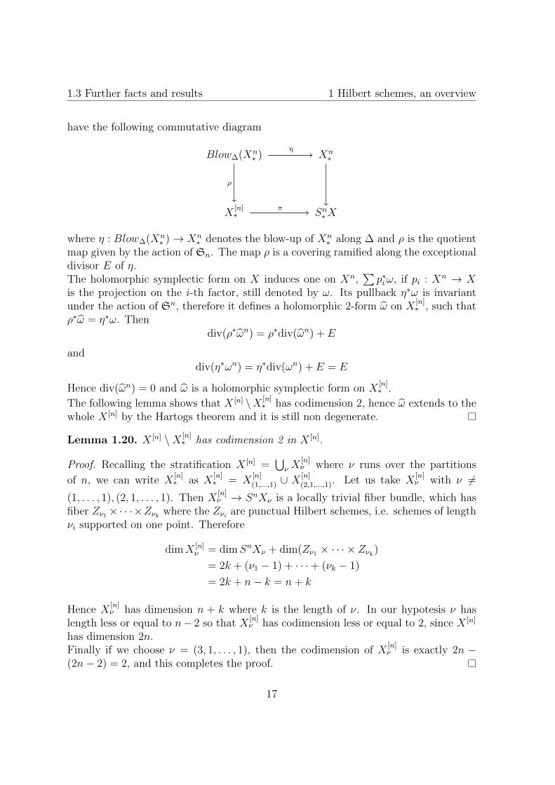
1.3 Further facts and results 1 Hilbert schemes, an overview
have the following commutative diagram
Blow∆(Xn∗ )
η//
ρ
Xn∗
X[n]∗
π // Sn∗X
where η : Blow∆(Xn∗ )→ Xn
∗ denotes the blow-up of Xn∗ along ∆ and ρ is the quotient
map given by the action of Sn. The map ρ is a covering ramified along the exceptionaldivisor E of η.The holomorphic symplectic form on X induces one on Xn,
∑p∗iω, if pi : Xn → X
is the projection on the i-th factor, still denoted by ω. Its pullback η∗ω is invariantunder the action of Sn, therefore it defines a holomorphic 2-form ω on X
[n]∗ , such that
ρ∗ω = η∗ω. Thendiv(ρ∗ωn) = ρ∗div(ωn) + E
anddiv(η∗ωn) = η∗div(ωn) + E = E
Hence div(ωn) = 0 and ω is a holomorphic symplectic form on X[n]∗ .
The following lemma shows that X [n] \X [n]∗ has codimension 2, hence ω extends to the
whole X [n] by the Hartogs theorem and it is still non degenerate.
Lemma 1.20. X [n] \X [n]∗ has codimension 2 in X [n].
Proof. Recalling the stratification X [n] =⋃ν X
[n]ν where ν runs over the partitions
of n, we can write X[n]∗ as X
[n]∗ = X
[n](1,...,1) ∪ X
[n](2,1,...,1). Let us take X
[n]ν with ν 6=
(1, . . . , 1), (2, 1, . . . , 1). Then X[n]ν → SnXν is a locally trivial fiber bundle, which has
fiber Zν1×· · ·×Zνk where the Zνi are punctual Hilbert schemes, i.e. schemes of lengthνi supported on one point. Therefore
dimX [n]ν = dimSnXν + dim(Zν1 × · · · × Zνk)
= 2k + (ν1 − 1) + · · ·+ (νk − 1)
= 2k + n− k = n+ k
Hence X[n]ν has dimension n + k where k is the length of ν. In our hypotesis ν has
length less or equal to n− 2 so that X[n]ν has codimension less or equal to 2, since X [n]
has dimension 2n.Finally if we choose ν = (3, 1, . . . , 1), then the codimension of X
[n]ν is exactly 2n −
(2n− 2) = 2, and this completes the proof.
17
1 Hilbert schemes, an overview 1.3 Further facts and results
1.3.3 The Douady space
We always assumed X to be projective, but Hilbert schemes can be generalized to thecase X is a complex analytic space: the objects arising are called Douady spaces. Welimit ourself to consider the zero-dimensional case, and denote them still by X [n]. Wewould like to observe that many of the results in this first chapter can be generalizedto Douady spaces, for instance:
• X [n] is a complex space;
• the Hilbert-Chow morphism π : X [n] → SnX is still defined and it is a holomor-phic function;
• theorem 1.15 is still true in the complex analytic case (the proof still works);
• finally X [n] has a Kahler metric if X is compact and has a Kahler metric.
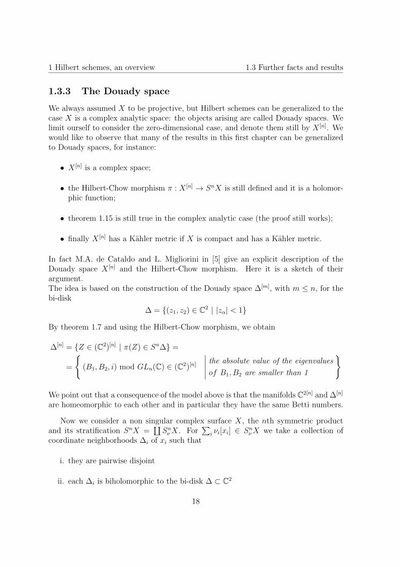
In fact M.A. de Cataldo and L. Migliorini in [5] give an explicit description of theDouady space X [n] and the Hilbert-Chow morphism. Here it is a sketch of theirargument.The idea is based on the construction of the Douady space ∆[m], with m ≤ n, for thebi-disk
∆ = (z1, z2) ∈ C2 | |zα| < 1
By theorem 1.7 and using the Hilbert-Chow morphism, we obtain
∆[n] = Z ∈ (C2)[n] | π(Z) ∈ Sn∆ =
=
(B1, B2, i) mod GLn(C) ∈ (C2)[n]
∣∣∣∣∣ the absolute value of the eigenvalues
of B1, B2 are smaller than 1
We point out that a consequence of the model above is that the manifolds C2[n] and ∆[n]
are homeomorphic to each other and in particular they have the same Betti numbers.
Now we consider a non singular complex surface X, the nth symmetric productand its stratification SnX =
∐SnνX. For
∑i νi[xi] ∈ SnνX we take a collection of
coordinate neighborhoods ∆i of xi such that
i. they are pairwise disjoint
ii. each ∆i is biholomorphic to the bi-disk ∆ ⊂ C2
18
1.3 Further facts and results 1 Hilbert schemes, an overview
If we consider the complex manifold∏
i(∆i)[νi] then we have a set of charts which glue
by the universal property of the Douady space for ∆ and get a complex manifold X [n]:it follows by the construction that X [n] carries a universal family Z → X [n] and thusit represents the functor HilbPX for P = n. The local (Douady-Barlet)
∏i(∆i)
[νi] →∏i S
νi(∆i) also glue, defining a global map π : X [n] → SnX (the analogous of theHilbert-Chow morphism in the algebraic case).
19

Chapter 2
Hyper-Kahler metric on (C2)[n]
The aim of the chapter is to construct an Hyper-Kahler metric on (C2)[n], identifyingit with an Hyper-Kahler quotient. We will use the description provided by theorem1.16.Let us start with a brief introduction to geometric invariant theory quotients in theaffine case.
2.1 Geometric invariant theory quotients
Let G be a reductive algebraic group and let X be an affine variety, i.e. there existsn > 0 such that X ⊂ An as a closed subset. Equivalently, X can be recovered form itscoordinate ring. With a slight abuse we will write X = Spec R. We assume that Gacts linearly on An and hence on X. We would like to consider the quotient space ofX under the action of G, but the set theoretical quotient X/G usually behaves badlyand it is not even Hausdorff in general. This is due to the fact that G is only rarelycompact, hence the orbits of its action may not be closed and contain orbits of smallerdimension in their closures. In order to clarify what can happen, we begin with asimple example.
Example 2.1. Consider the action of C× on C2 given by matrices(λ 00 λ−1
)∈ SL2(C), λ ∈ C×
Hence the action takes (z1, z2) to (λz1, λ−1z2) and the orbits are:
• the hyperbola hα = (x, y) | xy = α for α 6= 0• the punctured x-axis (x, y) | y = 0, x 6= 0• the punctured y-axis (x, y) | y 6= 0, x = 0• the origin.
21

2 Hyper-Kahler metric on (C2)[n] 2.1 Geometric invariant theory quotients
We observe that the orbits hα are closed and in bijection with C×. The puncturedaxes instead are not closed and their closures intersect in the origin, which is anorbit of smaller dimension, therefore if we consider the set theoretic quotient theseorbits correspond to points that cannot be separated, making the quotient space nonHausdorff: the idea of the geometric invariant theory is to identify the three orbitswith each other in an equivalence class.
Let us construct the quotient in the affine case: given the affine variety X = Spec R,the action of G on X induces a G-action on R. Let RG be the ring of invariants. Atheorem of Nagata ensures that this is a finitely generated algebra. We define
X//G = Spec(RG)
This is called the affine geometric invariant theory quotient of X by G. The principalresult of geometric invariant theory states that
Theorem 2.2 ([15],[13]). There exists a surjective morphism
φ : X −→ X//G
induced by the inclusion RG ⊂ R. Moreover φ(x) = φ(y) if and only if
G · x ∩G · y 6= ∅ (2.1)
The underlying space of X//G is the set of closed G-orbits modulo the equivalencerelation defined by x ∼ y if and only if 2.1 holds.
Retrieving the example we have made before we get:
C2 = Spec C[x, y]
andC[x, y]G = C[xy]
since λxλ−1y = xy, hence
C2//C× = Spec C[xy] ∼= C
It is possible to consider even a slightly different construction; the idea is to mimicthe construction used in the projective case for an affine variety. Namely we considerthe action of G on X and, after choosing a character of G, we lift it to the trivialfiber bundle X × C, using it to obtain a graded algebra. More formally we choose acharacter χ : G→ C∗, then the lifting of the action is defined by
g · (x, z) = (g · x, χ(g)−1z) for (x, z) ∈ X × C
22
2.1 Geometric invariant theory quotients 2 Hyper-Kahler metric on (C2)[n]
If X = Spec R, then let RG,χn be the space of functions satisfying
f(g · x) = χ(g)nf(x)
It can be identified with the space of G invariant functions on X×C. Hence the directsum
⊕n≥0R
G,χn is a finitely generated graded algebra. Therefore we can define
X//χG := Proj
(⊕n≥0
RG,χn
)We still call it the geometric invariant theory quotient of X.
In geometric language V//χG can be described as follows. We say that x ∈ X isχ-semistable if there exists f ∈ RG,χn with n ≥ 0 such that f(x) 6= 0. This happensif and only if the closure of G · (x, z) does not intersect with X × 0 for z 6= 0. LetXss(χ) be the set of χ semistable points. We introduce an equivalence relation ∼ onV ss(χ) by defining x ∼ y if and only if G · x∩G · y is non empty in Xss(χ). It is alwayspossible to take a representative x so that G · (x, z) is closed for z 6= 0 and G · x isclosed in Xss(χ) for such a representative x. Therefore the quotient space Xss(χ)/ ∼is bijective to the set of orbits G ·x such that G · (x, z) is closed for z 6= 0. Then X//χGis Xss(χ)/ ∼.
Finally we observe that RG,χ0is the ring of the invariants on X, hence the inclusion
RG = RG,χ0 ⊂ RG,χn induces a morphism
π : X//χG −→ X//G (2.2)
2.1.1 Geometric invariant theory and the moment map
Let V be a vector space over C with an hermitian metric, G be a connected closed Liesubgroup of U(V ) and GC its complexification; the Lie algebra of G is denoted by g.We point out that since G is compact then its complexification is a reductive group,hence it is possible to apply in this particular case the second construction made inthe previous paragraph.Let χ : G→ U(1) be a character and let χ also denotes its complexification χ : GC →C∗. Consider the trivial line bundle V × C over V . We use χ to construct the GITquotient V//χG
C and we define the map µ : V → g∗ by
〈µ(x), ξ〉 =1
2(√−1ξx, x) for x ∈ V, ξ ∈ g
It is a special case of the moment map, which is defined for an action on a symplecticmanifold (we will use it again in the following chapter). Now we consider the function
p(x,z)(g) = logN(g · (x, z)) for z 6= 0
where N(x, z) = |z|e 12||x||2 . This map has the following properties
23
2 Hyper-Kahler metric on (C2)[n] 2.1 Geometric invariant theory quotients
Proposition 2.3. For z 6= 0, the map p(x,z) has the following properties
1. p(x,z) descends to a function on G \ GC/GC(x,z), where GC
(x,z) is the stabilizer of
(x, z).
2. p(x,z) is a convex function on G \GC.
3. g is a critical point if and only if 〈µ(g · x), ξ〉 =√−1dχ(ξ).
4. All critical points are minima of p(x,z).
5. If p(x,z) attains its minimum, it does so on exactly one double coset G \ g/GC(x,z)
6. p(x,z) attains minimum if and only if GC · (x, z) is closed in V × C.
Proof. For ξ ∈ g it holds:
i.d
dtp(x,z)(exp t
√−1ξg) = 〈µ(exp t
√−1ξgx), ξ〉 − dχ(
√−1ξ)
ii.d2
dt2p(x,z)(exp t
√−1ξg) = 2||ξ exp t
√−1ξgx||2
Assertion 2. comes from ii., since 2||ξ exp t√−1ξgx||2 ≥ 0; assertion 3. instead comes
from i. and the fact that ξ is generic, because g is critical if and only if (i.) = 0 fort = 0; this is equal to require that 〈µ(gx), ξ〉 − dχ(
√−1ξ) = 0, hence the assertion.
The fourth statement is true since p(x,z) is convex and any two points in G \ GC canbe joined by a geodesic.To prove assertion 5. suppose p(x,z) attains minimum at g and exp
√−1ξ · g. Then the
convexity impliesp(x,z)(exp t
√−1ξg) = const
Therefore we get ξgx = 0 by setting t = 0 in ii.. Hence we have exp√−1ξgx = gx, i.e.
g−1 exp√−1ξg ∈ GC
x . Now we prove assertion 6. Suppose GC · (x, z) is closed. SinceGC · (x, z) and V × 0 are mutually disjoint, closed subsets, there exists an invariantpolynomial P = zP1(x) + · · ·+ znPn(x) which satisfies
P ≡
1 on GC · (x, z)0 on V × 0
Suppose N(x, z) = |z|e 12||x||2 ≤ C. Then |z| is bounded. Moreover
1 = |zP1(x) + · · ·+ znPn(x)|≤ C|P1(x)|e−
12||x||2 + · · ·+ Cn|P1(x)|e−
n2||x||2 ≤ C ′e−
14||x||2
24

2.1 Geometric invariant theory quotients 2 Hyper-Kahler metric on (C2)[n]
Thus ||x|| is bounded. Therefore p(x,z) attains a minimum. Conversely suppose p(x,z)
attains a minimum. We may assume it does so at g = e, replacing x if necessary. Letg⊥x be the orthogonal complement of gx in g. By ii. we have
d2
dt2p(x,z)(exp t
√−1ξ) > 0
for any 0 6= ξ ∈ g⊥x . Hence we can choose a positive constant ε so that
d2
dt2p(x,z)(exp t
√−1ξ) ≥ ε
for ξ ∈ g⊥x with ||ξ|| = 1 and t ∈ [0, 1]. Therefore we have
d2
dt2p(x,z)(exp t
√−1ξ) ≥ ε
for ξ ∈ g⊥x with ||ξ|| = 1 and t = 1. The same inequality holds for t ≥ 1 since p(x,z) isconvex. It implies
p(x,z)(exp t√−1ξ) ≥ ε(t− 1) + p(x,z)(exp
√−1ξ) for t ≥
Thus p(x,z)(exp t√−1ξ) diverges as t→∞. This implies the orbit GC · x is closed.
Corollary 2.4. There exists a bijection between µ−1(√−1dχ)/G and the set x ∈
V | GC · (x, z) is closed for z 6= 0
Proof. If x ∈ µ−1(0)/G then GC · (x, z) is closed for z 6= 0 by assertions 3., 4., 6.of proposition 2.3 : x ∈ µ−1(0)/G implies that p(x,z) attains its minimum and thishappens if and only if GC · (x, z) is closed. Hence it is well posed the map
µ−1(√−1dχ)/G −→ x ∈ V | GC · (x, z) is closed for z 6= 0
The surjectivity of the map follows from 3. and 6. while injectivity comes from 5.
2.1.2 Description of (C2)[n] as a GIT quotient
Looking at theorem 1.16 we consider Hermitian vector spaces V and W whose di-mensions are n and 1 respectively. Then M = End(V, V )⊕End(V, V )⊕Hom(W,V )⊕Hom(V,W ) becomes a vector space with an Hermitian product. We consider the actionof U(V ) given by
(B1, B2, i, j) 7−→ (g−1B1g, g−1B2g, g
−1i, jg) (2.3)
25
2 Hyper-Kahler metric on (C2)[n] 2.1 Geometric invariant theory quotients
The correspondent moment map µ1 : V → u(V )∗ is defined by
µ1(B1, B2, i, j) =
√−1
2([B1, B
†1] + [B2, B
†2] + ii† − j†j)
We introduce a map µC given by
µC(B1, B2, i) = [B1, B2] + ij
Then this is a holomorphic function from M to gl(V ) and µC is GL(V ) invariant.Finally we define χ by
χ(g) = (detg)l
where l is an arbitrary positive integer. Then the following theorem holds
Theorem 2.5.
(C2)[n] = µ−1C (0)//χGLn(C) ∼= µ−1
1 (√−1dχ) ∩ µ−1
C (0)/U(n)
Proof. The second equality comes from corollary 2.4. Besides (B1, B2, i, j) ∈ µ−1C (0)
belongs to H (where H is the one defined in theorem 1.7) if and only if j = 0 and thestability condition in theorem 1.16 holds. Hence the only thing we need to prove is thenext lemma.
Lemma 2.6. (B1, B2, i, j) satisfy the stability condition in theorem 1.16 if and only ifGC · (x, z) is closed for z 6= 0
Proof. Suppose GC · (x, z) is closed for z 6= 0. And suppose there exists a subspace Swhich satisfies the followingi. S is Bα-invariant (α = 1, 2)ii. im i ⊂ S.Taking a complementary subspace S⊥ we decompose V as S ⊕ S⊥. Then we have
Bα =
(∗ ∗0 ∗
)i =
(∗0
)
If we consider g(t) =
(1 00 t−1
), then we have
g(t)Bαg(t)−1 =
(∗ t∗0 ∗
)g(t)i = i
On the other hand we have (detg)−lz = tl dimS⊥z → 0 as t → 0, but this contradictsthe closedness of GC · (x, z).
26
2.2 Hyper-Kahler quotients 2 Hyper-Kahler metric on (C2)[n]
Now we suppose the stability condition is satisfied. If GC · (x, z) is not closed, thenby the Hilbert criterion Theorem (Birkes [4]), there exists a map λ : C∗ → GL(V )which satisfies the condition: limt→ λ(t) · (x, z) exists and this limit is contained withinGC \GC · (x, z). Let us take weight decomposition of V with respect to λ
V =⊕m
V (m)
with V (m) = v ∈ V | λ(t) · v = tmv. The existence of limit implies
Bα(V (m)) ⊆⊕l≥m
V (l) im i ⊂⊕m≥0
V (m)
Hence by the stability condition we have⊕m≥0
V (m)
Therefore detλ(t) = tN for some N ≥ 0.If N = 0 then V = V (0), so that λ ≡ 1 and λ(t) · (x, z) = (x, z), but this is impossiblebecause limt→0 /∈ GC · (x, z).Otherwise, if N > 0 then
λ(t) · (x, z) = (λ(t)xλ(t)−1, (detλ(t))−lz) = (λ(t)xλ(t)−1, t−lNz)
diverges as t→ 0. Hence the contradiction.
Remark 2.7. The morphism 2.2 in this specific case can be rewritten as
π : µ−1C (0)//χGLn(C) −→ µ−1
C (0)//GLn(C)
and it is possible to prove ([14]) that µ−1C (0)//GLn(C) is (isomorphic to?) SnC2, hence
we recover the Hilbert-Chow morphism.
2.2 Hyper-Kahler quotients
This section is devoted to show that the quotient in theorem 2.5 is in fact a hyper-Kahler quotient. Let us begin with a brief review on the Kahler and hyper-Kahlerstructures.
Definition 2.8. Let X be a 2n-dimensional manifold. A Kahler structure of X is apair given by a Riemannian metric g and by an almost complex structure I, whichsatisfies the following conditions:
27
2 Hyper-Kahler metric on (C2)[n] 2.2 Hyper-Kahler quotients
1. g is hermitian for I, i.e. g(Iv, Iw) = g(v, w) for v, w ∈ TX
2. I is integrable
3. If we define a 2-form ω by
ω(v, w) = g(Iv, w) for v, w ∈ TX
then dω = 0.
The 2-form ω is called the Kahler form associated with (g, I).
It is known (see e.g. [10]) that the above conditions are equivalent to requiring thatI is parallel with respect to the Levi-Civita connection of g, i.e. ∇I = 0. This is alsoequivalent to the condition
(the holonomy group of ∇) ⊆ U(n)
The hyper-Kahler structure is a quaternionic version of the Kahler structure, with thedifference that there is no good definition of integrability for the almost hyper-Kahlerstructure. Hence the definition is given generalizing the equivalent definition we havejust discuss.
Definition 2.9. Let X be 4n-dimensional manifold. A hyper-Kahler structure of Xconsists of a Riemannian metric g and a triple of almost complex structures I, J , Kwhich satisfy the following conditions:
1. g(Iv, Iw) = g(Jv, Jw) = g(Kv,Kw) = g(v, w) for v, w ∈ TX
2. (I, J,K) satisfies I2 = J2 = K2 = IJK = −1
3. (I, J,K) are parallel with respect to the Levi-Civita connection of g, i.e. ∇I =∇J = ∇K = 0
The above conditions are equivalent to the condition
(the holonomy group of ∇) ⊆ Sp(n)
.
Remark 2.10. Each one of (g, I), (g, J), (g,K) defines a Kahler structure, and it isalways possible to construct a holomorphic symplectic form: let us pick up I andcombine the other Kahler forms as ωC = ω2 +
√−1ω3. Then
ωC(Iv, w) = g(JIv, w) +√−1g(KIv, w) =
=√−1(g(Jv, w) +
√−1g(Kv,w)) =
√−1ωC(v, w)
This means that ωC is of type (2,0). Moreover it is clear that dωC = 0 and ωC is notdegenerate. Then ωC is a holomorphic symplectic form.
28
2.2 Hyper-Kahler quotients 2 Hyper-Kahler metric on (C2)[n]
Hyper-Kahler structures are not easy to construct or flexible: the following quo-tient, which was introduced by Hitchin et al.[9] as an analogue of Marsden-Weinsteinquotients for symplectic manifolds is a powerful way to construct new hyper-Kahlermanifolds.
Let (X, g, I, J,K) be a hyper-Kahler manifold, and ω1, ω2, ω3 the Kahler forms cor-responding to I, J,K. Suppose that a compact Lie group G acts on X preservingg, I, J,K.
Definition 2.11. A map
µ = (µ1, µ2, µ3) : X → R3 × g∗
is said to be a hyper-Kahler moment map if we have the following:
1. µ is G-equivariant, i.e. µ(g·) = Ad∗g−1µ(x)
2. 〈dµ(v), ξ〉 = ωi(ξ∗, v) for any v ∈ TX, any ξ ∈ g and i = 1, 2, 3, where ξ∗ is a
vector field generated by ξ
We take ζ = (ζ1, ζ2, ζ3) ∈ R3 ⊗ g∗ which satisfies Ad∗g(ζi) = ζi for any g ∈ G,(i = 1, 2, 3). Then µ−1(ζ) is invariant under the G-action. So we can consider thequotient space µ−1(ζ)/G.
Theorem 2.12. Suppose G-action on µ−1(ζ) is free. Then the quotient space µ−1(ζ)/Gis a smooth manifold and has a Riemannian metric and a hyper-Kahler structure in-duced from those on X.
This quotient space is called a hyper-Kahler quotient.
Remark 2.13. Let i be the natural inclusion µ−1(ζ) → X and π the natural pro-jection µ−1(ζ) → µ−1(ζ)/G. Let ω1, ω2, ω3 be the Kahler forms associated with thehyper-Kahler structure on X and ω′1, ω
′2, ω
′3 the forms associated with the hyper-Kahler
structure on µ−1(ζ)/G. Then we say that the hyper-Kahler structure on µ−1(ζ)/G isinduced by that on X if π∗ω′α = i∗ωα, with α = 1, 2, 3.
Remark 2.14. Take x ∈ µ−1(ζ) and consider the differential
dµx : TxX −→ R3 ⊗ g∗
If the G-action is free on µ−1(ζ) the tangent space of the orbit through x, denoted byVx is isomorphic to g under the identification
ξ 7−→ ξ∗x ∈ Vx, ξ ∈ g
Before proving the theorem, we give proof of the following lemmas.
29
2 Hyper-Kahler metric on (C2)[n] 2.2 Hyper-Kahler quotients
Lemma 2.15. Vx, IVx, JVx, KVx are orthogonal to each other.
Proof. Let ξ, η ∈ g. Since µi is equivariant, we have µ(exp(tη)x) = ζ for any t ∈ R.Differentiating with respect to t we have
dµx(η∗x) = 0
hence we haveg(Iξ∗x, η
∗x) = ω1(ξ∗x, η
∗x) = 〈dµi,x(η∗x), ξ〉 = 0
Thus Vx is orthogonal to IVx; the same argument proves that it is orthogonal to JVxand KVx. Moreover I, J,K are hermitian, hence
g(Iξ∗x, Jη∗x) = g(I2ξ∗x, IJη
∗x) = −g(ξ∗x, Kη
∗x) = 0
g(Iξ∗x, Kη∗x) = g(ξ∗x, Jη
∗x) = 0
g(Jξ∗x, Kη∗x) = −g(ξ∗x, Iη
∗x) = 0
This completes the proof.
Lemma 2.16. Let (X, g) a Riemannian manifold with skew adjoint endomorphismsI, J,K of the tangent bundle TX satisfying conditions 1.,2. of definition 2.9. Then(g, I, J,K) is hyper-Kahler if and only if the associated Kahler forms ω1, ω2, ω3 areclosed.
Proof. If (g, I, J) is hyper-Kahler, then clearly ω1, ω2, ω3 are closed, since (g, I), (g, J),(g,K) are Kahler structures. Hence we need to show only the converse: we shall provethe integrability of I using the Newlander-Niremberg theorem. Let v, w be complex-valued vector fields, then
ω2(v, w) = g(Jv, w) = g(KIv, w) = ω3(Iv, w)
Hence v is of type (1,0) with respect to I, i.e. Iv =√−1v if and only if
ivωC = 0 (2.4)
where ωC = ω2 −√−1ω3.
Now we choose v, w of type (1,0) with respect to I and denote by Lv the Lie derivativewith respect to the vector field v. Then we have
i[v,w]ωC
=LviwωC − iwLvωC by the naturality of the Lie derivative
=− iwd(ivωC) by 2.4 for w and the closedness of ωC
=0 by 2.4 for v
Therefore [v, w] is of type (1,0). The Newlander-Niremberg theorem implies that I isintegrable and the same argument shows that the same holds for J,K.
30

2.2 Hyper-Kahler quotients 2 Hyper-Kahler metric on (C2)[n]
Proof of theorem 2.12. Let ξ be in g, and consider a tangent vector Iξ∗x ∈ TxX. Thenwe have
d〈µx(Iξ∗x), η〉 = (ω1(η∗x, Iξ∗x), ω2(η∗x, Iξ
∗x), ω3(η∗x, Iξ
∗x))
= (g(Iη∗x, Iξ∗x), g(Jη∗x, Iξ
∗x), g(Kη∗x, Iξ
∗x))
= (g(η∗x, ξ∗x), 0, 0)
where the last equality comes from lemma 2.15. Similarly we get
d〈µx(Jξ∗x), η〉 = (0, g(η∗x, ξ∗x), 0)
d〈µx(Kξ∗x), η〉 = (0, 0, g(η∗x, ξ∗x))
Hence dµx is surjective, which implies that ζ is a regular value and µ−1(ζ) is a sub-manifold of X whose tangent space is kerdµx. On the other hand it holds
d〈µx(v), η〉 = (ω1(η∗x, v), ω2(η∗x, v), ω3(η∗x, v))
= (g(Iη∗x, v), g(Jη∗x, v), g(Kη∗x, v))
therefore the kernel of dµx is the orthogonal complement of IVx ⊕ JVx ⊕KVx.Since the G-action on µ−1(ζ) is free, the slice theorem implies that the quotient spaceµ−1(ζ)/G has a structure of a C∞-manifold such that the tangent space TG·xµ
−1(ζ)/Gat the orbit G · x is isomorphic to the orthogonal complement of Vx in Txµ
−1(ζ). Thusthe tangent space is the orthogonal complement of Vx ⊕ IVx ⊕ JVx ⊕ KVx in TxX,which is invariant under I, J,K, hence the induced almost complex structure. Therestriction on the Riemannian metric g induces a Riemannian metric on the quotientµ−1(ζ)/G. In order to show that these define a hyper-Kahler structure, it is enough tocheck that the associated Kahler forms ω1, ω2, ω3 are closed by lemma 2.16.Let i : µ−1(ζ) → X be the inclusion and π : µ−1(ζ)→ µ−1(ζ)/G the projection.By definition, it holds i∗ωi = π∗ω′i for i = 1, 2, 3. Therefore
π∗(dω′i) = d(π∗ω′i) = d(i∗ωi) = i∗(dωi) = 0
But π is a submersion, hence π∗(dω′i) = 0 implies dω′i = 0
Let us apply this construction to the description in theorem 2.5: let M be as insection 2.1.1, then the antilinear endomorphism
J(B1, B2, i, j) = (B†2,−B†1, j†,−i†)
makes M into a quaternion vector space (J2 = −Id). Hence M is a (flat) hyper-Kahler manifold and the action 2.3 of U(V ) preserves the hyper-Kahler structure. Ifwe consider the maps
µ1(B1, B2, i, j) =
√−1
2([B1, B
†1] + [B2, B
†2] + ii† − j†j)
31
2 Hyper-Kahler metric on (C2)[n] 2.2 Hyper-Kahler quotients
µC(B1, B2, i) = [B1, B2] + ij
and decompose the latter asµC = µ2 +
√−1µ3
considering gln(C) as the complexification of u(V ), then the map
µ = (µ1, µ2, µ3) : M −→ R3 ⊗ u(V )
is a hyper-Kahler moment map and the action of U(V ) on µ−1(√−1dχ, 0, 0) is free.
Thus by theorem 2.12 we have
Corollary 2.17. µ−11 (√−1dχ) ∩ µ−1
2 (0) ∩ µ−13 (0)/U(V ) = (C2)[n] is a hyper-Kahler
quotient. In particular, (C2)[n] has a hyper-Kahler structure.
Remark 2.18. Let us take√−1ζidV ∈ R3⊗u(V ) for any ζ ∈ R3. Then the U(V )-action
is free on µ−1(√−1ζidV ) if ζ 6= 0 and we get essentially the same hyper-Kahler mani-
folds. More precisely there exists a map from µ−1(√−1ζidV )/U(V ) to µ−1
1 (√−1|ζ|idV )
which is an isometry and transforms the hyper-Kahler structure (I, J,K) into I ′
J ′
K ′
= R
IJK
for some R ∈ SO(3) satisfying (|ζ|, 0, 0)T = Rζ.We observe that µ−1(
√−1ζidV )/U(V ) is not isomorphic to (C2)[n] as a complex mani-
fold in general. Let us decompose ζ = (ζR, ζC) by choosing an identification R3 ∼= R⊕C.We decompose the hyper-Kahler moment map into (µR, µC). If ζC 6= 0 it is possible toprove that
i. µ−1C (ζ) is non singular
ii. every GL(V )-orbit in µ−1C (ζ) is closed
iii. the stabilizer of any point in µ−1C (ζ)/U(V ) = µ−1
C (ζ)/GL(V ) is trivial
In particular we have µ−1(ζ)/U(V ) = µ−1C (ζ)/GL(V ). The right hand side is an affine
algebro geometric quotient and in particular it is an affine algebraic variety. As acorollary we have
Theorem 2.19. (C2)[n] is diffeomorphic to an affine algebraic manifold.
32
Chapter 3
The Poincare polynomial of (C2)[n]
In this chapter we shall calculate the Poincare polynomial of (C2)[n]: given a manifoldX, its general definition is the following
Pt(X) :=∑n≥0
tndimHn(X)
where H∗() is the cohomology group with rational coefficients. We will use theBialynicki-Birula decomposition associated with the torus action on (C2)[n] and com-pute the Poincare polynomial using Morse theory. Thus, as a first step, we need toprove that the Morse function arising from the moment map connected to the torusaction is perfect. In fact we will prove the statement for a generic compact symplecticmanifold (considering the case in which the critical submanifolds are points) and thenuse it for our specific case.
3.1 Perfectness of the Morse function
Let (X,ω) be a compact symplectic manifold and T a compact torus. We suppose thatthere exist a T -action on X preserving the 2-form ω: it is defined the pairing
〈, 〉 : t∗ × t −→ R
where t is the Lie algebra of T ; besides any ξ in t induces a vector field ξ∗ on Xdescribing the infinitesimal action of ξ. The corresponding moment map for the T -action on X is the map
µ : X −→ t∗
satisfying
d 〈µ, ξ〉 = iξ∗ω for ξ ∈ t
33
3 The Poincare polynomial of (C2)[n] 3.1 Perfectness of the Morse function
here iξ∗ω is the contraction of the vector field ξ∗ with ω and 〈µ, ξ〉 is the function fromX to R defined by 〈µ, ξ〉(x) = 〈µ(x), ξ〉. The moment map is uniquely defined up toan additive constant c ∈ t of integration.
We take a non-zero element ξ ∈ t and use f = 〈µ, ξ〉 as a Morse function.We observe that x ∈ X is a critical point of f if and only if d〈µ(x), ξ〉 = 0, that is, foravery v ∈ TxX we have d〈µ(x), ξ〉(v) = 0; but d〈µ(x), ξ〉(v) = iξ∗xω(v) = ω(ξ∗x, v) andω(ξ∗x, v) = 0 for evry v ∈ TxX if and only if ξ∗x = 0, since ω is non degenerate. Hence
g · x = x for any g ∈ expRξ
If we choose a generic element ξ in t then we get expRξ = T . Thus in such a case thecritical points of f coincide with the fixed points of the action of T .Now we introduce a Riemannian metric g which is invariant under the action of T :this metric together with the symplectic form ω gives an almost complex structure Idefined by
ω(v, w) = g(Iv, w)
that allow us to regard the tangent space TxX as a complex vector space.Now let us consider the decomposition into connected components of XT , XT =
∐ν Cν .
For each x ∈ Cν the action of T induces the weight decomposition
TxX =⊕
λ∈Hom(T,U(1))
V (λ)
where V (λ) = v ∈ TxX | t · v = λ(t)v for any t ∈ T. We define
N+x =
∑〈√−1dλ,ξ〉>0
V (λ) N−x =∑
〈√−1dλ,ξ〉<0
V (λ)
Since ξ is generic, then 〈√−1dλ, ξ〉 = 0 if and only if dλ = 0, hence
TxX = N+x ⊕ V (0)⊕N−x
The exponential map gives a T -equivariant isomorphism between a neighborhood of0 ∈ TxX and a neighborhood of x ∈ X.
This implies that Cν is a submanifold of X whose tangent space is TxCν = V (0).Moreover f is approximated around x by the map
v =∑λ
vλ 7−→1
2〈√−1dλ, ξ〉||vλ||2
where v is in TxX and vλ is the component of v in the weight space V (λ). Thereforewe have
Hessf(v, v) =1
2〈√−1dλ, ξ〉||vλ||2
34
3.1 Perfectness of the Morse function 3 The Poincare polynomial of (C2)[n]
Hence f is non-degenerate in the sense of Bott, since the set of critical points is adisjoint union of submanifolds of X and the Hessian of f is positive defined on N+
x
and negative defined on N−x , therefore it is non degenerate in the normal direction atany critical point. We define dν = dimRN
−x = 2 dimCN
−x which is the index of f at
the critical manifold CνWe denote by W+
ν the stable manifold of Cν and by W−ν the unstable manifold of Cν ,
defined byW+ν := x ∈ X | lim
t→−∞φt(x) ∈ Cν
W−ν := x ∈ X | lim
t→+∞φt(x) ∈ Cν
where φt is a gradient flow of f with respect to the T -invariant metric g on X.We observe that stable manifold W+
ν is diffeomorphic to the positive normal bundle⋃x∈CnuN
+x → Cν , while the unstable manifold W−
ν is diffeomorphic to the negativenormal bundle
⋃x∈Cν N
−x → Cν ; besides W−
ν is an orientable real vector bundle of rankdν on Cν since N−x consist of non-zero weight spaces for the T -action.
It can be proved [1] that there exists a partial ordering, <, on the index set of thecritical manifolds with the property
i. W+ν ⊂
⋃ν≤µW
+µ
ii. µ ≤ ν implies f(Cµ) ≤ f(Cν)
We suppose that for c ∈ R there exists only one critical manifold Cν with f(Cν) = c(the argument or the general case is essentially the same). We define Xc,− =
⋃µ<νW
+µ
and Xc,+ =⋃µ≤=νW
+µ = Xc,− ∪W+
µ . Then the cohomology exact sequence for thepair (Xc,+, Xc,−) gives
. . .→ Hq(Xc,+, Xc,−)q−→ Hq(Xc,+)→ Hq(Xc,−)→ Hq+1(Xc,+, Xc,−)
q+1−→ . . .
We split that sequence into the following short exact sequences0→ imjq
f→ Hq(Xc,+)g→ Hq(Xc,−)
h→ ker jq+1 → 0
0→ ker jqf ′→ Hq(Xc,+, Xc,−)
g′→ imjq → 0
Note that Xc,+ is an open submanifold of X and W+ν is a closed submanifold of Xc,+.
If Nν is the normal bundle of W+ν in Xc,+, then the restriction of Nν to Cν is the
unstable manifold W−ν and the inclusion (W−
ν , Cν) → (Nν ,W+ν ) becomes a homotopy
equivalence. Since W−ν is orientable so is Nν and thanks to the Thom isomorphism we
have the identification
Hq(Xc,+, Xc,−) ∼= Hq(Nν , Nν \W+ν ) ∼= Hq(W−
ν ,W−ν \ Cν) ∼= Hq−dν (Cν)
35
3 The Poincare polynomial of (C2)[n] 3.2 Case X = (C2)[n]
We set aq = dim(ker jq) and cq = dim(imjq). Then from the equalities above we getcq = dim(imjq) = dim(ker f) + dim(imf) = dim(imf)
bq(Xc,+) = dim(ker g) + dim(img) = dim(imf) + dim(img) = cq + dim(img)
bq(Xc,−) = dim(kerh) + dim(imh) = dim(img) + dim(ker jq+1) = dim(img) + aq+1
andaq = dim(ker jq) = dim(imf ′)
bq(Xc,+, Xc,−) = dim(ker g′) + dim(img′) = dim(imf ′) + dim(imjq) = aq + cq
Therefore we have bq(Xc,+) = bq(Xc,−) + cq − aq+1
bq−dν (Cν) = aq + cq
where bq’s are the qth Betti numbers. Finally it holds
Pt(Xc,+) =∑q
tqbq(Xc,+) =∑q
tq(bq(Xc,−) + cq − aq+1) =
=∑q
tqbq(Xc,−) +∑q
tq(aq + cq)−∑q
tq(aq + aq+1) =
= Pt(Xc,−) +∑q
tqbq−dν (Cν)− (1 + t)∑q
tqaq+1 =
= Pt(Xc,−) + tdνPt(Cν)− (1 + t)Rν(t)
and, summing over the critical values c ∈ R, we obtain the Morse inequality
Pt(X) =∑ν
tdνPt(Cν)− (1 + t)R(t)
where R(t) =∑
ν Rν(t). If Cν is a point (or more generally Hodd(Cν) = 0) the cohomol-ogy long exact sequence above splits into short exact sequences and as a consequenceR(t) = 0, i.e. the Morse function is perfect.We point out that the proof holds even in the case of a non compact symplectic man-ifold if the appropriate conditions on f are satisfied. For example the condition thatf−1((−∞, c]) is compact for all c ∈ R is sufficient and this is the case for (C2)[n].
3.2 Case X = (C2)[n]
In the previews chapters we have discussed three different descriptions of (C2)[n]: thefirst one is the definition, the second is the one provided by theorem 1.7 and the last
36

3.2 Case X = (C2)[n] 3 The Poincare polynomial of (C2)[n]
is the one analyzed in theorem 2.5. In the next section we will use the third one, forwe need a kahler structure in order to apply Morse theory and we’ll switch, when it ispossible, to the second one, easier to manage.Let us consider the action of the compact 2-dimensional torus T 2 on C2:
(z1, z2) 7−→ (t1z1, t2z2), (z1, z2) ∈ C2, (t1, t2) ∈ T 2
It induces an action of T 2 on the Hilbert scheme (C2)[n] given by
[(B1, B2, i)] 7−→ [(t1B1, t2B2, i)], [(B1, B2, i)] ∈ (C2)[n] (t1, t2) ∈ T 2
The corresponding moment map µ : (C2)[n] → (t2)∗ is defined as
µ([B1, B2, i]) =
(√−1
2||B1||2,
√−1
2||B2||2
)Here the norm ||Bα|| is well defined since here we are using the description of theorem2.5. Indeed in this description, we consider the action of U(n), hence given [B1, B2, i] =[B′1, B
′2, i′], it holds B′α = G−1BαG, G ∈ U(n) and we have
µ([B′1, B′2, i′]) =
(√−1
2||G−1B1G||2,
√−1
2||G−1B2G||2
)=
=
(√−1
2||B1||2,
√−1
2||B2||2
)= µ([B1, B2, i])
Now we choose an element in t2, ξ = −2√−1(1, ε), so that the Morse function, defined
as in section 3.1 becomes
f([(B1, B2, i)]) = 〈µ([(B1, B2, i)]), ξ〉 = ||B1||2 + ε||B2||2
As we’ve already seen, if ε is generic (0 < ε 1) the critical points of f coincide withthe fixed points of the action of T 2. Moreover f−1((−∞, c]) is compact, because f ≤ c
together with the equation√−12
([B1, B†1] + [B2, B
†2] + ii†) =
√−1dχ implies a bound on
||B1||2 + ||B2||2 + ||i||2. Hence it is possible to apply Morse theory in our case.
The first step consist of identifying the fixed point set: we search for points that satisfy
[t1B1, t2B2, i] = [B1, B2, i]
for all (t1, t2) ∈ T 2, but if we regard (C2)[n] as
(C2)[n] = µ−1C (0)//χGLn(C) ∼= µ−1
1 (√−1dχ) ∩ µ−1
C (0)/U(n)
37
3 The Poincare polynomial of (C2)[n] 3.2 Case X = (C2)[n]
then the condition above is equal to require that exists a map λ : T 2 → U(V ) suchthat
t1B1 = λ(t)−1B1λ(t)
t2B2 = λ(t)−1B2λ(t)
i = λ(t)−1i
(3.1)
So if [(B1, B2, i)] is a fixed point we have the weight decomposition of V with respectto λ(t)
V =⊕k,l
V (k, l)
withV (k, l) = v ∈ V | λ(t) · v = tk1t
l2v
Remark 3.1. We observe that condition 3.1 implies that B1 = t−11 λ(t)−1B1λ(t) if and
only if λ(t)B1 = t−11 B1λ(t) = B1t
−11 λ(t), thus if v ∈ V (k, l) then
λ(t)B1v = B1t−11 λ(t) = B1t
−11 tk1t
l2 = tk−1
1 tl2B1v
and B1v lies in V (k − 1, l). Similarly we get
λ(t)B2v = tk1tl−12 B2v
and B2v ∈ V (k, l − 1). Besides λ(t)i(1) = i(1), therefore the only components ofB1, B2, i which might survive are
B1 : V (k, l) −→ V (k − 1, l)
B2 : V (k, l) −→ V (k, l − 1)
i : W → V (0, 0)
(3.2)
where W has dimension 1.
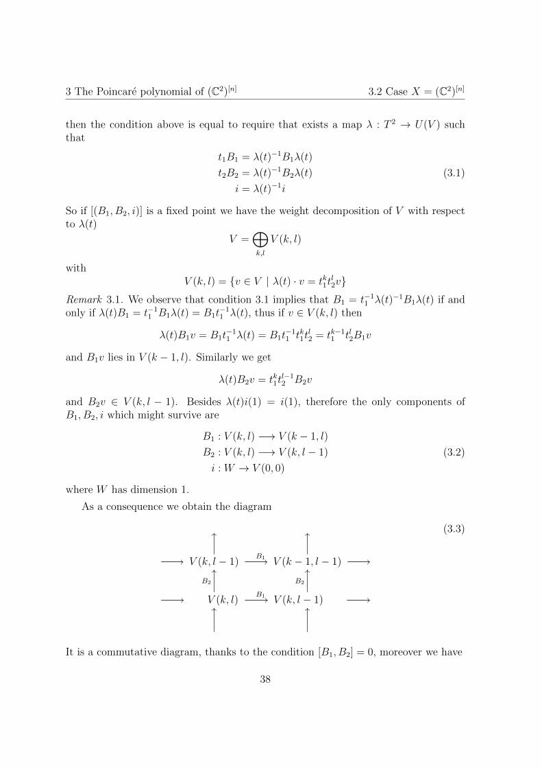
As a consequence we obtain the diagram
// V (k, l − 1)B1 //
OO
V (k − 1, l − 1)
OO
//
// V (k, l)B1 //
B2
OO
V (k, l − 1) //
B2
OO
OO OO
(3.3)
It is a commutative diagram, thanks to the condition [B1, B2] = 0, moreover we have
38
3.2 Case X = (C2)[n] 3 The Poincare polynomial of (C2)[n]
Proposition 3.2. The commutative diagram in 3.3 has the following properties:
1. If k > 0 or l > 0 then V (k, l) = 0
2. For every k, l ∈ Z, it holds dimV (k, l) ≤ 1
3. If k ≤ 0 and l ≤ 0 then dimV (k, l) ≥ dimV (k, l−1) and dimV (k, l) ≥ dimV (k−1, l).
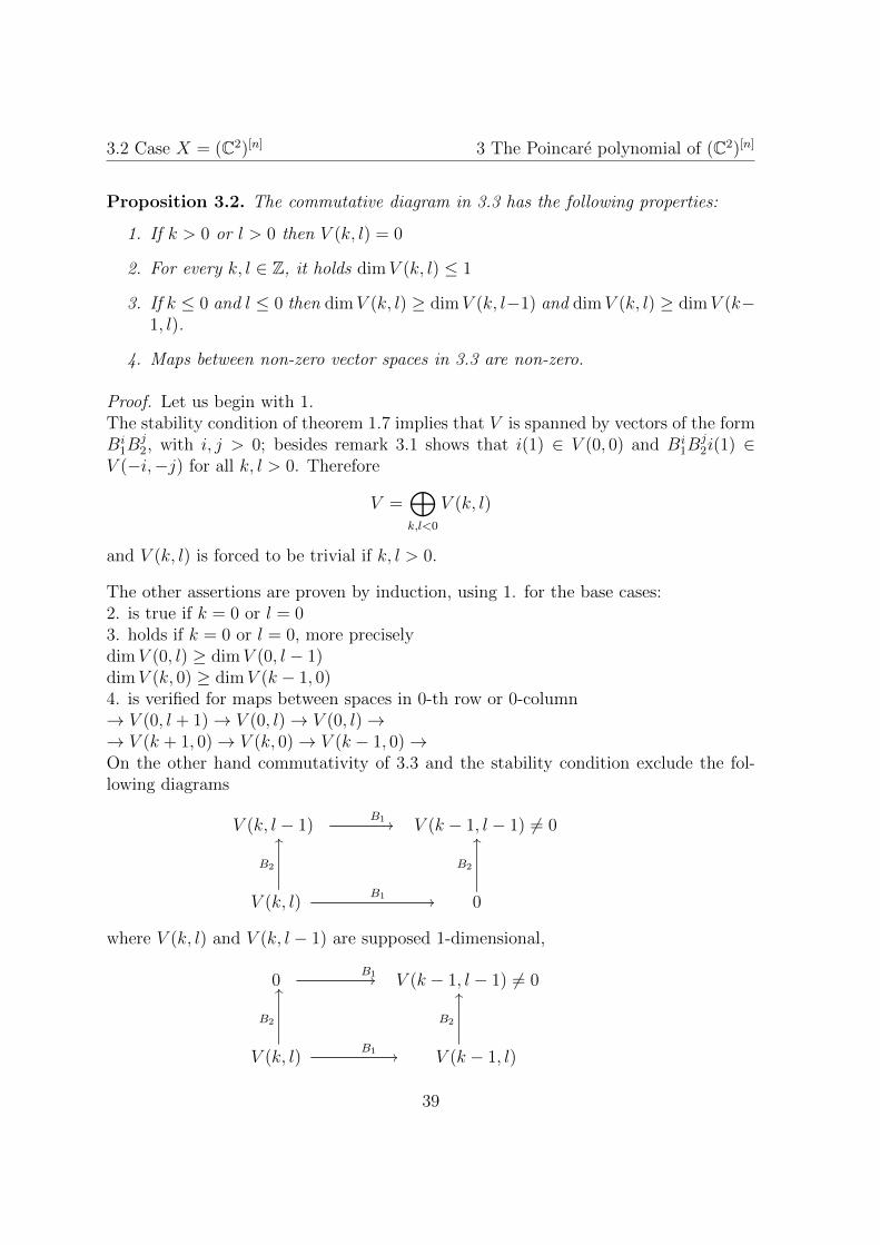
4. Maps between non-zero vector spaces in 3.3 are non-zero.
Proof. Let us begin with 1.The stability condition of theorem 1.7 implies that V is spanned by vectors of the formBi
1Bj2, with i, j > 0; besides remark 3.1 shows that i(1) ∈ V (0, 0) and Bi
1Bj2i(1) ∈
V (−i,−j) for all k, l > 0. Therefore
V =⊕k,l<0
V (k, l)
and V (k, l) is forced to be trivial if k, l > 0.
The other assertions are proven by induction, using 1. for the base cases:2. is true if k = 0 or l = 03. holds if k = 0 or l = 0, more preciselydimV (0, l) ≥ dimV (0, l − 1)dimV (k, 0) ≥ dimV (k − 1, 0)4. is verified for maps between spaces in 0-th row or 0-column→ V (0, l + 1)→ V (0, l)→ V (0, l)→→ V (k + 1, 0)→ V (k, 0)→ V (k − 1, 0)→On the other hand commutativity of 3.3 and the stability condition exclude the fol-lowing diagrams
V (k, l − 1)B1 // V (k − 1, l − 1) 6= 0
V (k, l)B1 //
B2
OO
0
B2
OO
where V (k, l) and V (k, l − 1) are supposed 1-dimensional,
0B1// V (k − 1, l − 1) 6= 0
V (k, l)B1 //
B2
OO
V (k − 1, l)
B2
OO
39
3 The Poincare polynomial of (C2)[n] 3.2 Case X = (C2)[n]
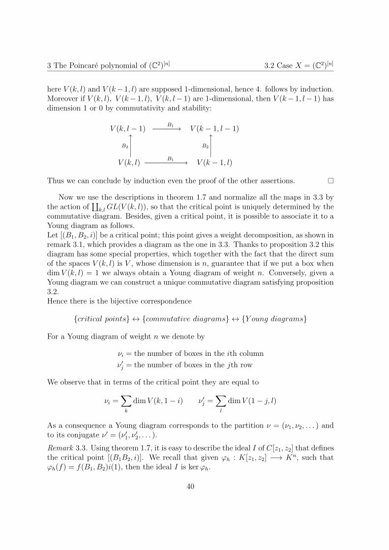
here V (k, l) and V (k−1, l) are supposed 1-dimensional, hence 4. follows by induction.Moreover if V (k, l), V (k− 1, l), V (k, l− 1) are 1-dimensional, then V (k− 1, l− 1) hasdimension 1 or 0 by commutativity and stability:
V (k, l − 1)B1 // V (k − 1, l − 1)
V (k, l)B1 //
B2
OO
V (k − 1, l)
B2
OO
Thus we can conclude by induction even the proof of the other assertions.
Now we use the descriptions in theorem 1.7 and normalize all the maps in 3.3 bythe action of
∐k,lGL(V (k, l)), so that the critical point is uniquely determined by the
commutative diagram. Besides, given a critical point, it is possible to associate it to aYoung diagram as follows.Let [(B1, B2, i)] be a critical point; this point gives a weight decomposition, as shown inremark 3.1, which provides a diagram as the one in 3.3. Thanks to proposition 3.2 thisdiagram has some special properties, which together with the fact that the direct sumof the spaces V (k, l) is V , whose dimension is n, guarantee that if we put a box whendimV (k, l) = 1 we always obtain a Young diagram of weight n. Conversely, given aYoung diagram we can construct a unique commutative diagram satisfying proposition3.2.Hence there is the bijective correspondence
critical points ↔ commutative diagrams ↔ Y oung diagrams
For a Young diagram of weight n we denote by
νi = the number of boxes in the ith column
ν ′j = the number of boxes in the jth row
We observe that in terms of the critical point they are equal to
νi =∑k
dimV (k, 1− i) ν ′j =∑l
dimV (1− j, l)
As a consequence a Young diagram corresponds to the partition ν = (ν1, ν2, . . . ) andto its conjugate ν ′ = (ν ′1, ν
′2, . . . ).
Remark 3.3. Using theorem 1.7, it is easy to describe the ideal I of C[z1, z2] that definesthe critical point [(B1B2, i)]. We recall that given ϕh : K[z1, z2] −→ Kn, such thatϕh(f) = f(B1, B2)i(1), then the ideal I is kerϕh.
40
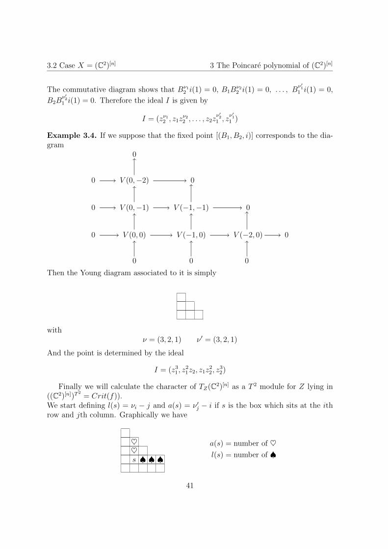
3.2 Case X = (C2)[n] 3 The Poincare polynomial of (C2)[n]
The commutative diagram shows that Bν12 i(1) = 0, B1B
ν22 i(1) = 0, . . . , B
ν′11 i(1) = 0,
B2Bν′21 i(1) = 0. Therefore the ideal I is given by
I = (zν12 , z1zν22 , . . . , z2z
ν′21 , z
ν′11 )
Example 3.4. If we suppose that the fixed point [(B1, B2, i)] corresponds to the dia-gram
0
0 // V (0,−2) //
OO
0
0 // V (0,−1) //
OO
V (−1,−1) //
OO
0
0 // V (0, 0)
OO
// V (−1, 0) //
OO
V (−2, 0) //
OO
0
0
OO
0
OO
0
OO
Then the Young diagram associated to it is simply
withν = (3, 2, 1) ν ′ = (3, 2, 1)
And the point is determined by the ideal
I = (z31 , z
21z2, z1z
22 , z
32)
Finally we will calculate the character of TZ(C2)[n] as a T 2 module for Z lying in((C2)[n])T
2= Crit(f)).
We start defining l(s) = νi − j and a(s) = ν ′j − i if s is the box which sits at the ithrow and jth column. Graphically we have
♥♥s ♠ ♠ ♠
a(s) = number of ♥l(s) = number of ♠
41
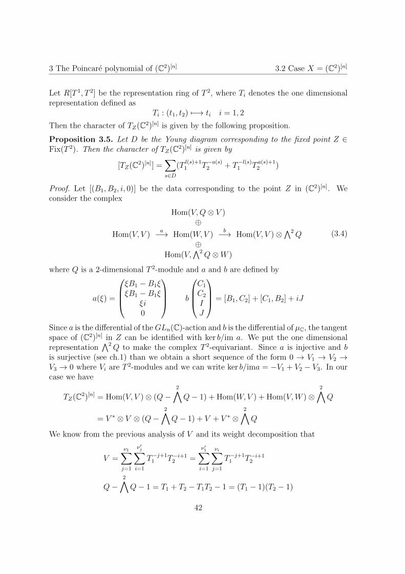
3 The Poincare polynomial of (C2)[n] 3.2 Case X = (C2)[n]
Let R[T 1, T 2] be the representation ring of T 2, where Ti denotes the one dimensionalrepresentation defined as
Ti : (t1, t2) 7−→ ti i = 1, 2
Then the character of TZ(C2)[n] is given by the following proposition.
Proposition 3.5. Let D be the Young diagram corresponding to the fixed point Z ∈Fix(T 2). Then the character of TZ(C2)[n] is given by
[TZ(C2)[n]] =∑s∈D
(Tl(s)+11 T
−a(s)2 + T
−l(s)1 T
a(s)+12 )
Proof. Let [(B1, B2, i, 0)] be the data corresponding to the point Z in (C2)[n]. Weconsider the complex
Hom(V,Q⊗ V )⊕
Hom(V, V )a−→ Hom(W,V )
b−→ Hom(V, V )⊗∧2Q
⊕Hom(V,
∧2Q⊗W )
(3.4)
where Q is a 2-dimensional T 2-module and a and b are defined by
a(ξ) =
ξB1 −B1ξξB1 −B1ξ
ξi0
b
C1
C2
IJ
= [B1, C2] + [C1, B2] + iJ
Since a is the differential of theGLn(C)-action and b is the differential of µC, the tangentspace of (C2)[n] in Z can be identified with ker b/im a. We put the one dimensionalrepresentation
∧2Q to make the complex T 2-equivariant. Since a is injective and bis surjective (see ch.1) than we obtain a short sequence of the form 0 → V1 → V2 →V3 → 0 where Vi are T 2-modules and we can write ker b/ima = −V1 + V2 − V3. In ourcase we have
TZ(C2)[n] = Hom(V, V )⊗ (Q−2∧Q− 1) + Hom(W,V ) + Hom(V,W )⊗
2∧Q
= V ∗ ⊗ V ⊗ (Q−2∧Q− 1) + V + V ∗ ⊗
2∧Q
We know from the previous analysis of V and its weight decomposition that
V =
ν1∑j=1
ν′j∑i=1
T−j+11 T−i+1
2 =
ν′1∑i=1
νi∑j=1
T−j+11 T−i+1
2
Q−2∧Q− 1 = T1 + T2 − T1T2 − 1 = (T1 − 1)(T2 − 1)
42
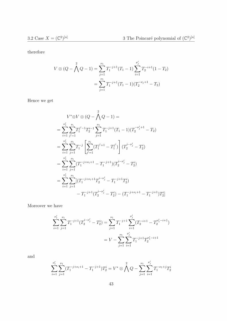
3.2 Case X = (C2)[n] 3 The Poincare polynomial of (C2)[n]
therefore
V ⊗ (Q−2∧Q− 1) =
ν1∑j=1
T−j+11 (T1 − 1)
ν′j∑i=1
T−i+12 (1− T2)
=
ν1∑j=1
T−j+11 (T1 − 1)(T
−νj+12 − T2)
Hence we get
V ∗⊗V ⊗ (Q−2∧Q− 1) =
=
ν′1∑i=1
νi∑j′=1
T j′−1
1 T i−12
ν1∑j=1
T−j+11 (T1 − 1)(T
−ν′j+1
2 − T2)
=
ν′1∑i=1
ν1∑j=1
T−j1
[νi∑j′=1
(T j′+1
1 − T j′
1 )
](T
i−ν′j2 − T i2)
=
ν′1∑i=1
ν1∑j=1
(T−j+νi+11 − T−j+1
1 )(Ti−ν′j2 − T i2)
=
ν′1∑i=1
ν1∑j=1
[(T−j+νi+11 T
i−ν′j2 − T−j+1
1 T i2)
− T−j+11 (T
i−ν′j2 − T i2)− (T−j+νi+1
1 − T−j+11 )T i2]
Moreover we have
ν′1∑i=1
ν1∑j=1
T−j+11 (T
i−ν′j2 − T i2) =
ν1∑j=1
T−j+11
ν′j∑i=1
(T−i+12 − T ν
′1−i+1
2 )
= V −ν1∑j=1
ν′j∑i=1
T−j+11 T
ν′1−i+12
and
ν′1∑i=1
ν1∑j=1
(T−j+νi+11 − T−j+1
1 )T i2 = V ∗ ⊗2∧Q−
ν1∑j=1
ν′j∑i=1
T−ν1+j1 T i2
43
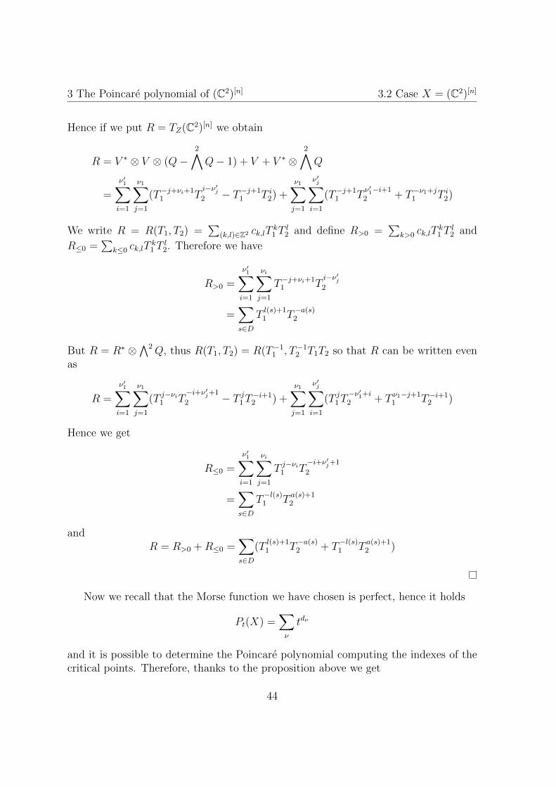
3 The Poincare polynomial of (C2)[n] 3.2 Case X = (C2)[n]
Hence if we put R = TZ(C2)[n] we obtain
R = V ∗ ⊗ V ⊗ (Q−2∧Q− 1) + V + V ∗ ⊗
2∧Q
=
ν′1∑i=1
ν1∑j=1
(T−j+νi+11 T
i−ν′j2 − T−j+1
1 T i2) +
ν1∑j=1
ν′j∑i=1
(T−j+11 T
ν′1−i+12 + T−ν1+j
1 T i2)
We write R = R(T1, T2) =∑
(k,l)∈Z2 ck,lTk1 T
l2 and define R>0 =
∑k>0 ck,lT
k1 T
l2 and
R≤0 =∑
k≤0 ck,lTk1 T
l2. Therefore we have
R>0 =
ν′1∑i=1
νi∑j=1
T−j+νi+11 T
i−ν′j2
=∑s∈D
Tl(s)+11 T
−a(s)2
But R = R∗ ⊗∧2Q, thus R(T1, T2) = R(T−1
1 , T−12 T1T2 so that R can be written even
as
R =
ν′1∑i=1
ν1∑j=1
(T j−νi1 T−i+ν′j+1
2 − T j1T−i+12 ) +
ν1∑j=1
ν′j∑i=1
(T j1T−ν′1+i2 + T ν1−j+1
1 T−i+12 )
Hence we get
R≤0 =
ν′1∑i=1
νi∑j=1
T j−νi1 T−i+ν′j+1
2
=∑s∈D
T−l(s)1 T
a(s)+12
andR = R>0 +R≤0 =
∑s∈D
(Tl(s)+11 T
−a(s)2 + T
−l(s)1 T
a(s)+12 )
Now we recall that the Morse function we have chosen is perfect, hence it holds
Pt(X) =∑ν
tdν
and it is possible to determine the Poincare polynomial computing the indexes of thecritical points. Therefore, thanks to the proposition above we get
44
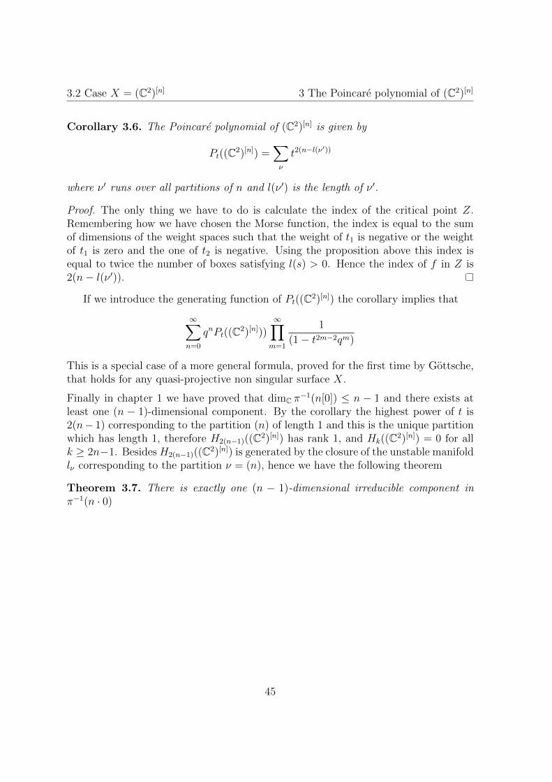
3.2 Case X = (C2)[n] 3 The Poincare polynomial of (C2)[n]
Corollary 3.6. The Poincare polynomial of (C2)[n] is given by
Pt((C2)[n]) =∑ν
t2(n−l(ν′))
where ν ′ runs over all partitions of n and l(ν ′) is the length of ν ′.
Proof. The only thing we have to do is calculate the index of the critical point Z.Remembering how we have chosen the Morse function, the index is equal to the sumof dimensions of the weight spaces such that the weight of t1 is negative or the weightof t1 is zero and the one of t2 is negative. Using the proposition above this index isequal to twice the number of boxes satisfying l(s) > 0. Hence the index of f in Z is2(n− l(ν ′)).
If we introduce the generating function of Pt((C2)[n]) the corollary implies that
∞∑n=0
qnPt((C2)[n]))∞∏m=1
1
(1− t2m−2qm)
This is a special case of a more general formula, proved for the first time by Gottsche,that holds for any quasi-projective non singular surface X.
Finally in chapter 1 we have proved that dimC π−1(n[0]) ≤ n − 1 and there exists at
least one (n − 1)-dimensional component. By the corollary the highest power of t is2(n− 1) corresponding to the partition (n) of length 1 and this is the unique partitionwhich has length 1, therefore H2(n−1)((C2)[n]) has rank 1, and Hk((C2)[n]) = 0 for allk ≥ 2n−1. Besides H2(n−1)((C2)[n]) is generated by the closure of the unstable manifoldlν corresponding to the partition ν = (n), hence we have the following theorem
Theorem 3.7. There is exactly one (n − 1)-dimensional irreducible component inπ−1(n · 0)
45

Ringraziamenti
Il primo grazie va al il Professor Luca Migliorini per la disponibilita, l’attenzione ela pazienza con cui mi ha seguito, anche da lontano, e per tutto quello che mi hainsegnato.Grazie a Camilla e Marco per i preziosi consigli e suggerimenti.Un grazie comune va ad i miei amici ed amiche, in particolare a Marta, a (l’altra)Marta, a Sara che con me hanno condiviso i momenti di sconforto (si, ci sono stati),quelli di ansia (Sara?) e quelli (molto piu numerosi) di gioia: avete reso questi anni aBologna piu leggeri e spensierati, piu ricchi e indimenticabili!A Ferdinando: grazie.
47


Bibliography
[1] M.F. Atiyah and R. Bott, The Yang-Mills equations over Riemann surfaces, Phil.Trans. Roy. Soc. London A 308 (1982), 524-615
[2] W. Barth, Moduli of bundles on the projective plane, Invent. Math. 42 (1977),63-91
[3] A. Beauville, Variete khalriennes dont la premiere classe de Chern est nulle, J. ofDiferential Geom. 18 (1983), 755-782
[4] D. Birkes, Orbits of linear algebraic groups, Ann. of Math 93 (1971), 459-473
[5] M.A. de Cataldo and L. Migliorini, the Douady space of a complex surface, Ad-vanced in Mathematics, 151, 283-321 (2000)
[6] B.Fantechi, L. Gottsche, L. Illusie, S. L. Kleiman, N. Nitsure, and A. Vistoli Fun-damental Algebraic Geometry: Grothendieck’s FGA Explained, American Mathe-matical Society, 2005
[7] L. Gottsche Hilbert schemes of zero-dimensional subschemes of smooth varieties,Lecture Notes in Mathematics, 1572. Springer-Verlag, Berlin 1994
[8] A. Grothendieck, Techniques de construction et theore d’extistence en geometriealgebrique, IV: Les schemas de Hilbert, Seminaire Bourbaki expose 221 (1961);IHP, Paris
[9] N,J. Hitchin, A. Karlhede, U. Lindstrom and M. Rocek, Hyperkahler metrics andsupersimmetry Comm Math. Phys. 108 (1987), 535-589
[10] S.Kobayashi and K. Nomizu, Foundations of differential geometry, vols I,II. Wiley,New York, 1963, 1969
[11] D. Luna, Slices Etales, Bull. Soc. Math. France 33 (1973), 81-105
[12] J. Milnor Morse theory, based on lecture notes by M. Spivak and R. Wells, Prince-ton University Press, 1963
49

BIBLIOGRAPHY BIBLIOGRAPHY
[13] D. Mumford, J. Fogarty Geometric invariant theory, Springer, 1982
[14] H. Nakajima, Lectures on Hilbert Schemes of Points on Surfaces, American Math-ematical Society, 1999
[15] P.E. Newstead, Introduction to moduli problems and orbit spaces, Tata InstituteLectures, 51, Springer-Verlag, 1978
[16] Thomas, R. P. Notes on GIT and symplectic reduction for bundles and varieties,Surveys in Differential Geometry, 10 (2006): A Tribute to Professor S.-S. Chern.arXiv:math/0512411.
50