The Phenomenology of Large Scale Structure

• Motivation: A biased view of dark matters• Gravitational Instability

– The spherical collapse model– Tri-axial (ellipsoidal) collapse

• The random-walk description– The halo mass function– Halo progenitors, formation, and merger trees– Environmental effects in hierarchical models– (SDSS galaxies and their environment)

• The Halo Model

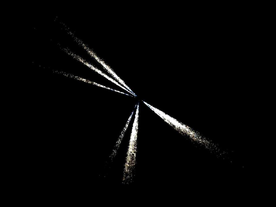
Galaxy clustering depends on type

Large samples (SDSS, 2dF) now available to quantify this

You can observe a lot just by watching. -Yogi Berra

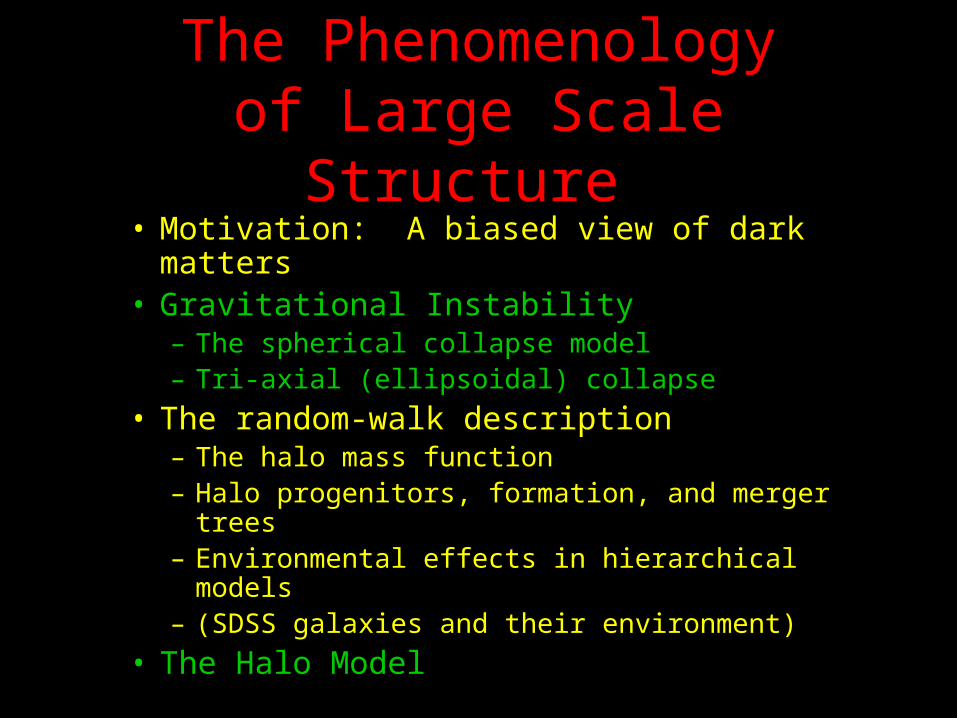
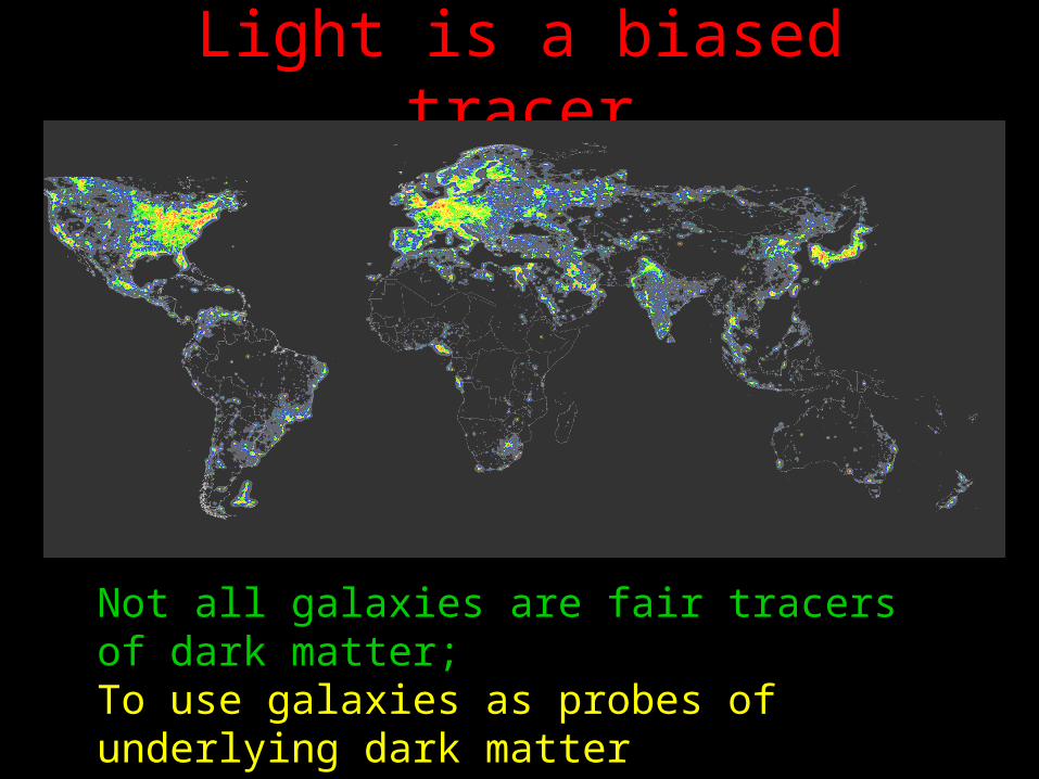
Light is a biased tracer

Not all galaxies are fair tracers of dark matter;To use galaxies as probes of underlying dark matter distribution, must understand ‘bias’

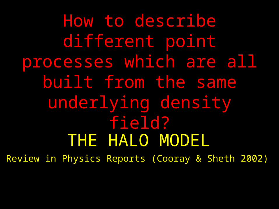
How to describe different point processes which are all built from the same underlying density field?

THE HALO MODELReview in Physics Reports (Cooray & Sheth 2002)

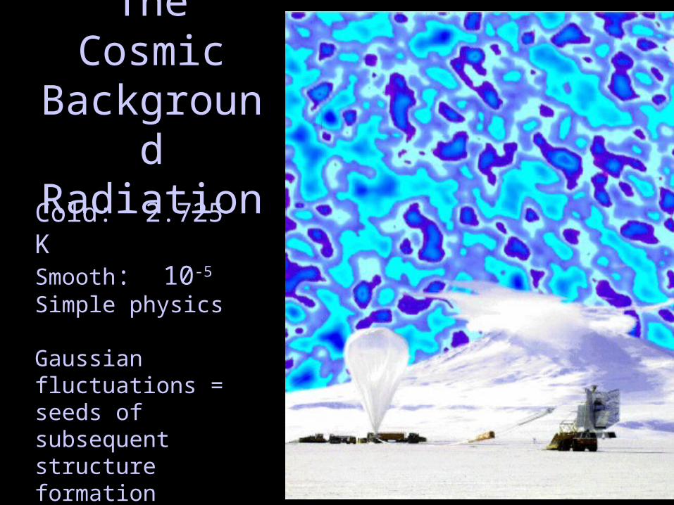
The Cosmic Background

Radiation

Cold: 2.725 KSmooth: 10-5

Simple physics

Gaussian fluctuations = seeds of subsequent structure formation = simple(r) mathLogic which follows is general

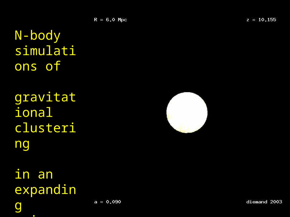
N-body simulations of

gravitational clustering

in an expanding universe

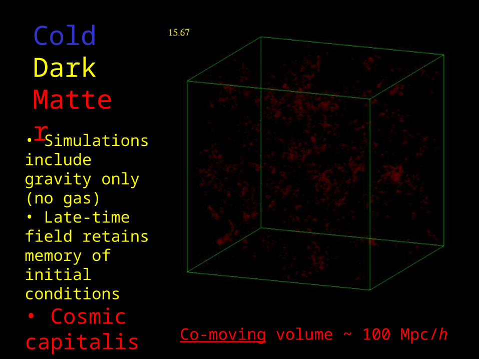
Cold Dark Matter

• Simulations include gravity only (no gas) • Late-time field retains memory of initial conditions

• Cosmic capitalism

Co-moving volume ~ 100 Mpc/h

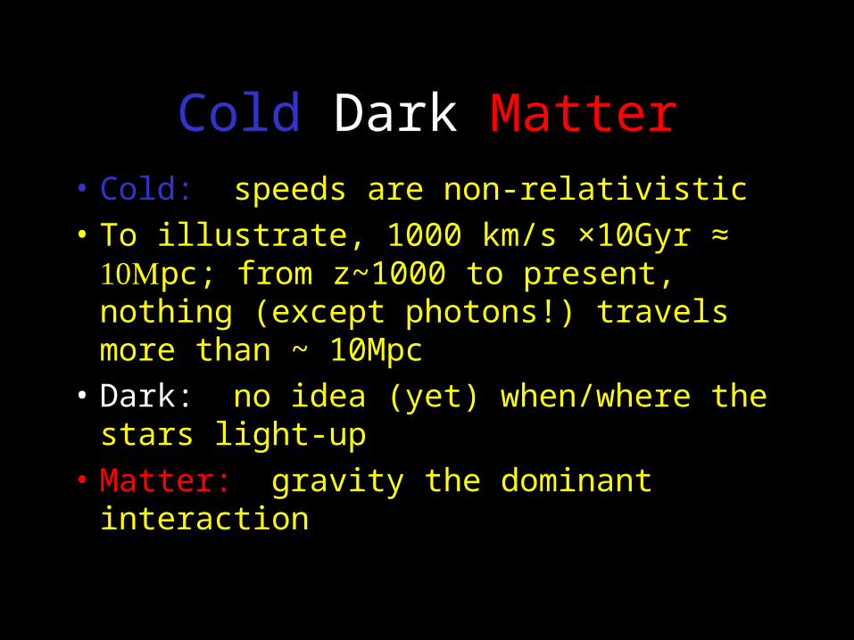
Cold Dark Matter

• Cold: speeds are non-relativistic

• To illustrate, 1000 km/s ×10Gyr ≈ pc; from z~1000 to present, nothing (except photons!) travels more than ~ 10Mpc

• Dark: no idea (yet) when/where the stars light-up

• Matter: gravity the dominant interaction

Models of halo abundances and clustering:

Gravity in an expanding universe

Goal:Use knowledge of initial conditions (CMB) to make inferences about

late-time, nonlinear structures

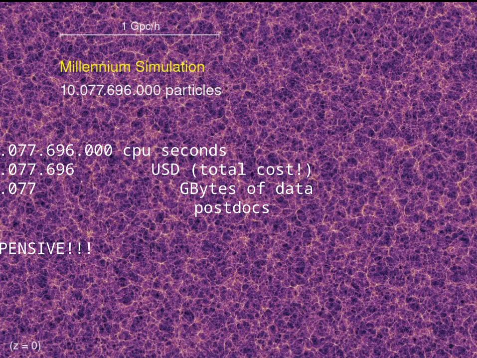
10.077.696.000 cpu seconds10.077.696 USD (total cost!)10.077 GBytes of data10 postdocs

EXPENSIVE!!!

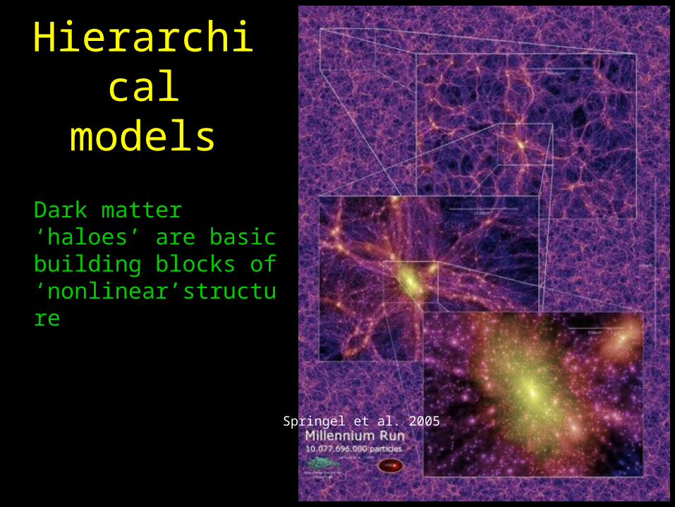
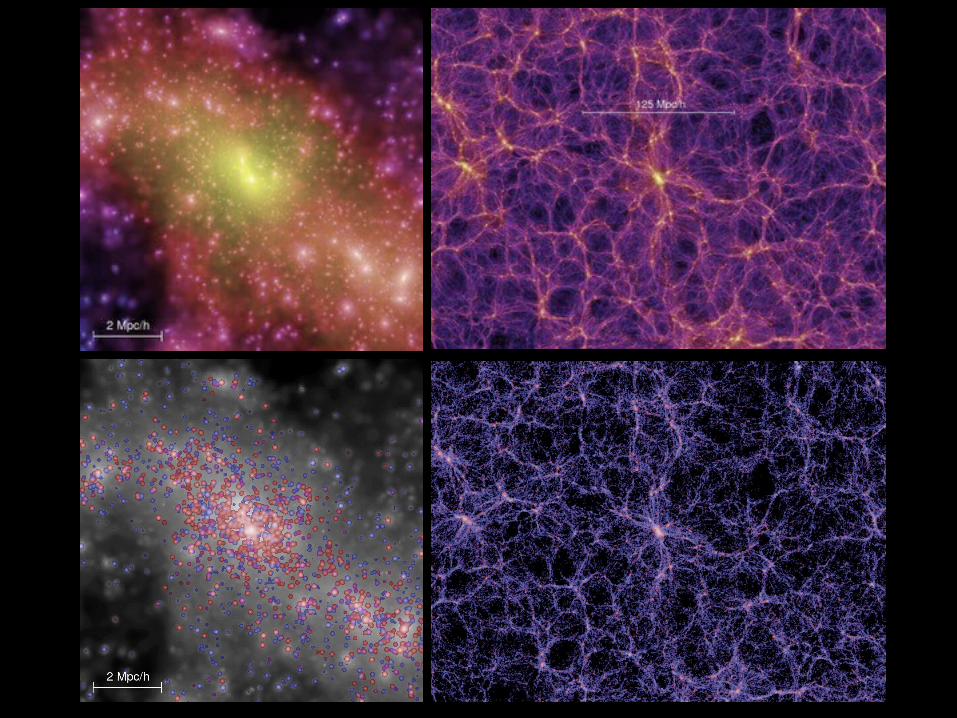
Hierarchical models

Springel et al. 2005

Dark matter ‘haloes’ are basic building blocks of ‘nonlinear’structure

MODELS OF NONLINEAR COLLAPSE

Assume a spherical cow….

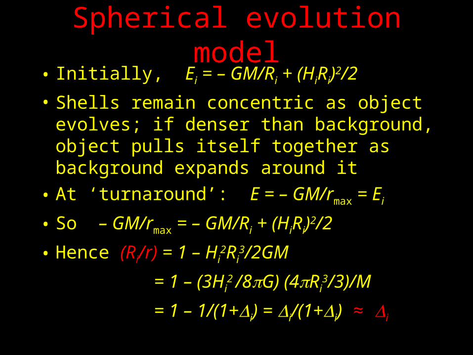
Spherical evolution model• Initially, Ei = – GM/Ri + (HiRi)2/2

• Shells remain concentric as object evolves; if denser than background, object pulls itself together as background expands around it

• At ‘turnaround’: E = – GM/rmax = Ei

• So – GM/rmax = – GM/Ri + (HiRi)2/2

• Hence (Ri/r) = 1 – Hi2Ri

3/2GM

= 1 – (3Hi2 /8G) (4Ri

3/3)/M

= 1 – 1/(1+i) = i/(1+i) ≈ i

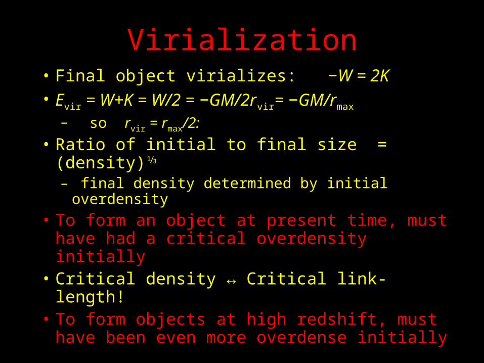
Virialization• Final object virializes: −W = 2K• Evir = W+K = W/2 = −GM/2rvir= −GM/rmax

– so rvir = rmax/2:

• Ratio of initial to final size = (density)⅓ – final density determined by initial overdensity

• To form an object at present time, must have had a critical overdensity initially

• Critical density ↔ Critical link-length! • To form objects at high redshift, must have

been even more overdense initially

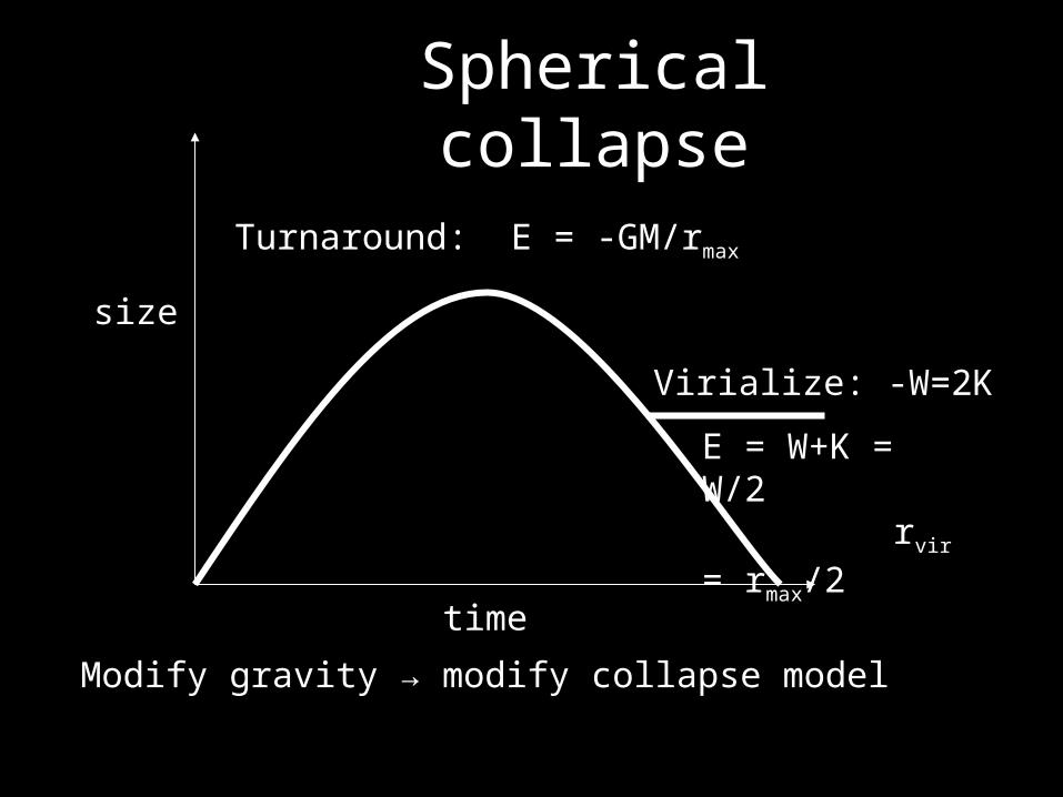
Spherical collapse

size

time

Turnaround: E = -GM/rmax

Virialize: -W=2K

E = W+K = W/2 rvir = rmax/2

Modify gravity → modify collapse model

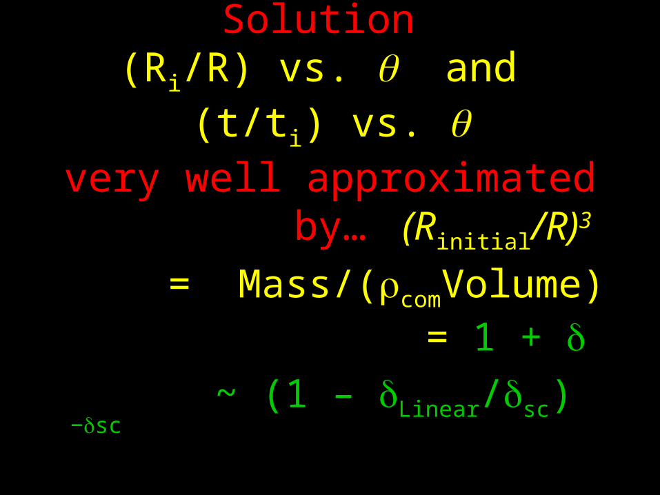
Exact Parametric Solution (Ri/R) vs. and (t/ti) vs.

very well approximated by…

(Rinitial/R)3

= Mass/(comVolume) = 1 +

~ (1 – Linear/sc)−sc

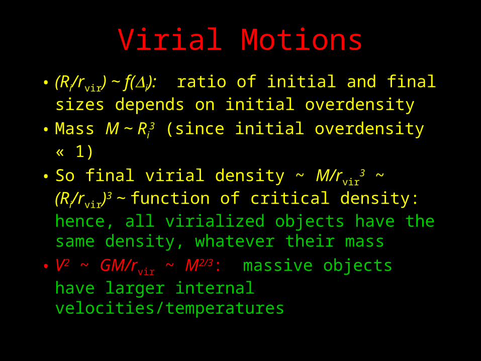
Virial Motions

• (Ri/rvir) ~ f(i): ratio of initial and final sizes depends on initial overdensity

• Mass M ~ Ri3 (since initial overdensity « 1)

• So final virial density ~ M/rvir3 ~ (Ri/rvir)3 ~

function of critical density: hence, all virialized objects have the same density, whatever their mass

• V2 ~ GM/rvir ~ M2/3: massive objects have larger internal velocities/temperatures

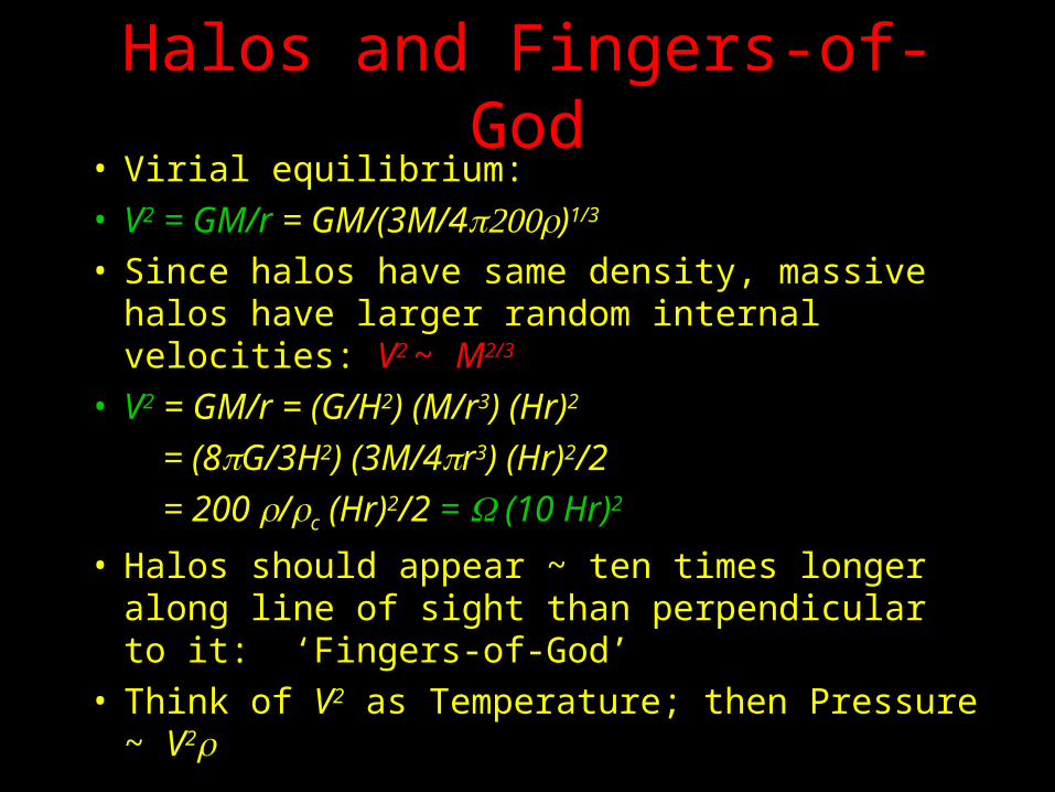
Halos and Fingers-of-God• Virial equilibrium: • V2 = GM/r = GM/(3M/4)1/3

• Since halos have same density, massive halos have larger random internal velocities: V2 ~ M2/3

• V2 = GM/r = (G/H2) (M/r3) (Hr)2

= (8G/3H2) (3M/4r3) (Hr)2/2

= 200 /c (Hr)2/2 = (10 Hr)2

• Halos should appear ~ ten times longer along line of sight than perpendicular to it: ‘Fingers-of-God’

• Think of V2 as Temperature; then Pressure ~ V2

HALO ABUNDANCES

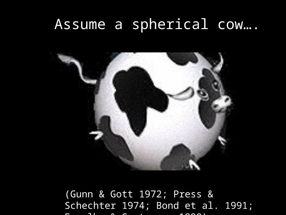
Assume a spherical cow….

(Gunn & Gott 1972; Press & Schechter 1974; Bond et al. 1991; Fosalba & Gaztanaga 1998)

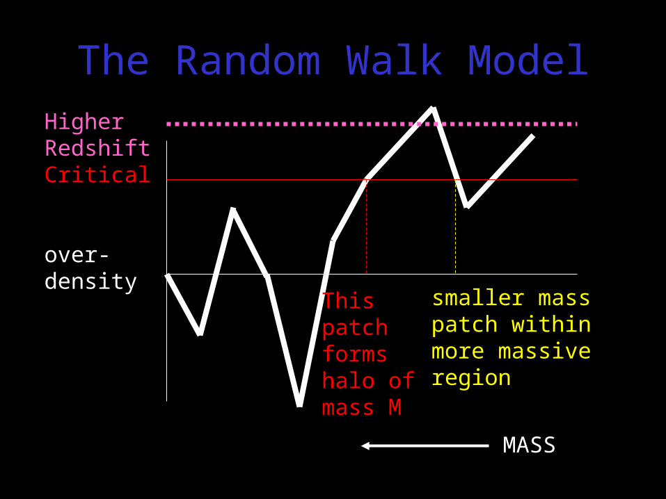
Higher RedshiftCritical

over-density

MASS

smaller mass patch within more massive region

This patch forms halo of mass M

The Random Walk Model

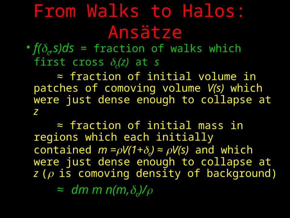
From Walks to Halos: Ansätze

• f(c,s)ds = fraction of walks which first crossc(z) at s

≈ fraction of initial volume in patches of comoving volume V(s) which were just dense enough to collapse at z

≈ fraction of initial mass in regions which each initially contained m =V(1+c) ≈ V(s) and which were just dense enough to collapse at z (is comoving density of background)

≈ dm m n(m,c)/

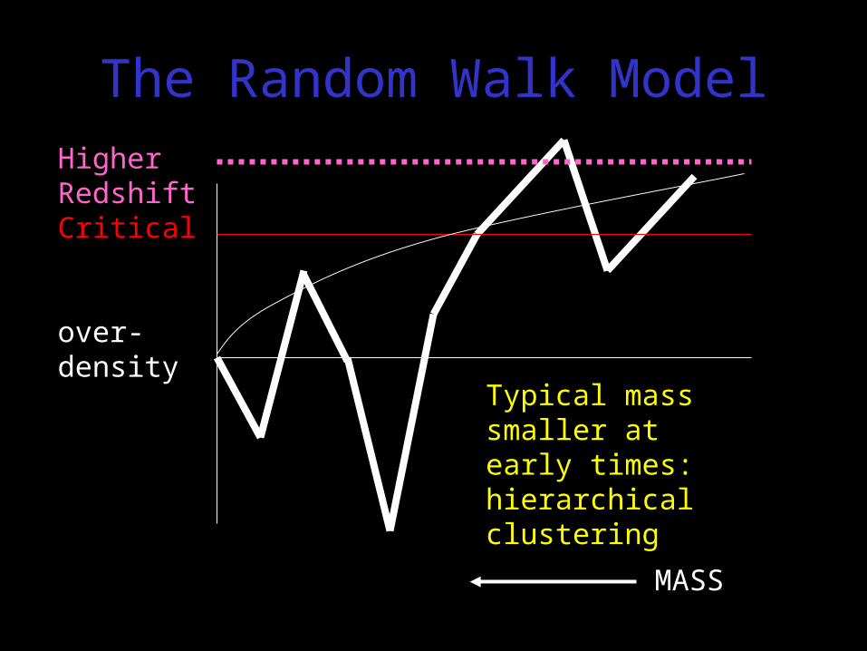
Higher RedshiftCritical

over-density

MASS

Typical mass smaller at early times: hierarchical clustering

The Random Walk Model

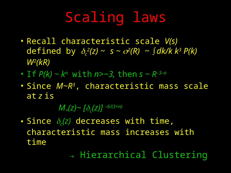
Scaling laws

• Recall characteristic scale V(s) defined by c

2(z) ~ s ~ 2(R) ~ ∫dk/k k3 P(k) W2(kR)

• If P(k) ~ kn with n>−3, then s ~ R–3–n

• Since M~R3, characteristic mass scale at z is

M*(z)~ [c(z)] –6/(3+n)

• Since c(z) decreases with time, characteristic mass increases with time

→ Hierarchical Clustering

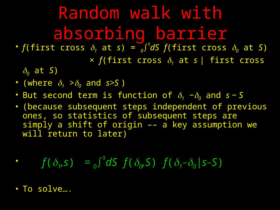
Random walk with absorbing barrier• f(first cross 1 at s) = 0∫

sdS f(first cross 0 at S)

× f(first cross 1 at s | first cross 0 at S) • (where 1 >0 and s>S )• But second term is function of 1 −0 and s − S • (because subsequent steps independent of previous ones,

so statistics of subsequent steps are simply a shift of origin –– a key assumption we will return to later)

• f(1,s) = 0∫sdS f(0,S) f(1−0|s−S)

• To solve….

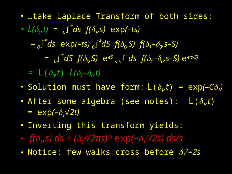
• …take Laplace Transform of both sides:

• L(1,t) = 0∫∞ds f(1,s) exp(–ts)

= 0∫∞ds exp(–ts) 0∫

sdS f(0,S) f(1–0,s–S)

= 0∫∞dS f(0,S) e-tS s-S∫

∞ds f(1–0,s–S) e-t(s-S)

= L(0,t) L(1–0,t)

• Solution must have form: L(1,t) = exp(–C1)

• After some algebra (see notes): L(1,t) = exp(–1√2t)

• Inverting this transform yields:

• f(1,s) ds = (12/2πs)½ exp(–1

2/2s) ds/s

• Notice: few walks cross before 12=2s

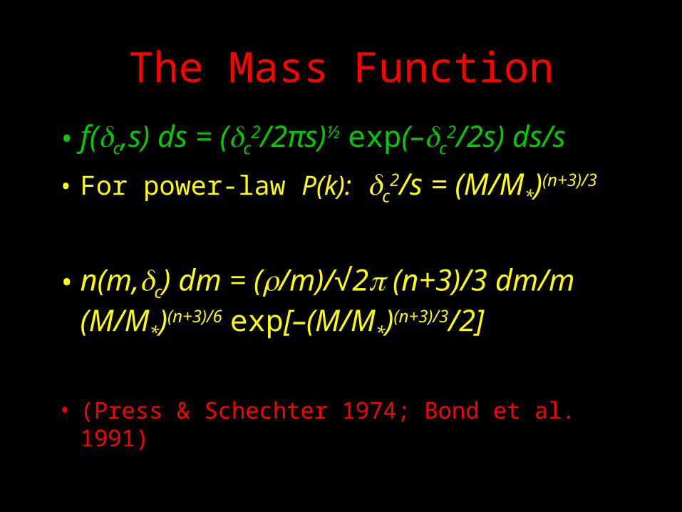
The Mass Function

• f(c,s) ds = (c2/2πs)½ exp(–c

2/2s) ds/s

• For power-law P(k): c2/s = (M/M*)(n+3)/3

• n(m,c) dm = (/m)/√2 (n+3)/3 dm/m (M/M*)(n+3)/6 exp[–(M/M*)(n+3)/3/2]

• (Press & Schechter 1974; Bond et al. 1991)

Simplification because…

• Everything local• Evolution determined by cosmology

(competition between gravity and expansion)

• Statistics determined by initial fluctuation field: since Gaussian, statistics specified by initial power-spectrum P(k)

• Fact that only very fat cows are spherical is a detail (crucial for precision cosmology)

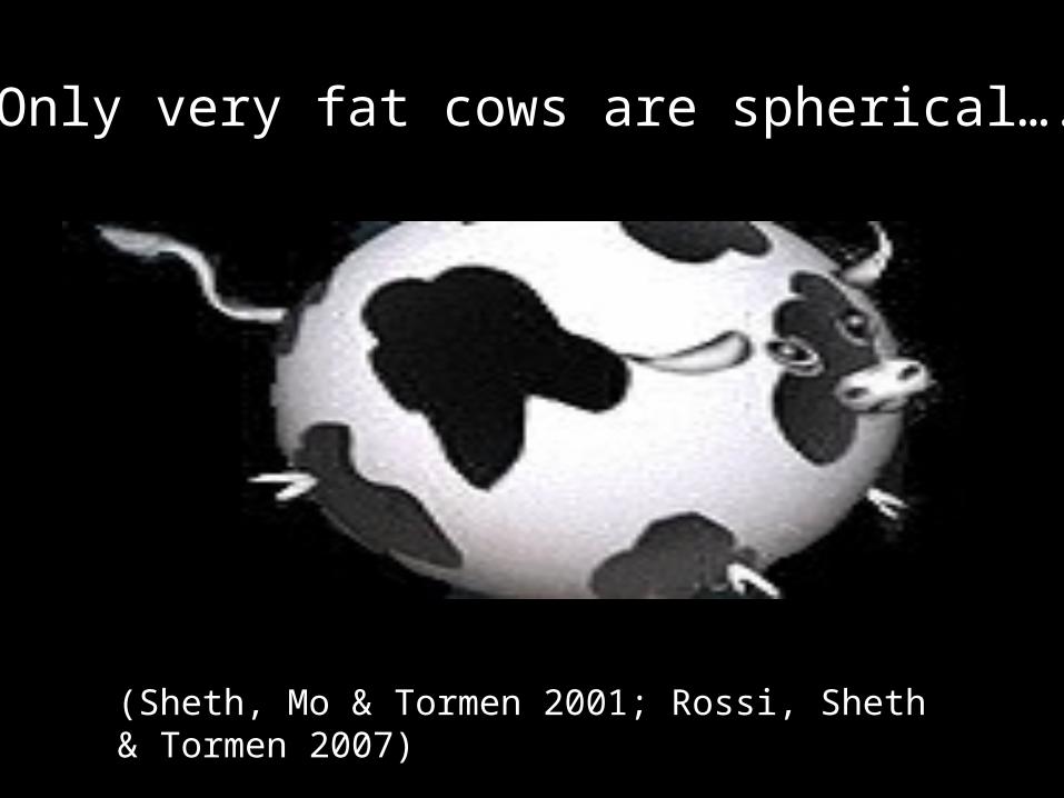
Only very fat cows are spherical….

(Sheth, Mo & Tormen 2001; Rossi, Sheth & Tormen 2007)

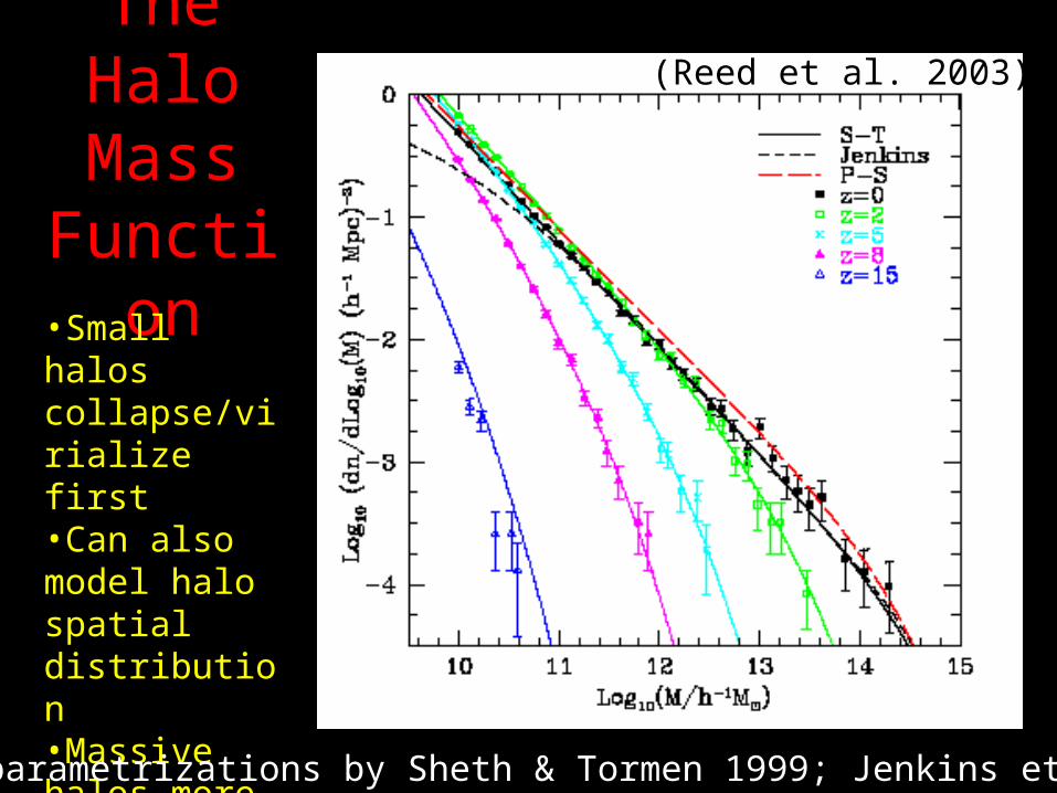
The Halo Mass

Function•Small halos collapse/virialize first•Can also model halo spatial distribution•Massive halos more strongly clustered

(Reed et al. 2003)

(current parametrizations by Sheth & Tormen 1999; Jenkins etal. 2001)

Theory predicts…• Can rescale halo abundances to ‘universal’

form, independent of P(k), z, cosmology– Greatly simplifies likelihood analyses

• Intimate connection between abundance and clustering of dark halos– Can use cluster clustering as check that cluster

mass-observable relation correctly calibrated

• Important to test if these fortunate simplifications also hold at 1% precision

(Sheth & Tormen 1999)

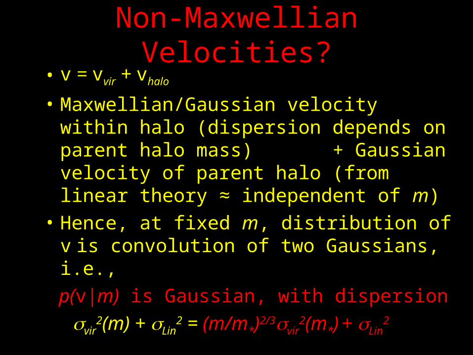
Non-Maxwellian Velocities?• v = vvir + vhalo

• Maxwellian/Gaussian velocity within halo (dispersion depends on parent halo mass) + Gaussian velocity of parent halo (from linear theory ≈ independent of m)

• Hence, at fixed m, distribution of v is convolution of two Gaussians, i.e.,

p(v|m) is Gaussian, with dispersion

vir2(m) + Lin

2 = (m/m*)2/3vir2(m*) + Lin

2

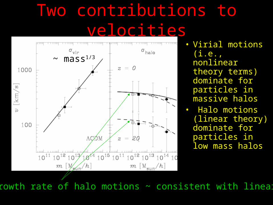
Two contributions to velocities• Virial motions

(i.e., nonlinear theory terms) dominate for particles in massive halos

• Halo motions (linear theory) dominate for particles in low mass halos

Growth rate of halo motions ~ consistent with linear theory

~ mass1/3

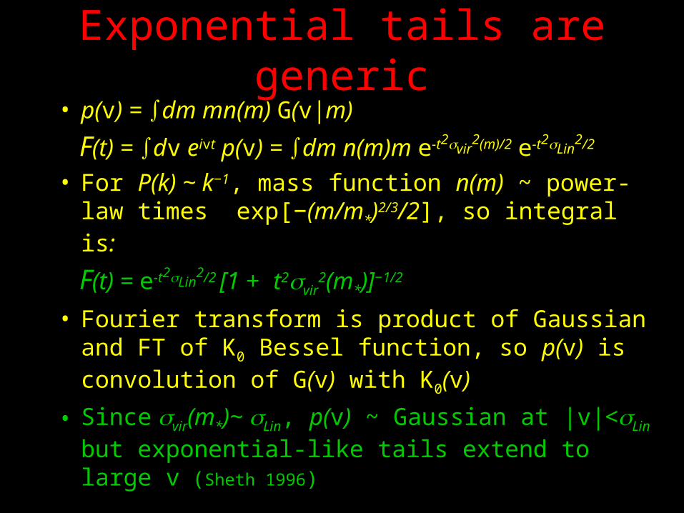
Exponential tails are generic• p(v) = ∫dm mn(m) G(v|m)

F(t) = ∫dv eivt p(v) = ∫dm n(m)m e-t2vir2(m)/2 e-t2Lin

2/2

• For P(k) ~ k−1, mass function n(m) ~ power-law times exp[−(m/m*)2/3/2], so integral is:

F(t) = e-t2Lin2/2 [1 + t2vir

2(m*)]−1/2

• Fourier transform is product of Gaussian and FT of K0 Bessel function, so p(v) is convolution of G(v) with K0(v)

• Since vir(m*)~ Lin, p(v) ~ Gaussian at |v|<Lin but exponential-like tails extend to large v (Sheth 1996)

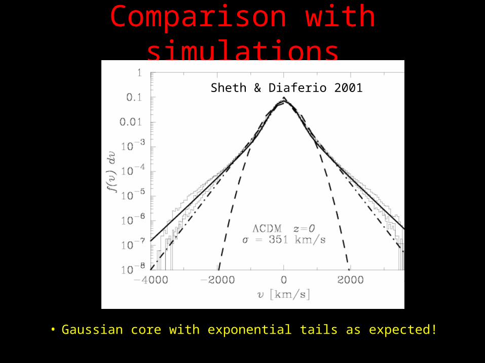
Comparison with simulations

• Gaussian core with exponential tails as expected!

Sheth & Diaferio 2001

EVOLUTIONAND

ENVIRONMENT

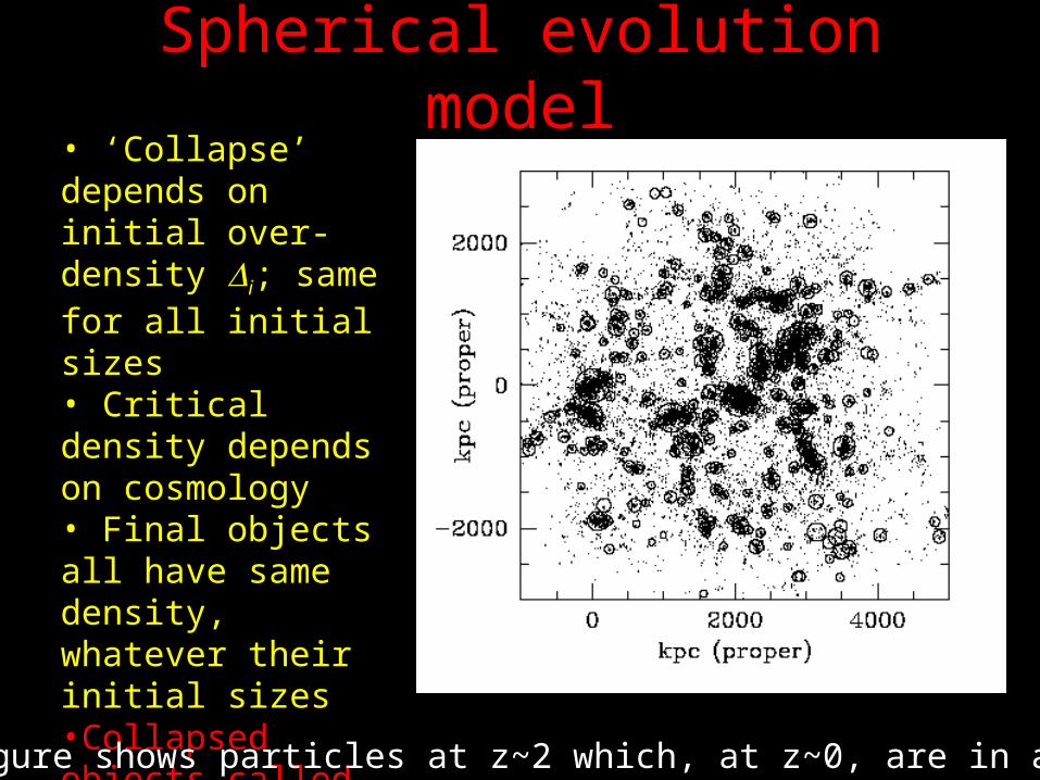
Spherical evolution model• ‘Collapse’ depends on initial over-density i; same for all initial sizes• Critical density depends on cosmology• Final objects all have same density, whatever their initial sizes•Collapsed objects called halos; ~ 200× denser than background, whatever their mass

(Figure shows particles at z~2 which, at z~0, are in a cluster)

Assume a spherical herd of spherical cows…

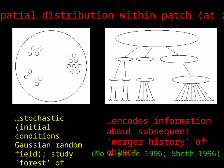
Initial spatial distribution within patch (at z~1000)...

…stochastic (initial conditions Gaussian random field); study `forest’ of merger history ‘trees’.

…encodes information about subsequent ‘merger history’ of object(Mo & White 1996; Sheth 1996)

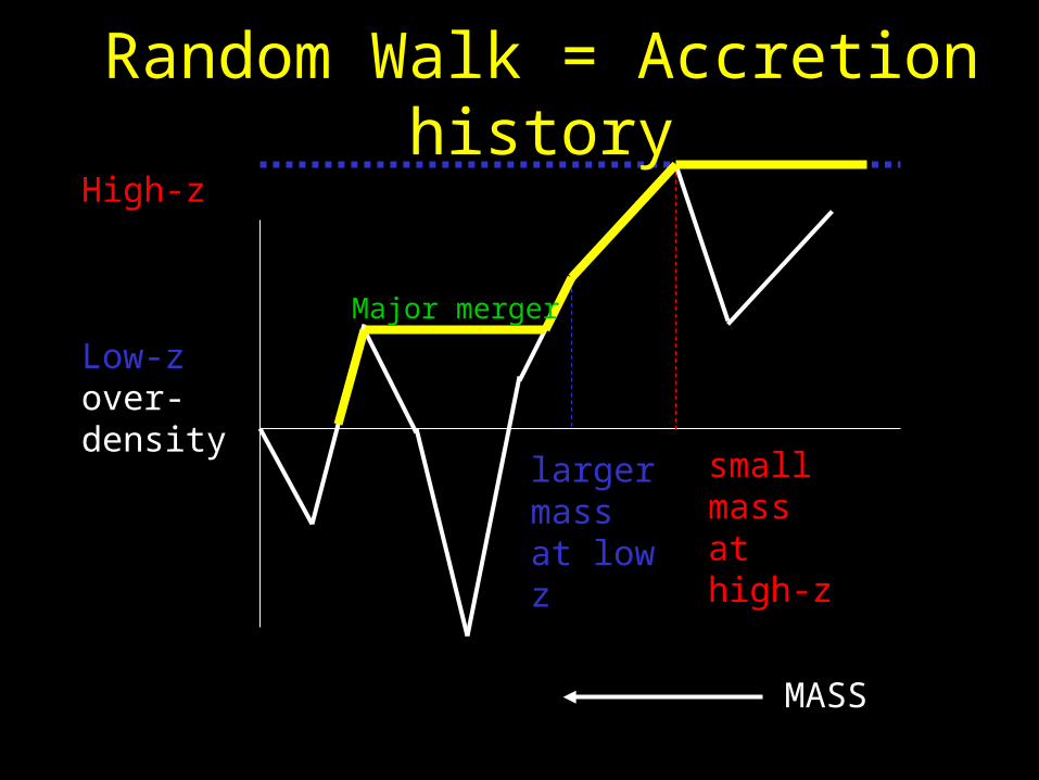
High-z

Low-zover-density

MASS

small mass at high-z

larger mass at low z

Random Walk = Accretion history

Major merger

Other features of the model

• Quantify forest of merger histories as function of halo mass (formation times, mass accretion, etc.)

• Model spatial distribution of halos: (halo clustering/biasing)– Abundance + clustering calibrates Mass

• Halos and their environment: – Nature vs. nurture—key to simplifying models

of galaxy formation

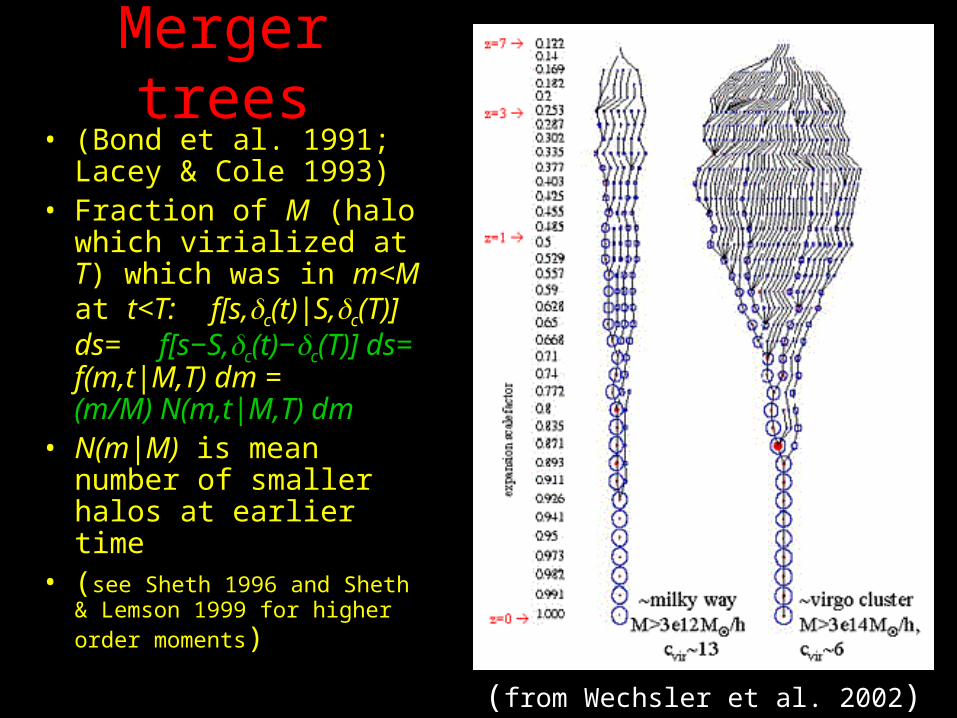
Merger trees• (Bond et al. 1991; Lacey

& Cole 1993)• Fraction of M (halo which

virialized at T) which was in m<M at t<T: f[s,c(t)|S,c(T)] ds= f[s−S,c(t)−c(T)] ds= f(m,t|M,T) dm = (m/M) N(m,t|M,T) dm

• N(m|M) is mean number of smaller halos at earlier time

• (see Sheth 1996 and Sheth & Lemson 1999 for higher order moments)

(from Wechsler et al. 2002)

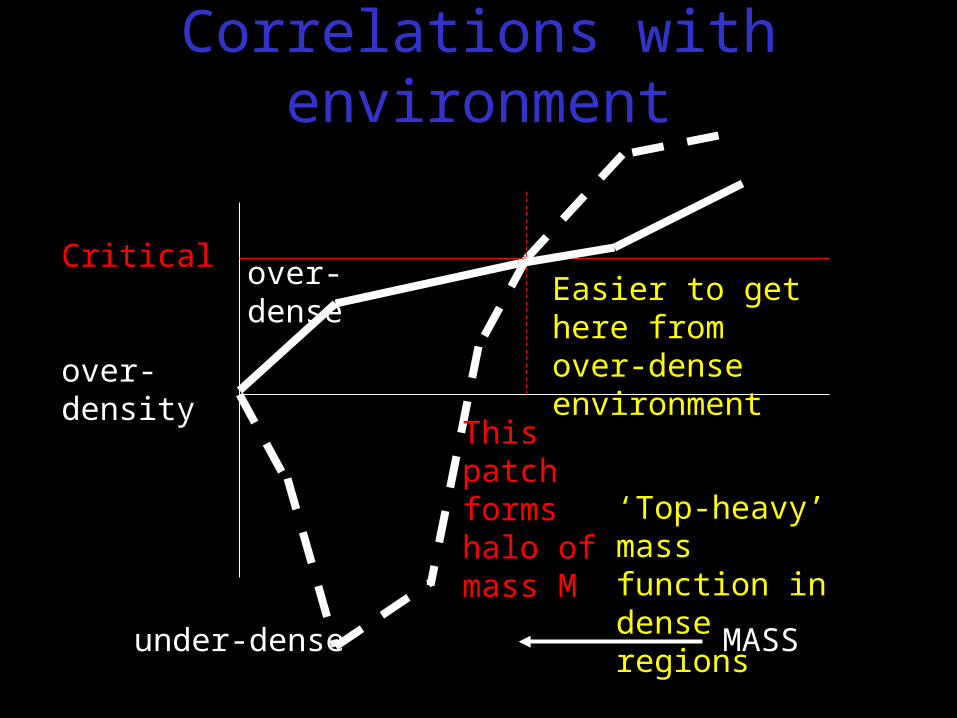
Critical

over-density

MASS

Easier to get here from over-dense environment

This patch forms halo of mass M

Correlations with environment

over-dense

under-dense

‘Top-heavy’ mass function in dense regions

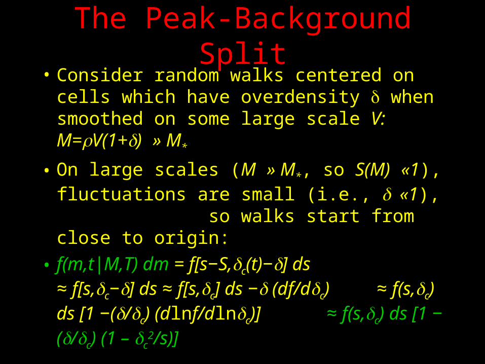
The Peak-Background Split• Consider random walks centered on cells

which have overdensity when smoothed on some large scale V: M=V(1+) » M*

• On large scales (M » M*, so S(M) «1), fluctuations are small (i.e., «1), so walks start from close to origin:

• f(m,t|M,T) dm = f[s−S,c(t)−] ds ≈ f[s,c−] ds ≈ f[s,c] ds − (df/dc) ≈ f(s,c) ds [1 −(/c) (dlnf/dlnc)] ≈ f(s,c) ds [1 −(/c) (1 – c

2/s)]

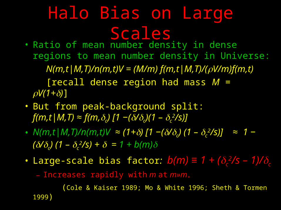
Halo Bias on Large Scales• Ratio of mean number density in dense regions to

mean number density in Universe:

N(m,t|M,T)/n(m,t)V = (M/m) f(m,t|M,T)/(V/m)f(m,t)

[recall dense region had mass M = V(1+)]• But from peak-background split: f(m,t|

M,T) ≈ f(m,c) [1 −(/c)(1 – c2/s)]

• N(m,t|M,T)/n(m,t)V ≈ (1+) [1 −(/c) (1 – c2/s)]

≈ 1 − (/c) (1 – c2/s) + = 1 + b(m)

• Large-scale bias factor: b(m) ≡ 1 + (c2/s – 1)/c

– Increases rapidly with m at m»m*

(Cole & Kaiser 1989; Mo & White 1996; Sheth & Tormen 1999)

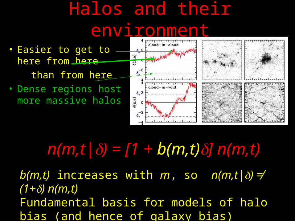
Halos and their environment

• Easier to get to here from here

than from here • Dense regions host

more massive halos

n(m,t|) = [1 + b(m,t)] n(m,t)

b(m,t) increases with m, so n(m,t|) ≠ (1+) n(m,t)Fundamental basis for models of halo bias (and hence of galaxy bias)

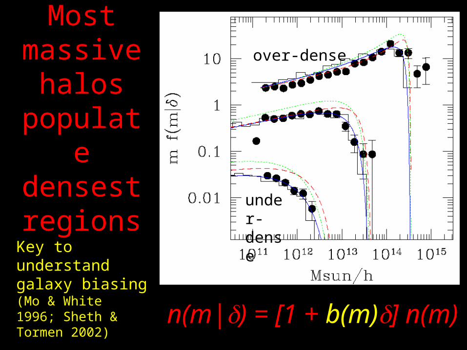
Most massive

halos populate densest regions

over-dense

under-dense

Key to understand galaxy biasing (Mo & White 1996; Sheth & Tormen 2002)

n(m|) = [1 + b(m)] n(m)

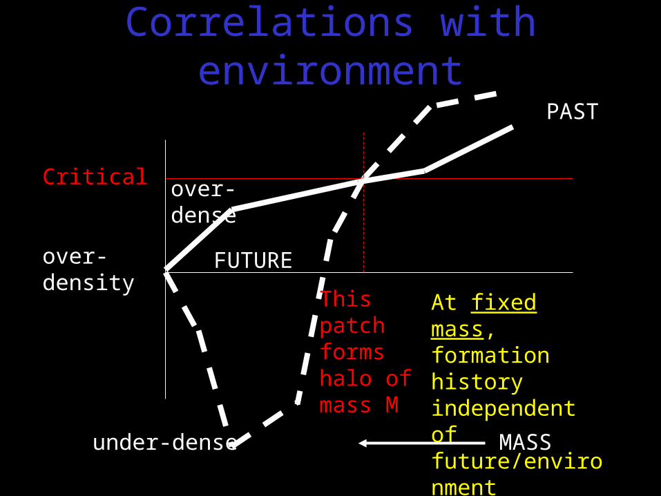
Critical

over-density

MASS

At fixed mass, formation history independent of future/environment

This patch forms halo of mass M

Correlations with environment

PAST

FUTURE

over-dense

under-dense

Environmental effects• In hierarchical models, close

connection between evolution and environment (dense region ~ dense universe ~ more evolved)

• Observed correlations with environment test hierarchical galaxy formation models

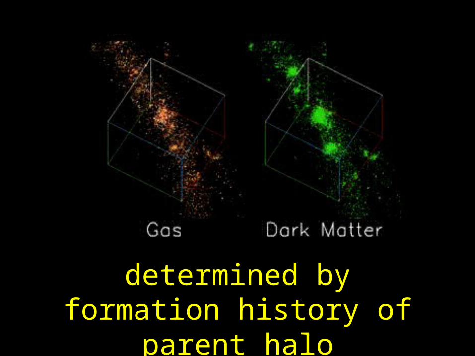
Gastrophysics determined by formation history of parent halo

Environmental effects• Gastrophysics determined by formation

history of parent halo

• All environmental trends come from fact that massive halos populate densest regions

THE HALO MODEL

Light is a biased tracer

Not all galaxies are fair tracers of dark matter;To use galaxies as probes of underlying dark matter distribution, must understand ‘bias’

How to describe different point processes which are all built from the same underlying distribution?

THE HALO MODEL

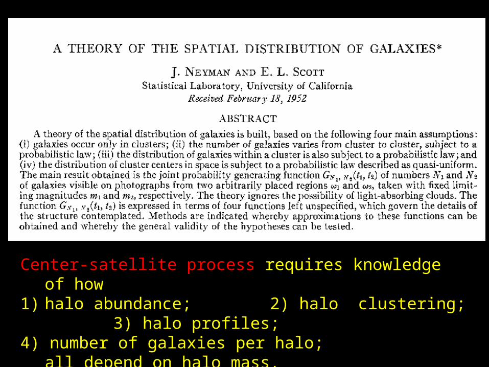
Center-satellite process requires knowledge of how 1) halo abundance; 2) halo clustering; 3) halo profiles; 4) number of galaxies per halo; all depend on halo mass.

(Revived, then discarded in 1970s by Peebles, McClelland & Silk)

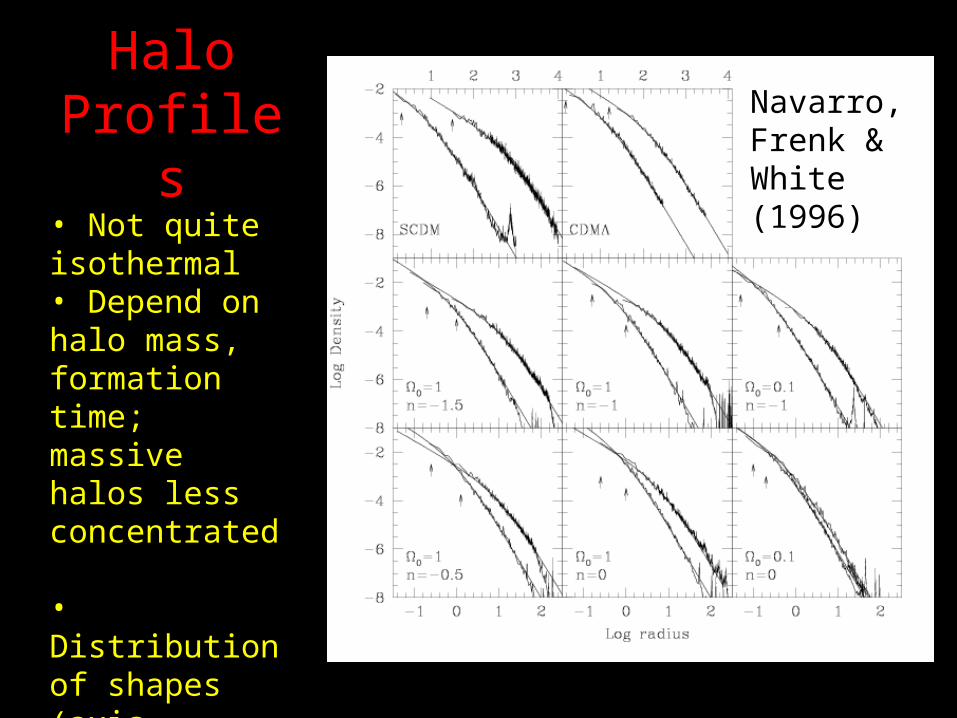
Halo Profiles

• Not quite isothermal • Depend on halo mass, formation time; massive halos less concentrated

• Distribution of shapes (axis-ratios) known (Jing & Suto 2001)

Navarro, Frenk & White (1996)

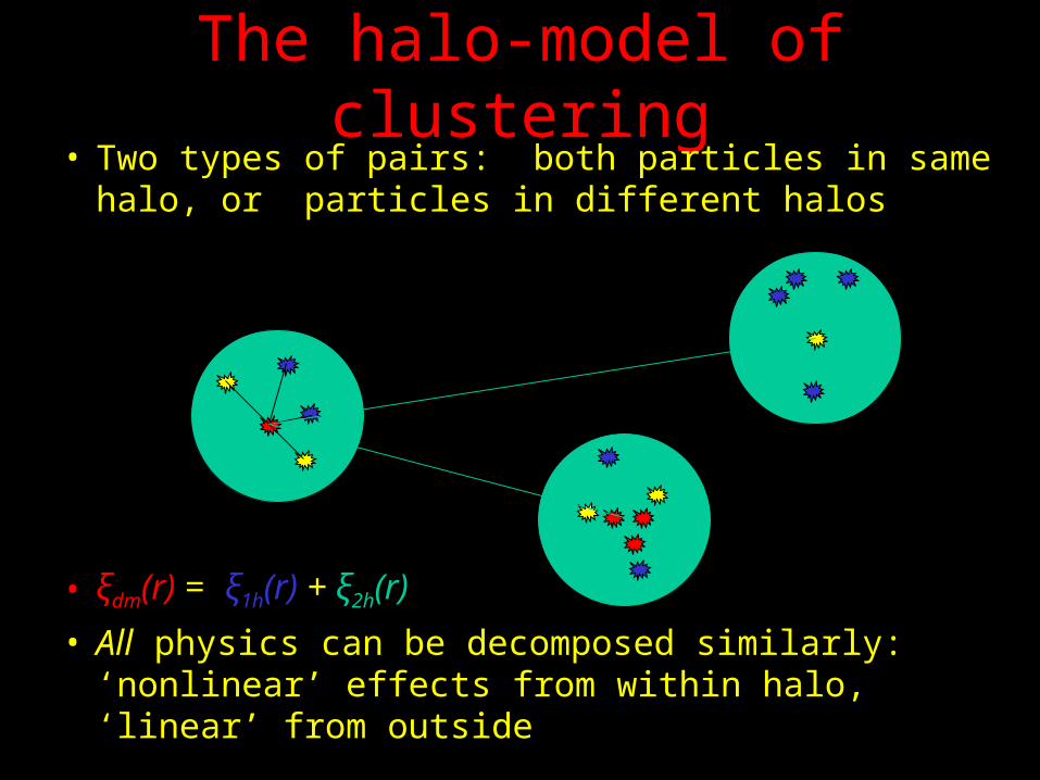
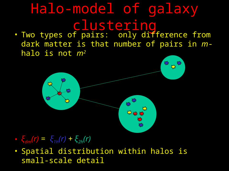
The halo-model of clustering• Two types of pairs: both particles in same halo, or

particles in different halos

• ξdm(r) = ξ1h(r) + ξ2h(r)

• All physics can be decomposed similarly: ‘nonlinear’ effects from within halo, ‘linear’ from outside

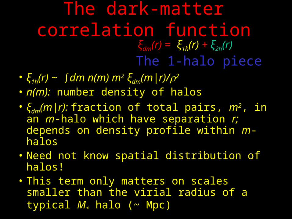
The dark-matter correlation function

ξdm(r) = ξ1h(r) + ξ2h(r)

The 1-halo piece• ξ1h(r) ~ ∫dm n(m) m2 ξdm(m|r)/2

• n(m): number density of halos• ξdm(m|r): fraction of total pairs, m2, in an m-

halo which have separation r; depends on density profile within m-halos

• Need not know spatial distribution of halos! • This term only matters on scales smaller than

the virial radius of a typical M* halo (~ Mpc)

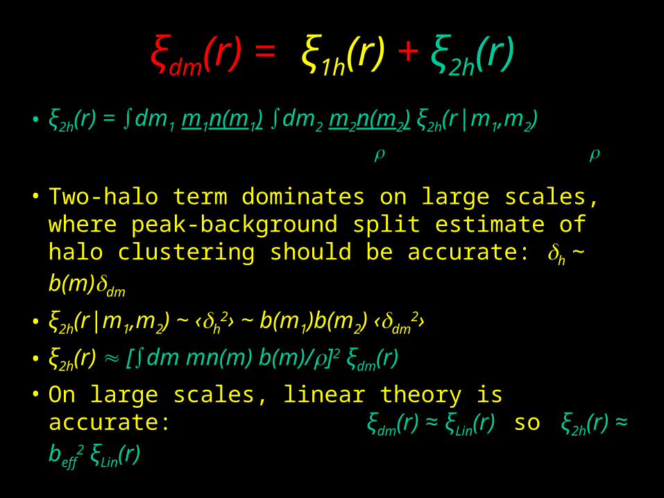
ξdm(r) = ξ1h(r) + ξ2h(r)

• ξ2h(r) = ∫dm1 m1n(m1) ∫dm2 m2n(m2) ξ2h(r|m1,m2)

• Two-halo term dominates on large scales, where peak-background split estimate of halo clustering should be accurate: h ~ b(m)dm

• ξ2h(r|m1,m2) ~ ‹h2› ~ b(m1)b(m2) ‹dm

2›

• ξ2h(r) ≈ [∫dm mn(m) b(m)/]2 ξdm(r)

• On large scales, linear theory is accurate: ξdm(r) ≈ ξLin(r) so ξ2h(r) ≈ beff

2 ξLin(r)

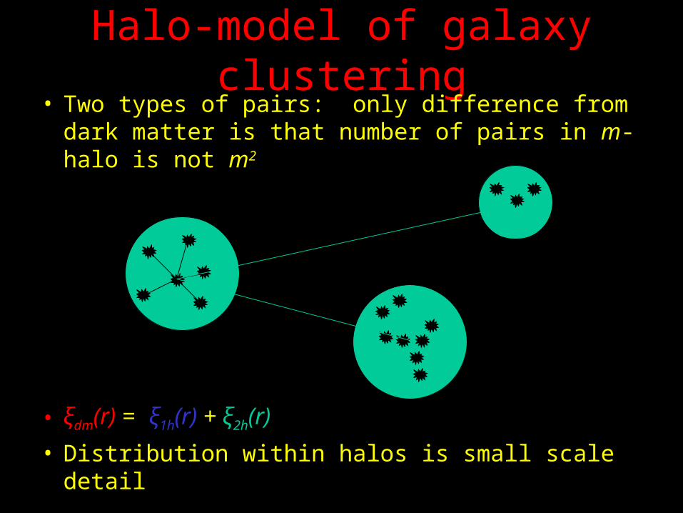
Halo-model of galaxy clustering• Two types of pairs: only difference from dark matter

is that number of pairs in m-halo is not m2

• ξdm(r) = ξ1h(r) + ξ2h(r)

• Distribution within halos is small scale detail

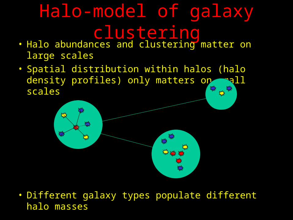
Halo-model of galaxy clustering• Halo abundances and clustering matter on large scales • Spatial distribution within halos (halo density

profiles) only matters on small scales

• Different galaxy types populate different halo masses

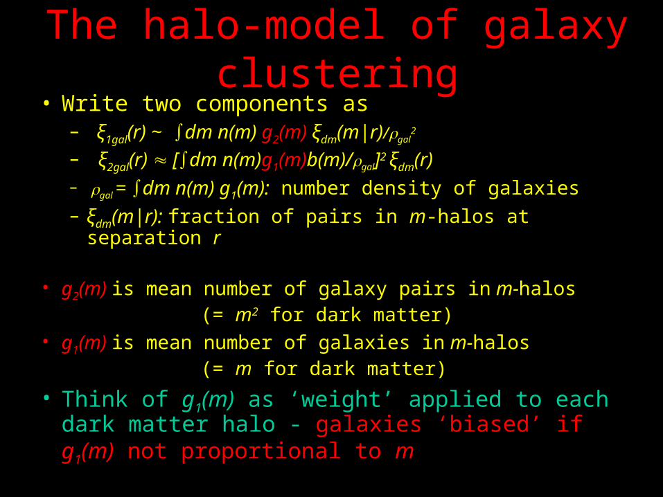
The halo-model of galaxy clustering• Write two components as

– ξ1gal(r) ~ ∫dm n(m) g2(m) ξdm(m|r)/gal2

– ξ2gal(r) ≈ [∫dm n(m)g1(m)b(m)/gal]2 ξdm(r)

– gal = ∫dm n(m) g1(m): number density of galaxies– ξdm(m|r): fraction of pairs in m-halos at separation r

• g2(m) is mean number of galaxy pairs in m-halos (= m2 for dark matter)• g1(m) is mean number of galaxies in m-halos (= m for dark matter)

• Think of g1(m) as ‘weight’ applied to each dark matter halo - galaxies ‘biased’ if g1(m) not proportional to m

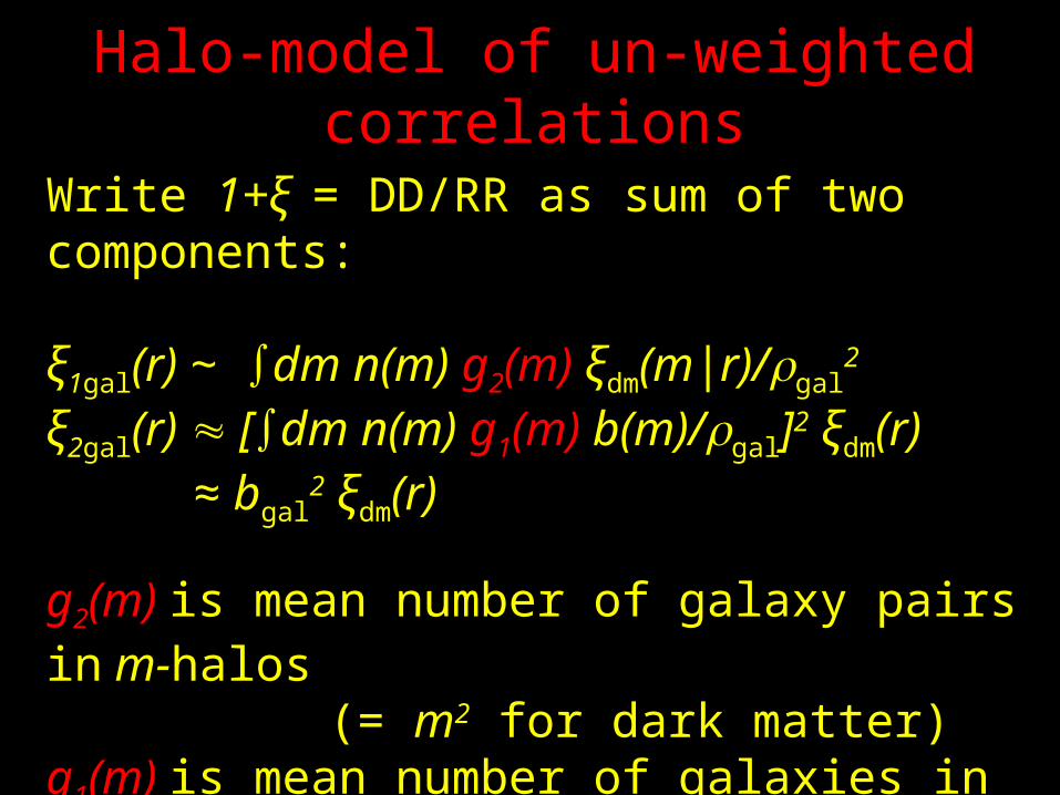
Halo-model of un-weighted correlations

Write 1+ξ = DD/RR as sum of two components:

ξ1gal(r) ~ ∫dm n(m) g2(m) ξdm(m|r)/gal2

ξ2gal(r) ≈ [∫dm n(m) g1(m) b(m)/gal]2 ξdm(r) ≈ bgal

2 ξdm(r)

g2(m) is mean number of galaxy pairs in m-halos (= m2 for dark matter)g1(m) is mean number of galaxies in m-halos (= m for dark matter)

Halo-model of galaxy clustering• Two types of pairs: only difference from dark matter

is that number of pairs in m-halo is not m2

• ξdm(r) = ξ1h(r) + ξ2h(r)

• Spatial distribution within halos is small-scale detail

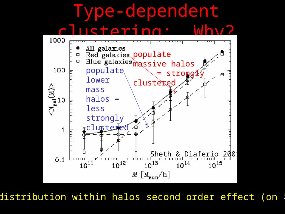
Type-dependent clustering: Why?

populate massive halos = strongly clustered

populate lower mass halos = less strongly clustered

Spatial distribution within halos second order effect (on >100 kpc)

Sheth & Diaferio 2001

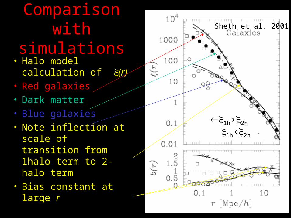
Comparison with simulations

• Halo model calculation of (r)

• Red galaxies• Dark matter• Blue galaxies• Note inflection at scale

of transition from 1halo term to 2-halo term

• Bias constant at large r

1h›2h

1h‹2h →

Sheth et al. 2001

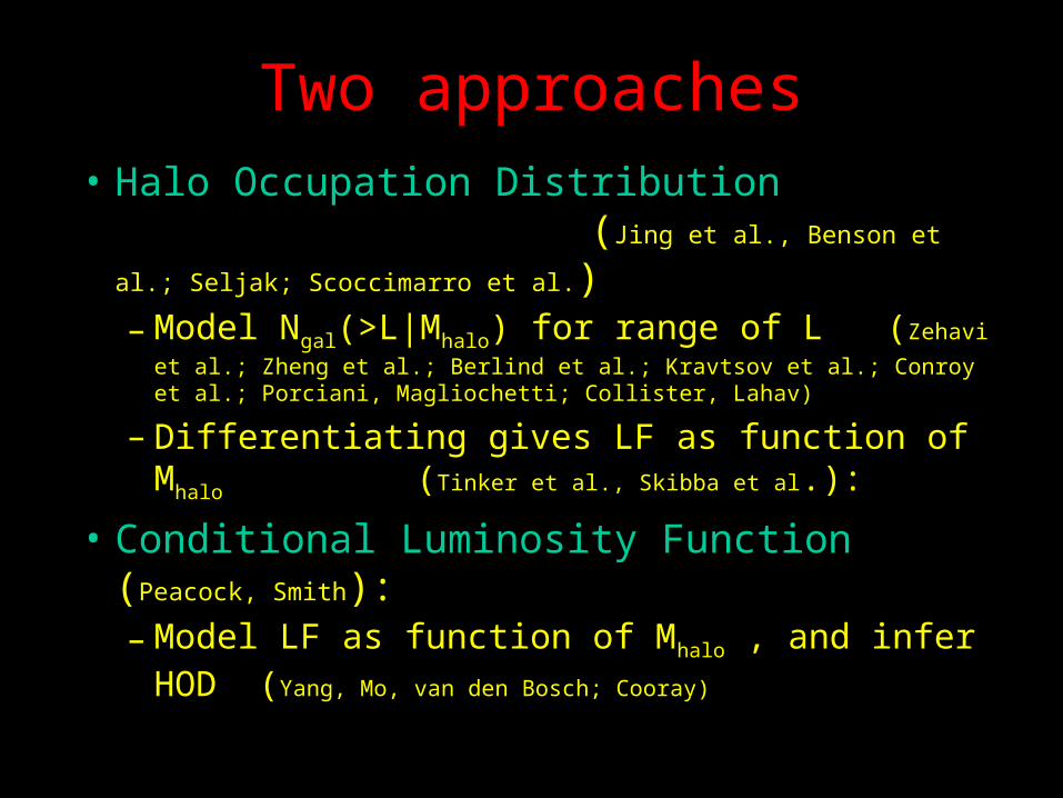
Two approaches• Halo Occupation Distribution

(Jing et al., Benson et al.; Seljak; Scoccimarro et al.)– Model Ngal(>L|Mhalo) for range of L (Zehavi et al.; Zheng et

al.; Berlind et al.; Kravtsov et al.; Conroy et al.; Porciani, Magliochetti; Collister, Lahav)

– Differentiating gives LF as function of Mhalo

(Tinker et al., Skibba et al.):

• Conditional Luminosity Function (Peacock, Smith): – Model LF as function of Mhalo , and infer HOD (Yang,

Mo, van den Bosch; Cooray)

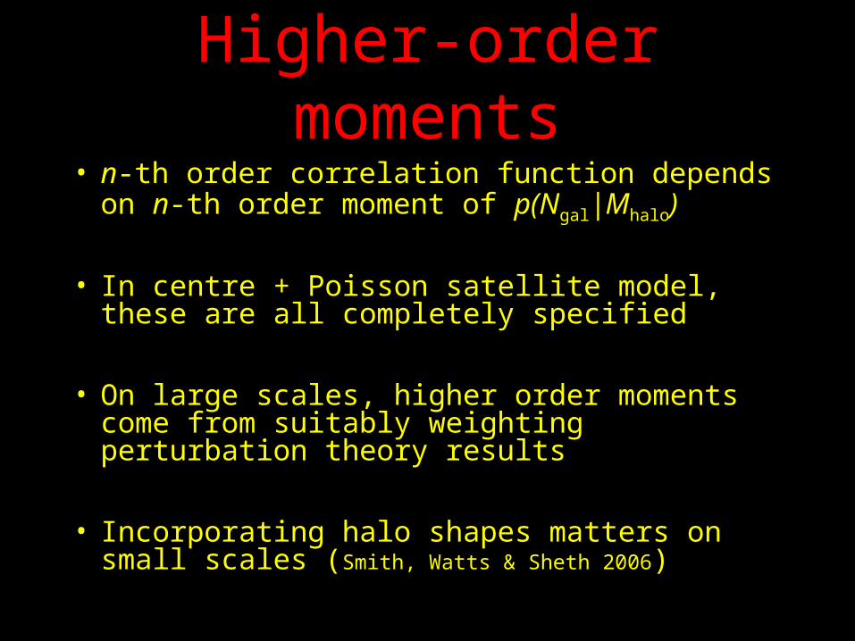
Higher-order moments• n-th order correlation function depends on n-th

order moment of p(Ngal|Mhalo)

• In centre + Poisson satellite model, these are all completely specified

• On large scales, higher order moments come from suitably weighting perturbation theory results

• Incorporating halo shapes matters on small scales (Smith, Watts & Sheth 2006)

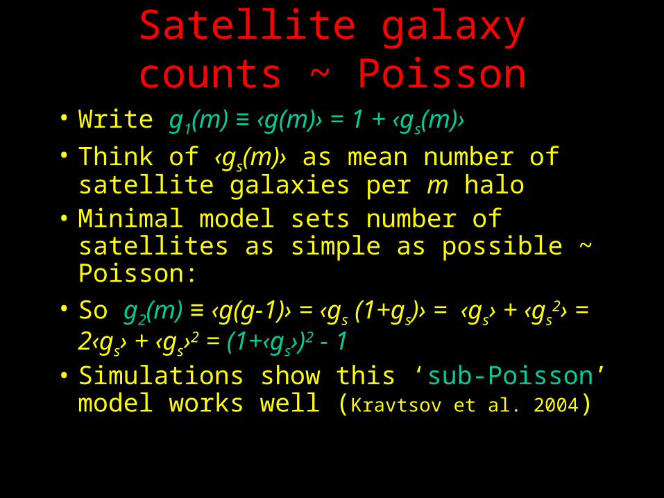
Satellite galaxy counts ~ Poisson

• Write g1(m) ≡ ‹g(m)› = 1 + ‹gs(m)›• Think of ‹gs(m)› as mean number of satellite

galaxies per m halo• Minimal model sets number of satellites as

simple as possible ~ Poisson: • So g2(m) ≡ ‹g(g-1)› = ‹gs (1+gs)› = ‹gs› +

‹gs2› = 2‹gs› + ‹gs›2 = (1+‹gs›)2 - 1

• Simulations show this ‘sub-Poisson’ model works well (Kravtsov et al. 2004)

Halo Substructure

• Halo substructure = galaxies is good model (Klypin et al. 1999; Kravtsov et al. 2005)

• Agrees with semi-analytic models and SPH (Berlind et al. 2004; Zheng et al. 2005; Croton et al. 2006)

• Setting n(>L) = n(>Vcirc) works well for all clustering analyses to date, including z~3 (Conroy et al. 2006)

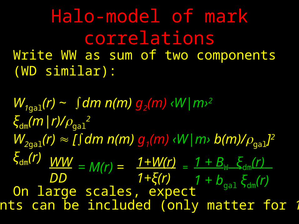
Halo-model of mark correlations

Write WW as sum of two components (WD similar):

W1gal(r) ~ ∫dm n(m) g2(m) ‹W|m›2 ξdm(m|r)/gal2

W2gal(r) ≈ [∫dm n(m) g1(m) ‹W|m› b(m)/gal]2 ξdm(r)

On large scales, expect

= M(r) = 1+W(r)1+ξ(r)

= 1 + BW ξdm(r) 1 + bgal ξdm(r)

WWDD

Gradients can be included (only matter for 1h term)

Note assumption!

• Whereas mark may correlate with halo mass, there is no additional correlation between mark and environment

• Greatly simplifies galaxy formation models and interpretation of galaxy clustering: – Some semi-analytic galaxy formation models

assume this explicitly (when use semi-analytic merger trees rather than trees from simulation)

Assumptions (to test)• Halo profiles depend on mass, not

environment• Galaxy properties, so p(Ngal|L,m), and so

g1(m) and g2(m), depend on halo mass, not environment

• All environmental dependence comes from correlation between halo mass and environment:

n(m|) = [1+b(m)n(m)– Mass function ‘top-heavy’ in dense regions

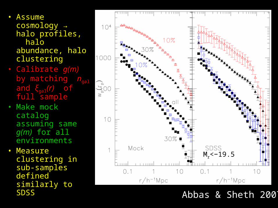
• Assume cosmology → halo profiles, halo abundance, halo clustering

• Calibrate g(m) by matching ngal and ξgal(r) of full sample

• Make mock catalog assuming same g(m) for all environments

• Measure clustering in sub-samples defined similarly to SDSS

SDSS

Abbas & Sheth 2007

Mr<−19.5

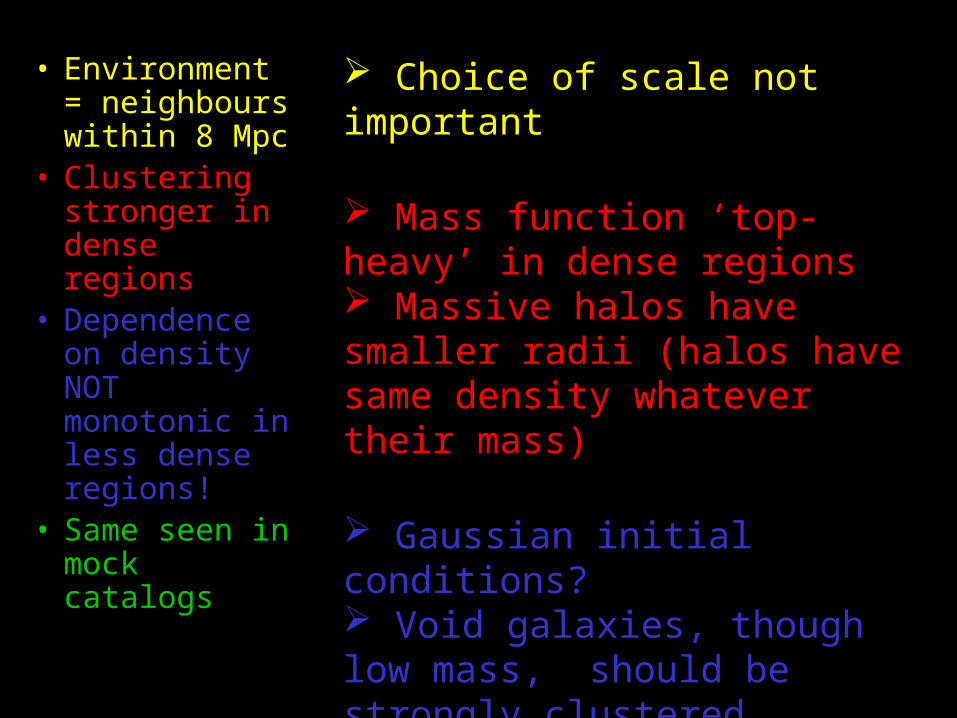
• Environment = neighbours within 8 Mpc

• Clustering stronger in dense regions

• Dependence on density NOT monotonic in less dense regions!

• Same seen in mock catalogs

SDSS

Choice of scale not important

Mass function ‘top-heavy’ in dense regions Massive halos have smaller radii (halos have same density whatever their mass)

Gaussian initial conditions? Void galaxies, though low mass, should be strongly clustered

Little room for additional (e.g. assembly bias) environmental effects

Halo Model is simplistic …

• Nonlinear physics on small scales from virial theorem

• Linear perturbation theory on scales larger than virial radius (exploits 20 years of hard work between 1970-1990)

…but quite accurate!

Thus, one can …

• Model both real and redshift space observations

• Model clustering of thermal SZ effect as a weight proportional to pressure, applied to halos/clusters

• Model clustering of kinetic SZ signal as a weight, proportional to halo/cluster momentum

• Model weak gravitational galaxy-galaxy lensing as cross-correlation between galaxies and mass in halos

• (see review article Cooray & Sheth 2002)

• Number density and clustering as function of luminosity now measured in 2dF,SDSS

• Assuming there are NO large scale environmental effects, halo model provides estimates of luminosity distribution as function of halo mass (interesting, relatively unexplored connection to cluster LFs)

• Suggests BCGs are special population (another interesting, unexplored connection to clusters!)

The Holy Grail

Halo model provides natural framework within which to discuss, interpret most measures of clustering; it is the natural language of galaxy ‘bias’

The Halo Grail

The Cup!

India Cricket World Champions

Cracks in the standard model• Sheth &Tormen (2004) measure correlation

between formation time and environment:– At fixed mass, close pairs form earlier

– Point out relevance to halo model description

– Measurement repeated and confirmed by Gao et al. (2005), Harker et al. (2006), Wechsler et al. (2006)

• Early formation more clustered (even at fixed mass) at low masses

• Does this matter for surveys which use clustering of (primarily) luminous galaxies for cosmology (Abbas & Sheth 2005, 2006; Croton et al. 2006)?

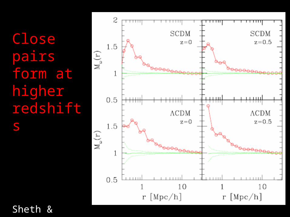
Close pairs form at higher redshifts

Sheth & Tormen 2004

A direct test of the importance of this effect using the SDSS

Based on – Abbas & Sheth (2005): Clustering as

function of environment (theory)– Abbas & Sheth (2006): Environmental

dependence of clustering in the SDSS– Abbas & Sheth (2007): Strong clustering

of under-dense regions

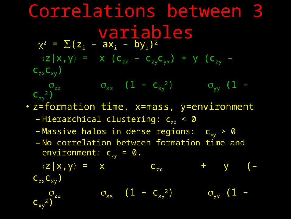
Correlations between 3 variables• = ∑(zi – axi – byi)2

z|x,y = x (czx – czycyx) + y (czy – czxcxy)

_____ __ _________ __ _________

zz xx (1 – cxy2) yy (1 – cxy

2) • z=formation time, x=mass, y=environment

– Hierarchical clustering: czx < 0– Massive halos in dense regions: cxy > 0– No correlation between formation time and

environment: czy = 0.

z|x,y = x czx + y (– czxcxy)

_____ __ _________ __ _________

zz xx (1 – cxy2) yy (1 – cxy

2)