The performance of a static coal classifier and its ... · 4.2 Scaled model of vertical spindle...

i

The performance of a static coal classifier and its

controlling parameters

Thesis submitted to the University of Leicester for the

degree of Doctor of Philosophy

By Jamiu Lanre Afolabi

January 2012

ii

Abstract

In power generation from solid fuel such as coal-fired power plants, combustion

efficiency can be monitored by the Loss on Ignition (LOI) of the pulverised fuel. It is

the role of the pulveriser-classifier combination to ensure pulverised fuel delivered to

the burners is within the specified limits of fineness and mass flow deviation required to

keep the LOI at an acceptable level. Government imposed limits on emissions have

spurred many coal fired power plants to convert to the use of Low NOx Burners. To

maintain good LOI or combustion efficiency, the limits of fineness and mass flow

deviation or inter-outlet fuel distribution have become narrower. A lot of existing

pulveriser units cannot operate effectively within these limits hence retrofits of short

term solutions such as orifice balancing and classifier maintenance has been applied.

The work performed in this thesis relates to an investigation into coal classifier devices

that function to control fineness and inter pipe balancing upstream of the burner and

downstream of the pulverisers.

A cold flow model of a static classifier was developed to investigate the flow

characteristics so that design optimisations can be made. Dynamic similarity was

achieved by designing a 1/3 scale model with air as the continuous phase and glass

cenospheres of a similar size distribution as pulverised fuel, to simulate the coal dust.

The rig was operated in positive pressure with air at room temperature and discharge to

atmosphere. The Stokes number similarity (0.11-prototype vs. 0.08-model) was the

most important dimensionless parameter to conserve as Reynolds number becomes

independent of separation efficiency and pressure drop at high industrial values such as

2 x 104 (Hoffman, 2008). Air-fuel ratio was also compromised and an assumption of

dilute flow was made to qualify this. However, the effect of air fuel ratio was

ascertained by its inclusion as an experimental variable. Experiments were conducted at

air flow rates of 1.41-1.71kg/s and air fuel ratios of 4.8-10 with classifier vane angle

adjustment (30°- 60°) and inlet swirl numbers (S) of 0.49 – 1. Radial profiles of

tangential, axial and radial velocity were obtained at several cross sections to determine

the airflow pattern and establish links with the separation performance and outlet flow

balance. Results show a proportional relationship between cone vane angle and cut size

or particle fineness. Models can be derived from the data so that reliable predictions of

fineness and outlet fuel balance can be used in power stations and replace simplistic and

process simulator models that fail to correctly predict performance. It was found that

swirl intensity is a more significant parameter in obtaining a balanced flow at the

classifier outlets than uniform air flow distribution in the mill. However the latter is

important in obtaining high grade efficiencies and cut size. The study concludes that the

static classifier can be further improved and retrofit-able solutions can be applied to

problems of outlet flow imbalance and poor fineness at the mill outlets.

iii

Acknowledgements

This thesis is dedicated to my dear parents Lola and Bola Afolabi of whom I appreciate

their support in every aspect of life. Special thanks to Prof S.B Afolabi for the financial

assistance without which this opportunity would not be possible.

I wish to thank:

Professor A. Aroussi who created and supervised the project in its early stages.

Greenbank Terotech for their financial support, rig development and industrial input.

Alan Wale, the lead technician in the fabrication of the experimental facility.

Paul Williams, the instrumentation and safety officer for his valuable input.

All of the technicians at the University of Leicester departmental workshop especially

Dipak Raval, Simon Millward and Ian Bromley.

Neetin Lad and my colleagues within the Aroussi team for the useful discussions and

debates that inspire creativity.

My awesome family and friends.

And finally my soulmate Aisha, who has been a shining star during this whole process.

iv

Contents

Chapter 1: Introduction…………………………………………………………………..1

1.1 Background ........................................................................................................ 1

1.2 The classifier problem ........................................................................................ 3

1.3 Project aims ........................................................................................................ 4

1.4 Thesis structure .................................................................................................. 5

Chapter 2 : Literature Review …………………………………………………………...7

2.1 Introduction ........................................................................................................ 7

2.2 Coal comminution in pulverisers ....................................................................... 7

2.2.1 Types of pulverisers .................................................................................... 9

2.3 Coal classification ............................................................................................ 12

2.3.1 Classifier performance .............................................................................. 12

2.3.2 Types of coal classifiers ............................................................................ 13

2.3.3 Classifier flow field .................................................................................. 16

2.3.4 Particle Motion ......................................................................................... 18

2.3.5 Multiphase classifier studies ..................................................................... 19

2.4 Summary .......................................................................................................... 21

Chapter 3 : Characterisation of the Preliminary Classifier Model.…………………….22

3.1 Introduction .................................................................................................... 22

3.2 Preliminary model description ....................................................................... 23

3.2.1 Experimental setup and procedure .............................................................. 24

3.3 Flow measurement results in preliminary model ........................................... 27

3.3.1 Inlet velocity effect on the flow field .......................................................... 27

3.3.2 Vane angle effect on outlet flow region ...................................................... 29

3.3.3 Summary of results ..................................................................................... 30

3.4 Computational fluid dynamic study ............................................................... 31

3.4.1 CFD geometry development ....................................................................... 31

3.4.2 Mesh independency .................................................................................... 32

3.4.3 Flow governing equations ........................................................................... 33

3.4.4 Turbulence models ...................................................................................... 34

3.4.4.1 Realizable k-ε ..................................................................................... 34

3.4.4.2 The RNG k-ε ....................................................................................... 35

3.4.4.3 The RSM model .................................................................................. 36

3.4.5 Multiphase simulation methodology .......................................................... 37

v

3.4.5.1 Trajectory Modelling ......................................................................... 38

3.4.5.2 Turbulence effect on the interactions between the solid and gas

phases…… .............................................................................................................. 39

3.4.6 Predicted air flow pattern ........................................................................... 39

3.4.6.1 Tangential Velocity ............................................................................ 40

3.4.6.2 Turbulence models.............................................................................. 43

3.4.7 Outlet design and performance predictions ................................................ 44

3.4.7.1 CFD input parameters ......................................................................... 45

3.4.7.1 Classification performance and grade efficiency ............................... 45

3.4.7.2 Inlet velocity and cut size ................................................................... 46

3.4.7.3 Particle trajectory visualisation........................................................... 46

3.4.8 Conclusions of the initial model CFD study ............................................... 49

Chapter 4 : Advanced Classifier Model Design and Instrumentation………………….51

4.1 Introduction ..................................................................................................... 51

4.2 Scaled model of vertical spindle mill classifier .............................................. 52

4.2.1 Static port ring model variations ................................................................. 54

4.3 Dimensional analysis and similarity ............................................................... 56

4.3.1 Separation efficiency 57

4.3.2 Pressure drop ............................................................................................... 60

4.3.3 Experimental model limitations .................................................................. 61

4.4 Experimental facility ....................................................................................... 62

4.4.1 Air mover .................................................................................................... 64

4.4.2 Conveyed Material ...................................................................................... 66

4.4.3 Particle feeding device ................................................................................ 68

4.4.4 Flow measurement and instrumentation ..................................................... 70

4.4.4.1 5- hole pressure probe description .................................................. 71

4.4.4.1 Probe calibration ............................................................................. 71

4.4.4.2 Calibration results and data reduction ............................................ 74

4.4.4.3 Resolving flow angles and velocity ................................................ 75

4.4.4.4 Error and uncertainty in calibration ................................................ 76

4.4.5 Cyclone separator ....................................................................................... 78

4.4.5.1 Cyclone design ................................................................................ 78

4.4.5.2 Pressure drop predictions ................................................................ 80

4.4.5.3 Separation efficiency predictions .................................................... 81

4.5 Particle size analysis ....................................................................................... 86

4.5.1 Sieve Analysis ............................................................................................. 86

4.5.2 Image analysis ............................................................................................. 86

vi

4.5.3 Particle measurement .................................................................................. 87

4.6 Conclusions………………………………………………………………….... 90

Chapter 5 : Classifier Air Flow Characterisation………………………………………92

5.1 Introduction ..................................................................................................... 92

5.2 Swirl number ................................................................................................... 92

5.3 Airflow distribution ........................................................................................ 95

5.3.1 Circumferential velocity profiles .............................................................. 96

5.3.2 Inter-outlet mass flow balance .................................................................. 99

5.4 Classifier flow pattern ................................................................................... 100

5.4.1 Effect of inlet configuration .................................................................... 104

5.4.2 Annular flow ........................................................................................... 109

5.4.2.1 Tangential velocity in the annular region ......................................... 109

5.4.2.2 Axial velocity in annular region ....................................................... 113

5.4.2.3 Radial velocity in annular region ...................................................... 117

5.4.3 Separation zone flow pattern .................................................................. 120

5.4.3.1 Tangential velocity in the main separation zone .............................. 120

5.4.3.2 Axial velocity in the main separation zone ...................................... 124

5.4.3.3 Radial velocity in the main separation zone ..................................... 126

5.5 Conclusions ................................................................................................... 128

Chapter 6 : Powder Experiments and Classifier Performance Results………………..121

6.1 Introduction ................................................................................................... 121

6.2 Test procedure ............................................................................................... 121

6.2.1 Experimental test parameters ................................................................ 122

6.3 Particle mass balance .................................................................................... 126

6.4 Size distribution of recovered particles ........................................................ 126

6.4.1 Outlet particle cumulative undersize distributions ............................... 127

6.4.2 Reject particulate cumulative undersize distributions .......................... 128

6.5 Overall collection efficiency ......................................................................... 130

6.5.1 Effect of swirl intensity on collection efficiency .................................. 130

6.6 Grade efficiency and cut size ........................................................................ 131

6.6.1 Effect of swirl intensity on grade efficiency and cut size ..................... 131

6.6.2 Effect of cone vane angle ...................................................................... 133

6.6.3 Effect of inlet velocity on grade efficiency and cut size ....................... 135

6.6.4 Effect of solid loading on grade efficiency and cut size ....................... 136

6.7 Outlet mass balance of solids ........................................................................ 137

6.7.1 Effect of inlet design on particle mass balance ..................................... 139

vii

6.7.2 Effect of cone vane angle on particle mass balance ............................. 141

6.7.3 Effect of inlet velocity and solids loading on particle mass balance .... 142

6.8 Conclusions ................................................................................................... 144

Chapter 7 : Conclusions…………………………………………………………….....145

7.1 Overview ........................................................................................................ 145

7.2 Concluding remarks ....................................................................................... 146

7.3 Future work .................................................................................................... 148

Appendix A : Dimensional Analysis ………………………………………………...150

Appendix B : Full radial profiles of tangential velocity………………………………152

Appendix C : Radial profiles of pressure in the separation zone…………………......153

Appendix D : Data acquisition programme…………………………………………...156

Appendix E: Microscopy particle sizing calculations………………………………...157

Appendix F: Raw particle data from tests…………………………………………….162

Appendix G : Dry Sieving experimental procedure…………………………………..163

Bibliography…………………………………………………………………………..164

viii

List of Figures

Figure 1.1 Stratified furnace O2 profile as a result of fuel imbalance (Storm, 2009) ....... 3

Figure 2.1: Low speed tube ball mill, also known as ‘tumbling mill’, (Foster Wheeler,

Inc)…. 10

Figure 2.2: A Babcock & Wilcox E&L Vertical spindle mill. Maximum throughput

23tn/hr, (Babcock&Wilcox). ........................................................................................... 10

Figure 2.3: Hammer mill pulverisers used in coal fired power plants (Qingsheng and

Stodden, 2006). ............................................................................................................... 11

Figure 2.4: Centrifugal separation zones: (a) centrifugal counter-flow, (b) centrifugal

cross-flow (Shapiro and Galperin, 2005). ....................................................................... 14

Figure 2.5:Static and dynamic classifier separation principles. (a) Static classifier, (b)

dynamic classifier. .......................................................................................................... 15

Figure 2.6: Two commercial centrifugal classifiers. (a) Static classifier (Foster wheeler

MBF design) (b) dynamic classifier (Babcock&Wilcox design). ................................... 16

Figure 2.7: Sketch showing the two ideal vortex flows and the tangential velocity

distribution of a real vortex. ............................................................................................ 17

Figure 3.1: Above: model design and component list. Below: annotated section view of

the model. ........................................................................................................................ 23

Figure 3.2: Experimental setup of the preliminary model (LHS). Outlet assembly and

internal components in detail (RHS). ............................................................................. 25

Figure 3.3: Front view cross section of classifier showing measurement locations and

flow schematic. ............................................................................................................... 26

Figure 3.4: (a) Mean tangential velocity profile at position A. (b) Mean tangential

velocity profile at position B. ......................................................................................... 28

Figure 3.5: (a) Mean tangential velocity profile at position C. (b) Mean tangential

velocity profile at position D. ......................................................................................... 28

Figure 3.6: Cone Vane Angle (CVA) reference position showing the view plane. ....... 29

Figure 3.7: Normalised mean tangential velocity profiles at position C for inlet

velocities (a) 10m/s and (b) 19m/s, at two different vane angles. .................................. 30

Figure 3.8: Normalised mean tangential velocity profiles at position D for inlet

velocities (a) 10m/s and (b) 19m/s at two different vane angles. ................................... 30

ix

Figure 3.9: Model cross section highlighting the high density mesh regions of the cone

wall, vanes and outlet structure ....................................................................................... 32

Figure 3.10: Numerical and experimental Vθ/Vin radial profiles at axial positions (a) A

and (b) B. Vin = 10ms-1

................................................................................................... 40

Figure 3.11: Numerical and experimental Vθ/Vin radial profiles at axial positions (a) C

and (b) D. Vin = 10ms-1

................................................................................................... 40

Figure 3.12: Numerical and experimental Vθ/Vin radial profiles at axial positions (a) A

and (b) B. Vin = 19ms-1

................................................................................................... 41

Figure 3.13: Numerical and experimental Vθ/Vin radial profiles at axial positions (a) C

and (b) D. Vin = 19ms-1

................................................................................................... 41

Figure 3.14: Characterised flow regions and their locations within classifier model.

Outlet region (OR), Core region (CR), Outer cone region (OCR) and Annular region

(AR) ................................................................................................................................ 43

Figure 3.15: Section view of model A (LHS) and model B (RHS) illustrating the

differences in design ....................................................................................................... 44

Figure 3.16: Overall efficiency variation with inlet velocity. A linear fit is shown for the

two points investigated ................................................................................................... 47

Figure 3.17: GEC comparison between geometries at AFR=4.8:1 and Vin =19m/s

showing the difference in X75 ......................................................................................... 47

Figure 3.18: GEC comparison between geometries at AFR=4.8:1 and Vin =30m/s

showing the difference in X7 .......................................................................................... 47

Figure 3.19: Fine particle trajectories for a single injection in geometries A and B

respectively, coloured by the particle residence time. .................................................... 48

Figure 3.20: Coarse particle trajectories for a single injection in geometries A and B

respectively, coloured by the particle residence time……………………………. 48

Figure 4.1: Cut away section view of the benchmark advanced classifier model,

numbered by its components listed in Table 4.1. ........................................................... 52

Figure 4.2: (a) 45° and (b) 30° static port ring models (SPR). ....................................... 54

Figure 4.3: Benchmark classifier model (TIC) without static port ring, showing

component dimensions in mm. ....................................................................................... 55

Figure 4.4: Static port ring (SPR) classifier model, showing section view and

dimensions in mm. .......................................................................................................... 55

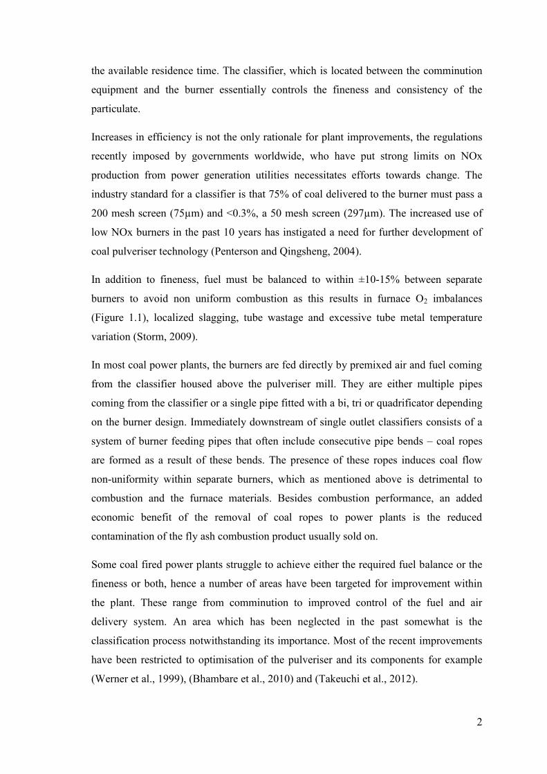
Figure 4.5: Experimental setup for classifier model ....................................................... 64

x

Figure 4.6: Images of the experimental facility (LHS) and a view of the outlet section

(top right) and inside the classifier (bottom right). ......................................................... 65

Figure 4.7: Inlet velocity profiles for various air mass flow rates ........................... 66

Figure 4.8: Motor frequency setting as a function of average inlet velocity. ................. 66

Figure 4.9: Microscopic image of the unprocessed feed fillite. ...................................... 67

Figure 4.10: Cumulative size distribution (CSD) of feed fillite. A comparison of

measured size distributions using image size analysis and standard dry sieving methods.

........................................................................................................................................ 67

Figure 4.11: Generic drop-through rotary valve (Mills, 2004). ...................................... 69

Figure 4.12: Scanning electron microscope image of a powder sample collected from

the cyclone hopper. Particles are generally intact. .......................................................... 69

Figure 4.13: Rotary valve calibration chart .................................................................... 70

Figure 4.14: 5-hole pressure probe used in the aerodynamic characterisation of the

classifier scale model. ..................................................................................................... 72

Figure 4.15: Probe calibration mechanism. The horizontal and vertical position is

adjusted at each angle to re-align the probe centrally, via the traverse rail and mount

shaft respectively. ........................................................................................................... 73

Figure 4.16: Calibration data showing the dependence of upon ......... 77

Figure 4.17: Calibration data showing the dependence of upon ......... 77

Figure 4.18: Calibration data showing the dependence of upon . ............. 77

Figure 4.19: Separation mechanism of a cyclone separator (Mills, 2004). .................... 78

Figure 4.20: Performance curves for typical cyclone separators. ................................... 79

Figure 4.21: Schematic of a Tengbergen B cyclone showing the dimensional notation

used herein (see table 4.5) ............................................................................................... 79

Figure 4.22: Plan view of a typical cylinder- on-cone cyclone showing additional

parameters required to calculate cyclone cut size (Hoffman, 2008). .............................. 83

Figure 4.23: Predicted grade efficiency of the Tengbergen cyclone used in the classifier

experiments. .................................................................................................................... 85

Figure 4.24: From top to bottom, and left to right; SEM images of a typical coarse

sample from the classifier at 80x 120x, 200x and 350x magnification. Particle counts in

each image are based on the requirement of a resulting standard error of less than 2% 89

xi

Figure 5.1: Cross sectional profiles of the tangential and axial momentum fluxes at near

inlet location for the TIC inlet configuration at normalised axial location y/Dc=0.45. . 94

Figure 5.2: Cross sectional profiles of the tangential and axial momentum fluxes at near

inlet location for the SPR30 inlet configuration at normalised axial location y/Dc=0.45.

........................................................................................................................................ 94

Figure 5.3: Cross sectional profiles of the tangential and axial momentum plots at near

inlet location for the SPR45 inlet configuration at normalised axial location y/Dc=0.45.

........................................................................................................................................ 94

Figure 5.4: Location of the angular reference points. Measurement pitch diameter on the

cylindrical surface in which the measurements apply. ................................................... 96

Figure 5.5: Circumferential variation of the normalised mean velocity for different inlet

designs. The standard deviations about the average values in the profile are shown for

both models. Measurements are taken at (a) y=550mm and (b) y=1250mm. Inlet

velocity Vin = 14.4m/s. .................................................................................................... 98

Figure 5.6: Circumferential variation of the normalised mean velocity for 45 and 60

degree cone vane angles- (a) and (b) respectively. Effect of inlet velocity is shown for

measurements in the TIC inlet design at axial position Y = 550mm (y/Dc =0.46) ........ 98

Figure 5.7: Circumferential variation of the normalised mean velocity for 45 and 60

degree cone vane angles- (a) and (b) respectively. Effect of inlet velocity is shown for

measurements in the TIC inlet design at axial position Y = 1250mm (y/Dc =1.04) ...... 98

Figure 5.8: Schematic of the classifier outlet configuration with numbered outlet pipes.

........................................................................................................................................ 99

Figure 5.9: Mass flow deviation (%) from the mean of the air phase as a function of

inlet mass flow rate. (a) ζ=30°, (b) , ζ=45°and (c) ζ=60° cone vane angle settings in the

TIC inlet design. ........................................................................................................... 101

Figure 5.10: Standard deviation of the average air mass flow rate between the outlet

pipes at different inlet flow rates (0.79, 1.07, 1.4, and 1.729kg/m3) for the TIC inlet.

Each curve represents a cone vane angle ( ) setting. ................................................... 101



SPR30 inlet design. ...................................................................................................... 102

Figure 5.12: Standard deviation of the mean air mass flow rate between the outlet pipes

at different inlet mass flow rates (0.79, 1.07, 1.4, and 1.729kg/m3) for SPR30. Each

curve represents a cone vane angle ( ) setting. ............................................................ 102

xii



SPR45 inlet design. ....................................................................................................... 103

Figure 5.14: Standard deviation of the mean air mass flow rate between the outlet pipes

at different inlet mass flow rates (0.79, 1.07, 1.4, and 1.729kg/m3) for SPR45. Each

curve represents a cone vane angle ( ) setting. ............................................................ 103

Figure 5.15: (a) Measurement planes. Arrows indicate plane of the results presented in

this section (b) Axial stations where measurements are taken ..................................... 104

Figure 5.16: Tangential velocity profiles of TIC, SPR30 and SPR45 inlet geometries at

normalised axial position y/Dc = 0.84 and cone vane angle = 45°. The dashed lines at

0.063, 0.163 and 0.307 represent the walls of the central chute, vortex finder, and the

cone respectively, where Vin = 14.4 m/s. ..................................................................... 105

Figure 5.17: Radial profiles of (a) tangential velocity (b) axial velocity, and (c) radial

velocity. The dashed lines at 0.063 and 0.267 represent the wall of the central chute and

cone respectively. Measurements are taken at y/Dc = 0.73 at a cone vane angle = 45°

and Vin = 14.4 m/s ......................................................................................................... 107

Figure 5.18: Radial profiles of (a) tangential velocity (b) axial velocity, and (c) radial

velocity. The dashed lines at 0.063 and 0.215 represent the wall of the central chute and

cone respectively. Measurements are taken at y/Dc = 0.59 at a cone vane angle = 45°

and Vin = 14.4 m/s ......................................................................................................... 108

Figure 5.19: Radial profiles of the normalised tangential velocity (Vθ/Vin) in the annular

region fof the benchmark classifier model - TIC at (a) y/Dc =0.84 (b) y/Dc =0.73 and

(c) y/Dc =0.59. The effect of an increase in cone vane angle is shown. Vin = 14.4 m/s

...................................................................................................................................... 111

Figure 5.20: Radial profiles of the normalised tangential velocity (Vθ/Vin) in the annular

region at (a) y/Dc =0.84 (b) y/Dc =0.73 and (c) y/Dc =0.59. The effect of an increase in

the cone vane angle ( ) is shown for SPR inlet designs. Inlet velocity = 14.4m/s ....... 112

Figure 5.21: Radial profiles of the normalised axial velocity (Vz/Vin) in the annular

region at (a) y/Dc =0.84 (b) y/Dc =0.73, (c) y/Dc =0.59 the effect of an increase in cone

vane angle ( ) is shown for inlet design TIC. Inlet velocity = 14.4m/s. ...................... 115

Figure 5.22: Radial profiles of the normalised axial velocity (Vz/Vin) in the annular

region at (a) y/Dc =0.84 (b) y/Dc =0.73, and (c) y/Dc =0.59. The effect of an increase in

cone vane angle and inlet design is illustrated. Inlet velocity is 14.4m/s. (a) ............... 116

xiii

Figure 5.23: Radial profiles of normalised radial velocity (Vr/Vin) in the annular region

at (a) y/Dc =0.84 (b) y/Dc =0.73, and (c) y/Dc =0.59. The effect of an increase in cone

vane angle is shown for the benchmark classifier TIC. Inlet velocity = 14.4m/s. ........ 118

Figure 5.24: Radial profiles of normalised radial velocity (Vr/Vin) in the annular region

at (a) y/Dc =0.84 (b) y/Dc =0.73, and (c) y/Dc =0.59. The effect of an increase in cone

vane angle is shown for the SPR30 and SPR45 inlet designs. Inlet velocity = 14.4m/s

...................................................................................................................................... 119

Figure 5.25: Radial profiles of normalised tangential velocity within the cone of the

benchmark TIC classifier. Vin = 14.4m/s at cone vane angles of 45° and 60°at y/Dc =

0.84. .............................................................................................................................. 121

Figure 5.26: Radial profiles of normalised tangential velocity within the cone for static

port ring inlet design. Vin = 14.4m/s at cone vane angles of 30° and 45°and axial station

y/Dc =0.84. ................................................................................................................... 121

Figure 5.27: Radial profiles of normalised tangential velocity within the cone for TIC

inlet design. Vin = 14.4m/s at cone vane angles of 30° and 45°at axial stations (a) y/Dc

=0.73 and (b) y/Dc =0.59. ............................................................................................. 122

Figure 5.28: Radial profiles of normalised tangential velocity within the cone for SPR

inlet designs. Vin = 14.4m/s at cone vane angles of 30° and 45°and axial stations (a)

y/Dc =0.73 and (b) y/Dc =0.59. .................................................................................... 123

Figure 5.29: Radial profiles of normalised axial velocity within the cone for TIC inlet

design. Vin = 14.4m/s at cone vane angles of 30° and 45°and axial stations (a) y/Dc

=0.73 and (b) y/Dc =0.59. ............................................................................................. 124

Figure 5.30: Radial profiles of normalised axial velocity within the cone for SPR inlet

designs. Vin = 14.4m/s at cone vane angles of 30° and 45°and axial stations (a) y/Dc

=0.73 and (b) y/Dc =0.59. ............................................................................................. 125

Figure 5.31: Radial profiles of normalised radial velocity within the cone for the TIC

inlet design. Vin = 14.4m/s at cone vane angles of 30° and 45°and axial stations (a)

y/Dc =0.73 and (b) y/Dc =0.59. .................................................................................... 127

Figure 5.32: Radial profiles of normalised radial velocity within the cone for SPR inlet

designs. Vin = 14.4m/s at cone vane angles of 30° and 45°and axial stations (a) y/Dc

=0.73 and (b) y/Dc =0.59. ............................................................................................. 127

xiv

Figure 6.1: Feed size distribution fitted to a Rosin-Rammler distribution. The particle

size was determined by image analysis and by the standard dry sieving methods. ...... 125

Figure 6.2: Classifier outlet size distribution at different operating conditions. (a) SPR30

and (b) TIC at Vin=14.4m/s ........................................................................................... 127

Figure 6.3: Outlet size distribution for the SPR45 model, (a) illustrates the effect of

vane angle on the outlet solid distribution and (b) illustrates the effect of a change in

inlet solid loading and velocity on the outlet solid distribution at ζ = 45°. ................. 128

Figure 6.4: Classifier rejects size distribution at different operating conditions. (a)

SPR30 and (b) TIC. ...................................................................................................... 129

Figure 6.5: Rejects size distribution for SPR45 model. (a) Illustrates the effect of vane

angle on the collected solids and (b) illustrates the effect of a change in solids loading

and velocity on the collected solids at 45°CVA. .......................................................... 129

Figure 6.6: Overall efficiency variation with cone vane angle for different inlet designs.

Operating conditions are at Vin=14.4m/s and .................................. 130

Figure 6.7: Grade efficiency curves for the inlet geometries of (a) SPR45, (b) SPR30

and (c) TIC. ................................................................................................................... 132

Figure 6.8: Grade efficiency curves for SPR45 at various cone vane angles (CVA).

Vin=14.4m/s =0.141kg/s. ......................................................................................... 134

Figure 6.9: Grade efficiency curves for SPR30 at various cone vane angles (CVA).

Vin=14.4m/s =0.141kg/s. ......................................................................................... 134

Figure 6.10: Grade efficiency curves for TIC inlet model at various cone vane angles

(CVA). Vin=14.4m/s =0.141kg/s. ............................................................................ 134

Figure 6.11 Relationship between cone vane angle and the cut size (x50) for three inlet

designs. Tests are conducted (Vin =14.4m/s, = 0.141kg/s. ...................................... 135

Figure 6.12: Grade efficiency curves showing the effect of inlet fluid velocity. Test

conditions are displayed by the legend. ........................................................................ 136

Figure 6.13: Effect of air-fuel ratio on grade efficiency and cut size of a classifier. Test

conditions are displayed in the legend. ......................................................................... 137

Figure 6.14: Variation in particulate output mass flow rate among outlets 1 to 4 for the

three inlet designs at Vin = 14.4 and cone vane angle ζ = 60°. ..................................... 138





xv

Figure 6.17: Standard deviation of the powder flow rate between the four outlets for the

inlet designs at various cone vane angles. .................................................................... 140

Figure 6.18: Effect of inlet swirl number on the fractional efficiency (upper lines) and

outlet flow balance (measured by the standard deviation of Outlet 1-4) at various

cone vane angles (CVA). .............................................................................................. 141

Figure 6.19: Powder mass flow rate outlet distribution (1-4) for SPR30 inlet model at

various cone vane angles. Vin = 14.4m/s. ..................................................................... 141

Figure 6.20: Powder mass flow rate outlet distribution (1-4) for SPR45 inlet model at


Figure 6.21: Powder mass flow rate outlet distribution (1-4) for TIC inlet model at


Figure 6.22: Effect of solids loading on powder mass flow rate distribution. .............. 143

Figure 6.23: Effect of inlet fluid flow rate or velocity on outlet mass balance. ........... 143

Figure B.1: Normalised tangential velocity profile across classifier for benchmark TIC

configuration. Vin= 14.4m/s ζ = 45°. ............................................................................ 152

Figure B.2: Normalised tangential velocity profile across classifier for SPR45

configuration. Vin= 14.4m/s ζ = 45°. ............................................................................ 152

Figure C.1: Radial profiles of pressure from the five-hole probe, including the average

pressure of the static holes (P6). Plots are presented for the benchmark TIC model at Vin

= 14.4m/s and ζ = 45°. .................................................................................................. 153


pressure of the static holes (P6). Plots are presented for the SPR45 inlet model at Vin =

14.4m/s and ζ = 45°. ..................................................................................................... 154


pressure of the static holes (P6). Plots are presented for the SPR30 inlet model at Vin =

14.4m/s and ζ = 45°. ..................................................................................................... 155

Figure D.1: Labview programme for pressure acquisition in sequence using a scanivalve

and multi-hole pressure probe………………………………………………………...156

xvi

List of Tables

Table 3.1: Measurement locations relative to the model base and its zones. ................. 25

Table 3.2: Comparison of the dynamic scaling parameters of a typical classifier and the

scaled laboratory model. ................................................................................................. 26

Table 3.3: Mesh dependency parameters. ....................................................................... 33

Table 3.4: CFD boundary conditions for coal and air flow at the classifier inlets for

geometry A (no vortex finder) and geometry B (vortex finder) ..................................... 45

Table 4.1: Classifier components and their description. ................................................ 53

Table 4.2: Design parameters of the vertical spindle mill classifier and its 1/3 scale cold

flow model. ..................................................................................................................... 61

Table 4.3: Physical properties of conveyed material from (www.fillite.com) ............... 68

Table 4.4: Chemical properties of conveyed material. ................................................... 68

Table 4.5: Dimensional parameters of the Tengbergen cyclone shown in Figure 4.21. 80

Table 4.6: Model results for parameters used in the cut size and pressure drop

calculations. .................................................................................................................... 85

Table 4.7: Particle size classes and their limits, Magnification is increased in order to

size accurately the smaller particles. ............................................................................... 90

Table 5.1: Circumferential flow uniformity variation with inlet design and operating

parameters. Measured as the standard deviation of the average. .................................... 97

Table 5.2: Average percentage deviation in air mass flow rate across the four outlets at

different vane angles and inlet configuration. Swirl numbers corresponding to inlet

configuration is shown in brackets. .............................................................................. 100

Table 5.3: Measurement stations and their normalised axial locations. ....................... 104

Table 6.1: Test cases and their operating conditions. ................................................... 122

Table 6.2: Feed particle sieve analysis results. Size fractions are displayed as a

percentage of the total weight. The third column shows mass fractions from the image

analysis of section 4.4.2. ............................................................................................... 123

Table 6.3: Rosin-Rammler fit parameters. .................................................................... 125

Table 6.4: Feed size distribution by weight. Some parameters from the image analysis is

shown. ........................................................................................................................... 125

Table 6.5: Summary of mass loading effects on all performance parameters. ............. 144

xvii

Table E.1:Size distribution determination using particle image analysis. Reject fraction

of test 5………………………………………………………………………………..157

Table E.2: Size distribution determination using particle image analysis. Reject fraction

of test 6………………………………………………………………………………..157


of test 10………………………………………………………………………………158


of test 11………………………………………………………………………………158


of test 12………………………………………………………………………………159


of test 7………………………………………………………………………………..159


of test 9………………………………………………………………………………..160


of test 4………………………………………………………………………………..160


of test 2………………………………………………………………………………..161

xviii

Nomenclature

, Classifier diameter A Scan area

Vortex finder diameter Mr Number of particles

H Classifier total height Nr Number density of

particles counted

. Wall roughness Tangential momentum

flux

Number of vanes Axial momentum flux

µ dynamic viscosity of air mD Mass flow % deviation

Dcone Classifier cone diameter f Total friction factor

ρ Density of fluid S Swirl number

Fr Froude number

x50 50% cut size

TI Turbulence intensity AFR Air-fuel ratio

k

Production of turbulent kinetic

energy ks Wall roughness

Cp Coefficient of pressure Co Solid loading

CD Drag coefficient Eu Euler number

Mass flow rate of air SEM

Scanning electron

microscope

Mass flow rate of particles Cpθ Pitch angle coefficient

Vin Inlet gas velocity Cpφ Yaw angle coefficient

g Gravitational acceleration

x Particle diameter

r Radial position

Greek Symbols

R Classifier radius Cone vane angle

Re Reynolds Number Ω Angular velocity

St Stokes number δij Kronecker delta

V Mean velocity ε

Dissipation of

turbulence kinetic

energy

u'

Fluctuating velocity in the radial

direction εc Convergence metric

u'iu'j Reynolds stresses ν

Kinematic Viscosity of

air

Vr Mean radial velocity ρp Density of particle

Vz Mean axial velocity τ Stress tensor

Vθ Mean tangential velocity µ Dynamic viscosity

, Mass of feed particles

Classifier collection

efficiency

, Mass of rejects Grade efficiency

, Mass of fine product ρ Air density

Rer Particle Reynolds number θ Pitch angle

Total pressure φ Yaw angle

Static pressure Gamma function

1

Chapter 1

Introduction

1.1 Background

Coal-fired power plants provide over 42% of the global electricity supply and account

for over 28% of global carbon dioxide (CO2) emissions (IEA, 2010). Coal is likely to

remain a major power generation fuel hence the efficiency of the power plants must be

improved so that its utility can be maximised and the emission of pollutants minimised.

A 1% improvement in plant efficiency can result in a 2.5% reduction in CO2 emissions

for example (IEA, 2010). Achieving and maintaining optimum combustion in coal fired

power plants is of paramount importance in maintaining the heat rate or energy

efficiency, unit capacity, unit availability and reducing emissions such as nitrogen oxide

(NO), CO2 and other pollutants.

Improvements in the fineness of coal particles are effective in achieving enhanced

combustion efficiency and stability due to the increase in volatile matter with

decreasing particle size. There are a number of studies on the effects of coal size on

combustion, such as (Jones et al., 1985), (Mathews et al., 1997), (Yu et al., 2005) and

more recently (Barranco et al., 2006). Due to the reduced mixing intensity and the

formation of fuel rich zones under low NOx, combustion, the residence time of the coal

particles in an oxygen-rich environment decreases together with the NO formation (van

der Lans et al., 1998). Therefore these burners, due to their lower coal particle residence

time, are unforgiving of larger than desired coal as they require more time to complete

carbon burnout.

Thus optimisation and maintenance of coal pulverising and classifying equipment at

electricity power plants can contribute to increases in plant efficiency and savings in

operating costs. The comminution process of raw fuel in the pulveriser plays a key role

in obtaining a uniform and complete burnout however the classifiers, which are

analogous to a standard sieve, are equally important. The finer and more consistent the

fuel delivered to the burner is, the greater the chance to achieve complete combustion in

2

the available residence time. The classifier, which is located between the comminution

equipment and the burner essentially controls the fineness and consistency of the

particulate.

Increases in efficiency is not the only rationale for plant improvements, the regulations

recently imposed by governments worldwide, who have put strong limits on NOx

production from power generation utilities necessitates efforts towards change. The

industry standard for a classifier is that 75% of coal delivered to the burner must pass a

200 mesh screen (75µm) and <0.3%, a 50 mesh screen (297µm). The increased use of

low NOx burners in the past 10 years has instigated a need for further development of

coal pulveriser technology (Penterson and Qingsheng, 2004).

In addition to fineness, fuel must be balanced to within ±10-15% between separate

burners to avoid non uniform combustion as this results in furnace O2 imbalances

(Figure 1.1), localized slagging, tube wastage and excessive tube metal temperature

variation (Storm, 2009).

In most coal power plants, the burners are fed directly by premixed air and fuel coming

from the classifier housed above the pulveriser mill. They are either multiple pipes

coming from the classifier or a single pipe fitted with a bi, tri or quadrificator depending

on the burner design. Immediately downstream of single outlet classifiers consists of a

system of burner feeding pipes that often include consecutive pipe bends – coal ropes

are formed as a result of these bends. The presence of these ropes induces coal flow

non-uniformity within separate burners, which as mentioned above is detrimental to

combustion and the furnace materials. Besides combustion performance, an added

economic benefit of the removal of coal ropes to power plants is the reduced

contamination of the fly ash combustion product usually sold on.

Some coal fired power plants struggle to achieve either the required fuel balance or the

fineness or both, hence a number of areas have been targeted for improvement within

the plant. These range from comminution to improved control of the fuel and air

delivery system. An area which has been neglected in the past somewhat is the

classification process notwithstanding its importance. Most of the recent improvements

have been restricted to optimisation of the pulveriser and its components for example

(Werner et al., 1999), (Bhambare et al., 2010) and (Takeuchi et al., 2012).

3

Figure 1.1 Stratified furnace O2 profile as a result of fuel imbalance (Storm, 2009)

1.2 The classifier problem

Classifier designs vary depending on manufacturer and most solutions or retrofits made

to bridge the performance gap are either plant specific or involve a complete

replacement of the existing model. Balancing the coal flow at the outlets has proven

difficult to achieve in a lot of plants and the main cause of this imbalance is not known.

The production of optimum coal size distribution or high ‘grade separation efficiency’

by the classifier is not achieved by the majority of plants, thus, there is a need to further

understand performance affecting variables through research. It has been quoted by

(Storm, 2009) that distribution can be improved by improving separation efficiency (i.e.

one solution for two problems); however this is not always the case. Accordingly, there

is a need to investigate the characteristics of static classifiers and determine the

parameters and conditions that affect performance in order to propose adequate

modifications in design and operation. Some pulverised fuel power plant operators

prefer to achieve this step in classifier performance by replacing the unit with a dynamic

classifier, in which its implementation in certain plants has resulted in achievement of

more desirable classification results (Penterson and Qingsheng, 2004). However, due to

the high installation and greater running costs, other plants tend to keep a static

classifier while making modifications to the existing unit.

4

1.3 Project aims

This work aims to address some of the problems discussed in the previous section

concerning classification of coal. The general objective is to expand the depth of

understanding regarding the separation mechanism involved in classifiers that utilise

centrifugal force enhanced by static guide vanes to separate pulverised coal into two

streams depending on the size of the particles. As a secondary objective, the project

aims to assess the capability of static classifiers to be further optimised by retrofitting

design enhancements as opposed to replacing them with newer rotor enhanced

classifiers. The specific objectives are as follows;

To design and build a laboratory scale, vertical spindle-mill static classifier cold

flow model that is capable of replicating the multiphase flow present in a full-

scale classifier under a range of operating conditions.

To fully instrument the laboratory model so that its operating and performance

parameters may be measured and monitored. Its design would be such that its

use would not be limited to this work.

To acquire experimental data with enough accuracy to be used in the

development of classifier performance prediction models.

To determine the clean air flow field by experimental measurement and perform

an analysis to characterise the flow. The flow pattern will be compared to other

centrifugal separators to identify similarities and differences.

To obtain correlations of operating and design variables between measureable

performance parameters in order to determine the relative significance of each

variable.

To determine the factors affecting inter-outlet fuel balance and fineness.

To develop a validated CFD model that may be used as a classifier design tool.

And finally with the knowledge gained from the investigations, the work aims to

provide evidence based design optimisation suggestions for the static coal classifier.

5

1.4 Thesis structure

In this chapter, the context of the research has been presented and the aims and

objectives of the work detailed.

The literature review section of chapter 2 introduces coal comminution methods and

mill types. It explains the link between pulveriser and classifier designs. A brief

introduction on the mechanism of centrifugal separators is given as well as highlighting

the difference between static and dynamic type classifiers. Swirling flow particle

motion equations derived from the momentum equations are presented before an

analysis of the current state of knowledge in the science of coal classification is given.

Chapter 3 describes the preliminary classifier model that was developed to study the

device components and flow fundamentals. It includes the description of the CFD

methodology developed and a number of case studies on its implementation. Velocity

measurements within the simplified model are presented and some validation, using

these results, is achieved for the CFD model.

Chapter 4 details the design and build of a second iteration of the classifier model. This

model is made both geometrically and dynamically similar to its industrial counterpart.

Chapter 4 also introduces the experimental facility and its components as well as a

detailed description of the instrumentation developed such as the 5-hole pressure probe

and its calibration. Details on the design of the cyclones used in the experiments, their

predicted performance and the particle size analysis methods used are given.

Chapter 5 presents the results of the air only test cases. The flow pattern is analysed

from velocity profile measurements taken in the radial and circumferential directions.

Effects of operating and design variables on the multi-outlet flow and velocity

uniformity in the model are assessed.

Chapter 6 presents results of the powder tests and investigates the effect of all the

design and operating parameters such as vane angle and inlet design on the performance

of the classifier. This chapter presents the end result of the development of the

experimental facility and presents evidence from which design suggestions are based

on.

6

Chapter 7 is the conclusion section which is a roundup of all the achievements of the

project.

7

Chapter 2

Literature Review

2.1 Introduction

In order to assess the current state of the art and identify areas of improvement, a review

of published material on the subject of this investigation is given in this chapter. First an

introduction to the mills in which the classifiers are housed is presented, followed by a

brief review of the various kinds of classifiers available, highlighting the specific design

that this thesis concerns. The theory of classification in coal classifiers is covered

followed by a review of research conducted in this area thus far.

2.2 Coal comminution in pulverisers

Coal classifiers are centrifugal separators housed above milling or “pulverising”

equipment, forming one unit. The terms classifier and pulveriser are often used

interchangeably in industry although they designate equipment for two different

processes. Generally the term pulveriser is used to describe the entire unit but in this

thesis the pulveriser is separated from the classifier as the work concerns specifically

classifiers and coal classification. However, since the two processes are linked by the

coal product or combustible fine coal, it would be incomplete to review the

classification process and performance controlling parameters without including some

literature review on coal pulverisation. Furthermore, classifier designs are often dictated

by the pulveriser mill within which it operates, hence a short review of the

commercially available designs is presented.

Historically, the process of pulverised coal classification has not been isolated for

research from the combined; grinding, drying and classifying process that the pulveriser

unit is designed for. Examples include that of (Sligar et al., 1975), (Lee, 1986), and

more recently (Guian et al., 2000). In these papers, a combined process simulation of

grinding, pneumatic transport, drying, and classification in various coal mill designs is

8

modelled based on the Newtonian physics. The mathematical models are often very

basic and include some gross assumptions of the classification process.

The pulveriser unit primarily functions as a comminution facility and for compactness

usually embodies a separating or sorting device known as a classifier. This may utilise

the centrifugal force to separate larger coal particles from the main stream (Taylor,

1986) or it may be a curved conduit with multiple twist and turns, thus using gravity to

induce sedimentation of the coarse fraction (Trozzi, 1984). The first coal pulverisers

operated in a closed-circuit mode, where the coal was crushed until the desired fineness

was achieved. The fines are then collected from the mill manually and delivered to the

burners. Modern day coal pulverisers operate in a continuous open system, where the

crushed powder is „air-swept‟ or transported pneumatically to the burners. The

classifiers accept the fines, delivering them to the burners, and reject the coarse fraction

or „circulating load‟, sending it back to the grinding table. Although modern pulverised

coal-fired power plants have been in existence since the middle of the 20th

century, the

majority of the available literature is limited to research in comminution facility design

and optimisation. The commercial nature of comminution and classification technology

from the mill manufactures point of view limited the publication of scholarly work on

the topic in the open literature (Zulfiquar, 2006). The body of literature on coal

comminution processes was not published until the late 70‟s and early 80‟s by (Sligar et

al., 1975), (Austin et al., 1980), (Austin et al., 1981a), (Austin et al., 1981b) and in the

90‟s (Sligar, 1996).

These works were focussed on the milling components wear rates and the derivation of

models that can predict the pulverised coal size distribution. The grinding product of

coal depends on many factors, including particle properties such as hardness, density,

moisture, mineral matter as well as machine variables such as grinding pressure, roller

gap and roller mechanism (Scott, 1995). In designs where the grinding table is rotated,

the rpm of the table is also a variable affecting pulverised powder distribution.

Comminution processes have remained very inefficient despite considerable research

over the past few decades. The comminution efficiency in industrial scale processes (not

limited to coal grinding) is typically less than 1% based on the energy required for the

creation of a new surface. About 5% of electricity generated in a pulverised fuel power

plant is used in auxiliary purposes including size reduction and classification (Rhodes,

9

2008). It is clear from this that a small improvement in any one of these process

efficiencies would make a considerable saving for the plant.

Size reduction equipment can be divided into crushers, grinders, ultrafine grinders, and

cutting machines (McCabe et al., 1993). Crushers are designed as the primary size

reduction units for large pieces of solids obtained from mining. Freshly mined coal will

have to pass through a series of crushers before being sent to power plants. Primary

crushers essentially have no size limitation and reduces the particles to about 250mm.

Usually a primary cutter is accompanied by a secondary crusher which further reduces

the solids up to 6mm in size. Grinders, on the other hand, reduce the crushed feed into

powders (Zulfiquar, 2006) .Typically the product from an intermediate grinder might

pass a 40-mesh screen (420 microns), while most of the product from a fine grinder

would pass a 200mesh screen (74microns). An ultra fine grinder accepts feed particles

no larger than 6mm with a product size between 1 and 50microns. In power stations, the

pulverisers can be characterised as fine grinders.

2.2.1 Types of pulverisers

Coal pulverisers in power plants can be classified into three groups, categorised by the

speed of the comminution table; low speed, medium and high speed (Scott, 1995).

Examples of these are the tube ball mill (Figure 2.1), vertical spindle mill (Figure 2.2)

and the hammer mill (Figure 2.3). The choice of mill is usually dependent on the rank

of coal to be ground. High rank coals which have low moisture content and require the

finest grinding are usually ground in tube ball or vertical spindle mills. The low rank

coals, such as the Powder River Basin (PRB) coals with their high moisture content are

suited for the high speed hammer mill. In its simplest form, a ball mill is a cylindrical

shell that is rotated about its horizontal axis. The shell is filled to 30-50% with a solid

grinding medium (typically steel balls 12-50mm in diameter) and the rest of the volume

contains the coal to be ground. The impact between the raw feed and the solid medium

while the shell is in rotation causes the grinding and the attrition of raw coal. Ball mills,

which are about 3m wide and 4.25 high can grind material up to 50mm in diameter with

greater efficiencies when the shell is full (McCabe et al., 1993). As shown in Figure 2.1,

the air and coal enters the mill from both ends, each side having its own classifier. The

dual scroll type classifier used in this mill was first invented by Trozzi, 1984. The

10

disadvantages of this mill type are its relatively low coal throughput and the high wear

rate of the solid grinding material.

Figure 2.1: Low speed tube ball mill, also known as ‘tumbling mill’, (Foster Wheeler, Inc).

Figure 2.2: A Babcock & Wilcox E&L Vertical spindle mill. Maximum throughput 23tn/hr,

(Babcock&Wilcox).

11

The medium-speed vertical spindle mill classifiers are a family of pulverising machines

where the coal is caught and ground between a grinding roller and a surface (one of

these typically rotate depending on design). The two common vertical mills found in

coal fired power stations are the bowl roller mills and the Babcock and Wilcox ball

designs of Figure 2.2. In the former, the grinding rollers are stationary while the bowl

that contains the coal rotates. The pulverised powder size distribution can be controlled

by adjusting the grinding pressure (via journal springs) and the clearance between the

rollers and bowl surface. In Babcock & Wilcox designs, crushing is performed via

closely spaced 18-in.-diameter balls between a lower rotating race and a floating top

race (Perry et al., 1998). The single coil springs restrain the top race and also apply the

grinding pressure required. In both cases, centrifugal action forces the crushed powder

to the outer periphery, where the incoming air sweeps the coal dust up and into the

classifier. Vertical spindle mills have capacities of up to 50tn/h, however their

throughput is a complex function of the fineness desired, the Hardgrove Grindability

Index (HGI), the raw feed size of the coal and its moisture content (Storm, 2009).

Figure 2.3: Hammer mill pulverisers used in coal fired power plants (Qingsheng and Stodden, 2006).

Hammer mills contain a high speed rotor attached to two, three or four hammers (on a

duplex system) rotating inside a cylindrical casing (McCabe et al., 1993). In the crusher

dryer section of Figure 2.3, swing hammers impact the raw coal on breaker plates,

adjustable crusher blocks and grids reducing the raw coal to a nominal 1/4" size. The

crusher-dryer also acts as a flash dryer, through which the effect of surface moisture on

12

capacity, power consumption, and fineness is minimized. The pulverizing section is a

two-stage chamber that further reduces coal size by attrition (impact of coal on coal, and

coal on moving and stationary parts) (Qingsheng and Stodden, 2006). The classifier,

with its V-shaped arms rotating at high speed, is located between the pulverizing and

fan sections as show in (Figure 2.3). It generates a centrifugal field to retain coarse

particles in the pulverizing zone for further size reduction, while the qualified fine

particles are extracted into the fan section through the mill throat and discharged from

the mill to the burners. An integral fan wheel with adjustable fan blades, mounted on the

mill shaft in the fan section, acts as the primary air fan to transport the pulverized coal

from the mill through the coal pipes to the burners.

To summarise, an overview of the principles and mechanisms of coal pulverisation

highlighting the different types of pulverisers as well as classifiers used in a coal mill

was presented. All three pulverisers discussed house a different type of classifier that

separates particles using the same centrifugal separation principle with only subtle

differences in execution. The classifier of the vertical spindle mill is the type under

investigation in this work.

2.3 Coal classification

Classification of the crushed coal dust is the final stage of processing before the

combustion of the pulverised fuel (PF). The coal ground by a pulveriser has a fairly

wide size distribution with the average diameter being roughly 75-90µm that varies

between mill types. The classifier, which is housed above the pulverisers, is designed to

maintain a narrow class of particle sizes as well as provide a well distributed air-coal

flow for delivery to the burners. Although designs may vary, the classifier generally

performs the former by utilising centrifugal action. The classifier essentially separates

the pulverised fuel feed (f) into two fractions, the coarse rejects (r) and the fine product

(p).

2.3.1 Classifier performance

In general the classifier performance is described by three parameters, namely the cut

size (x50), the sharpness of cut and the overall efficiency or recovery. However, the

grade efficiency or size selectivity is a measure of the true separation characteristics of

the device. It is the separation efficiency of a particular particle size or range of particle

13

sizes. It is derived from the integral of a mass balance of the differential weight or

volume distributions of the three fractions- feed, rejects and fine product, , ,

respectively between desired size intervals. The grade efficiency η(x) is essentially the

fraction of the feed solids between a size interval

that is

rejected in the classifier and can be written as

2.1

Where , , and are the masses of the feed, rejects and fine products respectively.

The grade efficiencies are plotted against particle size and the “cut size” which is the

particle size separated with 50% efficiency) can be determined from the resulting grade

efficiency curve (GEC). The sharpness of cut is the gradient of this curve at x50 or the

ratio of the diameters corresponding to two specific fractional efficiencies (0.25 and

0.75: x25/x75 for example). The ideal separation curve would be a straight vertical line

at the cut size (a unit step function), where all the particles below this size would exit

the classifier and particles larger than are returned to the grinding zone. This ideal is not

achieved in practice for possible reasons such as turbulence, solids agglomeration, and

particle-particle interaction.

The cut size and grade efficiency are useful in describing intrinsic classifier

characteristics because it is independent of the feed particle size distribution and also

the density of the particles (if the aerodynamic particle size is used).

In multi-outlet classifiers, the coal distribution between the outlets is an additional

performance parameter that is important to consider. This will be explained in detail in

the later chapters.

2.3.2 Types of coal classifiers

There are two major types of classifier‟s that are used in vertical spindle mills; the static

classifier and the dynamic classifier. They are differentiated by the method of

generation and intensity of the centrifugal force.

Of the two main categories of centrifugal air separation zones described by (Rumpf,

1990), both of these classifier types (in a vertical spindle mill) fall under the „centrifugal

counter-flow‟ category. This separation zone is characterized by a flat air vortex in a

cylindrical or conical chamber with a tangential inlet and a central outlet, as sketched in

14

Figure 2.4a. In this vortex, air rotates and flows radially towards the chamber centre.

The radial air movement (radial sink flow type) serves as the particle separation track

(Shapiro and Galperin, 2005). In contrast Fig 2.4b illustrates the type of separation zone

(centrifugal cross-flow) characteristic of a hammer mill classifier.

(a) (b)

Figure 2.4: Centrifugal separation zones: (a) centrifugal counter-flow, (b) centrifugal cross-flow (Shapiro and

Galperin, 2005).

Separation is governed by the balance between the centrifugal force Fc and the drag

force component Fdr induced by the radial air movement. Coarse particles drift towards

the chamber walls, while fines move inwards, towards the enclosure axis. It should be

noted that most classifiers operate with numerous separation zones and may even

include some areas of gravitational counter or cross-flow. The separators are classified

based on the relative inlet and outlet locations of both the solid and gas phases. All

vertical spindle mill classifiers are characterised by an upward swirling inlet gas-solid

flow that is forced to flow radially into a set of either stationary or rotating blades. They

are sometimes referred to as gravitational-centrifugal classifiers because of the initial

gravitational separation of heavy pyrites at the bowl level.

A dynamic classifier (Fig 2.6b), also known as a rotor classifier, utilises rotating blades

for air separation using a drive-activated rotor with a cone and rotating blades. These

blades whirl the air to create a centrifugal-counterflow separation zone in the upper part

of the pulveriser. The cut size is controlled by adjusting the drive rotational velocity. A

static classifier (Fig 2.6a) induces circulation with stationary, adjustable blades that can

also control the product cut size. The main difference between dynamic and static

classifiers is the method of vortex generation, where the intensity is controlled by the

15

speed of the blades in dynamic classifiers and by the guide vane angle in static

classifiers.

(a) (b)

Figure 2.5:Static and dynamic classifier separation principles. (a) Static classifier, (b) dynamic classifier.

Dynamic classifiers are a more recent development and are generally implemented in

new coal pulveriser designs. Manufactures have claimed their superiority over static

classifiers and retrofits to existing mills are available with huge associated costs. It is

not certain whether the minimal increase in burner feed particle size distribution

justifies the additional installation, operating and maintenance costs. For example

dynamic classifier retrofits at the Ratcliffe – upon –Soar power station, UK, gave a

2.5% increase in fineness at the fine (75µm) and coarse end (300µm) (Power magazine,

2007). Furthermore, not all installations have translated into any improvement at all

(Barranco et al., 2006). Static classifiers are in use in the majority of coal fired power

plants and the cost of design upgrades is significantly less than implementing a dynamic

classifier. The work performed in this thesis deals specifically with static classifiers for

a vertical spindle mill.

16

(a) (b)

Figure 2.6: Two commercial centrifugal classifiers. (a) Static classifier (Foster wheeler MBF design) (b)

dynamic classifier (Babcock&Wilcox design).

2.3.3 Classifier flow field

In section 2.3.2, the separation mechanism of coal classifiers was explained based on

the centrifugal counter-flow of the two-phase mixture, where a balance of centrifugal

and fluid drag forces governs separation. The flow pattern amongst separators

characterised by centrifugal counter-flow (Fig 2.5a) can differ considerably depending

on the design, the particle classification range and scale. A separator device operating

within the same counter-flow regime as a coal classifier is the reverse flow cyclone,

which has been extensively researched by (Muschelk.E and Krambroc.W, 1970), (Casal

and Martinezbenet, 1983), (Iozia and Leith, 1989) and more recently (Hoffman, 2008).

Cyclones are classified by their inlet configuration, shape of their body and the flow

direction in and out of them. The tangential inlet cyclone is the most similar cyclone

separator design to a coal classifier due to its upper cylindrical barrel and lower conical

section (Sec 4.4.5). However, it is still fundamentally different from a coal classifier due

to its „gas cleaning‟ function as opposed to that of „classification‟. Classifiers have been

designed based on relative cyclone dimensions but their assumed fluid dynamic

similarity is yet to be confirmed by a thorough investigation. In fact there is only one

published study in the literature in which the flow field of a vertical spindle mill

classifier has been investigated where LDA (Laser Doppler Anemometry)

measurements were undertaken by (Parham and Easson, 2003) to compare the

17

aerodynamic characteristics of a vertical spindle mill static classifier model with those

in a cyclone. The measurements demonstrated that the tangential, or swirling, velocity

component is approximately proportional to the vane angle throughout the entire

classifier. The LDA velocity measurements also showed that the aerodynamics within

the classifier model is characterised by two distinct regions with their own characteristic

features. As expected the flow in the upper section (above the normalised axial position

z/D=0.49) of the main separation area is different to that found in a cyclone However,

they found that below this, z/D=-0.49 the flow is characterised by a Rankine vortex,

which is similar to that present in a typical cyclone.

The Rankine vortex observed is the main flow structure in cyclones and it is a

combination of two ideal swirling flow, a forced vortex and free vortex. The forced

vortex has the same tangential velocity distribution as a rotating solid body while a free

vortex is the way a frictionless fluid would swirl. The tangential velocity, Vθ, in such a

swirl is such that the angular momentum of fluid elements is the same at all radii, r,

(Hoffman, 2008). The Rankine vortex is characterised by a core of solid body rotation

surrounded by a near loss free rotation (free vortex) as sketched in Figure 2.7. C is a

constant in loss free swirl and Ω is the angular velocity in a solid body rotation.

Figure 2.7: Sketch showing the two ideal vortex flows and the tangential velocity distribution of a real vortex.

The experimental model used by (Parham and Easson, 2003) was a scale model

classifier limited to operation in single phase only. In addition, the vane angles used in

the study were limited to a narrow operating range of 30°-50° and the flow rate was

kept constant at 1.63m3s

-1 . Three dimensional (3D) velocity measurements were taken

18

in only one plane across the model cross-section and not circumferentially. Hence there

is still a void in flow field knowledge of coal classifiers.

2.3.4 Particle Motion

In a centrifugal separator with counter-flow separation, the particle moves at terminal

velocity relative to the gas and it is this velocity that determines whether that particle

will exit the separator or be captured in the coarse stream (Hoffman, 2008). The radially

directed terminal velocity of the particle, which is governed by centrifugal force, can be

derived from Newton‟s equation of motion.

2.2

Where is the particle velocity, is the gas velocity, a is acceleration due to the

centrifugal force, x is the particle size and is the particle mass, defined as

2.3

Mass times acceleration on the LHS of Eq. 2.2 is balanced by a centrifugal force and

the fluid drag force, 1st and 2

nd terms of the RHS respectively.

The particle relative Reynolds number is defined as

2.4

For Stokes flow, Re <2, x >1µm, where there is no slip between the fluid and particle

surface (Bird et al., 2002) and

2.5

Under laminar flow conditions, (Hoffman, 2008), thus Eq. 2.2 can be

simplified to

2.6

At t = 0, solving the equation in one direction

2.7

19

Where is the velocity response time or „relaxation time‟

2.8

For large values of t, and high particle density (ρp >> ρ), the exponential tends to zero

and Eq. 2.7 reduces to

2.9

Substituting the acceleration due to the centripetal acceleration

for a in Eq 2.9 shows

that the coal particle will be centrifuged outwards while being opposed by a drag force,

moving with a terminal velocity relative to the gas

2.10

2.3.5 Multiphase classifier studies

Besides a few plant-specific tests at limited operating conditions (performed by

equipment manufactures), the author is not aware of any scholarly experimental two-

phase flow investigations performed on coal classifiers.

There is however, a handful of published work on numerical simulation of the flow field

and pulverised fuel trajectories in full-scale classifiers. The earliest is of (Bhasker,

2002), who simulated a full-scale generic vertical spindle mill, simplifying the geometry

by excluding the grinding rollers and journal assembly. His model, which was hybrid in

terms of the grid composition (unstructured in parts) was solved using the commercial

CFD software TASCFLOW, which is based on the finite volume method. An unsteady

3D RANS model using the standard turbulence closure model was utilised.

Particles were injected into the converged continuous phase flow. Air and coal flow

rates under normal mill operating conditions were imposed (AFR-3:1 and inlet air flow

26kg/s). Bhasker, (2002) presented air velocity vectors at several longitudinal planes

along the mill as well as particle tracks of fine (25µm) particles able to follow the flow.

Results were only qualitative and he concludes that there is a lack of flow uniformity in

the mill body.

20

Benim et al, (2005) simulated the flow in a hammer mill, using a 2D steady

incompressible flow model. The RANS equations were solved in the Euler frame of

reference. All three k-epsilon turbulence models (Benim et al., 2005) were utilised and

near wall effects were included using the standard and non-equilibrium wall functions.

The particulate phase was modelled using the Lagrangian approach of particle tracking

through the continuous phase. Particle-wall collisions, effects of particles on the gas

phase, and vice versa (two way coupling) as well as turbulent dispersion of particles

using the discrete random walk model is included in the formulation. However, inter-

particle interactions is neglected. The work by Benim et al, (2005) found that the effect

of the particles on the gas phase, turbulent dispersion, and particle size distribution did

not have any significant influence on the predicted separation efficiency and particle

mass flow rates. Some experimental data was presented to support the predictions,

which were under-predicted by 20%. It should be noted however, that the geometry

used in the study is of the beater, hammer mill type and the classifier geometry as well

as the particle separation mechanism differ significantly from that of a vertical spindle

mill classifier. The 2D RANS model in the author‟s view is not sufficient in

reproducing the anisotropic effects of swirling gas flow.

A different CFD multiphase approach was taken by Vuthaluru et al, (2005) to simulate

coal classification in their simplified bowl mill model (Vuthaluru et al., 2005). A

granular Eulerian-Eulerian model was applied on two streams of uniformly sized

particles, in which both air and solid particles are treated as a continuum. The ensemble

averaged equations are solved for the individual phases in the Eulerian frame of

reference. The disadvantage of this model is that hydrodynamics of the individual

particles cannot be obtained. The 3D geometry was a simplified full-scale mill but

lacked mesh resolution (<1million cells) and the flow domain was limited to the annular

region of the pulveriser (between the cone and enclosure). A higher than normal air-coal

ratio (10:1) was used in this study, possibly due again to computational limitations.

Vector maps from model meridional planes were presented with little qualitative and no

quantitative validation. Vuthaluru et al, (2005) demonstrated that the air flow is

asymmetric in the mill and showed that there is some gravitational separation of larger

diameter particles (500µm) which would usually be pyrites as the pulveriser generally

produces coal dust less than 500µm.

21

Apart from the author‟s own numerical modelling work on classifiers (Afolabi et al.,

2011), the most recent publication in this area was performed by (Shah et al., 2009). A

full scale multi-outlet bowl mill classifier was simulated by Shah et al, (2009) using the

k-epsilon models and discrete particle tracking to account for particle motion.

Performance parameters such as overall classifier efficiency, outlet mass flow balance

and outlet maximum particle were predicted for various vane angle settings. The work

was essentially a case study on a particular utility, where some of its normal operating

data of outlet mass flow distribution was compared to the CFD predictions. Shah,

(2009) aimed to obtain the optimum vane setting for that particular mill which was

apparently at a 67% opening. Coal mass balance was expressed as percentage deviations

from the mean and the predictions came within a 7% error of the plant measurements.

2.4 Summary

To summarise, the available literature on classifier flow characteristics is at best

incomplete. Studies have focused either on air only flows in the device with limited

parameter variability or plant specific problem diagnosis in the form of computational

modelling. There is a lack of experimental data of both air and particle flows in a

vertical mill coal classifier as well as a lack of understanding of the flow dynamics.

Obtaining these measurements at different operating conditions or experimenting with

design optimisation ideas is extremely difficult and expensive to conduct at the power

station, therefore, there would be much benefit of a laboratory scale model capable of

replicating the main flow features.

22

Chapter 3

Characterisation of the Preliminary Classifier Model

3.1 Introduction

The approach taken to study coal classifiers was an iterative one. This chapter

introduces the simple preliminary model that was designed and built to study classifier

design fundamentals. The aim was to understand better the functions of the components

that make up the device. Because there is no design guide or publication by the

manufactures detailing this, it was decided to obtain this information by experiment and

computational fluid dynamics (CFD) of a scaled model. As an added benefit, CFD

simulations could be compared to experimental measurements taken in the model. This

would provide the means to validate the CFD methodology that was to be developed. In

summary this chapter covers the following activities

Design and build of a simplified classifier model with only the main parts.

Presentation of experimental measurements of the flow field within the model

annular regions.

A description of the CFD model and procedure as well as a case study that uses

CFD as a comparative tool to assess the performance of two outlet geometries.

Validation of the CFD methodology by a comparison with experimental data.

23

3.2 Preliminary model description

(a)

(b)

Figure 3.1: Above: model design and component list. Below: annotated section view of the model.

2

1

10

9

8

73

4

5

6

Scale 1:20

Final gas outlet

Central pipe

Swirl vanes

Separating cone

Tangential inlet

Initial gas outlet

z

θ r

Scale 1:20

24

The preliminary model as illustrated in Figure 3.1 comprises of an outer enclosure 4,

with four windows 10 spaced equally around the circumference, four outlet pipes 3 that

converge into one final outlet 2 of diameter 200mm, sitting on a flat steel roof 7.Inside

the steel enclosure 4 is a concentrically positioned truncated and inverted cone 5 with a

flange that supports a set of flat pivoted panels or vanes 8, circumferentially spaced.

There is a central pipe 9 that is not functional in the model but simulates the presence of

a chute that delivers raw coal to the pulveriser in a coal fired power plant. The

tangential slot 6 is the air inlet duct that provides rotational flow in the model.

The laboratory scale model is about a third the size of a typical classifier. Its design is

based on the vertical spindle mill static classifier with four outlets. The outer diameter

of the model is 1.2m, the diameter of the classifier cone at the outer flange is 790mm

and the diameter of the inner pipe is 150mm. The angle of the classifier cone is 70°. The

model was designed to simulate only the aerodynamic features of a coal mill so the

grinding bed and related components (of a pulveriser system) have not been included.

Perspex and polycarbonate sheeting were used to provide windowed optical access as it

was very difficult to fabricate a full transparent model of this scale. The model is

operated under positive pressure so the air is blown by a centrifugal fan through the

inlet. In a two-phase configuration (gas-particle), hollow spherical cenospheres are

injected in front of the fan through an injector opening. The air-particle flow exits

through the four outlets (in both single and two phase configurations) and into a single

200mm diameter pipe that connects the model to the fan via flexible tubing. The

classifier consists of eight 150mm high flat panels pivoted at the top and bottom on a

pitch circle diameter of 790mm.

3.2.1 Experimental setup and procedure

The first phase of the preliminary classifier study involved taking measurements in the

model in order to determine the flow field characteristics. Because the carrier gas phase

is responsible for separation or classification in the device, studying the swirling air

flow gives an insight into the separation mechanism of the classifier. The preliminary

rig was set up in its single phase re-circulating configuration shown in Figure 3.2. An

NPL Pitot probe was used via several access holes to take tangential velocity

measurements radially across the classifier at several axial locations (Table 3.1) through

the central yx plane (Figure 3.3). Measurement positions A and B are taken solely in the

25

annular region while C and D are traverses through the annulus and the cone. A

purpose-built traverse mechanism was used to take measurements at discrete points

10mm apart. The traverse restricted rotation in the pitch and yaw directions to reduce

measurement uncertainty due to probe misalignment. Measurements near the walls are

excluded due to errors caused by the influence of the boundary layer with the relatively

large Pitot tube head, which had a diameter of 6mm.

Figure 3.2: Experimental setup of the preliminary model (LHS). Outlet assembly and internal components in detail

(RHS).

Although a manual traverse was utilised, the positional error was kept minimal by

retracting the probe back to the datum after each point. The graduations on the traverse

were accurate to 0.5 of a millimetre; hence the positional uncertainty was a maximum of

5% of the traverse increments (10mm). A type K chromel thermocouple was used to

monitor the temperature in the classifier as there was a slight heating of the air by the

fan during extended testing periods.

Table 3.1: Measurement locations relative to the model base and its zones.

Position ID

A

B

C

D

Axial Location (mm)

98

550

890

1047

Zone Near Inlet Mid section Guide Vane Area Outlet Region

26

The preliminary model operating conditions were set so as to be comparable with that

of a full-scale classifier. Typical numbers for the important dimensionless parameters

are given in Table 3.2.

Figure 3.3: Front view cross section of classifier showing measurement locations and flow schematic.

The rig was simple in its design, thus there was limited flow monitoring equipment

installed. However, the air flow was regulated through a variac calibrated to supply the

required inlet flow rate. The variac was calibrated for a range of voltages, against

volumetric flow rates derived from Pitot probe traverses taken at the inlet duct cross

section. Pressure tappings were installed at the inlet duct and outlet pipes to enable the

calculation of the pressure drop.

Parameter Equation Power station Laboratory

Reynolds number

2.6 x10

6 2.2x10

5

Stokes number

0.11 0.07

Froude number

11.5 8.5

Table 3.2: Comparison of the dynamic scaling parameters of a typical classifier and the scaled laboratory model.

Where V is the inlet velocity, D, the classifier diameter, µ is the dynamic viscosity, x,

the average particle diameter and g is the acceleration due to gravity.

27

3.3 Flow measurement results in preliminary model

Results of mean tangential velocity are presented in this section. The data collected was

used for CFD validation and initial flow characterisation of the particle separation

mechanism. The effect of the inlet velocity and vane angle on the air field has been

investigated.

3.3.1 Inlet velocity effect on the flow field

The inlet velocity or gas mass flow rate is a very important parameter in classification.

It has to be set high enough to entrain the range of particle sizes from the pulverised fuel

but low enough to minimise wear on the pulveriser components and to reduce power

consumption. In terms of particle separation or classification, the velocity has to be

controlled to provide the ideal swirl intensity for the desired cut size and classification

sharpness. Because an exact match in the Reynolds number between the model and the

full-scale prototype was not achieved (Table 3.2), the preliminary study was used to

determine whether this would invalidate the application of findings from the scaled

model to a full-scale classifier.

The results on the effect of a change in the inlet velocity on the flow field in the annular

region of the classifier are displayed in Figure 3.4 and Figure 3.5. The tangential

velocity in the aforementioned figures is normalised by the inlet velocity for

comparison between the two conditions. These results show that the tangential velocity

profiles display the same trend throughout the body of the classifier. At the inlet and

mid section, Figure 3.3(a) and (b), the tangential velocity increases linearly from the

wall of the cone to the enclosure wall. There is a slight difference in shape between the

two profiles near the cone wall at the mid section that is due to low velocity

measurement errors of the Pitot probe near the walls. Through the vanes, over the range

0.45 ≤ r/R ≤ 0.65, in Figure 3.5(a), there is a gap in the profile due to the presence of the

vane wall. Figure 3.5(a) shows that there is no increase in tangential velocity in the

central cone region, therefore the vanes do not function to impart additional swirl in this

design. Near the outlet, Figure 3.5(b), the flow is mainly axial at the central region

hence the tangential velocity is low but starts to increase until r/R=0.4 before another

decrease near one of the outlets which are labelled as 3 in figure 3.1(a). There is a steep

28

increase in tangential velocity from this point to the wall, before the tangential velocity

reduces to zero at the outer enclosure wall.. It can be concluded that the flow field is not

altered by a change in the inlet velocity and that the tangential velocity is approximately

uniform at a constant radial position r/R, throughout the height of the classifier model.

(a) (b)

Figure 3.4: (a) Mean tangential velocity profile at position A. (b) Mean tangential velocity profile at position B.

(a) (b)

Figure 3.5: (a) Mean tangential velocity profile at position C. (b) Mean tangential velocity profile at position D.

0

0.05

0.1

0.15

0.2

0.25

0.4 0.6 0.8 1

Vθ/V

in

r/R

Vin=10m/s

Vin=19m/s0

0.05

0.1

0.15

0.2

0.25

0.3

0.4 0.5 0.6 0.7 0.8 0.9

Vθ/V

in

r/R

Vin=19m/s

vin=10m/s

0

0.05

0.1

0.15

0.2

0.25

0.3

0.35

0 0.2 0.4 0.6 0.8 1

Vθ/V

in

r/R

Vin=10m/s

Vin=19m/s

0

0.05

0.1

0.15

0.2

0.25

0.3

0 0.2 0.4 0.6 0.8 1

Vθ/V

in

r/R

Vin=10m/s

Vin=19m/s

29

3.3.2 Vane angle effect on outlet flow region

The vanes at the top of the cone flange are movable and designed to impart additional

swirl to the air flow. The vanes also act as an inlet gate to the main separation region

inside the cone. Closing them increases the through flow resistance, hence this increases

the local velocity and the overall pressure drop across the classifier.

Figure 3.6: Cone Vane Angle (CVA) reference position showing the view plane.

The Cone Vane Angle (CVA) reference line is shown in Figure 3.6. The results of the

effect of changing the cone vane angle from 30° to 60° on tangential velocity are

displayed in Figure 3.7 and Figure 3.8 for the regions through the vanes (position C)

and at the outlet (position D) respectively. The tangential velocity across the whole

profile is greater for the lower vane angle of 30° at both positions. This is due to the

increased flow resistance caused by closing the vanes, which leads to a higher tangential

velocity and a greater swirl intensity. The implication of this in classification is

improved controllability of the outlet coal product being delivered to the burners as the

swirl intensity inside the main separation region essentially controls the outlet particle

size distribution.

30

60

z

θ r

30

(a) (b)

Figure 3.7: Normalised mean tangential velocity profiles at position C for inlet velocities (a) 10m/s and (b) 19m/s, at

two different vane angles.

(a) (b)

Figure 3.8: Normalised mean tangential velocity profiles at position D for inlet velocities (a) 10m/s and (b) 19m/s at

two different vane angles.

3.3.3 Summary of results

A preliminary study was conducted to test whether the simple classifier model is

capable of replicating the flow field in a prototype and also to ascertain the effect of

operating conditions such as the vane angle and inlet velocity on the tangential velocity

profile. From the initial measurements in the annulus it is evident that the flow field of

0

0.05

0.1

0.15

0.2

0.25

0.3

0 0.2 0.4 0.6 0.8 1

Vθ/V

in

r/R

CVA=30

CVA=60

0

0.05

0.1

0.15

0.2

0.25

0.3

0 0.2 0.4 0.6 0.8 1Vθ/V

in

r/R

CVA=30

CVA=60

0

0.05

0.1

0.15

0.2

0.25

0 0.2 0.4 0.6 0.8 1

Vθ/V

in

r/R

CVA=60

CVA=30

0

0.05

0.1

0.15

0.2

0.25

0.3

0 0.2 0.4 0.6 0.8 1

Vθ/V

in

r/R

CVA=60

CVA=30

31

the preliminary model is not ideal for classification but does resemble that of an

industrial prototype as found by Parham (Parham and Easson, 2003). It forms a basis

for the design of the advanced and more geometrically similar model described in

chapter 4.

3.4 Computational fluid dynamic study

The second phase of the preliminary model characterisation was the development of a

validated CFD procedure to simulate the flow dynamics in the classifier model. The

experimental data collected in section 3.2 is used as a reference in the comparison of

experimental and numerical velocity profiles. CFD has good potential as a tool for

classifier design optimisation but it is important to assess its capability in resolving such

complex flows to a good degree of accuracy. A CFD model may reduce the need for

scaled model tests or plant trials which are expensive both in terms of time and money.

Furthermore, even by using a laboratory scaled model, it is sometimes difficult to take

accurate measurements or obtain information in some inaccessible areas of the model.

In the literature review on classifiers in section 2.2.1, it is evident that there exists a

large range of classifier designs, each having their own unique geometrical

arrangements or structure. Classifier manufactures claim their design enhance

classification performance without any documentary evidence in the open literature.

Therefore, it is one of the aims of this work to study numerically the difference in flow

dynamics and performance of two different outlet designs of a vertical spindle mill

classifier.

The first part of this study deals with obtaining, with a limited computational expense, a

CFD procedure that fits within the specified error margins, while the second part of this

study compares performance parameters of the two outlet designs.

3.4.1 CFD geometry development

A 3D geometry was created in the computational fluid dynamic mesh generator

software GAMBIT 2.3. The computer aided design (CAD) model was made with

exactly the same geometry as the physical model.

32

Figure 3.9: Model cross section highlighting the high density mesh regions of the cone wall, vanes and outlet

structure

3.4.2 Mesh independency

A mesh independence study was performed on a benchmark case for all three

turbulence models. Three meshes with 800,000, 1.5 million and 3 million cells

respectively were used in this study. The minimum total cell count that the

computational domain required in order to obtain a mesh independent solution was 1.5

million tetrahedral cells. A size function was used when meshing the geometry to

ensure a higher grid density at regions of particular interest and potentially high velocity

gradients. These regions were the vane area, the cone, inlet and outlet faces and the

central feed pipe.

Figure 3.9 shows a snapshot of the mesh. The mesh convergence metric (εc) from

Coleman and Stern, (1997) was used for the two finest grids.

3.1

where Ф1 is the point variable (max mean velocity) for the finer grid of 3 million cells

and Ф2 is the point variable for the coarser grid of 1.5 million cells. Table 3 shows the

convergence metric and grid uncertainty as defined by Coleman and Stern, (1997) for

different turbulence models and inlet velocities. More information on the meshing

procedure is given in Afolabi, (2011). In table 3.3, RKE is the Realizable k-ε model,

RNG, is the Renormalisation group k-ε model and RSM is the Reynolds stress model.

33

Turbulence model Convergence metric (ε) Grid uncertainty% (USG)

RKE 0.04 0.5

RNG 0.006 0.4

RSM 0.01 0.6 Table 3.3: Mesh dependency parameters.

3.4.3 Flow governing equations

The swirling gas phase flow was modelled by assuming an incompressible and steady

flow Simulations were performed in the commercial CFD software FLUENT 6.3. The

Reynolds Averaged Navier-Stokes (RANS) method (Chorin, 1968) was used in the

simulations. The RANS equations govern the transport of the averaged flow quantities,

with the whole range of the scales of turbulence being modelled. This involves

decomposing the solution variables of the instantaneous Navier-Stokes equations into

time averaged and fluctuating components. The decomposed variables are substituted

into the instantaneous continuity and momentum equations and taking a time average

for a steady flow gives the time-averaged momentum equations shown below in Eq. 3.2.

The additional terms

generated in Eq. 3.3 represents the effects of turbulence

on the conservation of momentum and must be modelled to provide a closed set of

equations. The RANS continuity and momentum equations are

3.2

3.3

where t is time, ρ is fluid density ui is the fluid velocity vector, p is the thermodynamic

pressure, µ is the molecular viscosity, is the Kronecker function u’i is the velocity

vector fluctuation and ( denotes Reynolds averaging. Tensor notation i, j, k, is used

throughout. The turbulent variables at inflow and outflow where set according to the

turbulence intensity (TI) and hydraulic diameter (HD). The turbulence intensity was

measured at both inlet and outlet, using a hot-wire anemometer. The voltage reading

from the electronic monitor was correlated with TI using Eq. 3.4 where e´ is the

fluctuating voltage corresponding to the fluctuating velocity u´ and

is the

34

RMS value of the fluctuating voltage. The reader is referred to (Bruun, 1995) for further

information on hot wire signal processing.

TI =

x100% =

3.4

The classifier air flow was simulated using the commercial CFD software FLUENT 6.3

in a full three-dimensional model using the pressure based solver. The second order

upwind interpolation scheme was used for all convective fluxes and the PRESTO

discretization for the pressure (FLUENT 6.3). The SIMPLE segregated algorithm was

implemented for the pressure-velocity coupling. This uses a relationship between

velocity and pressure corrections to enforce mass conservation and obtain the pressure

field (FLUENT 6.3) Preliminary convergence studies showed that the SIMPLE

algorithm was equally as accurate with less computational expense than the other

pressure based segregated algorithms available in FLUENT 6.3 (SIMPLEC, PISO,

Fractional step).

3.4.4 Turbulence models

Three turbulence models were used to simulate the flow in the classifier model. These

were the k-ε RNG model, the realizable k-ε model and the Reynolds Stress transport

model (RSM).

3.4.4.1 Realizable k-ε

The realizable k-ε model (RKE) is an evolution of the standard k-ε model (Shih et al.,

1995a). The RKE model features a formulation of the transport equation for the specific

turbulent dissipation rate ε derived from an exact equation for the transport of the mean-

square vorticity fluctuation performed by (Shih et al., 1995b). In addition the RKE

model contains a new formulation for the turbulent viscosity. The model satisfies the

Schwarz inequality (Shih et al., 1995a) for shear stress by making Cµ variable by

sensitising it to the mean flow (mean deformation) and the turbulence (k, ε). It includes

the effects of mean rotation in the definition of the turbulent viscosity. This extra

rotation effect has been tested by FLUENT on a single rotating reference frame system

and showed an advantage over the standard k-ε model.

The modelled transport equations for the specific turbulent kinetic energy k and

dissipation rate ε in the RKE model are

35

3.5

And

3.6

Where

where is the turbulent viscosity, represents the generation of turbulent kinetic

energy due to the mean velocity gradients, is the generation of turbulent kinetic

energy due to buoyancy, represents the contribution of the fluctuating dilatation in

compressible turbulence to the overall dissipation rate, and are the turbulent Prandtl

numbers for k and ε respectively and , and are constants. and are user defined

source terms which were not required in the classifier CFD model.

3.4.4.2 The RNG k-ε

The RNG k-ε model (Yakhot and Orszag, 1986) is derived from the instantaneous

Navier-Stokes equations using a statistical technique called renormalisation group

theory. This closure model accounts for the effect of swirl on turbulence and for rapidly

strained flows. Turbulence, in general, is affected by swirl in the mean flow, so the

RNG model in FLUENT accounts for this by modifying the turbulent viscosity

appropriately. The Prandtl numbers are formulated analytically, which is an

improvement on the standard k-ε model use of user-specified, constant values. The

effective viscosity term is also analytically derived, thereby allowing the model to be

used to resolve low Reynolds number flow effects in the near wall region of a boundary

layer. The transport equations for the RNG k-ε model and standard k-ε are different due

to the extra terms incorporated in the RNG k-ε model. The latter is

3.7

3.8

36

where αk and αε are the inverse effective Prandtl numbers for k and ε, respectively. The

renormalisation group term for the specific turbulent dissipation ε is

where, ,

3.4.4.3 The RSM model

The Reynolds stress transport model (RSM) closes the Navier–Stokes equations by

solving the transport equations for the Reynolds stresses, together with an equation for

the dissipation rate (Launder, 1989). This model is more elaborate than the two -

equation isotropic RNG and realizable k-ε models as its anisotropic formulation gives

seven additional transport equations in 3 dimensions. The additional fidelity of this

model means that it can resolve complex flow structures such as streamline curvature,

swirl, rotation and rapid strain with more accuracy than the two-equation eddy viscosity

models. However, there are limitations to the fidelity of the RSM as discovered

separately by Hoekstra and Shariff (Hoekstra et al., 1999), (Sharif and Wong, 1995).

They found that the modelling of the pressure-strain and dissipation-rate terms is

difficult and is usually the cause of inaccuracies in RSM predictions.

The Reynolds stress transport equations are derived by taking moments of the exact

momentum equations. This is the Reynolds averaging of the dyadic product of the exact

momentum equations and the velocity vector. The exact transport equations for the

Reynolds stresses may be written as

3.9

where , is the coefficient of thermal expansion, g, the gravitational acceleration, , is

the mean rate of rotation and S, a source term.

37

3.4.5 Multiphase simulation methodology

The degree of particle interaction with the gas phase depends on the Stokes number and

also the particulate loading formula derived by Crowe, (1982). These values are

important in determining the multiphase model to apply in the simulations. Equations

3.10 and 3.11 (Crowe, 1982) give the particulate loading and the Stokes numbers

respectively. Based on the values reported in table 3.2, classifier flow can be taken to be

of intermediate loading (Fan and Zhu, 2005) therefore the coupling is two-way. The

fluid carrier influences the particulate phase via drag and turbulence and the particles in

turn influence the carrier fluid via a reduction in the mean momentum and turbulence

(FLUENT 6.2). The discrete particle model (Euler-Lagrangian) or the Eulerian model

(Euler-Euler approach) both take this two-way coupling into account but the ability of

the discrete particle model (DPM) to allow specification of particle size distribution in

FLUENT makes it more suitable for this application. The particulate loading is defined

as the mass density ratio of the dispersed particle phase (subscript d) to that of the

carrier phase (FLUENT 6.2), and may be written as

cc

dd

3.10

Where β is the particulate loading, αd and αc are the mass fractions of the discrete and

continuous phases respectively.

The discrete particle method was used to track particle trajectories within the flow

domain using the Eulerian-Lagrangian approach. Due to the characteristic

“intermediate” particulate volume fraction of the coal-air flow during the base operation

of a classifier, it is expected that the gas phase will interact (i.e. exchanges mass and

momentum) with the solid phase, thus it is important to include this feature in the

numerical model. The exchange of momentum from the continuous phase to the discrete

phase is calculated by examining the change in momentum of a particle as it passes

through each control volume in the classifier model. This momentum change is

computed and appears as a momentum sink in the continuous phase momentum balance

in subsequent calculations of the continuous phase flow field. This drag force can be

plotted for each cell across the model in the model in FLUENT as

38

3.12

Where is the particle flow rate, the time step and , represents the other forces

that may be acting on the particle.

3.4.5.1 Trajectory Modelling

The two basic trajectory models available are the deterministic trajectory model (Crowe

et al., 1977) and the stochastic trajectory model (Crowe, 1991). Both of these models

use the assumptions that the particles are (1) spherical and of identical size (2) for the

momentum interaction between the gas and solid phases, only the drag force in a locally

uniform flow field is considered and all other forces such as the Magnus force, the

Saffman lift force, the Basset force and electrostatic forces, are neglected and (3) the

solids concentration is sufficiently low so that particle-particle interactions can be

neglected. The two models were applied in separate simulations and the results were

compared in order to assess their significance on the solution. The two results were

slightly different, however, the stochastic model in FLUENT was chosen. The

deterministic model is a simpler approach, which neglects the turbulent fluctuation of

particles, specifically, the turbulent diffusion of the mass, momentum and energy of

particles. This simplification for the transport properties of the particles has more of an

effect on the energy transport processes than the others.

The stochastic trajectory model on the other hand uses the Monte Carlo method that can

directly simulate the instantaneous dynamic behaviour of the particles on the basis of

instantaneous particle momentum equations s in Lagrangian coordinates. Using this

approach, it was possible to simulate the turbulence effect on the interactions between

the gas and the particles. FLUENT predicts the turbulent dispersion of particles by

integrating the trajectory equations for individual particles, using the instantaneous fluid

velocity along the particle path during the integration. In FLUENT the

stochastic model utilised in the simulations is called the Discrete Random Walk (DRW)

model. In this model, the fluctuating velocity components are discrete piecewise

constant functions of time. Their random value is kept constant over an interval of time

given by the characteristic lifetime of the eddies. In order to obtain statistical averages

with good accuracy it was necessary to calculate or inject at least 20,000 particles and

track their trajectories.

39

3.4.5.2 Turbulence effect on the interactions between the solid and gas phases

It is worth modelling the effect of turbulence on the interaction between the phases in

the classifier as Tsuji and Morikawa, (1982) Crowe et al, (1996) and Nasr and Ahmadi,

(2007) found that small particles of about 120-200µm attenuated the turbulence outside

the viscous sublayer, while larger particles with diameter in the range of 3-4mm lead to

augmentation of the turbulence fluctuations. Kulick et al, (1994) studied the turbulence

modulation in a fully developed channel flow and showed that, for particles smaller

than the Kolmogorov length scale of the flow, the fluid turbulence was attenuated by the

addition of the particles and the level of attenuation increases with the particle Stokes

number, the particle mass loading, and the distance from the wall.

3.4.6 Predicted air flow pattern

The analysis of the tangential velocity profiles in. Figure 3.10-Figure 3.13 provides an

insight into the air flow characteristics at discrete axial locations along the height of the

classifier. The characterisation can be best performed by splitting the classifier into

geometric boundaries across which large flow gradients exist. Figure 3.14 illustrates the

location of these regions with respect to the classifier body. The core region (CR) is

bounded by the central pipe wall and a virtual cylindrical surface tangent to the outlet

orifice. The outlet region (OR) is bounded radially by this virtual surface and by a

second cylindrical surface tangent to the outlet. The outer cone region (OCR) is

bounded by the outer outlet region boundary and the cone inner wall. Lastly, the annular

region (AR) is bounded by the cone outer wall and the inner wall of the classifier

enclosure.

40

(a) (b)

Figure 3.10: Numerical and experimental Vθ/Vin radial profiles at axial positions (a) A and (b) B. Vin = 10ms-1

(a) (b)

Figure 3.11: Numerical and experimental Vθ/Vin radial profiles at axial positions (a) C and (b) D. Vin = 10ms-1

3.4.6.1 Tangential Velocity

It can be seen from the tangential velocity profiles of Figure 3.12 and Figure 3.13 that

the flow is monotonic in the annular region (AR) and is characterised by an increasing

tangential velocity from the cone wall to near the enclosure wall region. The velocity is

expected to drop after this zone, owing to the boundary layer viscous effects and a

reduction in dynamic pressure or a transformation into static pressure at the wall as

observed by Hoffman, (2008). The flow in the annular region (AR) can be identified as

a forced vortex flow or a solid body rotation swirling flow in which Vθ = Ωr where Ω is

a constant angular velocity.

0

0.1

0.2

0.3

0.4 0.5 0.6 0.7 0.8 0.9

Vθ/V

in

r/R

RKE Experiment RSM RNG

0

0.1

0.2

0.3

0.4

0.4 0.5 0.6 0.7 0.8 0.9

Vθ/V

in

r/R

Experiment RSM RNG RKE

0

0.1

0.2

0.3

0.4

0 0.2 0.4 0.6 0.8 1

Vθ/V

in

r/R


0

0.1

0.2

0.3

0 0.2 0.4 0.6 0.8 1

Vθ/V

in

r/R


41

(a) (b)

Figure 3.12: Numerical and experimental Vθ/Vin radial profiles at axial positions (a) A and (b) B. Vin = 19ms-1

(a) (b)

Figure 3.13: Numerical and experimental Vθ/Vin radial profiles at axial positions (a) C and (b) D. Vin = 19ms-1

This flow structure is present in other flow regions, such as the core region (CR) and

outer cone region (OCR) at position D. The forced vortex profile is also present in the

core region at position C and as a combination of a forced and free vortex in the outer

cone region (OCR). This combined vortex has been identified in the separation region

of cyclones experimentally by Hoekstra, (1999), Hoffman, (2008) and numerically by

Raoufi et al, (2008). The free vortex flow can be defined as the region in which

,

where C is a constant and r is the radius. However, the location of the combined vortex

in a cyclone is different from that in the classifier investigated here. The reason for this

0

0.1

0.2

0.3

0.4

0.4 0.5 0.6 0.7 0.8 0.9

Vθ/V

in

r/R

RKE Experiment RSM RNG k-e

0

0.1

0.2

0.3

0.4

0.4 0.5 0.6 0.7 0.8 0.9

Vθ/V

in

r/R


0

0.1

0.2

0.3

0.4

0 0.2 0.4 0.6 0.8 1

Vθ/V

in

r/R


0

0.1

0.2

0.3

0.4

0 0.2 0.4 0.6 0.8 1

Vθ/V

in

r/R


42

is the difference in geometry between the two devices, in particular, the absence of a

vortex finder in the preliminary classifier geometry of Fig 3.1. The resulting profile is a

shift in the combined vortex away from the core region. The tangential velocity profiles

at positions C and D at the outlet region illustrate the effect of the outlet proximity on

the flow structure. At position C, the flow in this region has an increasing tangential

velocity trend that is induced by the vanes, whereas at position D the velocity decreases

due to the swirl and dynamic pressure dissipation. In the later position, tangential

velocity is decreased due to the increase in the axial velocity component induced by the

presence of the outlets. In the outer cone region at axial positions C and D, the

tangential velocity distribution is characterised by a solid body rotation, where the

velocity is proportional to the radius. This is a positive flow structure for good

classifications as the heavier particles (with higher terminal velocity) will be displaced

radially outwards towards the outer enclosure 4 (Fig 3.1). This reduces the flow of the

heavier particles through the vanes, which in turn decreases the heavy particle load

exiting the classifier. The heavier particles are expected to collide with the cone wall or

vane wall and fall to the bottom of the device where pulveriser table is located, which

will then re-crush the larger particles to a smaller size. As the air-flow velocity is lower

in the core region (CR) approaching the spindle mill axis, it may be more efficient in

terms of sharpness of cut to have the classifier outlets more centrally positioned. This is

because the probability of larger particle carriage into the outlet pipes would be

diminished in a more centrally positioned outlet design.

The simulations corroborate the experiments in that the trend in the normalised

tangential velocity profile in the classifier is not affected by inlet velocity as shown by a

comparison of Fig 3.12 and 3.13. A proportional increase in tangential velocity with an

increase in the inflow velocity is shown in Figs. 3.10 and 3.12 and Figs. 3.11 and 3.13

experienced but the shape of the graphs generally remains the same.

43

Figure 3.14: Characterised flow regions and their locations within classifier model. Outlet region (OR), Core region

(CR), Outer cone region (OCR) and Annular region (AR)

3.4.6.2 Turbulence models

From Figure 3.10-Figure 3.13, the performance of the different turbulence models in

predicting the flow field in the classifier can be evaluated. The tangential velocity is the

velocity component governing separation in a classifier therefore it is taken as a suitable

reference for assessing the performance of the turbulence models. In the core regions, at

both inflow velocities of 10m/s and 19m/s, the RKE and RSM models closely predict

the tangential velocity trend in the experiment as well as its magnitude. The RNG model

consistently over-predicts the magnitudes in both positions C and D. Although the RSM

is slightly more comparable to the experimental results than the RKE, the difference is

negligible considering the experimental errors themselves are comparable to the error

difference between the two turbulence models. The major source of discrepancy in the

RNG results could be an under-predicted stress term in the tangential direction of the

transport equations as well as the gross unsteadiness in the simulation residuals.

However, all CFD turbulence models are able to predict the forced vortex flow

identified by experiment in the core region. In the outlet zone of positions D for the

high and low velocity, the RKE and RSM models produce a realistic tangential velocity

trend while the RNG model fails to resolve the tangential velocity profile in this zone by

overestimating the drop in magnitude. It also fails to predict the sharp velocity recovery

at the OCR identified by experiment and predicted by the RKE and RSM. Generally, in

the OCR, the CFD models under-predict the tangential velocity magnitude except at

position D. In the annular regions of positions A and B near the inlet and at mid height

44

respectively, the predictions near the cone outer wall are in good agreement with the

measurements, but the discrepancy between the predicted and measured tangential

velocity grows as the radius increases towards the enclosure wall. The RNG largely

overestimates Vθ while the RKE and RSM deviate to a lesser extent from the

experimental measurements. The reasons for the discrepancy in the RSM results may be

attributed to the difficulty in modelling the pressure-strain and the dissipation-rate terms

as found by Hoekstra, (1999) when modelling the turbulent swirling flow in gas

cyclones.

3.4.7 Outlet design and performance predictions

The multiphase modelling methods of section 3.4.5 have been used to simulate air-coal

flow in two scaled-down cold models of two industrial classifier geometries (Figure

3.15) operating under the inlet and outlet flow conditions shown in Table 3.4. The

models provide separation performance data in terms of classification overall efficiency

and cut size. The grade efficiency or size selectivity will also be introduced as a

performance indicator. The dynamics behind the difference in performance between the

two designs is illustrated by means of visualization of the particle flow from the

injection point to the outlets within the CFD model.

Figure 3.15: Section view of model A (LHS) and model B (RHS) illustrating the differences in design

Diffuser turret

Vortex finder

Outlet

Vanes

Enclosure

Separating

cone

Feed pipe

Inlet

45

Table 3.4: CFD boundary conditions for coal and air flow at the classifier inlets for geometry A (no vortex finder)

and geometry B (vortex finder)

3.4.7.1 CFD input parameters

The gas phase was simulated using the pressure based solver and the discretisation

methods described in section 3.4.3. The discrete particle method of section 3.4.4 was

utilised, hence the continuous flow field was calculated to solution convergence before

particles were injected into the resolved flow field. Particle momentum equations are

solved using the instantaneous particle velocity and a force balance between other

external forces such as hydrodynamic drag, and the force of gravity. Particle dispersion

due to turbulence is included in the model formation by employing the stochastic

random walk model in FLUENT (FLUENT 6.3). Surface injections of uniform particle

sizes ranging from 1 to 105 µm, with a total flow rate of 0.03kg/s, were tracked in small

time steps, from the inlet to the outlets. The particles were injected at the inlet surface

therefore no initial particle velocity was set, as they will be swept along by the

continuous gas phase ensured by a less than unity inlet Stokes number of 0.7 for the

largest (105 µm) particle size. The air fuel ratios (AFR) are set at 4.8:1, which is a

slightly higher ratio than what is used at normal classifier operating conditions.

However, because up to 20,000 particles had to be traced for statistical convergence,

computational limits did not allow for a lower AFR. This discrepancy in operating

conditions does not affect performance comparison of the two models because the

intrinsic separation capability of the design is independent of the AFR.

3.4.7.1 Classification performance and grade efficiency

The overall efficiency is used to determine the efficiency of the pulverizing mill in

providing a throughput of coal to the burners, relative to the feed quantity. It is

calculated by

3.13

Where Mp is the mass of emitted particles and Mf is the mass of the initial feed.

Geometry kg/s kg/s (Vin) m/s Geometry ID

A 0.03 0.146 19 GA-30-19

A 0.06 0.307 40 GA-30-40

B 0.03 0.146 19 GB-30-19

B 0.06 0.307 40 GB-30-40

46

There is a decreasing trend between overall efficiency and inlet velocity as shown by

Figure 3.16. However, this does not provide any information on the size distribution of

the emitted product. Figure 3.17-Figure 3.18 illustrate the grade efficiency curve (GEC)

of geometries A and B with varying inlet flow rates and constant AFR. The grade

efficiency is defined as the fraction of the feed solids diameter between x - ½ dx and x +

½ dx returned to the grinder by the classifier. As well as measuring the fractional

separation efficiency of each particle size in the collected sample, the grade efficiency

curve is used to determine the „cut size‟ particle, which is also a performance indicator.

The steeper the curve, the more ideal or sharp the classification, as illustrated in Figure

3.17 and in Figure 3.18. Chapter 6 elaborates more on the GE curve. The vortex finder

geometry (Geometry B) outperforms the geometry A in terms of sharpness of cut at Vin

= 19m/s, as shown in Fig 3.17. The reverse trend is shown at Vin = 30m/s. Classifiers

are expected to maintain fineness levels of about 75% smaller than a 200 mesh (75µm)

and geometry B is the closer to that cut, having 75% of fines less than 87µm leaving the

classifier, as shown by Fig 3.17(b) compared to 96µm for geometry A as shown by

Figure 3.17(a)

3.4.7.2 Inlet velocity and cut size

Figure 3.17 and Figure 3.18 illustrate the effect of the inlet velocity on the GE curve

and cut size in both models. The cases with the higher inlet velocity provide reduced

diameter of the outlet particles, with a reduced cut size, x75 = 66µm for A and x75 =

60µm for B. This is due to the higher tangential velocity, which in turn produces a

higher centrifugal force, thereby keeping the particles with a larger mass on the outside

periphery of the classifier ensuring a low probability of entrainment into the central

separation region where the velocity is much lower.

3.4.7.3 Particle trajectory visualisation

Particle paths were tracked in both models as shown in Figure 3.19 and Figure 3.20.

The results show two significant features. (1) The difference in trajectories in geometry

A and B for the same sized particle and (2) the difference in the dynamics of the fine

and coarse particles. In geometry A, a 75µm diameter particle short-circuits the core

separation zone (cone interior) and escapes through outlet 1, whereas in geometry B, the

particle is forced to enter the cone where a further classification occurs, and

subsequently escapes through outlet 3 via the vortex finder and diffuser turret (not

47

Figure 3.16: Overall efficiency variation with inlet velocity. A linear fit is shown for the two points investigated

Figure 3.17: GEC comparison between geometries at AFR=4.8:1 and Vin =19m/s showing the difference in X75

Figure 3.18: GEC comparison between geometries at AFR=4.8:1 and Vin =30m/s showing the difference in X7

y = -1.481x + 82.138

y = -1.0286x + 57.543

0

10

20

30

40

50

60

0 5 10 15 20 25 30 35 40 45

Ove

rall

eff

icic

en

y (%

)

Inlet Velocity (m/s)

GA

GB

Linear (GA)

Linear (GB)

0.00

0.25

0.50

0.75

1.00

77 87 97 107

Frac

tio

nal

eff

icie

ncy

η

Particle size (µm)

GA-30-19 X75 = 95.7 microns

0.00

0.25

0.50

0.75

1.00

77 87 97 107

Frac

tio

nal

eff

icie

ncy

η

Particle size (µm)

GB-30-19 X75 = 86.8microns

0.00

0.25

0.50

0.75

1.00

50 60 70 80

Frac

tio

nal

eff

icie

ncy

η

Particle size (µm)

GA-30-40 X75 = 66.8 microns

0.00

0.25

0.50

0.75

1.00

50 60 70 80

Frac

tio

nal

eff

icie

ncy

η

Particle size (µm)

GB-30-40 X75 = 60.1 microns

48

Figure 3.19: Fine particle trajectories for a single injection in geometries A and B respectively, coloured by the

particle residence time.

Figure 3.20: Coarse particle trajectories for a single injection in geometries A and B respectively, coloured by the

particle residence time.

shown). Figure 3.20 shows a 105µm particle maintaining an outer position in the

separation zone where it will be brought to rest by the cone inner wall and will slide

down to the bottom for regrinding. Higher particle residence times are also

characteristic of the vortex finder geometry, as illustrated by the colour legends of

Figure 3.19 and Figure 3.20. A higher residence time indicates better classification, as

the particles are made to undergo several orbits, which enhances the classification.

49

3.4.8 Conclusions of the initial model CFD study

Tangential velocity measurements of the air flow in a laboratory classifier model have

been used to evaluate the performance of three turbulence models available in the

commercial CFD package FLUENT. The work sought to determine the most

appropriate model to apply when performing parametric studies in a classifier to

optimise the classifier separation efficiency. It has been shown that CFD can be a

valuable tool in classifier design optimisation.

The Reynolds Stress Model (RSM) generally predicted the flow more accurately than

the RNG and RKE models. However, the additional computational expense of using

this model could not be fully justified. The application of CFD as a classifier

optimisation design tool is most valuable when the solution generation time is low as

extensive parametric cases are often required. CFD assists in eliminating at coarse

level,, design or operating changes that are adverse or produce no improvement to the

benchmark case. The RSM is the most computationally demanding turbulence model

tested in this work, as it has an additional five equations to compute per simulation in

comparison to the RNG and the RKE models. The results showed that the RKE model,

which is less computationally expensive than the RNG and the RSM, predicts the flow

in all four regions to an acceptable error margin. The RNG model appears to be less

reliable for predicting the flow in a complex geometry such as the classifier. Further

detailed studies are required to ascertain the reason for this, which is beyond the scope

of this study.

This study has also shown that the tangential velocity profile in the classifier is

dependent upon the geometrical structures it is bounded by. The flow was split into a

core region, an outlet region, an outer cone region and an annular region. The flow

trends were repeated in some regions but their magnitudes always differed. The flow in

position C, which encompasses the main separation region, has a core of a combined

vortex (free and forced) – a profile identified in gas cyclones and hydrocyclones.

Because the tangential flow velocity in the outer region (OR) is generally higher than in

the core region (CR), due to the higher centripetal acceleration, the larger coal particles

will be collected in this region. As a result, the author suggests that the classifier design

can be improved by centralising the outlets, where the flow velocity is low. This should

result in a reduction in the diameter of the output fines and an increase in the sharpness

50

of cut, hence a reduction in fine product contamination and an increase in sharpness of

cut. In summary, a validated computational methodology for predicting the air flow

trend in a classifier has been presented. This sat a basis for implementing two-phase

computations using the Eulerian-Lagrangian approach, where the coal particle trajectory

was tracked within the initial continuous phase solution at discrete points throughout the

model.

The coal particles were tracked using the DPM algorithm in FLUENT and the

multiphase CFD simulations were used to establish the effect of a vortex finder-

equipped classifier on the separation characteristics and performance of this device.

Results showed that the presence of a vortex finder improves the sharpness of coal

classification by ensuring that outlet particles enter the separating cone en route to the

outlet pipes that deliver the gas-solid flow to the burners. This, however, has to be

balanced with the overall efficiency of the mill to meet the mill capacity or productivity,

and drive down operating costs in terms of energy used.

51

Chapter 4

Advanced Classifier Model Design and Instrumentation

4.1 Introduction

The advanced classifier model is a second iteration of the preliminary model, designed

to achieve similitude with a generic vertical spindle mill classifier. The experimental rig

contains added features and instrumentation to measure the classifier model

performance parameters. In order to understand the separation mechanisms of the

vertical spindle mill classifier and consequently suggest design improvements, both the

gas phase and particle dynamics of the industrial device would have to be accurately

replicated at laboratory scale but under cold flow conditions. It is also necessary to

obtain samples of the particles leaving the classifier (fines) and that which would

normally be sent back to the grinding zone (rejects), hence a method of achieving this

particl sampling is introduced. This would enable the particle size distributions of both

fractions to be measured using available particle sizing techniques.

The classifier scaling rules are derived in this chapter, by conserving the derived

dimensionless parameters the operating conditions of the scale model are determined.

The selection of the rig components and materials capable of delivering these operating

conditions is detailed in the second part of the chapter. The design and calibration of a

multi-hole pressure probe capable of measuring static and total pressure, flow angles,

and the three velocity components is also described in the second part of the chapter.

This chapter starts by introducing the classifier geometry and its various features with

details on their functionality. From the studies conducted in chapter 3, a variation in

design of the classifier is proposed and its influence on the flow characteristics will be

52

investigated and compared with the benchmark model in chapters 5 and 6.

Figure 4.1: Cut away section view of the benchmark advanced classifier model, numbered by its components listed

in Table 4.1.

4.2 Scaled model of vertical spindle mill classifier

The vertical spindle mill is the most widely used pulveriser in pulverised coal fired

power plants (Zulfiquar, 2006). However, there are many variations of this mill, as

explained in chapter 2. The static classifier of a classic Foster wheeler vertical spindle

classifier design has been modelled as well as a potentially optimised design introduced

in (section 4.2.1). Figure 4.1 is the benchmark model while. Figure 4.3 and Figure 4.4

are designs which incorporate a set of circumferentially spaced guide vanes, located

upstream of the cone vanes.

The size of the models relative to typical industrial plants operating within the range of

50-100 tonnes of coal per hour is about one third. The reason for such a large-scale

9

7

4

3

5

10

11

6

2

1

8

12

13

53

model is to enable its operation to be closely within the dynamic range of the prototype,

thereby increasing the accuracy of the performance predictions.

Component ID Description Function

1 Inlet duct Tangentially positioned to generate a

swirling flow.

2 Enclosure Pre classification zone and route to

secondary conical classifier.

3 Raw coal feed pipe Simulates the presence of feed pipe.

Particle not fed from here

4 Classifier cone Main coarse-particle separation region

5 Outlet pipe Exit zone for gas-particle flow.

6 Adjustable static guide vanes Improves fineness control and utilises

inlet rotational flow.

7 Vane cage lower flange Facilitates rigid mounting of guide

vanes

8 Vortex finder Breaks the swirling vortex and

provides pre-outlet orifice

9 Diffuser Pressure recovery medium and aids in

coal pipe balance

10 Classifier roof Allows for the mounting of the outlet

structure.

11 Pulley Vane control

12

13

Pulley drive belt

Reject collection bin

Allows for vane linkage and control

Collects particles rejected by the cone

Table 4.1: Classifier components and their description.

54

(a) (b)

Figure 4.2: (a) 45° and (b) 30° static port ring models (SPR).

4.2.1 Static port ring model variations

From the preliminary studies of chapter 3, it was discovered that there was an

asymmetry in the velocity profiles at several axial locations up to the cone vane region,

which could be detrimental to both the separation efficiency and the coal outlet mass

balance. A proposed solution, which will be studied experimentally, is to add a set of

equally spaced flat panel blades positioned circumferentially around a hub to annularly

guide the flow up to the main separation region inside the cone. The angle of such

blades is likely to affect the local swirl, the classifier cut size and possibly the flow

distribution in the outlet pipes. Therefore, two static port ring (SPR) models were

investigated with a blade angle of incidence to the cascade plane of 30° and 45°. The

leading edge of both blades is given a radius (blade span to radius ratio b/R = 6) to

reduce the turbulence in this region and prevent the unwanted vortex formation. There

are 24 equally spaced blades forming a nozzle type entry to the classifier. The axial

(vertical) location of the hub has been kept constant for all experimental cases at

300mm from the base. The author is aware that its distributive performance can be a

function of the axial location, but this can be addressed in further work.

55

Figure 4.3: Benchmark classifier model (TIC) without static port ring, showing component dimensions in mm.

Figure 4.4: Static port ring (SPR) classifier model, showing section view and dimensions in mm.

Section A-A

Section A-A

56

4.3 Dimensional analysis and similarity

To replicate the performance of a typical vertical spindle mill classifier with a scaled

laboratory cold flow model, it is neccesary to apply scaling rules and achieve dynamic

similarity with the geometrically similar model. The relationships that are derived in

sections 4.3.1 and 4.3.2 will allows for the prediction of the overall classification

efficiency, grade efficiency and cut size of the industrial ‘prototype’ on the basis of

measurements taken in the cold flow model.

Dimensional analysis is an analytical method whereby a number of experimental

variables that govern a given physical phenomenon reduce to form a smaller number of

dimensionless variables. There are two common approaches in dimensional analysis to

obtain these dimensionless variables: the application of the Buckingham Pi theorem and

the non-dimensionalisation of the governing equations and relevant boundary

conditions. From these dimensionless variables, a subset of completely independent

dimensionless parameters can be selected as the basis for the scaling law application

(Douglas et al., 2001).

When scaling classifiers, both the fluid and particle dynamics have to be considered,

thus all the parameters determining the unit performance must be identified. the effect

of each parameter may be unknown a-priori, but the equations expressing the

performance in terms of the geometry and flow parameters must be dimensionally

consistent. The number of parameters is reduced by gathering them in dimensionless

groups. Making these groups the same between model and prototype achieves dynamic

similarity therefore their dimensionless performance will also be the same (Perry et al.,

1998).

To derive the required values for airflow and solid load to the model classifier, an

approximate analysis has been performed assuming that the separation efficiency and

the pressure losses through the system are independent variables. The analysis draws

inspiration from swirling gas-solid flow literature of cyclone separators. The complete

list of dimensionless variables has been simplified, retaining the seemingly most

important ones.

57

4.3.1 Separation efficiency

The separation efficiency in a classifier depends on a series of physical and operational

parameters, which can be subdivided as follows:

Parameters related to the individual particle

o Particle diameter x

o Particle density

o Particle shape (Wadell’s sphericity can be used, ψ which is defined by the

surface area of a volume equivalent sphere divided by the surface area of

the actual particle) (Hoffman, 2008)

Parameters related to the feed solid as a whole

o Solids loading at the inlet or air to fuel ratio

o The particle size distribution (PSD) of the feed solids, which can influence

the grade efficiency. This can be as a result of different particle collision

dynamics. For example a coarser feed might cause larger particles to sweep

finer ones outwardly towards the walls. PSD can be characterised by the

mean size, notated by <x> and the spread σ.

Parameters related to the gas phase

o The gas density

o The gas viscosity

o Inlet velocity

o Inlet swirl number S. This is controlled by the angled vanes that make up the

static port ring.

o The air relative humidity RH. This affects particle agglomeration or

dispersion (Allen, 1997) hence in a pneumatic system such as a classifier, it

will also influence grade efficiency and overall collection efficiency.

Parameters related to the configuration of the classifier

o The classifier size represented by the outer diameter D

o Geometry of the classifier (H, , , N; Figure 4.3)

o Cone guide vane angle

o Roughness of the wall .

Parameters related to conservative force fields

o Acceleration due to gravity g,

58

The full list of the independent variables is thus;

4.1

This is a large number of parameters, so, in order to make the process more tractable,

some simplifications and assumptions are introduced. These simplifications are:

The effects arising from particle agglomeration and, therefore effects of the

composition (humidity) of the gas can be ignored.

Components upstream of the classifier, such as the grinding components and the

inlet louvers have been excluded in order to simplify the geometry. The validity

of this simplification has been validated by Toneva et al, (2011) in their study of

a hammer mill. It was found that the flow in the grinding zone under different

operating conditions has no effect on coal classification. Aside from this, it is

assumed that the classifier model is geometrically similar to the prototype by a

constant scaling factor of 1/3. Therefore only one of the listed geometric lengths

is retained to account for the effect of geometry on separation efficiency. In

addition, the inlet swirl S, which is produced by the tangential gas entry (a

geometrical feature), is conserved in the model providing geometrical similarity

is a achieved.

The particle sphericity can be accounted for by the use of the particle

Stokesian diameter as the particle diameter x, which already accounts for

particle shape. Instead of using a volume or mass equivalent diameter, the

Stokesian (or dynamically equivalent) diameter is the diameter of a sphere

having the same terminal settling velocity and density as the particle under

consideration.

The assumptions:

The gravitational field represented by g is small compared to the centrifugal

force field that its effect can be ignored. In industrial classifiers, there may be

some sedimentation or particle drop out at the grinding bowl periphery but the

particles that do drop out are pyrites which have a much higher density and

larger in diameter than coal and hence require a higher terminal velocity.

Besides, the laboratory model begins downstream of this location, therefore the

assumption of negligible gravitational effect on separation is a reasonable one.

59

The particles are always at their terminal velocity, therefore, need not be

included explicitly, but only the density difference can be

considered. This approach was used successfully by Hoffman, (2008) when

scaling up cyclones.

The range of particle loading in the model will be limited to values ranging

between 0.1-0.21 (kg solid / kg air). Coal mills run between 0.2 and 0.6, which

falls within a dilute two-phase flow regime. Although there is some difference in

the solids loading between model and prototype, the effect on separation

efficiency is assumed to be minimal due to the similarity in two phase flow

regime.

The particle size distribution can also be assumed to be similar to that produced

by the pulveriser rolls that crush the coal. Therefore σ is removed from the list of

variables and is replaced by a characteristic particle diameter, x.

Finally, the surface roughness is ignored. It is actually the difference in relative

roughness between the model and the prototype that is ignored. This relative

roughness is defined as the absolute surface roughness divided by the radius

of the classifier body (outer cylindrical section), D/2. A large commercial-scale

classifier with some wall deposits or surface erosion, for example, may have a

relative roughness no larger than a small, ‘smooth walled’, laboratory classifier.

If this is the case, then the wall friction and, hence, wall shear stress, imposed on

the gas flow is the same in both model and prototype at comparable classifier

Reynolds numbers.

Making these assumptions, we can state that the classifier’s separation efficiency

(specifically, the grade efficiency), can be stated as,

4.2

From the analysis in Appendix A, the five dimensionless numbers are obtained as

4.3

Group is the Reynolds number and is expected to determine the gas flow pattern.

However, a dimensionless group that relates directly to particle dynamics is missing.

The Stokes number Stk can be introduced to cater for the effect of particles, and can be

derived by multiplying together powers of the existing groups as follows:

60

4.4

This new group can replace any one of the groups from which it was derived without

loss of information, thus can be replaced by Stk. Also, the density ratio ( in Eq.

4.3 need not be included as the effect of the particle density is already accounted for in

the Stokes number. Therefore, Eq. 4.3 can be expressed as

4.5

represents the grade efficiency as introduced in chapter 3. The cut size (x50 or x75)

is often used as a more convenient measure of performance, therefore can be set

equal to 0.5, for example, and denoting the stokes number corresponding to x50 by Stk50,

gives

4.6

Equation 4.6 expresses the classifier performance irrespective of the feed size

distribution and non-dimensionalises the particle size using the Stokes number.

Therefore the three important dimensionless parameters required to obtain approximate

similarity with an industrial prototype with respect to classifier efficiency is the inlet solid

loading, the Stokes number and the Reynolds number.

4.3.2 Pressure drop

A similar analysis is conducted for the classifier pressure drop across the classifier

although the previous analysis has already identified certain parameters. The variables

that influence the pressure drop are as follows;

Again, assuming geometrical similarity, the geometrical parameter can all be

represented by a single scaling length, Dc. As in the analysis of section 4.3.2, the

relative humidity, the size distribution variables as well as the relative roughness of the

walls are neglected. As a consequence, the pressure drop can be expressed as a function

of the same variables as the separation efficiency with the addition of the acceleration

due to gravity g:

4.7

Performing the dimensional analysis using the same method as in Appendix A, gives

the following non- dimensional groups

61

4.8

The group on the LHS of Eqn. 4.8 is one half of the Euler number and on the RHS is the

Reynolds number, Froude number, and solid loading respectively. The Froude number

represents the effect of gravity on the pressure drop, but its effect in the absence of

sedimentation in the system is not considered to be significant. Therefore, there is not a

stringent requirement to satisfy the Froude number similarity criterion between the

model and the prototype. However, there is some controversy in the literature over the

extent to which gravity plays a role in centrifugal separators with some researchers

conserving this group (Gil et al., 2001) while others neglect it (Hoffman, 2008). Eqn.

4.8 can be re-written as

4.9

MBF classifier 1/3 cold flow model

353 296

19 14.4

0.96 1.2

1300 - 1800 800 - 900

2.31 x 10-5

1.5 x10-5

65 50

0.3 – 0.56 0.1 – 0.21

0.11 0.08

2.6 x 106 2.3 x 10

5

10 11

Table 4.2: Design parameters of the vertical spindle mill classifier and its 1/3 scale cold flow model.

Where is the air kinematic viscosity.

4.3.3 Experimental model limitations

Dynamic similarity always demands the conservation of a whole set of the

dimensionless parameters, however, in the case of gas-solid flows, this condition cannot

be achieved without making changes in the properties of the fluid and, of the solid

properties (Gil et al., 2001).

62

There are several limitations in the experimental model capability in achieving

dimensional similarity with an industrial prototype. Even though the model has been

designed in scaled proportion with a vertical spindle mill classifier, there exists some

minor differences in the design details and in the materials.

Exact replication of the geometry is not possible due to lack of detailed drawings

from the manufactures; hence a generic vertical spindle mill is modelled.

The classifier model is only approximately geometrically similar to the top halsf

of an industrial vertical spindle pulveriser unit.

Particulates commercially known as Fillite, which are glass censospheres of

approximate density 890kg/m3, are used instead of coal. Coal could not be used

because of (1) the safety risk involved with the explosive nature of dry fine coal

(2) the economics of obtaining the required quantity of fine coal (3) the dark

colour of coal will impede flow visualisation or Particle image velocimetry

(PIV) measurements and (4) the abrasiveness of coal would wear out some of

the plastic material that certain rig components are manufactured from. In

addition, the need for a density match is not very important as this parameter is

regulated by the Stokes number. Approximate similarity of the Stokes number

between the model and the prototype eliminates the effect of the particulate

material used in the experiments hence the Stokes number is the most important

parameter to be conserved. Lastly the differences in erosion and agglomeration

characteristics between coal and Fillite have been deemed negligible and hence

ignored, as done in the dimensional analysis of cyclone separators in Hoffman,

(2008)

Some more simplifications regarding the inlet coal concentration or AFR were

required as it was impractical to operate at 2:1 or even 3:1 loading. Dust

concentration levels were limited to a 4.8:1 AFR ratio in the experiments.

Exact similarity in Reynolds number is also not required as the Stk50 or cut size

becomes independent of the Reynolds number beyond Re of 2 x 104 (Hoffman,

2008).

4.4 Experimental facility

The rig components were designed by the author and the bulk of it manufactured at the

University of Leicester workshop. The rig was located in a small lab where the ambient

63

conditions were monitored. When fully assembled as shown in Figure 4.5, it spans

across a 3m length and a total height of 3.2m. The classifier body is made from mild

steel while the internal concentric cone is made from polycarbonate sheeting. The

windowed access was maintained as in the preliminary model of chapter 3. The

conveying pipelines are generally PVC with a typical 5mm thickness consistent with the

low pressure operation. Some pipelines were substituted with steel braided hoses to give

flexibility and maximise space in the laboratory as shown in Figure 4.6.

The requirement of dynamic similarity between model and prototype meant that the

system specifications in terms of inlet velocity and solid loading had already been pre-

set; and the system was designed to deliver these quantities. The system is a positive

pressure open system discharging to atmospheric pressure as shown in Figure 4.5. The

author is aware of the relative simplicity and less problematic approach (in terms of air

leaks) of operating the system in negative pressure, however, it was decided to replicate

the common positive pressure scenario of the vertical spindle mill classifier. Essentially,

the facility is a pneumatic conveying system from the feed point up to the main cone

separation region (some separation occurs in the enclosure) and becomes a conveying

medium once again downstream of this location. However, this system is very different

from conventional conveying systems as; (1) the swirl intensity is much greater in

classifiers and (2) the variation in duct or ‘pipe’ diameter eliminates a constant flow

area often present in conveying pipelines. One can however isolate sections of the

system that would share similar characteristics with a conventional pneumatic

conveying systems and design them individually. Although some horizontal sections

exist upstream of the cyclone, the system is generally a vertically upwards pneumatic

conveying system.

In operation, the centrifugal fan moves air across the inlet duct, sweeping along

particles (fed about 1.2m downstream of the fan outlets) before entering the main

classifier volume. The two-phase flow spirals upwards into the conical section where

separation takes place. Air and fine particulates exit the classifier through the vortex

finder and into the diffuser section or ‘turret’ where some of the fluid pressure is

recovered. The four outlet pipes are connected to individual tapering adapters which

interface between them and the long radius bend that leads to the cyclones. The particle-

laden flow moves into the cyclones where the bulk of the fines is separated (99% less

than 5 microns) and collected in the hopper below. The semi clean air is filtered by

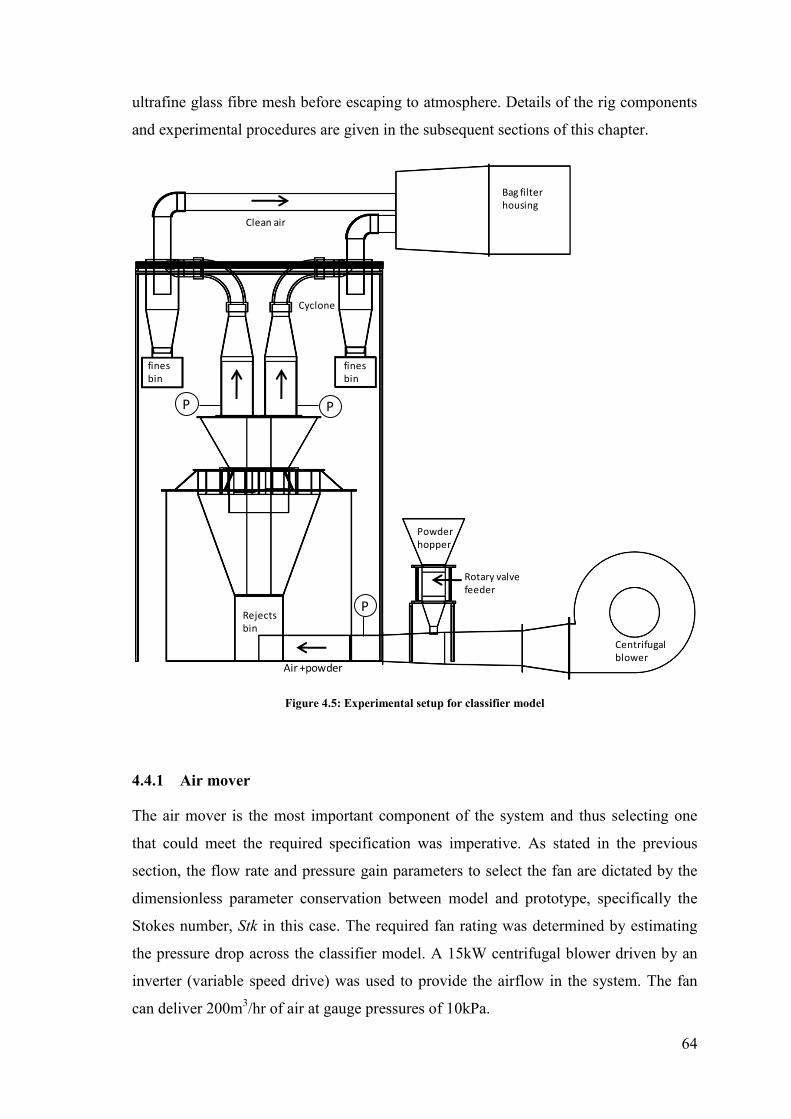
64

ultrafine glass fibre mesh before escaping to atmosphere. Details of the rig components

and experimental procedures are given in the subsequent sections of this chapter.

Figure 4.5: Experimental setup for classifier model

4.4.1 Air mover

The air mover is the most important component of the system and thus selecting one

that could meet the required specification was imperative. As stated in the previous

section, the flow rate and pressure gain parameters to select the fan are dictated by the

dimensionless parameter conservation between model and prototype, specifically the

Stokes number, Stk in this case. The required fan rating was determined by estimating

the pressure drop across the classifier model. A 15kW centrifugal blower driven by an

inverter (variable speed drive) was used to provide the airflow in the system. The fan

can deliver 200m3/hr of air at gauge pressures of 10kPa.

Powder hopper

Rotary valve feeder

Centrifugal blower

Bag filter housing

Air +powder

fines bin

fines bin

Cyclone

Clean air

P

PP

Rejects bin

65

Figure 4.6: Images of the experimental facility (LHS) and a view of the outlet section (top right) and inside the

classifier (bottom right).

The fan is connected to the classifier via a 1.2m duct which tapers out in order to match

the classifier tangential inlet duct width. Vibration of the rig by the fan is eliminated by

using a plastic vibration damping material to connect the fan outlet to the adapter. The

inlet velocity is measured at the powder feed location with a standard Pitot-static tube.

A traverse is taken across the duct to obtain dynamic pressure readings which are then

processed to obtain air velocity and mass flow rate. (Fig 4.7) The inlet air velocity can

be varied using the inverter drive, which controls the fan motor frequency (50Hz),

hence the volumetric flow rate. The volumetric flow rate is determined by calculating

the area under the velocity - cross sectional area curve, obtained from the Pitot tube

traverse. The required fan motor frequency for each inlet velocity condition is obtained

by calibration (Fig 4.8), giving a linear trend, with Goodness of fit R2 = 1.

66

Figure 4.7: Inlet velocity profiles for various air mass flow rates

Figure 4.8: Motor frequency setting as a function of average inlet velocity.

The inflow air temperature was measured by a K-type thermocouple located inside the

inlet duct. The inflow absolute air pressure was determined by adding the laboratory

ambient pressure, measured using a mercury in glass column barometer, to the

centrifugal fan outlet gauge pressure, by averaging the static pressures measured at all

four inlet duct faces with four Pitot tubes. The inflow air density was computed by the

equation of state for ideal gases with the specific gas constant R = 287J/kg K. Finally,

the inflow air flow rate was estimated by the product of the air density times the inflow

volumetric flow rate as determined by the integration of the inflow velocity profiles

from the Pitot anemometer.

4.4.2 Conveyed Material

As stated in section 4.4, a material other than coal has been chosen to simulate the

pulverised fuel in a working industrial classifier. This material commercially known as

0

2

4

6

8

10

12

14

16

18

20

22

0 0.1 0.2 0.3 0.4 0.5

Inle

t velo

ciy

(m

/s)

Cross sectional position (m)

Inlet mass flow rate =1.4kg/s

Inlet mass flow rate = 1.7kg/s

Inlet mass flow rate = 0.7kg/s

y = 0.6866x + 0.591R² = 1

6

8

10

12

14

16

18

20

5 10 15 20 25 30

Avera

ge inle

t velo

city (

m/s

)

Motor frequency (Hz)

67

Fillite, is an inert, hard, free flowing material made from alumina silicate spheres. The

density of the material is lower than that of coal, which is typically1300kgm-3

for

anthracite, such that conservation of the dimensionless Stokes number, Stk can be

achieved. The particle density is approximately 800kgm-3

and is a derivative of

pulverised fly ash. The particle size distribution is representative of the distribution

produced by comminution and fits the Rossin Rammler function (Scott, 1995). The

fillite size distribution was measured using particle counting in scanning electron

microscopy (SEM) images and standard dry sieving methods. A sample of the scanning

electron microscope image is given in figure 4.9. The two methods are in good

agreement as shown in Figure 4.10.

Figure 4.9: Microscopic image of the unprocessed feed fillite.

Figure 4.10: Cumulative size distribution (CSD) of feed fillite. A comparison of measured size distributions

using image size analysis and standard dry sieving methods.

0

10

20

30

40

50

60

70

80

90

100

0 20 40 60 80 100 120

Cu

mu

lati

ve u

nd

ers

ize

(%

)

Particle size x (µm)

Image analysis

Sieve

68

Physical Properties of Fillite

Average particle density (kg/m3) 800-900

Average bulk density (kg/m3) 400-480

Packing factor 60-65%

Hardness (Mohrs scale) 6

Average wall thickness (% sphere diameter) 5%-10%

Melting temperature (°) 1400

Thermal conductivity (Wm-1

K-1

) 0.11

Loss on ignition 2% maximum

Surface moisture 0.3 maximum

Crush strength (kg/cm2) 140-280

Table 4.3: Physical properties of conveyed material from (www.fillite.com)

Chemical Properties

Shell

34%-39%

55%-65%

2%

Gas Carbon Dioxide 70%

Nitrogen 30%

Table 4.4: Chemical properties of conveyed material.

Physical and chemical properties of the Fillite are displayed in tables 4.2 and 4.3.

4.4.3 Particle feeding device

The particle feeding device used in this study is the rotary valve feeder, which is

commonplace in pneumatic conveying installations. A sketch of the rotary valve feeder

is given in Figure 4.11. Due to the positive pressure system configuration of the

classifier, the material has to be fed against a positive pressure gradient and as a

consequence, this presents an air leakage problem. However, the pressure loss was

minimal and the air did not affect the gravity flow of material into the feeder. As a

precaution, the storage hopper was closed after loading, to prevent any material

backflow. The most significant aspect of selecting the feeder was its capacity to break

up the particles during the rotary feed. This would be undesirable as control of the feed

size and shape of the feed particles would be lost. A test run showed that the outlet

product was not significantly affected by the feeder and that particles generally kept

their size and shape, as shown in Figure 4.12. The rotary valve used was a DRV Britton

Protocol valve with 8 close end blades with ‘deep pockets’, and a direct drive motor.

69

The motor was connected to an inverter drive to enable variation of the rotor speed to

control the powder volumetric flow rate and the solid loading.

Figure 4.11: Generic drop-through rotary valve (Mills, 2004).

Figure 4.12: Scanning electron microscope image of a powder sample collected from the cyclone hopper.

Particles are generally intact.

At the rotor top speed of 22rpm (0.37Hz), the feeder delivers a volumetric flow rate of

0.85ltr/s which corresponds to a powder mass flow rate rate of 0.763kg/s. In order to set

the desired powder (fillite) flow rate, the feeder was calibrated by plotting fillite mass

flow rate against the corresponding rotor speed in rpm.

70

Figure 4.13: Rotary valve calibration chart

4.4.4 Flow measurement and instrumentation

As explained in section 4.4.1, the mass flow rate of air was controlled by a variable

speed drive calibrated against a Pitot-static tube traverse of the inlet cross section.

1.5mm diameter steel pressure taps were positioned on the four faces of the inlet duct

and connected via tubing in order to measure the average inlet static pressure and the

pressure drop across the classifier model. The tappings were installed in line with the

BS 848 specification. The pressure is measured using an electronic manometer

connected to a Labview program that was developed to acquire large samples of

pressure data at high sample rates. A study was performed to determine the number of

samples required (2000) to obtain convergence with standard deviations from the mean

generally less than 0.01%.

Cross sectional velocity measurements inside the body of the classifier were performed

using an in-house 5-hole pressure probe or yawmeter, capable of resolving the three

velocity components. The 5-hole probe is further detailed in section 4.4.4.1. Orifice

plates designed to the BS 1042 standard were utilised to measure the flow rate at each

outlet. The mass flow split of air at the outlets is an important performance parameter of

classifiers as equal air-fuel distribution to each burner line is key for an efficient

combustion.

y = 0.0016x2

R² = 1

0.000

0.200

0.400

0.600

0.800

0.3 5.3 10.3 15.3 20.3 25.3

Fill

ite m

ass flo

w r

ate

(kg/s

)

Rotor speed (RPM)

71

4.4.4.1 5- hole pressure probe description

A set of open ended tubes, grouped together to form a single unit, was used to

determine the flow angles (pitch, α and yaw, φ) and the three-dimensional velocity

components (axial, radial, and tangential velocities) derived from the total and static

pressures of the swirling gas. A schematic of the probe is presented in Figure 4.14.

There is a number of different yawmeters available for measuring flow magnitude and

direction (Bryer and Pankhurst, 1971). The most common probes are the two, the three

and the five hole probe. Due to the three-dimensional nature of the classifier, it was

necessary to use a 5-hole pressure probe with the holes arranged diametrically across

the pitch and yaw planes and one central hole. Because of the relative simplicity of

manufacturing a 5 hole probe, compared with the cost of purchasing one, it was decided

to design and build the yawmeter specifically for the 1/3 scale classifier model. It was

an added advantage to custom make one as the probe could be made to the length

required to traverse the 1.9 metre height of the rig. The probe consists of six

hypodermic 1mm steel tubes with four of the tube tips chamfered at 45 degrees secured

within a brass hemispherical head, adapted from the NPL pressure probe by Bryer and

Pankhurst, (1971). The six hypodermic tubes (including the static tube) are enclosed in

one single larger diameter copper stiffening tube for strength and robustness. A

thorough calibration over a matrix of pitch and yaw angles was performed. This

calibration is used to calculate the flow angles and velocities from the pressure readings

taken in the classifier model. A detailed description of the probe and of its calibration

methodology is presented in the subsequent section.

4.4.4.1 Probe calibration

The probe was calibrated at the University of Leicester, Defence Research Agency

(DRA) built low speed wind tunnel, capable of speeds of up to 40 m/s. The wind tunnel

is designed to produce a near one-dimensional, uniform flow at a low freestream

turbulence intensity. The probe was mounted with the head coincident to the tunnel

centreline and rotation in the pitch and yaw planes were performed manually, as

discussed in the next section.

72

Figure 4.14: 5-hole pressure probe used in the aerodynamic characterisation of the classifier scale model.

Figure 4.14(b): System of axes for describing motions imposed on pressure probes

Static pressure ports are installed two diameters downstream of the probe head and

azimuthal averaging of the static pressure readings is performed to obtain the average

static pressure. Figure 4.14(b) illustrates the system of axes that define the yaw and

pitch rotations.

y

x

y

Z

Static hole

ΨYaw

αPitch

windz

x

y

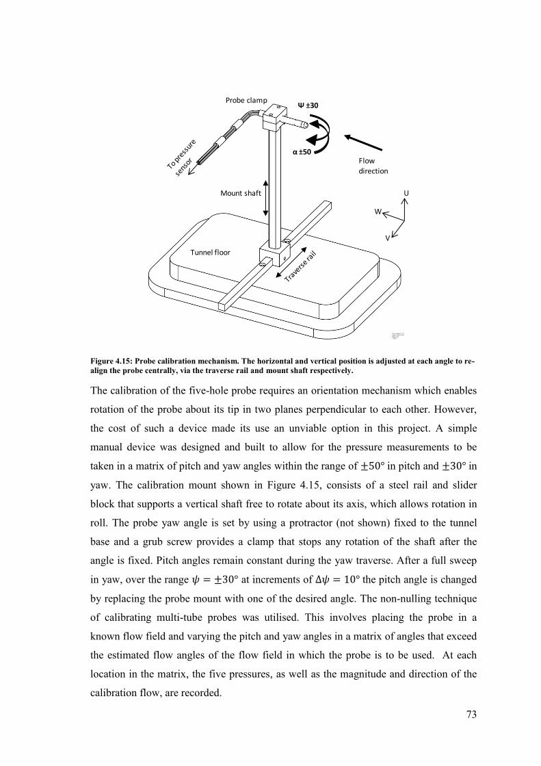
73

Figure 4.15: Probe calibration mechanism. The horizontal and vertical position is adjusted at each angle to re-

align the probe centrally, via the traverse rail and mount shaft respectively.

The calibration of the five-hole probe requires an orientation mechanism which enables

rotation of the probe about its tip in two planes perpendicular to each other. However,

the cost of such a device made its use an unviable option in this project. A simple

manual device was designed and built to allow for the pressure measurements to be

taken in a matrix of pitch and yaw angles within the range of in pitch and in

yaw. The calibration mount shown in Figure 4.15, consists of a steel rail and slider

block that supports a vertical shaft free to rotate about its axis, which allows rotation in

roll. The probe yaw angle is set by using a protractor (not shown) fixed to the tunnel

base and a grub screw provides a clamp that stops any rotation of the shaft after the

angle is fixed. Pitch angles remain constant during the yaw traverse. After a full sweep

in yaw, over the range at increments of the pitch angle is changed

by replacing the probe mount with one of the desired angle. The non-nulling technique

of calibrating multi-tube probes was utilised. This involves placing the probe in a

known flow field and varying the pitch and yaw angles in a matrix of angles that exceed

the estimated flow angles of the flow field in which the probe is to be used. At each

location in the matrix, the five pressures, as well as the magnitude and direction of the

calibration flow, are recorded.

α ±50

Ψ ±30Probe clamp

Mount shaft

Tunnel floor

Flow direction

U

V

W

74

To summarise the procedure, the probe was mounted on the holder at the tunnel

centreline at the desired pitch angle. The wind tunnel was set to the appropriate speed

and the pressures between the side holes were read in order to establish the zero yaw

position. This was the position in which the two side holes 2 and 4 in figure 4.14 read

the same total pressure. From this reference point, the probe was rotated to the next yaw

position up to in increments and locked in place by means of a grub screw

located at the base of the shaft. The six pressures were measured in turn (using a

scanivalve) and recorded with a LabView data acquisition program, taking 10,000

samples in a three second measuring window.

4.4.4.2 Calibration results and data reduction

The calibration data was converted into non dimensional pressure coefficients following

the procedure by Bryer and Pankhurst, (1971). These pressure coefficients are given in

equations 4.10- 4.12. The coefficients can then be used to estimate the pitch and yaw

angles as well as the total and the static pressures of the flow field from the calibration

data.

4.10

4.11

4.12

Where is the stagnation (total) pressure of the tunnel at a given speed, is the static

pressure and

. and were measured with an ellipsoidal

type L Pitot-static tube positioned at the tunnel centreline.

Bryer and Pankhurst, (1971) and Treaster, (1978) have shown that the relationship

between can be established by direct calibration at one

Reynolds number and can be applied to higher or lower Reynolds numbers, implying

the probe characteristics are independent of the operating conditions within limits. The

calibration was performed at two Reynolds numbers based on the

probe head diameter, in order to confirm its Reynolds number independence. The

difference between calibration constants at corresponding wind tunnel freestream

velocities of 7.5 m/s and 15 m/s were on average within 2%.

75

4.4.4.3 Resolving flow angles and velocity

There are a few different techniques in which the calibration data can be processed in

order to convert the measured pressures into the desired quantities such as flow angle

and mean velocity. Graphical methods and look-up tables have been used in the past by

Treaster, (1978) and Ligrani, (1989) where values around the constants are searched and

interpolations or local curve fits using these values are performed to obtain the results.

Some of the methods require a symmetric probe, so that a simplified set of overall curve

fits of the entire calibration data can be obtained. The manufacturing of an ideally

symmetric probe is costly and the use of look up tables obtained from the calibration

data can lead to increased uncertainties since a single bad datum point in the calibration

will affect the calibration constants and produce erroneous results. The analysis

technique used for the probe was one similar to that of Morrison et al, (1998). Here,

three-dimensional curve-fits of the entire set of calibration data were performed. The

method can be used with probes that may not be perfectly symmetrical about any one

plane and also contain erroneous points in the data set. However, it is important to select

the right type of functions to fit the data in order to avoid unrepresentative trends that

may incorrectly deviate from the raw data points even with a high goodness of fit. The

goodness of fit ( values, of the four calibration parameters were

0.993, 0.992 and 0.991 respectively. Rational functions were used to fit the and

data, which are defined as

4.13

where a, b, c , d, e, f and g are constants determined by the regression,

4.14

where h, i, j, k, l, m, n, o, p and q are constants determined by the regression,

4.15

A-J and K-S are also constants determined by the curve fit. The standard error of all fits,

which is an estimation of the standard deviation of the least square fits, was less than

2%. The three dimensional contour plots of each parameter are displayed in Figure 4.16

- Figure 4.18. Figure 4.16 and 4.17 shows the dependence of the yaw angle upon the

76

and coefficients. These surfaces relate to equations 4.13 and 4.14, and are a

visual representation of the curve fit. These plots along with Figure 4.18 can be used to

ascertain any probe imperfections in terms of symmetry or errors in the calibration

measurements. Figure 4.18 which shows the dependence of on the pitch and yaw angles

is characterised by concentric circles of constant as found also by Morrison, et al

(1998).

In the classifier, the probe was used to collect a set of six pressure measurements from

each tube (includes static tube) at discrete points in the model cross-section. The data

was reduced into the parameters of equations 4.10 - 4.12. Using these values the flow

angles and and the total pressure coefficient were estimated from equations

4.13 - 4.15. From these, the total pressure and mean velocity can be calculated from

4.16

4.17

where is the total (stagnation) pressure and is the static pressure. Furthermore, the

relationships between the velocity magnitude V and its components, in the probe

coordinate system are

4.18

4.19

4.20

where , and are the velocity components with respect to the cylindrical

coordinates as shown in Figure 3.1.

4.4.4.4 Error and uncertainty in calibration

The calibration and probe accuracy was determined by comparing velocity data derived

from the calibration constants and pressure measurements in the tunnel with known

velocities and probe angles. The calculated error in all the measurements was on

average 4.36%.

77

Figure 4.16: Calibration data showing the dependence of upon

Figure 4.17: Calibration data showing the dependence of upon

Figure 4.18: Calibration data showing the dependence of upon .

Ψ(°

)

Ψ(°

)

Cpα

CpΨ

α(°

)

α(°

)Cpα

CpΨ

Cp

5

Cp

5

Ψ(°

)

α(°)

78

4.4.5 Cyclone separator

Reverse flow cyclone separators are used in the experiments to recover the fine powder

leaving the classifier model. Its high separation efficiency, relative ease of manufacture,

and low cost make the cyclone an ideal separation device for the experimental rig

(Figure 4.5). The separator’s key function in the two-phase experiments is to recover all

of the particles allowed to exit the classifier so that they can be weighed and analysed,

in order to determine the outlet mass split and grade efficiency of the classifier. As a

result, the cyclone must be designed to produce a very small cut size and emit little or

no powder. In addition, the cyclone separator must be designed so as not to cause a high

pressure drop to the system.

The principle of the reverse flow cyclone operation is not too dissimilar to that of a

classifier. The particle laden flow enters the device tangentially, inducing a swirling

flow, the centrifugal force of which swings particles out towards the walls. The flow is

downward moving in the outer radial region and later reverses neat the cyclone axis,

where the clean gas exits the cyclone through the vortex finder tube.

Figure 4.19: Separation mechanism of a cyclone separator (Mills, 2004).

4.4.5.1 Cyclone design

The cyclone had to be designed around the existing rig and pipework. It was also

important to keep the diameter small in order to maximise the separation efficiency at

the operating conditions of the classifier model. A whole host of cyclone designs is

79

available in the literature, such as the Muschelknauts E & D, Storch 1-4 designs,

Tengbegen A-C, Van Tongeren and the Stairmand H.E design (Hoffman, 2008). All

cyclones can be categorised into either high throughput cyclones or high efficiency

cyclones (Figure 4.20). In the present work, the most important constraint, aside from

the high separation efficiency, was to design a compact unit that can be assembled

within the space constraints of the laboratory. The Tengbergen B cyclone shown in

Figure 4.21 was selected due to it fitting the size specifications required.

Figure 4.20: Performance curves for typical cyclone separators.

Figure 4.21: Schematic of a Tengbergen B cyclone showing the dimensional notation used herein (see table 4.5)

Dimensions and operating conditions are presented in Table 4.5.

a

Dx

D

S

H

Hc

Dd

80

Dimensional parameters

Inlet area A ( (mm2) 86.39

Vortex finder diameter Dx

(mm)

110

Vortex finder height S (mm) 223

Cyclone height H (mm) 604

Barrel length H-Hc (mm) 324

Underflow diameter Dd (mm) 112

Cyclone diameter D (mm) 212

Table 4.5: Dimensional parameters of the Tengbergen cyclone shown in Figure 4.21.

The dimensions in table 4.5 are based on the relative dimensional proportions of the

Tengbergen B cyclone as given by Abrahamsen and Allen, (1986). The cyclone used in

the experimental rig was designed to a scale which could fit the space requirements,

thus the separation efficiency and pressure drop needed to be determined for this

particular geometry.

4.4.5.2 Pressure drop predictions

The pressure drop of the cyclone was required in order to select the fan rating and

ensure any consequential drop would not affect separation performance. Cyclone

pressure drop models are abundant in the literature, some analytical (Barth, (1956),

Stairmand, (1949) and Muschelknautz, 1972) and others are empirical Shepherd &

Lapple, (1949) and Casal & Matinez, (1983) for example. The empirical models are the

more simplistic as they only account for losses in the inlet and outlet areas while the

models of Barth and Stairmand account for losses in the body and vortex finder and also

include the effect of solid loading (Hoffman, 2008). As only an approximate estimate of

the cyclone pressure loss was required for design purposes, it was decided to evaluate

the pressure drop models of Stairmand, (1949) and Casal, & Matinez, (1983) and to

design the system around the greatest predicted by the two models.

Firstly we present the Stairmand model as modified by Iozia and Leith, (1989)

4.21

Where is the inlet Euler number and is the inlet area

81

with

4.22

Where AR is the total wall area of the cyclone body including the inner walls of the

roof, the cylindrical and conical sections and the outer wall of the vortex finder. G is a

wall friction factor , which Stairmand set to 0.005 for cyclones operating at

low loadings while is the friction factor. (Hoffman, 2008).

=

4.23

The Casal and Martinez, (1983) empirical model predicts the normalised pressure loss

coefficients as

4.24

For the geometry and flow parameters in table 4.5, equations 4.21 and 4.24 give

predicted pressure drop values of 2492Pa and 3248Pa. The centrifugal fan was then

sized to compensate for the larger of these pressure drops.

4.4.5.3 Separation efficiency predictions

As mentioned in the section 4.45, a low cyclone cut size (x50) and high particle

collection efficiency is crucial to the success of the experiments. This is so because the

cyclone is required to recover most of the particles that leave the classifier. In this

section the cut size and grade efficiency of the cyclones are calculated in order to

estimate the particle size range and volume that may not be recovered by the cyclone.

Cyclone literature contains a number of models that can predict the separation

efficiency of a conventional cylinder-on-cone cyclone or swirl tube with good accuracy.

The basis of these models can generally be categorized into one of two concepts; the

‘equilibrium-orbit’ or ‘time-of-flight’ approach. The former is constructed from a force

balance (outward centrifugal and inward fluid drag force) on a particle rotating in the

imaginary cylindrical surface CS (imaginary surface extending below the vortex finder).

82

On the other hand, the time of flight model considers particle migration to the wall and

neglects the inward gas velocity. An example of the equilibrium orbit model is that of

Barth, (1956) and a modification by Muschelknautz, (1972). The original time-of-flight

model was proposed by Rosin et al, (1932), who compared the time required for a

particle injected through the inlet at some radial position to reach the cyclone body, to

the time available for this (Hoffman, 2008). However, these models are somewhat

outdated and limited in application with respect to cyclone design. The Muschelknautz

model on the other hand is a more recent and comprehensive model based on the Barth

equilibrium orbit model and is valid for all cyclones and swirl tubes. It has the ability to

account for the effects of wall roughness due to both the construction material and the

presence of solids. In addition, the model can account for a change in the particle size

distribution of the feed particles into the cyclone. As a result, the model is capable of

predicting the separation efficiency of cyclones to a high level of certainty. (Hoffman,

2008) The Muschelknautz, (1972) method of modelling cyclone separation is thus

utilised in the prediction of the cyclone performance parameters. The equations required

to evaluate the cut size and hence derive the grade efficiency of the cyclone are

presented below.

The entrance constriction coefficient for a ‘slot-type’ inlet is given by Muschelknauts

and Trez, (1997) empirically as

4.25

Where

=b/R (where b is the cyclone inlet duct width), co is the solid loading

ratio, and R is the cyclone outer radius as shown in Fig 4.22. The tangential velocity

at the control surface (CS) of the vortex finder determines the cut size of the

cyclone however, the near wall velocity, (Fig 4.22) is required to evaluate this. This

is found using the equation below

4.26

Figure 4.22 introduces illustrates that is the distance from the cyclone centreline to

the centre of the inlet duct notation used in the calculations including Rin as presented

83

above. The wall axial velocity, (Fig 4.22) is also required in evaluating the friction

factor is estimated as.

4.27

where Q is the air volumetric flow rate and Rm is the geometric mean radius given by;

Figure 4.22: Plan view of a typical cylinder- on-cone cyclone showing additional parameters required to

calculate cyclone cut size (Hoffman, 2008).

4.28

As shown in Figure 4.22, 10% of the incoming flow is estimated to short-circuit the

main body and flow radially inwards and exits the cyclone. The factor of 0.9 in Eqn.

4.27 represents the resulting flow participating in the main flow along the walls and

contributing to the inner vortex. This inner vortex has a major influence on the cut size

of the cyclone.

The final parameters required to compute the cut size is the gas only friction factor

and the combined gas solid friction factor . Muschelknautz and Treyz, (1991)

showed that is a function of the cyclone body Reynolds number

4.29

A chart of the aforementioned along with a mathematical function to fit the curves was

presented by the authors. This can be seen in chapter 6 of (Hoffman, 2008). They also

84

noted that there is an added friction contribution to the air friction factor; this is from

the relative wall roughness, ( Ks/R . The empirical curve fit is given below;

4.30

4.31

4.32

The total frictional factor can be computed using the relation given by Muscheknautz

as (Hoffman, 2008)

4.33

Finally, the tangential velocity of the gas at the ‘inner core’ radius RCS (see Figure 4.22)

can be calculated using the following expression (Hoffman, 2008)

4.34

The cut-point diameter is (Hoffman, 2008)

4.35

The grade-efficiency of the cyclone can be computed using various methods but a

simple and practical solution is given by

4.36

The exponent m can be set between 3 and 5. The value of 5 is chosen based on validated

predictions from similar designs and operating conditions as reported by Hoffman,

(2008).

85

Figure 4.23: Predicted grade efficiency of the Tengbergen cyclone used in the classifier experiments.

The overall collection efficiency was evaluated by dividing the feed into seven size

fractions, each fraction comprising a known fraction of the total mass of feed solids.

These values were multiplied by the fractional efficiency derived from the grade

efficiency curve and a summation of all seven fractions results in a value for the overall

separation efficiency. This can be written mathematically, in discrete form as

4.37

Table 4.6: Model results for parameters used in the cut size and pressure drop calculations.

where is the ith

mass fraction. The values of the parameters required to calculate

the separation efficiency and pressure drop are listed in table 4.6. The estimated

separation efficiency of the classifier was 98.2% with a 50% of the collected particles

being less than 2.5 µm.

0

0.5

1

0 5 10 15 20 25

Frac

tio

nal

eff

icie

ncy

(η)

Particle size (µm)

0.9 26.3

16.5m/s 2.5µm

14.18m/s 98.2%

0.073 4.34x10-4

5.81x105 0.46

0.0153 3248

86

4.5 Particle size analysis

Particle measurement has been performed using an off-line method, where particles are

collected and subsequently analysed outside of the sampling environment. This is in

contrast to on-line methods with which particle size distribution measurements are made

in real time (Nguyen et al., 1989).

Two methods were used initially to analyse the particle size distributions of both the

reject and the outlet streams. The results of the methods were compared, and although

they did not disagree significantly, the image analysis method was retained and used for

all of the samples. The reason is because only a small sample was required for the

microscopic analysis, therefore sample preparation, which consisted mainly of

agglomerate dispersion, was easily conducted and in a timely fashion. Numerous

samples (5-7) were analysed to ensure the samples taken were representative of the

powder collected in the cyclone and classifier reject hopper. Also it is stated in the

literature that dry sieving should be limited to particle sizes less than 75 microns. A

brief description of the sizing methods is given in the subsequent sections.

4.5.1 Sieve Analysis

Sieve analysis determines the gradation or distribution of particle sizes within a given

sample. Apparatus utilised include a scale readable to 0.01g that meets the requirement

of AASHTO M-231, (1995) a number of standard sieves (106µm-45µm) that meets the

requirement of AASHTO M-92, (2010) and a mechanical sieve shaker, which meets the

requirements of AASHTO T-27, (2006). The sieves were nested in order of decreasing

size before the samples were poured in and the shaker ran for approximately 15 minutes

per sample. The result of the sieve analysis is a mass or weight distribution by size, and

can be used to derive a cumulative particle undersize distribution, which is more useful

in describing the performance of a classifier or pneumatic separator as the cut size is

obtained from this cumulative distribution.

The mass distribution can be fit to a standard model function called the Rosin Rammler

distribution (Allen 1990).

4.5.2 Image analysis

The spherical nature of the Fillite particles allowed a fairly straightforward

measurement of the diameter, providing the particles were stable in orientation on the

87

slide. Counting of the measured particles was done by acquiring multiple images of the

same sample from a scanning electron microscope (SEM) which were then analysed on

dedicated software called ‘analySIS docu’ developed by Olympus Soft Imaging

Solutions. The SEM can resolve particle sizes from 1mm down to 20nm.

4.5.3 Particle measurement

The sizing method used in the analysis is somewhat novel. It is based on an adaptation

of a standard optical microscopy technique which uses a British standard graticule as

described in Allen, (1997). The method is in line with the British standard (BS3406-4,

1993).

With image analysis, individual particles of varying size are counted but this then has to

be converted from a number count to a mass count as a size distribution by weight is

required. The percentage by weight in each class is:

4.38

Where is the number of particles in j classes of mean size xr found in the sample

area Direct conversion from a number count to a mass count is not straight-

forward, because the omission of a single particle in the largest size class can be

equivalent to the omission of tens of thousands particles in the smallest class. Hence

statistical controls were imposed to ensure precision and repeatability in the

measurements. For a particle size analysis by mass, in order to obtain an estimated

standard error of less than 2%, 25 particles in the largest size category have to be

counted (Allen, 1997). The expected standard error of the percentage in each

size class, out of the total weight in all size classes, was calculated as (Allen, 1997)

4.39

The number of particles counted in the respective size classes is governed by the

number count in the control size and the required accuracy, given by

4.40

where is the standard deviation expressed as a percentage by weight in the size

class, out of the total weight, is the percentage by weight in the given size range and

88

is the number of particles counted in that size range. The number density is

calculated in order to determine the number of similar areas to scan for particles in that

particular size range.

4.41

where A is the required scan area for a size class. The suffix ‘0’ denotes the control

class, which is the class containing the most particles by weight, which is usually the

top (largest) size class. Thus, A0 is the control class scanned area, N0 is the control class

number density and X0 is the median size of the control class particle size range. Due to

the requirement of having a minimum of 25 particles in the largest size category, the

area to be examined must decrease with decreasing particle size to avoid the required

counts running up to millions. The requirement of detecting 25 particles in the top size

range is a first approximation and this number may increase or decrease depending on

the percentage of the total weight occupied by this size range. This is controlled by Eqn.

4.39.

To summarise the analysis procedure,

A small sample is taken from one of the product streams for each experimental

case. Initially, the particles were prepared by agitating in a water suspension to

remove agglomerates. It was later found that the fillite material recovered was

readily dispersed, however, this was ensured by brushing the particles off unto a

slide (8mm diameter) covered by a sticky material.

The slide is mounted in the SEM chamber which is run in the wet mode. This

gives a better image than a standard setting. Five isolated areas or ‘fields’ across

the slide are scanned at four incremental magnifications shown in table 4.7.

Images are acquired and transferred to the analysis program. The particle Feret

diameter (Walton, 1948) (Figure 4.24) is measured for individual particles.

89

Figure 4.24: From top to bottom, and left to right; SEM images of a typical coarse sample from the classifier at

80x 120x, 200x and 350x magnification. Particle counts in each image are based on the requirement of a

resulting standard error of less than 2%

During size analysis, a set of size classes is chosen and particle counts are

allocated to each class. The class sizes selected in the present investigation are

reported in Table 4.7. The top size class is the control class where at least 25

particles are counted. First, a preliminary scan is performed to determine the

particle number density in a given image area for each size

class using the same image magnification. The area required (or number of

images) to count 25 particles in the control size class is then calculated.

Next, the number of scans, or the required scan area for the remaining classes is

calculated using Eq. 4.41. The required area is scanned for particles in each size

class until there is no uncounted particle in the region.

The process is then repeated at a higher magnification.

A minimum of 700 particles are counted in each experimental case, with

standard errors (as given in Eq. 4.40) kept to a maximum of 2%.

90

Class Size Limits (µm) Required Magnification

1 108-75 80x 2 75-65

3 65-54 120x 4 53-43

5 43-32 200x 6 31-21

7 20-2 350x

Table 4.7: Particle size classes and their limits, Magnification is increased in order to size accurately the

smaller particles.

4.6 Conclusions

A description of the experimental rig used in the classifier study has been presented in

this chapter. Dimensional analysis has been used to ensure the results generated from

the model are applicable in full scale. However, the rig was shown to be unable to

obtain an air-fuel ratio matching that of power stations and the Reynolds number is an

order less than that of the prototype. It is assumed that the lack of total conservation of

these parameters still allows the application of some of the findings from this study to

the classifier prototype. Overcamp and Scarlett, (1993) presented extensive data in their

study that supports this assumptions by showing that the Stokes number is constant over

a wide range of Reynolds numbers above 2 x 104. The rig instrumentation and particle

analysis methods were detailed along with the design and calibration of a 5 hole Pitot

tube capable of measuring the three-velocity components and the static and stagnation

pressures inside the classifier model.

92

Chapter 5

Classifier Air Flow Characterisation

5.1 Introduction

Optimising the separation efficiency and other performance parameters of classifiers

involves understanding how the particles behave in the separation space. To do this the

velocity distribution of the air phase and the variables that control it must be

determined.

In this chapter, a thorough experimental investigation is conducted to determine:

The effect of inlet flow uniformity on the velocity profile outside and inside the

main separation region as well as the outlet air mass flow rate or distribution

between the multiple outlet pipes.

The distribution of the tangential, axial and radial velocity components. Powder

experiments will be conducted to relate the velocity distribution with the

classifier performance parameters to identify optimum or favourable flow

distributions.

The effect of the vane angle on all velocity components will be established by a

set of measurements at cone vane angles ranging from 30 to 60 degrees from the

tangent of the pitch diameter as illustrated in Fig. 3.6 of chapter 3.

If there is a correlation between swirl intensity and inter-outlet air flow rate

distribution.

Whether there are similarities between the flow pattern of a cyclone separator

and that of a classifier. A simple model that describes velocity distribution in

cyclones will be fitted to the model results.

93

5.2 Swirl number

Swirl intensity can be quantified by the swirl number S, which is defined as the ratio of

tangential momentum flux to axial momentum flux given as (Gupta et al., 1984)

5.1

where the tangential momentum flux and is the axial momentum flux. The swirl

number analysis is reported for the three geometries described in chapter 4. One of

which is the benchmark classifier model shown in Figure 4.1 and the static port ring

(SPR) models of Figure 4.2(a) and 4.2(b), which have inlet blade angles of 30 and 45

degrees respectively. In each of these designs, measurements of the axial and tangential

velocities at two inlet velocities (7.3 m/s and 14.3 m/s) were taken, and the swirl

numbers were calculated using equation 5.1. The results showed that the inlet swirl is

independent of the inlet velocity as the swirl numbers calculated for the aforementioned

velocities were within 2% for all three geometries.

The radial distribution (normalised by the classifier radius Rclass) of the tangential

momentum flux and the axial momentum flux for the three inlet configurations are

plotted in Figure 5.1-Figure 5.3. Tangential and axial momentum flux data for the TIC

inlet configuration, SPR30 and SPR45 configurations are displayed in figure 5.1, figure

5.2 and figure 5.3 respectively. The swirl number in the benchmark model has been

predetermined by attainment of geometric similarity with a prototype spindle mill

classifier under a high Reynolds number (inviscid flow) assumption.

The static port ring designs of figure 4.2 give the reported lower swirl numbers in table

5.2 due to the flow deflecting blades that form the nozzle boundary. The axial velocity

component is increased as a result of the steep blade positioning hence, the swirl

number decreases as dictated in equation 5.1. The greater axial velocity component

ensures particle entrainment and carriage to the main separation zone, which is inside

the concentric cone; however, too large a reduction in swirl would compromise the first

stage centrifugal separation that occurs in the annulus.

94

Figure 5.1: Cross sectional profiles of the tangential and axial momentum fluxes at near inlet location for the

TIC inlet configuration at normalised axial location y/Dc=0.45.

Figure 5.2: Cross sectional profiles of the tangential and axial momentum fluxes at near inlet location for the

SPR30 inlet configuration at normalised axial location y/Dc=0.45.

Figure 5.3: Cross sectional profiles of the tangential and axial momentum plots at near inlet location for the

SPR45 inlet configuration at normalised axial location y/Dc=0.45.

0

0.001

0.002

0.003

0.004

0.005

0.006

0.007

0.008

0.3 0.5

Gθ

(Ns-1

m-2

)

r/Rclass

TIC-Tangential flux- 0.115

0

0.001

0.002

0.003

0.004

0.005

0.006

0.007

0.008

0.3 0.5

Gz

(Ns-1

m-2

)

r/Rclass

TIC-Axial flux -0.106

0

0.005

0.01

0.015

0.02

0.025

0.3 0.5

Gθ

(Ns-1

m-2

)

r/Rclass

SPR30-Tangential flux - 0.42

0

0.005

0.01

0.015

0.02

0.025

0.3 0.5

Gz

(Ns-1

m-2

)

r/Rclass

SPR30 - Axial flux - 0.6

0

0.005

0.01

0.015

0.02

0.025

0.03

0.035

0.04

0.3 0.5

Gθ

(Ns-1

m-2

)

r/Rclass

SPR45- Tangential flux - 0.53

0

0.005

0.01

0.015

0.02

0.025

0.03

0.035

0.04

0.045

0.05

0.3 0.5

Gz

(Ns-1

m-2

)

r/Rclass

SPR45- Axial flux - 1.07

95

5.3 Airflow distribution

It was found in the preliminary experiments on the benchmark model that due to the

entry conditions, the velocity distribution across the classifier was not axisymmetric.

The full radial profile across the classifier at several axial positions is given in appendix

B. Plant measurements and simulations by (Shah et al., 2009) also show gross air flow

asymmetry. It is important to determine whether this extends beyond the annulus and

manifests itself at the outlet pipes either causing or exacerbating the problem of the

uneven distribution of solids commonly encountered in the burner feeding lines.

Without active control of the outlet flow using gates and valves, the distributions of

both air and coal at the outlets frequently exceed the allowed deviation margin of ±10%

for air and ±15% for coal in pulverised fuel power plants. The experiments aim to

determine the factors contributing to the imbalance.

As a potential flow modifier, a nozzle or port ring was developed as described in section

4.2.1 in order to promote flow axisymmetry in the classifier model. The port ring blade

angles are adjustable, so that the swirl intensity may also be varied. They have not been

aerodynamically designed as their function in the current work is only to provide a

means of evenly distributing the flow and thus providing an extra design variable.

However, CFD simulations were performed to ascertain the macro effects of the blades

on the flow in order to aid its design.

It should be noted that in their description the static port ring models are prefixed with

‘inlet’ to specify that its location is upstream of the main separation zone and is not as

an inlet medium to the pulveriser mill itself. The term ‘inlet model’ is used to

distinguish between the benchmark model and the two port ring variations.

Flow measurements were conducted using the 5-hole pressure probe introduced in

section 4.4.4. 10,000 samples of total pressure were acquired at each hole, from which

measurements of static pressure and of the local velocity vector, expressed by its three

Cartesian components were derived from Eqs. 4.16-4.26. The difference in flow

uniformity between the static port ring models of (SPR30 and SPR40) and the tangential

slot inlet (TIC) is discussed in section 5.3.1.

96

5.3.1 Circumferential velocity profiles

Ideally one desires a uniform velocity distribution around the classifier circumference to

avoid areas of high velocity that may entrain larger coal particles higher than the cut

size. Also a low local velocity may cause mass drop out of coal within the cut size,

which is undesirable and may cause fires at the bottom of the mill (Storm, 2009).

Figure 5.4: Location of the angular reference points. Measurement pitch diameter on the cylindrical surface in

which the measurements apply.

Figure 5.5-Figure 5.7 shows the mean velocity distribution in the classifier models with

and without the flow distributing port ring at the angular positions around the model

shown in Figure 5.4. All measurements are performed at a radial distance r0 = 45° from

the cylindrical axis. Only the results from the SPR30 model are presented here for

brevity, as the difference in distribution between these and the SPR45 model

measurements are minimal. The standard deviation of the normalised velocity

magnitude (Vm/Vin) around the circumference was estimated as a measure of how

uniform the flow velocity around the circumference is. A low value of the standard

deviation indicates a more circumferentially uniform flow. Firstly, by comparing the

standard deviations between TIC and SPR30 in Figure 5.5, it is clear that with the inlet

guide vanes installed, the flow is more axisymmetric. These results are consistent at

both normalised axial positions with the higher of these possessing the lowest standard

deviation.

0°

270°Inlet duct

90°

180°

Measurement pitch diameter

97

Design Vin (m/s)

Cone vane

angle (°)

Standard deviation (m/s)

y/Dc= 0.46 y/Dc =1.04

SPR30 14.3 30 0.82 0.51

SPR30 14.3 45 0.73 0.27

TIC 7.4 30 0.68 0.43

TIC 7.4 45 0.66 0.36

TIC 7.4 60 0.88 0.37

TIC 14.3 45 1.19 0.84

TIC 14.3 60 1.25 0.75 Table 5.1: Circumferential flow uniformity variation with inlet design and operating parameters. Measured as

the standard deviation of the average.

The circumferential distribution of air velocity magnitude also appears to be a function

of the cone vane angle. Table 5.1 shows that a decrease in the cone vane angle reduces

the radial flow area into the cone, which causes a reduction in the circumferential flow

uniformity. This is likely to be due to the associated rise in tangential velocity and an

increase in the local turbulence intensity.

Figure 5.6 compares the circumferential velocity profiles at two different inlet velocities

of Vin = 7.4 m/s and Vin = 14.3 m/s in the benchmark (TIC) model. The results at both

cone vane angles of 45°, figure 5.6 (a) and of 60° in figure 5.6 (b) show that a lower

inlet velocity of 7.4 m/s provides a circumferentially more uniform flow, which reduces

the normalised standard deviation of velocity magnitude by about 1/3 at a cone vane

angle of 60° and by almost ½ at a cone vane angle of 30°.

Finally and perhaps the most important observation is the improvement in uniformity of

the circumferential velocity profile as the flow progresses to the upper region of the

classifier. With time, the velocity equalises itself around the circumference in which the

uniformity (quantified by the standard deviation) is improved by at least 37% in all the

cases, and up to 65% when the static port ring is used at a cone vane angle of 60°. This

is illustrated by the reduction in the standard deviation, σ = 0.66 from the normalised

axial position of y/Dc=0.46 and inlet an velocity of 7.4 m/s as shown in figure 5.6 (a), to

a standard deviation of σ = 0.36 at y/Dc=1.04 in figure 5.7(a), for the same inlet

velocity. This trend of decreasing standard deviation with increasing axial position is

also observed for the 60° cone vane angle of figures 5.6(b) and figure 5.7(b).

98

a) (b)

Figure 5.5: Circumferential variation of the normalised mean velocity for different inlet designs. The standard

deviations about the average values in the profile are shown for both models. Measurements are taken at (a)

y=550mm and (b) y=1250mm. Inlet velocity Vin = 14.4m/s.

(a) (b)

Figure 5.6: Circumferential variation of the normalised mean velocity for 45 and 60 degree cone vane angles-

(a) and (b) respectively. Effect of inlet velocity is shown for measurements in the TIC inlet design at axial

position Y = 550mm (y/Dc =0.46)

(a) (b)

Figure 5.7: Circumferential variation of the normalised mean velocity for 45 and 60 degree cone vane angles-

(a) and (b) respectively. Effect of inlet velocity is shown for measurements in the TIC inlet design at axial

position Y = 1250mm (y/Dc =1.04)

0

0.5

1

1.5

2

0 60 120 180 240 300 360

Vm

/Vin

angle (°)

TIC Standard deviation = 1.19SPR30 Standard deviation = 0.73

0

0.5

1

1.5

2

0 60 120 180 240 300 360

Vm

/Vin

angle(°)

TIC Standard deviation = 0.84SPR30 Standard deviation = 0.27

0

0.2

0.4

0.6

0.8

1

0 60 120 180 240 300 360

Vm

/Vin

angle (°)

Vin-14.3m/s Standard deviation = 1.19Vin-7.4m/s Standard deviation = 0.66

0

0.2

0.4

0.6

0.8

1

0 60 120 180 240 300 360

Vm

/Vin

angle(°)


0

0.5

1

1.5

2

0 60 120 180 240 300 360

Vm

/Vin

angle(°)


0

0.5

1

1.5

2

0 60 120 180 240 300 360

Vm

/Vin

angle(°)

Vin-14.3m/s Standard deviation = 0.75Vin -7.4m/s Standard deviation = 0.37

99

An alternative solution to the distribution problem could be to extend the height of the

classifier, given that the flow tends to even out with time. Later in this chapter it will be

shown whether this translates to a better cross-sectional distribution of the velocity

magnitude in the cone and a more even balanced air mass flow distribution among the

outlet pipes.

5.3.2 Inter-outlet mass flow balance

The air flow rate at the outlet pipes was measured by orifice plates fitted to each of the

individual outlets. Although most of the swirling flow decays by the time it reaches the

outlets, there is still some spin present. This tends to reduce the accuracy of the orifice

flow measurements if the swirl not calibrated for. Therefore, the flow rates were

calibrated against mass flow rates obtained from velocity traverses across each pipe

diameter, results in an average error of 7.4 %. The four outlets of the classifier model

were numbered for identification as shown in figure 5.8

.

Figure 5.8: Schematic of the classifier outlet configuration with numbered outlet pipes.

Figures 5.10, 5.12 and 5.14 show the percentage deviations from the mean of the total

air mass flow rate out of the classifier model. The mass flow deviation mD, is plotted for

each of the outlets shown in figure 5.8 at various inlet mass flow rates and cone vane

angles (30°, 45° and 60°) for the benchmark model TIC and the static port ring models

SPR30 and SPR45. A comparison among the three inlet model variations shows some

surprising results. The port ring models SPR30 and SPR45, with their more uniform

annular flow, fail to provide a more even inter-outlet flow distribution than the baseline

TIC configuration at all three vane angles. Figure 5.12, Figure 5.14 and Figure 5.10

shows the normalised standard deviation of air mass flow rate computed among the four

4 1

3 2

100

outlets of Figure 5.8 for the TIC, SPR30 and SPR45 inlet configuration. The analysis on

the effect of vane angle shows that a more even distribution of airflow among the four

outlets is obtained by decreasing the cone vane angle. A computation fluid dynamic

investigation on the effect of the cone vanes on the classifier airflow (Afolabi and

Aroussi, 2010) showed that decreasing the vane angle, as shown in Fig. 3.6, increases

the swirl intensity in the cone and in the outlet region. Therefore an important

conclusion to draw from these results is that, the swirl intensity in the outlet region,

controlled by the cone the vane angle, is more important to obtaining an even airflow

distribution among multiple outlets than ‘inlet’ or annular flow uniformity in the model

classifier. This is illustrated more clearly in Table 5.2, which reports the air mass flow

rate percentage deviation averages over all of the operating inlet mass flow rates. Table

5.2 shows that increasing the cone vane angle increases the difference in the air flow

rate output among the four outlets.

Finally, it has also been shown that the inter-outlet air mass flow rate distribution is a

function of inlet air mass flow rate or velocity. The relationship is positively correlated,

with SPR45 displaying a linear trend for ζ =30° and ζ =45° as well as the TIC inlet

configuration, for ζ =60°.

Mean deviation (%)

Cone Vane Angle (°) TIC (S=1) SPR30 (S=0.7) SPR45 (S=0.49)

30 7.04 7.61 8.6

45 9.9 10.2 13.21

60 13.8 24.3 19.8

Table 5.2: Average percentage deviation in air mass flow rate across the four outlets at different vane angles

and inlet configuration. Swirl numbers corresponding to inlet configuration is shown in brackets.

5.4 Classifier flow pattern

In this section, results of cross-sectional measurements in both the annular and the

separation zones of the classifier are presented. Measurements are taken at three

different axial stations as detailed in Figure 5.15(b) and across two perpendicular

meridional planes at θ = ± 45° as shown in Fig. 5.16(a). However, for brevity, only the

results on the θ = + 45° meridional plane identified by the arrows in Fig. 5.15(a) are

presented below in the remaining sections of this thesis. Axial positions are normalised

by the classifier diameter Dc, whereas radial positions are normalised by the classifier

radius Rc.

101

(a) (b)

(c)

Figure 5.9: Mass flow deviation (%) from the mean of the air phase as a function of inlet mass flow rate. (a)

ζ=30°, (b) , ζ=45°and (c) ζ=60° cone vane angle settings in the TIC inlet design.

Figure 5.10: Standard deviation of the average air mass flow rate between the outlet pipes at different inlet

flow rates (0.79, 1.07, 1.4, and 1.729kg/m3) for the TIC inlet. Each curve represents a cone vane angle ( )

setting.

-15

-10

-5

0

5

10

15

0.729 1.07 1.41 1.739

Outlet 1

Outlet 2

Outlet 3

Outlet 4

𝒎𝑫(%)

𝑚𝑎 (kg/s)

-30

-20

-10

0

10

20

30

0.729 1.07 1.41 1.739

Outlet 1

Outlet 2

Outlet 3

Outlet 4

𝒎𝑫(%)

𝑚𝑎 (kg/s)

-30

-20

-10

0

10

20

30

0.729 1.07 1.41 1.739

Outlet 1

Outlet 2

Outlet 3

Outlet 4

𝒎𝑫(%)

𝑚𝑎 (kg/s)

0

0.005

0.01

0.015

0.02

0.025

0.03

0.035

0.04

0.045

0.05

0.5 0.7 0.9 1.1 1.3 1.5 1.7 1.9

ζ = 30

ζ = 45

ζ = 60

𝐷𝑀𝐴

𝑚𝑎 (kg/s)

102

(a) (b)

(c)


ζ=30°, (b) , ζ=45°and (c) ζ=60° cone vane angle settings in the SPR30 inlet design.

Figure 5.12: Standard deviation of the mean air mass flow rate between the outlet pipes at different inlet mass

flow rates (0.79, 1.07, 1.4, and 1.729kg/m3) for SPR30. Each curve represents a cone vane angle ( ) setting.

-20

-15

-10

-5

0

5

10

15

0.729 1.07 1.41 1.739

Outlet 1

Outlet 2

Outlet 3

Outlet 4

𝒎𝑫(%)

𝑚𝑎 (kg/s)

-30

-25

-20

-15

-10

-5

0

5

10

15

20

0.729 1.07 1.41 1.739

Outlet 1

Outlet 2

Outlet 3

Outlet 4

𝒎𝑫(%)

𝑚𝑎 (kg/s)

-60

-40

-20

0

20

40

60

0.729 1.07 1.41 1.739

Outlet 1

Outlet 2

Outlet 3

Outlet 4

𝒎𝑫(%)

𝑚𝑎 (kg/s)

0

0.01

0.02

0.03

0.04

0.05

0.06

0.07

0.5 0.7 0.9 1.1 1.3 1.5 1.7 1.9

ζ = 30

ζ = 45

ζ = 60

𝐷𝑀𝐴

𝑚𝑎 (kg/s)

103

(a) (b)

(c)


ζ=30°, (b) , ζ=45°and (c) ζ=60° cone vane angle settings in the SPR45 inlet design.

Figure 5.14: Standard deviation of the mean air mass flow rate between the outlet pipes at different inlet mass

flow rates (0.79, 1.07, 1.4, and 1.729kg/m3) for SPR45. Each curve represents a cone vane angle ( ) setting.

-15

-10

-5

0

5

10

15

0.729 1.07 1.41 1.739

Outlet 1

Outlet 2

Outlet 3

Outlet 4

𝒎𝑫(%)

𝑚𝑎 (kg/s)

-30

-20

-10

0

10

20

30

0.729 1.07 1.41 1.739

Outlet 1

Outlet 2

Outlet 3

Outlet 4

𝒎𝑫(%)

𝑚𝑎 (kg/s)

-30

-20

-10

0

10

20

30

40

50

0.729 1.07 1.41 1.739

Outlet 1

Outlet 2

Outlet 3

Outlet 4

𝒎𝑫(%)

𝑚𝑎 (kg/s)

0

0.02

0.04

0.06

0.08

0.1

0.5 0.7 0.9 1.1 1.3 1.5 1.7 1.9

ζ = 30

ζ = 45

ζ = 60

𝐷𝑀𝐴

𝑚𝑎 (kg/s)

104

(a) (b)

Figure 5.15: (a) Measurement planes. Arrows indicate plane of the results presented in this section (b) Axial

stations where measurements are taken

Description Distance from base

(mm)

Normalised axial

position (y/Dc)

Lower section 780 0.59

Mid section 870 0.73

Outlet section 1010 0.84

Table 5.3: Measurement stations and their normalised axial locations.

5.4.1 Effect of inlet configuration

Figure 5.16 shows the radial profile of tangential velocity across the classifier outlet

section y/Dc = 0.84, located below the vortex finder lip and taken at the plane shown in

Fig. 5.15. The measurements show that the TIC model, which generates the highest inlet

swirl number as shown in Table 5.2, creates the highest tangential velocity in the core

region (CR) (which is also the outlet region OR in this geometry) inside the cone and in

the annular region (AR) outside of it. The wall boundaries are delineated by vertical

dashed lines in Figs. 5.16, 5.17 and 5.18. The normalised radial positions for the central

pipe wall and vortex finder wall stay the same irrespective of the axial position, but the

cone wall position (due to the cone angle) changes with axial location. There is a

positive correlation between the inlet swirl number and maximum tangential velocity

(Vθmax) of figure 5.16. It will be shown in chapter 6 that the maximum tangential

velocity can be used to predict classifier separation performance. It can be seen from

45°120°

225°

180° 0°

Cone wall

Inlet duct

Measurement planes

1.01m

0.78m

0.87m

105

Figure 5.16 that the profiles of the different inlet geometries show the same trend in the

outlet section.

Figure 5.16: Tangential velocity profiles of TIC, SPR30 and SPR45 inlet geometries at normalised axial

position y/Dc = 0.84 and cone vane angle = 45°. The dashed lines at 0.063, 0.163 and 0.307 represent the walls

of the central chute, vortex finder, and the cone respectively, where Vin = 14.4 m/s.

The 5- hole probe was used without rotation in line with the non nulling method given

by Bryer and Pankhurst, (1971). For reasons that are uncertain, repeatability of the

measurements of the axial and radial velocity profiles at y/Dc = 0.84 could not be

achieved in the limited time allocated for their acquisition. However, the tangential

velocity profile measured using the 5-hole probe was repeatable and could be validated

against a standard ellipsoidal nose (BS standard) Pitot tube with errors within ± 5%.

The profiles of the tangential, axial and radial velocity components with respect to the

probe axis in the mid and lower sections, with radial positions as displayed in table 5.3,

are presented in Fig. 5.17 and 5.18 respectively. Tangential velocities are always

positive, whereas negative axial velocity represents upward moving flow and positive

radial velocity represents inward movement, directed towards the classifier axis. In the

mid section, the major differences between the three inlet geometries are the axial and

tangential velocities. TIC has the largest swirl due to the purely tangential entry while

SPR45 has the highest axial momentum, due to the steeper inlet blade angle as shown in

Fig. 5.18(a).

The axial and radial velocity profiles of the TIC inlet classifier configuration are

significantly different to the inlet designs of SPR30 and SPR45. In particular, the axial

velocity component of the TIC design, as shown in Figure 5.17(b) and Figure 5.18(b) is

much lower in magnitude and the presence of positive and negative profile seems to

0

0.5

1

1.5

2

0 0.1 0.2 0.3 0.4 0.5

Vθ/V

in

r/Dc

TICSPR30SPR45

CR OCR AR

106

suggest a strong presence of recirculation in the annular mid section of the classifier

enclosure. The profiles of the radial velocity in Figure 5.17(c) and Figure 5.18(c) also

indicate rotation in the measurement plane, therefore confirming the three-dimensional

nature of the flow.

The tangential and radial velocity profiles of the three inlet designs do bear a similarity

inside of the cone, although the difference in axial velocity is maintained.

One limitation in obtaining results close to the walls of the classifier, particularly inside

the cone, is the wall proximity effects on the five hole probe of Figure 4.14 in flow

fields with gradients of total pressure transverse to the flow and to the probe axis. Bryer

and Pankhurst, (1971) suggest measurements be taken at a minimum of six probe

diameters from the wall.

The profiles of the three velocity components are derived from total and static pressure

measurements taken across the classifier radius, as discussed in section 4.4.4.4. Some of

the total and static pressure profiles, for different inlet configurations and cone vane

angles are presented in appendix C.

107

(a)

(b)

(c)

Figure 5.17: Radial profiles of (a) tangential velocity (b) axial velocity, and (c) radial velocity. The dashed lines

at 0.063 and 0.267 represent the wall of the central chute and cone respectively. Measurements are taken at

y/Dc = 0.73 at a cone vane angle = 45° and Vin = 14.4 m/s

0

0.2

0.4

0.6

0.8

0 0.05 0.1 0.15 0.2 0.25 0.3 0.35 0.4 0.45 0.5

Vθ/V

in

r/Dc

TIC SPR30 SPR45

-0.4

-0.3

-0.2

-0.1

0

0.1

0.2

0 0.05 0.1 0.15 0.2 0.25 0.3 0.35 0.4 0.45 0.5

Vz/

Vin

r/Dc

TIC SPR30 SPR45

-0.2

-0.15

-0.1

-0.05

0

0.05

0.1

0.15

0 0.05 0.1 0.15 0.2 0.25 0.3 0.35 0.4 0.45 0.5

Vr/

Vin

r/Dc

TIC SPR30 SPR45

AR

CR AR

CR

CR AR

108

(a)

(b)

(c)

Figure 5.18: Radial profiles of (a) tangential velocity (b) axial velocity, and (c) radial velocity. The dashed lines

at 0.063 and 0.215 represent the wall of the central chute and cone respectively. Measurements are taken at

y/Dc = 0.59 at a cone vane angle = 45° and Vin = 14.4 m/s

0

0.2

0.4

0.6

0.8

1

0 0.05 0.1 0.15 0.2 0.25 0.3 0.35 0.4 0.45 0.5

Vθ/V

in

r/Dc

TIC SPR30 SPR45

-0.4

-0.3

-0.2

-0.1

0

0.1

0.2

0 0.1 0.2 0.3 0.4 0.5 0.6 0.7 0.8 0.9 1

Vz/

Vin

r/Dc

TIC SPR30 SPR45

-0.2

-0.1

0

0.1

0.2

0 0.05 0.1 0.15 0.2 0.25 0.3 0.35 0.4 0.45 0.5

Vr/

Vi n

r/Dc

TIC SPR30 SPR45

CR

CR

CR

AR

AR

AR

109

5.4.2 Annular flow

The flow field in the upper section of the classifier both outside and inside the cone

plays a significant role in classifier performance. The region outside the cone is

essentially the inlet into the main centrifugal classification zone, hence the velocity field

here is likely to influence particle separation. In fact a preliminary separation occurs in

this zone, either by gravitational counter flow or centrifugal cross-flow depending on

the inlet swirl intensity. Velocity profiles of tangential, axial and radial velocities

measured in the classifier annulus are presented for Vin = 14.4m/s for the benchmark

TIC model, SPR30 and SPR45 inlet configurations at vane angles 30°, 45° and 60°. The

notation used in this work to represent the inlet model at a specific vane angle can be

written as, for example TIC-45, which represents the TIC inlet design at a cone vane

angle of 45°, and SPR45-45, which represents the SPR45 inlet model at a 45° cone vane

angle. All the cases in subsequent sections follow the same naming system.

5.4.2.1 Tangential velocity in the annular region

The radial profile of tangential velocity in the lower section, shown in Figure 5.19(c) is

the lowest in magnitude among all three axial stations in which a profile was taken. The

velocity increases across the whole radial profile with increasing height along the

annulus. This is due to the converging shape of the annular cross-section which

accelerates the flow in the positive axial direction, resulting in a decrement in the static

pressure. This trend is observed in all the inlet configurations thus it is independent of

swirl number and of the flow circumferential uniformity.

Figures 5.19(a) and 5.19(b) show that in the TIC model, at the middle and upper

section, the velocity profiles follow the trend of a Rankine vortex previously discussed

in section 2.3.3. The transition from a solid body rotation near the cone outer wall to a

near frictionless vortex bounded by the enclosure wall occurs at similar radial distances

from the cone wall at both mid section and at the upper section. In contrast, this

Rankine vortex trend is not observed in the inlet configurations as reported in Figure

5.20(a) and Figure 5.20(b) of SPR30 and SPR45. Instead, the effect of the flow

distributing vanes is to induce a more uniform tangential velocity profile as seen in the

aforementioned figures.

110

Effect of cone vane angle on the tangential velocity

In all cases reported in Figure 5.19 and Figure 5.20, the change in vane angle is not

registered on the flow profiles at the lower section y/Dc = 0.59. Increasing the axial

position to y/Dc = 0.73 and y/Dc = 0.84, the effect is more pronounced, with a decrease

in cone vane angle causing an increase in the tangential velocity at each point in the

radial profile.

A difference between the static port ring models and the benchmark TIC in terms of

vane angle effect is that a change in vane angle is recognised by the flow much earlier

(mid section) in the SPR models than in the TIC configuration. The reason for this is not

entirely clear but it may be due to the greater steadiness of flow in the SPR models

making it more responsive to such a change compared to the highly turbulent unsteady

nature of the TIC flow. This hypothesis is based on first approximation CFD models

that have not been included in this work due to the lack of completeness. A further

investigation is required to establish with evidence, the exact reason for this

phenomena.

111

(a)

(b)

(c)

Figure 5.19: Radial profiles of the normalised tangential velocity (Vθ/Vin) in the annular region fof the

benchmark classifier model - TIC at (a) y/Dc =0.84 (b) y/Dc =0.73 and (c) y/Dc =0.59. The effect of an increase

in cone vane angle is shown. Vin = 14.4 m/s

0.6

0.7

0.8

0.31 0.33 0.35 0.37 0.39 0.41 0.43 0.45

Vθ

/Vin

r/Dc

TIC-45 TIC-60

0.6

0.7

0.8

0.25 0.3 0.35 0.4 0.45

Vθ

/Vin

r/Dc

TIC-45 TIC-60

0.3

0.4

0.5

0.6

0.7

0.8

0.21 0.26 0.31 0.36 0.41

Vθ/V

in

r/Dc

TIC-45 TIC-60

112

(a)

(b)

(c)

Figure 5.20: Radial profiles of the normalised tangential velocity (Vθ/Vin) in the annular region at (a) y/Dc

=0.84 (b) y/Dc =0.73 and (c) y/Dc =0.59. The effect of an increase in the cone vane angle ( ) is shown for SPR

inlet designs. Inlet velocity = 14.4m/s

0.5

0.6

0.7

0.8

0.9

0.31 0.33 0.35 0.37 0.39 0.41 0.43 0.45

Vθ/V

in

r/Dc

SPR30-45 SPR30-30 SPR45-45 SPR45-30

0.5

0.6

0.7

0.8

0.9

0.25 0.3 0.35 0.4 0.45

Vθ/V

in

r/Dc

SPR30-45 SPR30-30 SPR45-45 SPR45-30

0.3

0.4

0.5

0.6

0.7

0.8

0.9

0.21 0.26 0.31 0.36 0.41

Vθ

/Vin

r/Dc

SPR30-45 SPR30-30 SPR45-45 SPR45-30

113

Effect of inlet swirl number on the tangential velocity

The effect of an increase in the inlet swirl number on the tangential velocity Vθ, in the

annular region (upstream of the main separation region) can be observed by a

comparison of the radial tangential velocity profiles in this region, between the three

inlet configurations used. This comparison is made for a constant cone vane angle of

45° as shown in Figs. 5.19(a-c) and Fig. 5.20(a-c). The tangential velocity magnitudes

within the annulus of the three inlet configurations do not differ significantly across the

whole profile in each model, however, the radial profile of the benchmark TIC model

(Fig. 5.19) differs significantly from that of the SPR30 and SPR45 models of Fig. 5.20.

In addition, the effect of the greater inlet swirl of the TIC model (Table 5.2) is the

higher tangential velocity magnitude across the radial profile in the lower region y/Dc =

0.59 as shown in Fig. 5.19(c). Since first stage separation occurs in the annular region

mainly by a centrifugal cross-flow mechanism (Shapiro and Galperin, 2005), a larger

inlet swirl number induces greater preliminary separation of particles in the lower

section of the annular region. However, the lack of uniformity in middle and upper

sections of the annular region may be detrimental to overall classifier performance.

Hence, a trade off between inlet swirl intensity, regulated by the swirl number, and a

uniform velocity distribution will need to be made when designing classifiers.

5.4.2.2 Axial velocity in annular region

Figures 5.21 and Figure 5.22 show the radial profiles of axial velocity in the annular

region at Vin = 14.4 m/s. The axial velocity component is considerably lower than the

tangential velocity component in the benchmark and both static port ring inlet

configurations as shown in Figs. 5.19 and 5.20. However, in the TIC model, axial

velocity component is generally less than 10% of the tangential velocity component and

it is also less than the radial velocity component. The profiles at the lower and upper

section as shown in Figure 5.21(a) and Figure 5.21(c), display positive and negative

axial velocity regions, indicating high transverse gradients indicating an axial flow

recirculation.

In the SPR models, the axial velocity component is around 40-60% of the total velocity

magnitude and there exists a gradient in the axial direction with axial velocity generally

reducing as shown in Figure 5.22. The profile uniformity increases in the positive axial

114

direction, so that the axial flow near the cone entry zone at y/Dc = 0.84 is substantially

uniform, which is a characteristic not present in the TIC model.

Effect of cone vane angle on the axial velocity

In the TIC model, the radial profiles of Figure 5.21 show that the axial velocity is

substantially independent from the cone vane angle except near the outlet section, where

a partial flow recirculation is shown by the axial velocity profile becoming negative

over the range 0.34 ≤ r/Dc ≤ 0.42. This partial flow recirculation is absent at the lower

cone vane angle of 45°. The variation of the cone vane angle in smaller increments

(<10°) than that used in this study, is required to ascertain the vane angle at which the

recirculation ceases. From Figure 5.22, it can be shown that a change in cone vane angle

in the SPR models does not change the axial velocity trends. However, unlike the TIC

model, the lower section appears to be affected by the change in the cone vane angle

especially in the low inlet swirl configuration of SPR45.

The axial velocity profile in the static port ring models is more desirable for separation

than that of the TIC model. This is because the mixing induced by the recirculating

airflow, evidenced by the positive and negative regions in the axial velocity profile,

could cause coarse and fine stream contamination. Excessive mixing between particles

of wide ranging size has been found to produce a poor grade efficiency curves

(Hoffmann et al., 1992). Such a grade efficiency curve is likely to have a “hook” in the

smaller particle size range because a large fraction of particles that are within the cut

size will be rejected by the classifier. This hook description is given by Hoffmann,

(1992) to identify a grade efficiency curve derived from a cyclone under a high solid

loading. Alternatively, the recirculation could cause coarse particle drop-out due to their

inability to follow the flow.

Effect of inlet swirl number on the axial velocity

It is clear from Figure 5.22 that as the inlet swirl number increases from SPR45 to

SPR30, the axial velocity at each point reduces in magnitude. This is expected of

course, due to the lower tangential momentum flux in comparison to the axial

counterpart. The effect becomes less pronounced as the air moves up towards the main

separation zone where the swirl velocity begins to dominate with assistance from the

vanes above the cone.

115

(a)

(b)

(c)

Figure 5.21: Radial profiles of the normalised axial velocity (Vz/Vin) in the annular region at (a) y/Dc =0.84 (b)

y/Dc =0.73, (c) y/Dc =0.59 the effect of an increase in cone vane angle ( ) is shown for inlet design TIC. Inlet

velocity = 14.4m/s.

-0.05

0

0.05

0.1

0.31 0.33 0.35 0.37 0.39 0.41 0.43 0.45

Vz/V

in

r/Dc

TIC-45 TIC-60

-0.05

0

0.05

0.1

0.25 0.3 0.35 0.4 0.45

Vz/V

in

r/Dc

TIC-45 TIC-60

-0.05

0

0.05

0.1

0.21 0.26 0.31 0.36 0.41

Vz/V

in

r/Dc

TIC-45 TIC-60

116

(a)

(b)

(c)

Figure 5.22: Radial profiles of the normalised axial velocity (Vz/Vin) in the annular region at (a) y/Dc =0.84 (b)

y/Dc =0.73, and (c) y/Dc =0.59. The effect of an increase in cone vane angle and inlet design is illustrated. Inlet

velocity is 14.4m/s. (a)

-0.4

-0.3

-0.2

-0.1

0.31 0.33 0.35 0.37 0.39 0.41 0.43 0.45

Vz/V

in

r/Dc

SPR30-45 SPR30-30 SPR45-45 SPR45-30

-0.45

-0.4

-0.35

-0.3

-0.25

-0.2

0.25 0.3 0.35 0.4 0.45

Vz/V

in

r/Dc

SPR30-45 SPR30-30 SPR45-45 SPR45-30

-0.75

-0.5

-0.25

-1E-15

0.21 0.26 0.31 0.36 0.41

Vz

/Vin

r/Dc

SPR30-45 SPR30-30 SPR45-45 SPR45-30

117

5.4.2.3 Radial velocity in annular region

In the literature of centrifugal counter-flow in cyclone separators, not much has been

established about the radial velocity except that it is not very interesting (Hoffman,

2008). However, the radial profiles of radial velocity in Fig. 5.23 show that, in the

annular region of the TIC classifier, the near-cone wall region is characterised by

outward moving flow across the height of the device as indicated by the region of

negative Vr at low r/Dc values. However, there is a reversal to inwardly directed flow

beyond r/Dc = 025 across the height of the TIC model. This is a definite indication of

recirculation due to the airflow coming in contact with the cone wall, thus creating local

vortices. It also appears that the radial velocity magnitude in the benchmark model is

higher than the magnitude of the axial velocity component.

The radial velocity profiles of the SPR30 and SPR45 models in Fig. 5.24 are somewhat

different to the ones of the benchmark TIC design in Fig. 5.23, in that these indicate

flow convergence in the meridional plane which is restricted to the lower and mid

regions of the annulus. This flow convergence is indicated by a region of positive Vr at

low r/Dc followed by a negative Vr region towards the classifier outer wall in Fig

5.24(b) and Fig. 5.24(c). The radial velocities are the smallest of the velocity

components in the SPR configurations. The velocity range is 0.1m/s ≤ Vr ≤ 1m/s, which

is about 1% -10% of the mean velocity.

In all cases, the radial velocity trend is not significantly affected by the cone vane angle

however, larger radial velocities are registered in Figure 5.23 for the TIC case that’s has

a higher swirl number. In the configuration with the lowest inlet swirl number, which is

SPR45, the radial velocity is near constant and inward directed at the upper region

(y/Dc =0.84), as shown in Figure 5.24(a).

118

(a)

(b)

(c)

Figure 5.23: Radial profiles of normalised radial velocity (Vr/Vin) in the annular region at (a) y/Dc =0.84 (b)

y/Dc =0.73, and (c) y/Dc =0.59. The effect of an increase in cone vane angle is shown for the benchmark

classifier TIC. Inlet velocity = 14.4m/s.

-0.4

-0.3

-0.2

-0.1

0

0.1

0.2

0.31 0.33 0.35 0.37 0.39 0.41 0.43 0.45

Vr/V

in

r/Dc

TIC-45 TIC-60

-0.2

-0.1

0

0.1

0.2

0.25 0.27 0.29 0.31 0.33 0.35 0.37 0.39 0.41 0.43 0.45

Vr/V

in

r/Dc

TIC-45 TIC-60

-0.3

-0.2

-0.1

0

0.1

0.2

0.3

0.21 0.26 0.31 0.36 0.41

Vr/V

in

r/Dc

TIC-45 TIC-60

119

(a)

(b)

(c)

Figure 5.24: Radial profiles of normalised radial velocity (Vr/Vin) in the annular region at (a) y/Dc =0.84 (b)

y/Dc =0.73, and (c) y/Dc =0.59. The effect of an increase in cone vane angle is shown for the SPR30 and SPR45

inlet designs. Inlet velocity = 14.4m/s

-1.5

-1

-0.5

0

0.5

1

0.31 0.33 0.35 0.37 0.39 0.41 0.43 0.45

Vr/V

in

r/Dc

SPR30-45 SPR30-30 SPR45-45 SPR45-30

-0.03

-0.02

-0.01

0

0.01

0.02

0.03

0.04

0.05

0.25 0.3 0.35 0.4 0.45

Vr/V

in

r/Dc

SPR30-45 SPR30-30 SPR45-45 SPR45-30

-0.15

-0.1

-0.05

0

0.05

0.1

0.15

0.21 0.26 0.31 0.36 0.41

Vr/V

in

r/Dc

SPR30-45 SPR30-30 SPR45-45 SPR45-30

120

5.4.3 Separation zone flow pattern

The separation zone is the region between the classifier axis and the cone wall. The bulk

of the solids are separated in this region, and it is here that the maximum swirl intensity

represented by the maximum tangential velocity is located. It is important that the main

flow is first directed downwards in the outer regions near the cone inside wall before

reversal at some distance below the vortex finder. Analysing the radial profiles of the

three velocity components in this region gave some insight into the flow dynamics that

governs coal classification. The location of this peak in swirl velocity is within the

range of 0.105 ≤ r/Dc≤ 0.113 in the radial distributions across the outlet section for the

benchmark TIC model and both static port ring models as shown in Fig. 5.25 and Fig.

5.26. The increase in the maximum tangential velocity in the outlet section, caused by

the cone vanes, ranges between 1.2 and 2.3 times the inlet velocity. The radial

distribution of each velocity component is discussed below.

5.4.3.1 Tangential velocity in the main separation zone

Figures 5.25 and 5.26 show the radial profiles of normalised tangential velocity in the

separation zone for the benchmark and the SPR configurations respectively. On entry

into the cone at y/Dc=0.84, the tangential velocity is gradually increasing towards the

classifier axis with a small gradient that varies depending on the inlet configuration

(TIC or SPR). The normalised tangential velocity reaches a maximum at a normalised

radial position (r/Dc) between 0.105 – 0.113 for all the cases. The inner core, which is

also the outlet region for classifiers with vortex finders, is characterised by a forced

vortex or solid body rotation, where the tangential velocity is increasing linearly with

the radius. These are the ideal vortex laws that can be derived from the Navier-Stokes

equation (Hoffman, 2008). A modified version of this ideal vortex was introduced by

Alexander, (1949) which states

5.2

This simple relationship does not discriminate between different inlet geometries hence

it may apply to other centrifugal separators other than a cyclone for which it was

derived for. In cyclones the n value is found to be between 0.7 and 0.8 (where n = 1 is

for loss free and n = -1 indicates solid body rotation). The calculated n value for the

classifier at conditions under investigation, range between 0.4 and 0.6, hence the flow

pattern between a classifier and cyclone will differ according to the model. Downstream

121

of the cone vanes, the tangential velocity profile varies depending on vane angle, axial

location, and inlet geometry.

Effect of vane angle

Changing the vane angles has different effects on the TIC and SPR models. Because the

same set of vane angles have not been used for both inlet configurations (TIC and SPR),

it is difficult to conclude whether the effect of a change in angle is more significant in

the TIC model than the SPR models. However, a comparison of Fig. 5.27(a) and Fig.

5.28(a), which are radial tangential velocity profiles at the mid section of the separation

zone, shows that at a large cone vane angle of 60°, the double vortex structure normally

present in the classifier is not a feature of the flow.

Figure 5.25: Radial profiles of normalised tangential velocity within the cone of the benchmark TIC classifier.

Vin = 14.4m/s at cone vane angles of 45° and 60°at y/Dc = 0.84.

Figure 5.26: Radial profiles of normalised tangential velocity within the cone for static port ring inlet design.

Vin = 14.4m/s at cone vane angles of 30° and 45°and axial station y/Dc =0.84.

0

0.5

1

1.5

2

2.5

0.05 0.1 0.15 0.2 0.25

Vθ/V

in

r/Dc

TIC-45 TIC-60

0

0.5

1

1.5

2

2.5

0.05 0.1 0.15 0.2 0.25

Vθ/V

in

r/Dc

SPR30-45 SPR30-30 SPR45-45 SPR45-30

122

Figures 5.25 - 5.28 show that a reduction in the cone vane angle causes an increase in

the normalised tangential velocity across the full profile for the TIC configuration and at

r/Dc < 0.11 for the SPR configurations. As the vane angle increases from 30° to 45° in

the SPR models at the two lower axial stations, the flow deviates from the Rankine

vortex structure discussed in section 2.3.3 and is characterised by a mainly forced

vortex tangential velocity profile. It can therefore be concluded that increasing the swirl

intensity whether initially by design, or by adjusting the cone vane angle, the classifier

behaves more like a cyclone which has a much sharper separation.

(a)

(b)

Figure 5.27: Radial profiles of normalised tangential velocity within the cone for TIC inlet design. Vin =

14.4m/s at cone vane angles of 30° and 45°at axial stations (a) y/Dc =0.73 and (b) y/Dc =0.59.

0

0.2

0.4

0.6

0.8

0.06 0.08 0.1 0.12 0.14 0.16 0.18 0.2

Vθ/V

in

r/Dc

TIC-45 TIC-60

0

0.2

0.4

0.6

0.8

1

0.06 0.08 0.1 0.12 0.14

Vθ/V

in

r/Dc

TIC-45 TIC-60

123

(a)

(b)

Figure 5.28: Radial profiles of normalised tangential velocity within the cone for SPR inlet designs. Vin =

14.4m/s at cone vane angles of 30° and 45°and axial stations (a) y/Dc =0.73 and (b) y/Dc =0.59.

Effect of inlet swirl number on the tangential velocity

The effect of swirl number can be ascertained by comparing the tangential velocity

magnitude in the radial profiles of the TIC, SPR30 and SPR45 inlet configurations

shown in Figs. 5.25 – 5.28. Due to the difference in vane angles used between inlet

geometries, the comparison is made at a constant one vane angle of 45°. The tangential

velocity across the classifier radius in the TIC model with a cone angle of 45° shown in

Fig. 5.25 are greater in magnitude than that of the SPR models with cone vane angles at

45° at all three axial stations. This result is expected as the TIC inlet model has the

largest inlet swirl number thus should produce the highest tangential velocity in the

classifier cone. However, the SPR30 inlet model at 30° vane angle consistently

produces the highest maximum and local tangential velocity in the distribution. This

finding implies that the swirl intensity inside the separation region is not independent of

0

0.2

0.4

0.6

0.8

1

1.2

0.06 0.08 0.1 0.12 0.14 0.16 0.18 0.2

Vθ/V

in

r/Dc

SPR30-45 SPR30-30 SPR45-45 SPR45-30

0

0.2

0.4

0.6

0.8

1

1.2

0.06 0.07 0.08 0.09 0.1 0.11 0.12 0.13 0.14

Vθ/V

in

r/Dc

SPR30-45 DEG SPR30-30 DEG SPR45-45 DEG SPR45-30 DEG

124

the initial air entry swirl number, but can readily be increased by adjusting the cone

vane angle. Hence a classifier design with low inlet swirl can be compensated for by

adjustment of the downstream cone vanes.

5.4.3.2 Axial velocity in the main separation zone

Figures 5.29 and 5.30 show normalised radial profiles of axial velocity for the

benchmark TIC and the SPR inlet configurations respectively. Axial velocity profiles in

the mid section and lower region of the separation zone are generally downward sloping

with a small velocity gradient. Some flow reversal is observed for cases operating with

the larger swirl intensities.

(a)

(b)

Figure 5.29: Radial profiles of normalised axial velocity within the cone for TIC inlet design. Vin = 14.4m/s at

cone vane angles of 30° and 45°and axial stations (a) y/Dc =0.73 and (b) y/Dc =0.59.

-0.1

-0.05

0

0.05

0.1

0.15

0.05 0.1 0.15 0.2

Vz/V

in

r/Dc

TIC-45 TIC-60

-0.05

0

0.05

0.1

0.15

0.2

0.06 0.08 0.1 0.12 0.14

Vz/V

in

r/Dc

TIC-45 TIC-60

125

(a)

(b)

Figure 5.30: Radial profiles of normalised axial velocity within the cone for SPR inlet designs. Vin = 14.4m/s at

cone vane angles of 30° and 45°and axial stations (a) y/Dc =0.73 and (b) y/Dc =0.59.

Effect of cone vane angle on the axial velocity

In the mid section for the TIC case at 45 degree cone vane angle, Fig. 5.29(a) shows

that the normalised velocity near the cone wall is low and negative and it gradually rises

towards the centre where it is swirling and generally directed downwards. A similar

scenario is observed at 60° cone vane angle with a lower peak axial velocity at the

centre. In the lower section, the axial velocity shown in Fig. 5.29(b), again rises from a

near zero value at 60° cone vane angle at the cone wall to a maximum of around 1.8m/s

close to the classifier axis which is about 12% of the inlet velocity. With the cone vanes

set at the reduced angle of ζ = 45°, the axial velocity is near constant and directed

downwards.

-0.3

-0.2

-0.1

0

0.1

0.2

0.3

0.06 0.08 0.1 0.12 0.14 0.16 0.18 0.2

Vz/V

in

r/Dc

SPR30-45 SPR30-30 SPR45-45 SPR45-30

-0.2

-0.1

0

0.1

0.2

0.3

0.06 0.07 0.08 0.09 0.1 0.11 0.12 0.13 0.14

Vz/V

in

r/Dc

SPR30-45 DEG SPR30-30 DEG SPR45-45 DEG SPR45-30 DEG

126

Effect of inlet swirl number on the axial velocity

Looking at Figure 5.30, it is possible to establish the role played by a change in inlet

swirl to the axial velocity distribution inside the main separation zone. There appears to

be little difference between the profiles for SPR30 and SPR45 and the cone vane angle

is the dominant factor in determining the axial velocity profile. At the lower cone vane

angle of 30°, regardless of static port ring blade angle, the axial flow velocity reverses at

a position just after the vortex finder wall, so that in the outlet region, the flow is

moving downwards with a low velocity, and reaches a maximum percentage of the inlet

velocity as shown in Fig. 5.30(a). At the 45 degree cone vane angle setting, the flow is

moving upwards in both mid and lower sections, reducing steadily in axial velocity

magnitude from the cone inner wall to the core region.

5.4.3.3 Radial velocity in the main separation zone

In Figure 5.31(a) and Figure 5.32(a), the radial profiles of normalised radial velocity

shows that the flow is directed outwards near the cone wall and gradually reverses,

flowing towards the centre pipe. The graphs also show that the radial velocity

distribution is not uniform with height.

(a)

-0.2

-0.1

0

0.1

0.2

0.3

0.05 0.1 0.15 0.2

Vr/V

in

r/Dc

TIC-45 TIC-60

127

(b)

Figure 5.31: Radial profiles of normalised radial velocity within the cone for the TIC inlet design. Vin =

14.4m/s at cone vane angles of 30° and 45°and axial stations (a) y/Dc =0.73 and (b) y/Dc =0.59.

(a)

(b)

Figure 5.32: Radial profiles of normalised radial velocity within the cone for SPR inlet designs. Vin = 14.4m/s

at cone vane angles of 30° and 45°and axial stations (a) y/Dc =0.73 and (b) y/Dc =0.59.

-0.15

-0.1

-0.05

0

0.05

0.1

0.15

0.06 0.08 0.1 0.12 0.14

Vr/V

in

r/Dc

TIC-45 TIC-60

-0.2

-0.1

0

0.1

0.2

0.3

0.05 0.07 0.09 0.11 0.13 0.15 0.17 0.19

Vr/V

in

r/Dc

SPR30-45 SPR30-30 SPR45-45 SPR45-30

-0.1

0

0.1

0.2

0.3

0.06 0.07 0.08 0.09 0.1 0.11 0.12 0.13 0.14

Vr/

Vin

r/Dc

SPR30-45 SPR30-30 SPR45-45 SPR45-30

128

5.5 Conclusions

Clean air experiments were performed to determine the classifier air flow pattern. The

tangential velocity component is responsible for particle separation by way of the

centrifugal force and drag force balance. The drag force competes with the centrifugal

force to determine the particle radial position in the spiral flow. The results show that

flow circumferential uniformity in the classifier enclosure can enhance clean air-flow

balance among the four outlets. In this work, the flow circumferential uniformity was

obtained, but with a significant swirl number penalty in the flow. However, it was

shown that the reduced inlet swirl can be compensated for in the classifier, by

decreasing the cone vane angle. It was discovered that amongst other variables, the

initial swirl number stood out as the most important variable in achieving a balanced

outlet flow. The vane angle was shown to be a useful way of controlling the velocity

magnitude, by affecting mainly the tangential velocity component. The Rankine vortex

profile characteristic of cyclone separators was found to also prevail in both the

classifier annulus and in the conical separation region. However, the constant n of the

equation 5.2 reveals that the classifier is dominated by mostly a solid body rotation

while that of the cyclone separator tends toward a loss free or free vortex. Other

differences between the two devices are that cyclone axial velocities are uniform in the

axial direction while a gradient exists in the classifier. The radial velocity in cyclones

has also been found to be fairly constant and close to zero whereas a tangible radial

inflow is observed in the classifier.

121

Chapter 6

Powder experiments and classifier performance results

6.1 Introduction

The complex nature of coal classification does not allow for the use of just one

performance parameter to asses a particular classifier unit. Furthermore designing for

higher performance in one area can lead to a low or unimproved performance in other

areas. A balancing act is required to achieve an overall optimum classifier design under

varying operating conditions.

The most significant measures of performance of a coal classifier are as follows;

The overall classifier efficiency.

The grade efficiency, the cut size and the sharpness of cut.

The outlet mass flow balance among multiple outlets.

The pressure drop across the classifier.

Two phase (gas-particle) flow experiments have been conducted in order to (1)

investigate the effect of inlet design and operating variables on performance, (2)

highlight the most significant factor in optimising the classification process, and (3)

determine whether particle performance can be linked to the observed air velocity

patterns.

This chapter presents the results obtained from the two-phase tests and discusses the

issues raised in the previous paragraph.

6.2 Test procedure

Operating the rig in its multiphase configuration involves injecting a measured quantity

of particles into the inlet duct so that the particles are swept by the air into the classifier

enclosure. Powder is fed to the system via the rotary feeder described in section 4.4.3.

The experiment is run for a set amount of time (10-20s), depending on the operating

particle flow rate, during which the flow is observed via the large Perspex windows.

The particles are observed to follow the gas flow in an upward spiral motion, which

122

then passes through the guide vane openings and then spins downwards inside the cone,

where the bulk of classification occurs. The residence time in the classifier in all cases

is rather short, less than 5 seconds, due to the operating flow rates. The particles are

collected in the fine bins after encountering the high efficiency cyclones where they are

weighed and a sample is collected for particle size analysis. The weight of particles in

each of the cyclone hoppers is compared in order to establish the fine mass split

percentage. These values are then multiplied by the experiment run time to obtain the

outlet solids flow rate. Measurements of ‘dirty air’ flow rates are conducted during the

experiment by orifice plates installed at the outlets. Upstream and downstream pressure

readings are logged using a scanivalve and 1000 samples of data are recorded for each

outlet pipe using a Labview program developed by the author, which is shown in

appendix C.

6.2.1 Experimental test parameters

A matrix of variables was assembled to carry out a parametric investigation into the

classifier performance. The values of the variables used in the experiments are based on

the normal operating range of pulveriser operation in coal fired power station except for

the higher air-fuel ratios (10:1) that are also used.

Model Vin (m/s) (kg/s) (kg/s) AFR Cone vane

ζ (°)

SPR30

14.37 0.29 1.41 4.8 60 14.37 0.14 1.41 10 60 14.37 0.14 1.41 10 45 14.37 0.14 1.41 10 30

SPR45

14.37 0.14 1.41 10 30 14.37 0.14 1.41 10 45 17.74 0.17 1.74 10 45 14.37 0.14 1.41 10 60 14.37 0.29 1.41 4.8 45

TIC

14.37 0.14 1.41 10 30 14.37 0.14 1.41 10 45 14.37 0.14 1.41 10 60 17.74 0.17 1.74 10 45 14.35 0.29 1.41 4.8 45

Table 6.1: Test cases and their operating conditions.

6.2.2 Feed particle size distribution

As discussed in section 4.4.2, a material commercially known as fillite was used to

simulate pulverised coal in the classification process. The size distribution of coal

123

produced by the rollers in the mill is very similar to that of fillite in the fine end of the

spectrum (Zulfiquar, 2006). The mean particle size is comparable between the two; 50-

54µm for fillite and commonly about 65-75µm in coal mills (Zulfiquar, 2006).

However, the distribution at the coarse end differs due to the coarser range of particles

produced by the pulveriser. A compromise was required here because there is no

commercially available material that is viable except pulverised coal samples

themselves that can provide the exact particle size distribution. Also, it was stated in the

dimensional analysis of section 4.3 that particle size distribution similarity can be

relaxed and is of less importance than the Stokes number, of which similarity was

achieved.

The feed size distribution was ascertained using the image analysis method described in

section 4.5. A slight modification of this was developed because the wide size

distribution did not allow particle counting in the control size class to fall within the 2%

specified standard error, instead errors were > 5% without the modified method but

3.6% with the modification. The method involves incorporating the use of standard

sieves to first separate the particles into smaller classes and count within them enough

particles to obtain a distribution within the error limits. The image analysis method was

favoured to eliminate errors associated with particle agglomeration in dry sieving,

however the results are in good agreement as shown in table 6.2. The sieve results were

compared with the image analysis and these are displayed in Figure 6.1.

Sieve

screen size

(µm)

% of total

weight

(Sieve)

% of total

weight (image

analysis) Mid size (µm)

Cumulative size

passing (%)

Sieve

< 45 20.86 21.01 22.5 20.86

45 24.21 18.7 48.5 45.07

53 14.46 10.77 57.5 59.53

63 36.19 41.4 76 95.72

90 4.28 8.09 97 100.00 Table 6.2: Feed particle sieve analysis results. Size fractions are displayed as a percentage of the total weight.

The third column shows mass fractions from the image analysis of section 4.4.2.

In order to obtain a better resolution of the feed distribution, a set of narrow size classes

were created in which the mean in the class increases in a progression. To complete

the data, the distribution was fitted to a Rosin-Rammler function, which is a good

estimation of dust generated by grinding (Allen, 1997). The mean particle size

and the data spread were required to generate the distribution from the function,

124

where and are defined in equations 6.3 and 6.4 respectively. The Rossin-

Rammler density function is

6.1

Integrating equation 6.1 gives the cumulative distribution in which the constant of

integration find is set so that F (0) = 0. This gives

6.2

The mean particle size is defined by

6.3

The spread, σ is the second moment around the mean and is calculated by

6.4

From equations 6.1and 6.3 the mean particle size for the Rosin-Rammler distribution;

6.5

Where is the Gamma function.

The Rosin-Rammler distribution was fitted to the experimental data from dry sieving

and from the image analysis using the least squares fit. The modified sieve derived

particle size distribution was compared with the image analysis results as displayed in

Figure 6.1.

125

Figure 6.1: Feed size distribution fitted to a Rosin-Rammler distribution. The particle size was determined by

image analysis and by the standard dry sieving methods.

Sizing Method Goodness of fit r2 Standard error (%)

Mean size <x>

(µm)

Sieve analysis 0.989 7.01 50.46

Image analysis 0.980 8.24 54.2

Table 6.3: Rosin-Rammler fit parameters.

The Rossin-Rammler fit numeric is given in Table 6.3, and the summary of the particle

counting parameters from the image analysis is given in Table 6.4.

Size of

class limits

(µm)

Mid size

in class

(microns)

Weight

in class

(%)

Number

counted

in class

(m)

Standard

error of

control size

(%)

21-2 11.5 0.89 152 0.072

32-21 26.5 4.31 187 0.30

43-32 37.5 12.62 159 0.87

54-43 48.5 22.62 136 1.44

65-54 59.5 10.06 78 1.69

75-65 70 22.19 41 2.58

> 75 91.5 27.32 26 3.61

Table 6.4: Feed size distribution by weight. Some parameters from the image analysis is shown.

0

10

20

30

40

50

60

70

80

90

100

0 20 40 60 80 100 120

Cu

mu

lati

ve u

nd

ers

ize

(%

)

Particle size (x)

Image analysis

Sieve

126

6.3 Particle mass balance

The mass balance between the outlet and the rejected particles was estimated in the

particle experiments. However, there are some errors associated with the experimental

procedure.

The classifier rig is fabricated by joining the polycarbonate viewing windows and

diffuser turret, to the mild steel outer shell. The joint between metal and plastic have

some small air gaps. Most of the rig was further sealed with silicone but because the rig

wa run above atmospheric pressure, in order to simulate a pressurised classifier, it was

not possible to achieve complete air tightness. Added to this, the feed material mean

particle size particle size distribution is of a fine nature, with a mean particle size of 45

microns, hence some particulate matter followed the air out of these miniscule gaps.

The raw particle data is attached in appendix D. The cyclones were predicted to separate

99% of the powder of 6µm diameter and above, however, in practice, this value was

found to be lower as the average particle size recovered from the bag filter was 2.4µm.

This resulted in a % undersize less than 0.038% of the total feed weight. The total

amount of particles lost is estimated to be on average less than 4.3% of the feed solids

by weight, ranging from 1%-6% depending on the test, hence it does not affect the

results significantly. Therefore the mass balance for solids over the classifier is assumed

to be:

6.6

Where Mf is the mass of the feed particles, Mr is the mass of the rejected particles and

Mp is the mass of the fine particles that leave the classifier.

6.4 Size distribution of recovered particles

In order to calculate the classifier grade efficiency, cut size, particle inter-outlet

distributions and separation efficiencies, the outlet and rejected product streams were

collected, weighed and sampled as described in section 6.2. The outlet particle flow in

the classifier model represents the combustible fine coal dust emitted by the mill in a

coal fired power plant while the coarse rejects, the circulating load, are the solids

transported back to the bottom of the mill to be re-ground. Samples from each test of

Table 6.2 were analysed using the methods described in section 4.5. For an accurate

statistical analysis, a few samples of each batch were analysed to ensure the sample was

127

representative of the powder size distribution. Figures 6.15-6.17 shows particle inter-

outlet mass balance results with error bars, illustrating the spread associated with the

samples taken. The results of the microscopic sizing of the particles are given in

appendix E.

6.4.1 Outlet particle cumulative undersize distributions

Figure 6.2 and Figure 6.3(a) illustrate the effect of a change in the cone vane angle ζ on

the outlet size distribution. A lower vane angle results in a finer outlet product. This is

due to the increase in tangential air velocity throughout the classifier model. The greater

tangential air velocity imparts a higher centrifugal force on the particles, causing a

higher percentage of larger particles to be separate out of the main air stream.

The effect of changing the inlet solid loading, which is essentially changing the air-to-

fuel ratio, is shown in Figure 6.3(b). This was doubled from the initial 10:1 ratio and the

results in Fig. 6.3(b) show that a steeper (more fine) distribution is obtained at the

outlets. This may seem counter-intuitive but this effect of increased solids loading is

also observed in cyclone separators, where separation and grade efficiency increases

(Hoffman, 2008).

(a) (b)

Figure 6.2: Classifier outlet size distribution at different operating conditions. (a) SPR30 and (b) TIC at

Vin=14.4m/s

It is expected that the finer the outlet product is, the higher the grade efficiency at the

coarse end of the feed becomes. There is a limit to the solids loading effect however, in

which any more increase in the AFR would lead to a reduction in performance. An

increase in inlet velocity also produces finer particles in the SPR45 configuration, as

0

0.1

0.2

0.3

0.4

0.5

0.6

0.7

0.8

0.9

1

0 20 40 60 80 100

Cu

mu

lati

ve f

ract

ion

un

de

rsiz

e

Particle size (µm)

SPR30, ζ=30SPR30, ζ=60

0

0.1

0.2

0.3

0.4

0.5

0.6

0.7

0.8

0.9

1

0 20 40 60 80 100

Cu

mu

lati

ve f

ract

ion

un

de

rsiz

e

Particle size (µm)

TIC, ζ=30TIC, ζ=45TIC, ζ=60

128

shown in Fig. 6.3(b) however, no definite conclusion can be drawn from this result as a

greater set of inlet velocities needs to be tested in order to determine the limit at which

performance begins to deteriorate with an increase in velocity or in mass flow rate at the

classifier inlet.

(a) (b)

Figure 6.3: Outlet size distribution for the SPR45 model, (a) illustrates the effect of vane angle on the outlet

solid distribution and (b) illustrates the effect of a change in inlet solid loading and velocity on the outlet solid

distribution at ζ = 45°.

In terms of inlet configuration, the SPR30 model, with its more uniform circumferential

velocity distribution and high swirl intensity at 30° vane angle, provides the finest

particle distribution at the outlets among the configurations tested. The SPR45 out-

performs the TIC model but only slightly in terms of producing particle fines ≤ 75µm,

as can be determined by comparing Fig. 6.2(b) and Fig. 6.3(a). This shows that a good

velocity distribution in the classifier is just as important as swirl intensity in achieving a

fine product distribution at the outlets. The mean particle size ranges from about 20µm -

45µm in all cases.

6.4.2 Reject particulate cumulative undersize distributions

The reject fraction is collected in a bin located at the frustum of the inner cone in the

main separation zone of the classifier. From visualising the flow, it was observed that

95% of the feed entered the main separation region with only a small fraction being

separated in the annulus, and short-circuiting towards the outlets on entry into the cone.

The coarse fraction or „rejects‟ size distribution is shown in Figure 6.4and in Figure 6.5.

The performance in „cleanliness‟ of the classifier can be ascertained by the reject

0

0.1

0.2

0.3

0.4

0.5

0.6

0.7

0.8

0.9

1

0 20 40 60 80 100

Cu

mu

lati

ve f

ract

ion

un

de

rsiz

e

Particle size (µm)

SPR45, ζ=30SPR45, ζ=45SPR45, ζ=60

0

0.1

0.2

0.3

0.4

0.5

0.6

0.7

0.8

0.9

1

0 20 40 60 80 100

Cu

mu

lati

ve f

ract

ion

un

de

rsiz

e

Particle size (µm)

Vin = 14.4m/s, AFR = 10Vin = 17.7m/s, AFR = 10Vin = 14.4m/s, AFR = 4.81

129

cumulative undersize plots. This is the percentage of „fines‟ located in the coarse

rejects. Fig. 6.4(a) shows a low cumulative fraction undersize for particles less than

45µm at the same inlet solid loading for the SPR models at the 30° cone vane angle. In

comparison, the TIC model results at the 30° cone vane angle in Figure 6.4(b) shows a

higher fraction of „fines‟ in the rejects. .

(a) (b)

Figure 6.4: Classifier rejects size distribution at different operating conditions. (a) SPR30 and (b) TIC.

(a) (b)

Figure 6.5: Rejects size distribution for SPR45 model. (a) Illustrates the effect of vane angle on the collected

solids and (b) illustrates the effect of a change in solids loading and velocity on the collected solids at 45°CVA.

The high velocity test of the SPR45 case in Fig. 6.5(b) also shows a high amount of

fines in the coarse fraction. A high cumulative fraction undersize of < 50µm particles in

the recirculated rejects is detrimental as it reduces the overall efficiency and increases

the power requirements for operating the rollers in grinding.

0

0.1

0.2

0.3

0.4

0.5

0.6

0.7

0.8

0.9

1

0 20 40 60 80 100

Cu

mu

lati

ve f

ract

ion

un

de

rsiz

e

Particle size (µm)

SPR30, ζ=30

SPR30, ζ=60

0

0.1

0.2

0.3

0.4

0.5

0.6

0.7

0.8

0.9

1

0 20 40 60 80 100

Cu

mu

lati

ve s

ize

dis

trib

uti

on

Particle size (µm)

TIC, ζ=30

TIC, ζ=45

TIC, ζ=60

0

0.1

0.2

0.3

0.4

0.5

0.6

0.7

0.8

0.9

1

0 20 40 60 80 100

Cu

mu

lati

ve f

ract

ion

un

de

rsiz

e

Particle size (µm)

SPR45, ζ=30

SPR45, ζ=45

SPR45, ζ=60

0

0.1

0.2

0.3

0.4

0.5

0.6

0.7

0.8

0.9

1

0 20 40 60 80 100

Cu

mu

lati

ve f

ract

ion

un

de

rsiz

e

Particle size (µm)

Vin = 14.4m/s, AFR = 10

Vin = 17.7m/s, AFR = 10

Vin = 14.4m/s, AFR = 4.81

130

Another interesting observation is the steeper curve in the cumulative fraction undersize

associated with cases with a higher swirl intensity, as a result of high inlet swirl

numbers (≥ 1) and low cone vane angles (≤30°). This indicates an initial centrifugal

separation in the annular region as opposed to poor coarse particle collection efficiency.

This can be verified with grade efficiency calculations.

6.5 Overall collection efficiency

The particle fractions of interest in the classifier performance study are the feed, the

coarse rejects and the fines (or combustible product) fractions. Their masses are

represented by the symbols, and respectively. The overall efficiency η is

calculated from equation 3.13:

The overall efficiency is an important parameter in coal fired power stations because of

the coal throughput demands and the mill energy consumption. However, this is not a

good measure for characterising the intrinsic separation performance of a classifier,

because it gives no information on the separation as a function of particle size. Thus a

classifier can have great overall separation efficiency but may still have too large a cut

size or poor cut sharpness. In this work, the overall efficiency will be used

interchangeably with the collection efficiency.

6.5.1 Effect of swirl intensity on collection efficiency

Figure 6.6: Overall efficiency variation with cone vane angle for different inlet designs. Operating conditions

are at Vin=14.4m/s and

The collection efficiencies for the three inlet designs SPR30, SPR45 and TIC are plotted

in Fig. 6.6. The three models are differentiated in a dynamic sense, by the inlet swirl

0

0.1

0.2

0.3

0.4

0.5

0.6

0.7

0.8

20 30 40 50 60 70

Ove

rall

eff

icie

ncy

(η

)

Cone vane angle (ζ)

SPR30

SPR45

TIC

131

number and each design produces as well as circumferential flow uniformity. There

appears to be a lack of correlation between inlet design and the overall collection

efficiency. Whilst it was expected that a design with a higher inlet swirl number would

have a lower collection efficiency, the results show that for inlet swirl numbers of 0.49,

0.7 and 1 for SPR45, SPR30 and TIC respectively, the overall collection efficiencies are

close to one another. Fig. 6.6 shows that the overall efficiency is mainly governed by

the cone vane angle.

6.6 Grade efficiency and cut size

Grade efficiencies have been calculated for the tests conducted in which the operating

and design conditions were varied to obtain a parameter test matrix. The effect of these

variables on the intrinsic performance of the classifier is covered in the following

sections.

6.6.1 Effect of swirl intensity on grade efficiency and cut size

The grade efficiency curves of figures 6.7 (a-c) illustrate the effect of inlet swirl and

flow uniformity on intrinsic classification performance. Firstly, comparing the grade

efficiency of the static port inlet models (SPR30 and SPR45) shown in Fig. 6.7(a) and

(b), to that of the TIC configuration in Fig. 6.7(c), higher grade efficiencies are recorded

for the more uniform flow field of the static port ring designs. The cut size however, is

primarily a function of the swirl number and hence the flow uniformity effect has a

lower weighting on the cut size. The lower cut size (x50) produced by the greater swirl

TIC inlet design (S=1.1, x50=38.3µm) compared to the SPR45 (S=0.49µm, x50=46.2µm)

is evidence of this. However, the model that produces the smallest cut size at the same

operating conditions is the SPR30 geometry. The air flow field in this model has greater

circumferential uniformity, as discussed in section 5.3 as well as preserving a good inlet

swirl number of S=0.7. This confirms the link between the clean air velocity flow

pattern and classifier performance discussed in chapter 5.

132

(a)

(b)

(c)

Figure 6.7: Grade efficiency curves for the inlet geometries of (a) SPR45, (b) SPR30 and (c) TIC.

0

0.1

0.2

0.3

0.4

0.5

0.6

0.7

0.8

0.9

1

15 25 35 45 55 65 75 85 95 105

Gra

de

eff

icie

ncy

η(x

)

Particle size (µm)

SPR45 ζ=30 AFR = 10 Vin = 14.4m/s

0

0.1

0.2

0.3

0.4

0.5

0.6

0.7

0.8

0.9

1

15 25 35 45 55 65 75 85 95 105

Gra

de

eff

icie

ncy

η(x

)

Particle size(µm)

SPR30 ζ=30 AFR = 10 Vin = 14.4m/s

0

0.1

0.2

0.3

0.4

0.5

0.6

0.7

0.8

0.9

1

15 25 35 45 55 65 75 85 95 105

Gra

de

eff

icie

ncy

η(x

)

Particle size (µm)

TIC ζ=30 AFR = 10 Vin = 14.4m/s

133

Although SP30 does not produce the highest centrifugal force in the separation zone,

the more uniform air flow field ensures a more axisymmetric circulation, reducing the

areas with a higher tangential velocity that may entrain coarse particulates which then

mix with and contaminate the fine product. Figures 6.7(a) and (c) show that particles

greater than 85 microns are not completely separated out of the product stream, hence

η(x) < 1 for x > 85µm. The SPR30 geometry shows a better perfromance in Fig. 6.7(b)

as η(x) → 1 at x > 85µm. The better performance of the SPR30 inlet design at the

coarse end can be attributed to the axisymmetric flow inside the main separation cone.

However, the “hook” in the curve observed at 20-25 microns is an undesired effect of

the intense swirl generated. It is also possible that the hook is due to the agglomeration

of fine particles, causing the classifier to reject these “within cut” particles.

The grade efficiency curves are a function of the design at specific operating conditions,

and are substantially independent of the particulate feed at low solids loadings. Figure

6.7 shows a clear distinction in shape among the three curves. In the TIC model, the

grade efficiency has a linear relationship with particle size at low values of x while the

SPR models tend to be more of a polynomial trend.

6.6.2 Effect of cone vane angle

The annular cascade fixed between the classifier roof and cone flange is designed to

impart swirl on the incoming flow in order to produce a greater centrifugal force in the

classifier cone, as described in chapter 3. When the blades are angled more acutely with

respect to the tangent line, the swirl generated becomes larger. The magnitude of the

centrifugal force generated inside the cone governs the grade efficiency of each particle

size in the distribution. Figure 6.8 and Figure 6.10 clearly show that a decrease in the

vane angle produces higher grade efficiencies, higher classification sharpness, and a

reduced cut size. In Figure 6.9, the grade efficiency curves of the SPR30 model at

different cone vane angles shows a clear relationship between cone vane angle and

grade efficiency, which is like the other models, a decreasing grade efficiency for all

particle sizes with increasing cone vane angle. The main difference in performance in

this model however is the recirculation of fines indicated by the hook in the profile

within the particle size range of 20µm ≤ x ≤ 25µm as discussed in the section 6.61. The

grade efficiency curve generated by the classifier with the SPR30 inlet configuration at

45° and 60° is more desirable than that of the inlet configurations of TIC and SPR45.

134

Figure 6.8: Grade efficiency curves for SPR45 at various cone vane angles (CVA). Vin=14.4m/s =0.141kg/s.

Figure 6.9: Grade efficiency curves for SPR30 at various cone vane angles (CVA). Vin=14.4m/s =0.141kg/s.

Figure 6.10: Grade efficiency curves for TIC inlet model at various cone vane angles (CVA). Vin=14.4m/s

=0.141kg/s.

0

0.2

0.4

0.6

0.8

1

15 25 35 45 55 65 75 85 95

Gra

de

eff

icie

ncy

η(x

)

Particle size (µm)

SPR45, ζ=30

SPR45, ζ=45

SPR45, ζ=60

0

0.2

0.4

0.6

0.8

1

15 25 35 45 55 65 75 85 95

Gra

de

eff

icie

ncy

η(x

)

Particle size (µm)

SPR30, ζ=30

SPR30, ζ=45

SPR30, ζ=60

0

0.2

0.4

0.6

0.8

1

15 25 35 45 55 65 75 85 95

Gra

de

eff

icie

ncy

η(x

)

Particle size (µm)

TIC, ζ=30

TIC CVA=45

TIC, ζ=60

135

Figure 6.11 shows the relationship between the 50% cut size and the cone vane angle

for different inlet configurations. The x50 cut size is defined as the particle size or size

range, of which is rejected by the classifier and returned to the grinder, or the particle

size or size range sent to the outlets with 50% efficiency. The relationship between the

cone vane angle and cut size is a linear one and there appears to be a correlation

between the gradient of the line and the inlet design or swirl number. Also the change in

x50 from 30° (CVA) to 45° is much larger than that of 45° to 60° in the models with the

higher inlet swirl number (SPR30 & TIC). Therefore the larger the inlet swirl number,

the greater the effect of a change in the vane angle on the cut size of the combustible

product and on the classification performance.

Figure 6.11 Relationship between cone vane angle and the cut size (x50) for three inlet designs. Tests are

conducted (Vin =14.4m/s, = 0.141kg/s.

6.6.3 Effect of inlet velocity on grade efficiency and cut size

The inlet velocity or air mass flow rate is a parameter that may be required to change

during operation of the pulveriser unit in a power station. This is usually done to

regulate throughput of coal to the burners or to change the air - fuel ratio (AFR) of the

process. However, this can have an effect on the grade efficiency and on other classifier

performance parameters. Tests were performed to determine the effect on the grade

efficiency and the results are displayed in Figure 6.12. A desirable effect of a reduction

in the 50% cut size is observed as shown by the dotted lines in Figure 6.12.

y = 0.8284x + 13.217

y = 0.6908x + 25.69

y = 1.1379x + 8.80650

10

20

30

40

50

60

70

80

90

25 30 35 40 45 50 55 60 65

X5

0 (µ

m)


SPR30SPR45TICLinear (SPR30)Linear (SPR45)Linear (TIC)

136

Figure 6.12: Grade efficiency curves showing the effect of inlet fluid velocity. Test conditions are displayed by

the legend.

Although the resulting decrement in the 50% cut size due to the velocity increase in Fig.

6.12 is less than that from a decrease in cone vane angle in Fig. 6.8, a combination of

these two settings can ensure a finer product delivery to the burners. The reason for the

increase in grade efficiency and reduction in cut size when operating velocity is raised,

is that a corresponding increase in the fluid tangential velocity ensues, which enhances

the swirl intensity in the main separation region of the cone as discussed in chapter 5.

The centrifugal force is increased, which extends the range of particle sizes with enough

momentum to take a radial position nearer to the wall to smaller sized particles, thus

increasing the rejection probability of that particle size range.

A rule that can be created from this observation for the correct operation of classifiers is

that, if the inlet mass flow rate or velocity for a particular classifier design must be

raised, then this should be accompanied by a change in the cone vane angle to maintain

a desired 50% cut size.

6.6.4 Effect of solid loading on grade efficiency and cut size

The effect of the solid loading or air-fuel ratio on separation performance can be

observed in Figure 6.13. The grade efficiencies are higher at both the fine and coarse

end of the size distribution in the case of an increased powder mass flow rate. Product

contamination is reduced, as observed in Figure 6.13, where about 98% of >75µm

particles are retained by the classifier compared to only 73% in the lightly loaded case

of AFR = 10:1. Figure 6.13 shows the 50% cut size by the dotted lines. The smaller cut

size from the higher solid loading test is counter-intuitive, as one would expect that a

0

0.1

0.2

0.3

0.4

0.5

0.6

0.7

0.8

0.9

1

15 25 35 45 55 65 75 85 95 105

Gra

de

eff

icie

ncy

η(x

)

Particle size (µm)

SPR45 ζ=45 AFR = 10 Vin = 17.7m/s

SPR45 ζ=45 AFR = 10 Vin = 14.4m/s

137

greater particle-particle interaction would increase the probability of fine and coarse

mixing, which should increase product contamination. Instead, the increased interaction

between the streams reduces the cut size but increases the grade efficiency fro particles

< 35µm in the fine end. The reason for this is could be because particles within this size

range agglomerate into larger particles and are thus treated as such by the classifier.

Figure 6.13: Effect of air-fuel ratio on grade efficiency and cut size of a classifier. Test conditions are displayed

in the legend.

6.7 Outlet mass balance of solids

In multi-outlet classifiers, variations in flow rate of both clean and dirty air greater than

± 10% of air and ±15% of coal mass flow rates among outlets is unacceptable and leads

to a reduction in the overall combustion performance. In the experimental model, the

particles that escape through the multiple outlets are collected in separate hoppers as

shown Fig. 4.5 and then weighed to determine the fractional split of the total outlet

particle output. As with the other performance parameters, the effect of the operating

and design conditions on the particle flow distribution among the four outlets of Fig. 5.8

have been investigated and the results are presented in Figures 6.14 – 6.16.

0

0.1

0.2

0.3

0.4

0.5

0.6

0.7

0.8

0.9

1

15 25 35 45 55 65 75 85 95 105

Gra

de

eff

icie

ncy

η(x

)

Particle size (µm)

SPR45 ζ=45 AFR = 4.8 Vin = 14.4m/s

SPR45 ζ=45 AFR = 10 Vin = 14.4m/s

138

Figure 6.14: Variation in particulate output mass flow rate among outlets 1 to 4 for the three inlet designs at

Vin = 14.4 and cone vane angle ζ = 60°.





0

0.005

0.01

0.015

0.02

0.025

0.03

0.035

0.04

0.045

0.05

0 1 2 3 4 5

(kg/

s)

Outlet ID

SPR30-60 SPR45-60 TIC-60

0

0.005

0.01

0.015

0.02

0.025

0.03

0 1 2 3 4 5

(kg/

s)

Outlet ID

SPR30-45 SPR45-45 TIC-45

0

0.005

0.01

0.015

0.02

0 1 2 3 4 5

(kg/

s)

Outlet ID

SPR30-30 SPR45-30 TIC-30

139

6.7.1 Effect of inlet design on particle mass balance

The effect of inlet design on outlet mass flow distribution of powder is not

straightforward. However, from the results of Fig. 6.14, the TIC model appears to

produce the most balanced flow at 60° cone vane angle. This indicates a correlation

between inlet swirl number and powder flow balance among the outlets, as is observed

in the air only case in section 5.3.2. For the conditions tested (Figure 6.14-Figure 6.16)

the TIC model appears to have the flattest mass flow rate distribution, as at least two

outlets are consistently within 10% flow of each other. For the higher cone vane angles

of 45° & 60°, the static port ring models produce a skewed particle flow distribution

with a significant portion of the outlet particulate leaving through just one of the four

outlets. It is unclear how the outlet selection process occurs, as the flow tends to re-

distribute to another outlet when the test is repeated. Bars of standard error are plotted

for each measurement in Figs 6.14-6.16 and the errors range from about 3%-9%. At

times, the errors intersect points on other distributions but overall the uncertainty is

within an allowable limit for comparison among the models tested of a similar level of

error on all distributions.

In coal fired power stations it is believed that a finer particulate outflow induces greater

outlet coal distribution in multiple outlet classifiers (Storm, 2009) and in section 6.3 it

has been shown that finer particulate outflow is a function of the inlet swirl number.

However, because the TIC model for which S=1.1, produces lower grade efficiencies

and a higher cut size (Figure 6.10) than the SPR30 model (Figure 6.9) for which S=0.7,

hence the reason for greater relative outlet distribution cannot be attributed to only

outlet fineness.

From Figure 6.14 - Figure 6.16, there is a clear distinction between powder distribution

in the static port ring models (SPR) and that from the TIC model. Over the conditions

tested, the TIC model outperforms the SPR as its particulate distribution among the four

outlets is more even. The major difference between the three inlet designs is the

circumferential flow uniformity or axisymmetry and the increased inlet swirl of the TIC

model. The better performance of the TIC design in this respect comes as a surprise

because intuitively one would assume that an optimised inlet flow distribution would

produce an improved outlet powder balance. However the results show that this is not

the case and we may conclude that a more circumferentially uniform air inflow

140

distribution does not have a significant effect on the outlet powder balance. In order to

ascertain if there is a role played by the increased inlet swirl number on the outlet

powder distribution, the standard deviation of powder flow rate among the four outlets

was computed from Figs. 6.14 to 6.16. The results are shown in Figure 6.17, which

shows that the most significant variable determining the standard deviation in the

powder mass flow among the four outlets is the cone vane angle. The higher inlet swirl

appears to reduce the standard deviation for a cone vane angle of 60°, whereas it

appears not to have a measureable effect on the powder mass flow standard deviation at

the lower cone vane angle of 45° and 30°. However, the correlation between the cone

vane angle setting and standard deviation is much stronger, and suggests that increased

swirl intensity in the classifier does aid the particulate outlet flow balance, due to the

reduction in the standard deviation. Similar results were obtained for the air only case in

section 5.3.2. Figure 6.18 illustrates how the fractional efficiency and standard

deviation of the particle outlet distribution relate to the inlet swirl number. It is clear

from Fig. 6.18 that there is an increase, at all vane angles, of both the fractional

efficiency and standard deviation, with increasing inlet swirl number.

Figure 6.17: Standard deviation of the powder flow rate between the four outlets for the inlet designs at

various cone vane angles.

y = 0.0001x - 0.0018

y = 0.0002x - 0.0042y = 1E-04x - 0.0006

0

0.001

0.002

0.003

0.004

0.005

0.006

0.007

0.008

20 30 40 50 60 70

SD


SPR30SPR45TICLinear (SPR30)Linear (SPR45)Linear (TIC)

141

Figure 6.18: Effect of inlet swirl number on the fractional efficiency (upper lines) and outlet flow balance

(measured by the standard deviation of Outlet 1-4) at various cone vane angles (CVA).

6.7.2 Effect of cone vane angle on particle mass balance

For all three inlet models: TIC, SPR30 and SPR45, at a constant inlet velocity and mass

flow rate, the outlet particulate mass flow distribution measured by the standard

deviation of among the four outlets, is positively correlated with the cone vane

angle, as shown in Figure 6.17. When the cone vane angle setting is at its most open

(60°), the standard deviations are at their maximum hence flow distribution is poor. This

is an important result as it shows a relationship between the magnitude of the tangential

velocity generated in the separation region and powder outlet distribution or fuel

balance. The outlet particulate mass flow rate distribution among the four outlets is

plotted for the three inlet designs at cone angles 30°-60° in Figures 6.19 to 6.21.

Figure 6.19: Powder mass flow rate outlet distribution (1-4) for SPR30 inlet model at various cone vane angles.

Vin = 14.4m/s.

0.3479

0.299090909

0.566363636

0.504318182

0.749318182

0.636363636

0.00330.0031

0.0022577150.001639129

0.010037415

0.007088342

0.000

0.005

0.010

0.015

0.020

0.025

0.030

0.035

0

0.1

0.2

0.3

0.4

0.5

0.6

0.7

0.8

0.45 0.5 0.55 0.6 0.65 0.7 0.75 0.8

Stan

dar

d d

evi

atio

n

Frac

tio

nal

eff

icie

ncy

(η)

Swirl number

CVA=30

CVA=45

CVA=60

0

0.005

0.01

0.015

0.02

0.025

0.03

0.035

0.04

0.045

0.05

0 1 2 3 4 5

(kg/

s)

Outlet ID

SPR30-30

SPR30-45

SPR30-60

142

Figure 6.20: Powder mass flow rate outlet distribution (1-4) for SPR45 inlet model at various cone vane angles.

Vin = 14.4m/s.

Figure 6.21: Powder mass flow rate outlet distribution (1-4) for TIC inlet model at various cone vane angles.

Vin = 14.4m/s.

The results show that the optimum powder distribution at the outlets is obtained at 30

degrees vane angle for all the inlet models under the testing conditions. This makes a

case for the prototype classifier to use as its base operating condition, an acute vane

angle or closer blade spacing is. This is essential for all round performance at the

expense of a small reduction in product yield.

6.7.3 Effect of inlet velocity and solids loading on particle mass balance

Whenever an increase in power generation is required, the classifier coal output

(tones/hr) is ramped up, hence the classifier is required to perform under a range of

conditions. Similarly, if there is a change in the coal being used, for example, a change

in air fuel ratio (AFR) may be required. Tests were conducted to determine the effect of

0

0.005

0.01

0.015

0.02

0.025

0.03

0.035

0.04

0 1 2 3 4 5

(kg/

s)

Outlet ID

SPR45-30

SPR45-45

SPR45-60

0

0.005

0.01

0.015

0.02

0.025

0.03

0.035

0 1 2 3 4 5

(kg/

s)

Outlet ID

TIC-30

TIC-45

TIC-60

143

solid loading or AFR, on the outlet powder distribution. The results for the TIC and

SPR45 geometries are shown in Figure 6.22 and in Table 6.5. Both models show that an

increased quantity of particulate feed in the classifier causes a more uneven

distribution of solid particles among the four outlets. When the inlet velocity is

increased, the same effect occurs, although to a lesser extent in the SPR45 when

compared to the TIC benchmark model. The reason is thought to be because of the

increased fluid turbulence, it is more difficult for particles to distribute evenly between

the outlets.

Figure 6.22: Effect of solids loading on powder mass flow rate distribution.

Figure 6.23: Effect of inlet fluid flow rate or velocity on outlet mass balance.

0

0.005

0.01

0.015

0.02

0.025

0.03

0.035

0.04

0.045

0.05

0 1 2 3 4 5

(kg/

s)

Outlet ID

SPR45-45 Inlet solids flow rate = 0.293 kg/s

TIC-45 Inlet solids flow rate = 0.293 kg/s

SPR45-45 Inlet solids flow rate = 0.14 kg/s

TIC-45 Inlet solids mass flow rate = 0.141 kg/s

0

0.005

0.01

0.015

0.02

0.025

0.03

0.035

0 1 2 3 4 5

(kg/

s)

Outlet ID

SPR45-45 Inlet air flow rate = 1.74kg/s

TIC-45 Inlet air mass flow rate = 1.74 kg/s

SPR45-45 Inlet mass flow rate = 1.41kg/s

TIC-45 Inlet air mass flow rate = 1.41 kg/s

144

Inlet

design

(S)

(kgs-1

)

Solids

loading

coefficient

Co

Collection

efficiency,

Standard

deviation

(SD)

Cut Size

(µm)

Pressure

Drop

SPR45

(0.49)

0.141 0.1 0.504 0.00313 57.2 146

0.293 0.208 0.396 0.00709 52.6 142

TIC

(1.09)

0.141 0.1 0.477 0.00354 63.2 131

0.293 0.208 0.296 0.00413 48.6 145

SPR45

(0.49)

0.174 0.1 0.458 0.00480 52.6 238

TIC

(1.09)

0.174 0.1 0.480 0.00543 57 253

Table 6.5: Summary of mass loading effects on all performance parameters.

6.8 Conclusions

Under the same operating conditions, the static port ring model SPR30 produced the

finest product in the classifier due to a combination of its strong initial swirl intensity

(S=0.7) and the circumferentially uniform inlet flow it produces. The TIC configuration

at low vane angles produced the least deviation in outlet mass flow balance of particles.

This result was the same as for the air only case in chapter 5. Thus, it is clear that swirl

intensity, which can be represented by the tangential velocity, is the most important

single variable affecting overall classifier performance. To achieve optimum fineness, a

circumferentially uniform velocity profile is required in the mill as well as a strong

swirl component that can be induced by the correct positioning of the cone guide vanes

positioned downstream of main separation region.

145

Chapter 7

Conclusions

7.1 Overview

Classifiers play a key role in the generation of power from pulverised coal yet only a

handful of research has been published on the subject. There is limited knowledge on

the fluid dynamics in these devices and mill process models are too simplistic to

simulate with precision the complex multiphase flow dynamics involved. Furthermore

the design principles of classifiers have previously been based on cyclone separator

models which are insufficient in predicting classifier flow patterns and performance.

Static classifiers are still a majority amongst coal power plants despite strong

competition from its newer dynamic counterpart. Although an increase in performance

is promised by dynamic classifiers its benefit to cost ratio is still quite low.

From this study it is clear that static classifiers have not reached their limit of

optimisation and can still be modified via relatively simple modular retrofits rather than

a complete overhaul or change to dynamic classifiers. However, a comparative study

between the optimised static classifier and the dynamic classifier would have to be

carried out to obtain quantitative evidence of this. Findings in this work could be of use

in developing classifier design rules in general, as well as optimisation ideas.

The project aimed to expand the depth of knowledge on the separation mechanisms

specific to coal classifiers and to ascertain the factors affecting outlet flow imbalance or

‘mal-distribution.’ A geometrically similar model of a vertical spindle mill classifier

was developed and tested in dynamically similar conditions to that in a coal mill. The

scale model was thoroughly examined by resolving its 3 dimensional velocity flow field

and assessing its performance under the same conditions. Novel experiments were

conducted to determine the cut size, grade and overall efficiency, inter-outlet air and

solids balance, as well as pressure drop for the classifier, while changing its operating

and design variables. A computational methodology that involves the Reynolds stress

turbulence model which is capable of predicting the swirling continuous phase in the

146

separator to within 10-15% error of experimental results was also developed in chapter

3.

Preliminary computations and experiments provided information on fundamental flow

characteristics that allowed design suggestions to be made and subsequently tested. An

assembly of circumferentially spaced blades that enhances flow uniformity was

developed and its effect on inter-outlet air-solid distribution and separation efficiency

was studied.

Perhaps the most significant contribution of this study to the field of coal classification

is the discovery that the most significant variable affecting inter-outlet coal and air

distribution is swirl intensity. Thus, the conservation of swirl in the outlet region is one

way of maintaining low mean deviations between burner lines. This can potentially

reduce NOx formation during combustion and reduce fly ash contamination.

7.2 Concluding remarks

Even though data analysis has been to some extent superficial, the number of findings

and addition to knowledge is still significant;

Flow velocity distribution upstream of the classifier can be improved by

stationary vanes installed circumferentially around the pulveriser diameter.

In addition to the above, because the flow naturally becomes more uniform with

increasing axial distance, the height of the classifier could also be raised as an

alternative solution to obtain improved distribution.

Uniformity is also a function of inlet mass flow rate. The greater the inlet speed,

the less evenly distributed the airflow becomes both in the classifier body and

between multiple outlet pipes. Hence the optimum mill velocity must be

determined by design.

Swirl intensity is more important to inter-outlet airflow distribution than ‘inlet’

or annular flow uniformity in classifiers. This is also the case for solids outlet

distribution.

Flow distributing vanes significantly affect the radial velocity in classifiers

hence blades must be designed with similar principles used in compressor and

turbine blade design.

147

The axial velocity in the annular region of the pulveriser is dominated by flow

recirculation in the vertical plane, without the circumferential blades positioned

between the inlet and main separation region. This can be detrimental to

classifier grade efficiencies due to product contamination. It may also increase

the circulating load in the pulveriser, hence increasing grinding power

requirements.

With increasing swirl intensity whether initially by design, or by vane angle

variability, the classifier behaves more like a cyclone which has a much sharper

separation.

A new method of analysing particle samples using a scanning electron

microscope and particle counting has been developed. The method is adapted

from the British Standard microscope and graticule sizing technique (BS3406-4,

1993). A transformation from a size frequency distribution to a weight

distribution can be made with a standard error of 2%.

Similar to cyclone separators, an increase in the solids loading or air fuel ratio in

the classifier can increase separation efficiency and produce finer product at the

outlets. However, the increase also leads to a greater imbalance of particles

between multiple outlet pipes.

The effect of a classifier vortex finder was established using a CFD model in

chapter 3. It showed that the vortex finder acts to centralise the vortex and

increase coal residence time in the classifier. Some dynamic classifiers do not

incorporate vortex finders hence the enhancing effect of the rotor might be

somewhat negated due to the greater probability of coal short-circuiting the

separation region.

The effect of the diffuser turret was also ascertained in chapter 3 via a CFD

study. The diffuser improved particle mass balance between outlet pipes.

It can be concluded from this study that outlet mal-distribution does not have

just one source, and instead is a result of a combination of operating and design

variables such as turbulence, mass flow rate, air to fuel ratio, vane angle,

diffuser turret and vortex finder dimensions.

To determine what the main differences are in cyclonic and classifier flow

patterns, a comparison of the two velocity profiles (all three components) in the

separating region was made. The main difference the results showed was that

148

there is a small tangential velocity gradient as you go down the classifier cone

whereas in cyclones this is fairly constant. Swirl tubes on the other hand have

this same feature that classifiers have. Radial velocities in both devices are small

but there is more of a significant radial inflow in classifier profiles, again a

feature shared with swirl tubes.

7.3 Future work

Although a significant amount of tests and analysis has been performed in this work,

there are still a lot of areas that are inconclusive and require more data or further

analysis. Details of this are as follows;

The extended use of the computational methodology developed in this work to

investigate the effect of a change in several classifier geometrical components

and dimensions on separation efficiency. The vortex finder length and diameter,

the length of the cylindrical barrel above the inner cone and annulus radius are

some examples.

The design of the cone vanes can be optimised to reduce losses and improve the

production of spin. Addition of camber to the blades and careful design of its

leading and trailing edge can also optimise classification.

The static port ring axial location could be varied to determine the optimum

location. Also the blades could be designed to minimise pressure although these

are minimal on the scale tested.

Classifier design rules could be developed and tested using the experimental

data from this work. An empirical formulation relating geometry to flow pattern,

separation efficiency and pressure drop can be achieved and tested on industrial

scale.

Experiments studying the effects of air to fuel ratio should be performed. In this

study of chapter 6, an increase in solid loading was observed to enhance grade

efficiency; however this effect is likely to occur only over a certain range as it

does in cyclone separators. This phenomenon is well documented in cyclones

(Fassani and Goldstein Jr, 2000) and (Derksen et al., 2006) are two examples.

This limit in classifiers can analogously be determined by experiment coupled

with CFD modelling.

149

Investigation of intrinsic flow properties such as turbulence and the

establishment of its role in classification. Identification of the factors

contributing to turbulence in the coal classifier. These could include physical

components such as the swirl guide vanes; their profile and number, throat areas

and relative dimensions of internals. Particle image velocimetry (PIV) could

also be used as a non intrusive tool to study the smaller scale phenomena

characteristic of swirling flow such as the precessing vortex core (PVC) that has

been visualised inside the cone.

150

Appendix A : Dimensional Analysis

From Buckingham’s pi theorem, the eight dimensional variables (n) (including the

dependent variable, and excluding the solids loading ) contain the three

fundamental dimensions (m) of mass, length and time (M, L and T). Therefore, the

equation relating the variables will contain four (n-m) independent dimensionless

groups, taking the form;

, ) A.1

If the dependent variable is , let the repeating variables be D, and . It is

obvious that the first group will remain as since it is dimensionless anyway.

The second group can be formed from x – the particle size and the repeating variables

as such;

)

For dimensional homogeneity,

Equating powers of M, L and T

for M

A.2

for L

Hence b = 0, a = -1and c= 0

Therefore,

) or (x/D) A.3

Group three is formed from and the two of the three repeating variables;

,)

A.4

Equating powers of M, L and T respectively

Hence

151

A.5

Group four is formed from the gas viscosity and the three repeating variables;

,) A.6

Equating powers of M. L and T respectively, gives:

Hence the fourth group is given by;

)

or

A.7

A.8

152

Appendix B : Full radial profiles of tangential velocity

Figure B.1: Normalised tangential velocity profile across classifier for benchmark TIC configuration. Vin=

14.4m/s ζ = 45°.

Figure B.2: Normalised tangential velocity profile across classifier for SPR45 configuration. Vin= 14.4m/s ζ =

45°.

0

0.75

1.5

0

0.75

1.5

0

0.75

1.5

0

0.75

1.5

153

Appendix C : Radial profiles of pressure in the separation zone

Figure C.1: Radial profiles of pressure from the five-hole probe, including the average pressure of the static

holes (P6). Plots are presented for the benchmark TIC model at Vin = 14.4m/s and ζ = 45°.

200

220

240

260

280

300

0.06 0.11 0.16 0.21

PT

r/Dc

P1

150

170

190

210

230

250

270

290

310

0.06 0.11 0.16 0.21

PT

r/Dc

P2

100

150

200

250

300

350

0.06 0.11 0.16 0.21

PT

r/Dc

p3

100

150

200

250

300

350

0.06 0.11 0.16 0.21

PT

r/Dc

P4

150

170

190

210

230

250

270

290

310

330

0.06 0.11 0.16 0.21

PT

r/Dc

P5

150

170

190

210

230

250

270

290

310

0.06 0.11 0.16 0.21

PT

r/Dc

P6

154


holes (P6). Plots are presented for the SPR45 inlet model at Vin = 14.4m/s and ζ = 45°.

200

220

240

260

280

300

0.06 0.16 0.26

PT

r/Dc

P1

100

120

140

160

180

200

0.06 0.16 0.26

PT

r/Dc

P2

50

100

150

200

250

300

350

0.06 0.16 0.26

PT

r/Dc

P3

50

100

150

200

250

300

0.06 0.16 0.26

PT

r/Dc

P4

150

170

190

210

230

250

270

290

310

330

0.06 0.16 0.26

PT

r/Dc

P5

150

170

190

210

230

250

270

290

0.06 0.16 0.26

PT

r/Dc

P6

155


holes (P6). Plots are presented for the SPR30 inlet model at Vin = 14.4m/s and ζ = 45°.

200

220

240

260

280

300

0.06 0.11 0.16 0.21

PT

r/Dc

P1

80

100

120

140

160

180

0.06 0.11 0.16 0.21

PT

r/Dc

P2

80

130

180

230

280

330

0.06 0.11 0.16 0.21

PT

r/Dc

P3

100

150

200

250

300

350

0.06 0.11 0.16 0.21

PT

r/Dc

P4

150

180

210

240

270

300

330

360

0.06 0.11 0.16 0.21

PT

r/Dc

P5

150

170

190

210

230

250

270

290

0.06 0.11 0.16 0.21

PT

r/Dc

P6

156

Appendix D Data acquisition programme

Figure D.1: Labview programme for pressure acquisition in sequence using a scanivalve and multi-hole pressure probe.

157

Appendix E : Microscopy particle sizing calculations

Size of class limits (µm)

Area of sample

field (mm2)

(a) scans

Required

Total sample

area (mm2) (na)

Number counted in class

(m)

Number density in

class(mm2) (N=m/na)

Weight factor

(d3)

Relative weight in

class (Nd3)

Standard error of

control size (%)

Mid size in class

(microns) Weight in class

75 1.568 8 12.544 65 6.378 766060.9 49793956.88 2.04 91.5 32.39 75-65 1.568 2 3.26919686 133 8.291 343000 45619000 1.55 70 29.68 65-54 1.568 1 2.13399695 155 14.349 210644.9 32649955.63 1.42 59.5 21.24

54-43 0.697 2 1.28300117 140 29.412 114084.1 15971777.5 0.85 48.5 10.39 43-32 0.697 1 0.66862155 167 71.736 52734.38 8806640.625 0.24 37.5 5.73

32-21 0.251 1 0.12023486 46 103.586 18609.63 856042.75 0.08 26.5 0.56

21-2 0.0819 1 0.08284658 10 122.100 1520.875 15208.75 0.00 11.5 0.01 Table E.1:Size distribution determination using particle image analysis. Reject fraction of test 5


Area of sample

field (mm2) (a)

scans Required

Total sample

area (mm2) (na)


(m)

Number density in

class(mm2) (N=m/na)

Weight factor (d3)

Relative weight in

class (Nd3)

Standard error of

control size (%)

Mid size in class


75 1.568 6 9.408 90 9.566 766060.9 15 2.03 91.5 36.40 75-65 1.568 2 2.95485101 178 14.987 343000 23.5 1.24 70 32.23 65-54 1.568 1 1.25668709 166 16.901 210644.9 26.5 1.18 59.5 18.46

54-43 0.697 1 1.00136677 156 45.911 114084.1 32 0.90 48.5 9.40 43-32 0.697 1 0.42123158 112 90.387 52734.38 63 0.63 37.5 3.12

32-21 0.251 1 0.04393197 38 75.697 18609.63 19 0.62 26.5 0.37

21-2 0.0819 1 0.08284658 20 85.470 1520.875 7 0.28 11.5 0.02 Table E.2: Size distribution determination using particle image analysis. Reject fraction of test 6

158


Area of sample

field (mm2) (a)

scans Required

Total sample

area (mm2) (na)


(m)

Number density in

class(mm2) (N=m/na)

Weight factor (d3)

Relative weight in

class (Nd3)

Standard error of

control size (%)

Mid size in class


75 1.568 4 6.272 94 14.349 766060.9 72009722.25 1.21 91.5 43.49

75-65 1.568 1 1.006 122 11.480 343000 41846000 1.55 70 25.27

65-54 1.568 0 0.464 145 14.031 210644.9 30543506.88 0.80 59.5 18.45

54-43 0.697 1 0.376 119 38.737 114084.1 13576010.88 0.62 48.5 8.20

43-32 0.697 0 0.229 112 110.473 52734.38 5906250 0.46 37.5 3.57

32-21 0.251 1 0.041 89 159.363 18609.63 1656256.625 0.30 26.5 1.00

21-2 0.0819 1 0.083 30 207.570 1520.875 45626.25 0.42 11.5 0.03 Table E.3: Size distribution determination using particle image analysis. Reject fraction of test 10


Area of sample

field (mm2)

(a)

Number of

sample fields (n)

Total sample

area (mm2) (na)


(m)

Number density in

class(mm2) (N=m/na)

Weight factor

(d3)

Relative weight in

class (Nd3)

Standard error of

control size (%)

Mid size in class


75 1.568 7 10.913 87 7.972 766060.9 66647296.13 2.06 91.5 39.55

75-65 1.568 5 8.363 120 14.349 343000 41160000 1.54 70 24.42

65-54 1.568 6 8.913 162 18.176 210644.9 34124469.75 1.20 59.5 20.25

54-43 0.697 4 2.625 145 55.237 114084.1 16542198.13 0.80 48.5 9.82

43-32 0.697 3 2.043 129 63.128 52734.38 6802734.375 0.50 37.5 4.04

32-21 0.251 4 1.016 170 167.331 18609.63 3163636.25 0.34 26.5 1.88


159


Area of sample

field (mm2)

(a)

Number of

sample fields (n)

Total sample

area (mm2) (na)


(m)

Number density in

class(mm2) (N=m/na)

Weight factor

(d3)

Relative weight in

class (Nd3)

Standard error of

control size (%)

Mid size in class


75 1.568 5 7.370 94 12.755 766060.9 72009722.25 1.74 91.5 43.19

75-65 1.568 4 5.900 111 18.814 343000 38073000 1.40 70 22.83

65-54 1.568 5 7.056 135 19.133 210644.9 28437058.13 1.09 59.5 17.06

54-43 0.697 4 2.697 149 55.237 114084.1 16998534.63 0.76 48.5 10.19

43-32 0.697 4 2.804 177 63.128 52734.38 9333984.375 0.47 37.5 5.60

32-21 0.251 3 0.749 100 133.466 18609.63 1860962.5 0.48 26.5 1.12



Area of sample

field (mm2)

(a)

Number of

sample fields (n)

Total sample

area (mm2) (na)


(m)

Number density in

class(mm2) (N=m/na)

Weight factor

(d3)

Relative weight in

class (Nd3)

Standard error of

control size (%)

Mid size in class


75 1.568 4 6.347 85 13.393 766060.9 65115174.38 2.04 91.5 38.76

75-65 1.568 4 6.227 139 22.321 343000 47677000 1.63 70 28.38

65-54 1.568 4 5.514 160 29.018 210644.9 33703180 1.02 59.5 20.06

54-43 0.697 3 2.408 133 55.237 114084.1 15173188.63 0.19 48.5 9.03

43-32 0.697 2 1.583 92 58.106 52734.38 4851562.5 0.02 37.5 2.89

32-21 0.251 5 1.288 77 59.761 18609.63 1432941.125 0.09 26.5 0.85


160


Area of sample

field (mm2)

(a)

Number of

sample fields (n)

Total sample

area (mm2) (na)


(m)

Number density in

class(mm2) (N=m/na)

Weight factor

(d3)

Relative weight in

class (Nd3)

Standard error of

control size (%)

Mid size in class


75 1.568 4 5.645 117 20.727 766060.9 89629122.38 0.64 91.5 49.66

75-65 1.568 4 6.423 170 26.467 343000 58310000 1.48 70 32.31

65-54 1.568 2 3.502 67 19.133 210644.9 14113206.63 0.69 59.5 7.82

54-43 0.697 2 1.394 87 62.410 114084.1 9925318.875 0.42 48.5 5.50

43-32 0.697 3 1.797 116 64.562 52734.38 6117187.5 0.29 37.5 3.39

32-21 0.251 3 0.802 123 153.386 18609.63 2288983.875 0.30 26.5 1.27



Area of sample

field (mm2)

(a)

Number of

sample fields (n)

Total sample

area (mm2) (na)


(m)

Number density in

class(mm2) (N=m/na)

Weight factor

(d3)

Relative weight in

class (Nd3)

Standard error of

control size (%)

Mid size in class


75 1.568 7 11.097 92 8.291 766060.9 70477600.5 2.01 91.5 37.94

75-65 1.568 7 4.193 177 15.625 343000 60711000 1.44 70 32.68

65-54 1.568 4 2.452 169 24.235 210644.9 35598983.88 1.03 59.5 19.16

54-43 0.697 4 1.150 113 38.737 114084.1 12891506.13 0.52 48.5 6.94

43-32 0.697 3 0.305 89 48.063 52734.38 4693359.375 0.30 37.5 2.53

32-21 0.251 3 0.080 68 101.594 18609.63 1265454.5 0.25 26.5 0.68


161


Area of sample

field (mm2)

(a)

Number of

sample fields (n)

Total sample

area (mm2) (na)


(m)

Number density in

class(mm2) (N=m/na)

Weight factor

(d3)

Relative weight in

class (Nd3)

Standard error of

control size (%)

Mid size in class


75 1.568 6 9.756 84 8.610 766060.9 64349113.5 2.02 91.5 38.81

75-65 1.568 5 8.164 164 20.089 343000 56252000 1.50 70 33.93

65-54 1.568 4 5.590 123 22.003 210644.9 25909319.63 1.06 59.5 15.63

54-43 0.697 3 1.976 112 56.671 114084.1 12777422 0.46 48.5 7.71

43-32 0.697 3 2.028 96 47.346 52734.38 5062500 0.25 37.5 3.05

32-21 0.251 3 0.844 74 87.649 18609.63 1377112.25 0.22 26.5 0.83


162

Appendix F : Raw particle data from tests

Test

Mass

outlet 1

(kg)

Mass outlet

2 (kg)

Mass

outlet 3

(kg)

Mass

outlet 4

(kg)

Reject

(kg)

Model

design

CVA

(ζ) Re

T1 0.577 0.762 1.131 0.630 0.218

SPR1

60 2.36E+06

T2 0.188 0.269 0.426 0.173 0.074 60 7.69E+05

T3 0.177 0.175 0.255 0.190 0.379 45 5.42E+05

T4 0.063 0.119 0.117 0.105 0.979 30 1.28E+05

T5 0.083 0.121 0.121 0.096 0.955

SPR2

30 1.69E+05

T6 0.150 0.166 0.231 0.164 0.601 45 4.60E+05

T7 0.181 0.179 0.280 0.157 0.745 45 5.54E+05

T8 0.193 0.325 0.247 0.132 0.101 60 7.87E+05

T9 0.253 0.269 0.414 0.226 1.115 45 7.76E+05

T10 0.112 0.170 0.164 0.164 0.659

TIC

30 2.29E+05

T11 0.179 0.190 0.195 0.108 0.090 45 5.49E+05

T12 0.303 0.300 0.190 0.204 0.090 60 1.24E+06

T13 0.256 0.227 0.260 0.126 0.849 45 7.83E+05

T14 0.235 0.172 0.276 0.185 0.872 45 7.20E+05 Figure F.1: Masses of powder collected in the cyclone hopper and classifier collection bin under various classifier operating conditions.

163

Appendix G : Dry Sieving experimental procedure

1. The paper wrapped sample was carefully emptied into a plastic jug.

2. The powder in the container was measured on a balance capable of reading to an

accuracy of 1/100 of a gram. The powder weight was adjusted to obtain a constant

value of 20g per sample.

3. The smallest sieve (45microns) is used initially to remove the fines.

4. Next the sieves (having been cleaned in an ultrasonic bath) are arranged in order of

decreasing mesh size from top to bottom.

5. The powder is poured in slowly and evenly around the top sieve. The lid clamped on

the top sieve cover and fastened tightly.

6. A weight is placed near the edge of the table to prevent the shaker from falling off.

7. The shaking time is maintained at 15 minutes per run.

8. The powder retained on each sieve is weighed by placing the sieve on the balance

(knowing the empty weight) and recorded on a spreadsheet.

9. Each sample was split into a further two samples of 20g to check for an acceptable

margin of repeatability (5%)

10. After all measurements or weights are taken, the sieves are cleaned by vacuum,

reweighed empty and the process is repeated.

164

Bibliography

AFOLABI, L. & AROUSSI, A. 2010. Controlling coal size classification in a coal

pulveriser using angled swirl inducing guide vanes. 5th International symposium

on hydrocarbons chemistry. Sidi Fredj Algiers.

AFOLABI, L., AROUSSI, A. & ISA, N. M. 2011. Numerical modelling of the carrier

gas phase in a laboratory-scale coal classifier model. Fuel Processing

Technology, 92, 556-562.

AKIYAMA, T. & MARUI, T. 1989. Dust collection efficiency of a straight-through

cyclone -- effects of duct length, guide vanes and nozzle angle for secondary

rotational air flow. Powder Technology, 58, 181-185.

ALLEN, T. 1997. Particle Size Measurement: Powder sampling and particle size

measurement, Chapman & Hall.

ARASTOOPOUR, H., WANG, C.-H. & WEIL, S. A. 1982. Particle--particle

interaction force in a dilute gas--solid system. Chemical Engineering Science,

37, 1379-1386.

AUSTIN, L. G., LUCKIE, P. T. & SHOJI, K. 1981a. An analysis of ball-and-race

milling part II. The babcock E 1.7 mill. Powder Technology, 33, 113-125.

AUSTIN, L. G., LUCKIE, P. T. & SHOJI, K. 1981b. An analysis of ball-and-race

milling part III. Scale-up to industrial mills. Powder Technology, 33, 127-134.

AUSTIN, L. G., SHAH, J., WANG, J., GALLAGHER, E. & LUCKIE, P. T. 1980. An

analysis of ball-and-race milling. Part I. The hardgrove mill. Powder


BARRANCO, R., COLECHIN, M., CLOKE, M., GIBB, W. & LESTER, E. 2006. The

effects of pf grind quality on coal burnout in a 1 MW combustion test

facility. Fuel, 85, 1111-1116.

BENIM, A. C., STEGELITZ, P. & EPPLE, B. 2005. Simulation of the two-phase flow

in a laboratory coal pulveriser. Forschung Im Ingenieurwesen-Engineering

Research, 69, 197-204.

BHAMBARE, K. S., MA, Z. & LU, P. 2010. CFD modeling of MPS coal mill with

moisture evaporation. Fuel Processing Technology, 91, 566-571.

BHASKER, C. 2002. Numerical simulation of turbulent flow in complex geometries

used in power plants. Advances in Engineering Software, 33, 71-83.

165

BIRD, R. B., STEWART, W. E. & LIGHTFOOT, E. N. 2002. Transport Phenomena, J.

Wiley.

BROWNE, J. M. & STRAUSS, W. 1978. Pressure drop reduction in cyclones.

Atmospheric Environment, 12, 1213-1221.

BRUUN, H. H. 1995. Hot wire anemometry : principles and signal analysis, Oxford;

New York, Oxford University Press.

BRYER, D. W. & PANKHURST, R. C. 1971. Pressure-probe methods for determining

wind speed and flow direction, H.M.S.O.

BS3406-4, B. 1993. Methods for determination of particle size distribution. Guide to

microscope and image analysis methods. BS 3406-4:1993.

CASAL, J. & MARTINEZBENET, J. M. 1983. A Better Way to Calculate Cyclone

Pressure-Drop. Chemical Engineering, 90, 99-100.

CHANG, F. & DHIR, V. K. 1994. Turbulent flow field in tangentially injected swirl

flows in tubes. International Journal of Heat and Fluid Flow, 15, 346-356.

CHANG, T.-H. & KIM, H.-Y. 2001. An investigation of swirling flow in a cylindrical

tube. Journal of Mechanical Science and Technology, 15, 1892-1899.

CHINNAYYA, A., CHTAB, A., SHAO, J. Q., CARTER, R. M., YAN, Y. &

CAILLAT, S. 2009. Characterization of pneumatic transportation of pulverised

coal in a horizontal pipeline through measurement and computational modelling.

Fuel, 88, 2348-2356.

CHORIN, A. J. 1968. Numerical solution of the Navier-Stokes equations. J Math.

Comp. , 22, 754-762.

CHUE, S. H. 1975. Pressure probes for fluid measurement. Progress in Aerospace

Sciences, 16, 147-223.

COLEMAN, H. W. & STERN, F. 1997. Uncertainties and CFD Code Validation.

Journal of Fluids Engineering, 119, 795-803.

CORTÉS, C. & GIL, A. 2007. Modeling the gas and particle flow inside cyclone

separators. Progress in Energy and Combustion Science, 33, 409-452.

CROWE, C. T. 1982. Numerical-Models for Dilute Gas-Particle Flows - Review.

Journal of Fluids Engineering-Transactions of the Asme, 104, 297-303.

CROWE, C. T. 1991. The state of the art in the development of numerical models for

dispersed two phase flows. Proceedings of the first international conference on

multiphase flows. Tsukuba.

166

CROWE, C. T., SHARMA, M. P. & STOCK, D. E. 1977. The Particle-Source-In Cell

(PSI-CELL) Model for Gas-Droplet Flows. Journal of Fluids Engineering, 99,

325-332.

CROWE, C. T., TROUTT, T. R. & CHUNG, J. N. 1996. Numerical models for two-

phase turbulent flows. Annual Review of Fluid Mechanics, 28, 11-43.

DARMOFAL, D. L., KHAN, R., GREITZER, E. M. & TAN, C. S. 2001. Vortex core

behaviour in confined and unconfined geometries: a quasi-one-dimensional

model. Journal of Fluid Mechanics, 449, 61-84.

DE PARIAS NETO, S. R., LEGENTILHOMME, P. & LEGRAND, J. 1998. Finite-

element simulation of laminar swirling decaying flow induced by means of a

tangential inlet in an annulus. Computer Methods in Applied Mechanics and

Engineering, 165, 189-213.

DERKSEN, J. J. 2005. Simulations of confined turbulent vortex flow. Computers &

Fluids, 34, 301-318.

DERKSEN, J. J., SUNDARESAN, S. & VAN DEN AKKER, H. E. A. 2006.

Simulation of mass-loading effects in gas–solid cyclone separators. Powder


DOUGLAS, J. F., GASIOREK, J. M. & SWAFFIELD, J. A. 2001. Fluid mechanics,

Prentice Hall.

ELDRAINY , Y. A., AHMAD IBRAHIM, M. F. & MOHD JAAFAR, M. N. 2009.

Investigation of Radial Swirler Effect on Flow Pattern inside a Gas Turbine

Combustor. Modern Applied Sciences, 3, 21-30.

ESCUDIER, M. 1987. CONFINED VORTICES IN FLOW MACHINERY. Annual

Review of Fluid Mechanics, 19, 27-52.

ESCUDIER, M. P., BORNSTEIN, J. & ZEHNDER, N. 1980. Observations and LDA

measurements of confined turbulent vortex flow. Journal of Fluid Mechanics,

98, 49-63.

ESCUE, A. & CUI, J. Comparison of turbulence models in simulating swirling pipe

flows. Applied Mathematical Modelling, 34, 2840-2849.

ESWARAIAH, C., NARAYANAN, S. S. & JAYANTI, S. 2008. A reduced efficiency

approach-based process model for a circulating air classifier. Chemical

Engineering and Processing: Process Intensification, 47, 1887-1900.

167

FASSANI, F. L. S. & GOLDSTEIN JR, L. 2000. A study of the effect of high inlet

solids loading on a cyclone separator pressure drop and collection efficiency.

Powder Technology, 107, 60-65.

FULLER, A. M. & ALEXANDER, K. V. Exit-flow velocity survey of two single-

tangential-inlet vaneless turbine volutes. Experimental Thermal and Fluid

Science, 35, 48-59.

GIL, A., CORTÉS, C., ROMEO, L. M. & VELILLA, J. 2002. Gas-particle flow inside

cyclone diplegs with pneumatic extraction. Powder Technology, 128, 78-91.

GIL, A., ROMEO, L. M. & CORTÉS, C. 2001. Cold flow model of a PFBC cyclone.

Powder Technology, 117, 207-220.

GRANGER, R. A. 1993. Some experimental observations of secondary motions in a

confined vortex flow. Journal of Fluid Mechanics, 246, 653-674.

GUI, N., FAN, J. & ZHOU, Z. 2010. Particle statistics in a gas–solid coaxial strongly

swirling flow: A direct numerical simulation. International Journal of

Multiphase Flow, 36, 234-243.

GUIAN, Z., SI, J. & TAFT, C. W. 2000. Modeling and simulation of C-E deep bowl

pulverizer. Energy Conversion, IEEE Transactions on, 15, 312-322.

GÜNDOGDU, M. Y. & ÇARPINLIOGLU, M. Ö. 1998. A multi-tube pressure probe

calibration method for measurements of mean flow parameters in swirling flows.

Flow Measurement and Instrumentation, 9, 243-248.

GUPTA, A. K., LILLEY, D. G. & SYRED, N. 1984. Swirl flows, Abacus Press.

HOEKSTRA, A. J., DERKSEN, J. J. & VAN DEN AKKER, H. E. A. 1999. An

experimental and numerical study of turbulent swirling flow in gas cyclones.

Chemical Engineering Science, 54, 2055-2065.

HOFFMAN, A. C. S., L.E 2008. Gas cyclones and swirl tubes, Berlin Heidelberg

Springer-Verlag

HREIZ, R., GENTRIC, C. & MIDOUX, N. 2011. Numerical investigation of swirling

flow in cylindrical cyclones. Chemical Engineering Research and Design, 89,

2521-2539.

IOZIA, D. L. & LEITH, D. 1989. Effect of Cyclone Dimensions on Gas-Flow Pattern

and Collection Efficiency. Aerosol Science and Technology, 10, 491-500.

JONES, R. B., MCCOURT, C. B., MORLEY, C. & KING, K. 1985. Maceral and rank

influences on the morphology of coal char. Fuel, 64, 1460-1467.

168

K. MOHANARANGAM, W. Y., H.J.ZHANG, J.Y.TU. Effect of Particles in a

Turbulent Gas-Particle Flow Within a 90 Degree Bend. Seventh International

Conference on CFD in the Minerals and Process Industries, 9-11 December

2009 2009 CSIRO, Melbourne, Australia.

KLINZING, G. E., ROHATGI, N. D., ZALTASH, A. & MYLER, C. A. 1987.

Pneumatic transport — a review (generalized phase diagram approach to

pneumatic transport). Powder Technology, 51, 135-149.

KLUJSZO, L. A. C., RAFAELOF, M. & RAJAMANI, R. K. 1999a. Dust collection

performance of a swirl air cleaner. Powder Technology, 103, 130-138.

KLUJSZO, L. A. C., SONGFACK, P. K., RAFAELOF, M. & RAJAMANI, R. K.

1999b. Design of a stationary guide vane swirl air cleaner. Minerals


KULICK, J. D., FESSLER, J. R. & EATON, J. K. 1994. Particle response and

turbulence modification in fully developed channel flow. Journal of Fluid

Mechanics, 277, 109-134.

KUMAR, R. & CONOVER, T. 1993. Flow visualization studies of a swirling flow in a

cylinder. Experimental Thermal and Fluid Science, 7, 254-262.

LAUNDER, B. E. 1989. Second-moment closure and its use in modelling turbulent

industrial flows. International Journal for Numerical Methods in Fluids, 9, 963-

985.

LEE, M.-S. 1986. Mathematical model and control of a coal pulverizer. UMI

Dissertation Services.

LI, H. & TOMITA, Y. 2000. Particle velocity and concentration characteristics in a

horizontal dilute swirling flow pneumatic conveying. Powder Technology, 107,

144-152.

LI, H. & TOMITA, Y. 2001. Characterization of pressure fluctuation in swirling gas-

solid two-phase flow in a horizontal pipe. Advanced Powder Technology, 12,

169-185.

LIGRANI, P. M. & ET AL. 1989. Miniature five-hole pressure probe for measurement

of three mean velocity components in low-speed flows. Journal of Physics E:

Scientific Instruments, 22, 868.

LIU, Y., ZHOU, L. X. & XU, C. X. 2010. Large-eddy simulation of swirling gas-

particle flows using a USM two-phase SGS stress model. Powder Technology,

198, 183-188.

169

LIU, Z., ZHENG, Y., JIA, L. & ZHANG, Q. 2007. An experimental method of

examining three-dimensional swirling flows in gas cyclones by 2D-PIV.

Chemical Engineering Journal, 133, 247-256.

LOPEZ, J. M. 1990. Axisymmetric vortex breakdown Part 1. Confined swirling flow.

Journal of Fluid Mechanics, 221, 533-552.

MATHEWS, J. P., HATCHER, P. G. & SCARONI, A. W. 1997. Particle size

dependence of coal volatile matter: is there a non-maceral-related effect? Fuel,

76, 359-362.

MATHUR, M. P. & KLINZING, G. E. Flow measurement in pneumatic transport of

pulverized coal. Powder Technology, 40, 309-321.

MCCABE, W. L., SMITH, J. C. & HARRIOTT, P. 1993. Unit operations of chemical

engineering, McGraw-Hill.

MEHMET YASAR GUNDOGDU, O. T. G. 1998. Calibration and Use of a Five-Tube

Pressure Probe in the Swirling Flow Field. Tr. J. of Engineering and

Environmental Science, 22, 223-233.

MILLS, D. 2004. Pneumatic Conveying Design Guide, Elsevier Butterworth -

Heinemann.

MORIMOTO, H. & SHAKOUCHI, T. 2003. Classification of ultra fine powder by a

new pneumatic type classifier. Powder Technology, 131, 71-79.

MORRISON, G. L., SCHOBEIRI, M. T. & PAPPU, K. R. 1998. Five-hole pressure

probe analysis technique. Flow Measurement and Instrumentation, 9, 153-158.

MURPHY, S., DELFOS, R., POURQUIÉ, M. J. B. M., OLUJIC, Z., JANSENS, P. J. &

NIEUWSTADT, F. T. M. 2007. Prediction of strongly swirling flow within an

axial hydrocyclone using two commercial CFD codes. Chemical Engineering

Science, 62, 1619-1635.

MUSCHELK.E & KRAMBROC.W 1970. Aerodynamic Parameters of a Cyclone

Separator on Basis of New and Improved Measurements. Chemie Ingenieur

Technik, 42, 247-&.

NASR, H. & AHMADI, G. 2007. The effect of two-way coupling and inter-particle

collisions on turbulence modulation in a vertical channel flow. International

Journal of Heat and Fluid Flow, 28, 1507-1517.

NGUYEN, T., NGUYEN, A. & NIEH, S. 1989. An improved isokinetic sampling probe

for measuring local gas velocity and particle mass flux of gas—solid suspension

flows. Powder Technology, 59, 183-189.

170

O'KANE, P. 2006. Field Operation of a Low NOx Burner that Attains Up to 5:1

Turndown. Australia: Tarong Energy Operations.

O, M. 1996. Overview: Pneumatic transport of solids. Powder Technology, 88, 309-321.

OLSZEWSKI, A. & STRAUSS, W. 1978. Efficiencies of a cyclone fitted with a

deswirler. Atmospheric Environment (1967), 12, 1559-1559.

OVERCAMP, T. J. & SCARLETT, S. E. 1993. Effect of Reynolds-Number on the

Stokes Number of Cyclones. Aerosol Science and Technology, 19, 362-370.

PARHAM, J. J. & EASSON, W. J. 2003. Flow visualisation and velocity measurements

in a vertical spindle coal mill static classifier[small star, filled]. Fuel, 82, 2115-

2123.

PENTERSON, P. & QINGSHENG, L. 2004. Coal pulveriser design upgrades to meet

the demands of low NOx burners. Electric Power. Baltimore, MD.

PERRY, R. H., GREEN, D. W. & MALONEY, J. O. 1998. Perry's chemical engineers'

handbook, McGraw-Hill.

QIAN, F. & WU, Y. 2009. Effects of the inlet section angle on the separation

performance of a cyclone. Chemical Engineering Research and Design, 87,

1567-1572.

QINGSHENG, L. & STODDEN, S. 2006. Atrita Pulveriser System Upgrade for PRB

Coal Conversion. The 31st International Technical Conference on Coal

Utilization & Fuel Systems Clearwater, FL.

RAOUFI, A., SHAMS, M., FARZANEH, M. & EBRAHIMI, R. 2008. Numerical

simulation and optimization of fluid flow in cyclone vortex finder. Chemical

Engineering and Processing: Process Intensification, 47, 128-137.

RHODES, M. 2008. Introduction to Particle Technology, 2nd Edition, England, John

Wiley & Son Ltd.

RUMPF, H. 1990. Particle technology, Chapman and Hall.

SCOTT, D. H. 1995. Coal Pulverisers-performance and safety, London, IEA Coal

Research.

SHAH, K. V., VUTHALURU, R. & VUTHALURU, H. B. 2009. CFD based

investigations into optimization of coal pulveriser performance: Effect of

classifier vane settings. Fuel Processing Technology, 90, 1135-1141.

SHAPIRO, M. & GALPERIN, V. 2005. Air classification of solid particles: a review.

Chemical Engineering and Processing, 44, 279-285.

171

SHARIF, M. A. R. & WONG, Y. K. E. 1995. Evaluation of the performance of three

turbulence closure models in the prediction of confined swirling flows.

Computers & Fluids, 24, 81-100.

SHEEN, H. J., CHEN, W. J., JENG, S. Y. & HUANG, T. L. 1996. Correlation of swirl

number for a radial-type swirl generator. Experimental Thermal and Fluid

Science, 12, 444-451.

SHIH, T. H., LIOU, W. W., SHABBIR, A., YANG, Z. & ZHU, J. 1995. A new k-

epsilon eddy viscosity model for high reynolds number turbulent flows.

Computers and Fluids, 24, 227-238.

SLIGAR, J. 1996. Component wear in vertical spindle mills grinding coal. International

Journal of Mineral Processing, 44-45, 569-581.

SLIGAR, N. J., CALLCOTT, T. G. & STEWART, I. 1975. Evaluation of classification

and grinding of coal in a medium speed mill. Comminution, 4th European

Symposium. Nurenberg.

SOLERO, G. & COGHE, A. 2002. Experimental fluid dynamic characterization of a

cyclone chamber. Experimental Thermal and Fluid Science, 27, 87-96.

SOMMERFELD, M. & QIU, H. H. 1993. Characterization of particle-laden, confined

swirling flows by phase-doppler anemometry and numerical calculation.

International Journal of Multiphase Flow, 19, 1093-1127.

STORM, D. 2009. Blueprint your Pulveriser. POWER. USA: Electric Power.

SVAROVSKY, L. 1979. Sedimentation, Centrifugation and Flotation. Chemical


SVAROVSKY, L. 1981. Solid-gas separation, Elsevier Scientific Pub. Co.

SYRED, N. & BEÉR, J. M. 1974. Combustion in swirling flows: A review. Combustion

and Flame, 23, 143-201.

TAKEUCHI, H., NAKAMURA, H., IWASAKI, T. & WATANO, S. 2012. Numerical

modeling of fluid and particle behaviors in impact pulverizer. Powder


TAYLOR, D. W. 1986. Classifier for comminution of pulverulent material by fluid

energy.

TONEVA, P., EPPLE, P., BREUER, M., PEUKERT, W. & WIRTH, K.-E. 2011.

Grinding in an air classifier mill — Part I: Characterisation of the one-phase

flow. Powder Technology, 211, 19-27.

172

TREASTER A.L, Y. A. M. 1978. The calibration and application of five-hole probes.

In: K.E.KISSELL (ed.) 24th International Instrumentation Symposium.

TROZZI, K. N. 1984. Adjustable particle classifier.

TSUJI, Y. & MORIKAWA, Y. 1982. LDV measurements of an air–-solid two-phase

flow in a horizontal pipe. Journal of Fluid Mechanics, 120, 385-409.

VAN DER LANS, R. P., GLARBORG, P., DAM-JOHANSEN, K., KNUDSEN, P.,

HESSELMANN, G. & HEPBURN, P. 1998. Influence of coal quality on

combustion performance. Fuel, 77, 1317-1328.

VUTHALURU, H. B., PAREEK, V. K. & VUTHALURU, R. 2005. Multiphase flow

simulation of a simplified coal pulveriser. Fuel Processing Technology, 86,

1195-1205.

WERNER, V., ZELKOWSKI, J. & SCHONERT, K. 1999. Lab-scale roller table mill

for investigating the grinding behaviour of coal. Powder Technology, 105, 30-

38.

WIDMANN, J. F., RAO CHARAGUNDLA, S. & PRESSER, C. 2000. Aerodynamic

study of a vane-cascade swirl generator. Chemical Engineering Science, 55,

5311-5320.

YAKHOT, V. & ORSZAG, S. A. 1986. Renormalization-Group Analysis of

Turbulence. Physical Review Letters, 57, 1722-1724.

YAZDABADI, P., GRIFFITHS, A. & SYRED, N. 1994. Characterization of the PVC

phenomena in the exhaust of a cyclone dust separator. Experiments in Fluids,

17, 84-95.

YU, D. X., XU, M. H., SUI, J., LIU, X. W., YU, Y. & CAO, Q. 2005. Effect of coal

particle size on the proximate composition and combustion properties.

Thermochimica Acta, 439, 103-109.

ZHOU, L. X. & CHEN, T. 2001. Simulation of swirling gas–particle flows using USM

and k–ε–kp two-phase turbulence models. Powder Technology, 114, 1-11.

ZHOU, L. X., LI, Y., CHEN, T. & XU, Y. 2000. Studies on the effect of swirl numbers

on strongly swirling turbulent gas-particle flows using a phase-Doppler particle

anemometer. Powder Technology, 112, 79-86.

ZULFIQUAR, M. H. M., B. WALL, T.F 2006. Co-Milling of Coal and Biomass in a

Pilot-Scale Vertical Spindle Mill. The University of Newcastle, Australia.

ZVEREV, N. I. & USHAKOV, S. G. 1968. Motion of a solid particle in a rotating

potential flow. Journal of Engineering Physics and Thermophysics, 14, 49-51.

The performance of a static coal classifier and its ... · 4.2 Scaled model of vertical spindle...

Documents

Transcript of The performance of a static coal classifier and its ... · 4.2 Scaled model of vertical spindle...