The performance investigation ofviscoelastic hybrid models in vehicle crash

event representation

Witold Pawlus, ∗ Kjell Gunnar Robbersmyr, ∗

Hamid Reza Karimi, ∗ Arnfinn Fanghol ∗

∗ The University of Agder, Faculty of Engineering and Science, Postbox509, N-4898 Grimstad, Norway (e-mail: witolp09@student.uia.no,{kjell.g.robbersmyr; hamid.r.karimi; arnfinn.fanghol}@uia.no).

Abstract: This paper presents application of physical models composed of springs, dampersand masses joined together in various arrangements to simulation of a real car collision with arigid pole. Equations of motion of those systems are being established and subsequently solutionsto obtained differential equations are formulated. We start with a general model consisting oftwo masses, two springs, and two dampers, and illustrate its application to represent fore-frameand aft-frame of a vehicle. Hybrid models, as being particular cases of two mass-spring-dampermodel, are elaborated afterwards and their application to predict results of real collision isshown. Models’ parameters are obtained by fitting their response equations to the real vehicle’scrush coming from the acceleration measurement analysis. For full-scale experiment and createdmodels we perform both: kinematic and energy responses comparative analysis.

Keywords: Vehicle crash, energy absorbers, hybrid models, kinematics, modeling.

1. INTRODUCTION

Vehicle crash modeling is one of the paramount challengesin the area of crashworthiness. Every car which is going toappear on the roads must undergo a series of complex andexpensive crash tests to verify whether it conforms to therelevant safety standards and regulations. Hence it is ofgreat interest to propose a mathematical model which canrepresent a full-scale collision and provide results whichwill be used instead of the experiment outcome.

Recently we can distinguish two main approaches of vehi-cle crash modeling: FEM (Finite Element Method) simu-lations and mathematical LPM (Lumped Parameter Mod-eling). References Borovinsek et al. (2007), Harb et al.(2007), and Soica and Lache (2007) provide brief overviewof different crash modes. In Varat and Husher (2000)there are presented basic mathematical functions (likesine, haversine or square wave pulse) used to simplify thecrash acceleration. Another manner of expressing the mea-sured acceleration signal as an approximation is waveletapplication. Haar wavelets have been employed in Karimiand Robbersmyr (2011) to create the equivalent plot ofthe crash pulse.

Even in the domain of FEM which could be considered asthe most robust and authoritative tool in vehicle crashsimulation there are continuously being done upgrades.In Eskandarian et al. (1997) a Bogie instead of a realcar was modeled in a software and its behavior wascompared to the real experiment’s results. In the workdone by Tenga et al. (2008) the mutlibody occupant modelwas constructed and its response for the crash pulse wascompared with the full-scale FE model (LS-DYNA3D).

References Kim et al. (1996), Soto (2004), and Moumniand Axisa (2004) illustrate how the complicated, completemesh model of a car can be further decomposed into lesscomplex arrangements.

On the other hand, LPM is an analytical method of for-mulating a model which can be further used for simulationof a real event. It allows us to establish dynamic equationsof the system - differential equations - which give thecomplete description of the models behavior, see Deb andSrinivas (2008) and Jonsen et al. (2009). In Pawlus et al.(2010b) and Pawlus et al. (2010c) basic mathematicalmodels of vehicle to pole collision are created. Full-scaleexperiment described by Robbersmyr (2004) has been ana-lyzed and modeled - simulation results proved the effective-ness of established models in representing vehicle localizedimpact. In the most up-to-date scope of research concern-ing crashworthiness it is to define a dynamic vehicle crashmodel which parameters will be changing according tothe changeable input (e.g. initial impact velocity). Oneof such trials is presented in van der Laan et al. (2008) -a non-linear occupant model is established and schedulingvariable is defined to formulate LPV (linear parametricallyvarying) model.

Vehicle crash investigation is an area of up-to-date tech-nologies application. References Giavotto et al. (1983),Harmati et al. (2008), and Omar et al. (1998) discussusefulness of such developments as neural networks orfuzzy logic in the field of modeling of crash events. Thosetwo intelligent technologies have extremely high potentialfor creation of vehicle collision dynamic models and theirparameters establishment - e.g. in Pawlus et al. (2010a)values of spring stiffnesses and damping coefficients for

Preprints of the 18th IFAC World CongressMilano (Italy) August 28 - September 2, 2011

Copyright by theInternational Federation of Automatic Control (IFAC)

2138

lumped parameter models (LPM) were determined by theuse of radial basis artificial neural network (RBFN) andthe responses generated by such models were comparedwith the ones obtained via analytical solutions. Fuzzy logictogether with neural networks and image processing havebeen employed by Varkonyi-Koczy et al. (2004) to estimatethe total deformation energy released during a collision. Avision system has been developed to record a crash eventand determine relevant edges and corners of a car under-going deformation. In addition to this work, in Elmarakbiand Zu (2006) one can find a complete derivation of vehiclecollision mathematical models composed of masses andpiecewise nonlinear springs and dampers.

One of the main contributions of this paper is the evalua-tion of the presented vehicle crash modeling principles withthe full-scale experimental data analysis. Models shown inthis work have higher degree of complexity due to the factthat they are composed of totally 3 energy absorbers (EA).This approach is a next step towards the multi-body sys-tems utilized for simulation of particular car componentsbehavior or interactions between a car and an occupant.

This paper presents a way to create a model of a vehiclecrash based on viscoelastic properties of materials. Systemproposed by us is composed of a mass, two springs andone damper in two different configurations (so calledhybrid model). Derivation of equations of motion (EOM)for two mass-spring-damper model and hybrid model areshown. Subsequently, models application to simulate thereal experiment is evaluated.

2. TWO MASS-SPRING-DAMPER MODEL

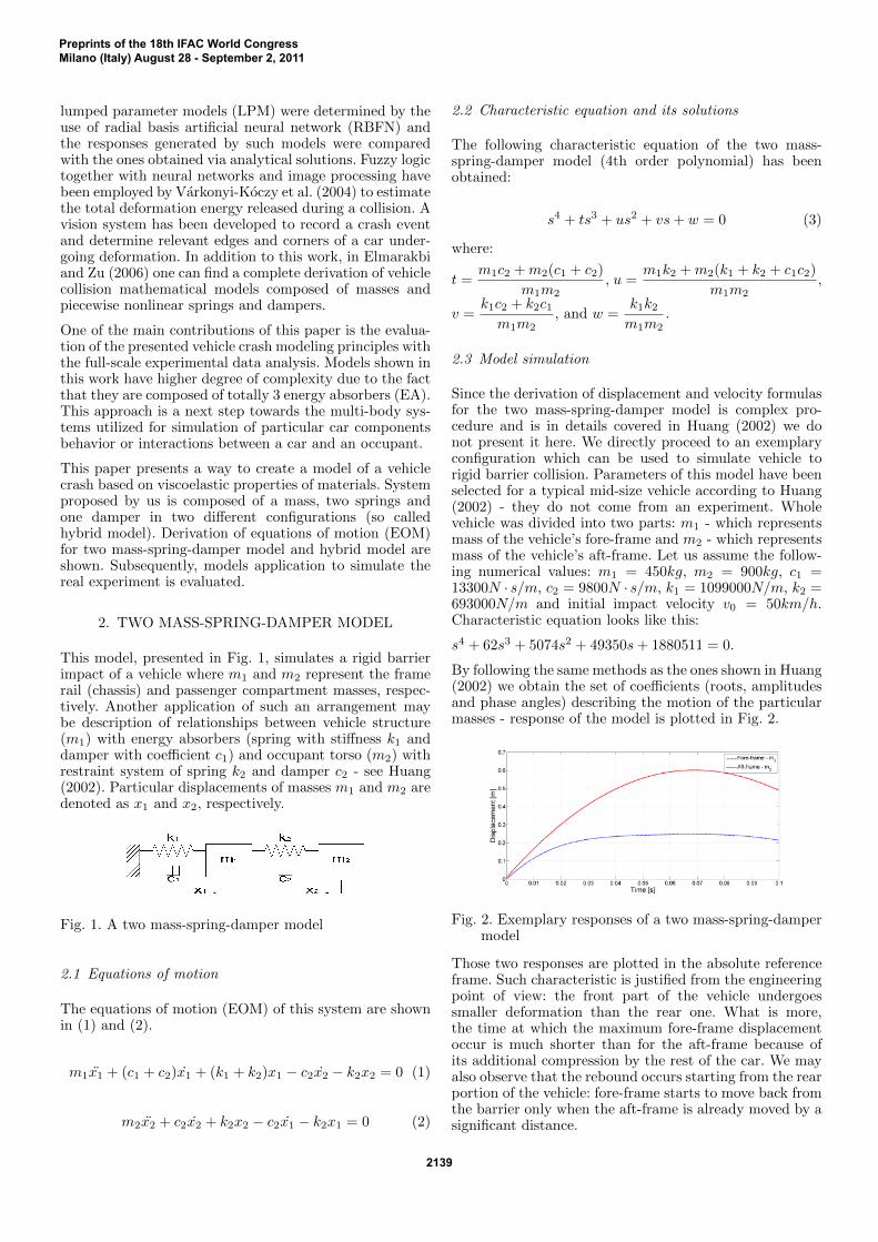
This model, presented in Fig. 1, simulates a rigid barrierimpact of a vehicle where m1 and m2 represent the framerail (chassis) and passenger compartment masses, respec-tively. Another application of such an arrangement maybe description of relationships between vehicle structure(m1) with energy absorbers (spring with stiffness k1 anddamper with coefficient c1) and occupant torso (m2) withrestraint system of spring k2 and damper c2 - see Huang(2002). Particular displacements of masses m1 and m2 aredenoted as x1 and x2, respectively.

Fig. 1. A two mass-spring-damper model

2.1 Equations of motion

The equations of motion (EOM) of this system are shownin (1) and (2).

m1x1 + (c1 + c2)x1 + (k1 + k2)x1 − c2x2 − k2x2 = 0 (1)

m2x2 + c2x2 + k2x2 − c2x1 − k2x1 = 0 (2)

2.2 Characteristic equation and its solutions

The following characteristic equation of the two mass-spring-damper model (4th order polynomial) has beenobtained:

s4 + ts3 + us2 + vs+ w = 0 (3)

where:

t =m1c2 +m2(c1 + c2)

m1m2, u =

m1k2 +m2(k1 + k2 + c1c2)

m1m2,

v =k1c2 + k2c1m1m2

, and w =k1k2m1m2

.

2.3 Model simulation

Since the derivation of displacement and velocity formulasfor the two mass-spring-damper model is complex pro-cedure and is in details covered in Huang (2002) we donot present it here. We directly proceed to an exemplaryconfiguration which can be used to simulate vehicle torigid barrier collision. Parameters of this model have beenselected for a typical mid-size vehicle according to Huang(2002) - they do not come from an experiment. Wholevehicle was divided into two parts: m1 - which representsmass of the vehicle’s fore-frame and m2 - which representsmass of the vehicle’s aft-frame. Let us assume the follow-ing numerical values: m1 = 450kg, m2 = 900kg, c1 =13300N · s/m, c2 = 9800N · s/m, k1 = 1099000N/m, k2 =693000N/m and initial impact velocity v0 = 50km/h.Characteristic equation looks like this:

s4 + 62s3 + 5074s2 + 49350s+ 1880511 = 0.

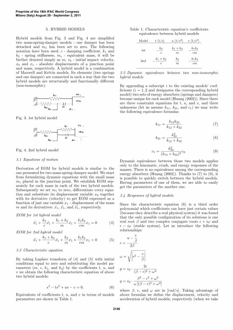
By following the same methods as the ones shown in Huang(2002) we obtain the set of coefficients (roots, amplitudesand phase angles) describing the motion of the particularmasses - response of the model is plotted in Fig. 2.

Fig. 2. Exemplary responses of a two mass-spring-dampermodel

Those two responses are plotted in the absolute referenceframe. Such characteristic is justified from the engineeringpoint of view: the front part of the vehicle undergoessmaller deformation than the rear one. What is more,the time at which the maximum fore-frame displacementoccur is much shorter than for the aft-frame because ofits additional compression by the rest of the car. We mayalso observe that the rebound occurs starting from the rearportion of the vehicle: fore-frame starts to move back fromthe barrier only when the aft-frame is already moved by asignificant distance.

Preprints of the 18th IFAC World CongressMilano (Italy) August 28 - September 2, 2011

2139

3. HYBRID MODELS

Hybrid models from Fig. 3 and Fig. 4 are simplifiedtwo mass-spring-damper models - one damper has beendetached and m1 has been set to zero. The followingnotation have been used: c - damping coefficient, k1 andk2 - spring stiffnesses, me - equivalent mass, it will befurther denoted simply as m, v0 - initial impact velocity,x0 and x1 - absolute displacements of a junction pointand mass, respectively. A hybrid model is a combinationof Maxwell and Kelvin models. Its elements (two springsand one damper) are connected in such a way that the twohybrid models are structurally and functionally different(non-isomorphic).

Fig. 3. 1st hybrid model

Fig. 4. 2nd hybrid model

3.1 Equations of motion

Derivation of EOM for hybrid models is similar to theone presented for two mass-spring-damper model. We startfrom formulating dynamic equations with the small massm1 placed in the junction point. We establish EOM sep-arately for each mass in each of the two hybrid models.Subsequently we set m1 to zero, differentiate every equa-tion and substitute its displacement variable x0 togetherwith its derivative (velocity) to get EOM expressed as afunction of just one variable x1 - displacement of the massm and its derivatives: x1, x1, and

...x1, respectively.

EOM for 1st hybrid model

...x1 +

k2cx1 +

k1 + k2m

x1 +k1k2cm

x1 = 0 (4)

EOM for 2nd hybrid model

...x1 +

k1 + k2c

x1 +k2mx1 +

k1k2cm

x1 = 0 (5)

3.2 Characteristic equation

By taking Laplace transform of (4) and (5) with initialconditions equal to zero and substituting the model pa-rameters (m, c, k1, and k2) by the coefficients t, u, andv we obtain the following characteristic equation of abovetwo hybrid models:

s3 − ts2 + us− v = 0. (6)

Equivalents of coefficients t, u, and v in terms of modelsparameters are shown in Table 1.

Table 1. Characteristic equation’s coefficientsequivalence between hybrid models

Model t [1/s] u [1/s2] v [1/s3]

1st −k2

c

k1 + k2

m−k1k2

cm

2nd −k1 + k2

c

k2

m−k1k2

cm

3.3 Dynamic equivalence between two non-isomorphichybrid models

By appending a subscript i to the existing models’ coef-ficients (i = 1, 2 and designates the corresponding hybridmodel) two sets of energy absorbers (springs and dampers)become unique for each model (Huang (2002)). Since thereare three constraint equations for t, u, and v, and threeunknowns (let us assume k11, k21, and c1) we may writethe following equivalence formulas:

k11 =k12k22k12 + k22

(7)

k21 =k222

k12 + k22(8)

c1 =k222

(k12 + k22)2c2. (9)

Dynamic equivalence between those two models appliesonly to the kinematic, crush, and energy responses of themasses. There is no equivalence among the correspondingenergy absorbers (Huang (2002)). Thanks to (7) to (9), itis possible to quickly switch between the hybrid models.Having parameters of one of them, we are able to easilyget the parameters of the another one.

3.4 Responses of hybrid models

Since the characteristic equation (6) is a third orderpolynomial which coefficients can have just certain values(because they describe a real physical system) it was foundthat the only possible configuration of its solutions is onereal root β and two complex conjugate roots ε + iω andε − iω (stable system). Let us introduce the followingrelationships:

ε =

u− v

β

2β

ω =

√∣∣∣∣ε2 − v

β

∣∣∣∣p = v0 ·

2ε

(β − ε)2 + ω2

q = v0 ·β2 − ε2 + ω2

ω [(β − ε)2 + ω2]

where β, ε, and ω are in [rad/s]. Taking advantage ofabove formulas we define the displacement, velocity andacceleration of hybrid models, respectively (when we take

Preprints of the 18th IFAC World CongressMilano (Italy) August 28 - September 2, 2011

2140

into account initial conditions at t = 0: x1 = 0, x1 = v0,and x1 = 0 we will de facto obtain a particular solution forthird order differential equation - EOM of hybrid model -and its two derivatives):

α = −peβt + eεt(p cosωt+ q sinωt) (10)

α = −pβeβt + eεt[ε(p cosωt+ q sinωt)−ω(p sinωt− q cosωt)]

(11)

α = −pβ2eβt + eεt[(ε2 − ω2)(p cosωt+ q sinωt)−2εω(p sinωt− q cosωt].

(12)

4. EXPERIMENT DESCRIPTION

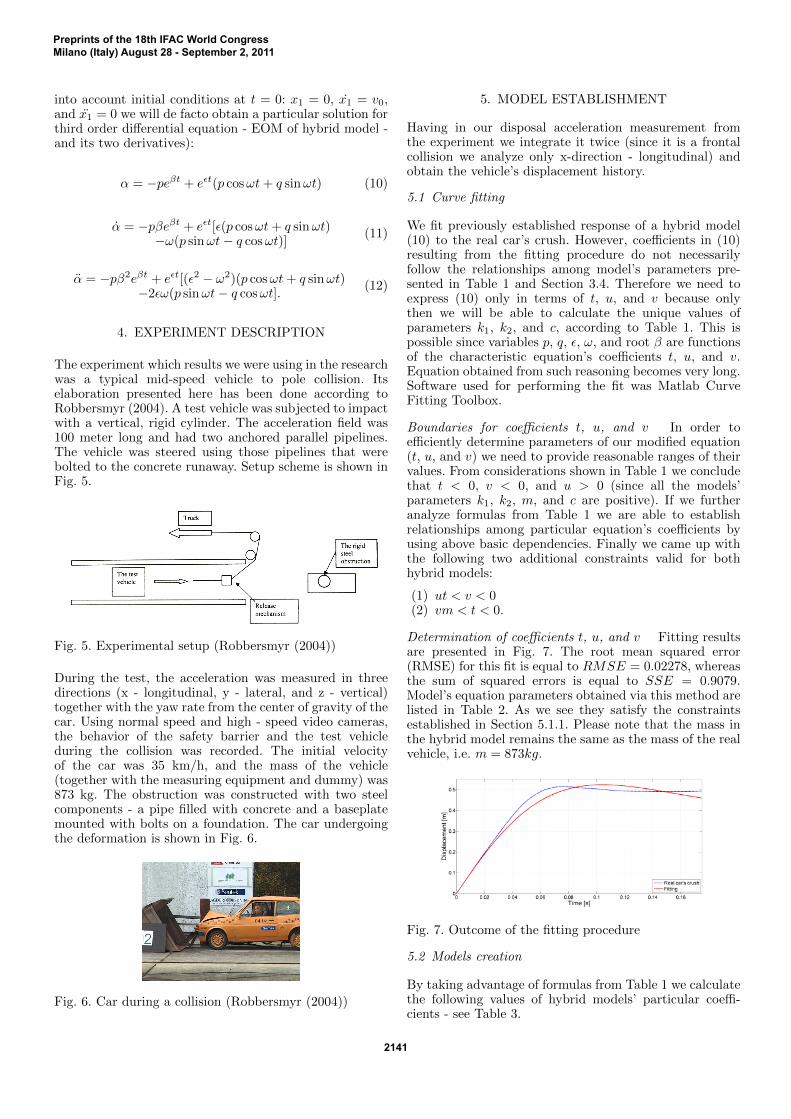
The experiment which results we were using in the researchwas a typical mid-speed vehicle to pole collision. Itselaboration presented here has been done according toRobbersmyr (2004). A test vehicle was subjected to impactwith a vertical, rigid cylinder. The acceleration field was100 meter long and had two anchored parallel pipelines.The vehicle was steered using those pipelines that werebolted to the concrete runaway. Setup scheme is shown inFig. 5.

Fig. 5. Experimental setup (Robbersmyr (2004))

During the test, the acceleration was measured in threedirections (x - longitudinal, y - lateral, and z - vertical)together with the yaw rate from the center of gravity of thecar. Using normal speed and high - speed video cameras,the behavior of the safety barrier and the test vehicleduring the collision was recorded. The initial velocityof the car was 35 km/h, and the mass of the vehicle(together with the measuring equipment and dummy) was873 kg. The obstruction was constructed with two steelcomponents - a pipe filled with concrete and a baseplatemounted with bolts on a foundation. The car undergoingthe deformation is shown in Fig. 6.

Fig. 6. Car during a collision (Robbersmyr (2004))

5. MODEL ESTABLISHMENT

Having in our disposal acceleration measurement fromthe experiment we integrate it twice (since it is a frontalcollision we analyze only x-direction - longitudinal) andobtain the vehicle’s displacement history.

5.1 Curve fitting

We fit previously established response of a hybrid model(10) to the real car’s crush. However, coefficients in (10)resulting from the fitting procedure do not necessarilyfollow the relationships among model’s parameters pre-sented in Table 1 and Section 3.4. Therefore we need toexpress (10) only in terms of t, u, and v because onlythen we will be able to calculate the unique values ofparameters k1, k2, and c, according to Table 1. This ispossible since variables p, q, ε, ω, and root β are functionsof the characteristic equation’s coefficients t, u, and v.Equation obtained from such reasoning becomes very long.Software used for performing the fit was Matlab CurveFitting Toolbox.

Boundaries for coefficients t, u, and v In order toefficiently determine parameters of our modified equation(t, u, and v) we need to provide reasonable ranges of theirvalues. From considerations shown in Table 1 we concludethat t < 0, v < 0, and u > 0 (since all the models’parameters k1, k2, m, and c are positive). If we furtheranalyze formulas from Table 1 we are able to establishrelationships among particular equation’s coefficients byusing above basic dependencies. Finally we came up withthe following two additional constraints valid for bothhybrid models:

(1) ut < v < 0(2) vm < t < 0.

Determination of coefficients t, u, and v Fitting resultsare presented in Fig. 7. The root mean squared error(RMSE) for this fit is equal to RMSE = 0.02278, whereasthe sum of squared errors is equal to SSE = 0.9079.Model’s equation parameters obtained via this method arelisted in Table 2. As we see they satisfy the constraintsestablished in Section 5.1.1. Please note that the mass inthe hybrid model remains the same as the mass of the realvehicle, i.e. m = 873kg.

Fig. 7. Outcome of the fitting procedure

5.2 Models creation

By taking advantage of formulas from Table 1 we calculatethe following values of hybrid models’ particular coeffi-cients - see Table 3.

Preprints of the 18th IFAC World CongressMilano (Italy) August 28 - September 2, 2011

2141

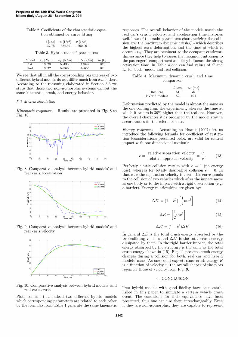
Table 2. Coefficients of the characteristic equa-tion obtained by curve fitting

t [1/s] u [1/s2] v [1/s3]

-32.75 684.60 -500.00

Table 3. Hybrid models’ parameters

Model k1 [N/m] k2 [N/m] c [N · s/m] m [kg]

1st 13328 584330 17842 8732nd 13632 597660 18665 873

We see that all in all the corresponding parameters of twodifferent hybrid models do not differ much from each other.According to the reasoning elaborated in Section 3.3 westate that those two non-isomorphic systems exhibit thesame kinematic, crush, and energy behavior.

5.3 Models simulation

Kinematic responses Results are presented in Fig. 8 toFig. 10.

Fig. 8. Comparative analysis between hybrid models’ andreal car’s acceleration

Fig. 9. Comparative analysis between hybrid models’ andreal car’s velocity

Fig. 10. Comparative analysis between hybrid models’ andreal car’s crush

Plots confirm that indeed two different hybrid modelswhich corresponding parameters are related to each otherby the formulas from Table 1 generate the same kinematic

responses. The overall behavior of the models match thereal car’s crush, velocity, and acceleration time historieswell. Two of the main parameters characterizing the colli-sion are: the maximum dynamic crush C - which describesthe highest car’s deformation, and the time at which itoccurs - tm. They are pertinent to the occupant crashwor-thiness since they help to assess the maximum intrusion tothe passenger’s compartment and they influence the airbagactivation time. In Table 4 one can find values of C andtm for both: model and real collision.

Table 4. Maximum dynamic crush and timecomparison

C [cm] tm [ms]

Real car 51 76Hybrid models 52 104

Deformation predicted by the model is almost the same asthe one coming from the experiment, whereas the time atwhich it occurs is 36% higher than the real one. However,the overall characteristics produced by the model stay inaccordance with the reference ones.

Energy responses According to Huang (2002) let usintroduce the following formula for coefficient of restitu-tion (considerations presented below are valid for centralimpact with one dimensional motion):

e =relative separation velocity

relative approach velocity=v′

v. (13)

Perfectly elastic collision results with e = 1 (no energyloss), whereas for totally dissipative collision e = 0. Inthat case the separation velocity is zero - this correspondsto the collision of two vehicles which after the impact moveas one body or to the impact with a rigid obstruction (e.g.a barrier). Energy relationships are given by:

∆E′ = (1− e2)

[1

2mv2

](14)

∆E =

[1

2mv2

](15)

∆E′ = (1− e2)∆E. (16)

In general ∆E is the total crush energy absorbed by thetwo colliding vehicles and ∆E′ is the total crush energydissipated by them. In the rigid barrier impact, the totalenergy absorbed by the structure is the same as the totalcrush energy shown in (15). Fig. 11 presents crush energychanges during a collision for both: real car and hybridmodels’ mass. As one could expect, since crush energy Eis a function of velocity v, the overall shapes of the plotsresemble those of velocity from Fig. 9.

6. CONCLUSION

Two hybrid models with good fidelity have been estab-lished in this paper to simulate a certain vehicle crashevent. The conditions for their equivalence have beenpresented, thus one can use them interchangeably. Evenif they are non-isomorphic, they are capable to represent

Preprints of the 18th IFAC World CongressMilano (Italy) August 28 - September 2, 2011

2142

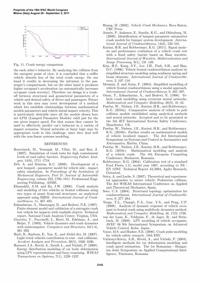
Fig. 11. Crush energy comparison

the each other’s behavior. By analyzing the collision fromthe energetic point of view, it is concluded that a stiffervehicle absorbs less of the total crush energy. On onehand it results in decreasing the intrusion to the pas-senger’s compartment, but on the other hand it produceshigher occupant’s acceleration (so automatically increasesoccupant crash severity). Therefore car design is a trade-off between structural and geometrical parameters of avehicle and desired safety of driver and passengers. Futurework in this area may cover development of a methodwhich lets establish relationships between mathematicalmodels parameters and vehicle initial impact velocity. Thisis particularly desirable since all the models shown hereare LPM (Lumped Parameter Models) valid just for theone given impact speed. For that reason they cannot beused to effectively predict car’s behavior in a variety ofimpact scenarios. Neural networks or fuzzy logic may beappropriate tools in this challenge, since they deal wellwith the non-linear systems modeling.

REFERENCES

Borovinsek, M., Vesenjak, M., Ulbin, M., and Ren, Z.(2007). Simulation of crash tests for high containmentlevels of road safety barriers. Engineering Failure Anal-ysis, 14(8), 1711–1718.

Deb, A. and Srinivas, K.C. (2008). Development of anew lumped - parameter model for vehicle side - impactsafety simulation. In Proceedings of the Institution ofMechanical Engineers, Part D: Journal of AutomobileEngineering, volume 222, 1793–1811. Professional Engi-neering Publishing. ASME.

Elmarakbi, A.M. and Zu, J.W. (2006). Crash analysisand modeling of two vehicles in frontal collisions usingtwo types of smart front-end structures: an analyticalapproach using IHBM. International Journal of Crash-worthiness, 11, 467–483.

Eskandarian, A., Marzougui, D., and Bedewi, N.E. (1997).Finite element model and validation of a surrogate crashtest vehicle for impacts with roadside objects. Technicalreport, National Crash Analysis Center, Virginia, USA.

Giavotto, V., Puccinelli, L., Borri, M., Edelman, A., andHeijer, T. (1983). Vehicle dynamics and crash dynamicswith minicomputer. Computers and Structures, 16(1-4),381–393.

Harb, R., Radwan, E., Yan, X., and Abdel-Aty, M. (2007).Light truck vehicles contribution to rear - end collisions.Accident Analysis and Prevention, 39(5), 1026–1036.

Harmati, I.A., Rovid, A., Szeidl, L., and Varlaki, P. (2008).Energy distribution modeling of car body deformationusing LPV representations and fuzzy reasoning. WSEASTransactions on Systems, 7(1), 1228–1237.

Huang, M. (2002). Vehicle Crash Mechanics. Boca Raton,CRC Press.

Jonsen, P., Isaksson, E., Sundin, K.G., and Oldenburg, M.(2009). Identification of lumped parameter automotivecrash models for bumper system development. Interna-tional Journal of Crashworthiness, 14(6), 533–541.

Karimi, H.R. and Robbersmyr, K.G. (2011). Signal analy-sis and performance evaluation of a vehicle crash testwith a fixed safety barrier based on Haar wavelets.International Journal of Wavelets, Multiresoloution andImage Processing, 9(1), 131–149.

Kim, H.S., Kang, S.Y., Lee, I.H., Park, S.H., and Han,D.C. (1996). Vehicle frontal crashworthiness analysis bysimplified structure modeling using nonlinear spring andbeam elements. International Journal of Crashworthi-ness, 2, 107–118.

Moumni, Z. and Axisa, F. (2004). Simplified modelling ofvehicle frontal crashworthiness using a modal approach.International Journal of Crashworthiness, 9, 285–297.

Omar, T., Eskandarian, A., and Bedewi, N. (1998). Ve-hicle crash modelling using recurrent neural networks.Mathematical and Computer Modelling, 28(9), 31–42.

Pawlus, W., Nielsen, J.E., Karimi, H.R., and Robbersmyr,K.G. (2010a). Comparative analysis of vehicle to polecollision models established using analytical methodsand neural networks. Accepted and to be presented atthe 5th IET International System Safety Conference,Manchester, UK.

Pawlus, W., Nielsen, J.E., Karimi, H.R., and Robbersmyr,K.G. (2010b). Further results on mathematical modelsof vehicle localized impact. The 3rd InternationalSymposium on Systems and Control in Aeronautics andAstronautics, Harbin, China.

Pawlus, W., Nielsen, J.E., Karimi, H.R., and Robbersmyr,K.G. (2010c). Mathematical modeling and analysisof a vehicle crash. The 4th European ComputingConference, Bucharest, Romania.

Robbersmyr, K.G. (2004). Calibration test of a standardFord Fiesta 1.1l, model year 1987, according to NS -EN 12767. Technical Report 43/2004, Agder Research,Grimstad.

Soica, A. and Lache, S. (2007). Theoretical and experimen-tal approaches to motor vehicle: Pedestrian collision.The 3rd WSEAS International Conference on Appliedand Theoretcial Mechanics, Spain.

Soto, C.A. (2004). Structural topology optimization forcrashworthiness. International Journal of Crashworthi-ness, 9, 277–284.

Tenga, T.L., Changb, F.A., Liuc, Y.S., and Peng, C.P.(2008). Analysis of dynamic response of vehicle occu-pant in frontal crash using multibody dynamics method.Mathematical and Computer Modelling, 48, 1724–1736.

van der Laan, E., Veldpaus, F., de Jager, B., and Stein-buch, M. (2008). LPV modeling of vehicle occupants.AVEC 08 9th International Symposium on AdvancedVehicle Control, Kobe, Japan.

Varat, M.S. and Husher, S.E. (2000). Crash pulse modelingfor vehicle safety research. 18th ESV.

Varkonyi-Koczy, A.R., Rovid, A., and Varlaki, P. (2004).Intelligent methods for car deformation modeling andcrash speed estimation. The 1st Romanian - Hungar-ian Joint Symposium on Applied Computational Intel-ligence, Timisoara, Romania.

Preprints of the 18th IFAC World CongressMilano (Italy) August 28 - September 2, 2011

2143