The Optimized QuaDRiGa Wi-Fi Channel Model · The Optimized QuaDRiGa Wi-Fi Channel Model ......

51

International Journal of

Science and Engineering Investigations vol. 4, issue 44, September 2015

ISSN: 2251-8843

The Optimized QuaDRiGa Wi-Fi Channel Model

Mohammad E. Ranjkesh1, Ali Akbar Khazaei

2

1Department of Telecommunication, Khavaran Institute of Higher Education, Mashhad, Iran

2Department of Electrical Engineering, Mashhad Branch Islamic Azad University, Mashhad, Iran

([email protected], [email protected], [email protected], [email protected])

Abstract- This paper propose an optimal Wi-Fi channel model

by definition second order environment interactions

computation in the quasi deterministic radio channel generator

(QuaDRiGa) model. This is an undeniable truth in some

environments especially indoor environments, dispersive signal

has many interactions with its environs. Hence, in addition to

line of sight (LOS) interactions, non-line of sight (NLOS)

interactions has a significant impact on radio channel modeling

process. In the previous QuaDRiGa model, only two kind of

interactions considered which named LOS and single

interaction clusters (NLOS_SICs), but, for the new optimized

channel model also, intervened one kind of non-line of sight

multiple interaction clusters (NLOS_MICs) known as non-line

of sight twin interaction clusters (NLOS_TICs). Therefore,

more details of departure and arrival angles, delay spread and

powers are changed in the channel coefficient computations.

Summary, when the clusters formed by the means of

parameterizing large-scale parameter (LSP), the cluster types

recognition approach used to determining clusters type and

then for each of them, different methods used to calculate

channel parameters. Finally, experimental result and numerical

analysis (e.g. shadow fading, K factor delay spread) show that

the proposed channel model is able to serve as a more accurate

design framework for Wi-Fi Multiple input-Multiple output

(MIMO) channel model and have a better performance than

previous QuaDRiGa in the channel coefficient estimation .

Keywords- WiFi channel model, QuaDRiGa, MIMO, Twin

interaction cluster (TIC), LSP

I. INTRODUCTION

Channel models are important tools to evaluate the performance of new concepts in wireless communication. There is a tradeoff between complexity and accuracy of channel modeling methods and different wireless scenarios have different complexity too [1]. In Wi-Fi scenarios especially in indoor situations, dispersive signal limited by shadowing or blocking objects are located in the direct path. This aspect increases its modeling complexity. To consider these limitations and surveying signal interactions, Channel models such as the 3GPP spatial channel model (SCM) [1, 2], the Wireless World Initiative for New Radio (WINNER) model [3, 4] and the European Cooperation in Science and Technology

(COST) 273/2100 channel model [5, 6] are reliable tools. These channel models developed and improved over the time. One of the newest channel modeling methods is the QuaDRiGa. The QuaDRiGa channel model [7] to [9] is a promotion of the WINNER channel model. The key aspects of QuaDRiGa are geo-correlated parameters maps, three dimensional antenna characteristics, a novel geometric polarization model, continuous drifting of small and large scale effects along user equipment (UE) movement, non-constant velocities as well as transitions between varying propagation scenario [10]. This model combines the advantages of deterministic and statistical channel modeling approach for MIMO systems [10]. Based on empirical statistics a random scenario is generated. Within that scenario, behavior of the model is deterministic. Thus, the QuaDRiGa consists of two steps: at first stochastic part generates the LSP and then, random positions of scattering clusters calculated [8]. After calculation of scattering clusters positions, assumed all clusters deemed two kinds: LOS and NLOS_SICs, then, evolution based on this ideas presented [7, 8]. Accordingly, NLOS_MICs ignored and this matter reduce channel modeling accuracy.

In this paper used the QuaDRiGa channel model and in addition to prepare a 3D Wi-Fi channel model with time evolution feature, one of the most effective multiple interaction component of the NLOS signal known as NLOS_TICs considered and its delays, powers, angle of arrival and angle of departure are involved. Recognition of cluster's type come after cluster formed. Consequently, by the means of this concept channel model's accuracy increased. A reference implementation of QuaDRiGa in MATLAB is available as open source [9] used and extended to simulation and extracting results.

The paper is organized as follows. Section 2 describes an overview of the QuaDRiGa model. Section 3 illustrates a cluster identification method. Section 4 describes O-QuaDRiGa Wi-Fi channel model by combination of sections 2 and 3. Section 5 shows results discussion and compares the results from both model and measurement data. Section 6 concludes the paper.

II. THE QUADRIGA MODEL BASICS

The QuaDRiGa channel model follows a geometry-based stochastic channel modeling approach, which allows creation

International Journal of Science and Engineering Investigations, Volume 4, Issue 44, September2015 52

www.IJSEI.com Paper ID: 44415-09 ISSN: 2251-8843

an arbitrary double directional radio channel. As mentioned, it can be considered as an extension of the WINNER model. So, large parts of QuaDRiGa are similar to this model. This model's main structure generally divided into the following parts:

Scenario definition

Large scale parameters (LSPs) configuration

Drifting

Transition between segments

A. Scenario definition

In the QuaDRiGa channel modeling simulation process, user should be setup some parameters of signal diffusion environment, known as scenario definition. For example: positioning of all transmitters, choosing a trajectory for all user equipment (UEs), antenna configuration for transmitters and receivers, and propagation conditions (e.g. carrier frequency, environment type such as urban, rural, LOS and NLOS, light speed, etc.) categorized in this part. As regards QuaDRiGa is intended for long term observation, the environment types might change along the UEs movement's trajectory. A method to keep track of propagation conditions which used in QuaDRiGa is to generate parameter maps for every environment type and for the whole area which is occupied by the trajectories of UEs [8].(*Note: Defined scenario for both the QuaDRiGa and the O-QuaDRiGa is Wi-Fi propagation scenario.)

B. Large scale parameters (LSPs) configuration

The positions of the scattering clusters determined based on grouping LSPs. LSPs listed in the following:

1) RMS delay spread (DS).

2) Ricean K-factor (KF).

3) Shadow fading (SF).

4) Azimuth spread of departure (ASD).

5) Azimuth spread of arrival (ASA).

6) Elevation spread of departure (ESD).

7) Elevation spread of arrival (ESA).

Distribution properties of these parameters directly obtained from measurement data (e.g. [3, 4], [11]-[13]). By these distributions, the LSP maps calculated and drawn. If some MTs or segments are close to each other, their LSPs will be correlated and can have similar propagation conditions. A 2D maps used to model this correlation comes from [14]. The maps initialized with values obtained from an independent and identically distributed (i.i.d.) zero-mean Gaussian random process with desired variance. After that, pixels filtered to obtain the desired autocorrelation function. This function modeled by an exponential decay [7]:

ρ(d) =

(1)

Which, γ is the autocorrelation distance and its

significance well known and explained in [15].

Then, in contrast to [14], the maps filtered in the diagonal direction as well to get a smooth evolution of the values along the MT trajectory [8]. More details come in the following subsections:

1) Initial Delays and Powers of Cluster: Initial delays are drawn randomly from a scenario-dependent delay distribution as

l[1]

= - rτ στ ln(Xl) (2)

Where Xl uni (0, 1) is an uniformly distributed random variable having values between 0 and 1, στ is the initial DS from the map and rτ is a proportionality factor [3]. Because στ is influenced by both the delays l and the powers Pl ; rτ introduced and calculated from measurement data. After this step, delays must be normalized such that the first delay is zero and then they are sorted:

l[2]

= sort { l[1]

- min ( l[1]

) } (3)

he cluster powers are drawn from a single slope e ponential power-delay profile ( ) depending on the στ and a random component l ( 0, ζ

2) [3]. The ζ is a

coefficient which dependent on scenario and emulating an additional shadowing process. In the following equation shown how it is obtained from measurements:

l[1]

= exp (

)

(4)

The first cluster's power is further scaled according to the initial KF from the map and cluster powers are normalized so that their sum power is one:

1[2]

= K ∑ ; 2...l

[2] = 2...l

[1] and l

= l

[2]

∑ (5)

At last, the influence of the KF on the DS corrected, which has changed due to the scaling. The DS after applying (5) is

calculated using (9) with Pi set to one and named

[8].

στi = √

∑

(

∑

)

(6)

In this equation, is the interval length corresponds to the time resolution of our measurement system, which is 54.5 ns at 18.36 MHz bandwidth.

Finally, with στ being the initial from the map, cluster delays note

τl =

(7)

1) Ricean K-factor (KF) and Shadow fading (SF) The KF and the SF obtained from the map by an

interpolation of the surrounding pixels at the position of sth

snapshot [8, 16]. The KF at the initial position is already included due to the scaling in (5). Then, It must be take into account and scale the power accordingly.

gr,t,l,s =

. {√

(8)



= √ . √ (

)

and are the interpolated values for the KF and

the SF from the map, is the KF at the initial position,

, is the path gain at the MT position (9) and is the

power of the LOS cluster from (5).

PG[dB]

= -A1 . 10 log10 d[m] - A2 (9)

The PG scales with the logarithm of the distance d (in meter) between Satellite and terminal. In (9), A1 , A2 are coefficients depends on scenario and typically determined by measurements. A1 often varies between 2 and 4 and depending on the propagation conditions, the BS height and other factors.

2) Departure and Arrival angles In the QuaDRiGa, four angles calculated for each cluster.

Calculation of the azimuth angle of departure (Ao , φd) and

the azimuth angle of arrival (AoA, φa) which used in WINNER

2D model and the elevation angle of departure (EoD, ϴd) and

the elevation angle of arrival (EoA, ϴa) done in this model.

These angles have the same calculation method but thier angular spreads σφ are different together. By using σφ

representative for , , , in the follow and assume

a wrapped Gaussian distribution for the power angular spectrum of all clusters[3, 17]:

(φ) =

√ (

) (10)

Since (10) assumes a continuous spectrum, whereas the channel model uses discrete paths, its needed to correct the variance by a function Cφ(L,K). This function ensures that the input variance σφ is correctly reflected in the generated angles [8].

The angles φl obtained by first normalizing the power angular spectrum, so that its maximum has unit power. By

omitting the scaling factor (

√ and normalizing the path

powers Pl in (5) so that the strongest peak with unit power corresponds to an angle φ = 0. ther paths get relative departure or arrival angles depending on their power :

φl [1]

=

. √

(11)

The value σφ is measured in radians. Next, two random variables created, Xl and Yl. Xl {-1, 1}is the positive or negative sign and Yl N( 0, 0.01

. σφ

2) introduces a random

variation of the angle. Then the following term calculated:

φl [2]

= Xl . φl [1]

+ Yl (12)

By comparing each path power (Pl) with strongest peak, if Pl to be small, its angle might e ceed ±π. Hence, wrapped around the unit circle by following operation:

φl [3]

= (φl [2]

+ π mod 2π ) - π (13)

For elevation spreads, the possible elevation angles range goes from -π/2 to π/2. Equation (14) correct values of φl

[3]

which out of this range:

φl [4]

=

{

|

|

(14)

The position of transmitters (Tx) and receiver (Rx) and

thereby the angles of LOS component are deterministic. Then in the next correction used (15):

φl [5]

= φl [4]

- φ1[4]

+ φ LOS

(15)

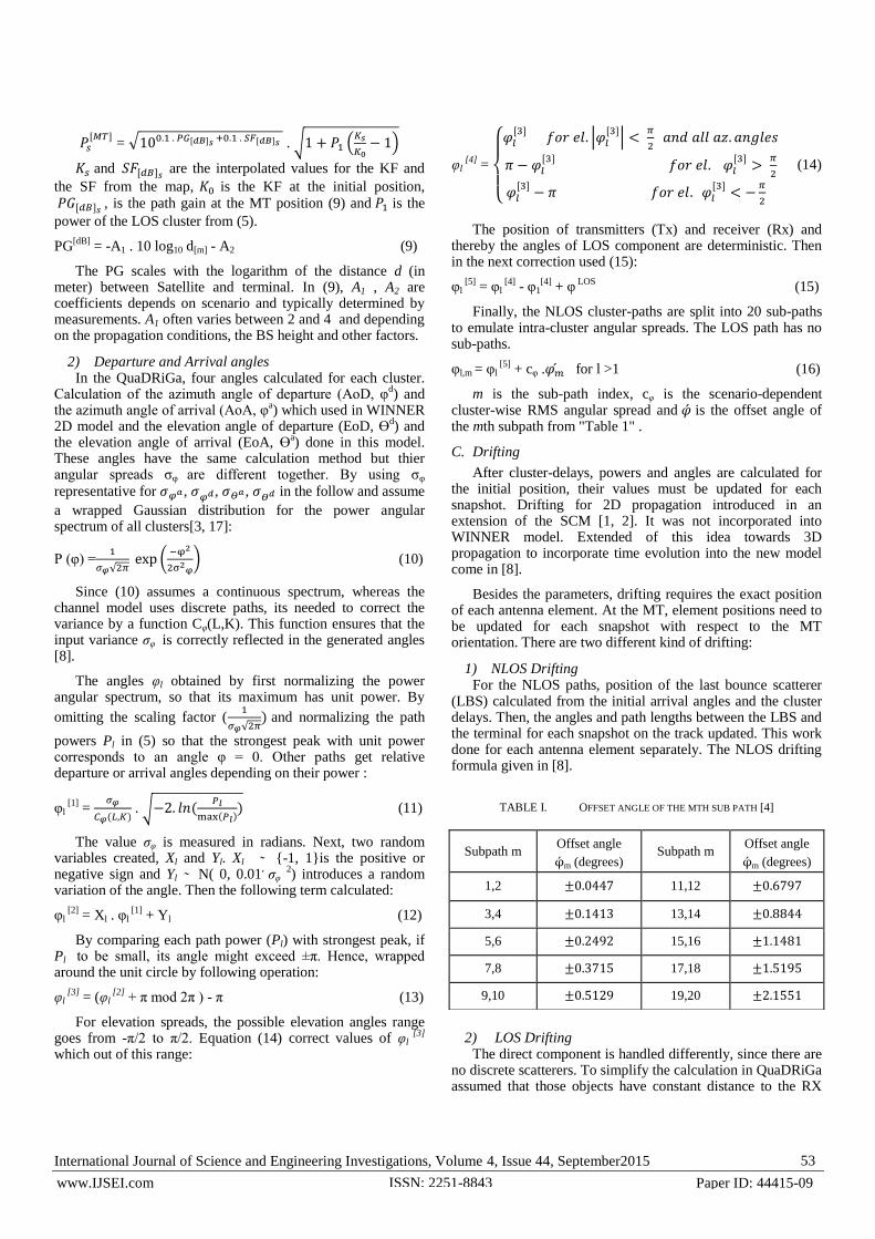
Finally, the NLOS cluster-paths are split into 20 sub-paths to emulate intra-cluster angular spreads. The LOS path has no sub-paths.

φl,m = φl [5]

+ cφ . for l >1 (16)

m is the sub-path index, cφ is the scenario-dependent cluster-wise RMS angular spread and is the offset angle of the mth subpath from "Table 1" .

C. Drifting

After cluster-delays, powers and angles are calculated for the initial position, their values must be updated for each snapshot. Drifting for 2D propagation introduced in an extension of the SCM [1, 2]. It was not incorporated into WINNER model. Extended of this idea towards 3D propagation to incorporate time evolution into the new model come in [8].

Besides the parameters, drifting requires the exact position of each antenna element. At the MT, element positions need to be updated for each snapshot with respect to the MT orientation. There are two different kind of drifting:

1) NLOS Drifting For the NLOS paths, position of the last bounce scatterer

(LBS) calculated from the initial arrival angles and the cluster delays. Then, the angles and path lengths between the LBS and the terminal for each snapshot on the track updated. This work done for each antenna element separately. The NLOS drifting formula given in [8].

TABLE I. OFFSET ANGLE OF THE MTH SUB PATH [4]

2) LOS Drifting The direct component is handled differently, since there are

no discrete scatterers. To simplify the calculation in QuaDRiGa assumed that those objects have constant distance to the RX

Subpath m Offset angle

m (degrees) Subpath m

Offset angle

m (degrees)

1,2 11,12

3,4 13,14

5,6 15,16

7,8 17,18

9,10 19,20



and are only separated by their angular distributions. Calculation of the LOS drifting given in [8].

D. Transition between segments

A segment is a part of receivers trajectory which the channel assumed wide sense stationary (WSS) in it. In previous sections, all calculation related to each segment of the MT trajectory independently. This step combine those segments into a long, named merging. The idea comes from the WINNER II model [3]. However, it was neither implemented nor tested.

The life time of a scattering cluster is confined within the combined length of two adjacent segments. The power of clusters from the old segment is ramped down and the power of new clusters is ramped up within the overlapping region of the two segments. Hence, this process describes the birth and death of clusters around the trajectory. Outside the overlapping region, all clusters of the segment are active. We further split the overlapping region into subintervals to keep the computational overhead low.

During each subinterval, one old cluster ramps down and one new cluster ramps up. Then QuaDRiGa model the power ramps by a squared sine function:

= sin2 (

) (17)

In (17), is the linear ramp ranging from 0 to 1, is the corresponding sine-shaped ramp with a constant slope at the beginning and the end. This prevents inconsistencies at the edges of the sub intervals. If both segments have a different number of clusters, the ramp is stretched over the whole overlapping area for clusters without a partner. For the LOS cluster, which is present in both segments, only power and phase adjusted [8]. To minimize the impact of the transition on the instantaneous values of the LSPs should be carefully mached together. In Fig. 1 shown how to transition between consecutive segments happen.

III. CLUSTERS IDENTIFICATION

To consistent performance evaluation, the channel models needed to be parameterized by multipath parameters based on measurements. It seems these parameters can be grouped into geometrically co-located paths, so called clusters [18].

Figure 1. Transition between consecutive segments

Figure 2. Different kind of clusters in wireless MIMO channel model: local

clusters ( green colour ), SICs ( violet colour), TICs ( blue colour ), LOS

component ( red colour)[20]

A. Different kind of clusters

There are three different kinds of clusters after initializing the propagation environment: (1) local clusters, (2) single interaction clusters (SICs), (3) multiple interaction clusters (MICs). Fig. 2 provide a schematic representation of these clusters [19- 21]. Their properties are reviewed in the following paragraph.

1) Local cluster: Around the MTs and around the BSs in

pico-cell or ad-hoc scenarios, local clusters will be found.

They always taken as single-bounced and are always active,

thus they contribute to the channel impulse response. Their

size is given by their delay spread specified in the model.

These clusters introduce an omnidirectional azimuth spread

around the respective station at low delay, which is frequently

observed in measurements [19].

2) Single interaction clusters: This kind of clusters

provide a single-bounce link between the BS and the MS

similar to local clusters. In macrocells, they are the dominant

mechanism, representing reflections of large building, hills,

etc. In microcells and picocells, single bounce scattering also

occurs through less frequently.

3) Multiple interaction clusters: Especially in picocells

and sometimes in microcell scenarios, they occurred. The

occurrence frequency of the MICs with respect to the SICs is

inversely proportional to the selection factor, Ksel, which

indicates the ratio between SICs and MICs. In macro-, micro-

and pico-cells scenarios this factor is set to 1, 0.5 and 0

respectively.

B. Identification Framework

In the following introduced a simple framework to contradistinction cluster type. This framework divided into three steps.

1) LOS component: In LOS scenarios, the location of LOS

component (which is also identified as cluster in the

measurements) can easily be identified from the

measurements using the delay, azimuth of departure and

azimuth of arrival.



Naturally, it should have stronger power than the surrounding clusters. After identifying its parameters, these clusters removed from the result set.

2) Local cluster: Clustering algorithms that include power

to identify clusters more accurately will naturally split up the

local cluster into multiple smaller ones. However, using the

knowledge of the BS and MS position, clusters contributing to

the local cluster can easily be identified. The local cluster around the MS is found at a distinct angle

seen from the BS, which can be obtained from the location information of MS and BS. These cluster seen wide-spread from the MS. The same identification method is used for the local cluster around the BS. After having identified all clusters in the result set that contribute to the local clusters, they are removed from the result set.

3) SICs and MICs: At first, distinguished whether a cluster

stems from single-bounce or multiple-bounce mechanisms

using the following method (see Fig. 3).

3-1. Determine the diameter of the cluster in space from its

delay spread as dc=3στ . c0, where c0 denotes the speed of light.

3-2. Determine the distance of the cluster from the BS and

from the MS by dBS/MS = dc /2tan(3σφB /M ). The associated

delay are defined as τBS/MS=dBS/MS/c0. The total delay of the

cluster is then described by τC = τC,BS + τC,MS + τC,link. The last

term describes the link delay of the cluster.

3-3. The link delay decides whether the cluster stems from a

single-bounce or double-bounce reflection by:

{

(18)

Where є is set close to zero. Estimation errors and errors in identifying clusters can be accounted for by a larger value of є. Note that it might sometimes happen that the link delay gets smaller than zero, which also evolves from the estimation variances of the path estimator or from the cluster identification [19].

Figure 3. Distinguishing between SICs and MICs: for ICs, τlink is close to

zero.

Fig. 4-1

Figure 4. Simplified overview of the modeling components used in

QuaDRiGa and O-QuaDRiGa

IV. OPTIMAL QUADRIGA CHANNEL MODEL (O-QUADRIGA)

IN WI-FI SCENARIOS

The QuaDRiGa modeling approach can be understood as a "statistical ray-tracing model", but unlike classical ray-tracing approach, it doesn't use an exact geometric representation of the environment and distributes the positions of the scattering clusters randomly. As shown in Fig. 4-1, in it, thought components only included delays and powers of NLOS_SICs and the LOS. Hence, NLOS_MICs ignored, and then thier delays and powers calculations do not have a high accuracy. In our modeling approach with attention to NLOS_MICs, modeling accuracy increased. Fig. 4-2 shows O-QuaDRiGa modeling components.

Impulse Response

Power

Signal

Delay

PLOS

PNLOS,Single-Cluster

PNLOS,Twin-Cluster

LOSƮ NLOS,S-CƮ NLOS,T-CƮ

Cluster seen from

BS

Cluster seen from

MS

τlin

k

dB

S dM

S

dC

dC

φB

S

φM

S

3σφB

S 3σφ

MS

BS

MS



So, new model operational process by attention to explained aspects introduced in the following three main steps:

A. Using the QuaDRiGA model steps till the clusters formed

For the new model all primary structures are similar to the QuaDRiGa. At first, the scenario parameters e.g. positioning of all transmitters, trajectory for all user equipment, antenna configuration of transmitters and receivers, and propagation conditions should be configured by the user. In the next step the LSP maps calculated and drawn by its measurment distributions and then, correlation between these parameters calculated too. Finally, the LSPs used to determine clusters initial delays and powers.

B. Identification and isolation of clusters

After the sub-section A, by using the introduced cluster identification method in section III, kind of clusters determined.

The LOS components are separated in the QuaDRiGa channel model. This kind of component directly used in the new model, too. For the O-QuaDriGa model, the local clusters like QuaDriGa, defined and examined similar to SICs. By the means of calculated delays in the previous part, and calculation of the link delays in the new model, discrimination of SICs and MICs will be done. In Fig. 5 shown all clusters of segments 2, 3, 6 and 11 which all of them are TICs.

C. Changing the calculation of angles and follow that, delays

and powers of clusters

After recognition cluster's type, SICs calculations done similar to pervious method and for the MICs changed angles, delays and powers calculation with some assumptions.

Assume, maximum numbers of interactions are two times, and more interactions because of high delay and low power do not examined. Then, by this definition MICs named TICs. In two clusters of the TIC assumed, nearer cluster into BS is first interaction cluster and the other is last interaction_cluster. After recognition of all first and last interaction clusters, all combination cases of them should be examined.

Figure 5. TICs in segments 2, 3, 6 and 11 with their centers, and Reciver

and Transmitter positions

Figure 6. Different combination of first mutation clusters and second mutation clusters in TICs conditions

(a)

(b)

Figure 7. (a) The QuaDRiGa model. (b) The O-QuaDRiGa model. Position

dependent delay spread of the Wi-Fi simulated track

For example as shown in Fig. 6 if the number of pair clusters tobe 3, total states which should be examined are 3

2

=9 states.

For all combination cases arrival and departure angles, delays and powers calculated separately.

Determination of these terms comes in the following:

1) Delays calculation: As mentioned in subsection B of

section III , link delay between twin-cluster calculated. Then,

by this delay and also delays between the BS and the first

interaction, and delay between the last interaction and the MT,

total twin-cluster delay calculated by (19) :

Example area

Example area



τC,total = τfirst-C,BS + τlast-C,MS + τC,link (19)

After that, these calculated total cluster delays replaced with pervious SIC delays. Hence, this process changes powers and angles in the next steps.

In Fig. 7, the LOS components delay spread don't changed along the track, because its calculation method same as before. Shadowed parts in the figures 7-1, 7-2 suggests this reality. But for the NLOS components, where MT's position exposed in a TICs condition, its delay spread increased and where the SICs eliminated, its related delay spread reduced. Example area shown TICs conditions in these two figures denote delay spread difference between previous and new model.

These Changes in clusters type also will be effective on empirical probability density function (PDF) delays. Fig. 8 shows changes.

For the LOS components (blue columns), because of no changing in the calculation, their empirical PDF do not have any changes in O-QuaDRiGa compared with QuaDRiGa. But, for the NLOS component (pink columns), as can be seen the possibility of further delay components increased because of involving TICs computation.

(a)

(b)

Figure 8. (a) The QuaDRiGa model. (b) The O-QuaDRiGa model. Empirical

PDF of the LOS and NLOS RMSDS

(a)

(b)

Figure 9. (a) The QuaDRiGa model. (b) The O-QuaDRiGa model. Position

dependent power of the Wi-Fi simulated track

2) Powers calculation: Changed delays used in equations

4 to 7 and thus changes the power values. The LOS components don't change in the O-QuaDRiGa

channel model and it's related calculation will be done like pervious. Shadowed parts which are same in the figures 9-1, 9-2 show this aspect.

Total power related to summation of both the LOS and NLOS components. As shown in these two figures, with assuming a constant calculation value for the LOS components, because of changing in the NLOS components calculation value, the total power reduced in Fig. 9- 2 than Fig. 9- 1.

These reduced power more happen in positions of the MTs, which changed its cluster type from SICs to TICs. The PDP discussed in results discussion section.

3) Angles calculation: The angles calculation defined in

new model by following structure: In the TICs, only, AoD and EoD of the first interaction

cluster, and AoA and EoA of the last interaction cluster should be calculated. Then, for each two clusters there are only four angles, unlike SICs which in it, for each cluster there are four angles.

Example area

Example area

Example area

Example area



Figure 10. Presence or Absence of angles in the O-QuaDRiGa channel model

(blue dots show presence of angles)

Figure 11. Angular histogram of Azimuth and Elevation of Arrival and

Departure

As mentioned, the total cluster delay calculated for TIC has direct impact on cluster's power. This powers used in (11) and changed calculation of the arrival and departure angles.

All others calculation are similar to the pervious QuaDRiGa model. Fig. 10 shows which angles removed from the channel model computation. In investigated example, assumed eleven NLOS segments which each segment has four clusters. Blue dot define presence of an angle for each cluster in certain segment. As shown in Fig. 10, segment number 2, 3, 6 and 11 from NLOS collections segments are TIC for clusters number 1, 3 (First mutation cluster ), 2, 4 (Second mutation cluster ) and segments 1, 4, 5, 7, 8, 9, 10 are SIC, because by having angle of departure for each cluster, there aren't corresponding arrival angle in them. (Note: Presence or absence of azimuth and elevation are same.)

Angular histogram of the arrivals and departures of O-QuaDRiGa model shown in Fig. 11 too.

Figure 12. Scenario setup and definition (Track layout)

In order to comparison the Pervious QuaDRiGa and the O-

QuaDRiGa model experimental results come in the following section.

V. RESULT DISCUSSION

To obtain the experimental results, a PC with the following software and hardware specifications needed. Software: Minimal required MATLAB version 7.12 (R2011a), none toolboxes required. Minimal Hardware: PC with CPU 1GHz Single Core, RAM 1 GB, Storage 50MB. Operating system: Linux or windows or Mac OS.

Moreover, to validate the O-QuaDRiGa channel model and comparison it by the pervious QuaDRiGa channel model in this paper used a set of LSP distributions known as a WINNER-table, which can be extracted from a channel sounder based field trial. The campaign performed in March 2011 by the WINNER group [21]. This testbed has two kind of components named 'WINNER_Indoor_A1_LOS' and 'WINNER_Indoor_A1_NLOS', which, combinatorial of them used there. Fig. 12 shows the track layout in three dimensional spaces.

Detailed information is available in [8] and [23-26].

After setup scenario, the pervious QuaDRiGa and the new

model compared in their modeling performance following

subsections A to C. The channel coefficient calculated and then to examination

of the channel model simulation and evaluation of its similarity to reality, channel parameters should be assessed.

In the following plots extracted parameters from the generated coefficient compared with the initial ones, in the other words, two groups of parameters defined: the requested and the generated. The requested parameters obtained from the real environment measurements (initial value) and the generated parameter extracted from the channel models and its generated channel coefficients.



*Note: the simulation repeated 18 times and then the mean values reported to plot.

A. Delay spread (DS)

The delay spread calculation method brought in (6). In the sub figures 1 and 2 of Fig. 13 Requested value shown by continuous line and two detached line drown to show +/- 10% error of the delay spread. Blue dots show the delay spread generated values.

(a)

(b)

Figure 13. (a)The QuaDRiGa model, (b) The O-QuaDRiGa model. Delay

spread (requested vs. generated value)

Experimental result shown in the Fig. 13, suggests by

assuming +/- 10 % error, the O-QuaDRiGa channel model has a better performance than the previous QuaDRiGa, because the number of estimated delay spread (blue dots) for the new model is nearer than previous model to the reality.

B. Shadow fading (SF)

The shadow fading (SF) happen when the mean power of transmission signal reduced due to surrounding environment interactions. Whatever interactions of signal by surroundings increased, the extent of shadow fading increased, too [8].

By comparison of the sub figures 14-1 and 14-2 in Fig. 14, understood that, identification cluster's type for the new model,

increase estimation of the SF accuracy. Deviation of the SF from its requested value intended +/- 15 dB. The multiplicity of dots (the SF calculated by generated channel Coefficient) in the range of deviation meant to high accuracy of the channel model. Hence, the O-QuaDRiGa model is more accurate than pervious QuaDRiGa channel model.

(a)

(b)

Figure 14. (a)The QuaDRiGa model, (b) The O-QuaDRiGa model. Shadow

fading (requested vs. generated value)

C. K-factor (KF)

The KF is defined as the ratio of the direct paths power divided by summation of all other paths. This concept in the QuaDRiGa defined as the power ratio between the LOS and the NLOS component [8]. In Fig. 15 (15-1 and 15-2), the continuous lines define ideal value which requested, the detached line define +/- 3dB deviation from ideal value and blue dots define the generated values after using the target channel model.

As shown, in Fig. 15-2 most of the generated values of the O-QuaDRiGa model are between two detached lines whereas, in Fig.15-1, these conditions are not established.



D. Power Delay Profile (PDP)

Equation (4) shows there is an exponential relationship between delay and power of received signal.

As mentioned in this equation, whatever delay components increased, their reached powers will be decrease.

Fig. 16 shows the PDP of the interpolated channel with the

movement profile applied.

(a)

(b)

Figure 15. (a)The QuaDRiGa model, (b) The O-QuaDRiGa model. K-factor

(requested vs. generated value)

According to the subsection B-3 of section III, the TIC has a more delay component named link delay. This additional delay leads the power decreased. Comparison of the example area in the figures 16-1 and 16-2 shown, evidence this fact.

VI. CONCLUSION

In this paper, the QuaDRiGa channel model extended to emulate an accurate model of the real environments. After definition the LSP and calculation the features of clusters, those configured by the QuqDRiGa model steps. Then, in the new model examined each cluster's type. Finally, by

recognition those types (Single/Twin- interaction_cluster), the O-QuaDRiGa channel model will be done more accurately.

Comparison different results show that is possible to emulate a real-world scenario by the means of O-QuaDRiGa which better than pervious QuaDRiGa channel model. As mentioned in experimental results, the O-QuaDRiGa channel model's estimation compared with the real parameterization environment and the pervious QuaDRiGa. All evaluated parameters are in good agreement.

As shown, the received power to the MTs and the delay profile obtained more precisely. With this aspects, the LSP compute more precisely and then, the telecommunication experts can choosing transmitter signal power for transmition,

(a)

(b)

Figure 16. (a)The QuaDRiGa model, (b) The O-QuaDRiGa model. K-factor

(requested vs. generated value)

Best position for BSs and etc., to have a better quality of services, the MTs trajectory tracking, etc. Further extension can be made applying other multiple-interaction_cluster recognition methods and increase the channel modeling performence. Also other TICs recognition methods like [3] can be used.

Example area

Example area



REFERENCES

[1] X. Meng, N. Kai, H. Zhiqiang, "Optimization and implementation of SCME channel model on GPP," in IEEE 5th International Symposium on Microwave, Antenna, Propagation and EMC Technologies for Wireless Communications (MAPE), 2013, pp. 126-132.

[2] M. Narandzic, C. Schneider, R. Thoma, T. Jamsa, P. Kyosti, Zhao. Xiongwen, "Comparison of SCM, SCME, and WINNER channel models," in Vehicular Technology Conference, VTC'07-Spring. IEEE 65th, (In Ireland), 2007, 413-417.

[3] P. Kyosti, L. Hentila, M. Kaske, M. Narandzic, M. Alatossava "IST-4-027756 WINNER II D1.1.2 v.1.1:WINNER II Channel Models," Tech. Rep., 2007, from http://www. ist-winner.org.

[4] P. Heino, "CELTIC/CP5-026 D5.3: WINNER final channel models," Tech. Rep., 2010, from http:// projects. celticinitiative. org/winner+.

[5] L. Correia, "The COST 273 MIMO channel model," Mobile Broadband Multimedia Networks. The Netherlands: Amsterdam, Elsevier, 2006, pp. 364-383.

[6] C. Oestges, N. Czink, P. De Doncker, V. Degli-Esposti, K. Haneda, W. Joseph, M. Lienard, L. Liu, J. Molina-Garcia-Pardo, M. Narandzic, J. Poutanen, F. Quitin, E. Tanghe, "Radio Channel Modeling for 4G Networks," in Pervasive Mobile and Ambient Wireless Communications (COST Action 2100), New York, USA: Springer, 2012, pp. 67-147.

[7] K. Borner, J. Dommel, S. Jaeckel, L. Thiele, "On the requirements for quasi-deterministic radio channel models for heterogeneous networks," in International Symposium on Signals, Systems, and Electronics (ISSSE), (In Germany), 2012, pp. 1-5.

[8] S. Jaeckel, L. Raschkowski, K. Borner, L. Thiele, "QuaDRiGa: A 3-D Multicell Channel Model with Time Evolution for Enabling Virtual Field Trial," IEEE Trans. Antennas and Propagation, 2014, vol. 62, pp. 3242-3256.

[9] http://www.quadriga-channel-model.de

[10] F. Burkhardt, S. Jaeckel, E. Eberlein, R. Prieto-Cerdeira, "QuaDRiGa: A MIMO channel model for land mobile satellite," in 8th IEEE European Conference on Antennas and Propagation, EuCAP'14, (In Netherlands), 2014, pp. 1274-1278.

[11] A. Algans, K. Pedersen, P. Mogensen, "Experimental analysis of the joint statistical properties of azimuth spread, delay spread, and shadow fading," IEEE J. Sel. Areas Commun., 2002, vol. 20, pp. 523-531.

[12] C. Schneider, M. Narandzic, M. Käske, G. Sommerkorn, R. Thoma, "Large scale parameter for the WINNER II channel model at 2.53 GHz in urban macro cell," in Vehicular Technology Conference, IEEE V C’10 pring, (In China), 2010, pp. 1-5.

[13] M. Narandzic, C. Schneider, M. Kaske, S. Jaeckel, G. Sommerkorn, R. Thoma, "Large-scale parameters of wideband MIMO channel in urban multi-cell scenario," Proceedings of the 5th European Conference on Antennas and Propagation, EUCA ’11, 2011, pp. 3759-3763.

[14] K. Bakowski, K. Wesolowski, "Change the channel," IEEE Veh. Technol. Mag., 2011, vol. 6, pp. 82-91.

[15] M. Gudmundson, "Correlation model for shadow fading in mobile radio systems," Electronics Letters, 1991, vol. 27, pp. 2145 -2146.

[16] M. Hata, "Empirical formula for propagation loss in land mobile radio services," IEEE Trans. Veh. Technol., 1980, vol. 29, pp. 317-325.

[17] K. Pedersen, P. Mogensen, B. Fleury, 1977, "Power azimuth spectrum in outdoor environments," Electron. Lett., vol. 33, pp. 1583-1584.

[18] C. Schneider, M. Bauer, M. Narandzic, W. A. T. Kotterman, "Clustering of MIMO channel parameters- Performance comparison," in Vehicular Technology Conference, IEEE 69th VTC'09, (In Spain), 2009, pp.1-5.

[19] 1N. Czink, C. Oestges, "The COST 273 MIMO channel model: three kinds of clusters," in IEEE 10th International Symposium on Spread Spectrum Techniques and Applications, ISSSTA'08, (In Italy), 2008, pp.282-286.

[20] E. M. Ranjkesh, A. A. Khazaee, "An optimal land mobile satellite MIMO channel model by participation of twin interaction clusters

computation in the QuaDRiGa channel model," in the international conference in new research of electrical engineering and computer science COMCONF, (In Iran), 2015, in press.

[21] F. Burkhardt, E. Eberlein, S. Jaeckel, G. Sommerkorn, R. Prieto-Cerdeira, "MIMOSA – A Dual Approach to Detailed LMS Channel Modeling," Int. J. Satell. Commun. Netw., 2013, vol. 32, pp. 309-328.

[22] E. Eberlein, F. Burkhardt, C. Wagner, A. Heuberger, D. Arndt, R. Prieto-Cerdeira, "Statistical evaluation of the MIMO gain for LMS channels," European Conference on Antennas and Radio Propagation, Rome, Italy, 2011, pp.2695-2699.

[23] V. Jungnickel, M. Schellmann, A. Forck, H. Gäbler, S. Wahls, T. Haustein, W. Zirwas, J. Eichinger, E. Schulz, and C. Juchems, "Demonstration of virtual MIMO in the uplink," presented at the IET Smart Antenna Coop. Commun. Seminar, London, U.K., 2007.

[24] V. Jungnickel, M. Schellmann, L. Thiele, T. Wirth, T. Haustein, O. Koch, W. Zirwas, and E. Schulz, "Interference aware scheduling in the multiuser MIMO-OFDM downlink," IEEE Commun. Mag., 2009, vol. 47, pp. 56-66.

[25] V. Jungnickel, L. Thiele, T. Wirth, T. Haustein, S. Schiffermuller, A. Forck, S. Wahls, S. Jaeckel, S. Schubert, H. Gabler, C. Juchems, F. Luhn, R. Zavrtak, H. Droste, G. Kadel, W. Kreher, J. Mueller, W. Stoermer, G. Wannemacher, "Coordinated multipoint trials in the downlink," in roc. IEEE Globecom Workshops’09,2009, pp. 1-7.

[26] V. Jungnickel, A. Forck, S. Jaeckel, F. Bauermeister, S. Schiffermueller, S. Schubert, S. Wahls, L. Thiele, T. Haustein, W. Kreher, J. Mueller, H. Droste, G. Kadel, "Field trials using coordinated multi-point transmission in the downlink," in IEEE 21st International Symposium on Personal, Indoor and Mobile Radio Communications Workshops ( PIMRC Workshops ) , 2010, pp.440-445.

Mohammad Ranjkesh Eskolaki was born in

Rasht. He received the B.Sc degree in electronic

engineering from the department of electrical

engineering, the University of Guilan, Rasht, Iran,

in 2013. He is currently pursuing the M.S. degree

in telecommunication from the department of

telecommunication system, KHI, Mashhad, Iran.

He is also Student Member, IEEE.

His current research interests include statistical signal processing

and applications, digital audio processing, different sound source

localization methods, medical image processing, wireless

communication channel estimation, 4G and 5G mobile systems.

Ali Akbar Khazaei was born in Mashhad, Iran

on May 09, 1969. He received his B.S. degree in

Electronics engineering from Ferdowsi University

of Mashhad in 1992, his M.Sc. and Ph.D degrees

in Communication engineering from Tarbiat

Modares University, Tehran, Iran, in 1996 and

Islamic Azad University, Science and Research

Branch, Tehran, Iran in2012 respectively.

He has been with the Electrical Engineering Department of

Islamic Azad University, Mashhd Branch, Mashhd, Iran, from 2008,

where he is an associate professor now.

From 2000 to 2008, he was with the Satellite Communication

group, Iran Telecommunication Research Center (ITRC), Tehran,

Iran.

http://ieeexplore.ieee.org/xpl/mostRecentIssue.jsp?punumber=6683937






The Optimized QuaDRiGa Wi-Fi Channel Model · The Optimized QuaDRiGa Wi-Fi Channel Model ......

Documents

Transcript of The Optimized QuaDRiGa Wi-Fi Channel Model · The Optimized QuaDRiGa Wi-Fi Channel Model ......