http://www.econometricsociety.org/

Econometrica, Vol. 77, No. 2 (March, 2009), 537–560

THE OPTIMAL INCOME TAXATION OF COUPLES

HENRIK JACOBSEN KLEVENLondon School of Economics, London WC2A 2AE, U.K. and University of Copenhagen,

Copenhagen, Denmark and Centre for Economic Policy Research, London, U.K.

CLAUS THUSTRUP KREINERUniversity of Copenhagen, 1455 Copenhagen, Denmark and University of Copenhagen,

Copenhagen, Denmark and CESifo, Munich, Germany

EMMANUEL SAEZUniversity of California–Berkeley, Berkeley, CA 94720, U.S.A. and NBER

The copyright to this Article is held by the Econometric Society. It may be downloaded,printed and reproduced only for educational or research purposes, including use in coursepacks. No downloading or copying may be done for any commercial purpose without theexplicit permission of the Econometric Society. For such commercial purposes contactthe Office of the Econometric Society (contact information may be found at the websitehttp://www.econometricsociety.org or in the back cover of Econometrica). This statement mustthe included on all copies of this Article that are made available electronically or in any otherformat.

Econometrica, Vol. 77, No. 2 (March, 2009), 537–560

NOTES AND COMMENTS

THE OPTIMAL INCOME TAXATION OF COUPLES

BY HENRIK JACOBSEN KLEVEN, CLAUS THUSTRUP KREINER, ANDEMMANUEL SAEZ1

This paper analyzes the general nonlinear optimal income tax for couples, a multi-dimensional screening problem. Each couple consists of a primary earner who alwaysparticipates in the labor market, but makes an hours-of-work choice, and a secondaryearner who chooses whether or not to work. If second-earner participation is a signal ofthe couple being better (worse) off, we prove that optimal tax schemes display a positivetax (subsidy) on secondary earnings and that the tax (subsidy) on secondary earningsdecreases with primary earnings and converges to zero asymptotically. We present cali-brated microsimulations for the United Kingdom showing that decreasing tax rates onsecondary earnings is quantitatively significant and consistent with actual income taxand transfer programs.

KEYWORDS: Optimal income tax, multidimensional screening.

1. INTRODUCTION

THIS PAPER EXPLORES the optimal income taxation of couples. Each couple ismodelled as a unitary agent supplying labor along two dimensions: the laborsupply of a primary earner and the labor supply of a secondary earner. Primaryearners differ in ability and make a continuous labor supply decision as in theMirrlees (1971) model. Secondary earners differ in opportunity costs of workand make a binary labor supply decision (work or not work). We consider afully general nonlinear tax system allowing us to study the central question ofcouple taxation: how should the tax rate on one individual vary with the earn-ings of the spouse. This creates a multidimensional screening problem. Weshow that if second-earner labor force participation is a signal of the couplebeing better off (as when second-earner entry reflects high labor market op-portunities), optimal tax schemes display positive tax rates on secondary earn-ings along with negative jointness whereby the tax rate on one person decreaseswith the earnings of the spouse. Conversely, if second-earner participation is asignal of the couple being worse off (as when second-earner entry reflects lowhome production ability), we obtain a negative tax rate on the secondary earneralong with positive jointness: the second-earner subsidy is being phased out withprimary earnings. These results imply that, in either case, the tax distortion on

1We thank the co-editor, Mark Armstrong, Richard Blundell, Mike Brewer, Raj Chetty, StevenDurlauf, Nada Eissa, Kenneth Judd, Botond Koszegi, Etienne Lehmann, Randall Mariger, Jean-Charles Rochet, Andrew Shephard, four anonymous referees, and numerous seminar and confer-ence participants for very helpful comments and discussions. Financial support from NSF GrantSES-0134946 and an Economic Policy Research Network (EPRN) Grant is gratefully acknowl-edged.

© 2009 The Econometric Society DOI: 10.3982/ECTA7343

538 H. J. KLEVEN, C. T. KREINER, AND E. SAEZ

the secondary earner is declining in primary earnings, which is therefore a gen-eral property of an optimum. We also prove that the second-earner tax distor-tion tends to zero asymptotically as primary earnings become large. Althoughthis result may seem reminiscent of the classic no-distortion-at-the-top result,our result rests on a completely different reasoning and proof.

Previous work on couple taxation assumed separability in the tax functionand, hence, could not address the optimal form of jointness, which we view ascentral to the optimal couple tax problem.2 The separability assumption alsosidesteps the complexities associated with multidimensional screening. In fact,very few studies in the optimal tax literature have attempted to deal with mul-tidimensional screening problems.3 The nonlinear pricing literature in indus-trial organization has analyzed such problems extensively. A central complica-tion of multidimensional screening problems is that first-order conditions areoften not sufficient to characterize the optimal solution. The reason is thatsolutions usually display “bunching” at the bottom (Armstrong (1996), Ro-chet and Choné (1998)), whereby agents with different types are making thesame choices. Our framework with a binary labor supply outcome for the sec-ondary earner along with continuous earnings for the primary earner avoidsthe bunching complexities and offers a simple understanding of the shape ofoptimal taxes based on graphical exposition.

Our key results are obtained under a number of strong simplifying assump-tions:4 (i) We adopt the unitary model of family decision making. (ii) We as-sume that the government knows a priori the identity of the primary and sec-ondary earner in the couple. (iii) We consider only couples and do not modelthe marriage decision. (iv) We assume uncorrelated abilities between spouses.(v) We assume no income effects on labor supply and separability in the disutil-ity of working for the two members of the household, implying that there is nojointness in the family utility function. Instead, jointness in our model arisessolely because the social welfare function depends on family utilities ratherthan individual utilities. Our assumptions allow us to zoom in on the role ofequity concerns for the jointness of the tax system.

2Boskin and Sheshinski (1983) considered linear taxation of couples, allowing for differentmarginal tax rates on husband and wife. The linearity assumption effectively implies separa-ble and hence individual-based (albeit gender-specific) tax treatment. More recently, Schroyen(2003) extended the Boskin–Sheshinski framework to the case of nonlinear taxation but kept theassumption of separability in the tax treatment.

3Mirrlees (1976, 1986) set out a general framework to study such problems and derived first-order optimality conditions. More recently, Cremer, Pestieau, and Rochet (2001) revisited theissue of commodity versus income taxation in a multidimensional screening model assuming adiscrete number of types. Brett (2006) and Cremer, Lozachmeur, and Pestieau (2007) consid-ered the issue of couple taxation in discrete-type models. They showed that, in general, incentivecompatibility constraints bind in complex ways, making it difficult to obtain general properties.

4We refer to Kleven, Kreiner, and Saez (2006) for a discussion of robustness and generaliza-tions.

OPTIMAL INCOME TAXATION OF COUPLES 539

Section 2 sets out our model and Section 3 derives our theoretical results.Section 4 presents a numerically calibrated illustrative simulation based onU.K. micro data. Some proofs are presented in Appendices A and B, whilesome supplemental material is available on the journal’s website (Kleven,Kreiner, and Saez (2009)).

2. THE MODEL

2.1. Family Labor Supply Choice

We consider a population of couples, the size of which is normalized to 1.In each couple, there is a primary earner who always participates in the labormarket and makes a choice about the size of labor earnings z. The primaryearner is characterized by a scalar ability parameter n distributed on (n� n) inthe population. The cost of earning z for a primary earner with ability n is givenby n · h(z/n), where h(·) is an increasing and convex function of class C2 andnormalized so that h(0)= 0 and h′(1)= 1. Secondary earners choose whetheror not to participate in the labor market, l= 0�1, but hours worked conditionalon working are fixed. Their labor income is given by w · l, where w is a uniformwage rate, and they face a fixed cost of participation q, which is heterogeneousacross the secondary earners.

The government cannot observe n and q, and redistributes based on ob-served earnings using a nonlinear tax T(z�wl). Because l is binary and w isuniform, this tax system simplifies to a pair of schedules, T0(z) and T1(z), de-pending on whether the spouse works or not.5

The tax system is separable iff T0 and T1 differ by a constant. Net-of-taxincome for a couple with earnings (z�wl) is given by c = z+w · l− Tl(z).

We consider two sources of heterogeneity across secondary earners, differ-ences in market opportunities and differences in home production abilities, asreflected in the utility function

u(c� z� l)= c− n · h(z

n

)− qw · l+ qh · (1 − l)�(1)

where qw +qh ≡ q is the total cost of second-earner participation, the sum of adirect work cost qw and an opportunity cost of lost home production qh. Het-

5Like the rest of the literature, we assume that the government observes the identity of theprimary and secondary earner in each couple, and is allowed to use this information in the tax sys-tem. If identity could not be used in the calculation of taxes (a so-called anonymous tax system),a symmetry constraint T(z�w)= T(w�z) would have to be added to the problem. However, thissymmetry constraint can be ignored if the secondary earner is always the lower-earnings spouse inthe couple. In the context of our simple model (wherew is uniform), this assumption is equivalentto w< z(n). When identity is perfectly aligned with earnings, an earnings-based and anonymoustax can be made dependent on identity de facto without being identity-specific de jure. This isimportant in countries where an identity-specific (e.g., gender-specific) tax system would be un-constitutional.

540 H. J. KLEVEN, C. T. KREINER, AND E. SAEZ

erogeneity in qw creates differences in household utility across couples withl = 1 (heterogeneity in market opportunities), whereas heterogeneity in qh

generates differences in household utility across couples with l = 0 (hetero-geneity in home production abilities).

As we shall see, the two types of heterogeneity pull optimal redistributionpolicy in opposite directions. To isolate the impact of each type of heterogene-ity, we consider them in turn. In the work cost model (q = qw > 0, qh = 0),at a given primary earner ability n, two-earner couples will be those with lowwork costs and hence they will be better off than one-earner couples. This cre-ates a motive for the government to tax the income of the secondary earner soas to redistribute from two-earner to one-earner couples. By contrast, in thehome production model (qw = 0, q= qh > 0), two-earner couples will be thosewith low home production abilities and therefore they will be worse off thanone-earner couples, creating the reverse redistributive motive.

The work cost model is more consonant with the tradition in applied wel-fare and poverty measurement, which assumes that secondary earnings con-tribute positively to family well-being, and with the underlying notion in theexisting optimal tax literature that higher income is a signal of higher well-being.6 On the other hand, the existing literature did not consider two-personhouseholds where home production (including child-bearing and child-caring)is more important. We therefore analyze both models symmetrically. The on-line supplemental material has a discussion of the general case with both typesof heterogeneity.

If T0 and T1 are differentiable, the first-order condition for z (conditional onl = 0�1) is h′(zl/n) = 1 − T ′

l (z).7 In the case of no tax distortion, T ′

l (z) = 0,our normalization h′(1) = 1 implies z = n. Hence, it is natural to interpret nas potential earnings.8 Positive marginal tax rates depress actual earnings zbelow potential earnings n. If the tax system is nonseparable such that T ′

0 �= T ′1,

primary earnings z depend on the labor force participation decision l of thespouse. We denote by zl the optimal choice of z at a given l. We define the

6It is this notion that drives the result in the Mirrlees model that optimal marginal tax ratesare positive. If differences in market earnings were driven by home production ability instead ofmarket ability, the Mirrlees model would generate negative optimal tax rates as high-earningsindividuals are those with low ability and utility. Ramey (2008) showed that primary earners pro-vide significant home production but the main question is whether this effect is strong enough tomake the poor better off than the rich, and thereby reverse the traditional results.

7If the tax system is not differentiable, we can still define the implicit marginal tax rate T ′l (with

slight abuse of notation) as 1 − h′(zl/n), where zl is the utility maximizing choice of earningsconditional on l.

8Typically, economists consider models where n is a wage rate and utility is specified as u =c − h(z/n), leading to a first-order condition n · (1 − T ′(z))= h′(z/n). Our results carry over tothis case but n would no longer reflect potential earnings and the interpretation of optimal taxformulas would be less transparent (Saez (2001)).

OPTIMAL INCOME TAXATION OF COUPLES 541

elasticity of primary earnings with respect to the net-of-tax rate 1 − T ′l as

εl ≡ 1 − T ′l

zl

∂zl

∂(1 − T ′l )

= h′(zl/n)(zl/n)h′′(zl/n)

�

Under separable taxation where T ′0 = T ′

1, we have z0 = z1 and ε0 = ε1.Secondary earners work if the utility from participation is greater than or

equal to the utility from nonparticipation. Let us denote by

Vl(n)= zl − Tl(zl)− nh(zl

n

)+w · l(2)

the indirect utility of the couple (exclusive of the fixed cost q) at a given l.Differentiating with respect to n (denoted by an upper dot from now on) andusing the envelope theorem, we obtain

Vl(n)= −h(zl

n

)+ zl

n· h′

(zl

n

)≥ 0�(3)

The inequality follows from the fact that x→ −h(x)+ x · h′(x) is increasing(as h′′ > 0) and null at x= 0. The inequality is strict if zl > 0, that is, if T ′

l < 1.The participation constraint for secondary earners is given by

q≤ V1(n)− V0(n)≡ q(n)�(4)

where q(n) is the net gain from working exclusive of the fixed cost q. For fam-ilies with a fixed cost below (above) the threshold value q(n), the secondaryearner works (does not work).

The couple characteristics (n�q) are distributed according to a continuousdensity distribution defined over [n� n] × [0�∞). We denote by P(q|n) the cu-mulative distribution function of q conditional on n, by p(q|n) the densityfunction of q conditional on n, and by f (n) the unconditional density of n.The probability of labor force participation for the secondary earner at a givenability level n of the primary earner is P(q|n). We define the participation elas-ticity with respect to the net gain from working q as η= q ·p(q|n)/P(q|n).

Sincew is the gross gain from working, and q has been defined as the (moneymetric) net utility gain from working, we can define the tax rate on secondaryearnings as τ = (w − q)/w. Notice that if taxation is separate so that T ′

0 = T ′1

and z0 = z1, we have τ = (T1 − T0)/w. If taxation is nonseparate, then T1 − T0

reflects the total tax change for the family when the secondary earner startsworking and the primary earner makes an associated earnings adjustment,whereas w− q reflects the tax burden on second-earner participation per se.

The central optimal couple tax question we want to tackle is whether thetax rate on one person should depend on the earnings of the spouse. We maydefine the possible forms of couple taxation as follows:

542 H. J. KLEVEN, C. T. KREINER, AND E. SAEZ

DEFINITION 1: At any point n, we have either (i) positive jointness, T ′1 > T

′0

and τ > 0, (ii) separability, T ′0 = T ′

1 and τ = 0, or (iii) negative jointness, T ′1 < T

′0

and τ < 0.9

Finally, notice that double-deviation issues are taken care of in our model,because we consider earnings at a given n and allow z to adapt optimally when lchanges. If the secondary earner starts working, optimal primary earnings shiftfrom z0(n) to z1(n) but the key first-order condition (3) continues to apply. Asin the Mirrlees model, a given path for (z0(n)� z1(n)) can be implemented viaa truthful mechanism or, equivalently, by a nonlinear tax system if and onlyif z0(n) and z1(n) are nonnegative and nondecreasing in n (a formal proof isprovided in the online supplemental material).

2.2. Government Objective

The government sets T0(z) and T1(z) to maximize social welfare

W =∫ n

n=n

∫ ∞

q=0Ψ(Vl(n)− qw · l+ qh · (1 − l))p(q|n)f (n)dqdn�(5)

where Ψ(·) is an increasing and concave transformation (representing eitherthe government redistributive preferences or individual concave utilities) sub-ject to the budget constraint∫ n

n=n

∫ ∞

q=0Tl(zl)p(q|n)f (n)dqdn≥ 0(6)

and subject to V0(n) and V1(n) in equation (3).Let λ > 0 be the multiplier associated with the budget constraint (6).

The government’s redistributive tastes may be represented by social mar-ginal welfare weights on different couples. We denote by gl(n) the (aver-age) social marginal welfare weight for couples with primary-earner abil-ity n and secondary-earner participation status l. For the work cost model(qw > 0, qh = 0), we have g1(n) = ∫ q

0 Ψ′(V1(n) − qw)p(q|n)dq/(P(q|n) · λ)

and g0(n) = Ψ ′(V0(n))/λ. For the home production model (qw = 0, qh > 0),we have g1(n)=Ψ ′(V1(n))/λ and g0(n)= ∫ ∞

qΨ ′(V0(n)+ qh)p(q|n)dq/((1 −

P(q|n)) · λ).Optimal redistribution depends crucially on the evolution of weights g0(n)

and g1(n) through the ability distribution. In particular, we will show that the

9Using equations (2)–(4), it is easy to prove that sign(T ′1 −T ′

0)= sign(τ). This is simply anotherway of stating the theorem of equality of cross-partial derivatives. Notice that T ′

0 and T ′1 are

evaluated at the same ability level n but not at the same earnings level when T ′0 �= T ′

1 because thisimplies z0(n) �= z1(n).

OPTIMAL INCOME TAXATION OF COUPLES 543

optimal tax scheme depends on properties of g0(n)− g1(n), which reflects thepreferences for redistribution between one- and two-earner couples. At thisstage, notice that the sign of g0(n)− g1(n) depends on whether second-earnerheterogeneity is driven by work costs or by home production ability. In thework cost model, we have V1(n) − qw > V0(n), which implies (as Ψ is con-cave) that g0(n)− g1(n) > 0. By contrast, in the home production model, wehave V0(n)+qh > V1(n) and hence g0(n)− g1(n) < 0. As we shall see, whetherg0(n) − g1(n) is positive or negative determines whether the optimal tax onsecondary earners is positive or negative.

3. CHARACTERIZATION OF THE OPTIMAL INCOME TAX SCHEDULE

3.1. Optimal Tax Formulas and Their Relation to Mirlees (1971)

The simple model described above makes it possible to derive explicit opti-mal tax formulas as in the individualistic Mirrlees (1971) model. We introducethe following assumption:

ASSUMPTION 1: The function x−→ (1 − h′(x))/(x · h′′(x)) is decreasing.

Assumption 1 ensures that the marginal deadweight loss ε · T ′1−T ′ = 1−h′(z/n)

(z/n)h′′(z/n)is increasing in T ′. When Assumption 1 fails, ε falls so quickly with T ′ thatthe marginal deadweight loss falls with T ′, and such a point can never be op-timum.10 Assumption 1 is satisfied, for example, for isoelastic utilities h(x) =x1+1/ε/(1 + 1/ε) or any utility function such that the elasticity ε= h′/(x · h′′) isdecreasing in x. We prove the following proposition in Appendix A:

PROPOSITION 1: Under Assumption 1, an optimal solution exists such that(z0� z1�T

′0�T

′1) is continuous in n and satisfies

T ′0

1 − T ′0

= 1ε0

· 1nf (n)(1 − P(q|n))(7)

·∫ n

n

{(1 − g0)(1 − P(q|n′))+ [T1 − T0]p(q|n′)

}f (n′)dn′�

T ′1

1 − T ′1

= 1ε1

· 1nf (n)P(q|n)(8)

·∫ n

n

{(1 − g1)P(q|n′)− [T1 − T0]p(q|n′)}f (n′)dn′�

10Mathematically, Assumption 1 is required to ensure that the first-order condition of thegovernment problem generates a maximum (instead of a minimum); see Appendix A.

544 H. J. KLEVEN, C. T. KREINER, AND E. SAEZ

where all the terms outside the integrals are evaluated at ability level n and allthe terms inside the integrals are evaluated at n′. These conditions apply at anypoint n where there is no bunching, that is, where zl(n) is strictly increasing in n.If the conditions generate segments over which z0(n) or z1(n) are decreasing, thenthere is bunching and z0(n) or z1(n) are constant over a segment.

Kleven, Kreiner, and Saez (2006) presented a detailed discussion of theseformulas. Let us here remark on just two aspects. First, the (weighted) averagemarginal tax rate faced by primary earners in one- and two-earner couplesequals

(1 − P(q|n)) · ε0 · T ′0

1 − T ′0

+ P(q|n) · ε1 · T ′1

1 − T ′1

(9)

= 1nf(n)

·∫ n

n

(1 − g(n′))f (n′)dn′�

where g(n′)= (1−P(q|n′))g0(n′)+P(q|n′)g1(n

′) is the average social marginalwelfare weight for couples with ability n′. This result is identical to the Mirrleesformula (without income effects), implying that redistribution across coupleswith different primary earners follows the standard logic in the literature. Theintroduction of a secondary earner in the household creates a potential dif-ference in the marginal tax rates faced by primary earners with working andnonworking spouses, which we explore in detail below.

Second, the famous results that optimal marginal tax rates are zero at thebottom and at the top carry over to the couple model from the transversalityconditions (see Appendix A).11

3.2. Asymptotic Properties of the Optimal Schedule

Let the ability distribution of primary earners f (n) have an infinite tail(n = ∞). As top tails of income distributions are well approximated by thePareto distribution (Saez (2001)), we assume that f (n) has a Pareto tail withparameter a > 1 (f (n)= C/n1+a). We also assume that the distribution of workcosts P(q|n) converges to P∞(q). We can then show the next proposition:

PROPOSITION 2: Suppose T1 − T0, T ′0, T ′

1, and q converge to T∞, T ′∞0 < 1,

T ′∞1 < 1, and q∞ as n → ∞. Then (i) g0 and g1 converge to the same value

g∞ ≥ 0, (ii) the second-earner tax converges to zero, T∞ = τ∞ = 0, and (iii) themarginal tax rates on primary earners converge to T ′∞

0 = T ′∞1 = (1 − g∞)/(1 −

g∞ + a · ε∞) > 0, where ε∞ is the asymptotic elasticity.

11As is well known, these results have limited relevance because (i) the bottom result does notapply when there is an atom of nonworkers, and (ii) the top rate drops to zero only for the singletopmost earner (Saez (2001)).

OPTIMAL INCOME TAXATION OF COUPLES 545

PROOF: V0(n) and V1(n) are increasing in n without bound (as T ′0�T

′1 con-

verge to values below 1). As Ψ ′ > 0 is decreasing, it must converge to ψ ≥ 0.Therefore, in the work cost model, g0 = Ψ ′(V0)/λ and g1 = ∫ q

0 Ψ′(V0 + q −

q)p(q|n)dq/[λ · P(q|n)] both converge to g∞ = ψ/λ ≥ 0.12 Because T1 − T0

converges, it must be the case that T ′∞0 = T ′∞

1 = T ′∞. Hence, as h′(zl/n) =1 − T ′

l , zl/n converge for both l = 0�1 and εl = h′(zl/n)/(h′′(zl/n)zl/n) alsoconverges to ε∞.

Because P(·|n) and q converge, P(q|n) and p(q|n) converge to P∞(q∞)and p∞(q∞). The Pareto assumption implies that (1 − F(n))/(nf (n)) = 1/afor large n. Taking the limit of (7) and (8) as n → ∞, we obtain, respec-tively, T ′∞/(1−T ′∞)= (1/ε∞)(1/a)[1−g∞ +T∞p∞/(1−P∞)] and T ′∞/(1−T ′∞)= (1/ε∞)(1/a)[1−g∞ −T∞p∞/(1−P∞)]. Hence, we must have T∞ =0, and the formula for T ′∞ then follows. Q.E.D.

It is quite striking that the spouses of very high earners should be exemptedfrom taxation as n tends to infinity, even in the case where the government triesto extract as much tax revenue as possible from high-income couples (g∞ = 0).Although this result may seem similar to the classic no-distortion-at-the-topresult reviewed above, the logic behind our result is completely different. Infact, in the present case with an infinite tail for n, Proposition 2 shows that themarginal tax rate on primary earners does not converge to zero. Instead, themarginal tax rates converges to the positive constant (1 −g∞)/(1 −g∞ +aε∞),exactly as in the individualistic Mirrlees model when n→ ∞ (Saez (2001)).13

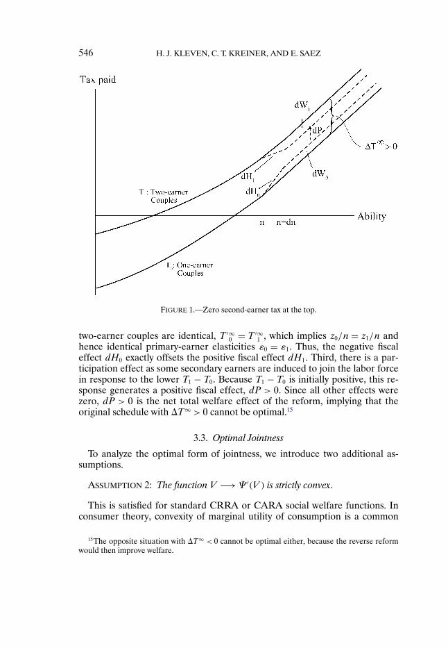
To grasp the intuition behind the zero second-earner tax at the top, considera situation where T1 − T0 does not converge to zero but instead converges toT∞ > 0 as illustrated on Figure 1. Consider then a reform that increases thetax on one-earner couples and decreases the tax on two-earner couples abovesome high n, and in such a way that the net mechanical effect on governmentrevenue is zero.14 These tax burden changes are achieved by increasing themarginal tax rate for one-earner couples in a small band (n�n+ dn) and low-ering the marginal tax rate for two-earner couples in this band.

What are the welfare effects of the reform? First, there are direct welfareeffects as the reform redistributes income from one-earner couples (who losedW0) to two-earner couples (who gain dW1). However, because g0 and g1 haveconverged to g∞, these direct welfare effects cancel out. Second, there arefiscal effects due to earnings responses of primary earners in the small bandwhere marginal tax rates have been changed (dH0 and dH1). Because T1 − T0

has converged to a constant for large n, the marginal tax rates on one- and

12In the home production model, we also have ψ/λ≤ g0 < g1 =Ψ ′(V1)/λ→ ψ/λ.13Conversely, in the case of a bounded ability distribution, the top marginal tax rate on primary

earnings would be zero, but then the tax on the secondary earner would be positive.14Because q and hence P(q|n) have converged, revenue neutrality requires that the tax changes

on one- and two-earner couples are dT0 = dT/(1 − P(q)) and dT1 = −dT/P(q), respectively.

546 H. J. KLEVEN, C. T. KREINER, AND E. SAEZ

FIGURE 1.—Zero second-earner tax at the top.

two-earner couples are identical, T ′∞0 = T ′∞

1 , which implies z0/n = z1/n andhence identical primary-earner elasticities ε0 = ε1. Thus, the negative fiscaleffect dH0 exactly offsets the positive fiscal effect dH1. Third, there is a par-ticipation effect as some secondary earners are induced to join the labor forcein response to the lower T1 − T0. Because T1 − T0 is initially positive, this re-sponse generates a positive fiscal effect, dP > 0. Since all other effects werezero, dP > 0 is the net total welfare effect of the reform, implying that theoriginal schedule with T∞ > 0 cannot be optimal.15

3.3. Optimal Jointness

To analyze the optimal form of jointness, we introduce two additional as-sumptions.

ASSUMPTION 2: The function V −→Ψ ′(V ) is strictly convex.

This is satisfied for standard CRRA or CARA social welfare functions. Inconsumer theory, convexity of marginal utility of consumption is a common

15The opposite situation with T∞ < 0 cannot be optimal either, because the reverse reformwould then improve welfare.

OPTIMAL INCOME TAXATION OF COUPLES 547

assumption, because it captures the notion of prudence and generates precau-tionary savings. As shown below, this assumption captures the central idea thatsecondary earnings matter less and less for social marginal welfare as primaryearnings increase.

ASSUMPTION 3: q and n are independently distributed.

Abstracting from correlation in spouse characteristics (assortative match-ing) allows us to isolate the implications of the spousal interaction occurringthrough the social welfare function. In Section 4, we examine numerically howassortative matching affects our results.

To establish an intuition on the optimal form of jointness, let us considera tax reform introducing a little bit of jointness around the optimal separabletax system. For the work cost model, we will argue that the optimal separableschedule can be improved by introducing a little bit of negative jointness.16

A separable schedule is one where T ′0 = T ′

1, implying that T1 − T0, q, andP(q) are constant in n. In the work cost model, we would have T1 −T0 > 0 dueto the property g0 − g1 > 0. As discussed above, this property follows from thefact that, at a given n, being a two-earner couple is a signal of low work costsand being better off than one-earner couples. Moreover, under Assumptions 2and 3, and starting from a separable tax system, g0 − g1 is decreasing in n.Intuitively, as primary-earner ability increases, the contribution of secondaryearnings to couple utility is declining in relative terms, and therefore the valueof redistribution from two- to one-earner couples is declining. Formally, underseparable taxation and Assumption 3, we have that q=w−(T1 −T0), P(q|n)=P(q), and p(q|n)= p(q) are constant in n. Then, from the definitions of g0(n)and g1(n), we obtain

d[g0(n)− g1(n)]dn

=[Ψ ′′(V0)

λ−

∫ q

0Ψ ′′(V0 + q− q)p(q)dq

λ · P(q)

]· V0 < 0�(10)

where we have used V1 = V0 + q from equation (4). Since Ψ ′′(·) is increasing(by Assumption 2) and V0 is increasing in n, it follows that the expression in(10) is negative.

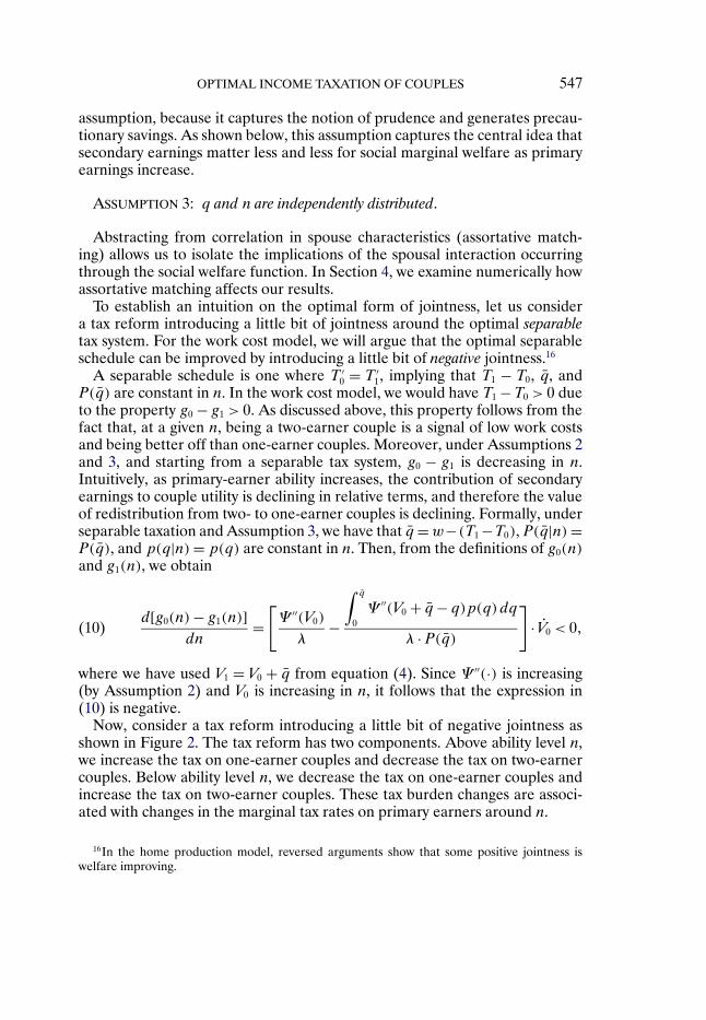
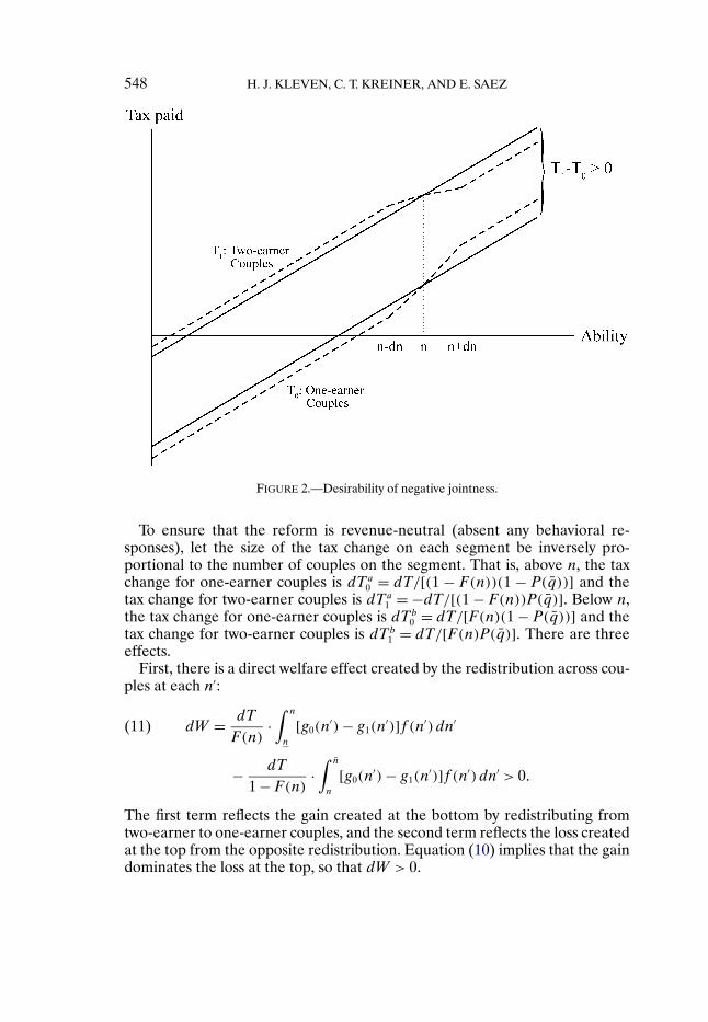
Now, consider a tax reform introducing a little bit of negative jointness asshown in Figure 2. The tax reform has two components. Above ability level n,we increase the tax on one-earner couples and decrease the tax on two-earnercouples. Below ability level n, we decrease the tax on one-earner couples andincrease the tax on two-earner couples. These tax burden changes are associ-ated with changes in the marginal tax rates on primary earners around n.

16In the home production model, reversed arguments show that some positive jointness iswelfare improving.

548 H. J. KLEVEN, C. T. KREINER, AND E. SAEZ

FIGURE 2.—Desirability of negative jointness.

To ensure that the reform is revenue-neutral (absent any behavioral re-sponses), let the size of the tax change on each segment be inversely pro-portional to the number of couples on the segment. That is, above n, the taxchange for one-earner couples is dTa0 = dT/[(1 − F(n))(1 − P(q))] and thetax change for two-earner couples is dTa1 = −dT/[(1 − F(n))P(q)]. Below n,the tax change for one-earner couples is dTb0 = dT/[F(n)(1 − P(q))] and thetax change for two-earner couples is dTb1 = dT/[F(n)P(q)]. There are threeeffects.

First, there is a direct welfare effect created by the redistribution across cou-ples at each n′:

dW = dT

F(n)·∫ n

n

[g0(n′)− g1(n

′)]f (n′)dn′(11)

− dT

1 − F(n) ·∫ n

n

[g0(n′)− g1(n

′)]f (n′)dn′ > 0�

The first term reflects the gain created at the bottom by redistributing fromtwo-earner to one-earner couples, and the second term reflects the loss createdat the top from the opposite redistribution. Equation (10) implies that the gaindominates the loss at the top, so that dW > 0.

OPTIMAL INCOME TAXATION OF COUPLES 549

Second, there are fiscal effects associated with earnings responses by pri-mary earners induced by the changes in T ′

0 and T ′1 around n. Since the reform

increases the marginal tax rate for one-earner couples around n and reduces itfor two-earner couples, the earnings responses are opposite. As we start fromseparable taxation, T ′

0 = T ′1, and hence identical primary-earner elasticities,

ε0 = ε1, the fiscal effects of primary earner responses cancel out exactly.Third, the reform creates participation responses by secondary earners.

Above n, nonworking spouses will be induced to join the labor force. Belown, working spouses have an incentive to drop out. Because spouse characteris-tics q and n are independent, and since we start from a separable tax system,the participation elasticity η= q ·p(q)/P(q) and T1 −T0 are initially constant.Therefore, the fiscal implications of these responses also cancel out exactly.

Therefore, dW > 0 is the net total welfare effect of the reform. Hence, underAssumptions 1–3, introducing a little bit of negative jointness increases welfare.This perturbation argument suggests that, for the work cost model, the opti-mal incentive scheme will be associated with negative jointness, a point we willprove formally after introducing a final technical assumption:

ASSUMPTION 4: The function x−→ x ·p(w−x)/[P(w−x) · (1−P(w−x))]is increasing and p(q)/P(q)≤ P(q)/ ∫ q

0 P(q′)dq′ for all q.

This assumption is satisfied for isoelastic work cost distributions, P(q) =(q/qmax)

η, where the participation elasticity of secondary earners is constantand equal to η.17

PROPOSITION 3: Under Assumptions 1–4 and if the optimal solution is notassociated with bunching, the tax system is characterized by the following models:

Work Cost Model: 1a. Positive tax on secondary-earner income, τ > 0 for alln ∈ [n� n]. 1b. Negative jointness, T ′

1 ≤ T ′0 and τ ≤ 0 for all n ∈ [n� n].

Home Production Model: 2a. Negative tax on secondary-earner income, τ < 0for all n ∈ [n� n]. 2b. Positive jointness, T ′

1 ≥ T ′0 and τ ≥ 0 for all n ∈ [n� n].

PROOF: We consider the work cost model.18 Suppose by contradiction thatT ′

1 > T′0 for some n. Then, because T ′

0 and T ′1 are continuous in n and because

T ′1 = T ′

0 at the top and bottom skills, there exists an interval (na�nb) whereT ′

1 > T′0 and where T ′

1 = T ′0 at the end points na and nb. This implies that z1 < z0

17Assumption 4 can be seen as a counterpart to Assumption 1 for the participation margin. Itensures that the participation response does not decrease too fast with the tax rate. It was notneeded for the small reform argument, because in that case the efficiency effects from participa-tion responses cancel out to the first order.

18Results 2a and 2b may be established by reversing all inequalities in the proof below.

550 H. J. KLEVEN, C. T. KREINER, AND E. SAEZ

on (na�nb) with equality at the end points. Assumption 1 implies

ε1T′1/(1 − T ′

1)=(

1 − h′(z1

n

))/((z0

n

)h′′

(z1

n

))

>

(1 − h′

(z0

n

))/((z1

n

)h′′

(z0

n

))

= ε0T′0/(1 − T ′

0)

on (na�nb). Then, because of our no bunching assumption, (7) and (8) imply

Ω0(n)≡ 11 − P

∫ n

n

[(1 − g0)(1 − P)+T ·p]f (n′)dn′

<1P

∫ n

n

[(1 − g1)P −T ·p]f (n′)dn′ ≡Ω1(n)

on (na�nb) with equality at the end points. This implies that the derivatives ofthe above expressions with respect to n, at the end points, obey the inequalitiesΩ0(na) ≤ Ω1(na) and Ω0(nb) ≥ Ω1(nb). At the end points, we have T ′

1 = T ′0,

z0 = z1, and V0 = V1, which implies ˙q= 0 and P = 0. Hence, the inequalities inderivatives can be written as

1 − g0 +T ·p/(1 − P){≥ 1 − g1 −T ·p/P at na,

≤ 1 − g1 −T ·p/P at nb.

Combining these inequalities, we obtain

T ·pP(1 − P)

∣∣∣∣na

≥ g0(na)− g1(na) > g0(nb)− g1(nb)≥ T ·pP(1 − P)

∣∣∣∣nb

�

From our small reform argument, the middle inequality is intuitive and weprove it formally in Appendix B. Using that q = w − T at na and nb, alongwith the first part of Assumption 4, we obtain T(na) > T(nb). However,given T ′

1 > T′0 and hence z1 < z0, we have ˙q < 0 on the interval (na�nb). This

implies q(na)≥ q(nb) and thus T(na)≤ T(nb). This generates a contradic-tion, which proves that T ′

1 ≤ T ′0 for all n.

Property 1a follows easily from 1b. Since we now have T ′1 ≤ T ′

0 on (n� n) withequality at the end points, we obtain Ω0(n) ≥ Ω1(n) on (n� n) with equalityat the end points. Then we have that Ω0(n) ≤ Ω1(n), which implies 1 − g0 +T · p/(1 − P)≥ 1 − g1 − T · p/P at n. Because g0(n)− g1(n) > 0, we haveT(n) > 0. Finally, T ′

1 ≤ T ′0 and hence z1 ≥ z0 implies ˙q = V1 − V0 ≥ 0 from

equation (3). Hence, τ(n) = (w − q(n))/w ≥ (w − q(n))/w = T(n)/w > 0for all n, where the last equality follows from T ′

1 = T ′0 = 0 at n. Q.E.D.

OPTIMAL INCOME TAXATION OF COUPLES 551

We may summarize our findings as follows. In the work cost model, second-earner participation is a signal of low work costs and hence being better offthan one-earner couples. This implies g0(n) > g1(n), which makes it optimalto tax secondary earnings, τ > 0. In the home production model, second-earnerparticipation is a signal of low ability in home production and hence beingworse off than one-earner couples. In this model, it is therefore optimal tosubsidize secondary earnings, τ < 0.19

In either model, the redistribution between one- and two-earner couples givesrise to a distortion in the entry–exit decision of secondary earners, creatingan equity–efficiency trade-off. The size of the efficiency cost does not dependon the ability of the primary earner, because spousal characteristics q and nare independently distributed. An increase in n therefore influences the op-timal second-earner distortion only through its impact on the equity gain asreflected by g0(n)− g1(n). Because the contribution of the secondary earnerto couple utility is declining in relative terms, the value of redistribution be-tween one- and two-earner couples is declining in n, that is, g0(n) − g1(n)is decreasing in n. Therefore, the second-earner distortion is declining withprimary earnings. As shown in Proposition 2, if the ability distribution of pri-mary earners is unbounded, the secondary-earner distortion tends to zero atthe top.20

Instead of working with a social welfare function Ψ(·), if we assume exoge-nous Pareto weights (λ0(n)�λ1(n)), then the social marginal welfare weightsg0(n) = λ0(n)/λ and g1 = λ1(n)/λ would be fixed a priori. Optimal tax for-mulas (7) and (8) would carry over. Positive versus negative second-earner taxrates would depend on the sign of λ0(n) − λ1(n), and positive versus nega-tive jointness would depend on the profile of λ0(n)− λ1(n) with respect to n.The asymptotic zero tax result would be true iff λ0(n)− λ1(n)→ 0 as n→ ∞.Hence, all results would depend on the assumptions made on the exogenousPareto weights.

Unlike our reform argument, the negative jointness result in Proposition 3relies on an assumption of no bunching. As we discuss in the online supplemen-tal material, when redistributive tastes are weak, the optimal solution is closeto the no-tax situation and therefore should display no bunching.21 For strongredistributive tastes, our numerical simulations show that there is no bunchingin a wide set of cases.

19In a more general model with both costs of work and home production, there should be a tax(subsidy) on secondary earnings if there is more (less) heterogeneity in work costs than in homeproduction abilities (see the online supplemental material for a discussion).

20If Ψ is quadratic, then g0 − g1 is constant in n and the optimal tax system is separable. If Ψ ′

is concave, then g0 − g1 increases in n and the distortion on spouses actually increases with n.As discussed above, the case Ψ ′ convex (Assumption 2) fits best with the intuition that secondaryearnings affect marginal social utility less when primary earnings are higher.

21This is also true in the one-dimensional model. We provide a simple formal proof of this inthe online supplemental material.

552 H. J. KLEVEN, C. T. KREINER, AND E. SAEZ

4. NUMERICAL CALIBRATION FOR THE UNITED KINGDOM

Numerical simulations are conceptually important (i) to assess whether ourno bunching assumption in Proposition 3 is reasonable, (ii) to assess howquickly the second-earner tax rate decreases to zero (scope of Proposition 2),and (iii) to analyze if and to what extent optimal schedules resemble real-worldschedules.

We focus on the more realistic and traditional work cost model and make thefollowing parametric assumptions: (a) h(x)= ε/(1 + ε)x1+1/ε so that the elas-ticity of primary earnings ε is constant; (b) q is distributed as a power functionon the interval [0� qmax] with distribution function P(q) = (q/qmax)

η, implyinga constant second-earner participation elasticity η; (c) the social welfare func-tion is CRRA, Ψ(V ) = V 1−γ/(1 − γ), where γ > 0 measures preferences forequity.

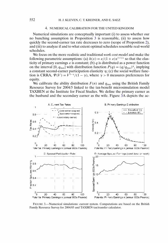
We calibrate the ability distribution F(n) and qmax using the British FamilyResource Survey for 2004/5 linked to the tax-benefit microsimulation modelTAXBEN at the Institute for Fiscal Studies. We define the primary earner asthe husband and the secondary earner as the wife. Figure 3A depicts the ac-

FIGURE 3.—Numerical simulations: current system. Computations are based on the BritishFamily Resource Survey for 2004/05 and TAXBEN tax/transfer calculator.

OPTIMAL INCOME TAXATION OF COUPLES 553

tual tax rates T ′0, T ′

1, and τ faced by couples in the United Kingdom. As inSaez (2001), f (n) is calibrated such that, at the actual marginal tax rates, theresulting distribution of primary earnings matches the empirical earnings dis-tribution for married men. The top quintile of the distribution (n≥ £46�000) isapproximated by a Pareto distribution with coefficient a= 2, a good approxi-mation according to Brewer, Saez, and Shephard (2008). Figure 3B depicts thecalibrated density distribution f (n). The dashed line is the raw density distrib-ution and the solid line is the smoothed density that we use to obtain smoothoptimal schedules.

Figure 3C shows that the participation rate of wives conditional on husbands’earnings is fairly constant across the earnings distribution and equal to 75% onaverage. Figure 3D shows that average female earnings, conditional on partic-ipation, are slightly increasing in husbands’ earnings. Our model with homoge-nous secondary earnings does not capture this feature. We therefore assume(except when we explore the effects of assortative matching below) that qmax

(and hence q) is independent of n. We calibrate qmax so that the average par-ticipation rate (under the current tax system) matches the empirical rate. Thew parameter is set equal to average female earnings conditional on participa-tion.22

Based on the empirical labor supply literature for the United Kingdom(see Brewer, Saez, and Shephard (2008)), we assume ε = 0�25 and η = 0�5in our benchmark case. Based on estimates of the curvature of utility func-tions consistent with labor supply responses, we set γ equal to 1 (see, e.g.,Chetty (2006)). Finally, we assume that the simulated optimal tax system(net of transfers) must collect as much tax revenue (net of transfers) as theactual U.K. tax system, which we compute using TAXBEN and the empir-ical data. In all simulations, we check that the implementation conditions(zl(n) increasing in n) are satisfied so that there is no bunching. All techni-cal details of the simulations are described in the online supplemental mater-ial.

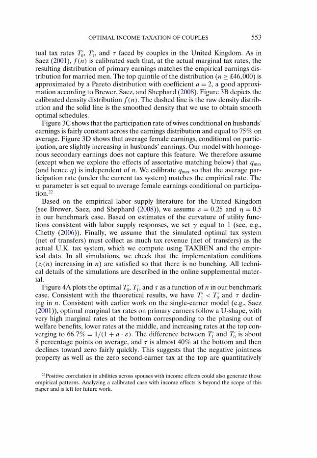
Figure 4A plots the optimal T ′0, T ′

1, and τ as a function of n in our benchmarkcase. Consistent with the theoretical results, we have T ′

1 < T′0 and τ declin-

ing in n. Consistent with earlier work on the single-earner model (e.g., Saez(2001)), optimal marginal tax rates on primary earners follow a U-shape, withvery high marginal rates at the bottom corresponding to the phasing out ofwelfare benefits, lower rates at the middle, and increasing rates at the top con-verging to 66�7% = 1/(1 + a · ε). The difference between T ′

1 and T ′0 is about

8 percentage points on average, and τ is almost 40% at the bottom and thendeclines toward zero fairly quickly. This suggests that the negative jointnessproperty as well as the zero second-earner tax at the top are quantitatively

22Positive correlation in abilities across spouses with income effects could also generate thoseempirical patterns. Analyzing a calibrated case with income effects is beyond the scope of thispaper and is left for future work.

554 H. J. KLEVEN, C. T. KREINER, AND E. SAEZ

FIGURE 4.—Optimal tax simulations. Computations are based on the British Family ResourceSurvey for 2004/05 and TAXBEN tax/transfer calculator.

significant results and not just theoretical curiosities. Finally, notice that taxrates on primary earners are substantially higher than on secondary earnersbecause the primary-earner elasticity is smaller than the secondary-earner elas-ticity.

Figure 4B introduces a positive correlation in spousal abilities by lettingqmax depend on n, so that the fraction of working spouses (under the cur-rent tax system) increases smoothly from 55% to 80% across the distri-bution of n. This captures indirectly the positive correlation in earningsshown in Figure 3D. Figure 4B shows that introducing this amount of cor-relation has minimal effects on optimal tax rates. Compared to no corre-lation, the second-earner tax is slightly higher at the bottom, which rein-forces the declining profile for τ. Figure 4C explores the effects of increas-ing redistributive tastes γ from 1 to 2. Not surprisingly, this increases taxrates across the board. Figure 4D considers a higher primary-earner elastic-ity (ε= 0�5). As expected, this reduces primary-earner tax rates (especially atthe top).

OPTIMAL INCOME TAXATION OF COUPLES 555

Importantly, none of our simulations displays bunching, which suggests thatthere is no bunching in a wide set of cases and hence that Proposition 3 appliesbroadly.

Comparing the simulations with the empirical tax rates in Figure 3A is il-luminating. The actual tax-transfer system also features negative jointness,with the second-earner tax rate falling from about 40% at the bottom toabout 20% at the middle and upper parts of the primary earnings distrib-ution. This may seem surprising at first glance given that the United King-dom operates an individual income tax. However, income transfers in theUnited Kingdom (as in virtually all Organization for Economic Coopera-tion and Development countries) are means tested based on family income.The combination of an individual income tax and a family-based, means-tested welfare system generates negative jointness: a wife married to a low-income husband will be in the phase-out range of welfare programs and hencefaces a high tax rate, whereas a wife married to a high-income husband isbeyond benefit phase-out and hence faces a low tax rate because the in-come tax is individual. Thus, our theoretical and numerical findings of neg-ative jointness may provide a justification for the current practice in manycountries of combining family-based transfers with individual income taxa-tion.23�24

Clearly, our calibration abstracts from several potentially important aspectssuch as income effects, heterogeneity in secondary earnings, and endogenousmarriage. Hence, our simulations should be seen as an illustration of our the-ory rather than actual policy recommendation. More complex and comprehen-sive numerical calibrations are left for future work.

APPENDIX A: PROOF OF PROPOSITION 1

The government maximizes

W =∫ n

n

{∫ q

0Ψ(V1 − qw)p(q|n)dq

+∫ ∞

q

Ψ (V0 + qh)p(q|n)dq}f (n)dn�

23Indeed, Immervoll, Kleven, Kreiner, and Verdelin (2008) showed that most European Unioncountries feature negative jointness at the bottom driven by family-based transfers.

24As for the size and profile of primary-earner tax rates, the current U.K. schedule displayslower rates at the very bottom (below £6–7K) than the simulations. This might be justified byparticipation responses for low-income primary earners (Saez (2002)), not incorporated in ourmodel. Above £6–7K, the current U.K. tax system does display a weak U-shape with the highestmarginal rates at the bottom and modest increases above £40K.

556 H. J. KLEVEN, C. T. KREINER, AND E. SAEZ

where q = V1 − V0, q = qw + qh and either qw = 0 or qh = 0. The objective ismaximized subject to the budget constraint∫ n

n

{[z1 +w− nh

(z1

n

)− V1

]P(q|n)

+[z0 − nh

(z0

n

)− V0

](1 − P(q|n))

}f (n)dn≥ 0

and the constraints from household optimization, Vl = −h(zl/n)+zl/nh′(zl/n)for l = 0�1. Let λ, μ0(n), and μ1(n) be the associated multipliers, and letH(z0� z1� V0� V1�μ0�μ1�λ�n) be the Hamiltonian.

We demonstrate the existence of a measurable solution n→ z(n) in the on-line supplemental material. The Pontryagin maximum principle then providesnecessary conditions that hold at the optimum:

(i) There exist absolutely continuous multipliers (μ0(n)�μ1(n)) such thaton (n� n), μl(n)= −∂H/∂Vl almost everywhere in n with transversality condi-tions μl(n)= μl(n)= 0 for l= 0�1.

(ii) We have H(z(n)�V (n)�μ(n)�λ�n) ≥ H(z�V (n)�μ(n)�λ�n) for all zalmost everywhere in n. The first-order conditions associated with this maxi-mization condition are

∂H

∂z0= μ0

n· z0

n· h′′

(z0

n

)+ λ ·

(1 − h′

(z0

n

))· (1 − P(q|n)) · f (n)(A1)

= 0�

∂H

∂z1= μ1

n· z1

n· h′′

(z1

n

)+ λ ·

(1 − h′

(z1

n

))· P(q|n) · f (n)= 0�(A2)

By Assumption 1, ϕ(x) ≡ (1 − h′(x))/(xh′′(x)) is decreasing in x. Rewriting(A1) as ϕ(z0/n) = −μ0(n)/[λ(1 − P(q|n))nf (n)], Assumption 1 implies that(A1) has a unique solution z0(n), and that ∂H/∂z0 > 0 for z0 < z0(n) and∂H/∂z0 < 0 for z0 > z0(n). This ensures that z0(n) is indeed the global max-imum for H as required in the Pontryagin maximum principle. Obviously, thestate variable V (n) is continuous in n. Thus, ϕ(z0(n)/n) = −μ0(n)/[λ(1 −P(V1(n) − V0(n)|n))nf (n)] implies that z0(n) is continuous in n.25 Similarly,z1(n) is continuous in n.26 By defining T ′

l ≡ 1 − h′(zl(n)/n), we have that(T ′

0�T′1) is also continuous in n.27

25The assumption that n→ f (n) and x→ h′′(x) are continuous is required here.26Those continuity results also apply to the one-dimensional case and were explicitly derived

by Mirrlees (1971) under a condition equivalent to our Assumption 1. The subsequent literaturealmost always assumes continuity.

27Notice that we adopt this definition of T ′l everywhere, including points where z→ T(z) has

a kink.

OPTIMAL INCOME TAXATION OF COUPLES 557

The conditions μl(n)= −∂H/∂Vl for l= 0�1 imply

−μ0(n)=∫ ∞

q

Ψ ′(V0 + qh)p(q|n)f (n)dq− λ(1 − P(q|n))f (n)(A3)

− λ[T1 − T0]p(q|n)f (n)�−μ1(n)=

∫ q

0Ψ ′(V1 − qw)p(q|n)f (n)dq− λP(q|n)f (n)T1(A4)

+ λ[−T0]p(q|n)f (n)�Using the definition of welfare weights, g0(n) and g1(n), we integrate (A3) and(A4) using the upper transversality conditions so as to obtain

−μ0(n)

λ=

∫ n

n

{[1 − g0(n′)](1 − P(q|n′))f (n′)

+ [T1 − T0]p(q|n′)f (n′)}dn′�

−μ1(n)

λ=

∫ n

n

{[1 − g1(n′)]P(q|n′)f (n′)− [T1 − T0]p(q|n′)f (n′)

}dn′�

Inserting these two equations into (A1) and (A2), noting that T ′l = 1 − h′

l, andusing the elasticity definition εl = h′(zl/n)/[zl/nh′′(zl/n)], we obtain equa-tions (7) and (8) in Proposition 1.

The transversality conditions μ0 = μ1 = 0 at n and n combined with (A1)and (A2) imply that h′(z0/n)= h′(z1/n)= 1 and hence T ′

1 = T ′0 = 0 at n and n.

As shown in the online supplemental material, a necessary and sufficientcondition for implementability is that z0 and z1 are weakly increasing in n (ex-actly as in the one-dimensional Mirrlees model). If (7) and (8) generate de-creasing ranges for z0 or z1, there is bunching and the formulas do not apply onthe bunching portions. It is straightforward to include the constraints zl(n)≥ 0in the maximization problem (as in Mirrlees (1986)).28 On a bunching portion,zl(n) is constant (say equal to z∗) and hence T ′

l = 1 −h′(z∗/n) remains contin-uous in n as stated in Proposition 1, but z→ T ′

l (z) jumps discontinuously at z∗

and z → Tl(z) displays a kink at z∗. Hence the optimal solution z → T(z) iscontinuous and z→ T ′(z) is piecewise continuous.

We do not establish that the solution is unique, but uniqueness is notrequired for our results. Uniqueness would follow from the concavity of(z�V )→H(z�V �μ(n)�λ�n), but this is a very strong assumption. In the simu-lations, we can check numerically that, under our parametric assumptions, thestronger concavity assumptions required for uniqueness hold in the domain ofinterest so that we are sure the numerical solution we find is indeed the globaloptimum.

28We do not include such constraints formally so as to simplify the exposition and because ourmain Proposition 3 assumes no bunching and our simulations never involve bunching.

558 H. J. KLEVEN, C. T. KREINER, AND E. SAEZ

APPENDIX B: PROOF OF LEMMA IN PROPOSITION 3

LEMMA B1: Under Assumptions 1–4, if T ′1 > T

′0 on (na�nb) with equality at the

end points, then g0(na)− g1(na) > g0(nb)− g1(nb).

PROOF: We have q= V1 −V0 and g0 −g1 =Ψ ′(V0)/λ−∫ q

0 Ψ′(V1 −q)p(q)dq/

(λ ·P(q)) > 0 (inequality follows from Ψ ′ decreasing). Differentiating with re-spect to n, we obtain

g0 − g1 = V0 · Ψ′′(V0)

λ− V1 ·

∫ q

0Ψ ′′(V1 − q)p(q)dq

λ · P(q)

+ p(q) ˙qP(q)

·[∫ q

0Ψ ′(V1 − q)p(q)dq

λ · P(q) − Ψ ′(V0)

λ

]�

which can be rewritten as

g0 − g1 = V1 ·[Ψ ′′(V0)

λ−

∫ q

0Ψ ′′(V0 + q− q)p(q)dq

λ · P(q)

](B1)

+ ˙q ·[−(g0 − g1) · p(q)

P(q)− Ψ ′′(V0)

λ

]�

The first term in (B1) is negative, because V1 > 0 and Ψ ′′ is increasing (byAssumption 2) so that the term inside the first square brackets is negative. On(na�nb), z1 < z0 and hence ˙q < 0. Moreover, convexity of Ψ ′ implies Ψ ′(V0)−Ψ ′(V0 + q− q)≤ −Ψ ′′(V0) · (q− q) and hence

g0 − g1 =

∫ q

0[Ψ ′(V0)−Ψ ′(V0 + q− q)]p(q)dq

λ · P(q)(B2)

≤ −Ψ ′′(V0) ·

∫ q

0P(q)dq

λ · P(q) �

where we have used that∫ q

0 (q−q)p(q)dq= ∫ q

0 P(q)dq by integration by partsand P(0)= 0. Combining (B2) and the second part of Assumption 4, we have(g0 − g1) ·p(q)/P(q)≤ −Ψ ′′(V0)/λ� Thus, the second term in square bracketsin (B1) is nonnegative, making the entire second term in (B1) nonpositive. Asa result, g0(n)− g1(n) < 0 on (na�nb) and the lemma is proven. Q.E.D.

OPTIMAL INCOME TAXATION OF COUPLES 559

REFERENCES

ARMSTRONG, M. (1996): “Multiproduct Nonlinear Pricing,” Econometrica, 64, 51–75. [538]BOSKIN, M., AND E. SHESHINSKI (1983): “Optimal Tax Treatment of the Family: Married Cou-

ples,” Journal of Public Economics, 20, 281–297. [538]BRETT, C. (2006): “Optimal Nonlinear Taxes for Families,” International Tax and Public Finance,

14, 225–261. [538]BREWER, M., E. SAEZ, AND A. SHEPHARD (2008): “Means Testing and Tax Rates on Earnings,”

IFS Working Paper. Forthcoming in Reforming the Tax System for the 21st Century, Oxford Uni-versity Press, 2009. [553]

CHETTY, R. (2006): “A New Method of Estimating Risk Aversion,” American Economic Review,96, 1821–1834. [553]

CREMER, H., J. LOZACHMEUR, AND P. PESTIEAU (2007): “Income Taxation of Couples and theTax Unit Choice,” CORE Discussion Paper No. 2007/13. [538]

CREMER, H., P. PESTIEAU, AND J. ROCHET (2001): “Direct versus Indirect Taxation: The Designof the Tax Structure Revisited,” International Economic Review, 42, 781–799. [538]

IMMERVOLL, H., H. J. KLEVEN, C. T. KREINER, AND N. VERDELIN (2008): “An Evaluation of theTax-Transfer Treatment of Married Couples in European Countries,” Working Paper 2008-03,EPRU. [555]

KLEVEN, H. J., C. T. KREINER, AND E. SAEZ (2006): “The Optimal Income Taxation of Couples,”Working Paper 12685, NBER. [538,544]

(2009): “Supplement to ‘The Optimal Income Taxation of Couples’,” Econometrica Sup-plementary Material, 77, http://www.econometricsociety.org/ecta/Supmat/7343_Proofs.pdf andhttp://www.econometricsociety.org/ecta/Supmat/7343_Data and programs.zip. [539]

MIRRLEES, J. A. (1971): “An Exploration in the Theory of Optimal Income Taxation,” Review ofEconomic Studies, 38, 175–208. [537,543,556]

(1976): “Optimal Tax Theory: A Synthesis,” Journal of Public Economics, 6, 327–358.[538]

(1986): “The Theory of Optimal Taxation,” in Handbook of Mathematical Economics,Vol. 3, ed. by K. J. Arrow and M. D. Intrilligator. Amsterdam: Elsevier. [538,557]

RAMEY, V. A. (2008): “Time Spent in Home Production in the 20th Century: New EstimatesFrom Old Data,” Working Paper 13985, NBER. [540]

ROCHET, J., AND C. PHILIPPE (1998): “Ironing, Sweeping, and Multi-Dimensional Screening,”Econometrica, 66, 783–826. [538]

SAEZ, E. (2001): “Using Elasticities to Derive Optimal Income Tax Rates,” Review of EconomicStudies, 68, 205–229. [540,544,545,553]

(2002): “Optimal Income Transfer Programs: Intensive versus Extensive Labor SupplyResponses,” Quarterly Journal of Economics, 117, 1039–1073. [555]

SCHROYEN, F. (2003): “Redistributive Taxation and the Household: The Case of Individual Fil-ings,” Journal of Public Economics, 87, 2527–2547. [538]

Dept. of Economics, London School of Economics, Houghton Street, LondonWC2A 2AE, U.K. and Economic Policy Research Unit, Dept. of Economics, Uni-versity of Copenhagen, Copenhagen, Denmark and Centre for Economic PolicyResearch, London, U.K.; h.j.kleven@lse.ac.uk,

Dept. of Economics, University of Copenhagen, Studiestraede 6, # 1455 Copen-hagen, Denmark and Economic Policy Research Unit, Dept. of Economics, Uni-versity of Copenhagen, Copenhagen, Denmark and CESifo, Munich, Germany,

and

560 H. J. KLEVEN, C. T. KREINER, AND E. SAEZ

Dept. of Economics, University of California–Berkeley, 549 Evans Hall 3880,Berkeley, CA 94720, U.S.A. and NBER; saez@econ.berkeley.edu.

Manuscript received August, 2007; final revision received August, 2008.

Econometrica Supplementary Material

SUPPLEMENT TO “THE OPTIMAL INCOME TAXATIONOF COUPLES”

(Econometrica, Vol. 77, No. 2, March, 2009, 537–560)

BY HENRIK JACOBSEN KLEVEN, CLAUS THUSTRUP KREINER,AND EMMANUEL SAEZ

Section S1 shows that a given path of earnings (z0(n)� z1(n)) is implementable. Sec-tion S2 provides conditions for the existence of a solution to the maximization problem.Section S3 discusses conditions ensuring no bunching in the optimum. Section S4 dis-cusses the outcome of a more general model with heterogeneity in both work costs andhome production abilities. Section S5 provides technical details of the simulations.

S1. IMPLEMENTATION

AS IN THE ONE-DIMENSIONAL MECHANISM DESIGN theory, we define imple-mentability as follows: An action profile (z0(n)� z1(n))n∈(n� n) is implementableif and only if there exist transfer functions (c0(n)� c1(n))n∈(n� n) such that(zl(n)� cl(n))l∈{0�1}�n∈(n� n) is a simple truthful mechanism.1 The central imple-mentability theorem of the one-dimensional case carries over to our model.

LEMMA S.1: An action profile (z0(n)� z1(n))n∈(n� n) is implementable if and onlyif z0(n) and z1(n) are both nondecreasing in n.

PROOF: The utility function c − nh(z/n) satisfies the classic single crossing(Spence–Mirrlees) condition (here equal to x ·h′′(x) > 0 for all x > 0). Hence,from the one-dimensional case, we know that z(n) is implementable, that is,there is some c(n) such that c(n) − nh(z(n)/n) ≥ c(n′) − nh(z(n′)/n) for alln�n′ if and only if z(n) is nondecreasing.2

Suppose (z0(n)� z1(n)) is implementable, implying that there exists (c0(n)�c1(n)) such that (zl(n)� cl(n))l∈{0�1}�n∈(n� n) is a simple truthful mechanism. Thatimplies in particular that cl(n) − nh(zl(n)/n) ≥ cl(n

′) − nh(zl(n′)/n) for all

n�n′ and for l = 0�1. Hence, the one-dimensional result implies that z0(n) andz1(n) are nondecreasing.

Conversely, suppose that z0(n) and z1(n) are nondecreasing. Because z0(n)is nondecreasing, the one-dimensional result implies there is c0(n) such that

1A mechanism is defined as truthful if there is a q(n) so that (i) when q < q(n), the set (l′ =1�n′ = n) maximizes u(zl′(n

′)� l′� cl′(n′)� (n�q)) over all (l′�n′); (ii) when q ≥ q(n), the set (l′ =0�n′ = n) maximizes u(zl′(n′)� l′� cl′(n′)� (n�q)) over all (l′�n′).

2As an informal reminder, recall that if z(n) is implementable, then the first-order con-dition is c(n) − h′(z(n)/n)z(n) = 0 and the second-order condition is c − zh′(z(n)/n) −(z2/n)h′′(z(n)/n) ≤ 0. Differentiating the first-order condition leads to c − zh′(z(n)/n) −(z2/n)h′′(z(n)/n) + (z(n)/n)h′′(z(n)/n)(z/n) = 0. Combining with the second-order conditionimplies (z(n)/n)h′′(z(n)/n)z ≥ 0, which implies z ≥ 0 using the Spence–Mirrlees condition.

© 2009 The Econometric Society DOI: 10.3982/ECTA7343

2 H. J. KLEVEN, C. T. KREINER, AND E. SAEZ

c0(n)−nh(z0(n)/n)≥ c0(n′)−nh(z0(n

′)/n). Similarly, there is c1(n) such thatc1(n)− nh(z1(n)/n)≥ c1(n

′)− nh(z1(n′)/n).

It is easy to show that the mechanism (zl(n)� cl(n))l∈{0�1}�n∈(n� n) is actuallytruthful. Define Vl(n) = cl(n) − nh(zl(n)/n) for l = 0�1 and q(n) = V1(n) −V0(n). We only need to prove the cross-inequalities. For all n�n′� q ≥ q(n),

u(z0(n)�0� c0(n)� (n�q))

= V0(n)≥ V1(n)− q ≥ u(z1(n′)�1� c1(n

′)� (n�q));for all n�n′� q < q(n),

u(z1(n)�1� c1(n)� (n�q))

= V1(n)− q ≥ V0(n)≥ u(z0(n′)�0� c0(n

′)� (n�q))�

The key assumption that allows us to obtain those simple results is the fact thatq is separable in our utility specification. Q.E.D.

S2. EXISTENCE OF A SOLUTION TO THE MAXIMIZATION PROBLEM

Formally, our maximization problem is the optimal control problemV = b(n�V � z) with maximization objective B0 = ∫ n

nb0(n�V (n))dn and con-

straint∫ n

nb1(n� z(n)�V (n))dn≥ 0, where

b(n�V � z)=(

−h

(z0

n

)+

(z0

n

)h′

(z0

n

)�−h

(z1

n

)+

(z1

n

)h′

(z1

n

))�

b0(n�V ) =[∫ V1−V0

0Ψ(V1 − qw)p(q|n)dq

+∫ ∞

V1−V0

Ψ(V0 + qh)p(q|n)dq]f (n)�

b1(n�V � z) ={[

z1 +w − nh

(z1

n

)− V1

]P(V1 − V0|n)

+[z0 − nh

(z1

n

)− V0

](1 − P(V1 − V0|n))

}f (n)�

The functions b, b0, and b1 are continuous in n and class C1 in (V � z) by as-sumption. Some convexity assumptions are required to demonstrate the exis-tence of a solution (V � z). Strict concavity of the functions b0 and b1, and strictconvexity of b in (V � z) are sufficient to obtain existence (and uniqueness); see,for example, Mangasarian (1966, Theorem 1, p. 141). However, in our appli-cation, concavity of b0 and b1 would be an unduly strong assumption.

OPTIMAL INCOME TAXATION OF COUPLES 3

It is possible to obtain existence without such strong assumptions using ourAssumption 1 and the regularity assumptions on functions f�Ψ�P , and h. Moreprecisely, according to Macki (1982, Theorem 3, p. 96), if we assume (i) an apriori bound on the path of admissible z,3 (ii) b�b0, and b1 are continuous,and (iii) the sets B(n�V �λ) = {(y�b(n�V � z))|z0 ≥ 0� z1 ≥ 0� y ≥ −b0(n�V ) −λ · b1(n�V � z)} are convex for all n�V and λ ≥ 0, then there exists an optimalcontrol z measurable on (n� n).4

Assumption (iii) is the only one that requires checking. In our problem, wehave:

B(n�V �λ)={(

y�−h

(z0

n

)+

(z0

n

)h′

(z0

n

)�

−h

(z1

n

)+

(z1

n

)h′

(z1

n

))∣∣∣z0 ≥ 0� z1 ≥ 0�

y ≥ −b0(n�V )

− λf(n) ·[(1 − P) ·

(z0 − nh

(z0

n

)− V0

)

+ P ·(w + z1 − nh

(z0

n

)− V1

)]}�

Let us denote by K(·) the inverse of the strictly increasing function x →−h(x)+ xh′(x). Note that K(0)= 0. Hence, we have

B(n�V �λ)

= {(y�x0�x1)|x0 ≥ 0�x1 ≥ 0�

y + b0(n�V ) ≥ nf (n)λ[(1 − P) · (h(K(x0))−K(x0)+ V0

)+ P · (h(K(x1))−K(x1)−w + V1

)]}�

Therefore, B(n�V �λ) is convex if x → h(K(x)) − K(x) ≡ φ(x) is convex. Bydefinition of K(x), we have −h(K(x)) + K(x)h′(K(x)) = x, hence K(x) ·h′′((K(x)) · K′(x)) = 1. Therefore, we have φ′(x) = (h′(K(x)) − 1)K′(x) =−(1−h′(K(x)))/[K(x)h′′(K(x))]. As x →K(x) is strictly increasing, Assump-tion 1 implies that φ′(x) is increasing.

3That means that we know a priori that there is some Z > 0 possibly large such that0 ≤ zl(n) ≤ Z for all n ∈ (n� n) and l = 0�1. This assumption is weak when n < ∞ as we do not ex-pect the optimal tax system to generate infinitely large subsidies that drive up earnings z withoutbound.

4Macki (1982) presented optimal control as a minimization problem. Our maximization prob-lem can be seen as minimizing − ∫

b0 dn. Macki (1982) did not include constraints such as∫b1 dn ≥ 0, but such a constraint can be added by using a standard Lagrange multiplier λ and

considering the objective b0 + λ · b1.

4 H. J. KLEVEN, C. T. KREINER, AND E. SAEZ

S3. NO BUNCHING WITH LOW REDISTRIBUTIVE TASTES

As discussed in the main text, when redistributive tastes are low, the optimalsolution is close to the laissez-faire no tax solution (where z0 = z1 = n), and,therefore, will have the property that zl is strictly increasing in n and hencedisplay no bunching.

A formal proof of this statement requires using advanced functional analysis(see Kleven, Kreiner, and Saez (2007)), but the argument is easy to understand.Let us parametrize redistributive tastes with γ and assume that social welfare isCRRA so that Ψ(V ) = V 1−γ/(1−γ). The no redistributive case is γ = 0. Whenγ = 0, the unique solution is z0 = z1 = n.5 Let us denote by zγ the solutionfor γ ≥ 0 and assume that the strong convexity assumptions hold so that thesolution is unique for γ > 0. It is possible to show that the solution is smooth inγ and can be written as zγ = z0 +γ ·Z+o(γ), where n →Z(n) is the first-orderdeviation from z0 for small γ and o(γ) is small relative to γ (in a C1 sense).Z actually satisfies a linear second-order differential equation with a uniquesmooth solution. As a result, zγ

l (n) = 1 + γ · Zl(n) + o(γ) > 0 for γ small sothat zγ does not display bunching.

This result is of course true as well in the one-dimensional case and canbe demonstrated without using advanced functional analysis. To our knowl-edge, this result has not been presented in the literature before6 and is formallyproven below.

PROPOSITION S.1: Consider the one-dimensional Mirrlees (1971) optimal in-come tax problem with Ψ(V ) = V 1−γ/(1 − γ). Assume that Assumption 1 in themain text is satisfied, n → f (n) is of class C1 and bounded away from 0, x → h(x)is of class C3, n > 0, and n < ∞. Then the solution does not display bunching forγ > 0 small enough.

PROOF: In the one-dimensional case, under the assumptions of the proposi-tion, the Hamiltonian is strictly concave in (z�V ) for γ > 0 so that the solutionis unique and given by the maximum principle first-order condition:

ϕ

(z

n

)· nf(n)=

∫ n

n

(1 − V (m)−γ

λ

)f (m)dm(S.1)

with ϕ(x) = (1 − h′(x))/(xh′′(x)), λ = ∫ n

nV (n)−γf (n)dn, and V (n) =

−h′(z/n) + (z/n)h′(z/n) ≥ 0. Transversality conditions imply that z(n) = nand z(n)= n.

5In that case, it is actually possible to prove by contradiction directly that only z0 = z1 = n cansatisfy the first-order conditions spelled out in Proposition 1.

6Except in the monopoly problem (where social marginal welfare weights are constant), theliterature does not seem to have presented any conditions that rule out bunching.

OPTIMAL INCOME TAXATION OF COUPLES 5

Obviously, if γ = 0, then λ = 1, and (S.1) implies z = n. With γ > 0, forall n, 0 < n(1 − h(1)) ≤ V (n) ≤ V (n) ≤ V (n) ≤ n(1 − h(1)) < ∞ (as redis-tribution will increase the utility of the lowest skilled relative to laissez-faireand decrease utility of the highest skilled). Hence, V (n)−γ → 1 uniformly in nwhen γ → 0. Hence λ → 1 when γ → 0. Assumption 1 (ϕ strictly decreasingand smooth) along with (S.1) and the normalization assumption h′(1)= 1 thenimplies that z/n→ 1 uniformly in n when γ → 0. Differentiating (S.1) implies

ϕ′(z

n

)·[z − z

n

]f (n)+ϕ

(z

n

)· (n+ nf ′(n)) =

(V (n)−γ

λ− 1

)f (n)�

As ϕ(1) = 0 and ϕ′(1) < 0, z/n → 1 and V (n)−γ/λ → 1 uniformly in n whenγ → 0, we have z → 1 uniformly in n when γ → 0. Hence, for γ small enough,z > 0 for all n, implying that there is no bunching for γ small enough. Q.E.D.

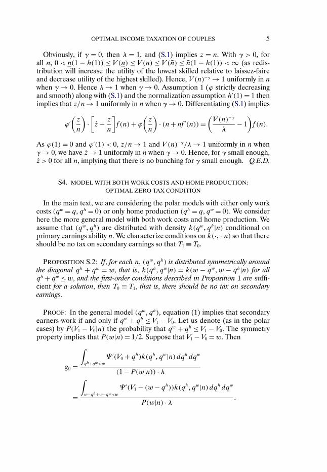
S4. MODEL WITH BOTH WORK COSTS AND HOME PRODUCTION:OPTIMAL ZERO TAX CONDITION

In the main text, we are considering the polar models with either only workcosts (qw = q�qh = 0) or only home production (qh = q�qw = 0). We considerhere the more general model with both work costs and home production. Weassume that (qw�qh) are distributed with density k(qw�qh|n) conditional onprimary earnings ability n. We characterize conditions on k(·� ·|n) so that thereshould be no tax on secondary earnings so that T1 ≡ T0.

PROPOSITION S.2: If, for each n, (qw�qh) is distributed symmetrically aroundthe diagonal qh + qw = w, that is, k(qh�qw|n) = k(w − qw�w − qh|n) for allqh + qw ≤w, and the first-order conditions described in Proposition 1 are suffi-cient for a solution, then T0 ≡ T1, that is, there should be no tax on secondaryearnings.

PROOF: In the general model (qw�qh), equation (1) implies that secondaryearners work if and only if qw + qh ≤ V1 − V0. Let us denote (as in the polarcases) by P(V1 − V0|n) the probability that qw + qh ≤ V1 − V0. The symmetryproperty implies that P(w|n) = 1/2. Suppose that V1 − V0 = w. Then

g0 =

∫qh+qw>w

Ψ ′(V0 + qh)k(qh�qw|n)dqh dqw

(1 − P(w|n)) · λ

=

∫w−qh+w−qw<w

Ψ ′(V1 − (w − qh))k(qh�qw|n)dqh dqw

P(w|n) · λ �

6 H. J. KLEVEN, C. T. KREINER, AND E. SAEZ

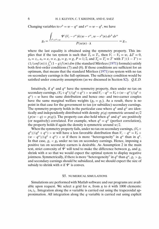
Changing variables to rh =w − qw and rw =w − qh, we have

g0 =

∫rh+rw<w

Ψ ′(V1 − rw)k(w − rw�w− rh|n)drh drw

P(w|n) · λ = g1�

where the last equality is obtained using the symmetry property. This im-plies that if the tax system is such that T0 ≡ T1, then V1 − V0 = w, T = 0,z0 = z1, ε0 = ε1 ≡ ε, g0 = g1 ≡ g, P = 1/2, and T ′

0 = T ′1 ≡ T ′ with T ′/(1 − T ′) =

(1/(εnf (n)))∫ n

n(1−g)f (m)dm (the standard Mirrlees (1971) formula) satisfy

both first-order conditions (7) and (8). If those conditions are sufficient for anoptimum, that means that the standard Mirrlees (1971) tax system with no taxon secondary earnings is the full optimum. The sufficiency condition would besatisfied under concavity assumptions (as we discussed in Section S2). Q.E.D.

Intuitively, if qh and qw have the symmetry property, then under no tax onsecondary earnings, (V0 +qh)/(qh+qw) > w and V1 −qw = V0 +(w−qw)/(qh+qw) < w have the same distribution and hence one- and two-earner coupleshave the same marginal welfare weights (g0 = g1). As a result, there is nopoint in that case for the government to tax (or subsidize) secondary earnings.The symmetry property holds in the particular case where qh and qw are iden-tically and independently distributed with density p(q) symmetric around w/2(p(w − q) = p(q)). The property can also hold when qh and qw are positively(or negatively) correlated. For example, when qh = qw (perfect correlation),the property holds if again the density is symmetric around w/2.

When the symmetry property fails, under no tax on secondary earnings, (V0 +qh)/(qh + qw) > w will have a less favorable distribution than V1 − qw = V0 +(w − qw)/(qh + qw) < w if there is more “heterogeneity” in qw than in qh.In that case, g1 < g0 under no tax on secondary earnings. Hence, imposing apositive tax on secondary earners is desirable. As Assumption 2 in the maintext, strict convexity of Ψ ′ will tend to make the difference between g0 and g1

shrink with n so that we would expect the optimal system to display negativejointness. Symmetrically, if there is more “heterogeneity” in qh than qw, g1 > g0

and secondary earnings should be subsidized, and we should expect the size ofsubsidy to shrink with n if Ψ ′ is convex.

S5. NUMERICAL SIMULATIONS

Simulations are performed with Matlab software and our programs are avail-able upon request. We select a grid for n, from n to n with 1000 elements:(nk)k. Integration along the n variable is carried out using the trapezoidal ap-proximation. All integration along the q variable is carried out using explicit

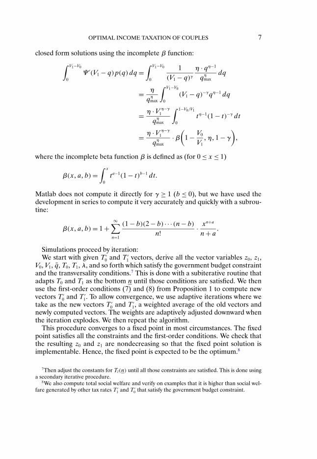
OPTIMAL INCOME TAXATION OF COUPLES 7

closed form solutions using the incomplete β function:∫ V1−V0

0Ψ ′(V1 − q)p(q)dq =

∫ V1−V0

0

1(V1 − q)γ

η · qη−1

qηmax

dq

= η

qηmax

∫ V1−V0

0(V1 − q)−γqη−1 dq

= η · V η−γ1

qηmax

∫ 1−V0/V1

0tη−1(1 − t)−γ dt

= η · V η−γ1

qηmax

·β(

1 − V0

V1�η�1 − γ

)�

where the incomplete beta function β is defined as (for 0 ≤ x≤ 1)

β(x�a�b)=∫ x

0ta−1(1 − t)b−1 dt�

Matlab does not compute it directly for γ ≥ 1 (b ≤ 0), but we have used thedevelopment in series to compute it very accurately and quickly with a subrou-tine:

β(x�a�b)= 1 +∞∑n=1

(1 − b)(2 − b) · · · (n− b)

n! · xn+a

n+ a�

Simulations proceed by iteration:We start with given T ′

0 and T ′1 vectors, derive all the vector variables z0, z1,

V0, V1, q, T0, T1, λ, and so forth which satisfy the government budget constraintand the transversality conditions.7 This is done with a subiterative routine thatadapts T0 and T1 as the bottom n until those conditions are satisfied. We thenuse the first-order conditions (7) and (8) from Proposition 1 to compute newvectors T ′

0 and T ′1. To allow convergence, we use adaptive iterations where we

take as the new vectors T ′0 and T ′

1, a weighted average of the old vectors andnewly computed vectors. The weights are adaptively adjusted downward whenthe iteration explodes. We then repeat the algorithm.

This procedure converges to a fixed point in most circumstances. The fixedpoint satisfies all the constraints and the first-order conditions. We check thatthe resulting z0 and z1 are nondecreasing so that the fixed point solution isimplementable. Hence, the fixed point is expected to be the optimum.8

7Then adjust the constants for Tl(n) until all those constraints are satisfied. This is done usinga secondary iterative procedure.

8We also compute total social welfare and verify on examples that it is higher than social wel-fare generated by other tax rates T ′

1 and T ′0 that satisfy the government budget constraint.

8 H. J. KLEVEN, C. T. KREINER, AND E. SAEZ

The central advantage of our method is that the optimal solution can beapproximated very closely and quickly. In contrast, direct maximization wherewe search the optimum over a large set of parametric tax systems by computingdirectly social welfare would be much slower and less precise.

REFERENCES

KLEVEN, H. J., C. T. KREINER, AND E. SAEZ (2007): “The Optimal Income Taxation of Couplesas a Multi-Dimensional Screening Problem,” Working Paper 2092, CESifo.

MACKI, J. (1982): Introduction to Optimal Control Theory. New York: Springer-Verlag.MANGASARIAN, O. L. (1966): “Sufficient Conditions for the Optimal Control of Nonlinear Sys-

tems,” Journal of SIAM Control, 4, 139–152.MIRRLEES (1971): “An Exploration in the Theory of Optimal Income Taxation,” Review of Eco-

nomic Studies, 38, 175–208.

Dept. of Economics, London School of Economics, Houghton Street, LondonWC2A 2AE, U.K. and Economic Policy Research Unit, Dept. of Economics, Uni-versity of Copenhagen, Copenhagen, Denmark and Centre for Economic PolicyResearch, London, U.K.; h.j.kleven@lse.ac.uk,

Dept. of Economics, University of Copenhagen, Studiestraede 6, 1455 Copen-hagen, Denmark and Economic Policy Research Unit, Dept. of Economics, Uni-versity of Copenhagen, Copenhagen, Denmark and CESifo, Munich, Germany,

andDept. of Economics, University of California–Berkeley, 549 Evans Hall 3880,

Berkeley, CA 94720, U.S.A. and NBER; saez@econ.berkeley.edu.

Manuscript received August, 2007; final revision received August, 2008.