The Occupations and Human Capital of U.S. Immigrants · employment across Census-level occupations...

The Occupations and Human Capital of U.S.

Immigrants∗

Todd Schoellman †

June, 2008

Abstract

Foreign-born workers accounted for as little as 0.5% and as much as 45% of total

employment across Census-level occupations in the year 2000. This paper estimates

the effects of immigration on the distribution of wages and employment for American-

born workers employed across this range of occupations. A model of labor markets

is proposed where workers from different countries vary in their endowment of a

multi-dimensional vector of human capital. I use data on the occupational choices

of workers and the skill requirements of Census occupations to estimate the human

capital endowments of immigrants from 130 different countries. Compared to Amer-

icans, immigrants are relatively abundant in cognitive ability and physical skills, but

relatively scarce in communication skills. I then estimate the effect of removing im-

migrants from the U.S., allowing for a general equilibrium reallocation of American

workers and capital across occupations. The distribution of wage effects is highly

skewed: the largest wage decrease is just 1.5%, but a few occupations have wage

increases as high as 64%. The median of the absolute value of wage changes is just

0.6%. The evidence suggests that most (but not all) Americans are able to respond

to immigration by substituting into similar occupations that are intensive in com-

munications, experience, or training, and experience only small wage changes. The

differential effects of low and high-skilled immigration are also estimated.

∗Thanks to Curtis Simon, Kevin Murphy, and the Bag Lunch participants at Clemson University forhelpful comments on early work, and to Tom Mroz for generous advice and use of computational resources.The usual disclaimer applies.†Address: John E. Walker Department of Economics, Clemson University, Clemson, SC 29642. E-mail:

[email protected].

1

1 Introduction

Immigrants to the United States tend to concentrate into certain occupations. For instance,

they account for as little as 0.5% and as much as 45% of total employment across 453 Census-

level occupations in the year 2000. Two conflicting popular narratives for this concentration

are that immigrants take jobs Americans don’t want, or that immigrants drive down wages

and push Americans out of jobs. This paper explores the effects of immigration on the

distribution of wages and employment across occupations.

To make progress in these distributional questions, it is important to understand two

points: why immigrants select the occupations that they do; and how effectively Americans

can substitute out of occupations that see an influx of immigrant workers. This paper pro-

poses that the way to understand both of these issues is through the lens of human capital.

It develops a theory of labor markets similar to recent work by Lazear (2003). Human

capital is a vector of different attributes, such as physical skills and education, rather than

a scalar. Workers have heterogeneous endowments over possible combinations of human

capital: some are educated and clumsy, educated and nimble, and so on. Occupations all

use capital and labor hours in the same fashion, but vary in how they combine the human

capital vector into output. Some occupations are physical skill-intensive, while others are

education-intensive. In equilibrium, workers tend to choose occupations intensive in the

skills that they possess abundantly.

In this model, an immigrant is someone whose human capital is different from an Ameri-

can (or whose human capital is drawn from a different distribution than that of Americans).

Human capital differences can come from differences in environment (such as school qual-

ity) or from the selection process that determines who immigrates, but the source is not

important. What is important is that human capital differences explain differences in oc-

cupational choices between immigrants and Americans.

Estimates of human capital are needed to conduct counterfactual simulations and ex-

plore the role of immigration on wage distributions. For some of the elements of human

capital the Census provides direct information (e.g. education), but for others it does not

(e.g. physical skills, cognitive ability). Instead of using the direct but limited information

on human capital, this paper uses an indirect measurement approach. It constructs infor-

mation on the skill intensity of occupations and on the occupation choices of workers by

country of birth. With these two pieces of information it then infers the human capital of

workers that is consistent with their observed occupational choices.

2

Data on occupational choices are taken from the 5% sample of the 2000 U.S. Census

PUMS, which provides information on the choices of immigrants from 130 countries over

453 occupations. I construct data on the skill intensity of occupations using the O*Net

Database, which includes a wealth of information on the tasks, skills, abilities, and activities

of occupations and the workers in those occupations. I use this information to measure

the skill-intensity of occupations along five dimensions of human capital: education and

learned knowledge, training and experience, cognitive abilities, physical skills, and language

and communication skills. Information on the characteristics of occupations has been used

elsewhere to measure the specificity or generality of skills to occupations (Spitz-Oener 2006,

Gathmann and Schonberg 2006) and the effects of computerization on workers (Autor, Levy,

and Murnane 2003). Perhaps the most similar paper to mine is Peri and Sparber (2007),

which uses task information to characterize occupations as being manual or interactive.

They demonstrate that low-skilled immigrants specialize in the former while American-born

workers specialize in the latter, so that they are much less substitutable than is commonly

thought.

Empirical implementation yields estimates of the human capital of workers from 130

different countries along the 5 skill dimensions, all relative to the average American. Where

Census data provide direct measures of human capital, the direct and indirect measures are

highly correlated; but indirect measurement also provides estimates of the human capital

endowments of difficult to observe attributes such as cognitive ability. In general, most

immigrants have more cognitive ability but less communication skills than the average

American. Immigrants from developed countries tend to have more experience and training,

while immigrants from developing countries tend to be abundant in physical skills.

To estimate the effect of immigrants on the distribution of wages and employment by

Americans, I simulate two counterfactual general equilibrium outcomes, corresponding to an

equilibrium with all immigrants removed, and an equilibrium with low-skilled immigrants

removed. I proxy low-skilled immigrants as immigrants from the fifteen countries with

the highest rates of estimated illegal immigration. These simulations allow for general

equilibrium reallocations of capital and workers across occupations. The extent to which

workers substitute across occupations is governed by two factors. First, there is an aggregate

elasticity of substitution between the outputs of different occupations, which determines

how easily legal services can be substituted for medical services in producing the final

aggregate consumption good. Second is the technological similarity of the two occupations;

workers are more willing to substitute between technogically similar occupations such as

3

physicist and engineer because their marginal product and hence wages will be similar in

the two occupations.

I compare wages and employment across the actual and the two simulated economies.

The central finding of the paper is that immigration makes a small difference in the wages

of most workers, but a large difference for a few occupations. A majority of occupations

see a wage change of less than 1% in all simulated cases. The distribution of wage changes

is highly skewed: excluding immigrants lowers wages by at most 2% in any occupation,

but increases wages by as much as 64% in a few occupations. The size of wage gains is

determined by how the occupation’s technological intensity matches up with immigrants’

skills, and the presence of nearby substitutes. In particular, since all immigrants are scarce

in communication skills, and low-skilled immigrants are scarce in experience and training,

occupations intensive in these skills do well from immigration. Workers in these occupations,

or workers who can easily substitute into these occupations, likewise do well. The fact that

most wage changes are small suggests that most workers find it easy to substitute into such

an occupation.

There is a large related literature on the effects of immigrants on wages, but most

previous studies focus on effects on aggregate wages, or on a world with two types of

workers, skilled and unskilled. This paper is most closely related to three previous studies.

Ottaviano and Peri (2006) shares a general equilibrium framework with capital. They note

that the effect of immigration on wages differs in the short run (when the capital stock

is fixed) and the long run (when capital is free to adjust). This paper embeds an even

longer view of the long run, where capital and occupations are both free to adjust. Peri

and Sparber (2007) shows that immigrants specialize in manual occupations and suggests

that this may limit competition by immigrants, which is mirrored here by the ability of

Americans to substitute into communications-intensive occupations when they are available.

However, I find that for some occupations no effective substitute is available, so Americans

with tastes or skills suitable to those occupations face large wage losses from immigration.

Borjas (2005) studies the relationship between foreign-student enrollment in U.S. doctoral

programs and wages paid to the graduates of those programs. Broadly speaking, his results

suggest that immigrants have sorted into degree programs that are relatively less intensive in

communications (such as physics instead of sociology) and depressed relative wages of those

programs, which is similar to the effect predicted for engineering and science occupations

in this paper.

The paper proceeds as follows. Section 2 presents the model. Section 3 illustrates the

4

main properties of the model and the assumptions under which it is estimable. Section 4

introduces the data and estimates the human capital endowments of immigrants. Section

5 conducts the experiments using measured skills. Section 6 concludes.

2 A Model of Labor Markets with Vector Human Cap-

ital

2.1 Occupations and Human Capital

The model is a static representation of labor markets. Human capital H is an array of S

elements, H = (h1, h2, ..hS), with a representative element indexed by hs. Each s denotes

a specific type of human capital, which I call a skill, although it may also include abilities,

training, or any of the other common notions of human capital. For instance, a common

specification would be S = 2, with human capital consisting of physical and mental abilities.

Human capital endowments are defined on (0,∞)S.

There are J occupations in the economy, indexed by j. Each occupation utilizes all

of the available skills of workers, but occupations vary in how intensively they use each

of the skills. An occupation is characterized by a set of technological parameters (ωjs)Ss=1.

The effective labor input of a worker with human capital H who works nj(H) hours in

occupation j is given by:

nj(H)ΠSs=1(hs)

ωjs

Skill endowments can be greater than or less than 1. For hs > 1, workers are more produc-

tive in higher ωjs occupations; for hs < 1, they are less productive.

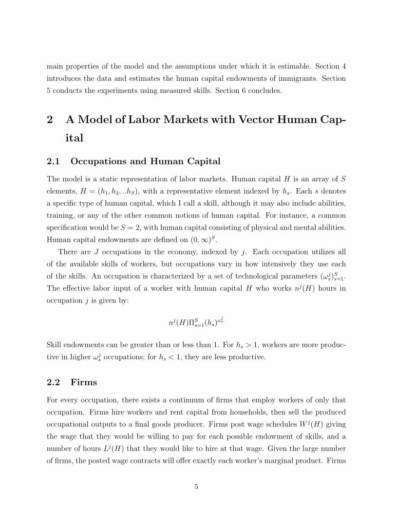
2.2 Firms

For every occupation, there exists a continuum of firms that employ workers of only that

occupation. Firms hire workers and rent capital from households, then sell the produced

occupational outputs to a final goods producer. Firms post wage schedules W j(H) giving

the wage that they would be willing to pay for each possible endowment of skills, and a

number of hours Lj(H) that they would like to hire at that wage. Given the large number

of firms, the posted wage contracts will offer exactly each worker’s marginal product. Firms

5

also take the rental price of capital R as given and rent a quantity Kj(H) of capital for each

type of worker. Firms find it optimal to vary capital allocated to workers with different

levels of human capital.

Output Y j(H) of workers H in occupation j is the usual Cobb-Douglas aggregate over

capital Kj(H), effective labor input, and labor-augmenting technology A that is general

across occupations. Firms choose capital and hours for each skill type to maximize profits

per skill type:

P j(Kj(H))α(ALj(H)ΠSs=1(hs)

ωjs)1−α −RKj(H)−W (H)Lj(H) (1)

The first-order conditions are given by:

P jαY j(H)

Kj(H)= R

P j(1− α)Y j(H)

Lj(H)= W (H)

P j(1− α)ωjsY j(H)

hs=∂W (H)

∂hsLj(H)

There is a single price-taking final goods producer. The producer faces prices P j and

purchases quantities of occupational outputs Xj. It aggregates the occupational outputs

using a CES production function with elasticity of substitution ψ. It sells its output Y to

consumers for consumption. I normalize the price of the final good to be the numeraire of

the economy. Then the final goods producer maximizes profits:

[J∑j=1

(Xj)1−1/ψ

]ψ/(ψ−1)

−J∑j=1

XjP j (2)

The usual CES relative demand conditions apply here:

Xj

Xj′=

(P j

P j′

)−ψ(3)

2.3 Workers

Workers have additively separable preferences over consumption and time spent in the labor

market. Their preferences over consumption c are given by a standard CRRA function.

6

Their preferences over time spent in the labor market depend on hours of work and the

occupation where those hours are worked. Thus, the disutility of a forty-hour workweek may

vary depending on whether the forty hours are spent working as a lawyer or a landscaper.

These preferences are specific to the worker. I denote by εj the idiosyncratic preference of

a worker for occupation j.

Workers have two forms of heterogeneity: in their skill endowments, H, and in their

preferences for occupations ε = (εj)Jj=1. I describe a worker by her skills and preferences,

(H, ε), so c(H, ε) is the consumption of such a worker, and so on. (H, ε) is a random draw

from a joint distribution with pdf ξ(H, ε) and cdf Ξ(H, ε) which is defined on (0,∞)S ×(0,∞)J . I assume that both ξ and Ξ are integrable and well-behaved so that expected

utility exists; in the next section I restrict ξ so that this is true.

Given a worker’s skill endowment and her draw of occupational preferences, her utility

function is given by:

U(H, ε) =c(H, ε)1−1/σ

1− 1/σ− log

(J∑j=1

nj(H, ε)

εj

)(4)

Workers are also endowed with a(H) units of capital. Their income comes from renting

out their endowment of capital at rate R and from their wages∑J

j=1wj(H)nj(H, ε). They

spend their income on consumption, c(H, ε), so their budget constraint is:

c(H, ε) = Ra(H) +J∑j=1

wj(H)nj(H, ε) (5)

Workers choose consumption, hours worked, and occupations to maximize their utility,

subject to their budget constraint and the time restriction∑J

j=1 nj(H, ε) ≤ N . One key

feature of the problem is that the log preferences guarantee the choice of a unique occupation

that depends only on wage offers and occupational tastes ε.

Proposition 1 – Independence of Occupational Choice

The workers’ choice problem can be analyzed in two separate pieces. First, they choose the

occupation that maximizes wj(H)εj. Second, they choose consumption and hours, which are

independent of their taste realizations ε.

Proof: Combine the FOC for consumption and hours worked to find that for occupations

7

with positive hours:

J∑j=1

nj(H, ε)

εj=c(H, ε)1/σ

wj(H)εj

with nj = 0 otherwise. As long as ξ is continuous, this equation will hold for only one

occupation. Then substitute into equations (4) and (5) to find the equivalent problem:

max U(H, ε) =(c(H, ε))1−1/σ

1− 1/σ− 1

σlog(c(H, ε)) + log(wj(H)εj)

s.t. c(H, ε)− (c(H, ε))1/σ = Ra(H)

s.t.J∑j=1

nj(H, ε) ≤ N

The only term that depends on occupational choice is log(wj(H)εj). The optimal c(H, ε)

is independent of ε, and by the first-order conditions, so too is n(H, ε). QED

For the rest of the paper, I omit the irrelevant ε when possible, using only c(H). Hours

worked n(H) also does not vary with tastes ε, but the occupation chosen does. I let

dj(H, ε) be an indicator function taking a value of 1 if worker (H, ε) chooses occupation j,

and taking 0 otherwise. Given the functional form of this equivalent problem, εj represents

the compensating wage differential across occupations. If a worker’s draw εj for lawyer is

twice that of her draw for fire fighter, her wage as a fire fighter needs to be twice her wage

as a lawyer to make her indifferent between the two occupations.

2.4 Equilibrium

There are four sets of market clearing conditions for this economy: one condition for output,

one condition for capital, one condition for each of the occupational goods markets, and

8

one condition for each type of human capital. They are given by:

Y =

∫ ∫c(H)ξ(H, ε)dHdε (6)

Xj =

∫ ∫Y j(H)ξ(H, ε)dHdε ∀j (7)

J∑j=1

∫Kj(H)dH =

∫ ∫a(H)ξ(H, ε)dHdε (8)

Lj(H) =

∫n(H)dj(H, ε)ξ(H, ε)dε ∀H (9)

An equilibrium in this economy is a set of prices (P j, R,W (H)), allocations for the work-

ers, (c(H), n(H), dj(H, ε), allocations for intermediate goods firms, (Kj(H), Lj(H), Y j(H)),

and allocations for the final goods producer (Y,Xj) that satisfy the following conditions:

1. Taking prices as given, workers maximize their utility (4) subject to their budget

constraint (5) and time restriction∑J

j=1 nj(H) ≤ N .

2. Taking prices as given, intermediate firms maximize profits, (1).

3. Taking prices as given, the final goods producer maximizes profits, (2)

4. Markets clear, (6) - (9).

3 Equilibrium Predictions

The model of labor markets here is similar to the Heckscher-Ohlin theory of trade (Heckscher

1949, Ohlin 1933). Workers vary in their endowment of skills, and have access to a number

of occupations that vary in their skill intensity. I show that a pseudo-Rybczynski Theorem

holds: workers who are more s-abundant have a higher probability of choosing occupations

that are s-intensive, when s-intensity is appropriately defined. Introducing idiosyncratic

tastes is not only realistic, but also convenient because it makes choices continuous in

endowments and the results easier to characterize.

9

3.1 Allocation of Workers to Occupations

In equilibrium, the wage offered to worker H if she chooses occupation j is given by:

W j(H) =(P j)1/(1−α)

Rα/(1−α)αα/(1−α)(1− α)AΠS

s=1(hs)ωj

s (10)

Workers choose the occupation j that maximizes the product of wages and the idiosyn-

cratic preference for occupation j. I respecify this as maximization in logs for convenience:

log(wj(H)εj) = log

(A(1− α)αα/(1−α)

Rα/(1−α)

)+

1

1− αlog(P j) +

S∑s=1

ωjs log(hs) + log(εj)

The model can be estimated under a variety of assumptions on ξ(H, ε). However, two

assumptions are particularly helpful in making the estimation computationally tractable.

First is an assumption over the joint distribution:

Assumption 1 – Independence of Tastes and Endowments

The distribution ξ(H, ε) can be decomposed into two independent marginal distributions,

f(H) and g(ε), with F and G as the corresponding CDF’s.

Note that this assumption does not rule out skill endowment affecting occupational choice.

It merely constrains the effects to come through the wage channel. This assumption can be

relaxed; intuitively, as long as workers are more likely to choose occupations in which they

are more productive, then the estimation used here will be able to infer their productivities.

Whether they choose that occupation because they value high wages or because they derive

non-pecuniary satisfaction out of being good at their occupation is less critical.

The second assumption is over the functional form of the idiosyncratic preferences:

Assumption 2 – Distribution of Preferences

εj is distributed i.i.d according to the Type-2 Gumbel distribution or, equivalently, log(εj)

is distributed i.i.d according to the Type-I extreme value distribution.

Assumptions 1 and 2 are used mostly to make estimation computationally practical, al-

though they are also useful for deriving clean propositions about the model. The extreme

value distribution means that this problem fits into the probablistic choice framework of

McFadden (1974). It is amenable to estimation using various logit methods; I consider the

conditional and mixed logit approaches in the next section. Logit models are well-known

10

to be more practical than alternatives such as multinomial probits for estimating data sets

with large sample size and a large number of variables; I have both. Under Assumptions 1

and 2, the probability that a worker chooses occupation j′ conditional on human capital H

is given by:

q(j′|H) =exp

[1

1−α log(P j′) +∑S

s=1 ωj′s log(hs)

]∑J

j=1 exp[

11−α log(P j) +

∑Ss=1 ω

js log(hs)

] (11)

Cancelling out the log and exponential terms, the probability that a worker chooses

occupation j is merely the wage that she would earn in occupation j, divided by the

sum of the wages she could earn in each possible occupation. By a usual law of large

numbers argument, q(j′|H) also represents the fraction of workers with endowment H who

choose occupation j′. One convenient result of using the logistic framework is that it is

straightforward to give the comparative statics results. For this model the key comparative

static is how changes in a worker’s skill abundance affects her probability of matching in

each of the J occupations.

Proposition 2 – Psuedo-Rybczynski Theorem

A marginal increase in log(hs) makes a worker more likely to work in occupations that are

more s-intensive than the expected local alternative and less likely to work in occupations

that are less s-intensive than the expected local alternative.

The proposition comes directly from the usual marginal effects equation in a conditional

logit model.1 It is the analogue to the Rybczynski Theorem from trade: an increase in s-

abundance makes a worker more likely to choose s-intensive occupations. With multiple

choices and idiosyncratic preferences, an occupation is s-intensive if its intensity parameter

ωjs is higher than the probability-weighted local alternative for a given worker.

An important and related question is what would happen to wages and occupational

choices if all workers became more s-abundant. Proposition 2 is inherently partial equilib-

rium, so it offers little guidance to these questions. In the next section, I provide a general

equilibrium result.

1The exact equation is ∂q(j′|H)∂ log(hs) = q(j′|H)

[ωj′

s −∑J

j=1 ωjsq(j|H)

]

11

3.2 Prices and Wages in General Equilibrium

The wages offered to workers who choose two different occupations will in general depend on

the prices offered for the output of those occupations, as can be seen by equation (10). Prices

are determined in general equilibrium to allocate labor across occupations in a way that

is consistent with the CES demand equation of the final goods producer (3). The primary

determinant of the prices is the abundance of different types of skills. Relative prices (and

hence relative wages) are inversely proportional to a weighted average of effective human

capital:

P j

P j′=

E[n(H)ΠS

s=1h2ωj

ss

]E[n(H)ΠS

s=1h2ωj′

ss

]−(1−α)/((ψ−1)(1−α)+2)

(12)

A more straightforward way to see the effect of a reallocation of the distribution of

labor across skill types for relative prices is to consider the comparative static of marginal

changes in the density:

Proposition 3 – Skill Abundance and Prices

If workers with human capital H are a higher proportion of labor input for occupation j

than occupation j′, then an increase in the abundance of those workers f(H) decreases the

price and wages of j relative to j′.

Proof: The comparative static of relative prices (and hence relative wages) with respect

to density f(H) is:

∂ P j

P j′

∂f(H)=(−1)

1− α(ψ − 1)(1− α) + 2

E[n(H)ΠS

s=1h2ωj

ss

]E[n(H)ΠS

s=1h2ωj′

ss

]−(1−α)/((ψ−1)(1−α)+2)−1

×

E[n(H)ΠS

s=1h2ωj′

ss

]n(H)ΠS

s=1h2ωj

ss − E

[n(H)ΠS

s=1h2ωj

ss

]n(H)ΠS

s=1h2ωj′

ss

E[n(H)ΠS

s=1h2ωj′

ss

]2The sign of the whole expression depends on the sign of:

ΠSs=1h

2ωj′s

s

E[n(H)ΠS

s=1h2ωj′

ss

] − ΠSs=1h

2ωjs

s

E[n(H)ΠS

s=1h2ωj

ss

]

12

QED.

An increase in the abundance of immigrants abundant in a particular skill will lower

the relative wages of occupations intensive in that skill.

3.3 An Application to Immigrants

To apply this framework to immigrants, I examine the distribution of skills conditional on

country of origin. Let f(H|i) denote the distribution of skills for a worker who was born

in country i and ηi denote the fraction of the U.S. labor force born in country i, i = 1..I.

If H were observed, then q(j′|H) is given by equation (11). Since only i is observed, it is

necessary to study the conditional probability q(j′|i) by integrating over all possible human

capital realizations:

q(j′|i) =

∫q(j′|H)f(H|i)d(H) (13)

This equation has the general form of a mixed logit. To proceed, I assume that f(H|i) is

given by a particular distribution with a limited set of parameters θi that vary by country.

The prices can be estimated as occupation fixed effects. Then given data on the skill-

intensity of occupations ω, the mixed logit allows me to estimate the parameters θi.2 In

the next section I introduce the data and estimate f(H|i) under two different assumptions

about the possible form of the conditional distribution.

4 Empirical Strategy

The empirical strategy is to construct indirect measures of human capital of workers condi-

tional on country of origin. To do so, I construct measures of skill intensity of occupations

using occupational task data, and take from Census data the occupational choices of work-

ers. I can then infer the human capital endowments of workers from their occupational

choices. For some forms of human capital, I have limited measures of skill endowment

available. Hence, one route is to test the indirect measuremetn of human capital against

direct measurement. I pursue this in Section 4.2. However, for most skills of interest there

is little or no available data on the endowments of workers. Here I proceed by assuming

2Useful information about the issues in estimating a mixed logit can be found in Train (2003) andHensher and Greene (2001).

13

that theory is true, and estimating the human capital endowments that are consistent with

the theory and the observed occupational choices of immigrants from different countries.

4.1 Data

The data for this project are taken from two sources. I gather data on the occupations

and characteristics of immigrants from the 5% sample of the 2000 U.S. Census, drawn

from the IPUMS-USA system (Ruggles, Sobek, Alexander, Fitch, Goeken, Hall, King, and

Ronnander 2004). The Census asks every respondent to list their country of birth. For pri-

vacy reasons, it aggregates this data so that no birthplace with fewer than 10,000 reported

immigrants is reported separately. After aggregation, there are observations for I = 131

different birthplaces, including the United States. Some of the birthplaces are nonstan-

dard; for instance, there are response categories for Czechoslovakia, the Czech Republic,

and Slovakia, since immigrants may have departed before or after the split. I preserve

every statistical entity which is separately identified, and refer to them as countries as a

shorthand.3

I focus on immigrants that enter the United States after making some of their most im-

portant human capital decisions. In particular, I use an imputation rule based on reported

education, age, and year of immigration to retain only workers who are very unlikely to

have received any U.S. education. This restriction is especially helpful for the experiments:

immigrants who acquire much of their human capital in the United States are less likely

to be meaningfully different from Americans, have different distributional implications for

American-born workers, and are a less useful signal of the human capital conditions of their

country’s non-migrants. I also include only those who worked in the previous year and are

aged 16-65. The Census provides information on the occupation of workers based on the

Standard Occupation Classification (SOC) system, with some idiosyncratic modifications.

Overall, the Census version of SOC includes 476 occupations.

Data on the underlying characteristics of occupations are derived from the O*NET

database version 12.4 The O*NET database project is the continuation of occupational

characteristic descriptions that used to be provided in the Dictionary of Occupational Ti-

3There are two exceptions to this policy. First, I merge the United Kingdom together; second, I excludeNorth Korea, the USSR, and Russia, since it is not possible to identify them separately from other countries.The count of 131 already includes these reductions in sample size.

4Occupational Information Network (O*NET) and US Department of Labor/Employment and TrainingAdministration (USDOL/ETA) (2007).

14

tles (DOT), which was last updated in 1991 (U.S. Department of Labor, Employment, and

Training Administration 1991). The database includes information on the worker character-

istics, worker requirements, experience requirements, occupational requirements, workforce

characteristics, and other occupation-specific information for the occupations in the SOC

classification system. The database contains a wealth of information, and it is necessary

to compact the information along two dimensions. First, the O*NET Database includes

unique information on 812 occupations. For privacy reasons, the Census aggregates over

many occupation codes for which there are too few observations; they give information

on how the categories are merged, which I use to construct a crosswalk. For instance, the

Census aggregates mathematicians, statisticians, and miscellaneous mathematical scientists

into a single occupation. I have no information on the relative employment of mathemati-

cians or statisticians, so I take the simple average of the underlying characteristics. For a

few occupations the O*NET database does not have all the necessary information, and for a

handful the concordance between Census codes and O*NET database codes is not entirely

straightforward; I exclude these categories. Then there are 452 remaining occupations.

Second, the database scores occupations on over 250 dimensions, an unwieldy amount

of information for analytical purposes. I use three principles to pare this information into

meaningful measures of a few critical skills. First, I use information that corresponds

most closely to measures of deep technological parameters. This principle rules out several

categories of information (such as worker interests) and a fair number of specific dimensions

(such as “exposure to disease” or “operating vehicles activities”). Second, I choose skills

for which I will measure skill intensity and estimate skill endowments. The five skills

are: education and learned knowledge, training and experience, cognitive abilities, physical

skills, and language and communication skills. Third, for each skill I choose a small subset

of dimensions that correspond most closely to technological intensity for that skill, and I

use principal component analysis (PCA) to aggregate the many dimensions into a single

numerical measure of technological intensity. I then scale each of the measures to lie on

the unit interval, with the least intensive occupation for each category rescaled as 0 and

the most intensive as 1. Appendix A provides further detail on exactly what underlying

dimensions were used. It also provides the three highest and lowest-scoring occupations for

each skill, which may be a useful check.

I am sensitive to the criticism that with such a wealth of information at hand, there are

many possible skills to estimate and many possible ways to construct the indices for skills.

I view this exercise as a useful starting point in using this extremely rich data source. Each

15

of the five skills is a relatively commonly discussed component of human capital. They are

also particularly applicable when studying immigrants. A common finding in the literature

on the occupations of immigrants is that immigrants tend to come from the two tails of

the skill distribution (Ottaviano and Peri 2006). This finding corresponds to a trade-off

between physical skills and cognitive ability or education. Cognitive ability is also important

in discussing immigrant selection. Communication is of interest given the large language

barrier that many immigrants face. Finally, experience and training are important for the

purpose of measuring the transferability of skills across countries.5

Hence, while alternative choices are possible and potentially interesting, I view this

method of exploring the technological intensity of occupations and skills of workers along

these five dimensions as a useful step for human capital measurement. Before estimating the

model, I provide some preliminary evidence that the constructed skill intensity measures

and the model are plausible.

4.2 Checks on Intensity Measures

According to Proposition 2, workers who are more s-abundant should choose occupations

that are s-intensive. Here, I perform a preliminary, joint test of the model and the measures

of skill intensity. The Census provides some proxies for the skill endowments of workers. I

thus test whether there is an observed correlation between abundance in these proxies for

skill endowment and the skill intensity of the worker’s chosen occupation. I implement this

by regressing:

ωjs = b1 + b2hs + e

where ωjs is the constructed skill intensity of the worker’s chosen occupation and hs is the

proxy for skill endowment. I then test whether b2 > 0.

For each of the skills I construct a proxy for abundance. Educational attainment is

5One common alternative would be to include all the variables in a large PCA analysis and extractthe first n components. However, there is a problem with interpretability of the results. For instance,a common component from such an analysis relates caring for others, exposure to disease, knowledge ofbiology and chemistry, and advanced college education requirements. These characteristics describe a poolof occupations (doctor, nurse) and not a set of related, deep technologies. In general, PCA cannot sortout factors that tend to be correlated because they are manifestations of a single technological parameter,and factors that tend to be correlated because many occupations have similar skill requirements. For thepurposes of this estimation I want to separate the two: are there so few Mexican doctors because of theeducation requirements, the communication requirements, or the training requirements? Doing so requiresimposing priors as I have done here.

16

Table 1: Check on Measured Skill Intensity

Skill Dimension Estimated b2a t-stat

Education/Knowledge 0.431 299

Experience/Training 0.0018 339

Cognitive 0.068 195

Physical −0.062 94

Communication 0.195 320a For experience and training b2 is the marginal effect

of an additional year of potential experience. For allother variables it is the estimate of the highestcategory, with the lowest category omitted.

a straightforward indicator of education and knowledge. Likewise, the Census includes a

measure of self-assessed English language proficiency, which I use as a measure of com-

munication skills. The other dimensions are more limited. I use potential experience as

a measure of experience and training. The Census also includes three dummy variables

on disability status: I use (lack of) vision or hearing disability as a measure of physical

skills, and (lack of) difficulty remembering as a measure of cognitive skills. I use the same

sample as for the previous section. For the tests other than communication, I use only

Americans to avoid complications such as comparing Swedish and Kenyan education; for

communication, I use only foreign-born workers.

Table 1 gives the results. With the large sample, every variable is statistically significant.

For communication and education, the effect is also large: these are the two best proxy

measures.6 All the coefficients have the right sign except for physical disability. This

sign may be due to a reverse causality problem: workers with more physically demanding

occupations may also be more likely to suffer disabilities from their work.

From these tests I conclude that the constructed measures of skill intensity and the

theoretical predictions are reasonable. However, the data limitations for information on

the skills of workers is binding. In the next two sections, I use the theory to back out the

implied skill endowments.

6The coefficient for communication survives controlling for birthplace or using only Mexican immigrants(the largest single group), although both changes cut its impact by about half.

17

4.3 Estimation as a Conditional Logit

To estimate equation (13), I impose further structure on the possible functional forms of

the conditional distribution f(H|i). The simplest assumption would be that the conditional

distribution has a degenerate distribution placing all the mass on a single point, with that

point differing by country of origin. Then all workers born in country i have the same skills.

Assumption 3 – Point Distribution of Skills

f(H|i) = 1 if H = H i; f(H|i) = 0 otherwise.

Under this condition equation (13) simplifies to:

q(j′|i) =exp

[1

1−α log(P j′) +∑S

s=1 ωj′s log(his)

]∑J

j=1 exp[

11−α log(P j) +

∑Ss=1 ω

js log(his)

]This function has the form of the conditional logit as introduced by McFadden (1974). As

is standard for a conditional logit, it is not possible to estimate a full set of prices and skill

endowments because of collinearity. However, I can identify a set of related parameters:1

1−α log(P j)+∑S

s=1 ωjs log(hUSs ) for each occupation, and log(his)−log(hUSs ) for every country

and skill. Note that the second set of estimated parameters is the log of the skill ratio

between the average immigrant and the average American, which is exactly the object of

interest. It is possible to separately identify each of the relevant parameters by imposing

the restrictions of the general equilibrium model, but it does not facilitate interpretation

of the empirical results. Hence, I delay doing so until Section 5. Additionally, I restrict1

1−α log(P 452) +∑S

s=1 ω452s log(hUSs ) = 0. The choice of numeraire has already pinned down

prices, so this normalization pins down the level of A.

The estimates are presented in Table 4, along with their statistical significance and the

number of observations for each country. Rather than discussing each of the 650 relative skill

endowments separately, I identify broad trends. I am interested in how immigrants compare

to Americans in general, and in differences across immigrant groups by the development

status of their source country. A useful summary of the trends is given graphically in Figures

1 and 2. These figures are scatter plots of the estimated log skill difference against PPP

GDP p.c. in the source country for each of the five skills, for each country for which data

is available.7 Figure 1 contains the communication skills, cognitive ability, and education,

7PPP GDP p.c. from the World Development Indicators (World Bank 2006).

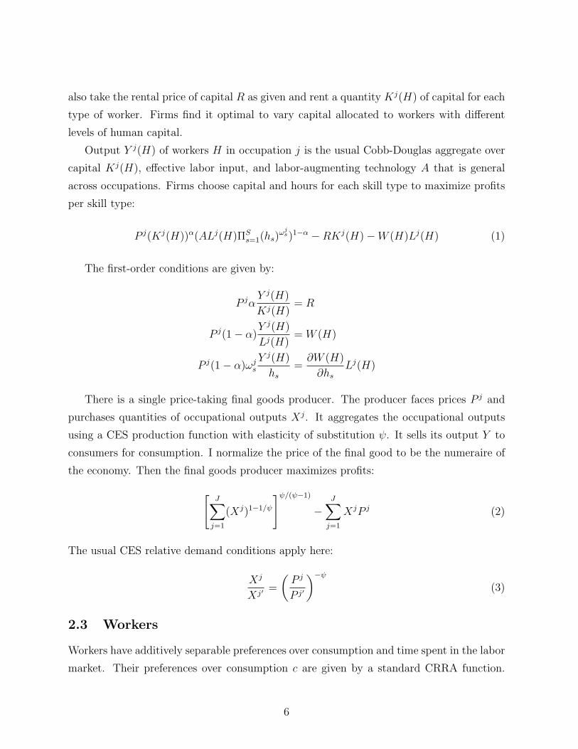
18

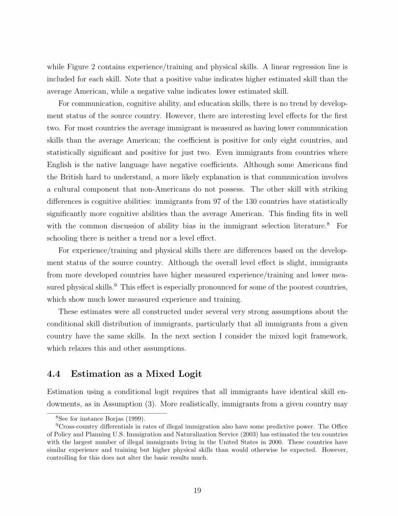
while Figure 2 contains experience/training and physical skills. A linear regression line is

included for each skill. Note that a positive value indicates higher estimated skill than the

average American, while a negative value indicates lower estimated skill.

For communication, cognitive ability, and education skills, there is no trend by develop-

ment status of the source country. However, there are interesting level effects for the first

two. For most countries the average immigrant is measured as having lower communication

skills than the average American; the coefficient is positive for only eight countries, and

statistically significant and positive for just two. Even immigrants from countries where

English is the native language have negative coefficients. Although some Americans find

the British hard to understand, a more likely explanation is that communication involves

a cultural component that non-Americans do not possess. The other skill with striking

differences is cognitive abilities: immigrants from 97 of the 130 countries have statistically

significantly more cognitive abilities than the average American. This finding fits in well

with the common discussion of ability bias in the immigrant selection literature.8 For

schooling there is neither a trend nor a level effect.

For experience/training and physical skills there are differences based on the develop-

ment status of the source country. Although the overall level effect is slight, immigrants

from more developed countries have higher measured experience/training and lower mea-

sured physical skills.9 This effect is especially pronounced for some of the poorest countries,

which show much lower measured experience and training.

These estimates were all constructed under several very strong assumptions about the

conditional skill distribution of immigrants, particularly that all immigrants from a given

country have the same skills. In the next section I consider the mixed logit framework,

which relaxes this and other assumptions.

4.4 Estimation as a Mixed Logit

Estimation using a conditional logit requires that all immigrants have identical skill en-

dowments, as in Assumption (3). More realistically, immigrants from a given country may

8See for instance Borjas (1999).9Cross-country differentials in rates of illegal immigration also have some predictive power. The Office

of Policy and Planning U.S. Immigration and Naturalization Service (2003) has estimated the ten countrieswith the largest number of illegal immigrants living in the United States in 2000. These countries havesimilar experience and training but higher physical skills than would otherwise be expected. However,controlling for this does not alter the basic results much.

19

represent a heterogeneous population. To allow for this, I consider a more relaxed assump-

tion on the conditional distribution f(H|i):

Assumption 4 – Heterogeneous Skills

f(H|i) is distributed normally with mean µi and diagonal variance-covariance matrix Σi.

As with a conditional logit, there are restrictions on what I can estimate. In this case, I

can estimate the mean and standard deviation of log(his)− log(hUSs ) for every country and

skill. Using a mixed logit is useful for three main reasons. First, it is possible to check

whether relaxing the assumption that immigrants are identical produces similar or different

results. Second, measures of variability are useful for putting skill differentials in context:

Mexican immigrants have low communication skills, but are they one standard deviation

below average for Americans, or two?

Finally, the mixed logit breaks the undesirable independence from irrelevant alterna-

tives assumption that is built into the conditional logit. The independence from irrelevant

alternatives assumption requires that the probability that a worker chooses occupation A

over occupation B be independent of the number or type of available alternatives. For

instance, it requires that the probability that a worker chooses fire fighter over podiatrist

be independent of whether neurologist is in the choice set. Evidently, IIA is an assumption

that is unrealistic in the case of occupational choice.

I estimate the mixed logit using 500 Halton draws, which speed the calculation of

probabilities relative to more standard Monte Carlo techniques.

Estimation in progress.

5 Experiments Using Measured Skills

The estimated skills of immigrants are consistently different than the estimates skills of

Americans, and show consistent variation by the development status of the source country.

In this section I conduct two sets of experiments using the model to shed light on the

importance of these differences. First, since immigrants have different skills than Americans,

by Proposition 3 they affect the distribution of wages by occupation. I use the model to

study the size of the changes to the wage and employment distributions of removing all

immigrants from the labor force. For many issues, it is illegal or unskilled immigration that

is of particular policy interest. Hence, I also conduct a second experiment where I exclude

immigrnats from the fifteen countries with the highest rates of illegal immigration.

20

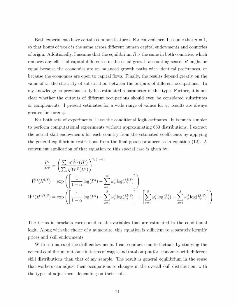
Both experiments have certain common features. For convenience, I assume that σ = 1,

so that hours of work is the same across different human capital endowments and countries

of origin. Additionally, I assume that the equilibrium R is the same in both countries, which

removes any effect of capital differences in the usual growth accounting sense. R might be

equal because the economies are on balanced growth paths with identical preferences, or

because the economies are open to capital flows. Finally, the results depend greatly on the

value of ψ, the elasticity of substitution between the outputs of different occupations. To

my knowledge no previous study has estimated a parameter of this type. Further, it is not

clear whether the outputs of different occupations should even be considered substitutes

or complements. I present estimates for a wide range of values for ψ; results are always

greater for lower ψ.

For both sets of experiments, I use the conditional logit estimates. It is much simpler

to perform computational experiments without approximating 650 distributions. I extract

the actual skill endowments for each country from the estimated coefficients by applying

the general equilibrium restrictions from the final goods producer as in equation (12). A

convenient application of that equation to this special case is given by:

P j

P j′=

(∑i η

iW j(H i)∑i η

iW j′(H i)

)2/(1−ψ)

W j(HUS) = exp

([1

1− αlog(P j) +

S∑s=1

ωjs log(hUSs )

])

W j(H i 6=US) = exp

([1

1− αlog(P j) +

S∑s=1

ωjs log(hUSs )

]+

[S∑s=1

ωjs log(his)−S∑s=1

ωjs log(hUSs )

])

The terms in brackets correspond to the variables that are estimated in the conditional

logit. Along with the choice of a numeraire, this equation is sufficient to separately identify

prices and skill endowments.

With estimates of the skill endowments, I can conduct counterfactuals by studying the

general equilibrium outcome in terms of wages and total output for economies with different

skill distributions than that of my sample. The result is general equilibrium in the sense

that workers can adjust their occupations to changes in the overall skill distribution, with

the types of adjustment depending on their skills.

21

5.1 Effect of Removing All Immigrants

In this section I study the distributional implications of a world in which all immigrants are

removed from the United States. To be clear, I study the changes in the wage distribution

if the United States is composed of only the American-born workers who meet my sample

selection criteria, instead of all workers who meet those criteria. Again, the sample includes

only workers who immigrated after completing their schooling; I view this experiment as

the more interesting one because workers who immigrate later in life are seemingly more

contentious.

Table 2: Changes to the Wage Distribution

ψ

Statistic 0.05 0.1 0.5 1 5 10 20

Min -2.7% -2.6% -2.2% -1.8% -0.8% -0.5% -0.3%

Mediana 1.5% 1.4% 1.2% 1.0% 0.4% 0.2% 0.1%

Max 130.2% 125.7% 98.1% 75.2% 27.7% 15.3% 8.1%a Median of the absolute value of the percentage wage change across all 452

occupations.

Table 2 presents summary statistics for the distributional effects of excluding immi-

grants, for values of the elasticity of substitution ranging from strong complements to

strong substitutes. For each ψ I present the largest wage decrease and increase seen for

any occupation. Removing immigrants would seem to create large benefits for workers in

some occupations against only small losses. These statistics are driven by a variable and

highly skewed distribution of wage changes, as can be easily seen in Figure 3, which plots

the actual distribution of wage changes for ψ = 1. Most workers see only small changes.

This fact is confirmed by the middle row of Table 2, which gives the median of the absolute

value of the wage change; the average occupation sees at most a 1.5% change in their wages.

Another question of interest is which occupations are most affected by these changes.

Table 3 gives information about the three occupations that would see the largest wage

increase and decrease under the experiment. Generally speaking, occupations that would

lose are those that are moderately skill-intensive across all of the categories but physical

skills. They are particularly likely to include occupations that require a high degree of

communication, which fits with the fact that most immigrants are scarce in communications

22

Table 3: Occupations with Largest Wage Changes

Biggest Increase

Rank Occupation %∆a

1 Aerospace Engineers 75.2%

2 Tire Builders 39.0%

3 Pressers, Textile/Garments 35.6%

Biggest Decrease

Rank Occupation %∆a

1 First-Line Supervisor, Housekeeping/Janitorial -1.8%

2 Eligibility Interviewer, Government Programs -1.7%

3 First-Line Supervisor, Landscaping/Lawn -1.6%a Percentage change in wages for ψ = 1. The size of the wage changes but

not the identity of the most affected occupations changes for differentvalues of ψ.

skills. There are two distinct groups of occupations that would see wage increases. The first,

including aerospace engineers and a few related occupations such as physicists, are highly

intensive in cognitive ability and education. Since immigrants from developed countries

possess these cognitive ability in abundance, removing them would raise wages in these

occupations. The second, much larger group is occupations that are relatively unintensive

across all skills except physical skills. The many developing country immigrants have skills

appopriate for these occupations, and removing them tends to raise wages.

The results here are consistent with other general equilibrium results, particularly Ot-

taviano and Peri (2006) and Peri and Sparber (2007). Broadly, these papers find that in a

general equilibrium model with capital adjustment, American and foreign workers are im-

perfect substitutes. They also find that immigration generally has small effects on wages,

with only the least-skilled Americans seeing falling wages. This paper suggests that workers

are imperfect substitutes because of large skill differences. In particular, Mexican immi-

grants (who form a large fraction of the total sample) are physical skill-abundant and scarce

in all other skills relative to Americans. The Americans most likely to see negative wage

effects from immigrants are those working in physical skill-intensive occupations. Finally,

my results on the effects of high-skilled workers receive some support in the recent findings

23

of Borjas (2005). He shows that increases in the number of immigrants entering into U.S.

PhD programs in a particular field are associated with declines in the wages of doctoral

graduates in that field. While these workers would not be included in my sample, I take

these results as evidence that immigrants can depress wages for some specific high-skilled

workers. Further, my results could help explain why immigrants study certain fields, such

as hard sciences and engineering, more than others, such as social sciences. In particular,

one could infer that a lack of communication skills makes more discussion-based subjects

such as psychology and sociology less attractive.10

5.2 Effect of Removing Low-Skilled Immigrants

In progress.

6 Conclusion

This paper has proposed a simple theory of labor markets where workers vary in their

endowment of a vector of skills, and occupations vary in their intensity over the vector of

skills. The key theoretical result is a pseudo-Rybczynski Theorem. Where sufficient data

on human capital endowments are available, the Theorem seems broadly supported. Where

data are not available, the model provides a tractable way to estimate human capital en-

dowments. Implementation to estimate the skills of immigrants from different countries

suggests interesting differences between Americans and immigrants, and between immi-

grants from different countries. Experiments using the general equilibrium model suggest

that American workers see small wage changes as long as they can substitute into a com-

munications or experience and training-intensive occupation, but that they may see large

wage changes otherwise.

This model has abstracted from the skill accumulation decisions of workers by using

an endowment framework. Additionally, it has purposefully taken a long-run view, leaving

many short-run issues unexplored. Principal among these is the transition path of workers’

careers as they respond to immigration and the costs that they pay to switch occupations.

These issues are left for future work.

10See Table 1 of his paper for percentage foreign-born by field.

24

References

Autor, D. H., F. Levy, and R. J. Murnane (2003): “The Skill Content of Recent

Technological Change: An Empirical Exploration,” The Quarterly Journal of Economics,

118(4), 1279–1333.

Borjas, G. J. (1999): “The Economic Analysis of Immigration,” in Handbook of Labor

Economics, ed. by O. Ashenfelter, and D. Card, vol. 3A, pp. 1697–1760. Elsevier Science,

North-Holland Publishers.

(2005): “The Labor-Market Impact of High-Skill Immigration,” The American

Economic Review, 95(2), 56–60.

Gathmann, C., and U. Schonberg (2006): “How General is Specific Human Capital?,”

Working Paper, Hoover Institution.

Heckscher, E. (1949): “The Effect of Foreign Trade on the DIstribution of Income,” in

Readings in the Theory of International Trade, chap. 13, pp. 272–300. Blakiston.

Hensher, D. A., and W. H. Greene (2001): “The Mixed Logit Model: The State of

Practice and Warnings for the Unwary,” Mimeo, New York University.

Lazear, E. P. (2003): “Firm-Specific Human Capital: A Skill-Weights Approach,” NBER

Working Paper No. w9679.

McFadden, D. (1974): “Conditional Logit Analysis of Qualitative Choice Analysis,” in

Frontiers in Econometrics, ed. by P. Zarembka, pp. 105–142. New York: Academic Press.

Occupational Information Network (O*NET) and US Department of

Labor/Employment and Training Administration (USDOL/ETA) (2007):

“Database 12.0,” Available online at http://www.onetcenter.org/overview.html.

Office of Policy and Planning U.S. Immigration and Naturaliza-

tion Service (2003): “Estimates of the unauthorized immigrant popula-

tion residing in the United States: 1990 to 2000,” Available online at

http://www.dhs.gov/xlibrary/assets/statistics/publications/Ill Report 1211.pdf.

Ohlin, B. (1933): Interregional and International Trade. Harvard University Press, Cam-

bridge.

25

Ottaviano, G. I., and G. Peri (2006): “Rethinking the Effects of Immigration on

Wages,” Working Paper.

Peri, G., and C. Sparber (2007): “Task Specialization, Comparative Advantages, and

the Effects of Immigration on Wages,” Working Paper.

Ruggles, S., M. Sobek, T. Alexander, C. A. Fitch, R. Goeken, P. K. Hall,

M. King, and C. Ronnander (2004): “Integrated Public Use Microdata Series: Ver-

sion 3.0 [Machine-readable database],” Minneapolis, MN: Minnesota Population Center

[producer and distributor], http://www.ipums.org.

Spitz-Oener, A. (2006): “Technical Change, Job Tasks, and Rising Educational De-

mands: Looking outside the Wage Structure,” Journal of Labor Economics, 24(2), 235–

270.

Train, K. (2003): Discrete Choice Models with Simulation. Cambridge University Press.

U.S. Department of Labor, Employment, and Training Administration (1991):

“Dictionary of Occupational Titles: Revised Fourth Edition,” Washington DC: 1991.

World Bank (2006): World Development Indicators.

26

A Measures of Skill Intensity

A.1 Information Used

The O*NET database is built on a content model that divides occupational information into

six broad categories: worker characteristics, worker requirements, experience requirements,

occupation-specific information, workforce characteristics, and occupational requirements.

Within each of these six broad categories information is organized in a hierarchical format

similar to the 1-digit, 2-digit, 3-digit format of industry and trade data. For instance, item

1.A.1.a.1 is a 5-digit characteristic of occupations, going from general to specific: Worker

Characteristics.Ability.Cognitive Abilities.Verbal Abilities.Oral Comprehension. Through-

out, I use the most disaggregated data possible, which can be 3 to 6-digit information.

Data are provided for each category and occupation, and is typically normalized to a

0-7 scale. O*NET provides anchors that represent typical characteristics associated with

particular scores. For example, Oral Comprehension is computed on a scale of 0-7. The

anchors given are that a score of 2 is equivalent to ability to understand a television com-

mercial; a score of 4 is equivalent to ability to understand a coach’s oral instructions for a

sport; and a score of 6 is equivalent to ability to understand a lecture on advanced physics.

Scores for each occupation-attribute are gathered either from the average score given by

occupational analysts or the average score given by survey responses from incumbent work-

ers. For instance, all oral comprehension scores are the average rating of eight analysts,

while the mathematics skills score for chief executives is the average of 23 survey responses

by actual chief executives.

From the 250+ most disaggregated categories I select those that correspond closely to

one of the five skills. I also focus on information that is relatively unique to a specific skill.

The reported level anchors are helpful here. For example, I exclude oral comprehension

ability because it is not clear from the anchors provided whether it measures a cognitive

ability, a communication skill, or a mixture. I give a broad description of the information

used in each skill here; the specific measures are provided in Tables (5) - (9). Education and

knowledge consists of subject knowledge requirements for subjects only learned in school and

a measure of education required for the occupation. Training and experience is a mixture

of measures of different types of training required for the job, plus a measure of actual job-

specific experience that workers report having. Cognitive abilities are measured using the

cognitive abilities category, minus those abilities which have speech components. Physical

27

skills are measured using information from the physical abilities category. Language and

communication is measured using information on how likely workers were to interact with

others, and the frequency of different methods of communication.

I use principal component analysis to aggregate the different measures into a single skill

intensity for each dimension. I keep only the first component, which accounts for 36-82% of

the total variation of the variables. I denote with a * variables that have at least one-third

of their variation accounted for by the principal component, indicating that they are well-

represented in the resulting skill intensity measure. This criteria produces similar results

to the common technique of identifying variables that have factor loadings exceeding a

threshold of 35 or 40. For each of the five dimensions, I also identify the three occupations

that score as the most skill-intensive, and the three that score as the least skill-intensive.

No occupation is repeated on this list, and more generally no cross-intensity correlation

exceeds 0.60, implying sufficient variation to identify the skill components separately.

28

Table 4: Estimated Human Capital, Conditional Logit

Country Obs Communication Exp/Train Cognitive Physical Education

United States 6306216 0 0 0 0 0

Puerto Rico 16391 -2.156* -1.036* -0.4876* 0.5372** 0.326**

Canada 11182 -0.5482* -0.0790 2.524** -1.065* 0.7379**

Bermuda 162 1.037* 0.8599 -1.995* -0.2743 -0.3250

Cape Verde 517 -4.412* -1.202* -0.8577* 0.0331 0.1774

Mexico 209687 -2.7* -0.6486* -2.085* 2.099** -0.2327*

Belize 696 -0.6841* -2.139* 1.342** 0.8456** 0.3584

Costa Rica 1439 -2.066* -0.6773* -1.528* 0.3238** 0.653**

El Salvador 20822 -3.225* -1.214* -1.732* 1.11** 0.4222**

Guatemala 12225 -3.178* -1.098* -1.575* 1.282** 0.2586**

Honduras 6961 -2.658* -1.085* -1.922* 1.469** 0.5583**

Nicaragua 4279 -1.928* -0.9486* -1.335* 0.4613** 0.0917

Panama 1827 -0.7001* -1.793* 0.7754** -0.4141* 0.2455*

Cuba 13381 -1.083* -0.4592* -0.7238* 0.7565** -0.7824*

Dominican Republic 12739 -2.621* -2.399* 0.3483** 0.7928** -0.1772*

Haiti 8911 -2.438* -4.394* 1.467** 1.536** 1.696**

Jamaica 10350 -0.9417* -3.064* 2.056** 1.346** 1.294**

Antigua-Barbuda 342 -0.8664* -2.082* 0.7793* 0.3582 1.086**

Bahamas 322 -0.0878 -1.894* 0.1889 0.4099 1.051**

Barbados 949 -1.33* -2.53* 0.8787** 0.7364** 1.797**

Dominica 341 -2.328* -2.229* 1.375** 0.6719** 1.442**

Grenada 553 -0.9979* -2.882* 1.789** 1.138** 1.879**

St. Kitts-Nevis 221 -1.167* -2.336* 1.916** 0.5283 0.4396

St. Lucia 275 -0.7013* -1.958* 0.8112 1.277** 0.5667

St. Vincent 376 -1.217* -2.775* 1.505** 1.292** 1.313**

Trinidad and Tobago 3635 -0.7954* -2.308* 1.872** 0.6467** 0.6725**

Argentina 2410 -1.166* 0.2241 0.6306** -0.628* 0.5365**

Bolivia 1091 -1.966* -0.6501* -1.172* -0.3677* 0.83**

Brazil 4891 -2.579* -0.9117* -0.639* -0.7596* 1.284**

Chile 1569 -1.545* -0.6005* -0.0007 -0.2369* 0.967**

Colombia 10741 -2.47* -1.024* -0.196* -0.1805* 0.2299**

Ecuador 6161 -2.635* -1.269* -0.2488* 0.7079** -0.6927*

Guyana 4073 -0.6563* -2.553* 1.968** 0.6905** 0.1202

Paraguay 243 -2.773* 0.1894 -2.269* -0.8393* 1.995**

Peru 6292 -2.085* -0.9174* -0.5211* -0.1778* 0.335**

Uruguay 523 -1.01* 0.0932 -0.4601 0.0473 -0.3719

Continued on Next Page

29



Venezuela 1804 -0.7859* -0.5952* 1.124** -0.8221* 0.0101

Denmark 523 -0.1445 0.7328** 2.099** -1.205* 0.1608

Finland 384 -0.9161* -0.6332* 3.859** -0.7376* 0.4565

Norway 408 -0.0703 0.6008 2.364** -1.155* 0.46*

Sweden 879 -0.7039* -0.815* 3.779** -1.05* 0.1120

United Kingdom 11460 -0.2699* 0.0904 2.727** -1.47* -0.0719

Ireland 2689 0.1932 0.6877** 0.5769** 0.1247 -0.0322

Belgium 384 -0.6955* 0.1402 2.634** -1.733* 0.3572

France 2335 -0.8854* 0.1060 2.467** -1.581* 0.3825**

Netherlands 1172 -0.8123* 0.8162** 2.489** -1.221* 0.4263**

Switzerland 758 -1.387* 0.8554** 3.439** -1.746* 0.2414

Albania 758 -2.332* -1.34* -0.5592* 0.1947 -0.4380

Greece 2406 -0.6087* -1.18* 1.767** 0.8894** -0.932*

Macedonia 397 -1.66* -1.142* 0.0983 1.292** -1.436*

Italy 5066 -2.216* 0.7682** 0.3532** -0.1216* -0.3478*

Portugal 3388 -3.148* 0.8302** -1.073* 0.6998** -0.5384*

Azores 398 -3.236* 0.2143 -1.244* 1.688** -0.7997*

Spain 1548 -1.445* 0.7819** -0.2840 -0.7992* 1.159**

Austria 502 -1.576* 0.8571** 2.087** -1.616* 0.4274*

Bulgaria 758 -2.103* -1.113* 2.079** -0.5779* 0.535**

Czechoslovakia 526 -1.718* 0.4632 0.7211* -0.3019 0.1659

Slovakia 285 -1.244* 0.4239 -0.0803 -0.1273 -0.1882

Czech Republic 432 -1.568* -0.4930 0.917** 0.0965 0.4100

Germany 9463 -0.6954* -0.4642* 1.486** -0.9072* 0.0040

Hungary 1045 -1.706* 0.8635** 1.481** -0.4215* -0.1918

Poland 8518 -2.537* 0.8643** -0.0261 0.0231 -0.1628*

Romania 2493 -2.414* 0.0090 2.537** -0.4085* 0.1401

Yugoslavia 1377 -2.098* 0.0772 -0.2141 -0.1496 -0.4371*

Croatia 711 -2.07* 1.314** -0.1632 0.0841 -0.3763

Serbia 193 -1.593* 0.2211 -0.9802* -0.1394 -0.0377

Bosnia 2093 -3.456* -0.4476* -0.1799 0.2108* -0.7051*

Kosovo 175 -2.44* -1.2* -1.786* -0.0234 -0.1425

Latvia 228 -2.215* 0.0323 3.025** -1.575* 0.0846

Lithuania 286 -2.125* -0.7425* 3.457** -0.3364 0.1614

Belarus 657 -1.658* -1.159* 4.013** 0.1042 -1.137*

Moldavia 364 -1.375* -0.3431 2.156** 0.1374 -0.5933*

Ukraine 4385 -2.206* -0.66* 2.845** -0.3553* -0.5501*


30



Armenia 924 -0.1062 -1.512* 1.481** 1.103** -0.6179*

Azerbaijan 256 -1.718* -0.9584* 2.158** -0.3665 -0.1337

Georgia 180 -1.806* -2.054* 2.654** 0.2327 1.39**

Uzbekistan 369 -2.428* -1.668* 3.246** -0.4395* 0.3546

China 19752 -4.261* -1.878* 3.926** -1.506* 0.5342**

Hong Kong 2731 -1.593* -1.437* 2.583** -1.322* -0.9025*

Taiwan 5724 -1.082* -0.3637* 3.99** -1.896* -0.5103*

Japan 6320 -0.8975* -0.7577* 2.712** -1.565* 0.2191**

South Korea 2331 -1.521* -1.298* 1.764** -0.5253* -0.2838*

Cambodia 2266 -4.24* -1.394* 2.307** -0.0330 -1.937*

Indonesia 1065 -1.275* -1.962* 2.957** -0.62* -0.0089

Laos 3159 -5.343* -0.536* 1.585** 0.3849** -2.033*

Malaysia 901 -1.56* -1.828* 2.837** -1.184* 0.0008

Philippines 30424 -2.155* -2.671* 2.967** -0.239* 1.01**

Singapore 369 -0.8303* -1.611* 4.188** -1.71* -0.1589

Thailand 2410 -2.815* -2.675* 2.692** -0.3728* 0.4962**

Vietnam 19637 -4.632* -0.7654* 2.691** -0.4626* -1.953*

Afghanistan 690 0.0394 -3.464* 3.673** 1.056** -1.381*

India 19615 -3.205* -1.211* 4.874** -1.815* 0.3292**

Bangladesh 1684 -0.6902* -4.44* 3.717** 0.5029** -0.5989*

Myanmar 768 -2.878* -0.9267* 3.02** -0.4234* -0.3183

Pakistan 3832 -0.3988* -3.552* 4.661** 0.7172** -0.9508*

Sri Lanka 619 -1.655* -1.952* 3.961** -1.125* 1.038**

Iran 4561 0.0996 -0.7923* 2.58** -0.4186* -0.4117*

Nepal 254 -2.449* -3.385* 2.745** -1.121* 0.8992**

Cyprus 159 -1.467* -0.4963 2.299** -0.3231 -0.4363

Iraq 1536 -1.434* -1.114* 1.694** 0.552** -1.094*

Israel/Palestine 1913 -0.0085 -0.0898 2.066** -0.8924* -0.0980

Jordan 692 1.191** -2.825* 3.145** 1.197** -1.452*

Kuwait 180 0.2753 -3.23* 4.288** 0.5178 0.2436

Lebanon 1595 0.0907 -0.6351* 1.961** -0.1398 -0.7541*

Saudi Arabia 162 -1.313* -0.2761 1.988** -0.3540 0.7918*

Syria 875 0.1504 -1.218* 1.96** 0.633** -1.024*

Turkey 1352 -1.139* -0.9249* 2.295** -0.4201* -0.1264

Yemen 295 -0.7205* -3.46* 2.129** 0.8011** -2.131*

Algeria 241 -0.8142* -2.733* 3.713** -0.4045 -0.1858

Egypt 2214 -0.6016* -1.961* 3.492** -0.2458* 0.319**


31



Morocco 809 0.1523 -2.655* 1.843** 0.2016 -0.5905*

Sudan 351 -2.79* -3.383* 2.736** 0.1627 0.4814

Ghana 1627 -1.611* -4.443* 3.64** 0.8606** 1.412**

Liberia 786 -1.234* -4.812* 3.53** 0.8885** 1.906**

Nigeria 2831 -0.4906* -4.449* 4.735** 0.7132** 1.806**

Senegal 242 -0.3649 -2.77* 1.343** 0.4169 -0.9041*

Sierra Leone 491 -0.5825* -5.578* 4.234** 1.246** 1.805**

Ethiopia 1508 -0.5532* -5.772* 3.57** 1.088** -0.4281*

Kenya 814 -1.312* -3.601* 3.784** -0.7993* 1.195**

Somalia 512 -2.643* -4.204* 1.914** 0.9856** -0.5781

Tanzania 244 -1.625* -1.357* 3.252** -1.143* 0.8143**

Uganda 272 -1.553* -2.425* 4.255** -0.4210 0.8034**

Zimbabwe 238 -1.17* -0.85* 3.305** -0.9891* 0.7377*

Eritrea 374 -1.726* -4.883* 3.119** 0.9339** 0.1485

Cameroon 247 -0.5907 -4.484* 4.758** 0.2425 1.114**

South Africa 1318 -0.2356 0.2704 2.839** -1.985* 0.5765**

Australia 1253 -0.7372* -0.3824* 2.983** -1.575* 0.8133**

New Zealand 560 -0.4286 0.6629* 2.254** -0.8864* 0.5254**

Fiji 661 -2.002* -2.036* 1.408** 0.3814* -0.1194

Tonga 307 -1.43* -1.577* -0.2214 1.863** 0.3555

Western Samoa 286 -0.2369 -0.6007 -1.416* 0.7655** -1.74*

Note: All values are estimates of the difference in log-skills between that country and the

United States. A single * denotes significance at the 95% level, and ** denotes significance

at the 99% confidence level. Obs is the number of observations in the 5% sample of the

2000 U.S. Census meeting the sample criteria for that country.

32

Table 5: Dimensions of Human Capital: Education and Knowledge

Measurea Intensity Rankingb

Knowledge Category Most Intensive

Engineering and Technology 1. Physicians and Surgeons

Design 2. Miscellaneous Social Scientists

Mathematics 3. Dieticians and Nutritionists

Physics

Chemistry Least Intensive

Biology* 1. Food and Tobacco Machine Operator/Tender

Psychology* 2. Taxi Driver and Chauffeur

Sociology* 3. Desktop Publishers

Geography

Medicine and Dentistry*

Therapy and Counseling*

Foreign Language*

Fine Arts

History and Archaelogy*

Philosophy and Theology*

Law and Government*

Other Category

Required Education Level*a Name of measure in O*NET system. An asterisk indicates that the first principal

component captures at least 1/3 of the variation in the measure.b Three occupations that score highest and lowest for skill intensity.

33

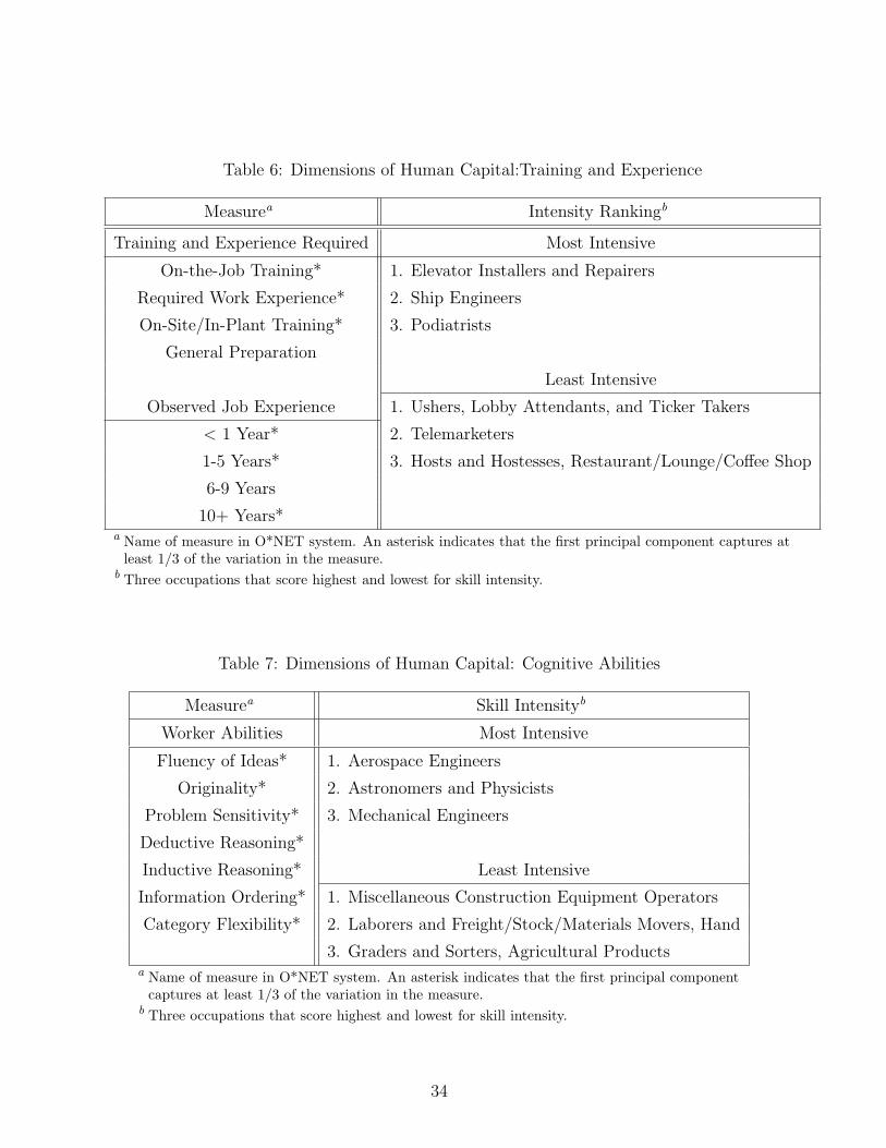
Table 6: Dimensions of Human Capital:Training and Experience


Training and Experience Required Most Intensive

On-the-Job Training* 1. Elevator Installers and Repairers

Required Work Experience* 2. Ship Engineers

On-Site/In-Plant Training* 3. Podiatrists

General Preparation

Least Intensive

Observed Job Experience 1. Ushers, Lobby Attendants, and Ticker Takers

< 1 Year* 2. Telemarketers

1-5 Years* 3. Hosts and Hostesses, Restaurant/Lounge/Coffee Shop

6-9 Years

10+ Years*a Name of measure in O*NET system. An asterisk indicates that the first principal component captures at

least 1/3 of the variation in the measure.b Three occupations that score highest and lowest for skill intensity.

Table 7: Dimensions of Human Capital: Cognitive Abilities

Measurea Skill Intensityb

Worker Abilities Most Intensive

Fluency of Ideas* 1. Aerospace Engineers

Originality* 2. Astronomers and Physicists

Problem Sensitivity* 3. Mechanical Engineers

Deductive Reasoning*

Inductive Reasoning* Least Intensive

Information Ordering* 1. Miscellaneous Construction Equipment Operators

Category Flexibility* 2. Laborers and Freight/Stock/Materials Movers, Hand

3. Graders and Sorters, Agricultural Productsa Name of measure in O*NET system. An asterisk indicates that the first principal component

captures at least 1/3 of the variation in the measure.b Three occupations that score highest and lowest for skill intensity.

34

Table 8: Dimensions of Human Capital: Physical Abilities


Ability Most Intensive

Arm-Hand Steadiness* 1. Fire Fighters

Manual Dexterity* 2. Electricians

Finger Dexterity* 3. Emergency Medical Technicians and Paramedics

Control Precision*

Multilimb Coordination* Least Intensive

Response Orientation* 1. Public Relations Specialist

Rate Control* 2. Actuaries

Reaction Time* 3. Proofreaders and Copy Markers

Wrist-Finger Speed*

Speed of Limb Movement*

Static Strength Ability*

Explosive Strength

Dynamic Strength*

Trunk Strength*

Stamina*

Extent Flexibility*

Dynamic Flexibility

Gross Body Coordination*

Gross Body Equilibrium*

Near Vision

Far Vision

Visual Color Discrimination*

Night Vision*

Peripheral Vision*

Depth Perception*

Glare Sensitivity*

Hearing Sensitivity*

Auditory Attention*a Name of measure in O*NET system. An asterisk indicates that the first principal component

captures at least 1/3 of the variation in the measure.b Three occupations that score highest and lowest for skill intensity.

35

Table 9: Dimensions of Human Capital: Language and Communication


Frequency of Communication by Method Most Intensive

Public Speaking* 1. Gaming Managers

Telephone* 2. Postmasters and Mail Superintendents

Letters and Memos* 3. Urban and Regional Planners

Face-to-Face Discussions*

Least Intensive

Frequency of Communication by Type 1. Pressers, Textile, Garment, and Related Materials

Contact with Others* 2. Tire Builders

Work with Group or Team* 3. Shoe Machine Operators and Tenders

Deal with External Customers*a Name of measure in O*NET system. An asterisk indicates that the first principal component captures at least

1/3 of the variation in the measure.b Three occupations that score highest and lowest for skill intensity.

36

-6-4-20246

010

000

2000

030

000

4000

0

PPP

GD

P p.

c.

Log Skill-Ratio

Com

mun

icat

ion

Cog

nitiv

eE

duca

tion

Line

ar (C

omm

unic

atio

n)Li

near

(Cog

nitiv

e)Li

near

(Edu

catio

n)

Figure 1: Skills - GDP Relationship37

-6-4-20246

010

000

2000

030

000

4000

0

PPP

GD

P p.

c.

Log Skill-Ratio

Exp

erie

nce

Phy

sica

lLi

near

(Exp

erie

nce)

Line

ar (P

hysi

cal)

Figure 2: Skills - GDP Relationship38

0

40

80

120

160

95%

105%

115%

125%

135%

145%

155%

165%

175%

% of Previous Wage

Num

ber o

f Occ

upat

ions

Figure 3: Distribution of Changes to Wages

39

The Occupations and Human Capital of U.S. Immigrants · employment across Census-level occupations...

Documents

Transcript of The Occupations and Human Capital of U.S. Immigrants · employment across Census-level occupations...