
The Nonstochastic Multiarmed Bandit Problem
30
THE NONSTOCHASTIC MULTIARMED BANDIT PROBLEM ∗ PETER AUER † , NICOL ` O CESA-BIANCHI ‡ , YOAV FREUND § , AND ROBERT E. SCHAPIRE ¶ SIAM J. COMPUT. c 2002 Society for Industrial and Applied Mathematics Vol. 32, No. 1, pp. 48–77 Abstract. In the multiarmed bandit problem, a gambler must decide which arm of K non- identical slot machines to play in a sequence of trials so as to maximize his reward. This classical problem has received much attention because of the simple model it provides of the trade-off between exploration (trying out each arm to find the best one) and exploitation (playing the arm believed to give the best payoff). Past solutions for the bandit problem have almost always relied on assumptions about the statistics of the slot machines. In this work, we make no statistical assumptions whatsoever about the nature of the process generating the payoffs of the slot machines. We give a solution to the bandit problem in which an adversary, rather than a well-behaved stochastic process, has complete control over the payoffs. In a sequence of T plays, we prove that the per-round payoff of our algorithm approaches that of the best arm at the rate O(T −1/2 ). We show by a matching lower bound that this is the best possible. We also prove that our algorithm approaches the per-round payoff of any set of strategies at a similar rate: if the best strategy is chosen from a pool of N strategies, then our algorithm approaches the per-round payoff of the strategy at the rate O((log N ) 1/2 T −1/2 ). Finally, we apply our results to the problem of playing an unknown repeated matrix game. We show that our algorithm approaches the minimax payoff of the unknown game at the rate O(T −1/2 ). Key words. adversarial bandit problem, unknown matrix games AMS subject classifications. 68Q32, 68T05, 91A20 PII. S0097539701398375 1. Introduction. In the multiarmed bandit problem, originally proposed by Robbins [17], a gambler must choose which of K slot machines to play. At each time step, he pulls the arm of one of the machines and receives a reward or payoff (possibly zero or negative). The gambler’s purpose is to maximize his return, i.e., the sum of the rewards he receives over a sequence of pulls. In this model, each arm is assumed to deliver rewards that are independently drawn from a fixed and unknown distribution. As reward distributions differ from arm to arm, the goal is to find the arm with the highest expected payoff as early as possible and then to keep gambling using that best arm. The problem is a paradigmatic example of the trade-off between exploration and exploitation. On the one hand, if the gambler plays exclusively on the machine that he thinks is best (“exploitation”), he may fail to discover that one of the other arms actually has a higher expected payoff. On the other hand, if he spends too much time ∗ Received by the editors November 18, 2001; accepted for publication (in revised form) July 7, 2002; published electronically November 19, 2002. An early extended abstract of this paper appeared in Proceedings of the 36th Annual Symposium on Foundations of Computer Science, 1995, IEEE Computer Society, pp. 322–331. http://www.siam.org/journals/sicomp/32-1/39837.html † Institute for Theoretical Computer Science, Graz University of Technology, A-8010 Graz, Austria ([email protected]). This author gratefully acknowledges the support of ESPRIT Working Group EP 27150, Neural and Computational Learning II (NeuroCOLT II). ‡ Department of Information Technology, University of Milan, I-26013 Crema, Italy (cesa-bianchi@ dti.unimi.it). This author gratefully acknowledges the support of ESPRIT Working Group EP 27150, Neural and Computational Learning II (NeuroCOLT II). § Banter Inc. and Hebrew University, Jerusalem, Israel ([email protected]). ¶ AT&T Labs – Research, Shannon Laboratory, Florham Park, NJ 07932-0971 (schapire@research. att.com). 48 Downloaded 11/11/14 to 131.193.178.178. Redistribution subject to SIAM license or copyright; see http://www.siam.org/journals/ojsa.php
Transcript of The Nonstochastic Multiarmed Bandit Problem
THE NONSTOCHASTIC MULTIARMED BANDIT PROBLEM∗
PETER AUER† , NICOLO CESA-BIANCHI‡ , YOAV FREUND§ , AND
ROBERT E. SCHAPIRE¶
SIAM J. COMPUT. c© 2002 Society for Industrial and Applied MathematicsVol. 32, No. 1, pp. 48–77
Abstract. In the multiarmed bandit problem, a gambler must decide which arm of K non-identical slot machines to play in a sequence of trials so as to maximize his reward. This classicalproblem has received much attention because of the simple model it provides of the trade-off betweenexploration (trying out each arm to find the best one) and exploitation (playing the arm believed togive the best payoff). Past solutions for the bandit problem have almost always relied on assumptionsabout the statistics of the slot machines.
In this work, we make no statistical assumptions whatsoever about the nature of the processgenerating the payoffs of the slot machines. We give a solution to the bandit problem in which anadversary, rather than a well-behaved stochastic process, has complete control over the payoffs. Ina sequence of T plays, we prove that the per-round payoff of our algorithm approaches that of thebest arm at the rate O(T−1/2). We show by a matching lower bound that this is the best possible.
We also prove that our algorithm approaches the per-round payoff of any set of strategies at asimilar rate: if the best strategy is chosen from a pool of N strategies, then our algorithm approachesthe per-round payoff of the strategy at the rate O((logN)1/2T−1/2). Finally, we apply our results tothe problem of playing an unknown repeated matrix game. We show that our algorithm approachesthe minimax payoff of the unknown game at the rate O(T−1/2).
Key words. adversarial bandit problem, unknown matrix games
AMS subject classifications. 68Q32, 68T05, 91A20
PII. S0097539701398375
1. Introduction. In the multiarmed bandit problem, originally proposed byRobbins [17], a gambler must choose which of K slot machines to play. At each timestep, he pulls the arm of one of the machines and receives a reward or payoff (possiblyzero or negative). The gambler’s purpose is to maximize his return, i.e., the sum ofthe rewards he receives over a sequence of pulls. In this model, each arm is assumed todeliver rewards that are independently drawn from a fixed and unknown distribution.As reward distributions differ from arm to arm, the goal is to find the arm with thehighest expected payoff as early as possible and then to keep gambling using that bestarm.
The problem is a paradigmatic example of the trade-off between exploration andexploitation. On the one hand, if the gambler plays exclusively on the machine thathe thinks is best (“exploitation”), he may fail to discover that one of the other armsactually has a higher expected payoff. On the other hand, if he spends too much time
∗Received by the editors November 18, 2001; accepted for publication (in revised form) July 7,2002; published electronically November 19, 2002. An early extended abstract of this paper appearedin Proceedings of the 36th Annual Symposium on Foundations of Computer Science, 1995, IEEEComputer Society, pp. 322–331.
http://www.siam.org/journals/sicomp/32-1/39837.html†Institute for Theoretical Computer Science, Graz University of Technology, A-8010 Graz, Austria
([email protected]). This author gratefully acknowledges the support of ESPRIT WorkingGroup EP 27150, Neural and Computational Learning II (NeuroCOLT II).
‡Department of Information Technology, University of Milan, I-26013 Crema, Italy ([email protected]). This author gratefully acknowledges the support of ESPRIT Working Group EP 27150,Neural and Computational Learning II (NeuroCOLT II).
§Banter Inc. and Hebrew University, Jerusalem, Israel ([email protected]).¶AT&T Labs – Research, Shannon Laboratory, Florham Park, NJ 07932-0971 (schapire@research.
att.com).
48
Dow
nloa
ded
11/1
1/14
to 1
31.1
93.1
78.1
78. R
edis
trib
utio
n su
bjec
t to
SIA
M li
cens
e or
cop
yrig
ht; s
ee h
ttp://
ww
w.s
iam
.org
/jour
nals
/ojs
a.ph
p
THE NONSTOCHASTIC MULTIARMED BANDIT PROBLEM 49
trying out all the machines and gathering statistics (“exploration”), he may fail toplay the best arm often enough to get a high return.
The gambler’s performance is typically measured in terms of “regret.” This is thedifference between the expected return of the optimal strategy (pulling consistentlythe best arm) and the gambler’s expected return. Lai and Robbins proved thatthe gambler’s regret over T pulls can be made, for T → ∞, as small as O(lnT ).Furthermore, they prove that this bound is optimal in the following sense: there isno strategy for the gambler with a better asymptotic performance.
Though this formulation of the bandit problem allows an elegant statistical treat-ment of the exploration-exploitation trade-off, it may not be adequate to model certainenvironments. As a motivating example, consider the task of repeatedly choosing aroute for transmitting packets between two points in a communication network. Tocast this scenario within the bandit problem, suppose there is a only a fixed numberof possible routes and the transmission cost is reported back to the sender. Now, itis likely that the costs associated with each route cannot be modeled by a stationarydistribution, so a more sophisticated set of statistical assumptions would be required.In general, it may be difficult or impossible to determine the right statistical assump-tions for a given domain, and some domains may exhibit dependencies to an extentthat no such assumptions are appropriate.
To provide a framework where one could model scenarios like the one sketchedabove, we present the adversarial bandit problem, a variant of the bandit problemin which no statistical assumptions are made about the generation of rewards. Weassume only that each slot machine is initially assigned an arbitrary and unknownsequence of rewards, one for each time step, chosen from a bounded real interval.Each time the gambler pulls the arm of a slot machine, he receives the correspondingreward from the sequence assigned to that slot machine. To measure the gambler’sperformance in this setting we replace the notion of (statistical) regret with thatof worst-case regret. Given any sequence (j1, . . . , jT ) of pulls, where T > 0 is anarbitrary time horizon and each jt is the index of an arm, the worst-case regret ofa gambler for this sequence of pulls is the difference between the return the gamblerwould have had by pulling arms j1, . . . , jT and the actual gambler’s return, whereboth returns are determined by the initial assignment of rewards. It is easy to seethat, in this model, the gambler cannot keep his regret small (say, sublinear in T )for all sequences of pulls and with respect to the worst-case assignment of rewards tothe arms. Thus, to make the problem feasible, we allow the regret to depend on the“hardness” of the sequence of pulls for which it is measured, where the hardness of asequence is roughly the number of times one has to change the slot machine currentlybeing played in order to pull the arms in the order given by the sequence. This trickallows us to effectively control the worst-case regret simultaneously for all sequencesof pulls, even though (as one should expect) our regret bounds become trivial whenthe hardness of the sequence (j1, . . . , jT ) we compete against gets too close to T .
As a remark, note that a deterministic bandit problem was also considered byGittins [9] and Ishikida and Varaiya [13]. However, their version of the bandit problemis very different from ours: they assume that the player can compute ahead of timeexactly what payoffs will be received from each arm, and their problem is thus one ofoptimization, rather than exploration and exploitation.
Our most general result is a very efficient, randomized player algorithm whose ex-pected regret for any sequence of pulls is1 O(S
√KT ln(KT )), where S is the hardness
1Though in this introduction we use the compact asymptotic notation, our bounds are provenfor each finite T and almost always with explicit constants.
Dow
nloa
ded
11/1
1/14
to 1
31.1
93.1
78.1
78. R
edis
trib
utio
n su
bjec
t to
SIA
M li
cens
e or
cop
yrig
ht; s
ee h
ttp://
ww
w.s
iam
.org
/jour
nals
/ojs
a.ph
p
50 AUER, CESA-BIANCHI, FREUND, AND SCHAPIRE
of the sequence (see Theorem 8.1 and Corollaries 8.2, 8.4). Note that this bound holdssimultaneously for all sequences of pulls, for any assignments of rewards to the arms,and uniformly over the time horizon T . If the gambler is willing to impose an upperbound S on the hardness of the sequences of pulls for which he wants to measurehis regret, an improved bound O(
√SKT ln(KT )) on the expected regret for these
sequences can be proven (see Corollaries 8.3 and 8.5).With the purpose of establishing connections with certain results in game theory,
we also look at a special case of the worst-case regret, which we call “weak regret.”Given a time horizon T , call “best arm” the arm that has the highest return (sum ofassigned rewards) up to time T with respect to the initial assignment of rewards. Thegambler’s weak regret is the difference between the return of this best arm and theactual gambler’s return. In the paper we introduce a randomized player algorithm,tailored to this notion of regret, whose expected weak regret is O(
√KGmax lnK),
where Gmax is the return of the best arm—see Theorem 4.1 in section 4. As before,this bound holds for any assignments of rewards to the arms and uniformly over thechoice of the time horizon T . Using a more complex player algorithm, we also provethat the weak regret is O(
√KT ln(KT/δ)) with probability at least 1 − δ over the
algorithm’s randomization, for any fixed δ > 0; see Theorems 6.3 and 6.4 in section 6.This also implies that, asymptotically for T → ∞ and K constant, the weak regret isO(√
T (lnT )1+ε) with probability 1 for any fixed ε > 0; see Corollary 6.5.Our worst-case bounds may appear weaker than the bounds proved using statis-
tical assumptions, such as those shown by Lai and Robbins [14] of the form O(lnT ).However, when comparing our results to those in the statistics literature, it is im-portant to point out an important difference in the asymptotic quantification. In thework of Lai and Robbins, the assumption is that the distribution of rewards that isassociated with each arm is fixed as the total number of iterations T increases toinfinity. In contrast, our bounds hold for any finite T , and, by the generality of ourmodel, these bounds are applicable when the payoffs are randomly (or adversarially)chosen in a manner that does depend on T . It is this quantification order, and notthe adversarial nature of our framework, which is the cause for the apparent gap. Weprove this point in Theorem 5.1, where we show that, for any player algorithm for theK-armed bandit problem and for any T , there exists a set of K reward distributionssuch that the expected weak regret of the algorithm when playing on these arms forT time steps is Ω(
√KT ).
So far we have considered notions of regret that compare the return of the gamblerto the return of a sequence of pulls or to the return of the best arm. A furthernotion of regret which we explore is the regret for the best strategy in a given setof strategies that are available to the gambler. The notion of “strategy” generalizesthat of “sequence of pulls”: at each time step a strategy gives a recommendation, inthe form of a probability distribution over the K arms, as to which arm to play next.Given an assignment of rewards to the arms and a set of N strategies for the gambler,call “best strategy” the strategy that yields the highest return with respect to thisassignment. Then the regret for the best strategy is the difference between the returnof this best strategy and the actual gambler’s return. Using a randomized playerthat combines the choices of the N strategies (in the same vein as the algorithms for“prediction with expert advice” from [3]), we show that the expected regret for thebest strategy is O(
√KT lnN)—see Theorem 7.1. Note that the dependence on the
number of strategies is only logarithmic, and therefore the bound is quite reasonableeven when the player is combining a very large number of strategies.
The adversarial bandit problem is closely related to the problem of learning to
Dow
nloa
ded
11/1
1/14
to 1
31.1
93.1
78.1
78. R
edis
trib
utio
n su
bjec
t to
SIA
M li
cens
e or
cop
yrig
ht; s
ee h
ttp://
ww
w.s
iam
.org
/jour
nals
/ojs
a.ph
p
THE NONSTOCHASTIC MULTIARMED BANDIT PROBLEM 51
play an unknown N -person finite game, where the same game is played repeatedly byN players. A desirable property for a player is Hannan-consistency, which is similarto saying (in our bandit framework) that the weak regret per time step of the playerconverges to 0 with probability 1. Examples of Hannan-consistent player strategieshave been provided by several authors in the past (see [5] for a survey of these results).By applying (slight extensions of) Theorems 6.3 and 6.4, we can provide an example ofa simple Hannan-consistent player whose convergence rate is optimal up to logarithmicfactors.
Our player algorithms are based in part on an algorithm presented by Freund andSchapire [6, 7], which in turn is a variant of Littlestone and Warmuth’s [15] weightedmajority algorithm and Vovk’s [18] aggregating strategies. In the setting analyzed byFreund and Schapire, the player scores on each pull the reward of the chosen arm butgains access to the rewards associated with all of the arms (not just the one that waschosen).
2. Notation and terminology. An adversarial bandit problem is specified bythe number K of possible actions, where each action is denoted by an integer 1 ≤i ≤ K, and by an assignment of rewards, i.e., an infinite sequence x(1),x(2), . . . ofvectors x(t) = (x1(t), . . . , xK(t)), where xi(t) ∈ [0, 1] denotes the reward obtained ifaction i is chosen at time step (also called “trial”) t. (Even though throughout thepaper we will assume that all rewards belong to the [0, 1] interval, the generalizationof our results to rewards in [a, b] for arbitrary a < b is straightforward.) We assumethat the player knows the number K of actions. Furthermore, after each trial t, weassume the player knows only the rewards xi1(1), . . . , xit(t) of the previously chosenactions i1, . . . , it. In this respect, we can view the player algorithm as a sequenceI1, I2, . . . , where each It is a mapping from the set (1, . . . ,K × [0, 1])t−1 of actionindices and previous rewards to the set of action indices.
For any reward assignment and for any T > 0, let
GA(T )def=
T∑t=1
xit(t)
be the return at time horizon T of algorithm A choosing actions i1, i2, . . . . In whatfollows, we will write GA instead of GA(T ) whenever the value of T is clear from thecontext.
Our measure of performance for a player algorithm is the worst-case regret, and inthis paper we explore variants of the notion of regret. Given any time horizon T > 0and any sequence of actions (j1, . . . , jT ), the (worst-case) regret of algorithm A for(j1, . . . , jT ) is the difference
G(j1,...,jT ) −GA(T ),(1)
where
G(j1,...,jT )def=
T∑t=1
xjt(t)
is the return, at time horizon T , obtained by choosing actions j1, . . . , jT . Hence, theregret (1) measures how much the player lost (or gained, depending on the sign of thedifference) by following strategy A instead of choosing actions j1, . . . , jT . A special
Dow
nloa
ded
11/1
1/14
to 1
31.1
93.1
78.1
78. R
edis
trib
utio
n su
bjec
t to
SIA
M li
cens
e or
cop
yrig
ht; s
ee h
ttp://
ww
w.s
iam
.org
/jour
nals
/ojs
a.ph
p
52 AUER, CESA-BIANCHI, FREUND, AND SCHAPIRE
case of this is the regret of A for the best single action (which we will call weak regretfor short), defined by
Gmax(T )−GA(T ),
where
Gmax(T )def= max
j
T∑t=1
xj(t)
is the return of the single globally best action at time horizon T . As before, we willwrite Gmax instead of Gmax(T ) whenever the value of T is clear from the context.
As our player algorithms will be randomized, fixing a player algorithm definesa probability distribution over the set of all sequences of actions. All the probabili-ties P· and expectations E[·] considered in this paper will be taken with respect tothis distribution.
In what follows, we will prove two kinds of bounds on the performance of a(randomized) player A. The first is a bound on the expected regret
G(j1,...,jT ) −E [GA(T )]
of A for an arbitrary sequence (j1, . . . , jT ) of actions. The second is a confidencebound on the weak regret. This has the form
P Gmax(T ) > GA(T ) + ε ≤ δ
and states that, with high probability, the return of A up to time T is not muchsmaller than that of the globally best action.
Finally, we remark that all of our bounds hold for any sequence x(1),x(2), . . . ofreward assignments, and most of them hold uniformly over the time horizon T (i.e.,they hold for all T without requiring T as input parameter).
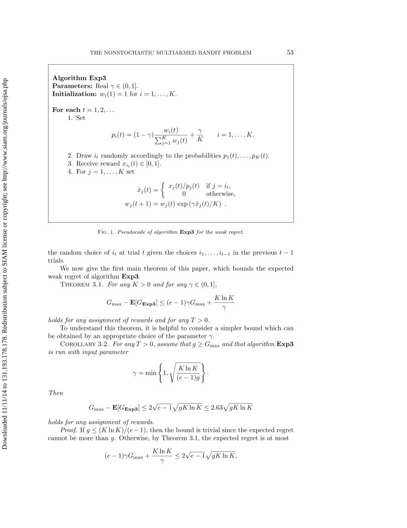
3. Upper bounds on the weak regret. In this section we present and analyzeour simplest player algorithm, Exp3 (which stands for “exponential-weight algorithmfor exploration and exploitation”). We will show a bound on the expected regret ofExp3 with respect to the single best action. In the next sections, we will greatlystrengthen this result.
The algorithm Exp3, described in Figure 1, is a variant of the algorithm Hedgeintroduced by Freund and Schapire [6] for solving a different worst-case sequentialallocation problem. On each time step t, Exp3 draws an action it according to thedistribution p1(t), . . . , pK(t). This distribution is a mixture of the uniform distributionand a distribution which assigns to each action a probability mass exponential inthe estimated cumulative reward for that action. Intuitively, mixing in the uniformdistribution is done to make sure that the algorithm tries out all K actions and getsgood estimates of the rewards for each. Otherwise, the algorithm might miss a goodaction because the initial rewards it observes for this action are low and large rewardsthat occur later are not observed because the action is not selected.
For the drawn action it, Exp3 sets the estimated reward xit(t) to xit(t)/pit(t).Dividing the actual gain by the probability that the action was chosen compensatesthe reward of actions that are unlikely to be chosen. This choice of estimated rewardsguarantees that their expectations are equal to the actual rewards for each action;that is, E[xj(t) | i1, . . . , it−1] = xj(t), where the expectation is taken with respect to
Dow
nloa
ded
11/1
1/14
to 1
31.1
93.1
78.1
78. R
edis
trib
utio
n su
bjec
t to
SIA
M li
cens
e or
cop
yrig
ht; s
ee h
ttp://
ww
w.s
iam
.org
/jour
nals
/ojs
a.ph
p
THE NONSTOCHASTIC MULTIARMED BANDIT PROBLEM 53
Algorithm Exp3Parameters: Real γ ∈ (0, 1].Initialization: wi(1) = 1 for i = 1, . . . ,K.
For each t = 1, 2, . . .1. Set
pi(t) = (1− γ)wi(t)∑Kj=1 wj(t)
+γ
Ki = 1, . . . ,K.
2. Draw it randomly accordingly to the probabilities p1(t), . . . , pK(t).3. Receive reward xit(t) ∈ [0, 1].4. For j = 1, . . . ,K set
xj(t) =
xj(t)/pj(t) if j = it,
0 otherwise,
wj(t + 1) = wj(t) exp (γxj(t)/K) .
Fig. 1. Pseudocode of algorithm Exp3 for the weak regret.
the random choice of it at trial t given the choices i1, . . . , it−1 in the previous t − 1trials.
We now give the first main theorem of this paper, which bounds the expectedweak regret of algorithm Exp3.
Theorem 3.1. For any K > 0 and for any γ ∈ (0, 1],
Gmax −E[GExp3] ≤ (e− 1)γGmax +K lnK
γ
holds for any assignment of rewards and for any T > 0.To understand this theorem, it is helpful to consider a simpler bound which can
be obtained by an appropriate choice of the parameter γ.Corollary 3.2. For any T > 0, assume that g ≥ Gmax and that algorithm Exp3
is run with input parameter
γ = min
1,
√K lnK
(e− 1)g
.
Then
Gmax −E[GExp3] ≤ 2√e− 1
√gK lnK ≤ 2.63
√gK lnK
holds for any assignment of rewards.Proof. If g ≤ (K lnK)/(e− 1), then the bound is trivial since the expected regret
cannot be more than g. Otherwise, by Theorem 3.1, the expected regret is at most
(e− 1)γGmax +K lnK
γ≤ 2
√e− 1
√gK lnK,
Dow
nloa
ded
11/1
1/14
to 1
31.1
93.1
78.1
78. R
edis
trib
utio
n su
bjec
t to
SIA
M li
cens
e or
cop
yrig
ht; s
ee h
ttp://
ww
w.s
iam
.org
/jour
nals
/ojs
a.ph
p
54 AUER, CESA-BIANCHI, FREUND, AND SCHAPIRE
as desired.To apply Corollary 3.2, it is necessary that an upper bound g on Gmax(T ) be
available for tuning γ. For example, if the time horizon T is known, then, since noaction can have payoff greater than 1 on any trial, we can use g = T as an upperbound. In section 4, we give a technique that does not require prior knowledge ofsuch an upper bound, yielding a result which uniformly holds over T .
If the rewards xi(t) are in the range [a, b], a < b, then Exp3 can be used after therewards have been translated and rescaled to the range [0, 1]. Applying Corollary 3.2with g = T gives the bound (b−a)2
√e− 1
√TK lnK on the regret. For instance, this
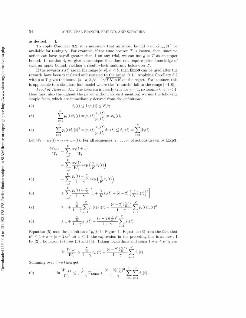
is applicable to a standard loss model where the “rewards” fall in the range [−1, 0].Proof of Theorem 3.1. The theorem is clearly true for γ = 1, so assume 0 < γ < 1.
Here (and also throughout the paper without explicit mention) we use the followingsimple facts, which are immediately derived from the definitions:
xi(t) ≤ 1/pi(t) ≤ K/γ,(2)K∑i=1
pi(t)xi(t) = pit(t)xit(t)
pit(t)= xit(t),(3)
K∑i=1
pi(t)xi(t)2 = pit(t)
xit(t)
pit(t)xit(t) ≤ xit(t) =
K∑i=1
xi(t).(4)
Let Wt = w1(t)+ · · ·+wK(t). For all sequences i1, . . . , iT of actions drawn by Exp3,
Wt+1
Wt=
K∑i=1
wi(t + 1)
Wt
=
K∑i=1
wi(t)
Wtexp
( γ
Kxi(t)
)
=
K∑i=1
pi(t)− γK
1− γexp
( γ
Kxi(t)
)(5)
≤K∑i=1
pi(t)− γK
1− γ
[1 +
γ
Kxi(t) + (e− 2)
( γ
Kxi(t)
)2]
(6)
≤ 1 +γK
1− γ
K∑i=1
pi(t)xi(t) +(e− 2)( γ
K )2
1− γ
K∑i=1
pi(t)xi(t)2(7)
≤ 1 +γK
1− γxit(t) +
(e− 2)( γK )2
1− γ
K∑i=1
xi(t).(8)
Equation (5) uses the definition of pi(t) in Figure 1. Equation (6) uses the fact thatex ≤ 1 + x + (e − 2)x2 for x ≤ 1; the expression in the preceding line is at most 1by (2). Equation (8) uses (3) and (4). Taking logarithms and using 1 + x ≤ ex gives
lnWt+1
Wt≤
γK
1− γxit(t) +
(e− 2)( γK )2
1− γ
K∑i=1
xi(t).
Summing over t we then get
lnWT+1
W1≤
γK
1− γGExp3 +
(e− 2)( γK )2
1− γ
T∑t=1
K∑i=1
xi(t) .(9)
Dow
nloa
ded
11/1
1/14
to 1
31.1
93.1
78.1
78. R
edis
trib
utio
n su
bjec
t to
SIA
M li
cens
e or
cop
yrig
ht; s
ee h
ttp://
ww
w.s
iam
.org
/jour
nals
/ojs
a.ph
p
THE NONSTOCHASTIC MULTIARMED BANDIT PROBLEM 55
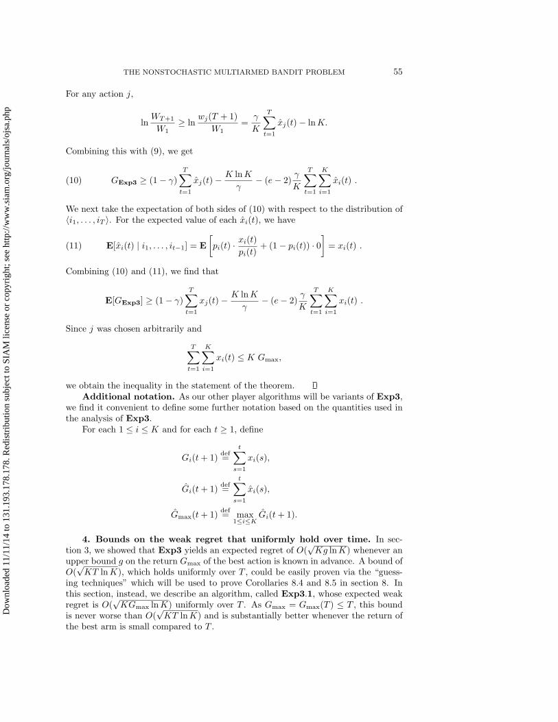
For any action j,
lnWT+1
W1≥ ln
wj(T + 1)
W1=
γ
K
T∑t=1
xj(t)− lnK.
Combining this with (9), we get
GExp3 ≥ (1− γ)
T∑t=1
xj(t)− K lnK
γ− (e− 2)
γ
K
T∑t=1
K∑i=1
xi(t) .(10)
We next take the expectation of both sides of (10) with respect to the distribution of〈i1, . . . , iT 〉. For the expected value of each xi(t), we have
E[xi(t) | i1, . . . , it−1] = E
[pi(t) · xi(t)
pi(t)+ (1− pi(t)) · 0
]= xi(t) .(11)
Combining (10) and (11), we find that
E[GExp3] ≥ (1− γ)
T∑t=1
xj(t)− K lnK
γ− (e− 2)
γ
K
T∑t=1
K∑i=1
xi(t) .
Since j was chosen arbitrarily and
T∑t=1
K∑i=1
xi(t) ≤ K Gmax,
we obtain the inequality in the statement of the theorem.Additional notation. As our other player algorithms will be variants of Exp3,
we find it convenient to define some further notation based on the quantities used inthe analysis of Exp3.
For each 1 ≤ i ≤ K and for each t ≥ 1, define
Gi(t + 1)def=
t∑s=1
xi(s),
Gi(t + 1)def=
t∑s=1
xi(s),
Gmax(t + 1)def= max
1≤i≤KGi(t + 1).
4. Bounds on the weak regret that uniformly hold over time. In sec-tion 3, we showed that Exp3 yields an expected regret of O(
√Kg lnK) whenever an
upper bound g on the return Gmax of the best action is known in advance. A bound ofO(
√KT lnK), which holds uniformly over T , could be easily proven via the “guess-
ing techniques” which will be used to prove Corollaries 8.4 and 8.5 in section 8. Inthis section, instead, we describe an algorithm, called Exp3.1, whose expected weakregret is O(
√KGmax lnK) uniformly over T . As Gmax = Gmax(T ) ≤ T , this bound
is never worse than O(√KT lnK) and is substantially better whenever the return of
the best arm is small compared to T .
Dow
nloa
ded
11/1
1/14
to 1
31.1
93.1
78.1
78. R
edis
trib
utio
n su
bjec
t to
SIA
M li
cens
e or
cop
yrig
ht; s
ee h
ttp://
ww
w.s
iam
.org
/jour
nals
/ojs
a.ph
p
56 AUER, CESA-BIANCHI, FREUND, AND SCHAPIRE
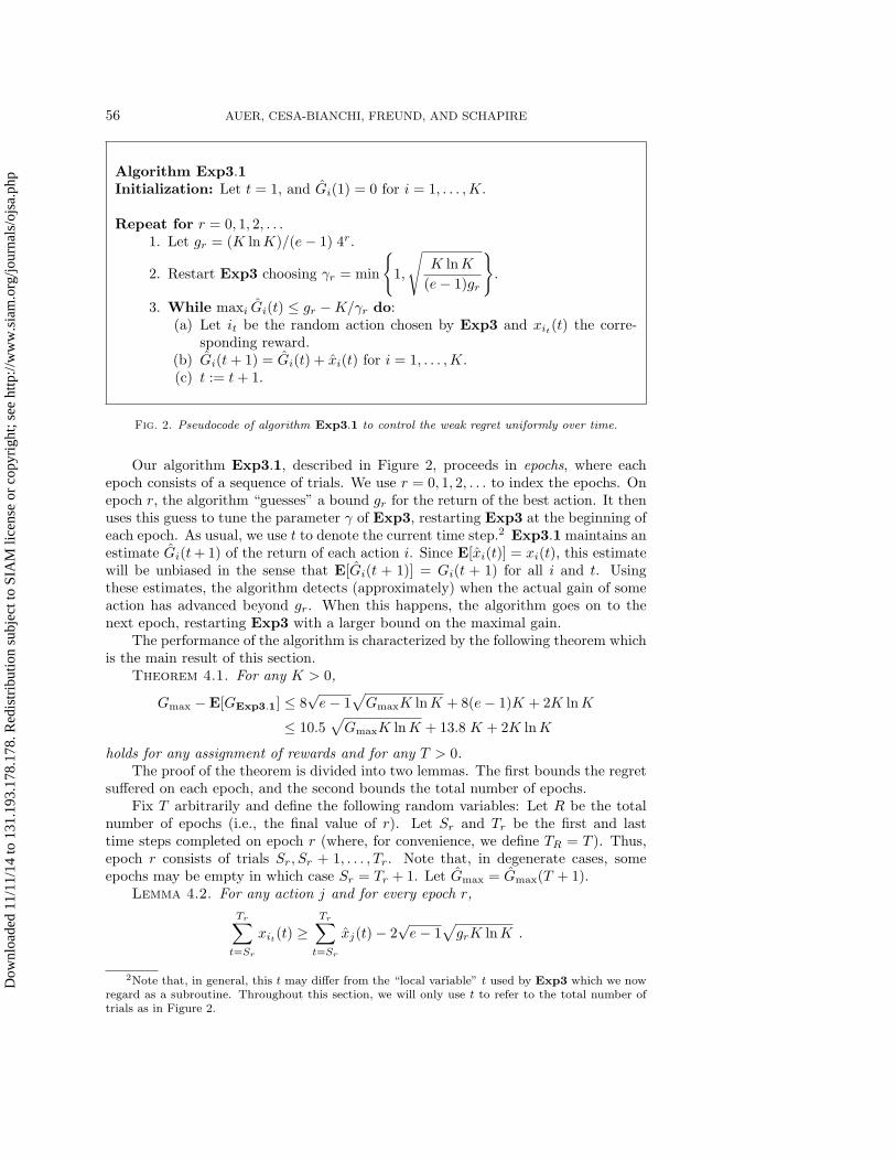
Algorithm Exp3.1Initialization: Let t = 1, and Gi(1) = 0 for i = 1, . . . ,K.
Repeat for r = 0, 1, 2, . . .1. Let gr = (K lnK)/(e− 1) 4r.
2. Restart Exp3 choosing γr = min
1,
√K lnK
(e− 1)gr
.
3. While maxi Gi(t) ≤ gr −K/γr do:(a) Let it be the random action chosen by Exp3 and xit(t) the corre-
sponding reward.(b) Gi(t + 1) = Gi(t) + xi(t) for i = 1, . . . ,K.(c) t := t + 1.
Fig. 2. Pseudocode of algorithm Exp3.1 to control the weak regret uniformly over time.
Our algorithm Exp3.1, described in Figure 2, proceeds in epochs, where eachepoch consists of a sequence of trials. We use r = 0, 1, 2, . . . to index the epochs. Onepoch r, the algorithm “guesses” a bound gr for the return of the best action. It thenuses this guess to tune the parameter γ of Exp3, restarting Exp3 at the beginning ofeach epoch. As usual, we use t to denote the current time step.2 Exp3.1 maintains anestimate Gi(t+1) of the return of each action i. Since E[xi(t)] = xi(t), this estimatewill be unbiased in the sense that E[Gi(t + 1)] = Gi(t + 1) for all i and t. Usingthese estimates, the algorithm detects (approximately) when the actual gain of someaction has advanced beyond gr. When this happens, the algorithm goes on to thenext epoch, restarting Exp3 with a larger bound on the maximal gain.
The performance of the algorithm is characterized by the following theorem whichis the main result of this section.
Theorem 4.1. For any K > 0,
Gmax −E[GExp3.1] ≤ 8√e− 1
√GmaxK lnK + 8(e− 1)K + 2K lnK
≤ 10.5√
GmaxK lnK + 13.8 K + 2K lnK
holds for any assignment of rewards and for any T > 0.The proof of the theorem is divided into two lemmas. The first bounds the regret
suffered on each epoch, and the second bounds the total number of epochs.Fix T arbitrarily and define the following random variables: Let R be the total
number of epochs (i.e., the final value of r). Let Sr and Tr be the first and lasttime steps completed on epoch r (where, for convenience, we define TR = T ). Thus,epoch r consists of trials Sr, Sr + 1, . . . , Tr. Note that, in degenerate cases, someepochs may be empty in which case Sr = Tr + 1. Let Gmax = Gmax(T + 1).
Lemma 4.2. For any action j and for every epoch r,
Tr∑t=Sr
xit(t) ≥Tr∑
t=Sr
xj(t)− 2√e− 1
√grK lnK .
2Note that, in general, this t may differ from the “local variable” t used by Exp3 which we nowregard as a subroutine. Throughout this section, we will only use t to refer to the total number oftrials as in Figure 2.
Dow
nloa
ded
11/1
1/14
to 1
31.1
93.1
78.1
78. R
edis
trib
utio
n su
bjec
t to
SIA
M li
cens
e or
cop
yrig
ht; s
ee h
ttp://
ww
w.s
iam
.org
/jour
nals
/ojs
a.ph
p
THE NONSTOCHASTIC MULTIARMED BANDIT PROBLEM 57
Proof. If Sr > Tr (so that no trials occur on epoch r), then the lemma holdstrivially since both summations will be equal to zero. Assume then that Sr ≤ Tr. Letg = gr and γ = γr. We use (10) from the proof of Theorem 3.1:
Tr∑t=Sr
xit(t) ≥Tr∑
t=Sr
xj(t)− γ
Tr∑t=1
xj(t)− K lnK
γ− (e− 2)
γ
K
Tr∑t=Sr
K∑i=1
xi(t) .
From the definition of the termination condition we know that Gi(Tr) ≤ g − K/γ.Using (2), we get xi(t) ≤ K/γ. This implies that Gi(Tr + 1) ≤ g for all i. Thus,
Tr∑t=Sr
xit(t) ≥Tr∑
t=Sr
xj(t)− g (γ + γ(e− 2))− K lnK
γ.
By our choice for γ, we get the statement of the lemma.The next lemma gives an implicit upper bound on the number of epochs R. Let
c = (K lnK)/(e− 1).Lemma 4.3. The number of epochs R satisfies
2R−1 ≤ K
c+
√Gmax
c+
1
2.
Proof. If R = 0, then the bound holds trivially. So assume R ≥ 1. Let z = 2R−1.Because epoch R− 1 was completed, by the termination condition,
Gmax ≥ Gmax(TR−1 + 1) > gR−1 − K
γR−1= c 4R−1 −K 2R−1 = cz2 −Kz .(12)
Suppose the claim of the lemma is false. Then z > K/c +
√Gmax/c. Since the
function cx2 −Kx is increasing for x > K/(2c), this implies that
cz2 −Kz > c
K
c+
√Gmax
c
2
−K
K
c+
√Gmax
c
= K
√Gmax
c+ Gmax ,
contradicting (12).Proof of Theorem 4.1. Using the lemmas, we have that
GExp3.1 =
T∑t=1
xit(t) =
R∑r=0
Tr∑t=Sr
xit(t)
≥ maxj
R∑r=0
(Tr∑
t=Sr
xj(t)− 2√e− 1
√grK lnK
)
= maxj
Gj(T + 1)− 2K lnK
R∑r=0
2r
= Gmax − 2K lnK(2R+1 − 1)
≥ Gmax + 2K lnK − 8K lnK
K
c+
√Gmax
c+
1
2
= Gmax − 2K lnK − 8(e− 1)K − 8√e− 1
√GmaxK lnK .(13)
Dow
nloa
ded
11/1
1/14
to 1
31.1
93.1
78.1
78. R
edis
trib
utio
n su
bjec
t to
SIA
M li
cens
e or
cop
yrig
ht; s
ee h
ttp://
ww
w.s
iam
.org
/jour
nals
/ojs
a.ph
p
58 AUER, CESA-BIANCHI, FREUND, AND SCHAPIRE
Here, we used Lemma 4.2 for the first inequality and Lemma 4.3 for the secondinequality. The other steps follow from definitions and simple algebra.
Let f(x) = x−a√x− b for x ≥ 0, where a = 8
√e− 1
√K lnK and b = 2K lnK+
8(e− 1)K. Taking expectations of both sides of (13) gives
E[GExp3.1] ≥ E[f(Gmax)] .(14)
Since the second derivative of f is positive for x > 0, f is convex so that, by Jensen’sinequality,
E[f(Gmax)] ≥ f(E[Gmax]) .(15)
Note that
E[Gmax] = E
[max
jGj(T + 1)
]≥ max
jE[Gj(T + 1)] = max
j
T∑t=1
xj(t) = Gmax .
The function f is increasing if and only if x > a2/4. Therefore, if Gmax > a2/4, thenf(E[Gmax]) ≥ f(Gmax). Combined with (14) and (15), this gives that E[GExp3.1] ≥f(Gmax), which is equivalent to the statement of the theorem. On the other hand, ifGmax ≤ a2/4, then, because f is nonincreasing on [0, a2/4],
f(Gmax) ≤ f(0) = −b ≤ 0 ≤ E[GExp3.1],
so the theorem trivially follows in this case as well.
5. Lower bounds on the weak regret. In this section, we state a lower boundon the expected weak regret of any player. More precisely, for any choice of the timehorizon T we show that there exists a strategy for assigning the rewards to the actionssuch that the expected weak regret of any player algorithm is Ω(
√KT ). Observe that
this does not match the upper bound for our algorithms Exp3 and Exp3.1 (seeCorollary 3.2 and Theorem 4.1); it is an open problem to close this gap.
Our lower bound is proven using the classical (statistical) bandit model with acrucial difference: the reward distribution depends on the number K of actions andon the time horizon T . This dependence is the reason why our lower bound does notcontradict the upper bounds of the form O(lnT ) for the classical bandit model [14].There, the distribution over the rewards is fixed as T → ∞.
Note that our lower bound has a considerably stronger dependence on the num-ber K of action than the lower bound Θ(
√T lnK), which could have been directly
proven from the results in [3, 6]. Specifically, our lower bound implies that no upperbound is possible of the form O(Tα(lnK)β), where 0 ≤ α < 1, β > 0.
Theorem 5.1. For any number of actions K ≥ 2 and for any time horizon T ,there exists a distribution over the assignment of rewards such that the expected weakregret of any algorithm (where the expectation is taken with respect to both the ran-domization over rewards and the algorithm’s internal randomization) is at least
1
20min
√KT, T.
The proof is given in Appendix A.The lower bound implies, of course, that for any algorithm there is a particular
choice of rewards that will cause the expected weak regret (where the expectation isnow with respect to the algorithm’s internal randomization only) to be larger thanthis value.
Dow
nloa
ded
11/1
1/14
to 1
31.1
93.1
78.1
78. R
edis
trib
utio
n su
bjec
t to
SIA
M li
cens
e or
cop
yrig
ht; s
ee h
ttp://
ww
w.s
iam
.org
/jour
nals
/ojs
a.ph
p
THE NONSTOCHASTIC MULTIARMED BANDIT PROBLEM 59
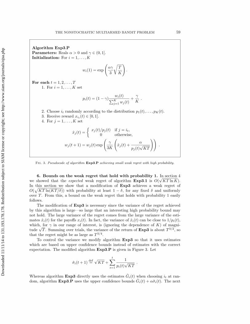
Algorithm Exp3.PParameters: Reals α > 0 and γ ∈ (0, 1].Initialization: For i = 1, . . . ,K
wi(1) = exp
(αγ
3
√T
K
).
For each t = 1, 2, . . . , T1. For i = 1, . . . ,K set
pi(t) = (1− γ)wi(t)∑Kj=1 wj(t)
+γ
K.
2. Choose it randomly according to the distribution p1(t), . . . , pK(t).3. Receive reward xit(t) ∈ [0, 1].4. For j = 1, . . . ,K set
xj(t) =
xj(t)/pj(t) if j = it,
0 otherwise,
wj(t + 1) = wj(t) exp
(γ
3K
(xj(t) +
α
pj(t)√KT
)).
Fig. 3. Pseudocode of algorithm Exp3.P achieving small weak regret with high probability.
6. Bounds on the weak regret that hold with probability 1. In section 4we showed that the expected weak regret of algorithm Exp3.1 is O(
√KT lnK).
In this section we show that a modification of Exp3 achieves a weak regret ofO(√
KT ln(KT/δ)) with probability at least 1 − δ, for any fixed δ and uniformlyover T . From this, a bound on the weak regret that holds with probability 1 easilyfollows.
The modification of Exp3 is necessary since the variance of the regret achievedby this algorithm is large—so large that an interesting high probability bound maynot hold. The large variance of the regret comes from the large variance of the esti-mates xi(t) for the payoffs xi(t). In fact, the variance of xi(t) can be close to 1/pi(t),which, for γ in our range of interest, is (ignoring the dependence of K) of magni-tude
√T . Summing over trials, the variance of the return of Exp3 is about T 3/2, so
that the regret might be as large as T 3/4.To control the variance we modify algorithm Exp3 so that it uses estimates
which are based on upper confidence bounds instead of estimates with the correctexpectation. The modified algorithm Exp3.P is given in Figure 3. Let
σi(t + 1)def=
√KT +
t∑s=1
1
pi(t)√KT
.
Whereas algorithm Exp3 directly uses the estimates Gi(t) when choosing it at ran-dom, algorithm Exp3.P uses the upper confidence bounds Gi(t) + ασi(t). The next
Dow
nloa
ded
11/1
1/14
to 1
31.1
93.1
78.1
78. R
edis
trib
utio
n su
bjec
t to
SIA
M li
cens
e or
cop
yrig
ht; s
ee h
ttp://
ww
w.s
iam
.org
/jour
nals
/ojs
a.ph
p
60 AUER, CESA-BIANCHI, FREUND, AND SCHAPIRE
lemma shows that, for appropriate α, these are indeed upper confidence bounds. Fixsome time horizon T . In what follows, we will use σi to denote σi(T + 1) and Gi todenote Gi(T + 1).
Lemma 6.1. If 2√
ln(KT/δ) ≤ α ≤ 2√KT , then
P∃i : Gi + ασi < Gi
≤ δ.
Proof. Fix some i and set
stdef=
α
2σi(t + 1).
Since α ≤ 2√KT and σi(t + 1) ≥ √
KT , we have st ≤ 1. Now
PGi + ασi < Gi
= P
T∑
t=1
(xi(t)− xi(t))− α
2σi >
α
2σi
≤ P
sT
T∑t=1
(xi(t)− xi(t)− α
2pi(t)√KT
)>
α2
4
(16)
= P
exp
(sT
T∑t=1
(xi(t)− xi(t)− α
2pi(t)√KT
))> exp
(α2
4
)
≤ e−α2/4E
[exp
(sT
T∑t=1
(xi(t)− xi(t)− α
2pi(t)√KT
))],(17)
where in step (16) we multiplied both sides by sT and used σi ≥∑T
t=1 1/(pi(t)√KT ),
while in step (17) we used Markov’s inequality. For t = 1, . . . , T set
Ztdef= exp
(st
t∑τ=1
(xi(τ)− xi(τ)− α
2pi(τ)√KT
)).
Then, for t = 2, . . . , T
Zt = exp
(st
(xi(t)− xi(t)− α
2pi(t)√KT
))· (Zt−1)
stst−1 .
Denote by Et [Zt] = E [Zt | i1, . . . , it−1] the expectation of Zt with respect to therandom choice in trial t and conditioned on the past t− 1 trials. Note that when thepast t− 1 trials are fixed the only random quantities in Zt are the xi(t)’s. Note alsothat xi(t)− xi(t) ≤ 1 and that
Et
[(xi(t)− xi(t))
2]= Et
[xi(t)
2]− xi(t)
2
≤ Et
[xi(t)
2]
=xi(t)
2
pi(t)≤ 1
pi(t).(18)
Dow
nloa
ded
11/1
1/14
to 1
31.1
93.1
78.1
78. R
edis
trib
utio
n su
bjec
t to
SIA
M li
cens
e or
cop
yrig
ht; s
ee h
ttp://
ww
w.s
iam
.org
/jour
nals
/ojs
a.ph
p
THE NONSTOCHASTIC MULTIARMED BANDIT PROBLEM 61
Hence, for each t = 2, . . . , T
Et [Zt] ≤ Et
[exp st
(xi(t)− xi(t)− st
pi(t)
)](Zt−1)
stst−1(19)
≤ Et
[1 + st(xi(t)− xi(t)) + s2
t (xi(t)− xi(t))2]exp
(− s2
t
pi(t)
)(Zt−1)
stst−1(20)
≤ (1 + s2
t/pi(t))exp
(− s2
t
pi(t)
)(Zt−1)
stst−1(21)
≤ (Zt−1)st
st−1(22)
≤ 1 + Zt−1.(23)
Equation (19) uses
α
2pi(t)√KT
≥ α
2pi(t)σi(t + 1)=
stpi(t)
since σi(t + 1) ≥ √KT . Equation (20) uses ea ≤ 1 + a + a2 for a ≤ 1. Equation (21)
uses Et [xi(t)] = xi(t). Equation (22) uses 1 + x ≤ ex for any real x. Equation (23)uses st ≤ st−1 and zu ≤ 1+ z for any z > 0 and u ∈ [0, 1]. Observing that E [Z1] ≤ 1,we get by induction that E[ZT ] ≤ T , and the lemma follows by our choice of α.
The next lemma shows that the return achieved by algorithm Exp3.P is close toits upper confidence bounds. Let
Udef= max
1≤i≤K
(Gi + ασi
).
Lemma 6.2. If α ≤ 2√KT , then
GExp3.P ≥(1− 5γ
3
)U − 3
γK lnK − 2α
√KT − 2α2 .
Proof. We proceed as in the analysis of algorithm Exp3. Set η = γ/(3K) andconsider any sequence i1, . . . , iT of actions chosen by Exp3.P. As xi(t) ≤ K/γ,pi(t) ≥ γ/K, and α ≤ 2
√KT , we have
ηxi(t) +αη
pi(t)√KT
≤ 1 .
Therefore,
Wt+1
Wt=
K∑i=1
wi(t + 1)
Wt
=
K∑i=1
wi(t)
Wtexp
(ηxi(t) +
αη
pi(t)√KT
)
=K∑i=1
pi(t)− γ/K
1− γexp
(ηxi(t) +
αη
pi(t)√KT
)
≤K∑i=1
pi(t)− γ/K
1− γ
[1 + ηxi(t) +
αη
pi(t)√KT
+ 2η2xi(t)2 +
2α2η2
pi(t)2KT
]
Dow
nloa
ded
11/1
1/14
to 1
31.1
93.1
78.1
78. R
edis
trib
utio
n su
bjec
t to
SIA
M li
cens
e or
cop
yrig
ht; s
ee h
ttp://
ww
w.s
iam
.org
/jour
nals
/ojs
a.ph
p
62 AUER, CESA-BIANCHI, FREUND, AND SCHAPIRE
≤ 1 +η
1− γ
K∑i=1
pi(t)xi(t) +αη
1− γ
K∑i=1
1√KT
+2η2
1− γ
K∑i=1
pi(t)xi(t)2 +
2α2η2
1− γ
K∑i=1
1
pi(t)KT
≤ 1 +η
1− γxit(t) +
αη
1− γ
√K
T+
2η2
1− γ
K∑i=1
xi(t) +2α2η
1− γ
1
T.
The second inequality uses ea ≤ 1+a+a2 for a ≤ 1, and (a+ b)2 ≤ 2(a2 + b2) for anya, b. The last inequality uses (2), (3), and (4). Taking logarithms, using ln(1+x) ≤ x,and summing over t = 1, . . . , T , we get
lnWT+1
W1≤ η
1− γGExp3.P +
αη
1− γ
√KT +
2η2
1− γ
K∑i=1
Gi +2α2η
1− γ.
Since
lnW1 = αη√KT + lnK
and for any j
lnWT+1 ≥ lnwj(T + 1) ≥ ηGj + αησj ,
this implies
GExp3.P ≥ (1− γ)(Gj + ασj
)− 1
ηlnK − 2α
√KT − 2η
K∑i=1
Gi − 2α2
for any j. Finally, using η = γ/(3K) and
K∑i=1
Gi ≤ KU
yields the lemma.Combining Lemmas 6.1 and 6.2 gives the main result of this section.Theorem 6.3. For any fixed T > 0, for all K ≥ 2 and for all δ > 0, if
γ = min
3
5, 2
√3
5
K lnK
T
and α = 2
√ln(KT/δ) ,
then
Gmax −GExp3.P ≤ 4
√KT ln
KT
δ+ 4
√5
3KT lnK + 8 ln
KT
δ
holds for any assignment of rewards with probability at least 1− δ.Proof. We assume without loss of generality that T ≥ (20/3)K lnK and that
δ ≥ KTe−KT . If either of these conditions do not hold, then the theorem holdstrivially. Note that T ≥ (20/3)K lnK ensures γ ≤ 3/5. Note also that δ ≥ KTe−KT
Dow
nloa
ded
11/1
1/14
to 1
31.1
93.1
78.1
78. R
edis
trib
utio
n su
bjec
t to
SIA
M li
cens
e or
cop
yrig
ht; s
ee h
ttp://
ww
w.s
iam
.org
/jour
nals
/ojs
a.ph
p
THE NONSTOCHASTIC MULTIARMED BANDIT PROBLEM 63
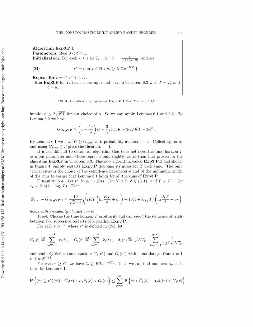
Algorithm Exp3.P.1Parameters: Real 0 < δ < 1.Initialization: For each r ≥ 1 let Tr = 2r, δr = δ
(r+1)(r+2) , and set
r∗ = minr ∈ N : δr ≥ KTre−KTr.(24)
Repeat for r = r∗, r∗ + 1, . . .Run Exp3.P for Tr trials choosing α and γ as in Theorem 6.3 with T = Tr and
δ = δr.
Fig. 4. Pseudocode of algorithm Exp3.P.1 (see Theorem 6.4).
implies α ≤ 2√KT for our choice of α. So we can apply Lemmas 6.1 and 6.2. By
Lemma 6.2 we have
GExp3.P ≥(1− 5γ
3
)U − 3
γK lnK − 2α
√KT − 2α2 .
By Lemma 6.1 we have U ≥ Gmax with probability at least 1 − δ. Collecting termsand using Gmax ≤ T gives the theorem.
It is not difficult to obtain an algorithm that does not need the time horizon Tas input parameter and whose regret is only slightly worse than that proven for thealgorithm Exp3.P in Theorem 6.3. This new algorithm, called Exp3.P.1 and shownin Figure 4, simply restarts Exp3.P doubling its guess for T each time. The onlycrucial issue is the choice of the confidence parameter δ and of the minimum lengthof the runs to ensure that Lemma 6.1 holds for all the runs of Exp3.P.
Theorem 6.4. Let r∗ be as in (24). Let K ≥ 2, δ ∈ (0, 1), and T ≥ 2r∗. Let
cT = 2 ln(2 + log2 T ). Then
Gmax −GExp3.P.1 ≤ 10√2− 1
√2KT
(ln
KT
δ+ cT
)+ 10(1 + log2 T )
(ln
KT
δ+ cT
)
holds with probability at least 1− δ.Proof. Choose the time horizon T arbitrarily and call epoch the sequence of trials
between two successive restarts of algorithm Exp3.P.For each r > r∗, where r∗ is defined in (24), let
Gi(r)def=
2r+1∑t=2r+1
xi(t) , Gi(r)def=
2r+1∑t=2r+1
xi(t) , σi(r)def=√
KTr+
2r+1∑t=2r+1
1
pi(t)√KTr
and similarly define the quantities Gi(r∗) and Gi(r
∗) with sums that go from t = 1to t = 2r
∗+1.For each r ≥ r∗, we have δr ≥ KTre
−KTr . Thus we can find numbers αr suchthat, by Lemma 6.1,
P(∃r ≥ r∗)(∃i) : Gi(r) + αrσi(r) < Gi(r)
≤
∞∑r=r∗
P∃i : Gi(r) + αrσi(r) < Gi(r)
Dow
nloa
ded
11/1
1/14
to 1
31.1
93.1
78.1
78. R
edis
trib
utio
n su
bjec
t to
SIA
M li
cens
e or
cop
yrig
ht; s
ee h
ttp://
ww
w.s
iam
.org
/jour
nals
/ojs
a.ph
p
64 AUER, CESA-BIANCHI, FREUND, AND SCHAPIRE
≤∞∑r=0
δ
(r + 1)(r + 2)
= δ .
We now apply Theorem 6.3 to each epoch. Since T ≥ 2r∗, there is an * ≥ 1 such that
2r∗+−1 ≤ T =
−1∑r=0
2r∗+r < 2r
∗+ .
With probability at least 1−δ over the random draw of Exp3.P.1’s actions i1, . . . , iT ,
Gmax −GExp3.P.1
≤−1∑r=0
10
[√KTr∗+r ln
KTr∗+r
δr∗+r+ ln
KTr∗+r
δr∗+r
]
≤ 10
[√K ln
KTr∗+−1
δr∗+−1
−1∑r=0
√Tr∗+r + * ln
KTr∗+−1
δr∗+−1
]
≤ 10
[√K ln
KTr∗+−1
δr∗+−1
(2(r∗+)/2
√2− 1
)+ * ln
KTr∗+−1
δr∗+−1
]
≤ 10√2− 1
√2KT
(ln
KT
δ+ cT
)+ 10(1 + log2 T )
(ln
KT
δ+ cT
),
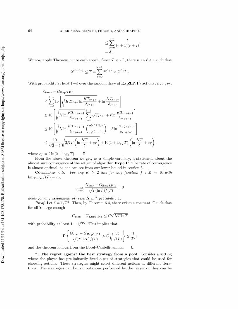
where cT = 2 ln(2 + log2 T ).From the above theorem we get, as a simple corollary, a statement about the
almost sure convergence of the return of algorithm Exp3.P. The rate of convergenceis almost optimal, as one can see from our lower bound in section 5.
Corollary 6.5. For any K ≥ 2 and for any function f : R → R withlimT→∞ f(T ) = ∞,
limT→∞
Gmax −GExp3.P.1√T (lnT )f(T )
= 0
holds for any assignment of rewards with probability 1.Proof. Let δ = 1/T 2. Then, by Theorem 6.4, there exists a constant C such that
for all T large enough
Gmax −GExp3.P.1 ≤ C√KT lnT
with probability at least 1− 1/T 2. This implies that
P
Gmax −GExp3.P.1√
(T lnT )f(T )> C
√K
f(T )
≤ 1
T 2,
and the theorem follows from the Borel–Cantelli lemma.
7. The regret against the best strategy from a pool. Consider a settingwhere the player has preliminarily fixed a set of strategies that could be used forchoosing actions. These strategies might select different actions at different itera-tions. The strategies can be computations performed by the player or they can be
Dow
nloa
ded
11/1
1/14
to 1
31.1
93.1
78.1
78. R
edis
trib
utio
n su
bjec
t to
SIA
M li
cens
e or
cop
yrig
ht; s
ee h
ttp://
ww
w.s
iam
.org
/jour
nals
/ojs
a.ph
p
THE NONSTOCHASTIC MULTIARMED BANDIT PROBLEM 65
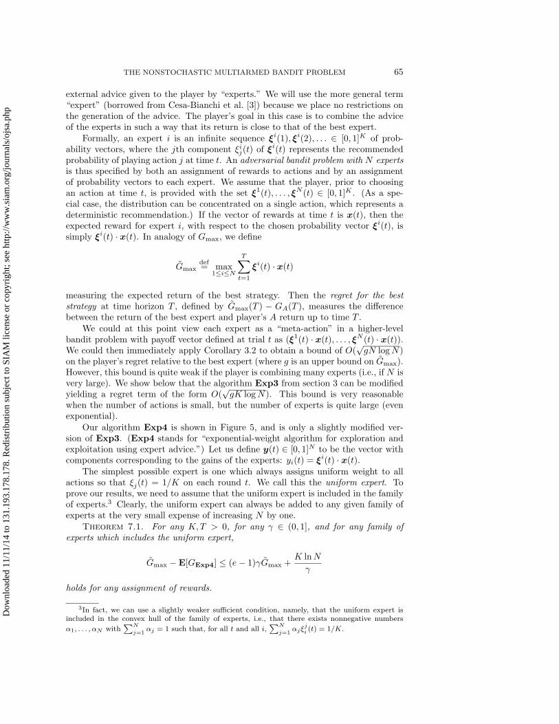
external advice given to the player by “experts.” We will use the more general term“expert” (borrowed from Cesa-Bianchi et al. [3]) because we place no restrictions onthe generation of the advice. The player’s goal in this case is to combine the adviceof the experts in such a way that its return is close to that of the best expert.
Formally, an expert i is an infinite sequence ξi(1), ξi(2), . . . ∈ [0, 1]K of prob-ability vectors, where the jth component ξij(t) of ξi(t) represents the recommendedprobability of playing action j at time t. An adversarial bandit problem with N expertsis thus specified by both an assignment of rewards to actions and by an assignmentof probability vectors to each expert. We assume that the player, prior to choosingan action at time t, is provided with the set ξ1(t), . . . , ξN (t) ∈ [0, 1]K . (As a spe-cial case, the distribution can be concentrated on a single action, which represents adeterministic recommendation.) If the vector of rewards at time t is x(t), then theexpected reward for expert i, with respect to the chosen probability vector ξi(t), issimply ξi(t) · x(t). In analogy of Gmax, we define
Gmaxdef= max
1≤i≤N
T∑t=1
ξi(t) · x(t)
measuring the expected return of the best strategy. Then the regret for the beststrategy at time horizon T , defined by Gmax(T ) − GA(T ), measures the differencebetween the return of the best expert and player’s A return up to time T .
We could at this point view each expert as a “meta-action” in a higher-levelbandit problem with payoff vector defined at trial t as (ξ1(t) · x(t), . . . , ξN (t) · x(t)).We could then immediately apply Corollary 3.2 to obtain a bound of O(
√gN logN)
on the player’s regret relative to the best expert (where g is an upper bound on Gmax).However, this bound is quite weak if the player is combining many experts (i.e., if N isvery large). We show below that the algorithm Exp3 from section 3 can be modifiedyielding a regret term of the form O(
√gK logN). This bound is very reasonable
when the number of actions is small, but the number of experts is quite large (evenexponential).
Our algorithm Exp4 is shown in Figure 5, and is only a slightly modified ver-sion of Exp3. (Exp4 stands for “exponential-weight algorithm for exploration andexploitation using expert advice.”) Let us define y(t) ∈ [0, 1]N to be the vector withcomponents corresponding to the gains of the experts: yi(t) = ξi(t) · x(t).
The simplest possible expert is one which always assigns uniform weight to allactions so that ξj(t) = 1/K on each round t. We call this the uniform expert. Toprove our results, we need to assume that the uniform expert is included in the familyof experts.3 Clearly, the uniform expert can always be added to any given family ofexperts at the very small expense of increasing N by one.
Theorem 7.1. For any K,T > 0, for any γ ∈ (0, 1], and for any family ofexperts which includes the uniform expert,
Gmax −E[GExp4] ≤ (e− 1)γGmax +K lnN
γ
holds for any assignment of rewards.
3In fact, we can use a slightly weaker sufficient condition, namely, that the uniform expert isincluded in the convex hull of the family of experts, i.e., that there exists nonnegative numbers
α1, . . . , αN with∑N
j=1αj = 1 such that, for all t and all i,
∑N
j=1αjξ
ji (t) = 1/K.
Dow
nloa
ded
11/1
1/14
to 1
31.1
93.1
78.1
78. R
edis
trib
utio
n su
bjec
t to
SIA
M li
cens
e or
cop
yrig
ht; s
ee h
ttp://
ww
w.s
iam
.org
/jour
nals
/ojs
a.ph
p
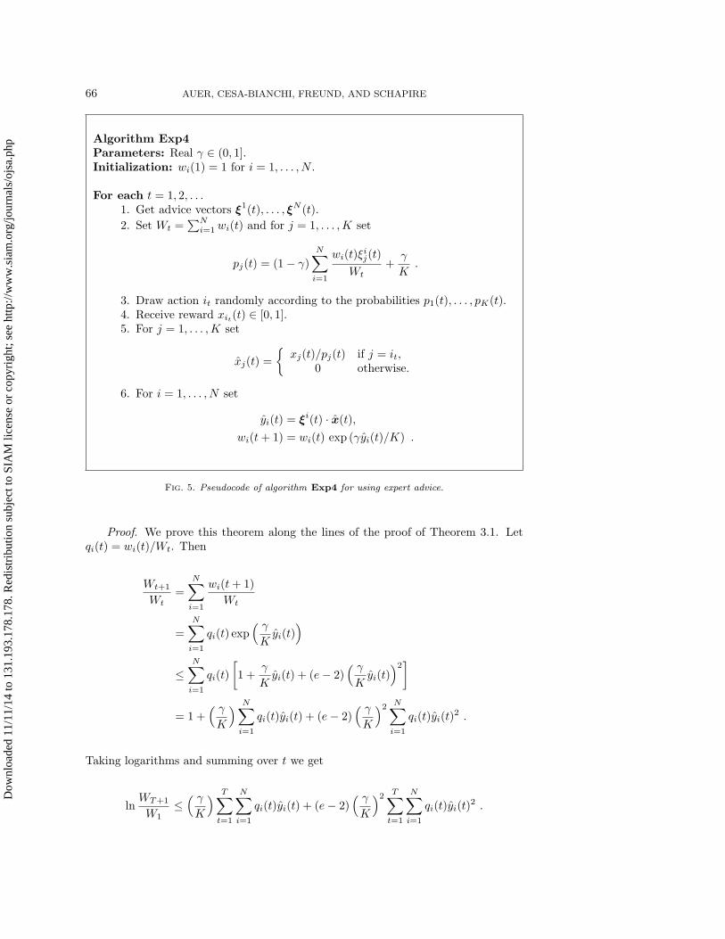
66 AUER, CESA-BIANCHI, FREUND, AND SCHAPIRE
Algorithm Exp4Parameters: Real γ ∈ (0, 1].Initialization: wi(1) = 1 for i = 1, . . . , N .
For each t = 1, 2, . . .1. Get advice vectors ξ1(t), . . . , ξN (t).
2. Set Wt =∑N
i=1 wi(t) and for j = 1, . . . ,K set
pj(t) = (1− γ)
N∑i=1
wi(t)ξij(t)
Wt+
γ
K.
3. Draw action it randomly according to the probabilities p1(t), . . . , pK(t).4. Receive reward xit(t) ∈ [0, 1].5. For j = 1, . . . ,K set
xj(t) =
xj(t)/pj(t) if j = it,
0 otherwise.
6. For i = 1, . . . , N set
yi(t) = ξi(t) · x(t),
wi(t + 1) = wi(t) exp (γyi(t)/K) .
Fig. 5. Pseudocode of algorithm Exp4 for using expert advice.
Proof. We prove this theorem along the lines of the proof of Theorem 3.1. Letqi(t) = wi(t)/Wt. Then
Wt+1
Wt=
N∑i=1
wi(t + 1)
Wt
=
N∑i=1
qi(t) exp( γ
Kyi(t)
)
≤N∑i=1
qi(t)
[1 +
γ
Kyi(t) + (e− 2)
( γ
Kyi(t)
)2]
= 1 +( γ
K
) N∑i=1
qi(t)yi(t) + (e− 2)( γ
K
)2 N∑i=1
qi(t)yi(t)2 .
Taking logarithms and summing over t we get
lnWT+1
W1≤( γ
K
) T∑t=1
N∑i=1
qi(t)yi(t) + (e− 2)( γ
K
)2 T∑t=1
N∑i=1
qi(t)yi(t)2 .
Dow
nloa
ded
11/1
1/14
to 1
31.1
93.1
78.1
78. R
edis
trib
utio
n su
bjec
t to
SIA
M li
cens
e or
cop
yrig
ht; s
ee h
ttp://
ww
w.s
iam
.org
/jour
nals
/ojs
a.ph
p
THE NONSTOCHASTIC MULTIARMED BANDIT PROBLEM 67
Since, for any expert k,
lnWT+1
W1≥ ln
wk(T + 1)
W1=
γ
K
T∑t=1
yk(t)− lnN,
we get
T∑t=1
N∑i=1
qi(t)yi(t) ≥T∑
t=1
yk(t)− K lnN
γ− (e− 2)
γ
K
T∑t=1
N∑i=1
qi(t)yi(t)2 .
Note that
N∑i=1
qi(t)yi(t) =
N∑i=1
qi(t)
K∑
j=1
ξij(t)xj(t)
=K∑j=1
(N∑i=1
qi(t)ξij(t)
)xj(t)
=
K∑j=1
(pj(t)− γ
K
1− γ
)xj(t) ≤ xj(t)
1− γ.
Also,
N∑i=1
qi(t)yi(t)2 =
N∑i=1
qi(t)(ξiit(t)xit(t))
2
≤ xit(t)2 pit(t)
1− γ
≤ xit(t)
1− γ.
Therefore, for all experts k,
GExp4 =
T∑t=1
xit(t) ≥ (1− γ)
T∑t=1
yk(t)− K lnN
γ− (e− 2)
γ
K
T∑t=1
K∑j=1
xj(t) .
We now take expectations of both sides of this inequality. Note that
E[yk(t)] = E
K∑j=1
ξkj (t)xj(t)
=
K∑j=1
ξkj (t)xj(t) = yk(t) .
Further,
1
KE
T∑
t=1
K∑j=1
xj(t)
=
T∑t=1
1
K
K∑j=1
xj(t) ≤ max1≤i≤N
T∑t=1
yi(t) = Gmax
since we have assumed that the uniform expert is included in the family of experts.Combining these facts immediately implies the statement of the theorem.
Dow
nloa
ded
11/1
1/14
to 1
31.1
93.1
78.1
78. R
edis
trib
utio
n su
bjec
t to
SIA
M li
cens
e or
cop
yrig
ht; s
ee h
ttp://
ww
w.s
iam
.org
/jour
nals
/ojs
a.ph
p
68 AUER, CESA-BIANCHI, FREUND, AND SCHAPIRE
Algorithm Exp3.SParameters: Reals γ ∈ (0, 1] and α > 0.Initialization: wi(1) = 1 for i = 1, . . . ,K.
For each t = 1, 2, . . .1. Set
pi(t) = (1− γ)wi(t)∑Kj=1 wj(t)
+γ
K, i = 1, . . . ,K.
2. Draw it according to the probabilities p1(t), . . . , pK(t).3. Receive reward xit(t) ∈ [0, 1].4. For j = 1, . . . ,K set
xj(t) =
xj(t)/pj(t) if j = it,
0 otherwise,
wj(t + 1) = wj(t) exp (γxj(t)/K) +eα
K
K∑i=1
wi(t) .
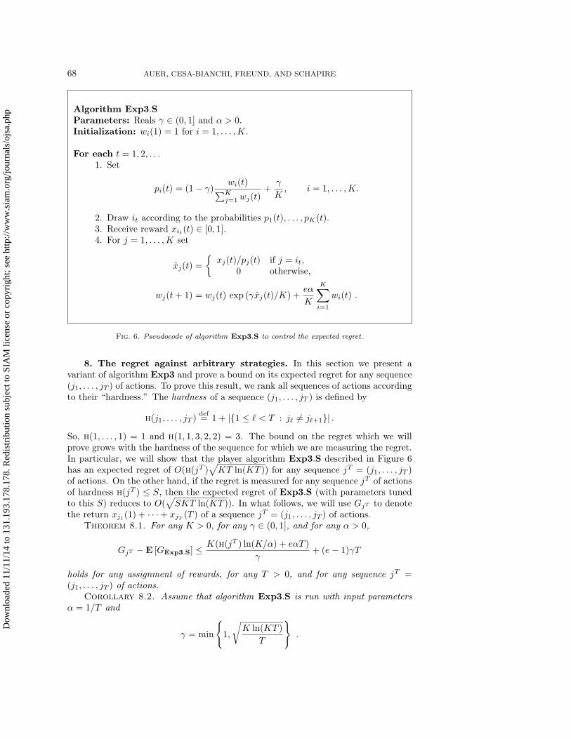
Fig. 6. Pseudocode of algorithm Exp3.S to control the expected regret.
8. The regret against arbitrary strategies. In this section we present avariant of algorithm Exp3 and prove a bound on its expected regret for any sequence(j1, . . . , jT ) of actions. To prove this result, we rank all sequences of actions accordingto their “hardness.” The hardness of a sequence (j1, . . . , jT ) is defined by
h(j1, . . . , jT )def= 1 + |1 ≤ * < T : j = j+1| .
So, h(1, . . . , 1) = 1 and h(1, 1, 3, 2, 2) = 3. The bound on the regret which we willprove grows with the hardness of the sequence for which we are measuring the regret.In particular, we will show that the player algorithm Exp3.S described in Figure 6has an expected regret of O(h(jT )
√KT ln(KT )) for any sequence jT = (j1, . . . , jT )
of actions. On the other hand, if the regret is measured for any sequence jT of actionsof hardness h(jT ) ≤ S, then the expected regret of Exp3.S (with parameters tunedto this S) reduces to O(
√SKT ln(KT )). In what follows, we will use GjT to denote
the return xj1(1) + · · ·+ xjT (T ) of a sequence jT = (j1, . . . , jT ) of actions.Theorem 8.1. For any K > 0, for any γ ∈ (0, 1], and for any α > 0,
GjT −E [GExp3.S] ≤ K(h(jT ) ln(K/α) + eαT )
γ+ (e− 1)γT
holds for any assignment of rewards, for any T > 0, and for any sequence jT =(j1, . . . , jT ) of actions.
Corollary 8.2. Assume that algorithm Exp3.S is run with input parametersα = 1/T and
γ = min
1,
√K ln(KT )
T
.
Dow
nloa
ded
11/1
1/14
to 1
31.1
93.1
78.1
78. R
edis
trib
utio
n su
bjec
t to
SIA
M li
cens
e or
cop
yrig
ht; s
ee h
ttp://
ww
w.s
iam
.org
/jour
nals
/ojs
a.ph
p
THE NONSTOCHASTIC MULTIARMED BANDIT PROBLEM 69
Then
GjT −E [GExp3.S] ≤ h(jT )√
KT ln(KT ) + 2e
√KT
ln(KT )
holds for any sequence jT = (j1, . . . , jT ) of actions.Note that the statement of Corollary 8.2 can be equivalently written as
E [GExp3.S] ≥ maxjT
(GjT − h(jT )
√KT ln(KT )
)
− 2e
√KT
ln(KT ),
revealing that algorithm Exp3.S is able to automatically trade-off between the re-turn GjT of a sequence jT and its hardness h(jT ).
Corollary 8.3. Assume that algorithm Exp3.S is run with input parametersα = 1/T and
γ = min
1,
√K(S ln(KT ) + e)
(e− 1)T
.
Then
GjT −E [GExp3.S] ≤ 2√e− 1
√KT (S ln(KT ) + e)
holds for any sequence jT = (j1, . . . , jT ) of actions such that h(jT ) ≤ S.Proof of Theorem 8.1. Fix any sequence jT = (j1, . . . , jT ) of actions. With a
technique that closely follows the proof of Theorem 3.1, we can prove that for allsequences i1, . . . , iT of actions drawn by Exp3.S,
Wt+1
Wt≤ 1 +
γ/K
1− γxit(t) +
(e− 2)(γ/K)2
1− γ
K∑i=1
xi(t) + eα,(25)
where, as usual, Wt = w1(t)+ · · ·+wK(t). Now let S = h(jT ) and partition (1, . . . , T )in segments
[T1, . . . , T2), [T2, . . . , T3), . . . , [TS , . . . , TS+1),
where T1 = 1, TS+1 = T + 1, and jTs = jTs+1 = · · · = jTs+1−1 for each segment s =1, . . . , S. Fix an arbitrary segment [Ts, Ts+1) and let ∆s = Ts+1 − Ts. Furthermore,let
GExp3.S(s)def=
Ts+1−1∑t=Ts
xit(t) .
Taking logarithms on both sides of (25) and summing over t = Ts, . . . , Ts+1 − 1, weget
lnWTs+1
WTs
≤ γ/K
1− γGExp3.S(s) +
(e− 2)(γ/K)2
1− γ
Ts+1−1∑t=Ts
K∑i=1
xi(t) + eα∆s .(26)
Dow
nloa
ded
11/1
1/14
to 1
31.1
93.1
78.1
78. R
edis
trib
utio
n su
bjec
t to
SIA
M li
cens
e or
cop
yrig
ht; s
ee h
ttp://
ww
w.s
iam
.org
/jour
nals
/ojs
a.ph
p
70 AUER, CESA-BIANCHI, FREUND, AND SCHAPIRE
Now let j be the action such that jTs= · · · = jTs+1−1 = j. Since
wj(Ts+1) ≥ wj(Ts + 1) exp
γ
K
Ts+1−1∑t=Ts+1
xj(t)
≥ eα
KWTs exp
γ
K
Ts+1−1∑t=Ts+1
xj(t)
≥ α
KWTs exp
γ
K
Ts+1−1∑t=Ts
xj(t)
,
where the last step uses γxj(t)/K ≤ 1, we have
lnWTs+1
WTs
≥ lnwj(Ts+1)
WTs
≥ ln( α
K
)+
γ
K
Ts+1−1∑t=Ts
xj(t) .(27)
Piecing together (26) and (27) we get
GExp3.S(s) ≥ (1− γ)
Ts+1−1∑t=Ts
xj(t)−K ln(Kα )
γ− (e− 2)
γ
K
Ts+1−1∑t=Ts
K∑i=1
xi(t)− eαK∆s
γ.
Summing over all segments s = 1, . . . , S, taking expectation with respect to therandom choices of algorithm Exp3.S, and using
G(j1,...,jT ) ≤ T and
T∑t=1
K∑i=1
xi(t) ≤ KT
yields the inequality in the statement of the theorem.If the time horizon T is not known, we can apply techniques similar to those
applied for proving Theorem 6.4 in section 6. More specifically, we introduce a newalgorithm, Exp3.S.1, that runs Exp3.S as a subroutine. Suppose that at each newrun (or epoch) r = 0, 1, . . . , Exp3.S is started with its parameters set as prescribed inCorollary 8.2, where T is set to Tr = 2r, and then stopped after Tr iterations. Clearly,for any fixed sequence jT = (j1, . . . , jT ) of actions, the number of segments (see proofof Theorem 8.1 for a definition of segment) within each epoch r is at most h(jT ).Hence the expected regret of Exp3.S.1 for epoch r is certainly not more than
(h(jT ) + 2e)√
KTr ln(KTr) .
Let * be such that 2 ≤ T < 2+1. Then the last epoch is * ≤ log2 T and the overallregret (over the * + 1 epochs) is at most
(h(jT ) + 2e)
∑r=0
√KTr ln(KTr) ≤ (h(jT ) + 2e)
√K ln(KT)
∑r=0
√Tr .
Finishing up the calculations proves the following.Corollary 8.4.
GjT −E [GExp3.S.1] ≤ h(jT ) + 2e√2− 1
√2KT ln(KT )
Dow
nloa
ded
11/1
1/14
to 1
31.1
93.1
78.1
78. R
edis
trib
utio
n su
bjec
t to
SIA
M li
cens
e or
cop
yrig
ht; s
ee h
ttp://
ww
w.s
iam
.org
/jour
nals
/ojs
a.ph
p
THE NONSTOCHASTIC MULTIARMED BANDIT PROBLEM 71
for any T > 0 and for any sequence jT = (j1, . . . , jT ) of actions.On the other hand, if Exp3.S.1 runs Exp3.S with parameters set as prescribed
in Corollary 8.3, with a reasoning similar to the one above we conclude the following.Corollary 8.5.
GjT −E [GExp3.S.1] ≤ 2√e− 1√2− 1
√2KT (S ln(KT ) + e)
for any T > 0 and for any sequence jT = (j1, . . . , jT ) of actions such that h(jT ) ≤ S.
9. Applications to game theory. The adversarial bandit problem can be eas-ily related to the problem of playing repeated games. For N > 1 integer, an N -personfinite game is defined by N finite sets S1, . . . , SN of pure strategies, one set for eachplayer, and by N functions u1, . . . , uN , where function ui : S1 × · · · × SN → R isplayer’s i payoff function. Note the each player’s payoff depends both on the purestrategy chosen by the player and on the pure strategies chosen by the other players.Let S = S1 × · · · × SN , and let S−i = S1 × · · · × Si−1 × Si+1 × · · · × SN . We use sand s−i to denote typical members of, respectively, S and S−i. Given s ∈ S, we willoften write (j, s−i) to denote (s1, . . . , si−1, j, si+1, . . . , sN ), where j ∈ Si. Supposethat the game is repeatedly played through time. Assume for now that each playerknows all payoff functions and, after each repetition (or round) t, also knows thevector s(t) = (s1(t), . . . , sN (t)) of pure strategies chosen by the players. Hence, thepure strategy si(t) chosen by player i at round t may depend on what player i andthe other players chose in the past rounds. The average regret of player i for the purestrategy j after T rounds is defined by
R(j)i (T ) =
1
T
T∑t=1
[ui(j, s−i(t))− ui(s(t))] .
This is how much player i lost on average for not playing the pure strategy j on allrounds, given that all the other players kept their choices fixed.
A desirable property for a player is Hannan-consistency [8], defined as follows.Player i is Hannan-consistent if
lim supT→∞
maxj∈Si
R(j)i (T ) = 0 with probability 1.
The existence and properties of Hannan-consistent players have been first investigatedby Hannan [10] and Blackwell [2] and later by many others (see [5] for a nice survey).
Hannan-consistency can be also studied in the so-called unknown game setup,where it is further assumed that (1) each player knows neither the total number ofplayers nor the payoff function of any player (including itself), (2) after each roundeach player sees its own payoffs but it sees neither the choices of the other players northe resulting payoffs. This setup was previously studied by Banos [1], Megiddo [16],and by Hart and Mas-Colell [11, 12].
We can apply the results of section 6 to prove that a player using algorithmExp3.P.1 as mixed strategy is Hannan-consistent in the unknown game setup when-ever the payoffs obtained by the player belong to a known bounded real interval. Todo that, we must first extend our results to the case when the assignment of rewardscan be chosen adaptively. More precisely, we can view the payoff xit(t), receivedby the gambler at trial t of the bandit problem, as the payoff ui(it, s−i(t)) receivedby player i at the tth round of the game. However, unlike our adversarial bandit
Dow
nloa
ded
11/1
1/14
to 1
31.1
93.1
78.1
78. R
edis
trib
utio
n su
bjec
t to
SIA
M li
cens
e or
cop
yrig
ht; s
ee h
ttp://
ww
w.s
iam
.org
/jour
nals
/ojs
a.ph
p
72 AUER, CESA-BIANCHI, FREUND, AND SCHAPIRE
framework where all the rewards were assigned to each arm at the beginning, herethe payoff ui(it, s−i(t)) depends on the (possibly randomized) choices of all players,which, in turn, are functions of their realized payoffs. In our bandit terminology, thiscorresponds to assuming that the vector (x1(t), . . . , xK(t)) of rewards for each trial tis chosen by an adversary who knows the gambler’s strategy and the outcome of thegambler’s random draws up to time t− 1. We leave to the interested reader the easybut lengthy task of checking that all of our results (including those of section 6) holdunder this additional assumption.
Using Theorem 6.4 we then get the following.Theorem 9.1. If player i has K ≥ 2 pure strategies and plays in the unknown
game setup (with payoffs in [0, 1]) using the mixed strategy Exp3.P.1, then
maxj∈Si
R(j)i (T ) ≤ 10√
2− 1
√2K
T
(ln
KT
δ+ cT
)+
10(1 + log2 T )
T
(ln
KT
δ+ cT
),
where cT = 2 ln(2 + log2 T ), holds with probability at least 1 − δ, for all 0 < δ < 1and for all T ≥ (ln(K/δ))1/(K−1).
The constraint on T in the statement of Theorem 9.1 is derived from the conditionT ≥ 2r
∗in Theorem 6.4. Note that, according to Theorem 5.1, the rate of convergence
is optimal both in T and K up to logarithmic factors.Theorem 9.1, along with Corollary 6.5, immediately implies the result below.Corollary 9.2. Player’s strategy Exp3.P.1 is Hannan-consistent in the un-
known game setup.As pointed out in [5], Hannan-consistency has an interesting consequence for
repeated zero-sum games. These games are defined by an n×m matrix M. On eachround t, the row player chooses a row i of the matrix. At the same time, the columnplayer chooses a column j. The row player then gains the quantity Mij , while thecolumn player loses the same quantity. In repeated play, the row player’s goal is tomaximize its expected total gain over a sequence of plays, while the column player’sgoal is to minimize its expected total loss.
Suppose in some round the row player chooses its next move i randomly accordingto a probability distribution on rows represented by a (column) vector p ∈ [0, 1]n, andthe column player similarly chooses according to a probability vector q ∈ [0, 1]m. Thenthe expected payoff is pTMq. Von Neumann’s minimax theorem states that
maxp
minq
pTMq = minq
maxp
pTMq ,
where maximum and minimum are taken over the (compact) set of all distributionvectors p and q. The quantity v defined by the above equation is called the valueof the zero-sum game with matrix M. In words, this says that there exists a mixed(randomized) strategy p for the row player that guarantees expected payoff at least v,regardless of the column player’s action. Moreover, this payoff is optimal in the sensethat the column player can choose a mixed strategy whose expected payoff is at most v,regardless of the row player’s action. Thus, if the row player knows the matrix M,it can compute a strategy (for instance, using linear programming) that is certain tobring an expected optimal payoff not smaller than v on each round.
Suppose now that the game M is entirely unknown to the row player. To beprecise, assume the row player knows only the number of rows of the matrix and abound on the magnitude of the entries of M. Then, using the results of section 4, we
Dow
nloa
ded
11/1
1/14
to 1
31.1
93.1
78.1
78. R
edis
trib
utio
n su
bjec
t to
SIA
M li
cens
e or
cop
yrig
ht; s
ee h
ttp://
ww
w.s
iam
.org
/jour
nals
/ojs
a.ph
p
THE NONSTOCHASTIC MULTIARMED BANDIT PROBLEM 73
can show that the row player can play in such a manner that its payoff per round willrapidly converge to the optimal maximin payoff v.
Theorem 9.3. Let M be an unknown game matrix in [a, b]n×m with value v.Suppose the row player, knowing only a, b, and n, uses the mixed strategy Exp3.1.Then the row player’s expected payoff per round is at least
v − 8(b− a)
(√e− 1
√n lnn
T− 8(e− 1)
n
T− 2
n lnn
T
).
Proof. We assume that [a, b] = [0, 1]; the extension to the general case is straight-forward. By Theorem 4.1, we have
E
[T∑
t=1
Mitjt
]= E
[T∑
t=1
xit(t)
]
≥ maxi
E
[T∑
t=1
xi(t)
]− 8
√e− 1
√Tn lnn− 8(e− 1)n− 2n lnn .
Let p be a maxmin strategy for the row player such that
v = maxp
minq
pTMq = minq
pTMq ,
and let q(t) be a distribution vector whose jtth component is 1. Then
maxi
E
[T∑
t=1
xi(t)
]≥
n∑i=1
piE
[T∑
t=1
xi(t)
]= E
[T∑
t=1
p · x(t)
]= E
[T∑
t=1
pTMq(t)
]≥ vT
since pTMq ≥ v for all q.Thus, the row player’s expected payoff is at least
vT − 8√e− 1
√Tn lnn− 8(e− 1)n− 2n lnn .
Dividing by T to get the average per-round payoff gives the result.Note that the theorem is independent of the number of columns of M and, with
appropriate assumptions, the theorem can be easily generalized to column playerswith an infinite number of strategies. If the matrix M is very large and all entriesare small, then, even if M is known to the player, our algorithm may be an efficientalternative to linear programming.
Appendix A. Proof of Theorem 5.1. We construct the random distributionof rewards as follows. First, before play begins, one action I is chosen uniformlyat random to be the “good” action. The T rewards xI(t) associated with the goodaction are chosen independently at random to be 1 with probability 1/2 + ε and0 otherwise for some small, fixed constant ε ∈ (0, 1/2] to be chosen later in the proof.The rewards xj(t) associated with the other actions j = I are chosen independentlyat random to be 0 or 1 with equal odds. Then the expected reward of the best actionis at least (1/2 + ε)T . The main part of the proof below is a derivation of an upperbound on the expected gain of any algorithm for this distribution of rewards.
We write P∗· to denote probability with respect to this random choice of re-wards, and we also write Pi· to denote probability conditioned on i being the good
Dow
nloa
ded
11/1
1/14
to 1
31.1
93.1
78.1
78. R
edis
trib
utio
n su
bjec
t to
SIA
M li
cens
e or
cop
yrig
ht; s
ee h
ttp://
ww
w.s
iam
.org
/jour
nals
/ojs
a.ph
p
74 AUER, CESA-BIANCHI, FREUND, AND SCHAPIRE
action: Pi· = P∗· | I = i. Finally, we write Punif · to denote probability withrespect to a uniformly random choice of rewards for all actions (including the goodaction). Analogous expectation notation E∗ [·], Ei [·], and Eunif [·] will also be used.
Let A be the player strategy. Let rt = xit(t) be a random variable denotingthe reward received at time t, and let rt denote the sequence of rewards received upthrough trial t: rt = 〈r1, . . . , rt〉. For shorthand, r = rT is the entire sequence ofrewards.
Any randomized playing strategy is equivalent to an a priori random choice fromthe set of all deterministic strategies. Thus, because the adversary strategy we havedefined is oblivious to the actions of the player, it suffices to prove an upper bound onthe expected gain of any deterministic strategy (this is not crucial for the proof butsimplifies the notation). Therefore, we can formally regard the algorithm A as a fixedfunction which, at each step t, maps the reward history rt−1 to its next action it.
As usual, GA =∑T
t=1 rt denotes the return of the algorithm, and Gmax =
maxj∑T
t=1 xj(t) is the return of the best action.
Let Ni be a random variable denoting the number of times action i is chosenby A. Our first lemma bounds the difference between expectations when measuredusing Ei [·] or Eunif [·].
Lemma A.1. Let f : 0, 1T → [0,M ] be any function defined on reward se-quences r. Then for any action i,
Ei [f(r)] ≤ Eunif [f(r)] +M
2
√−Eunif [Ni] ln(1− 4ε2).
Proof. We apply standard methods that can be found, for instance, in Cover andThomas [4]. For any distributions P and Q, let
‖P−Q‖1.=
∑r∈0,1T
|Pr −Qr|
be the variational distance, and let
KL (P ‖ Q).=
∑r∈0,1T
Pr lg
(PrQr
)
be the Kullback–Liebler divergence or relative entropy between the two distributions.(We use lg to denote log2.) We also use the notation
KL(Prt | rt−1 ‖ Qrt | rt−1) .
=∑
rt∈0,1t
Prt lg
(Prt | rt−1Qrt | rt−1
)
for the conditional relative entropy of rt given rt−1. Finally, for p, q ∈ [0, 1], we use
KL (p ‖ q).= p lg
(p
q
)+ (1− p) lg
(1− p
1− q
)
as shorthand for the relative entropy between two Bernoulli random variables withparameters p and q.
Dow
nloa
ded
11/1
1/14
to 1
31.1
93.1
78.1
78. R
edis
trib
utio
n su
bjec
t to
SIA
M li
cens
e or
cop
yrig
ht; s
ee h
ttp://
ww
w.s
iam
.org
/jour
nals
/ojs
a.ph
p
THE NONSTOCHASTIC MULTIARMED BANDIT PROBLEM 75
We have that
Ei [f(r)]−Eunif [f(r)] =∑r
f(r)(Pir −Punif r)
≤∑
r:Pir≥Punif rf(r)(Pir −Punif r)
≤ M∑
r:Pir≥Punif r(Pir −Punif r)
=M
2‖Pi −Punif ‖1.(28)
Also, Cover and Thomas’s Lemma 12.6.1 states that
‖Punif −Pi‖21 ≤ (2 ln 2)KL (Punif ‖ Pi).(29)
The “chain rule for relative entropy” (Cover and Thomas’s Theorem 2.5.3) gives that
KL (Punif ‖ Pi) =
T∑t=1
KL(Punif rt | rt−1 ‖ Pirt | rt−1)
=
T∑t=1
(Punif it = i KL
(12 ‖ 1
2
)+Punif it = i KL
(12 ‖ 1
2 + ε))
=
T∑t=1
Punif it = i (− 12 lg(1− 4ε2)
)= Eunif [Ni]
(− 12 lg(1− 4ε2)
).(30)
The second equality can be seen as follows: Regardless of the past history of re-wards rt−1, the conditional probability distribution Punif rt | rt−1 on the nextreward rt is uniform on 0, 1. The conditional distribution Pirt | rt−1 is alsoeasily computed: Given rt−1, the next action it is fixed by A. If this action is notthe good action i, then the conditional distribution is uniform on 0, 1; otherwise, ifit = i, then rt is 1 with probability 1/2 + ε and 0 otherwise.
The lemma now follows by combining (28), (29), and (30).We are now ready to prove the theorem. Specifically, we show the following.Theorem A.2. For any player strategy A, and for the distribution on rewards
described above, the expected regret of algorithm A is lower bounded by
E∗ [Gmax −GA] ≥ ε
(T − T
K− T
2
√− T
Kln(1− 4ε2)
).
Proof. If action i is chosen to be the good action, then clearly the expected payoffat time t is 1/2 + ε if it = i and 1/2 if it = i:
Ei [rt] =(
12 + ε
)Piit = i+ 1
2Piit = i= 1
2 + ε Piit = i.Thus, the expected gain of algorithm A is
Ei [GA] =
T∑t=1
Ei [rt] =T
2+ ε Ei [Ni] .(31)
Dow
nloa
ded
11/1
1/14
to 1
31.1
93.1
78.1
78. R
edis
trib
utio
n su
bjec
t to
SIA
M li
cens
e or
cop
yrig
ht; s
ee h
ttp://
ww
w.s
iam
.org
/jour
nals
/ojs
a.ph
p
76 AUER, CESA-BIANCHI, FREUND, AND SCHAPIRE
Next, we apply Lemma A.1 to Ni, which is a function of the reward sequence rsince the actions of player strategy A are determined by the past rewards. Clearly,Ni ∈ [0, T ]. Thus,
Ei [Ni] ≤ Eunif [Ni] +T
2
√−Eunif [Ni] ln(1− 4ε2),
and so
K∑i=1
Ei [Ni] ≤K∑i=1
(Eunif [Ni] +
T
2
√−Eunif [Ni] ln(1− 4ε2)
)
≤ T +T
2
√−TK ln(1− 4ε2)
using the fact that∑K
i=1 Eunif [Ni] = T , which implies that∑K
i=1
√Eunif [Ni] ≤√
TK. Therefore, combining with (31),
E∗ [GA] =1
K
K∑i=1
Ei [GA] ≤ T
2+ ε
(T
K+
T
2
√− T
Kln(1− 4ε2)
).
The expected gain of the best action is at least the expected gain of the good action,so E∗ [Gmax] ≥ T (1/2 + ε). Thus, we get that the regret is lower bounded by thebound given in the statement of the theorem.
For small ε, the bound given in Theorem A.2 is of the order
Θ
(Tε− Tε2
√T
K
).
Choosing ε = c√
K/T for some small constant c gives a lower bound of Ω(√KT ).
Specifically, the lower bound given in Theorem 5.1 is obtained from Theorem A.2 bychoosing ε = (1/4)min√K/T , 1 and using the inequality − ln(1−x) ≤ (4 ln(4/3))xfor x ∈ [0, 1/4].
Acknowledgments. We express special thanks to Kurt Hornik for his adviceand his patience when listening to our ideas and proofs for an earlier draft of thispaper. We thank Yuval Peres and Amir Dembo for their help regarding the analysisof martingales. Last but not least we want to acknowledge the work of the anonymousreferees whose very precise remarks helped us to improve the paper.
REFERENCES
[1] A. Banos, On pseudo-games, Annals of Mathematical Statistics, 39 (1968), pp. 1932–1945.[2] D. Blackwell, Controlled random walks, in Proceedings of the International Congress of
Mathematicians, Vol. III, North–Holland, Amsterdam, 1956, pp. 336–338.[3] N. Cesa-Bianchi, Y. Freund, D. Haussler, D. P. Helmbold, R. E. Schapire, and M. K.
Warmuth, How to use expert advice, J. ACM, 44 (1997), pp. 427–485.[4] T. M. Cover and J. A. Thomas, Elements of Information Theory, John Wiley, New York,
1991.[5] D. P. Foster and R. Vohra, Regret in the on-line decision problem, Games Econom. Behav.,
29 (1999), pp. 7–36.[6] Y. Freund and R. E. Schapire, A decision-theoretic generalization of on-line learning and
an application to boosting, J. Comput. System Sci., 55 (1997), pp. 119–139.
Dow
nloa
ded
11/1
1/14
to 1
31.1
93.1
78.1
78. R
edis
trib
utio
n su
bjec
t to
SIA
M li
cens
e or
cop
yrig
ht; s
ee h
ttp://
ww
w.s
iam
.org
/jour
nals
/ojs
a.ph
p
THE NONSTOCHASTIC MULTIARMED BANDIT PROBLEM 77
[7] Y. Freund and R. E. Schapire, Adaptive game playing using multiplicative weights, GamesEconom. Behav., 29 (1999), pp. 79–103.
[8] D. Fudenberg and D. K. Levine, Consistency and cautious fictitious play, J. Econom. Dynam.Control, 19 (1995), pp. 1065–1089.
[9] J. C. Gittins, Multi-armed Bandit Allocation Indices, John Wiley, Chichester, UK, 1989.[10] J. Hannan, Approximation to Bayes risk in repeated play, in Contributions to the Theory of
Games, Vol. III, M. Dresher, A. W. Tucker, and P. Wolfe, eds., Princeton University Press,Princeton, NJ, 1957, pp. 97–139.
[11] S. Hart and A. Mas-Colell, A simple procedure leading to correlated equilibrium, Econo-metrica, 68 (2000), pp. 1127–1150.
[12] S. Hart and A. Mas-Colell, A general class of adaptive strategies, J. Econom. Theory, 98(2001), pp. 26–54.
[13] T. Ishikida and P. Varaiya, Multi-armed bandit problem revisited, J. Optim. Theory Appl.,83 (1994), pp. 113–154.
[14] T. L. Lai and H. Robbins, Asymptotically efficient adaptive allocation rules, Adv. in Appl.Math., 6 (1985), pp. 4–22.
[15] N. Littlestone and M. K. Warmuth, The weighted majority algorithm, Inform. and Comput.,108 (1994), pp. 212–261.
[16] N. Megiddo, On repeated games with incomplete information played by non-Bayesian players,International J. Game Theory, 9 (1980), pp. 157–167.
[17] H. Robbins, Some aspects of the sequential design of experiments, Bull. Amer. Math. Soc., 55(1952), pp. 527–535.
[18] V. G. Vovk, Aggregating strategies, in Proceedings of the Third Annual Workshop on Compu-tational Learning Theory, Morgan Kaufmann, San Francisco, CA, 1990, pp. 371–386.
Dow
nloa
ded
11/1
1/14
to 1
31.1
93.1
78.1
78. R
edis
trib
utio
n su
bjec
t to
SIA
M li
cens
e or
cop
yrig
ht; s
ee h
ttp://
ww
w.s
iam
.org
/jour
nals
/ojs
a.ph
p


![Regret Analysis of Stochastic and Nonstochastic …arXiv:1204.5721v2 [cs.LG] 3 Nov 2012 Regret Analysis of Stochastic and Nonstochastic Multi-armed Bandit Problems S´ebastien Bubeck1](https://static.fdocuments.net/doc/165x107/5f0b5a4c7e708231d4301846/regret-analysis-of-stochastic-and-nonstochastic-arxiv12045721v2-cslg-3-nov.jpg)


![References - Springer978-0-387-49819-5/1.pdf · References [1] R. Agrawal, M. V. Hegde, and D. Teneketzis. Asymptotically efficient adaptive allocation rules for the multiarmed bandit](https://static.fdocuments.net/doc/165x107/5e05e33742049c30454f8bfa/references-springer-978-0-387-49819-51pdf-references-1-r-agrawal-m-v.jpg)


![Regret Analysis of Stochastic and Nonstochastic Multi-armed Bandit Problems …nlp.jbnu.ac.kr/AML/papers/MAB.pdf · 2017-11-20 · arXiv:1204.5721v2 [cs.LG] 3 Nov 2012 Regret Analysis](https://static.fdocuments.net/doc/165x107/5f11fc8eee26cf2f2b6b0ff6/regret-analysis-of-stochastic-and-nonstochastic-multi-armed-bandit-problems-nlpjbnuackramlpapersmabpdf.jpg)