The NIST Length Scale Interferometer
28
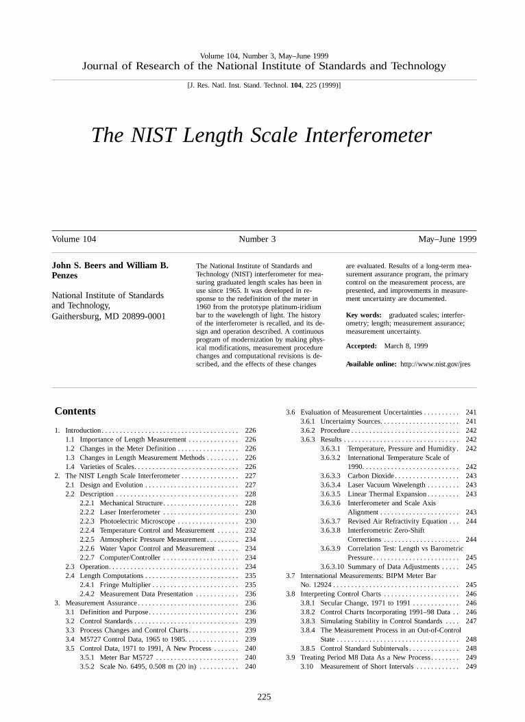
Volume 104, Number 3, May–June 1999 Journal of Research of the National Institute of Standards and Technology [J. Res. Natl. Inst. Stand. Technol. 104, 225 (1999)] The NIST Length Scale Interferometer Volume 104 Number 3 May–June 1999 John S. Beers and William B. Penzes National Institute of Standards and Technology, Gaithersburg, MD 20899-0001 The National Institute of Standards and Technology (NIST) interferometer for mea- suring graduated length scales has been in use since 1965. It was developed in re- sponse to the redefinition of the meter in 1960 from the prototype platinum-iridium bar to the wavelength of light. The history of the interferometer is recalled, and its de- sign and operation described. A continuous program of modernization by making phys- ical modifications, measurement procedure changes and computational revisions is de- scribed, and the effects of these changes are evaluated. Results of a long-term mea- surement assurance program, the primary control on the measurement process, are presented, and improvements in measure- ment uncertainty are documented. Key words: graduated scales; interfer- ometry; length; measurement assurance; measurement uncertainty. Accepted: March 8, 1999 Available online: http://www.nist.gov/jres 3.6 Evaluation of Measurement Uncertainties .......... 241 3.6.1 Uncertainty Sources...................... 241 3.6.2 Procedure .............................. 242 3.6.3 Results ................................ 242 3.6.3.1 Temperature, Pressure and Humidity. 242 3.6.3.2 International Temperature Scale of 1990........................... 242 3.6.3.3 Carbon Dioxide .................. 243 3.6.3.4 Laser Vacuum Wavelength ......... 243 3.6.3.5 Linear Thermal Expansion ......... 243 3.6.3.6 Interferometer and Scale Axis Alignment ...................... 243 3.6.3.7 Revised Air Refractivity Equation . . . 244 3.6.3.8 Interferometric Zero-Shift Corrections ..................... 244 3.6.3.9 Correlation Test: Length vs Barometric Pressure ........................ 245 3.6.3.10 Summary of Data Adjustments ..... 245 3.7 International Measurements: BIPM Meter Bar No. 12924 ................................... 245 3.8 Interpreting Control Charts ..................... 246 3.8.1 Secular Change, 1971 to 1991 ............. 246 3.8.2 Control Charts Incorporating 1991–98 Data . . 246 3.8.3 Simulating Stability in Control Standards .... 247 3.8.4 The Measurement Process in an Out-of-Control State .................................. 248 3.8.5 Control Standard Subintervals .............. 248 3.9 Treating Period M8 Data As a New Process ........ 249 3.10 Measurement of Short Intervals ............ 249 Contents 1. Introduction ...................................... 226 1.1 Importance of Length Measurement .............. 226 1.2 Changes in the Meter Definition ................. 226 1.3 Changes in Length Measurement Methods ......... 226 1.4 Varieties of Scales............................. 226 2. The NIST Length Scale Interferometer ................ 227 2.1 Design and Evolution .......................... 227 2.2 Description .................................. 228 2.2.1 Mechanical Structure ..................... 228 2.2.2 Laser Interferometer ..................... 230 2.2.3 Photoelectric Microscope ................. 230 2.2.4 Temperature Control and Measurement ...... 232 2.2.5 Atmospheric Pressure Measurement ......... 234 2.2.6 Water Vapor Control and Measurement ...... 234 2.2.7 Computer/Controller ..................... 234 2.3 Operation.................................... 234 2.4 Length Computations .......................... 235 2.4.1 Fringe Multiplier ........................ 235 2.4.2 Measurement Data Presentation ............ 236 3. Measurement Assurance ............................ 236 3.1 Definition and Purpose ......................... 236 3.2 Control Standards ............................. 239 3.3 Process Changes and Control Charts .............. 239 3.4 M5727 Control Data, 1965 to 1985............... 239 3.5 Control Data, 1971 to 1991, A New Process ....... 240 3.5.1 Meter Bar M5727 ....................... 240 3.5.2 Scale No. 6495, 0.508 m (20 in) ........... 240 225
Transcript of The NIST Length Scale Interferometer
Volume 104, Number 3, May–June 1999Journal of Research of the National Institute of Standards and Technology
[J. Res. Natl. Inst. Stand. Technol.104, 225 (1999)]
The NIST Length Scale Interferometer
Volume 104 Number 3 May–June 1999
John S. Beers and William B.Penzes
National Institute of Standardsand Technology,Gaithersburg, MD 20899-0001
The National Institute of Standards andTechnology (NIST) interferometer for mea-suring graduated length scales has been inuse since 1965. It was developed in re-sponse to the redefinition of the meter in1960 from the prototype platinum-iridiumbar to the wavelength of light. The historyof the interferometer is recalled, and its de-sign and operation described. A continuousprogram of modernization by making phys-ical modifications, measurement procedurechanges and computational revisions is de-scribed, and the effects of these changes
are evaluated. Results of a long-term mea-surement assurance program, the primarycontrol on the measurement process, arepresented, and improvements in measure-ment uncertainty are documented.
Key words: graduated scales; interfer-ometry; length; measurement assurance;measurement uncertainty.
Accepted: March 8, 1999
Available online: http://www.nist.gov/jres
3.6 Evaluation of Measurement Uncertainties. . . . . . . . . . 2413.6.1 Uncertainty Sources. . . . . . . . . . . . . . . . . . . . . . 2413.6.2 Procedure. . . . . . . . . . . . . . . . . . . . . . . . . . . . . . 2423.6.3 Results. . . . . . . . . . . . . . . . . . . . . . . . . . . . . . . . 242
3.6.3.1 Temperature, Pressure and Humidity . 2423.6.3.2 International Temperature Scale of
1990. . . . . . . . . . . . . . . . . . . . . . . . . . . 2423.6.3.3 Carbon Dioxide. . . . . . . . . . . . . . . . . . 2433.6.3.4 Laser Vacuum Wavelength. . . . . . . . . 2433.6.3.5 Linear Thermal Expansion. . . . . . . . . 2433.6.3.6 Interferometer and Scale Axis
Alignment . . . . . . . . . . . . . . . . . . . . . . 2433.6.3.7 Revised Air Refractivity Equation . . . 2443.6.3.8 Interferometric Zero-Shift
Corrections. . . . . . . . . . . . . . . . . . . . . 2443.6.3.9 Correlation Test: Length vs Barometric
Pressure. . . . . . . . . . . . . . . . . . . . . . . . 2453.6.3.10 Summary of Data Adjustments. . . . . 245
3.7 International Measurements: BIPM Meter BarNo. 12924. . . . . . . . . . . . . . . . . . . . . . . . . . . . . . . . . . . 245
3.8 Interpreting Control Charts. . . . . . . . . . . . . . . . . . . . . 2463.8.1 Secular Change, 1971 to 1991. . . . . . . . . . . . . 2463.8.2 Control Charts Incorporating 1991–98 Data . . 2463.8.3 Simulating Stability in Control Standards. . . . 2473.8.4 The Measurement Process in an Out-of-Control
State. . . . . . . . . . . . . . . . . . . . . . . . . . . . . . . . . . 2483.8.5 Control Standard Subintervals. . . . . . . . . . . . . . 248
3.9 Treating Period M8 Data As a New Process. . . . . . . . 2493.10 Measurement of Short Intervals. . . . . . . . . . . . 249
Contents
1. Introduction. . . . . . . . . . . . . . . . . . . . . . . . . . . . . . . . . . . . . . 2261.1 Importance of Length Measurement. . . . . . . . . . . . . . 2261.2 Changes in the Meter Definition. . . . . . . . . . . . . . . . . 2261.3 Changes in Length Measurement Methods. . . . . . . . . 2261.4 Varieties of Scales. . . . . . . . . . . . . . . . . . . . . . . . . . . . . 226
2. The NIST Length Scale Interferometer. . . . . . . . . . . . . . . . 2272.1 Design and Evolution. . . . . . . . . . . . . . . . . . . . . . . . . . 2272.2 Description. . . . . . . . . . . . . . . . . . . . . . . . . . . . . . . . . . 228
2.2.1 Mechanical Structure. . . . . . . . . . . . . . . . . . . . . 2282.2.2 Laser Interferometer. . . . . . . . . . . . . . . . . . . . . 2302.2.3 Photoelectric Microscope. . . . . . . . . . . . . . . . . 2302.2.4 Temperature Control and Measurement. . . . . . 2322.2.5 Atmospheric Pressure Measurement. . . . . . . . . 2342.2.6 Water Vapor Control and Measurement. . . . . . 2342.2.7 Computer/Controller. . . . . . . . . . . . . . . . . . . . . 234
2.3 Operation. . . . . . . . . . . . . . . . . . . . . . . . . . . . . . . . . . . . 2342.4 Length Computations. . . . . . . . . . . . . . . . . . . . . . . . . . 235
2.4.1 Fringe Multiplier. . . . . . . . . . . . . . . . . . . . . . . . 2352.4.2 Measurement Data Presentation. . . . . . . . . . . . 236
3. Measurement Assurance. . . . . . . . . . . . . . . . . . . . . . . . . . . . 2363.1 Definition and Purpose. . . . . . . . . . . . . . . . . . . . . . . . . 2363.2 Control Standards. . . . . . . . . . . . . . . . . . . . . . . . . . . . . 2393.3 Process Changes and Control Charts. . . . . . . . . . . . . . 2393.4 M5727 Control Data, 1965 to 1985. . . . . . . . . . . . . . . 2393.5 Control Data, 1971 to 1991, A New Process. . . . . . . 240
3.5.1 Meter Bar M5727. . . . . . . . . . . . . . . . . . . . . . . 2403.5.2 Scale No. 6495, 0.508 m (20 in). . . . . . . . . . . 240
225

Volume 104, Number 3, May–June 1999Journal of Research of the National Institute of Standards and Technology
1.3 Changes in Length Measurement Methods
From 1889 to 1960, the international prototypelength standard and the national length standards weregraduated platinum-iridium meter bars. Intercompari-sons of national standards with the prototype bar andcalibrations of all other scales were accomplished incomparators employing filar microscopes for measur-ing length differences between a standard and an un-known [2]. Subinterval lengths were determined in thesame comparators by a lengthy process of intercompari-son by subdivision [3].
In 1958, NIST, then the National Bureau of Stan-dards (NBS), began designing an interferometric linescale comparator in preparation for the proposed changein the definition of the meter. The design was based onthe development of high speed automatic interferencefringe counters in the preceding decade, opening a newera of length measurement by interferometry.
Prior to 1960, wavelengths from selected atomic lightsources were sanctioned by CGPM as secondary real-izations of the meter. These sources were used in mea-suring end standards of length. End standards are bars,usually metal, with optically finished, plane, parallelend faces defining a length. Measured by static interfer-ometry1 since early in the 20th century, their gagingfaces are ideally suited to this method because they canserve as mirrors in the measuring legs of interferome-ters. Line scales cannot be measured efficiently by thestatic method for a number of reasons including themultiplicity of subintervals. They are best measured bydynamic (displacement) interferometry.
1.4 Varieties of Scales
Graduated length scales come in many forms, and aremade in lengths from a few micrometers to over ameter. Those longer than a meter or two are usuallyclassified as measuring tapes or rods. Many materialsare used including steel, Invar, glass, glass-ceramics,silicon, and fused silica. Cross sectional shape can berectangular, “H,” modified “U” (flat bottom), or a mod-ified “X” (Tresca). At present, the line scale interferom-eter is limited to graduation widths ranging from sub-micrometer to 100mm, and spacings ranging from lessthan 1 mm up to 1025 mm. Spacings are generallymeasured from center to center of the graduations, butcan also be measured from edge to edge.
1 A static interferometer is defined as one where none of the opticalcomponents are intended to move during a measurement and theinterference pattern is stationary. A dynamic interferometer is onewhere an optical component, usually a retroreflector, moves and thedisplacement of the moving element is measured by interferencefringe counting or its equivalent.
3.11 Long Term Variability. . . . . . . . . . . . . . . . . . . . 2503.12 Measurement Uncertainty. . . . . . . . . . . . . . . . . . 2503.13 Conclusions. . . . . . . . . . . . . . . . . . . . . . . . . . . . . 250
4. Future Plans. . . . . . . . . . . . . . . . . . . . . . . . . . . . . . . . . . . . . 2514.1 Increase Line Detection Resolution. . . . . . . . . . . . . . . 2514.2 Upgrade the Displacement Interferometers. . . . . . . . . 2514.3 Upgrade the Data Acquisition and Control
Computer System and Their Interfaces. . . . . . . . . . . . 2514.4 Improve the Mechanical Structure. . . . . . . . . . . . . . . . 251
5. Summary. . . . . . . . . . . . . . . . . . . . . . . . . . . . . . . . . . . . . . . . 2516. References. . . . . . . . . . . . . . . . . . . . . . . . . . . . . . . . . . . . . . . 251
1. Introduction
1.1 Importance of Length Measurement
Major changes have occurred in dimensional metrol-ogy in response to rapidly increasing scientific and in-dustrial accuracy requirements over the past severaldecades. Accurate measurements of all kinds are vitallyimportant to many scientific and industrial operations,and measurement of length is fundamental. Measure-ment of physical objects for quality control and processcontrol is part of this picture. Semiconductor manufac-turers, for example, have achieved remarkable improve-ments in quality control on ever smaller circuitry as aresult of improved metrology in mask fabrication andproduction processes. Linear rules in many forms fromencoded scales to photo lithographic grids are oftenused as check standards for such purposes and must becalibrated, when usage requires, to relate them to theinternational standard of length. For more than thirtyyears the evolutionary development and performance ofthe NIST length scale interferometer has influencedimprovement in high accuracy length measurements.
1.2 Changes in the Meter Definition
In 1960 the Confe´rence Ge´nerale des Poids etMesures (CGPM) adopted a new definition of the meterspecifying it as an exact number of vacuum wave-lengths of a particular spectral line of the86Kr isotope.This replaced the prototype platinum-iridium meter barkept at the Bureau International des Poids et Mesures(BIPM) in Sevres, France as the international definitionsince 1889. Again in 1983, the CGPM redefined themeter, this time as the path length traveled by light invacuum in 1/299792458 second [1]. In both redefini-tions great pains were taken to make as little change aspossible in the actual length of the meter. Along withthe 1983 action, the CGPM sanctioned several vacuumwavelengths of iodine stabilized helium neon lasers asworking length standards for relatively short lengths.Time-of-flight measurements are generally impractica-ble for lengths less than 50 m.
226

Volume 104, Number 3, May–June 1999Journal of Research of the National Institute of Standards and Technology
Some devices that are not strictly linear scales aremeasured in the line scale interferometer. These includeend standards in a size range (250 mm to 1000 mm) thatcan present measurement problems with static interfer-ometry. They are converted into line scales with ruledauxiliary blocks wrung to each end [4]. Once converted,the distance between the graduations is measured andthen the auxiliary block line spacing is subtracted toarrive at the length of the end standard. Grid plates aremeasured by treating each row and column of gradua-tions as an independent scale and, when possible, anestimate of orthogonality can be made by measuring thediagonals.
2. The NIST Length Scale Interferometer
2.1 Design and Evolution
By 1961 an experimental Michelson type fringecounting interferometer using a198Hg light source as alength standard was tested [5], but restricted coherence
in atomic sources limited the range to about a decime-ter. Development of a final version capable of measur-ing length scales proceeded, by good fortune, in parallelwith the development of lasers [6]. The remarkablecoherence of laser light made it ideal for fringe countinginterferometry over long distances. In 1965, the twoactivities converged and a successful measurement of a1 m scale with helium-neon laser wavelengths wasaccomplished [7]. Further refinements were then madein the line scale interferometer and laser wavelengthstability was improved. By 1966, a semi-automatedlength scale measurement system was in operation [8].The mechanical and optical structures as they existed atthat time are shown in Fig. 1.
Development has continued on both the line scaleinterferometer [9] and on lasers [10, 11]. The majorchanges were: (1) rigid coupling and kinematic mount-ing of the microscope and interferometer fixed leg in1970, (2) replacement of the Michelson-type planemirror interferometer with a commercial laser interfer-
Fig. 1. The length scale interferometer mechanical and optical components prior to 1970.
227

Volume 104, Number 3, May–June 1999Journal of Research of the National Institute of Standards and Technology
ometer in 1979, (3) modernization of the microscopeelectronics together with the addition of a computer/controller in 1981 to completely modernize and auto-mate the instrument [12].
Many minor modifications in the mechanical struc-ture were also made as well as important changes inmeasurement procedures, data processing, and compu-tational methods. These will be discussed under mea-surement assurance (Sec. 3).
2.2 Description
The major components of the instrument are:1. A 2 m waybed with a lead-screw driven carriage
for translating the scale.2. A fixed position photoelectric microscope with a
servo system for centering scale graduations in themicroscope field.
3. An interferometer using a stabilized laser lightsource as a length standard for measuring scales.
4. Measuring devices for temperature, barometricpressure, and air moisture content for use in com-puting laser wavelengths at ambient conditions.
5. A computer/controller for data recording and pro-cessing, and for automated instrument operation.
6. A temperature controlled enclosure to provide astable environment for the instrument.
2.2.1 Mechanical Structure
The 2 m waybed and its main carriage, originally alinear dividing engine made by the Socie´te Genevoised’Instruments de Physique (SIP)
2, was modified at NBS
for use as the mechanical foundation of the length scaleinterferometer. The main carriage has precision rollerbearing wheels and rides on hand scraped guide ways. Itis moved by a 1 mmpitch, 1025 mm long, lead screw.
Since modification, the main carriage is coupled tothe lead screw by a nylon half-nut and the screw isdriven by a computer controlled stepping motor forcoarse scale positioning. The weighted half-nut rides ontop of the screw to permit easy decoupling for manuallyand quickly moving the carriage back and forth duringscale and interferometer alignment procedures.
As shown in Figs. 2a and 2b, a superstructure ismounted atop the main carriage to provide a scalemounting platform. Mechanical controls for focusingand aligning the scale, and a servo actuator for centeringscale graduations in the microscope field, are also
2 Certain commercial equipment, instruments, or materials are identi-fied in this paper to foster understanding. Such identification does notimply recommendation or endorsement by the National Institute ofStandards and Technology, nor does it imply that the materials orequipment identified are necessarily the best available for thepurpose.
provided. Line centering is accomplished by a servosignal from the photoelectric microscope to a pair ofhydraulic pressure actuators, one on each side of thesuperstructure. Pressure is applied to flexure plates thatsupport the superstructure at the right end. A pair ofcables suspend the structure at the left end so it is freeto move several micrometers along its axis as pressureis applied in the line centering process.
The scale mounting platform is a 110 cm35 cm3 0.95 cm Invar plate with a retroreflectorattached to each end, serving as the moving elements intwo separately or simultaneously operating interferom-eter systems. Each system has its own laser and counter.A fixed position remote interferometer, consisting of abeam splitter and a cube corner retroreflector in a com-pact assembly, is located near each end of the waybed.Each remote interferometer splits its laser beam intotwo beams of equal intensity. One beam forms a refer-ence leg within the contiguous retroreflector, and theother forms a measuring leg with the moveable retrore-flector.
One remote interferometer and the microscope areattached to opposite ends of a 1075 mm rigid steel tubeand this assembly is mounted over the waybed on athree point kinematic support. The right end of theassembly (with its remote interferometer) is fixed to thewaybed. The left end (with the microscope) is near thewaybed midpoint. It rests on a ball between two flats onthe far side of the waybed and a ball between a flat anda “V” groove parallel to the ways on the near side. Asecond remote interferometer is at the extreme left onan extension of the steel tube. If the microscope andinterferometers were rigidly and independently attachedto the waybed, they would be shifted by the heavycarriage as it moves on the waybed. Rigid interconnec-tion and kinematic mounting of these components freesthem from this shifting.
It is vital that the distance between the microscopeand the remote interferometers remains fixed during ascale measurement because any relative motionbetween them will be seen as part of the measured scalelength, thus obviously resulting in uncertainties. By thesame token, it is vital that the dimension between thescale and the retroreflectors remain fixed during a mea-surement.
The entire apparatus is housed in a vibration isolatedand thermally insulated enclosure held at 208C by athermostatically controlled circulating water system. Aplywood box forms the outside of the enclosure. It islined with plastic foam insulation and a sheet copperinner lining having copper tubing soldered to it forcarrying the thermostated water. The upper half of theenclosure consists of three raisable sections providingaccess to the instrument.
228

Volume 104, Number 3, May–June 1999Journal of Research of the National Institute of Standards and Technology
229
– –
Fig
.2a.
Pho
togr
aph
ofth
ele
ngth
scal
ein
terf
erom
eter
inits
pres
ent
form
.
Fig
.2b.
Sch
emat
icdi
agra
mof
the
leng
thsc
ale
inte
rfer
omet
erin
itspr
esen
tfo
rm.

Volume 104, Number 3, May–June 1999Journal of Research of the National Institute of Standards and Technology
2.2.2 Laser Interferometer
A Michelson-type, plane mirror interferometer wasused in the instrument until 1979. It was replaced witha Hewlett-Packard (HP) model 5526A He-Ne laser in-terferometer. Elements of the HP interferometer areshown in Fig. 3. It can be readily integrated into anautomated, computer controlled system. Aligning theoptical components is much simpler with the HP system.However, the ability was lost to compensate for wavi-ness and deviations in straightness of the ways providedin the Michelson by a servo system [12] that kept theoptical flats parallel to each other as the carriage moved.To minimize sine and cosine measurement uncertaintiesintroduced by carriage pitch (from waviness) and yaw(from straightness deviations), the optical axis of the HPinterferometer is always aligned in coincidence with thescale graduation axis.
2.2.3 Photoelectric Microscope
Line scales are calibrated by making carriage dis-placement, as measured by the interferometer, corre-spond exactly to scale interval lengths. The key to thiscorrespondence is the line centering action of the pho-toelectric microscope that occurs when the carriage isstopped and a graduation is in view. This process isdescribed below.
The high speed stepping motor and its indexer areinterfaced with the system computer/controller to movethe carriage predetermined distances corresponding tonominal line spacings on the scale. During final index-ing steps for each interval the stepping motor goes intoa slow mode and actuates microscope electronics thattrigger a stop-motor signal when the line appears in themicroscope field. Once the carriage is stopped, line cen-tering electronic circuits take over. The graduation isthen centered in the field by means of electro-hydraulicactuators on the scale support structure. Therefore,starting at the zero graduation, and ending at the termi-nal graduation, the interferometer measures the dis-tances from line center to line center of pre-selectedintervals, thus calibrating the scale. In actual use, severalpasses are made up and down the scale to obtain redun-dancy needed for averaging and statistical analysis.
In both design and operation the photoelectric micro-scope is the most complex part of the length scale inter-ferometer. A schematic diagram of the microscopeoptics is shown in Fig. 4. An oscillating mirror sweepsa magnified image of the vertically illuminated scalegraduation segment across a slit in front of a photomultiplier. A sinusoidal scanning mode is used ratherthan a linear mode to avoid all the harmonics of thescanning frequency. The torsional-pendulum scannerhas a very high vibrational Q of 1000 and has a resonantfrequency of 70 Hz. Since the scan has only one fre-quency, and the scanner is mechanically resonant, itscenter of oscillation is very reliable and has a close andfixed relation to the microscope optical center. This isextremely important to microscope operation becausethe line center is locked to the oscillation center wheninterferometer readings are made, and the oscillationcenter is the operational center of the microscope field.
Scale graduations are of two types as seen by themicroscope: bright (reflective) lines against a darkbackground, or dark lines against a bright background.Graduation images are produced with the aid of a mi-croscope illuminator which projects a uniformly litbeam of light through the objective lens and normal tothe scale surface. If graduations are chrome on a trans-parent substrate the line will reflect light and appearbright on a dark background. The reverse of this willappear if the background is chrome and the line is
Fig. 3. The Hewlett-Packard interferometer system.
The Michelson and the HP system were operatedsimultaneously from opposite ends of the waybed dur-ing a transition period to verify comparability. An iodinestabilized He-Ne laser was used with the Michelsonduring periods in 1976 and 1978 to confirm wavelengthvalues of the Lamb-dip stabilized He-Ne laser in use atthe time. Short term fractional stability of the HP laserwavelength was 13 10–8, and long term fractionalstability was 13 10–7. Long term fractional stability ofthe iodine stabilized laser was 13 10–10.
The HP interferometer is operated in a 1/4 wavelengthcounting mode with interpolation between counts. Mea-sured values of air temperature, barometric pressure,relative humidity, and CO2 content are used to calculatethe refractive index of air in the interferometer path.Ambient wavelength is then derived from the NIST-calibrated vacuum wavelength and the refractive index tomake scale length computations.
230

Volume 104, Number 3, May–June 1999Journal of Research of the National Institute of Standards and Technology
Fig. 4. Scanning photoelectric microscope schematic diagram.
transparent. On a metal scale the surface is flat andhighly polished, and the lines are cut into the metal witha diamond ruling point producing a dark line on a brightbackground. The line appears black because the illumi-nating light is scattered by the sloped sides of the V-shaped groove cut by the ruling point. Some ruled linesare partially filled with printers ink to enhance theirdarkness and avoid reflections from the flat bottom ofthe groove. High quality lines are uniform in width andhave smooth sharp edges. Typically, they come inwidths from 1mm to 10mm.
Several electronic circuits are employed in operatingthe microscope. These are a mirror drive oscillator,optical signal processor, line center deviation detector,indexer control interface, and a proportional plus inte-gral servo driver. The line signal derived from the photomultiplier is displayed on an oscilloscope operating inthe x–y plot mode. The horizontal input of the scope,representing the scan, is driven by the sinusoidal signalfrom the mirror drive oscillator circuit, while the verti-cal axis represents light level. Thus, a linear signal isdisplayed on the screen showing the line profile and itsposition relative to the scan (microscope) center.
Optical signal processor and line center deviationdetector circuits transform the signal into a means forline centering. A pair of positive and negative peakdetectors make up the optical signal processor. The
difference between positive and negative peak voltagesrepresents the deviation of the line center from the scancenter. A threshold voltage derived from the scaledamplitude of the line signal is displayed on the oscillo-scope as a horizontal line intersecting the line signalpattern (see Fig. 5) and is used in the line signal devia-tion detector to produce a dc signal proportional to thedistance of the line center from the scan center. The signof this signal shows the direction of the line from center.Threshold voltage is adjusted with a potentiometer to anoptimum level, usually 50 % of the amplitude, for trig-gering the centering-deviation detector. Using the twopoints where the threshold voltage intersects the linesignal, the line centering deviation detector generates abipolar dc voltage corresponding to the direction, andproportional to the distance, of the line from center.This voltage is used as a correction signal to run theproportional plus integral servo driver which thenmoves the scale support structure (with retroreflectorattached) by electro-hydraulic means to center the line.This servo system loop will continuously and dynami-cally lock a line center onto the scan center of themicroscope field. Centering of a line edge can beachieved using the intersection of the threshold withone edge or the other of the line signal, a useful featurefor special measurements where edge to edge ratherthan center to center measurements are required.
231

Volume 104, Number 3, May–June 1999Journal of Research of the National Institute of Standards and Technology
Fig. 5. Microscope line signal pattern.
From the preceding description it is clear that themicroscope is an edge detector and when it sees bothedges of a line at the same time it will find and use itscenter. Although this “two point criterion” for determin-ing line centers was chosen for operational reasons, it isremarkably similar in function and result to the bi-filareyepieces used in microscopes employed in traditionalline scale metrology. Thebi-filar microscope has a pairof parallel hairs in the eyepiece assembly slightly fartherapart than the width of the graduation image. Thesehairs are moveable in unison and their position acrossthe field of view is readable by a micrometer screw witha graduated drum and a drum revolution counter. Whenviewing a scale, the line center is located by straddlingthe line with the double hairs and moving them until theopen areas on each side of the line between the lineedges and the hairs are equal. This process takes advan-tage of a human vision characteristic called hyperacuitywhich permits the balancing of areas much moreprecisely than would seem theoretically possible fromthe often erroneously applied criterion of lens resolvingpower. With the hyperacuity phenomenon line centerscan be located in a bi-filar microscope, with a standarddeviation of 40 nm. However, the photoelectric micro-scope can locate line centers to better than a 2 nmstandard deviation.
2.2.4 Temperature Control and Measurement
By international agreement precision length measure-ments are made near, and corrected to, a temperature of20 8C.
The line scale laboratory is in a below-grade room tohelp isolate it from vibration and outdoor temperature
fluctuations. Laboratory temperature is controlled at20 8C 6 0.058C by a thermostated forced air heating/cooling system. Tempered air is distributed evenlythrough a plenum formed by a dropped and perforatedfalse ceiling. Air exits at baseboard level and returnsthrough hollow walls and ducts to the tempering system.
The interferometer enclosure is independently andprecisely temperature controlled to provide the environ-ment needed for accurate length measurements. Figure6 is a schematic diagram of the temperature control andmeasuring system for the interferometer enclosure.Distilled water in a reservoir is cooled at a constant rateby a heat exchanger carrying chilled water at 148C. Asubmerged electric heater proportionally heats thedistilled water to keep it at the 208C set point. A pumpcirculates the water through copper tubing behind thecopper lining of the housing.
When the temperature system is activated for makinga length measurement an error signal comes from athermocouple in the interferometer air path to give pre-cise control at 208C 6 0.0058C, but when the tempera-ture system is not activated the error signal comes froma thermistor in the water line to keep the temperaturenominally correct when the instrument is not in use.
An 0.5 m diameter fan is located on the enclosurebottom to circulate air and reduce temperature gradi-ents. All heat producing elements such as the laser,microscope illuminating lamp, lead screw drive motor,fan motor, and electronic circuits are externallymounted.
At the heart of the temperature control and measure-ment system is a 208C reference temperature cell and acalibrated standard platinum resistance thermometer(SPRT). A schematic of the system is shown in Fig. 7.
232

Volume 104, Number 3, May–June 1999Journal of Research of the National Institute of Standards and Technology
Fig. 6. Temperature control system schematic diagram.
Fig. 7. Reference temperature measuring and control system schematic diagram.
233

Volume 104, Number 3, May–June 1999Journal of Research of the National Institute of Standards and Technology
The cell provides a precise 208C 6 0.00058C referencefor the thermocouples in the temperature measuringsystem. Cell operation is based on the same principles asthe other control systems. It has a constant source ofcooling, provided in this case by a thermoelectriccooler, modulated by feedback to an electric heater tokeep a constant temperature.
Cell temperature is monitored with the SPRT bykeeping the Mueller-type bridge set at the 20.0008Cresistance value. There is some drift in the reference cellheater current controller, but a manual adjustment to thecontrol circuit potentiometer once a day keeps the celltemperature stable to better than 10–3 K.
There are 10 copper-constant thermocouple junctionsinside the enclosure, with their reference junction at-tached to the SPRT in the reference cell. Two are in theinterferometer air path, three are on the scale beingmeasured, and the rest are in various locations wherethey are used to detect gradients and temperature varia-tions. A motor-driven selector switch allows tempera-tures to be read sequentially and displayed in degreesCelsius on a strip chart recorder. There are two operat-ing modes for the system: control and measurement. Inthe control mode the selector switch is locked on onethermocouple in the interferometer air path. Its voltageindicates the deviation from 208C and is the error signalthat feeds back to the water bath temperature control tocorrect the air temperature. The measurement mode isused periodically during a scale measurement by un-locking the selector switch to read air path and scaletemperatures for use in computing scale length.
This system has several advantages. Thermocouplesare very stable and are free from self heating. Thermo-couple voltage measurement uncertainties are mini-mized because the measuring junctions are at nearly thesame temperature as the reference junction making ther-mocouple voltages very small and therefore measurableto high accuracy. In addition, the SPRT and the Muellerbridge are quite stable and do not require frequent cali-bration. Finally, the system is directly traceable throughthe SPRT to the International Temperature Scale of1990 (ITS-90).
2.2.5 Atmospheric Pressure Measurement
Barometric readings are taken with electro-mechani-cal pressure transducers having a sealed chamber with alow stress diaphragm on one wall. As the diaphragmmoves with changes in atmospheric pressure, its posi-tion is detected with a capacitance probe that producesa voltage proportional to pressure. Two barometers ofdifferent manufacture are constantly checked againsteach other to detect drift that may indicate a need for
recalibration. NIST calibrations establish the exact rela-tionship between pressure and voltage.
2.2.6 Water Vapor Control and Measurement
To reduce the possibility of rust forming on steelsurfaces, laboratory relative humidity is held below50 % by the air conditioning system. Water vapor con-tent of the air in the interferometer housing is measuredwith a NIST calibrated, chilled mirror type, dew pointhygrometer. A second similar hygrometer serves as acheck on the primary instrument. An instrument basedon capacitance change in a thin polymer film as itabsorbs or evaporates water from the air provides a thirdreliability check.
2.2.7 Computer/Controller
A Hewlett-Packard desktop computer controls theoperation of the line scale interferometer system. It takesoperator instructions, controls the carriage-drivingstepping motor, records line scale measurement data,computes scale interval lengths, and prints a calibrationreport table complete with statistical analysis andmeasurement uncertainties.
Figure 8 is a schematic diagram of the computer andits interfaces. There are two 16 bit I/O interfaces: onecontrols the stepping motor and the other controls theline centering process. The laser interferometer displayunit is connected to the BCD interface to receive quarterwavelength counts and the interpolated fractional count.
Several instruments are connected to the HP-IB inter-face. A digital voltmeter (DVM) measures the linecentering servo current, a second DVM measures theoutput from a hygrometer, and a third measures theoutput from a barometer. A nanovoltmeter measures thethermocouple outputs to give air and scale temperatures.
2.3 Operation
A scale to be measured is first mounted on the car-riage with its zero graduation at the left (called normalscale orientation). As the carriage is manually movedback and forth the scale is aligned and focussed relativeto the microscope, then the interferometer is alignedcoincident with the scale graduation axis. At the end ofthis procedure the carriage is positioned so the zeroscale graduation is in the microscope field. After thetemperature stabilizes at or very near 208C, and temper-ature gradients are minimized (usually overnight), thescale is ready for measurement. A computer programgoverns the measurement process. Preliminary data thatmust be entered by the computer operator includes scale
234

Volume 104, Number 3, May–June 1999Journal of Research of the National Institute of Standards and Technology
Fig. 8. Computer interfaces for the length scale measuring system.
identification, scale thermal expansion coefficient, datafile name, the intervals to be measured, and the numberof measurement passes to be made. Interferometer pathair temperature and relative humidity, scale temperature,and barometric pressure can be entered by the operatoror read automatically. Although set to a nominal zero atthis point, the interferometer always displays a fractionalcount which is read by the computer at the start of themeasurement.
The computer starts the measuring process as soon aspreliminary data are entered. It verifies that a graduationis present and centered in the photoelectric microscopefield, and reads the initial interferometer count. It alsocalculates the steps required of the stepping motor toreach a point just short of the next programmed gradua-tion, and starts the stepping motor in its high speedmode. When the required steps are reached the motorshifts into its low speed mode and the microscope elec-tronic circuits are activated. As the graduation enters themicroscope field the line detection circuit stops the step-ping motor and activates the hydraulic line centeringservo system. When the line is centered, the interferom-eter is read. This process is repeated for each succeedingequally spaced graduation until the terminal graduationis reached. The operator enters a reduced list of prelim-inary data for the return pass and the process reversesuntil it closes at the zero graduation. More passes areperformed as needed.
The scale is then remounted on the carriage with thezero graduation at the right end (reversed orientation),and the process is repeated as for the normal orientation.
Two passes in each orientation is the minimum toprovide valid statistical information. Increasing thenumber of passes generally reduces standard deviationand, consequently, uncertainty.
2.4 Length Computations
Data from the measuring system is converted intoscale interval lengths at 208C by the computer program.The count recorded at the zero graduation is subtractedfrom each succeeding recorded count in the pass to givethe interval lengths in quarter wavelength units. A fringemultiplier then converts these into scale length units at20 8C.
2.4.1 Fringe Multiplier
Three elements are combined in the fringe multiplier:(1) laser vacuum wavelength,l0, (2) refractive index ofambient air in the interferometer,ntpf, and (3) scale ex-pansion,DL from observed temperature to 208C. Laservacuum wavelength is determined by NIST calibration.
Until 1991 the refractive index of air was computedfrom Edlen 1966 equation [13]. Birch and Downs [14]recently developed a modified form of the equation thatprovides significant improvement in uncertainty [15].The changes are mainly in the correction for airmoisture and in values for CO2 content of air. A massfraction value of 3003 10–6 of CO2 is used in theoriginal Edlen equation. Birch and Downs use4503 10–6 as typical of their laboratory air, but in the
235
Volume 104, Number 3, May–June 1999Journal of Research of the National Institute of Standards and Technology
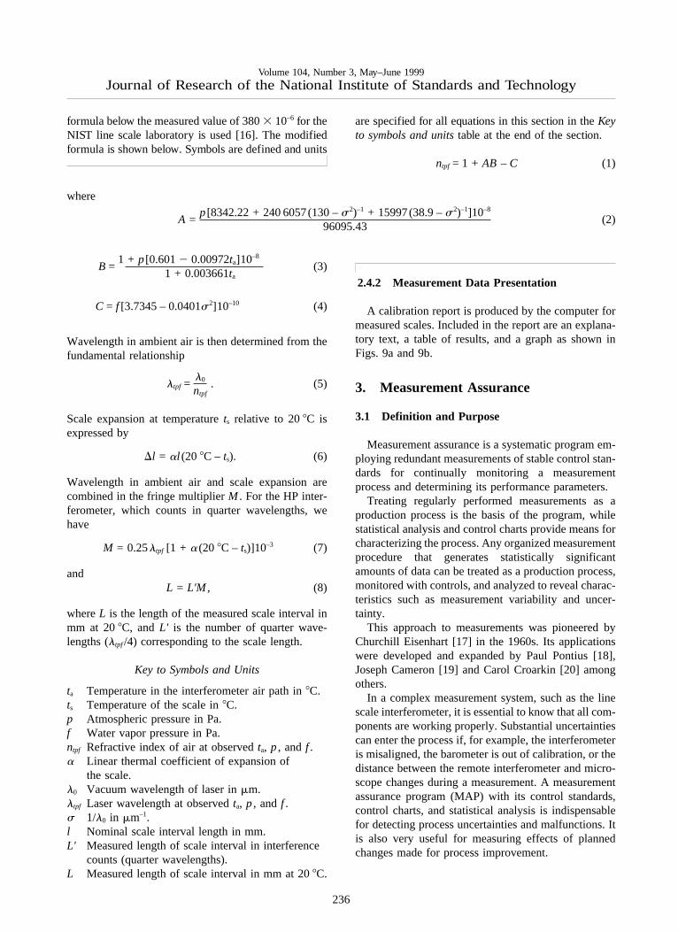
formula below the measured value of 3803 10–6 for theNIST line scale laboratory is used [16]. The modifiedformula is shown below. Symbols are defined and units
are specified for all equations in this section in theKeyto symbols and unitstable at the end of the section.
ntpf = 1 + AB – C (1)
where
A =p[8342.22 + 240 6057(130 –s2)–1 + 15997(38.9 –s2)–1]10–8
96095.43(2)
B =1 + p[0.6012 0.00972ta]10–8
1 + 0.003661ta(3)
C = f [3.7345 – 0.0401s2]10–10 (4)
Wavelength in ambient air is then determined from thefundamental relationship
ltpf =l0
ntpf. (5)
Scale expansion at temperaturets relative to 208C isexpressed by
Dl = al (20 8C – ts). (6)
Wavelength in ambient air and scale expansion arecombined in the fringe multiplierM . For the HP inter-ferometer, which counts in quarter wavelengths, wehave
M = 0.25ltpf [1 + a (20 8C – ts)]10–3 (7)
andL = L'M , (8)
whereL is the length of the measured scale interval inmm at 208C, andL' is the number of quarter wave-lengths (ltpf/4) corresponding to the scale length.
Key to Symbols and Units
ta Temperature in the interferometer air path in8C.ts Temperature of the scale in8C.p Atmospheric pressure in Pa.f Water vapor pressure in Pa.ntpf Refractive index of air at observedta, p, andf .a Linear thermal coefficient of expansion of
the scale.l0 Vacuum wavelength of laser inmm.ltpf Laser wavelength at observedta, p, andf .s 1/l0 in mm–1.l Nominal scale interval length in mm.L' Measured length of scale interval in interference
counts (quarter wavelengths).L Measured length of scale interval in mm at 208C.
2.4.2 Measurement Data Presentation
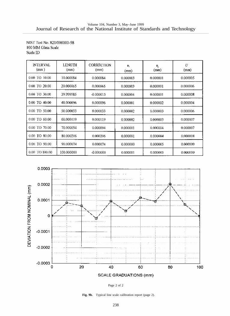
A calibration report is produced by the computer formeasured scales. Included in the report are an explana-tory text, a table of results, and a graph as shown inFigs. 9a and 9b.
3. Measurement Assurance
3.1 Definition and Purpose
Measurement assurance is a systematic program em-ploying redundant measurements of stable control stan-dards for continually monitoring a measurementprocess and determining its performance parameters.
Treating regularly performed measurements as aproduction process is the basis of the program, whilestatistical analysis and control charts provide means forcharacterizing the process. Any organized measurementprocedure that generates statistically significantamounts of data can be treated as a production process,monitored with controls, and analyzed to reveal charac-teristics such as measurement variability and uncer-tainty.
This approach to measurements was pioneered byChurchill Eisenhart [17] in the 1960s. Its applicationswere developed and expanded by Paul Pontius [18],Joseph Cameron [19] and Carol Croarkin [20] amongothers.
In a complex measurement system, such as the linescale interferometer, it is essential to know that all com-ponents are working properly. Substantial uncertaintiescan enter the process if, for example, the interferometeris misaligned, the barometer is out of calibration, or thedistance between the remote interferometer and micro-scope changes during a measurement. A measurementassurance program (MAP) with its control standards,control charts, and statistical analysis is indispensablefor detecting process uncertainties and malfunctions. Itis also very useful for measuring effects of plannedchanges made for process improvement.
236

Volume 104, Number 3, May–June 1999Journal of Research of the National Institute of Standards and Technology
Fig. 9a. Typical line scale calibration report (page 1).
237
Volume 104, Number 3, May–June 1999Journal of Research of the National Institute of Standards and Technology
Page 2 of 2
Fig. 9b. Typical line scale calibration report (page 2).
238

Volume 104, Number 3, May–June 1999Journal of Research of the National Institute of Standards and Technology
3.2 Control Standards
Two primary control standards are used to monitorthis process. The first control, introduced in 1966, is aSIP Invar meter bar, M5727. It has an H shaped crosssection with its neutral plane, located on the upper sur-face of the H cross piece, graduated in millimeters. Thesecond control, introduced in 1982, is an 0.508 m(20 in) steel scale, No. 6495, graduated each 1.27 mm(0.05 in). A measurement process such as this one,which runs for decades, should have dimensionallystable control standards but completely stable materialsare very rare, perhaps even non-existent. This can makeit difficult to distinguish real from apparent secularlength changes in the controls.
3.3 Process Changes and Control Charts
Figure 10 is the control chart showing the measure-ment history of M5727 (0 m to 1 m interval) from 1965to 1985. Individual measurement values are plotted. Achange in the measurement process was made at eachvertical line, dividing the plot into periods. The meanvalue for each period is shown as a horizontal solid line,and the limits shown with dotted lines are6 3s wheres is the standard deviation of a single value.3 The6 3scontrol limits are used to judge individual measure-ments. They are a statistical prediction, based on pastperformance, that 99.7 % of future measured values willfall within them. Values falling outside these controllimits are judged to result from an out-of-control condi-tion and require an investigation into the cause and acorrection of the fault. The 3s level is a generallyaccepted value for judging performance in measurementassurance programs.
Each process change and the mean value for its periodis designated by M1 through M4. The change associatedwith each mean is described in Table 1. Data taken andchanges made after 1985, designated as M5 throughM8, are also described in the table but will be dealt withlater in the text.
An individual measurement is defined here as themean of two data sets of two passes each. One set istaken with the bar in the normal orientation (zero grad-uation at the left) and consists of one pass up the scalefrom zero to the terminal graduation (one meter in thiscase), and one pass down the scale, closing at the zerograduation. Data stops are made at each decimeter inboth directions. The second set consists of two passestaken in a similar manner but with the bar in thereversed orientation (zero graduation at the right).
Two critical interferometer dimensions are givenspecial attention in making process changes. These are:
3 These conventions will be followed throughout for control charts.
(1) distance between microscope and interferometerbeam splitter, and (2) distance between retroreflectorand scale. Changes in these relationships during a scalemeasurement will cause uncertainties.
Fig. 10. Meter M5727 control chart, 0 m to 1 m,1971 to 1991.
Table 1. Sequence and descriptions of process changes
Periodsymbol Period descriptions
M1 Mean of data from classical meter bar intercomparisons (indi-vidual points not shown).
M2 Data from the first interferometric measurements.M3 Data taken after the microscope, beam splitter and reference
mirror were rigidly coupled forming an assembly that was kine-matically mounted on the waybed. This change was designed toreduce the effect of the heavy moving carriage on the criticaldimension between microscope and beamsplitter.
M4 Data taken after replacing the original Michelson type interfer-ometer with a commercial laser interferometer system mountedat the opposite end of the waybed. No carriage pitch or yawcorrections were made after this change, but scales are nowmounted with their ruled axes coincident with the interferome-ter axis to eliminate Abbe´ offset and its attendant uncertainties.
M5 Data taken after the interferometer retroreflector was movedfrom its mount on the subcarriage to a mount on the scalesupport structure (see Fig. 2). This reduced the possibility ofchange, during a scale measurement, in the critical distancebetween scale and retroreflector.
M6 Data taken after recalibrating the barometer and temperaturesystem, and replacing the hygrometer.
M7 Data taken after the retroreflector was mounted on a new Invarscale support structure to further reduce chances of a criticaldistance change. Zero-shift (deadpath) corrections were appliedduring this and subsequent periods.
M8 Data taken after incorporating a modified version of Edle´n’srefractive index equation into the process and mounting ahygrometer inside the interferometer housing.
3.4 M5727 Control Data, 1965 to 1985
Table 2 shows the mean value and long term mea-surement variability, as represented by control chartlimits, for each period shown graphically in Fig. 10.
239

Volume 104, Number 3, May–June 1999Journal of Research of the National Institute of Standards and Technology
and more precise than with the Michelson, and the re-sulting improved measurement variability can be seenin period M4.
In the 1986 evaluation [20] of M1 through M4 data,a possibility of real secular lengthening of M5727, assuggested by the slope of a fitted line, was considered.It was rejected for several reasons. Most important wasthat the first interferometric measurement period, M2,was the least reliable, having been taken before thefixed optical components of the interferometer and themicroscope were rigidly coupled and kinematicallymounted. The change in mean value from M2 to M3was, therefore, discounted as evidence for dimensionalchange in M5727. The relatively small change inM5727 from M3 to M4 was not statistically significant,but it might be attributable to measurement processchange M4 (replacement of the Michelson type with anHP interferometer). However, the two interferometerswere operated simultaneously, from opposite ends ofthe waybed, for a short period in 1979 to verify continu-ity. They agreed to within 0.01mm in the measurementof M5727.
3.5 Control Data, 1971 to 1991, A New Process
3.5.1 Meter Bar M5727
Figure 11 shows M5727 measurement history to1991 with M1 and M2 data deleted to eliminate influ-ence from biased early data. Starting with period M3 thedata are treated as a new process reflecting major struc-tural and operational changes that produced improve-ments in measurement results. Vertical lines correspondto process changes M5 through M7 in Table 1 (M8 datawill be shown and discussed later). Horizontal lines areperiod mean values. This additional data strengthens thecase for a gradual lengthening of this bar.
3.5.2 Scale No. 6495, 508 mm (20 inches)
Figure 12 is the history of steel control bar No. 6495plotted on the same time scale as meter bar M5727 in
Table 2. Mean value and control chart limits for periods M1 throughM4
Mean Control chart limitsPeriod value 6 3s
(mm) (mm)
M1 1.33 0.24M2 1.10 0.23M3 1.32 0.16M4 1.37 0.07
The M1 period measurements were made in 1964–65by comparing M5727 with NBS laboratory referencemeter bars in a comparator employing micrometer mi-croscopes to measure the length differences betweenreference bar and unknown in the traditional way [2, 3].The mean value is plotted in Fig. 10 with its 3s controllimits. The first interferometric measurement period,M2, extended from 1966 to 1971. The M2 mean agreedwith M1 within 0.2mm. This was considered to be goodagreement for that time when uncertainties for lengthsup to 1 m were in the range of 0.2mm to 0.5mm.
A major structural change in the interferometer wascompleted in 1971. The photoelectric microscope wasoriginally attached to the side of the waybed at themidpoint, and the beamsplitter was attached to thewaybed at one end (see Fig. 1). A steel I-bar (not shownin Fig. 1) extending from the microscope to the top ofthe beamsplitter assembly was installed very early toconnect more rigidly these two components when itbecame apparent that the microscope angle changedwhen the carriage moved on the ways. The beamreduced this distortion, but a more effective structurewas designed and installed in 1970–71.
In this new structure the microscope and beamsplitterare mounted at opposite ends of a 1 msteel tube and theassembly kinematically mounted on the waybed. Thebeamsplitter end is fixed to the end of the waybed andthe microscope end is supported on two 25.4 mm ballbearings free to roll only in a direction parallel to theways (see Fig. 2). This decoupled the assembly fromwaybed distortions. Period M3 shows resulting mea-surements. There was an improvement in variabilityand a change in apparent length.
By 1978 the original fringe counting and microscopeelectronics were failing from age. In 1979 the electron-ics were replaced with modern components and theoriginal NBS-made, Michelson-type, interferometerwas replaced with a commercial model. All this wasdone while preserving the principles of the originalNBS design. Commercial laser interferometers were bythen quite reliable so a Hewlett-Packard (HP) modelwas installed. HP interferometer alignment was easier Fig. 11. Meter M5727 control chart, 0 m to 1 m,1971 to 1991.
240

Volume 104, Number 3, May–June 1999Journal of Research of the National Institute of Standards and Technology
Fig. 11. During the time common to both scales, thelength of the former appears to be increasing and thelatter appears to be decreasing.
3.6 Evaluation of Measurement Uncertainties
The 1986 uncertainty evaluation (see column labeledProcess relative standard uncertainty, 1986 in Table 3)was based on data up to 1985. In 1987, a re-evaluationof measurement process uncertainties was undertaken.Although control standards are indispensable toolsfor monitoring the measurement process, they have thedisadvantage of undergoing long-term length changes,leaving some doubt about process performance. Conse-quently, three goals were set for the new uncertaintystudy: (1) reduce measurement uncertainties, (2) estab-lish a new measurement uncertainty value by approvedmethods [21], and (3) determine rates and directions ofcontrol bar length changes.
3.6.1 Uncertainty Sources
The following is a list of potential length scale mea-surement process uncertainty sources:
• Wavelength1. Vacuum wavelength of the laser2. Refractive index of air determination
a. Refractive index equationb. Air temperature measurementc. Atmospheric pressure measurementd. Humidity measuremente. Air composition
• Interferometer1. Alignment of interferometer axis with scale
graduation axis (i.e., Abbe offset)2. Structural characteristics
a. Constancy of distance between referencemirror and microscope
b. Constancy of distance between beam splitterand microscope
c. Constancy of distance between measuringretroreflector and scale
• Scale1. Temperature measurement2. Thermal expansion coefficient3. Graduation quality
Except for interferometer structural characteristics,and scale graduation quality, these parameters lead touncertainties proportional to the scale length being mea-sured.
Relative effects of length-dependent uncertainties areillustrated in Table 3 where it is shown, for example,that a 0.1mm length measurement uncertainty will
Fig. 12. Control chart for bar No. 6495, 0 m to 0.508 m, 1982 to1991, plotted on same time scale as Fig. 11.
Table 3. Relationship between length-dependent standard uncertainties and standard uncertainties in measure-ment parameters and estimated process standard uncertainty
Process relativeRelative standard uncertainty standard uncert.
in a 1 mlength 0.01m/mParameter for 0.1mm/m for 0.01mm/m 1986 1994
WavelengthVacuum wavelength 13 10–7 1 3 10–8 5 2Refract. index eq. 13 10–7 1 3 10–8 5 2Air temp. 0.18C 0.018C 0 0Pressure 40 Pa 4 Pa 4 2Rel. humidity 12 % rh 1.2 % rh 3 1CO2 content 673 10–6 2 1
InterferometerAlignment 0.45 mm/m 0.14 mm/m 2 2
ScaleSteel temp. 0.0098C 0.0018C 2 2Glass temp. 0.0128C 0.0018CInvar temp. 0.0678C 0.0078CQuartz temp. 0.2508C 0.0258C
us = 9 5
241

Volume 104, Number 3, May–June 1999Journal of Research of the National Institute of Standards and Technology
result from an uncertainty of 0.0098C in temperaturemeasurement of a one meter steel scale (assuming alinear thermal expansion coefficient of 11.53 10–6/8C.
There are two ways of evaluating process uncertainty.First, there is the uncertainty budget method in thistable. Uncertainties from each source are in the tworight hand columns for the period before (labeled 1986)and after (labeled 1994) the uncertainty re-evaluation.The accepted method for calculating process uncer-tainty is to add the individual values in quadrature, i.e.,take the square root of the sum of their squares. Thesecombined standard uncertainty values (us) are at thebottom of the two columns.
The second method is to compare measurements of acontrol scale performed by different but equally validmeasurement methods. This method will be used inSec. 3.7 where results of international measurements ofa meter bar are analyzed to arrive at an uncertainty.
3.6.2 Procedure
The following actions were taken for this study:
a. Recalibrated temperature measurement systemb. Recalibrated barometerc. Recalibrated hygrometerd. Applied zero-shift (deadpath) corrections to inter-
ferometric data.e. Redetermined vacuum wavelength of the laserf. Measured ambient carbon dioxide content of air in
the length scale laboratory.g. Re-examined interferometer and scale alignment
procedures.h. Evaluated photoelectric microscope setting vari-
ability.i. Carried out an international measurement inter-
change by obtaining, by loan from BIPM, steelmeter bar No. 12924, together with its measurementhistory. Meter bar No. 12924 was used in an interna-tional intercomparison organized by BIPM. It wascirculated among the major national measurementlaboratories from 1976 to the present and it is avaluable tool for evaluating measurement processesbecause of the quality of its measurement history. Itwas measured at NBS in l977.
j. Tested the recently proposed revision of Edle´n’s airrefractivity equation.
k. Converted from the International Practical Temper-ature Scale of 1968 (IPTS-68) to the InternationalTemperature Scale of 1990 (ITS-90).
3.6.3 Results
3.6.3.1 Temperature, Pressure, and Humidity
During June through September 1987, the measuringinstruments for these parameters were recalibrated. The
temperature measurement system was found to haveremained within its accepted uncertainty of 0.0028C.The barometer calibration changed 16 Pa since 1985,equivalent to a fractional length change of 43 10–8. Thehygrometer calibration changed 117 Pa (5 % r.h.) sinceNovember 1985, equivalent to a fractional length changeof 4 3 10–8. Algebraic signs of these changes tended tomake their uncertainties cancel, thus reducing the neteffect. Undoubtedly the contribution of these uncertain-ties added to measurement variability and uncertaintyby fractional amounts varying from zero to about4 3 10–8 during some of the period from 1985 throughmost of l987.
No corrections to existing data were made to compen-sate for these uncertainties, but barometers and hygrom-eters with better claimed stability were obtained. Morefrequent checks on these instruments have been madesince March 1990. Some instabilities are still beingfound, but humidity measurement standard uncertaintyis now estimated at 28 Pa (1.2 % r.h.), and barometricpressure standard measurement uncertainty is 8 Pa (0.06mm of Hg). These estimates come from frequent inter-comparisons of three hygrometers in the line scale labo-ratory, two of which have a NIST calibration. For pres-sure, there are two barometers from differentmanufacturers, and both of them have a NIST calibra-tion. As soon as divergence among these instruments isdetected, new NIST calibrations are obtained.
3.6.3.2 The International Temperature Scale of1990 (ITS-90)
In 1990 a new International Temperature Scale(ITS-90) [22] was adopted to replace the InternationalPractical Temperature Scale of 1968 (IPTS-68) [23].The temperature measurement system was recalibratedin September 1991 to reflect the change. The relation-ship between the two scales at 208C is
t90(20 8C) – t68(20 8C) = – 0.0058C.
During the period between the official adoption of ITS-90 and this recalibration, line-scale measurements werecorrected for the difference.
Measurements of steel control bar No. 6495 weremade before and after the temperature scale change andrecalibration for verification. Since the linear thermalexpansion coefficient of this bar is 11.753 10–6/8C thecomputed length change from 208C IPTS-68 to 208CITS-90 is + 0.030mm. The measured change was+ 0.04mm with a standard uncertainty of 0.01mm. The0.01 mm difference between the measured and com-puted length change is equivalent to 0.0028C. Thisconfirms the temperature uncertainty value and theconversion to ITS-90.
242

Volume 104, Number 3, May–June 1999Journal of Research of the National Institute of Standards and Technology
3.6.3.3 Carbon Dioxide
Carbon dioxide levels were measured in the NISTlength scale laboratory in 1990. The mass fraction ofambient CO2 with no one in the room averaged3503 10–6. With one person in the room the averageincreased to 3753 10–6, and with two people it in-creased to 4003 10–6. During length scale measure-ments there is occasionally more than one person in thelaboratory so 3803 10–6 (1.2 people) was selected as areasonable average value. In the Edle´n equation [12] forthe refractive index of air a value of 3003 10–6 isassumed. Figure 13 shows the relationship between CO2
content of air and the 0.6328mm laser wavelength ap-plying Jones’ [24] analysis of the effect. Raisingassumed CO2 values from 3003 10–6 to 380 3 10–6
changes measurements of a one meter length by– 12 nm.
Figure 14 shows the trend in ambient atmosphericCO2 levels according to historical records [25]. From1958 to 1988 the mass fraction of CO2 increased byapproximately 403 10–6. While values may changewith the season and from one geographic location toanother the chart is representative of a worldwide trend.All values for the control standards have been adjustedby assuming an average laboratory level 303 10–6
above average ambient and prorating the change overthe 26 years of interferometric measurements. Relativestandard uncertainty in length meausrement caused byuncertainty in the CO2 value is estimated to be0.01mm/m.
3.6.3.4 Laser Vacuum Wavelength
A measurement of the laser vacuum wavelength atNIST in 1989 revealed a fractional decrease of 73 10–8
since 1979. For lack of a better model this change wasprorated over the data on M5727 and No. 6495 for theperiod from 1979 to l989. Laser wavelength measure-ments are now more readily available than they were inthe past so this uncertainty source will be maintained ator below 23 10–8 by frequent calibrations.
3.6.3.5 Linear Thermal Expansion
Linear thermal expansion coefficients of both controlstandards are supplied by the manufacturer. A value of1.23 3 10–6/8C is given for Invar meter M5727, and11.75 3 10–6/8C for 0.508 meter steel bar No. 6495.Standard uncertainties in the coefficients do not exceed0.06 3 10–6/8C for M5727, and 0.253 10–6/8C forNo. 6495. Considering that the measuring temperaturenever deviates more than 0.018C from the referencetemperature of 208C, the potential uncertainty is anegligible 1 nm for both bars.
Uncertainties in temperature measurement andexpansion coefficients cannot be taken lightly, how-ever. Under less ideal conditions these uncertainties canresult in significant length uncertainties. For example,relative standard uncertainty of 10 % in the coefficientof a steel bar (nominally 11.53 10–6/8C) at a measuringtemperature of 218C will result in a length measure-ment relative standard uncertainty of 1.153 10–6 whencorrecting to the standard temperature of 208C. Like-wise, a temperature measurement uncertainty of 0.18Cat 208C but with no uncertainty in the coefficient willresult in the same size uncertainty.
3.6.3.6 Interferometer and Scale Axis Alignment
A more precise method for aligning the scale gradua-tion axis with the interferometer optical axis was de-vised in mid l987. An existing 3 mm diameter peg onthe back of the retroreflector case, located on theretroreflector axis, was lengthened a few millimeters sothat it would extend under the microscope objectivelens when the carriage was moved all the way to theright. Milling a flat bottomed notch halfway through theextended peg and scribing an axial line at the center ofthis surface created an axially coincident reference line.With this device in place it takes three steps tocomplete the alignment: (1) Mount, focus, and align the
Fig. 13. Effect of atmospheric CO2 concentration levels, 1958 to1988.
Fig. 14. Atmospheric CO2 concentration levels, 1958 to 1988.
243

Volume 104, Number 3, May–June 1999Journal of Research of the National Institute of Standards and Technology
scale in the microscope field center as the carriage ismoved back and forth. The center is defined by acrosshair reticle in the eyepiece. (2) With the extendedpeg under the microscope, adjust the retroreflector untilthe reference line is focussed and aligned. It is thencoincident with the scale axis. (3) Adjust the laser beaminto coincidence as the carriage is moved through its fulltravel.
Relative standard uncertainty from this critical adjust-ment is reduced to less than 13 10–8 by the new proce-dure.
3.6.3.7 Revised Air Refractivity Equation
The most significant change in Edle´n’s equation is inthe correction factor for air moisture [14]. Indirecttesting of the revised correction was done at NIST bymeasuring control standard M5727 with the line scaleinterferometer over a range of partial pressure of watervapor in air from 467 Pa to 1167 Pa (20 % to 55 % r.h.at 208C). These measurements were made as part ofthis study of systematic effects but results were pub-lished separately [15].
Test results are graphically summarized in Fig. 15.Measured length values of M5727, computed twodifferent ways, are plotted against partial pressure ofwater vapor. Plot A is the data computed with the 1966Edlen equation and plot B is the same data computedwith the revised Edle´n equation. Plot B shows a reduc-tion in correlation between length and water vapor con-tent and it verifies that the revised equation provides amuch better estimate of the refractive index of moist air.
In addition to confirming the revised water vaporcorrection, two things are demonstrated and discussedin Refs. [14] and [15]: (1) closer attention must be paidto the accuracy and reliability of the hygrometers, and(2) air moisture content must be measured inside theinterferometer housing. Using the revised equation andbetter air moisture measurement methods improvedlength measurement variability (3s ) from 0.13mm forthe period from 1971 to the end of 1991 to 0.04mm forthe seven month period shown in Fig. 16.
Fig. 16. M5727, length vs measurement date in the water vaporexperiment.
All control data was retroactively adjusted for thechange in the water vapor correction, but uncertaintiesstill exist up to period M8 in measuring water vaporbecause the hygrometer was outside the interferometerhousing and, in some cases, the hygrometer was outof calibration. Even so, variability improved from0.15mm to the 0.13mm value in Fig. 11 by this adjust-ment.
Relative standard uncertainty in the revised versionof the Edlen equation is estimated by the authors [14] tobe 33 10–8 but this includes uncertainties in measuringt, p, and f. The uncertainty 23 10–8 is used in Table 2.
3.6.3.8 Interferometric Zero-Shift Corrections
Beginning in 1989, zero-shift corrections [26] (oftencalled deadpath corrections) were applied to compen-sate for changes in the refractive index during a mea-surement. These changes expand or contract the stand-ing wave train between the remote interferometer andthe retroreflector and thus affect the interferometricfringe count. Barometric pressure often changes duringa measurement and has the greatest influence of thethree parameters on the refractive index. Air tempera-ture and moisture content change slowly, if at all, andhave a relatively small effect.
The 43 measurements of M5727 in the 1991 Edle´nequation experiment [15] provide data for evaluatingthe zero-shift correction. Table 4 shows mean valuesand statistics for the one meter interval of M5727 withand without correction. Although the mean lengthchanges by only 2 nm, variability is reduced by morethan a factor of two. Algebraic signs of the correctionschange with direction of pressure change and withdirection of interferometric counting, so over the longterm, zero-shift corrections tend to cancel and haveminimal effect on mean length. However, makingthe corrections improves both short and long term vari-ability.
Fig. 15. Meter M5727, 0 m to 1 m length vs water vapor content ofair.
244

Volume 104, Number 3, May–June 1999Journal of Research of the National Institute of Standards and Technology
Table 4. Effect of making zero-shift corrections
Deviation from Control limitsnominal length 6 3s
Mode (mm) (mm)
Without correction 1.420 0.080With correction 1.418 0.038
3.6.3.9 Correlation Test: Length vs BarometricPressure
If a correlation exists between control standard lengthand atmospheric pressure it could indicate further prob-lems with the wavelength correction equation. Figure17 shows data from the air moisture experiment (plot B,Fig. 15) with corrections to the one meter length ofM5727 plotted against observed barometric pressure.No statistically significant correlation is indicated.
independent and equally valid methods. This was donethrough the good offices and efforts of the BureauInternational des Poids et Measures (BIPM). Starting in1976, BIPM sent steel meter bar, SIP No. 12924, tothe national standards laboratories of most of theindustrialized nations in a successful and useful interna-tional standardization effort.
The following laboratories measured this bar:(Note: Country and laboratory names are those at thetime measurements were made.)
1. Bureau International des Poids et Mesures (BIPM),Sevres, France
2. National Measurement Laboratory (NML), Lind-field, Australia
3. National Research Council (NRC), Ottawa, Canada4. National Bureau of Standards (NBS), later NIST,
Washington, DC, USA5. National Research Laboratory of Metrology
(NRLM), Ibaraki, Japan6. National Physical Laboratory of (NPL), Tedding-
ton, UK7. Amt fur Standardisierung, Messwesen und Waren-
prufung (ASMW), Berlin, East Germany8. Institut Metrologie D. I. Mende´leev (INM),
Leningrad, USSR9. Physikalisch-Technische Bundesanstalt (PTB),
Braunschweig, West Germany10. Instituto di Metrologia G. Colonnetti (IMGC),
Turino, Italy11. National Institute of Metrology (NIM), Beijing,
PRC12. Federal Office of Metrology (OFMET), Wa¨bern,
Switzerland
BIPM measured the bar six times, NBS/NIST threetimes, NML and IMM twice each, and the remaininglaboratories once each for a total of 21 measurementsover a period of 12 years. Values for the one meterlength are shown graphically in Fig. 18.
Fig. 17. M5727, length vs barometric pressure correlation test.
3.6.3.10 Summary of Data Adjustments
All measurement data on both controls were adjustedretroactively for the following changes:1. The international temperature scale change from
IPTS-68 to ITS-90.2. Laser vacuum wavelength change between 1979
and 1989.3. Carbon dioxide content change of laboratory air
from 1966 to the present.4. Adoption of the revised refractive index of air equa-
tion.
Control data were adjusted for interferometric zero-shift starting in 1989, a procedure that is now standardpractice.
3.7 International Measurements: BIPM Meter BarNo. 12924
The second method for evaluating uncertainty fromsystematic effects mentioned in Sec. 3.6.2 is to comparemeasurements of a scale as performed by several
Fig. 18. International measurement data on BIPM Meter No. 12924,0 m to 1 m.
245

Volume 104, Number 3, May–June 1999Journal of Research of the National Institute of Standards and Technology
In evaluating these data [27], BIPM concluded fromits own and other measurements that the bar experienceda sudden lengthening of over 0.1mm early in 1978. Sucha change was probably caused by a severe mechanicalshock during shipment. Based on this conclusion thedata were divided into two groups; one before and oneafter the change. BIPM further concluded that the barhas a long term linear growth trend. This is shown inFig. 19 where linear fits are made to the two groups ofpoints. The first group lacks sufficient data and timespan to establish a slope so it was given the same slopeas the second group. Three points, indicated on thegraph by diamonds, were deleted from the analysis.When they were included in the data the6 3s limitbecomes much larger and they could not be rejected bythe accepted statistical test. In this case they wererejected judgementally because they did not fit thepattern convincingly established by the other 12 pointsin the second group.
3.8 Interpreting Control Charts
3.8.1 Secular Change, 1971 to 1991
Long-term length changes have occurred in both con-trol standards. Using all 68 data points for M5727(Fig. 11) from 1971 to 1991 in a linear regression showsa positive growth rate (slope) of 0.0115 (mm/m)/a.
The 0.508 m control No. 6495 (Fig. 12) shows nega-tive growth rate of 0.0196 (mm/m)/a.
It is interesting that one control is growing and theother is shrinking with time. The processes that causesecular dimensional changes in these two bars are obvi-ously different.
3.8.2 Control Charts Incorporating 1991-98 Data
Figures 20 and 21 are the control charts for M5727and No. 6495 with recent (M8) data included. The meanvalue for each period is shown as a horizontal line inaddition to the line fitted to all the plotted data.
Of the 134 data points available on M5727, 43 (32 %)are in M8. Plotting all 43 points in M8 will give exces-sive weight to this group. Since 1976 an average of fivedata points per year were taken. On that basis, fivepoints from the M8 period is a reasonable weightingof the data. Five points were selected to give the samemean value and approximately the same spread asthe 43 points. The slope of the linear fit to all the plottedM5727 data in Fig. 20 shows a growth of 0.0052(mm/m)/a.
The 8 points in M8 for No. 6495 are not weighted.The slope of the fit to all the No. 6495 data in Fig. 21is a negative 0.0120 (mm/m)/a.
The effect of M8 data on slope is pronounced, espe-cially on M5727. This evidence strongly suggests thatdata taken since 1991 should be treated as representinga new measurement process. More will be said about hisin Sec. 3.9.
Fig. 19. Lines fitted to the data on No. 12924, 0 m to 1 m.
NBS/NIST measurements are indicated in Fig. 19 bysquares. The 1987 and 1988 points agree with the inter-national average, as represented by the line fitted to allthe accepted points, within 0.04mm and 0.03mm (0.04mm/m and 0.03 mm/m), respectively. Control barM5727 was measured a number of times during thissame period so the validity of these M5727 measure-ments is greatly enhanced, the stability of the NISTmeasurement process is verified, and the case forgrowth in M5727 is strengthened. Table 5 shows thesevalues.
Table 5. Measurements of control bar M5727 made during sameperiod as measurements of meter No. 12924
Decimalized date M5727(in years from 1900) Correction to 1 m interval
(in mm at 208C)
77.77 1.3587.67 1.4888.35 1.48 Fig. 20. Meter M5727 control chart, 0 m to 1 m,1971 to 1998.
246

Volume 104, Number 3, May–June 1999Journal of Research of the National Institute of Standards and Technology
remained constant in length through this time period itsmeasurement history would look like Fig. 22. Simulatedstability makes evaluating process changes easier byreleasing group mean values from data slope influence(compare with Fig. 11). Viewed in this way none of theprocess changes make a significant change in meanlength. This demonstrates that the measurement processis consistent throughout its 25 year history despitechanges made in the process.
Fig. 21. Control chart for bar No. 6495, 0 m to 0.508 m, 1982 to1996.
In Table 6, measurement variability for both controlsis shown for each period.
Table 6. Control chart limits (6 3s ) for each time period
Period M5727 No. 6495symbol 0 m to 1 m 0 m to 0.508 m
(mm) (mm)
M1 0.24M2 0.23M3 0.16M4 0.07 0.07M5 0.14 0.08M6 0.06 0.10M7 0.10 0.09M8 0.044 0.062
Changes in variability following M4 (i.e., M5, M6,M7) were probably caused less by planned processchanges than by factors such as undetected uncertaintiesin the barometer and hygrometer, variations in interfer-ometer alignment, and uncertainties in air moisturemeasurements caused by the hygrometer being outsidethe interferometer housing. Period M8, however, showsa major shift in the measurement process brought aboutby adopting the revised Edle´n equation and improvedair moisture measurements. These length dependenteffects on M5727 are double what they are on No. 6495.
3.8.3 Simulating Stability in Control Standards
Figure 22 is the 1971 to 1991 data on M5727corrected for secular length change. It shows the meanfor each period (individual horizontal solid lines) inaddition to the continuous horizontal line fitted to all thedata. This chart is produced by plotting the residuals,i.e., observed minus computed values, based on Eq. (9)for the fitted line in Fig. 11. If the control standard had
Fig. 22. Simulated stability for M5727, 0 m to 1 m,with mean valuefor each period.
Figure 23 is similar to Fig. 22 except that the data areseen as a single group. The basic assumption in moststatistical techniques is that the data are a randomsample from a stable probability distribution and inmost cases a normal frequency distribution is formed.Stability in this case is simulated by the secular changeadjustment.
Fig. 23. Simulated stability for M5727 with data treated as onegroup.
In the same manner Fig. 24 shows simulated stabilitydata on control bar No. 6495 with a mean value for eachperiod. In Fig. 25 the data is treated as a single group.
247

Volume 104, Number 3, May–June 1999Journal of Research of the National Institute of Standards and Technology
3.8.4 The Measurement Process in an Out-of-Control State
Three times the standard deviation of a singleobserved value predicted by a fitted line is an acceptedcriterion for judging the performance of a process.There is a 99.7 % chance that the next measurementvalue will fall within the 6 3s control limits if theprocess is in statistical control. When a value falls out-side these control limits the process is said to be out ofcontrol. If the cause of the out-of-control measurementis found, or if the next measurements are back in con-trol, the errant value can be deleted. If out-of-controlmeasurements persist, the cause must be found and cor-rected before any values can be deleted. During periodswhen the process is out of control, uncertainty of mea-surements made with the process must be increased ornot stated at all. Statistical control limits are periodi-cally recomputed, as data accumulates, to reflectchanges in process variability. Frequent measurementof control standards will detect problems when theyarise and ensure that the process is performing as pre-dicted.
For a time in 1986, the process did go out of control.A series of erratic values on M5727, many of which felloutside the existing control limits, had a6 3s valueexceeding 0.4mm. It took more than a week to find thatthe retroreflector mount on the carriage had loosenedand was shifting slightly during measurements. Oncethe mount was tightened, control was re-established andout-of-control data deleted.
3.8.5 Control Standard Subintervals
Figure 27 shows the variation in measurement vari-ability among the M5727 decimeter subintervals in thewater vapor compensation experiment (plot B inFig. 15).
Fig. 24. Simulated stability for bar No. 6495 with mean value foreach period.
Fig. 25. Simulated stability for bar No. 6495 with data treated asone group.
The histogram in Fig. 26 tests how closely the dataapproximates a normal distribution. It peaks near thezero value as it should, but its lack of perfect symmetryprobably indicates insufficient data (there are 120points) rather than bias.
Fig. 26. Histogram of simulated stability data on M5727. Fig. 27. Measurement variability for M5727 decimeter subintervals.
248

Volume 104, Number 3, May–June 1999Journal of Research of the National Institute of Standards and Technology
Lack of sharp focus influences variability. Duringset-up procedures scales are supported at two points(Bessell points in this case to produce minimum bend-ing) and to ensure a reproducible condition. The termi-nal graduations at each end of the scale are brought intosharp focus, but there may be degradation of focus onsubinterval graduations if the scale surface is not flat.Depth of focus in the objective lens is also a factor.Because of manufacturing difficulties, long scales aremore likely than short ones to be less than perfectly flat.
Other effects in addition to lack of sharp focus caninfluence subinterval variability. For example, theremay be slight variations in graduation symmetry or theremay be blemishes on or near the graduations that caninfluence photoelectric microscope centering. OnM5727 the 500 mm graduation has both a blemish nearit and a slight loss of focus.
3.9 Treating Period M8 Data as a New Process
Data taken after coupling and kinematic mounting ofthe microscope and interferometer components in 1971was treated as a new process (see Sec. 3.5.1). Now thereis compelling evidence justifying that data taken since1991, when the revised Edle´n equation was adopted,should be treated as a new measurement process. Mea-surement values and variability have changed on bothcontrols, as shown in Figs. 28 and 29, but it is lessapparent in No. 6495 because it is influenced less bylength dependent uncertainties except temperature. Therate of change derived from a linear fit to the data onM5727 is – 0.0059 (mm/m)/a. For No. 6495 the rate is– 0.0086 (mm/m)/a.
The slope of the fit is fairly uniform for the variousdata sets on the 0.508 m bar. However, it is not uniformfor M5727 which now shows a negative slope for the
first time. Secular dimensional behavior of materialsvaries widely so this is probably attributable to themetallurgy of the Invar alloy.
For the last seven years the new process hasperformed consistently and with less variability thanbefore. Fig. 23 shows the old process with the6 3scontrol limits at6 0.13 mm while the new process isshown in Fig. 28 with the control limits at6 0.044mm.See Table 7 for the long term history of variability onboth controls.
3.10 Measurement of Short Intervals
Demand for short interval measurements has risenwith the development of ever smaller electroniccircuitry. Scales ranging from a few micrometers to afew millimeters with line spacings from 1mm to 10mmare in this category. Measurement results on a 4mminterval on the short-interval control standard,SRM474, are shown in Fig. 30 for the period from 1984into 1997.
Fig. 29. No. 6495 data from new process, 1991 to 1999.
Fig. 28. M5727 data, 1991 to 1999, establishes new measurementprocess. Fig. 30. SRM474, 0mm to 4 mm control, 1984 to 1998.
249

Volume 104, Number 3, May–June 1999Journal of Research of the National Institute of Standards and Technology
Each point is the mean of at least 10 measurements.Expanded uncertainty for each point is shown by avertical line through the point. All measurements arecorrected for zero-shift. Based on these data, the6 3scontrol limits are6 8 nm, but starting in 1996 the datashows marked improvement in variability. This short-interval process, like that for longer lengths, hasimproved and warrants being treated as a new process.Length dependent uncertainties drop out except for thezero-shift correction, and zero-shift can be minimizedby keeping the deadpath as short as possible and makingmeasurements during periods of steady atmosphericpressure. Expanded uncertainties of one nanometer arenow justified when the statistical analysis confirmsthem. This has been verified by several short intervalcalibrations for customers where one nanometer ex-panded uncertainty was achieved.
3.11 Long Term Variability
Table 7 shows long term variability as represented bycontrol chart limits taken from Figs. 23, 28, and 29.Secular change is eliminated as a factor and the watervapor correction uncertainty is partially reduced inFig. 23, and greatly reduced in Figs. 28 and 29. Themost likely causes of the limits prior to 1991 are varia-tions in instrument calibrations (particularly the barom-eter and hygrometer), variations in alignment of theinterferometer, unstable barometric pressure caused byweather conditions, gradual or sudden changes in laservacuum wavelength, or a temporary mechanical distor-tion in the apparatus. These problems are mitigated inmeasurements since 1991 by the attention given to fac-tors causing them.
Table 7. Long term control chart limits (6 3s )
Time period M5727 No. 6945(mm) (mm)
1971–91 0.13 NA1982–91 0.13 0.081991–99 0.044 0.062
3.12 Measurement Uncertainty
Until recently there was no universally acceptedmethod for evaluating and stating measurement uncer-tainty. Various international organizations, led by theComite International des Poids et Mesures (CIPM),have addressed this problem. The outcome is an Inter-national Standards Organization (ISO) document,Guide to the Expression of Uncertainty in Measurement[28]. NIST policy based on the ISO document is set
forth in NIST Technical Note 1297,Guidelines forEvaluating and Expressing the Uncertainty of NISTMeasurement Results[21].
This protocol divides uncertainties into two cate-gories:
A. Those uncertainties evaluated by statistical meth-ods;
B. Those uncertainties which are evaluated by othermeans. In the line scale measurement process, forlengths greater than 10 mm, Type B uncertainties tendto predominate and each one is evaluated indepen-dently. They are combined and summarized in Table 3,and verified by the BIPM meter bar measurements (seeSec. 3.7). The value of 53 10–8 is length dependent andis called standard uncertainty arising from systematiceffects,us (Type B).
When a high quality scale is calibrated it is measuredwith at least eight passes from which a standard devia-tion is computed for each interval. Variability repre-sented by this standard deviation is Type A uncertaintyand it comes from mostly nonlength dependent uncer-tainty sources. These sources are in the microscope andits line centering servo system, the interferometersystem, humidity and barometric pressure instruments,graduation quality, and in critical distance changesbetween retroreflector and scale, and between micro-scope and remote interferometer. These componentscannot be evaluated separately during a scale calibra-tion procedure. Their combined value, contained in thestandard deviation, is called standard uncertainty aris-ing from random effects,ur (Type A).
For line scales a typical Report of Calibration uncer-tainty statement is: “Each length value is the mean ofeight measurements and the expanded uncertainty ineach value is
U = 2Ï(ur)2 + (L 3 us)2
whereL is the nominal interval length in meters and 2is the coverage factor.”
3.13 Conclusions
This effort to reduce uncertainties has improved mea-surement control chart limits (variability), both shortand long term, and it lowered measurement uncertainty.Improvements were significant or noteworthy in thefollowing cases:a. The revised air refractivity equation produced the
most dramatic improvements in variability and un-certainty.
b. Improved hygrometric measurements contributedsubstantially to the improvements.
250

Volume 104, Number 3, May–June 1999Journal of Research of the National Institute of Standards and Technology
c. Barometric pressure measurements are now morereliable but an expanded uncertainty of 8 Pa(0.06 mm of Hg) remains. We believe this can beimproved with better instrumentation and calibra-tion.
d. Correcting for interferometric zero-shift (deadpathcorrection) has little effect on long term values butimproves short term and long term variability.
e. The improved interferometer and scale axis align-ment method, although not yet proven, shouldreduce these uncertainties.
f. Because laser vacuum wavelength measurementsare now more readily available, uncertainties fromthis source are reduced.
Finally, interchanges of the BIPM meter bar verifythat the NIST line scale measurement process is consis-tent and well within the control limits of the world’spremier national laboratories. Simulation of control barstability further demonstrates process stability. Processrelative standard uncertainty is now estimated to be5 3 10–8 by the uncertainty budget method (see Table 3)and 3.53 10–8 by the independent measurementsmethod (international round robin). This is a markedimprovement over the 93 10–8 value in 1986.
4. Future Plans4.1 Increase Line Detection Resolution
Although nanometer resolution is achievable with thepresent optical system under ideal conditions, there isthe potential for further improvement with other detec-tors. One of these is the line scanning capacitance detec-tor now under development. It offers the most promisingapproach to improving line detecting resolution.
4.2 Upgrade the Displacement Interferometers
A new high resolution interferometer system is beinginstalled at the opposite end of the waybed from thepresent system. When complete, there will be two inter-ferometer systems in place on a permanent basis. Thiswas done on a temporary basis at various times in thepast. Two systems can be used simultaneously, sepa-rately, or differentially for various applications. Anopportunity exists for offering an intercomparisonservice for interferometer systems with the dual opera-tion feature.
4.3 Upgrade the Data Acquisition and ControlComputer Systems and Their Interfaces
Along with a new interferometer system comes theinstallation of a state-of-the-art computer/controller.This will provide faster, more flexible, and more auto-
mated operation. For example, temperature, barometricpressure, and humidity data will be acquired at everymeasurement interval on a scale. This data will be usedto compute and correct each interval for the exact con-ditions at the moment of measurement and provide au-tomatic zero-shift corrections.
4.4 Improve the Mechanical Structure
Many structural changes were made over the years,and more are in the planning stage. Foremost amongthese is a plan to use low thermal expansion Invar in thebeams coupling the interferometers to the line detector.These beams, one in each direction from the line detec-tor, and each about 1 m long are steel at present. Usinglow thermal expansion material will reduce changes incritical dimensions between the line detector and thetwo remote interferometers located at the ends of thebeams. Temperature changes occur slowly in the beamsbut can be significant in lengthy scale calibrations.
5. Summary
The NIST Length Scale Interferometer has servedwell, and is still serving well, as both a research tool anda calibration instrument. By systematic performancemonitoring with a measurement assurance program, andincremental improvements through experimentation,this instrument keeps abreast of accelerating nationalaccuracy requirements. It proved itself in internationalintercomparisons to be on a par with the best nationallaboratories. There will continue to be a need for highaccuracy line spacing measurements and it is likely thatthe line scale interferometer with its proposed improve-ments will fill that need.
Acknowledgment
The authors wish to thank Ralph Veale and ClaytonTeague for their support and encouragement in thisproject. We are also indebted to Ted Doiron for manyuseful discussions and contributions, and for co-author-ing the paper on testing the revised air refractivity in-dex; to Jack Stone and Steven Phillips for their valuablework on the zero-shift correction; and to the lateChurchill Eisenhart for helping us through some knottystatistical problems.
6. References
[1] Documents Concerning the New Definition of the Meter,Metrologia19, 163–178 (1984).
[2] B. L. Page, Calibration of Meter Line Standards of Length atthe National Bureau of Standards, J. Res. Natl. Bur. Stand.(U.S.) 54 (1), 1–14 (1955).
251

Volume 104, Number 3, May–June 1999Journal of Research of the National Institute of Standards and Technology
About the authors: John S. Beers is a physicist andGuest Researcher in the Precision Engineering Divi-sion of the Manufacturing Engineering Laboratory atNIST and William B. Penzes is an electronics engineerin the same organization. The National Institute ofStandards and Technology is an agency of the Technol-ogy Administration, U.S. Department of Commerce.
[3] L. V. Judson, Calibration of a Divided Scale, Circular of theNatl. Bur. Stand. No. 329 (1927).
[4] J. S. Beers, Measurement of Long Gage Blocks with the NISTLine Scale Interferometer, Natl. Inst. Stand. Technol. TechnicalNote 1410 (1995).
[5] H. D. Cook and L. A. Marzetta, An Automated Fringe Count-ing Interferometer for use in the Calibration of Line Scales, J.Res. Natl. Bur. Stand. (U.S.)65C (2), 129–140 (1961)
[6] A. G. McNish, Lasers for Length Measurement, Science146,3641 (1964).
[7] K. E. Gilliland, H. D. Cook, and K. D. Mielenz, Use of a Laserfor Length Measurement by Fringe Counting, Metrologia 2,95–98 (1966)
[8] Line Standard Interferometer, Natl. Bur. Stand. Technical NewsBulletin, March 1967.
[9] J. S. Beers, and K. Lee, Interferometric Measurement of LengthScales at the National Bureau of Standards, Precision Engin.4(4), 205–214 (1982).
[10] R. J. Hocken and H. P. Layer, Lasers for Dimensional Measure-ment, CIRP Annals28 (1), 305 (1979).
[11] H. P. Layer, A Portable Iodine Stabilized Helium-Neon Laser,IEEE Trans. Instrum. Meas. IM-29(4) (1980).
[12] W. B. Penzes and J. S. Beers, Evolution of Automatic LineScale Measurement at the National Institute of Standards andTechnology, Proc. of the Symposium on Measurement and In-spection in Industry by Computer Aided Laser Metrology,IMEKO TC Series No. 28, 41–58 (1990).
[13] B. Edlen, Equation for the Refractive Index of Air, Metrologia2(2), 71–80 (1966).
[14] K. P. Birch and M. J. Downs, An Updated Edle´n Equation forthe Refractive Index of Air, Metrologia 30, 155–162 (1993).
[15] J. Beers and T. Doiron, Verification of Revised Water VapourCorrection to the Index of Refraction of Air, Metrologia29, 315(1992).
[16] J. S. Beers and W. P. Penzes, NIST Length Scale InterferometerMeasurement Assurance, Natl. Inst. Stand. Technol. NISTIR4998 (1992).
[17] C. Eisenhart, Realistic Evaluation of the Precision and Accu-racy of Instrument Calibration Systems, J. Res. Natl. Bur.Stand. (U.S.)67C (2), 161–187 (1963).
[18] P. E. Pontius, Notes on the Fundamentals of Measurement andMeasurement as a Production Process, Natl. Bur. Stand. NBSIR74-545 (1974).
[19] J. M. Cameron, Measurement Assurance, Natl. Bur. Stand.NBSIR 77-1240 (1977).
[20] C. Croarkin, Measurement Assurance Programs at the NationalBureau of Standards, NBS Special Publications 676-I and676-II (1984).
[21] B. N. Taylor and C. E. Kuyatt, Guidelines for Evaluating andExpressing the Uncertainty of NIST Measurement Results,Natl. Inst. Stand. Technol. Tech. Note 1297, September 1994.
[22] H. Preston-Thomas, Metrologia 27, 3–10 (1990).[23] BIPM Com. Cons. Thermometrie8, Annexe 18 (1967).[24] F. E. Jones, The Refractivity of Air, J. Res. Natl. Bur. Stand.
(U.S.) 86 (1), 27–30 (1980).[25] (U.S.) Intergovernmental Panel (IPCC) Report on Climate
Change (1990).[26] J. A. Stone, S. D. Phillips, and G. A. Mandolfo, Corrections for
Wavelength Variations in Precision Interferometric Displace-ment Measurements, J. Res. Natl. Inst. Std. and Technol. (U.S.)101 (5) (1996).
[27] BIPM Meter bar round robin reports (1987).[28] Guide to the Expression of Uncertainty in Measurement,
ISO/TAG4/WG3 (1993).
252