The Niche and Forest Growth - Oregon State University

rI-J

The Niche and Forest Growth

K L. Reed and S. G. Clark

INTRODUCTION

In the preceding chapters the reader was introduced to the concept ofecological indexes. Hawk et al. (Chapter 2) showed that these indexes are

useful for ordinating plant communities along moisture and temperature gradi-

ents, and Emmingham (Chapter 3) discussed their relation to productivity.

The strong correlation of community ordinations with measured environ-

ment supports the idea that the evironment can in turn be predicted ftumcommunity ordination, once the relation has been established. For example, in

Waring et al. (1972), the distribution of certain trees, shrubs, and forbs was

found to be constrained to certain ranges of two moisture indexes and a heat

index as measured on numerous plots in southern Oregon. These sensitive

species were termed "indicator species." Other plots were selected, and their

environment was predicted from the presence of indicator species. Subse-quently, the environment was measured on those plots and was found to agreevery well with the predicted environment. Reed (1980) discussed this subject

from a niche theoretic perspective.In practice, once an area has been mapped as to community type, the

communities can be selectively monitored with respect to environment, and the

whole mapped region can be assigned environmental values. The environmen-

tal variables can then be used as inputs to models such as the photosynthesis

simulator of Emmingham and Waring (1977). They reported that productivity

of four forest stands in Oregon was strongly correlated with simulated yearly

net photosynthesis. Reed and Waring (1974) demonstrated that height of coni-

fers was strongly related to the heat index and a ratio of simulated seasonal

transpiration to potential water loss.This approach provides a ready means of integrating the disciplines of

plant physiology and biometeorology with plant ecology (Reed and Waring

1974; Zobel et al. 1976; Emmingham and Waring 1977; Reed 1980), with

implications for prediction of productivity. Further, the ordination of measured

environment provides an opportunity to apply Hutchinson's (1957) niche the-

ory to real-world situations. By imposing certain constraints on classical niche

68

The Niche and Forest Growth 69

definitions, it is possible to propose research for investigation of concepts thathave eluded definitive experiments for years, such as competition, succession,adaptive strategies, and the classical concept of niche. Given a working defini-tion of the niche, forest models can be developed based upon ecological andphysical principles.

In this chapter we: (1) discuss niche theory and its relation to ecologicalindexes, illustrated by examples of hypothetical niches for ponderosa pine,western red cedar, and Douglas-fir in the western United States; (2) show howthe niche concept can be related to succession; and (3) discuss a model thatintegrates the concepts of ecological indexing and environmental quantifica-tion, niche theory, and succession. This model is a forest stand growth simula-tor called SUCSIM (SUCession SIMulator).

DEVELOPMENT OF NICHE THEORY

Niche theory goes back to Gnnnell (1917), who noted that the Californiathrasher (Toxostoma redivivum) was very restricted in its range, being foundalmost exclusively in the chaparral association, which in turn was limited byelevation (temperature) and moisture. He suggested that these factors define theniche of the species; however, not until Hutchinson (1957) formalized theconcept could mathematical analysis be applied. Hutchinson proposed thatenvironment be expressed as linear coordinates of an abstract space, called"environment space" or "E-space." Each environmental variable forms onedimension of the space. Since there are many possible variables, E is ann-dimensional space.

It is difficult to visualize n-dimensional space, but it is easily expressedmathematically. For a simple illustration, consider two environmental vari-ables that represent, say, moisture and temperature. The two variables, then,form a plane or "2-space." Any point in the plane can be referenced by thesimple Cartesian notation P(x,y). Addition of a third dimension produces aspace like a box; a point is referenced by the coordinates P(x,y,z). Likewise, ifthere are four dimensions the space is called a "hyperspace" and a point in thatspace is simply P(w,x,y,z).

Hutchinson suggested that with respect to a single variable an upper andlower limit could be found beyond which a given organism cannot survive.Similarly, survival limits can be established with respect to other environmentalvariables. In 2-space, these limits give four points, P(x ,yj, P(x1 ,y,J, P(x2,yj,and P(x2,y2), that delimit the environmental coordinates within which the spe-cies can survive (Figure 4. la). Those basic limits reflect survival withoutcompetitionthe fundamental niche. Hutchinson suggested that competitionwith other species restricts the niche. This restricted region in E-space is therealized niche (shaded area in Figure 4. Ia). In three dimensions, the niche willhave a three-dimensional shape (Figure 4. ib).

70 K. L. Reed and S. G. Clark

y A

> I

FUNDAMENTAL NICHEWIPx2y2)< yL___

2I

.JI

I

a-REALIZEDNICHEzIWI

I

x2 yt)z YiI----01I p(x1,y)

5IzW

xxl x2

ENVIRONMENTAL VARIABLE x

>,

// /

" L'iI 11171T

B

OF NICHE ONTO XV PLANE

'I J_ REALIZED__'i NICHEIN

3-SPACE

/)

FUNDAMENTALNICHE IN3-SPACE

PROJECTION OFNICHE ONTOXZ PLANE

z

FIGURE 4.1 Fundamental and realized niches of a species ex-pressed as survival relative to two and three environmental vari-ables (after Hutchinson 1957). (a) 2-dimensional projection of

E-space; (b) 3-dimensional projection of E-space with 2-dimen-sional projections of the niche onto the appropriate planes.


As this concept, formalized by Hutchinson, was elaborated and expandedby numerous researchers (see Whittaker and Levin 1975), much confusingterminology appeared, and attempts to relate the concept of niche to real-worldsituations were disappointing (Green 1971; Whittaker et al. 1973). Much of thedifficulty has resulted from imprecise distinctions between site characteristicsand environment. Some of the quantities that are conveniently measured are nottruly sensed by the organism of interest, so attempts to quantify responses tothose quantities are correlative at best, and useless at worst.

Because organisms and communities of organisms are systems, it is ger-mane to examine some systems concepts here. In a systems context, environ-ment is described as that which is external to the system but interacting with thesystem and evoking a response (Bertalanffy 1969; Klir 1969). Environment canbe quantified as a set of inputs to the system causing certain behavior inresponse to those inputs. The responses are quantified as outputs. A centraltenet of this perspective is that environment must be sensed by the system; if itis not, there can be no response.

Mason and Langenheim (1957) attempted to apply some semantic con-cepts to the definition of environment and also concluded that environmentmust be expressed in terms of the sensing organism. Quantities important toone system may be irrelevant to another. For example, degree of ocean salinityis important to sea organisms and may be included in their environmentalspecifications, but it is meaningless to a Rocky Mountain pine tree.

Factors commonly measured by foresters and ecologists, such as eleva-tion, slope, and aspect, are not "environment," but instead are correlated withenvironment. These indirect measures of environment have been useful inecology and forestry, but, because of their relative nature, they lack predictivepower except in the specific locale wherein the data were taken. For example,mountain hemlock, Tsuga mertensiana, grows at elevations of 1300 to 1700 min northern Washington and 1700 to 2000 m in southern Oregon (Franklin andDyrness 1973). Direct measurement of light, temperature, and moisture statusthroughout the hemlock zone would probably yield a range of values that wouldbe more consistent from north to south. Therefore a growth model of mountainhemlock based on elevation would be applicable only in a specific locale, but amodel based on measured environment should be more general in its applicabil-ity.

Green (1971) agreed that proper definition of environment is critical butnoted that there exists no generally accepted methodology of measurement andinterpretation of environment in forest ecosystems. The approach reported byWaring (1969), Waring et al. (1972), Reed and Waring (1974), Emmingham andWaring (1977), Reed (1980), and Emmingham (Chapter 3) was a central effortof the Coniferous Forest Biome and is consistent with the concepts discussedabove: (1) environment must be organism specific; (2) it must be sensed by theorganism; and (3) it must evoke a response from the organism. These environ-mental variables can be used to form axes of an n-dimensional Hutchinsonian


environment space. Given such an environmental coordinate system, it is pos-sible to define mathematically a set of responses to environment (Maguire1973). These responses can be interpreted as a realization of the species'niche.Delimitation of the niche by use of our growth model is illustrated in Figure4.2. We are analyzing data to check these functions at the time of this writing.

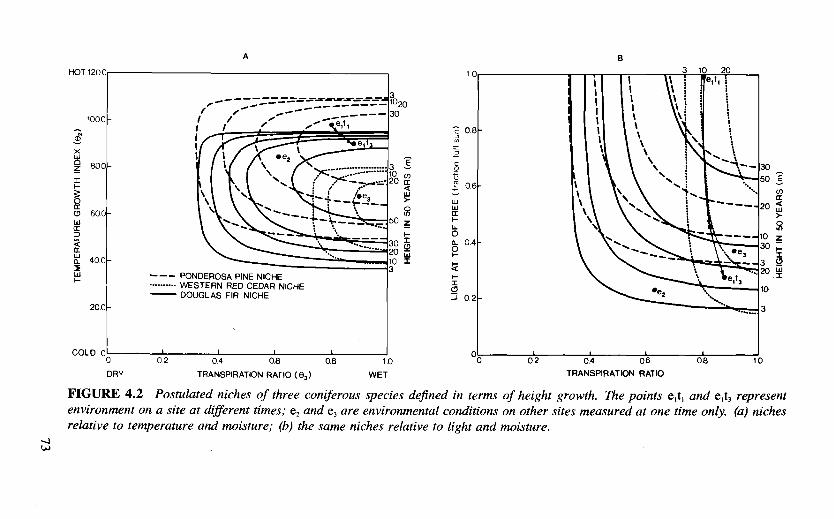
Figure 4.2 shows two 2-dimensional projections of E; the contours de-scribe hypothetical niches for three forest species (ponderosa pine, western redcedar, and Douglas-fir) simulated by our growth model. The environmentalvariables are displayed on the lower and left axes; the species response (simu-lated) is expressed as height after 50 years on the right axis. Three sites arerepresented at points e, e,, and e1. Remember that these points are defined asP(x,y,z) in 3-space, but in our projections P(x,y,z) is illustrated as P(x,y) andP(x,z). The environmental variables used in Figure 4.2 are those discussed inChapter 3 and by Reed and Waring (1974). One of the axes is the temperature-growth index (TGI), which reflects the influence of air and soil temperature ongrowth, and the units of which are optimum temperature days (OTD) (Clearyand Waring 1969; Waring 1969). The axis that reflects moisture supply anddemand is the transpiration ratio of Reed and Waring (1974). This is a ratio ofpotential transpiration on a site to "actual" transpiration computed from on-siteenvironmental data. Potential transpiration is the total amount of water thatwould be lost if there were no stomatal control (an assessment of atmosphericwater demand). The transpiration model includes the effect of stomatal closure,which is a function of plant water stress. When the ratio is equal to 1, that sitehas all the water needed. There is a species-specific lower limit below whichthat species does not occur; so far as we know, all species will grow where theratio is 1 if other factors permit. Waring et al. (1972) present numerous exam-ples of species limits to the transpiration ratio. The third axis is simply lightexpressed as a fraction of full sun.

The trajectory shown fore at time t1 to et3 represents changes in environ-ment on a site over a period of years. In Figure 4. 2a, the site becomes cooler andwetter as the stand develops. Also, note that the trajectory crosses the nicheboundary of Douglas-fir. If other factors (not illustrated) permit, Douglas-fircould become established on the site. Thus a community of ponderosa pine andDouglas-fir would be expected at et3. Also, both species would be expected togrow more than 30 m in 50 years; however, Figure 4.2b shows that the samesite at time t3 would be too dark for good growth. Growth for Douglas-fir at timet3 would be much better than that of ponderosa pine. From Figure 4.2b alone itmight be expected that western red cedar would occur in the community, butfrom Figure 4.2a we see that it would be too hot.

THE NICHE AND SUCCESSION

A community is possible only on sites where the environmental loci arewithin the niche volumes of each species; that is, e(0) e N, where 0 is the set of

A

HOT 1

1 20

100030

i

,/ ,-

400

Ui PONDEROSA PINE NICHE-- WESTERN RED CEDAR NICHE

DOUGLAS FIR NICHE

COLDO' I I I I

0 02 04 06 08 10

B

ic 3_b 20e1t

ii I I

ii I

I I

I t

08

021CI)

LU

z

I

IUI

I

DRY TRANSPIRATION RATIO (83) WET TRANSPIRATION RATIO

FIGURE 4.2 Postulated niches of three coniferous species defined in terms of height growth. The points e,t ande,t3 represent

environment on a site at different times;e2

ande3 are environmental conditions on other sites measured at one time only. (a) niches

relative to temperature and moisture; (b) the same niches relative to light and moisture.


environmental variables and N is the set of niche volumes of the C speciescomposing the community (Reed 1980). Some factors such as fire, althoughimportant for establishment of a species, cannot be conveniently defined alonga continuous ordinate. These factors could be called "trigger variables," andcan be modeled.

As the site's environment changes, its representation, e(0), moves throughE-space; as it crosses a niche boundary, a new community is possible. Thiscould be termed a potential community, or e(0) N, where N is the set of niche

hypervolumes that could be realized on the site. Given an appropriate trigger,the new species can invade, andN becomes equal to N if all possible speciesinvade. The realized community is defined as N. In nature, plant successioncan result from environmental changes on a site over time; prediction of theenvironmental changes could allow prediction of succession. Human activitiesthat result in environmental change can strongly influence forest communitystructure and succession.

The above theory provides a foundation for the work discussed in Hawk etal. (Chapter 2) and Emmingham (Chapter 3). Because a community can existonly where the site locus e is an element of all the nichesN, then the converse isalso true: The location of e in E-space can be defined as the intersection of theset of niches comprising the community (Reed 1980). If the niches of the majorspecies are known, the environmental coordinates of a particular site can bedetermined by simply extrapolating from the point of intersection to the ordi-nates, as did Waring et al. (1972).

A practical application of this theory to land management is possible. If theland were mapped according to vegetation, habitat types, or other plant ordina-tion systems, then the environment or selected community types could bemeasured and the habitat types could be characterized in terms of their environ-mental ranges. Land management practices could be based on knowledge ofmanagement impact on environment, hence community type and productivity.Models cQuld be developed that use environment as input and more directly andaccurately predict ecosystem response to environmental change. Such a modelis discussed below.

THE FOREST GROWTH MODEL (SUCSIM)

The work discussed above defines environment space and can delimitcommunity and niche. The time-trajectories of a site reference locus throughE-space, and the resulting community response, can be simulated by a forestgrowth model. To this end, a forest growth and SUCcession SIMulator (SUC-SIM) based on the above theory was developed (Reed and Clark 1978). Treegrowth is expressed as a function of environment, leaf biomass, and tree size.This growth function can be used to illustrate niche as in Figure 4.2. Naturalestablishment of the forest is simulated according to niche and trigger variables,


and mortality is predicted as a 'function of slow growth and other triggervariables. These ideas, while expressed differently, do not differ greatly frommost forest and tree simulation models (for example, Botkin et al. 1972; Fries1974; Botkin 1977).

A principal disadvantage of most forest growth models is that they requireindividual trees to be grown on small plots. This causes two serious problems:(1) the population must be limited to avoid reaching computer time and sizelimits; and (2) extrapolation from the small plot to more useful units (forexample, quantities perhectare) can be difficult. For example, if the simulationplot size is 0.1 ha, each tree on the plot represents 10 trees/ha; it is impossibleto "kill" fewer than 10 trees/ha. Consequently, to simulate reality, numerousruns with random mortality functions must be made and averaged. This can beprohibitively expensive.

The problem is avoided in SUCSIM, which is so structured that the plotsize can be large. Simulation of a forest requires that the forest be divided intodiscrete plots. The only criterion for determining plot size is the requirementthat environment be relatively homogeneous across the plot. Because the plotsize can be specified at I ha or greater, conversion to useful units is easy andonly one run is required for simulations.

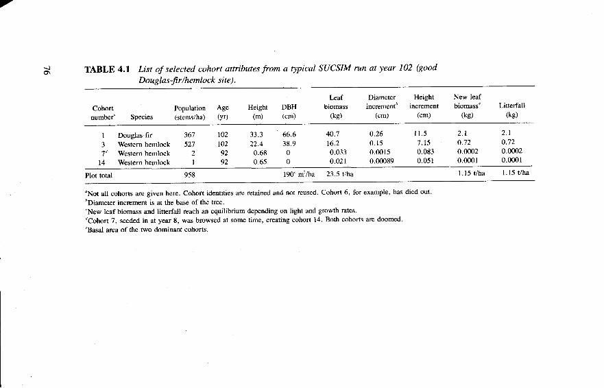
Plots of variable size are simulated easily and efficiently in SUCSIM bygrowing cohorts of trees rather than individuals. A cohort is defined as anobject with a set of attributes including species (with an associated set ofspecific parameters for the growth function, and so on), population, height,diameter, leaf biomass, and age. In SUCSIM these attributes aremore preciselydefined as, for example, "height of trees in cohort i." This can be considered tobe the mean height of the trees in the ith cohort. One species of a given age,height, diameter, and the like is defined as a cohort. This does not imply thatthere is only one cohort per species; there can be n different cohorts of speciesj,each having one or more differences among their attributes. Table 4.1 shows apartial cohort list from a typical SUCSIM run (1-ha plot, 102 years).

The algorithm is simplified and run-time is greatly reduced by use ofcohorts. At each step, the program calls each subroutine (GROW, BROWSE[optionaij, LITTER, DEATH, and so on) once for each cohort. Certain plotattributes, such as light at each level of the stand and fraction of the plot coveredby leaves, are computed after the cohort attributes are updated. The seedingsubroutine (SEED) decides which species to establish, depending on environ-ment. If the environmental coordinates of the stand are within the niche of agiven species, that species can be established. The number of seedlings varieswith environment and the number of other species to be established. OnceSEED has decided which and how many species with an initial height of 3 cmto seed, the system computes the other cohort attributes.

At present there are two ways for trees to die: slow growth and randommortality. As the canopy closes, certain cohorts receive less light and theirgrowth slows. When diameter growth is reduced below a certain species-


A

c

B

SUN

"4'

4'

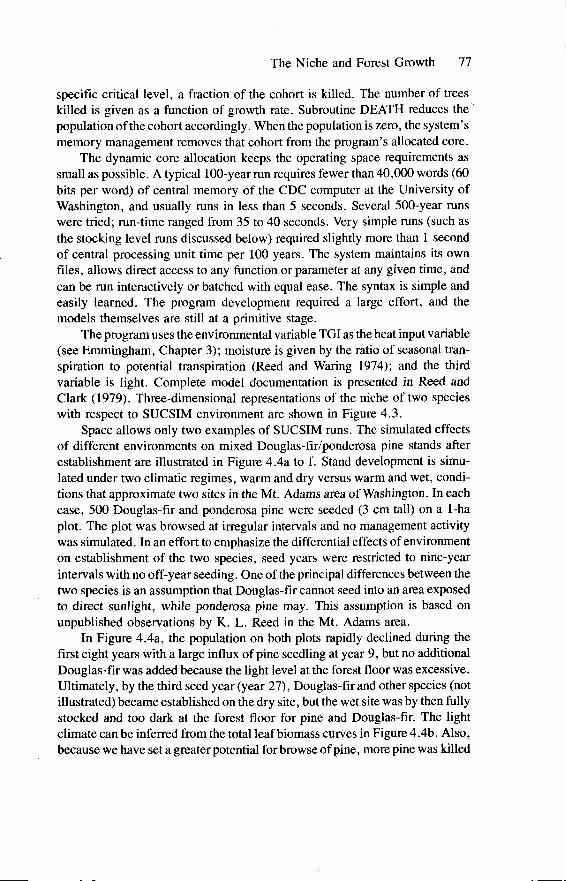
FIGURE 4.3 Three-dimensional representations of the niches of

two species. (a) Douglas-fir niche defined by a minimum heightgrowth of10 m in 50 years; (b) western red cedar niche defined by thesame criteria.


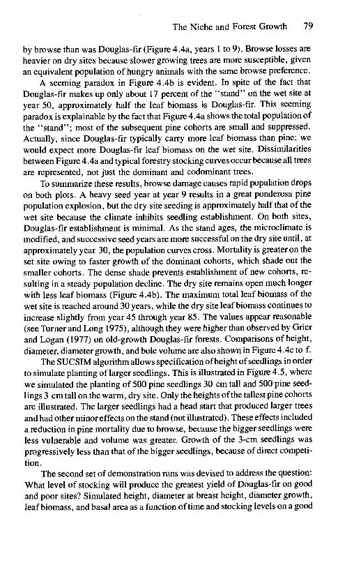
by browse than was Douglas-fir (Figure 4.4a, years ito 9). Browse losses areheavier on dry sites because slower growing trees are more susceptible, givenan equivalent population of hungry animals with the same browse preference.

A seeming paradox in Figure 4.4b is evident. In spite of the fact thatDouglas-fir makes up only about 17 percent of the "stand" on the wet site atyear 50, approximately half the leaf biomass is Douglas-fir. This seemingparadox is explainable by the fact that Figure 4.4a shows the total population ofthe "stand"; most of the subsequent pine cohorts are small and suppressed.Actually, since Douglas-fir typically carry more leaf biomass than pine; wewould expect more Douglas-fir leaf biomass on the wet site. Dissimilaritiesbetween Figure 4 .4a and typical forestry stocking curves occur because all treesare represented, not just the dominant and codominant trees.

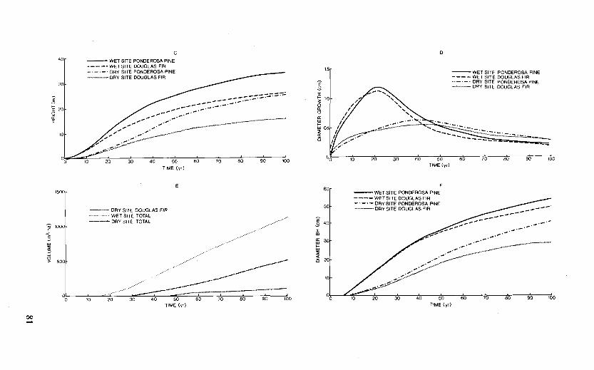
To summarize these results, browse damage causes rapid population dropson both plots. A heavy seed year at year 9 results in a great ponderosa pinepopulation explosion, but the dry site seeding is approximately half that of thewet site because the climate inhibits seedling establishment. On both sites,Douglas-fir establishment is minimal. As the stand ages, the microclimate ismodified, and successive seed years are more successful on the dry site until, atapproximately year 30, the population curves cross. Mortality is greater on theset site owing to faster growth of the dominant cohorts, which shade out thesmaller cohorts. The dense shade prevents establishment of new cohorts, re-sulting in a steady population decline. The dry site remains open much longerwith less leaf biomass (Figure 4.4b). The maximum total leaf biomass of thewet site is reached around 30 years, while the dry site leaf biomass continues toincrease slightly from year 45 through year 85. The values appear reasonable(see Turner and Long 1975), although they were higher than observed by Grierand Logan (1977) on old-growth Douglas-fir forests. Comparisons of height,diameter, diameter growth, and bole volume are also shown in Figure 4 .4c to f.

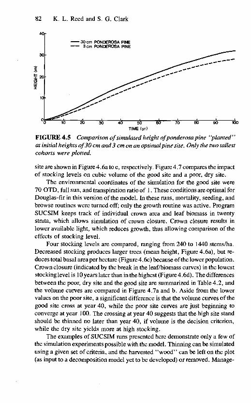
The SUCSIM algorithm allows specification of height of seedlings in orderto simulate planting of larger seedlings. This is illustrated in Figure 4.5, wherewe simulated the planting of 500 pine seedlings 30 cm tall and 500 pine seed-lings 3 cm tall on the warm, dry site. Only the heights of the tallest pine cohortsare illustrated. The larger seedlings had a head start that produced larger treesand had other minor effects on the stand (not illustrated). These effects includeda reduction in pine mortality due to browse, because the bigger seedlings wereless vulnerable and volume was greater. Growth of the 3-cm seedlings wasprogressively less than that of the bigger seedlings, because of direct competi-tion.

The second set of demonstration runs was devised to address the question:What level of stocking will produce the greatest yield of Douglas-fir on goodand poor sites? Simulated height, diameter at breast height, diameter growth,leaf biomass, and basal area as a function of time and stocking levels on a good

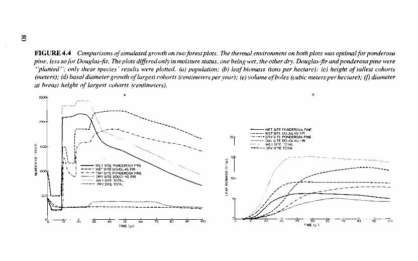
FIGURE 4.4 Comparisons ofsimulated growth on twoforest plots. The thermal environment on both plots was optimalforponderosapine, less so for Douglas-fir. The plots differed only in moisture status, one being wet, the other dry. Douglas-fir and ponderosa pine were"planted"; only these species' results were plotted. (a) population; (b) leaf biomass (tons per hectare); (c) height of tallest cohorts(meters); (d) basal diameter growth oflargest cohorts (centimeters per year); (e) volume ofboles (cubic meters per hectare); (D diameterat breast height of largest cohorts (centimeters).

- WET SITE PONDEROSA PINEWET SITE DOUGLAS FIR

DRY SITE DOUGL AS HR

TIME (yr)90

-WET SITE PONDEROSA PINEWET SITE DOUGLAS FIR

20 - - - DRY SITE PONDEROSA PINEDRY SITE DOUGLAS FIRWET SITE TOTALDRY SITE TOTAL

15

U)(U

- ---

10 ..

0 ..--

TIME (yr)100

C 040 - WET SITE PONDEROSA PINE

WETSITE DOUGLAS FIR ¶5DRY SITE PONDEROSA PINE WET SITE PONDEROSA PINEDRY SITE DOUGLAS FIR ----WET SITE DOUGLAS FIR

- . -. DRY SITE PONDEROSA PINE

0 0 20 30 40 50 60 70 80 90 100 0 10 20 30 60 50 60 70 80 90 10

TIME (yr)TIME (yr)

E60 -WET SITE PONDEROSA PINE

----WET SITE DOUGLAS FIR- - - DRY SITE PONDEROSA PINE

DRY SITE DOUGLAS FIRso DRY SITE DOUGLAS FIR - - - - -.

-WET SITE TOTAL ..

- - --

DRY SITE TOTAL E 40 -- - --. -

,i000 .2E__......

- . --

30 -.---..-.

.--- --------

500 - 20 .---------

._- ---

.-.-- --

-------- 10 - .:-------: - -

00 10 20 30 40 50 60 70 80 90 100

C0 10 20 30 40 50 60 70 80 90 16

TIME (yr) TIME (yr)

00


30cm PONDEROSA PINE-- 3cm PONDEROSA PINE

TIME (yr)

FIGURE 4.5 Comparison of simulated height ofponderosa pine "planted"at initial heights of3O cm and3 cm on an optimal pine site. Only the two tallestcohorts were plotted.

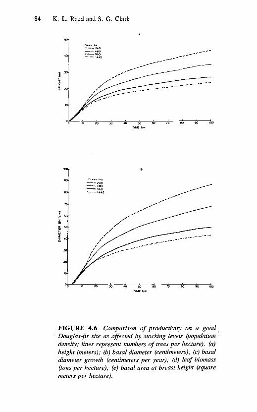
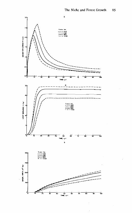
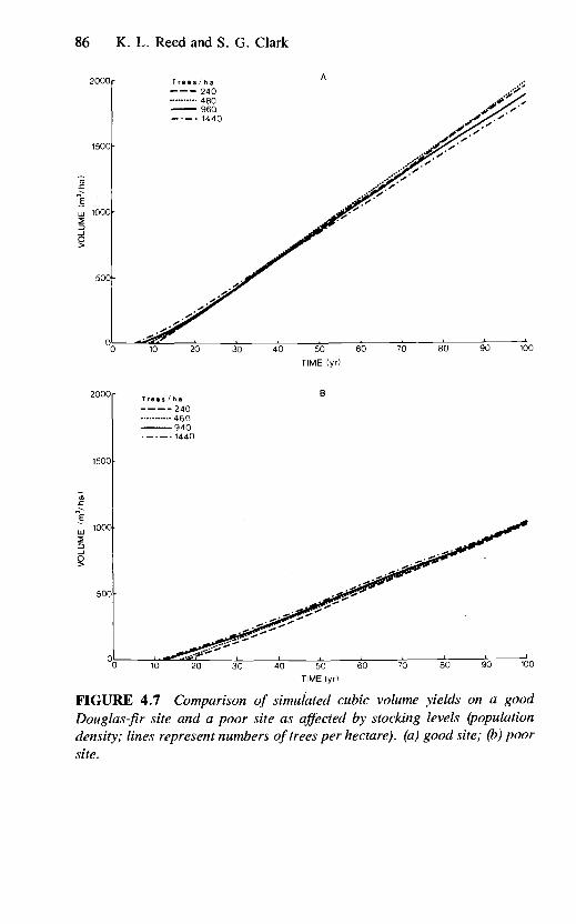
site are shown in Figure 4. 6a to e, respectively. Figure 4.7 compares the impactof stocking levels on cubic volume of the good site and a poor, dry site.

The environmental coordinates of the simulation for the good site were70 OTD, full sun, and transpiration ratio of 1. These conditions are optimal forDouglas-fir in this version of the model. In these runs, mortality, seeding, andbrowse routines were turned off; only the growth routine was active. ProgramSUCSIM keeps track of individual crown area and leaf biomass in twentystrata, which allows simulation of crown closure. Crown closure results inlower available light, which reduces growth, thus allowing comparison of theeffects of stocking level.

Four stocking levels are compared, ranging from 240 to 1440 stems/ha.Decreased stocking produces larger trees (mean height, Figure 4.6a), but re-duces total basal area per hectare (Figure 4. 6e) because of the lower population.Crown closure (indicated by the break in the leaf/biomass curves) in the loweststocking level is 10 years later than in the highest (Figure 4.6d). The differencesbetween the poor, dry site and the good site are summarized in Table 4.2, andthe volume curves are compared in Figure 4.7a and b. Aside from the lowervalues on the poor site, a significant difference is that the volume curves of thegood site cross at year 40, while the poor site curves are just beginning toconverge at year 100. The crossing at year 40 suggests that the high site standshould be thinned no later than year 40, if volume is the decision criterion,while the dry site yields more at high stocking.

The examples of SUCSIM runs presented here demonstrate only a few ofthe simulation experiments possible with the model. Thinning can be simulatedusing a given set of criteria, and the harvested "wood" can be left on the plot(as input to a decomposition model yet to be developed) or removed. Manage-


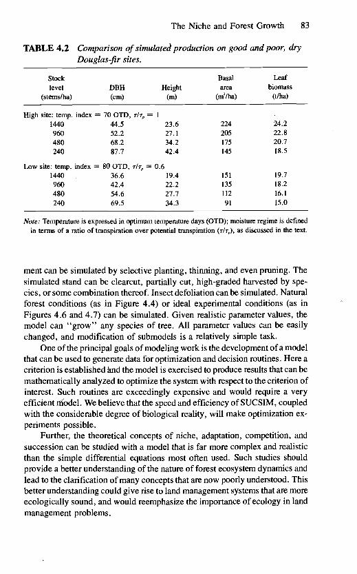
TABLE 4.2 Comparison of simulated production on good and poor, dryDouglas-fir sites.

Stock Basal Leaflevel DBH Height area biomass

(stems/ha) (cm) (m) (m'/ha) (t/ha)

High site: temp. index = 70 OTD, nt,, = 1

1440 44.5 23.6 224 24.2960 52.2 27.1 205 22.8480 68.2 34.2 175 20.7240 87.7 42.4 145 18.5

Low site: temp. index = 80 OTD, nt,, = 0.61440 36.6 19.4 151 19.7

960 42.4 22.2 135 18.2

480 54.6 27.7 112 16.1

240 69.5 34.3 91 15.0

Note: Temperature is expressed in optimum temperature days (OTD); moisture regime is definedin terms of a ratio of transpiration over potential transpiration (n/n,,), as discussed in the text.

ment can be simulated by selective planting, thinning, and even pruning. Thesimulated stand can be clearcut, partially cut, high-graded harvested by spe-cies, or some combination thereof. Insect defoliation can be simulated. Naturalforest conditions (as in Figure 4.4) or ideal experimental conditions (as inFigures 4.6 and 4.7) can be simulated. Given realistic parameter values, themodel can "grow" any species of tree. All parameter values can be easilychanged, and modification of submodels is a relatively simple task.

One of the principal goals of modeling work is the development of a modelthat can be used to generate data for optimization and decision routines. Here acriterion is established and the model is exercised to produce results that can bemathematically analyzed to optimize the system with respect to the criterion ofinterest. Such routines are exceedingly expensive and would require a veryefficient model. We believe that the speed and efficiency of SUCSIM, coupledwith the considerable degree of biological reality, will make optimization ex-periments possible.

Further, the theoretical concepts of niche, adaptation, competition, andsuccession can be studied with a model that is far more complex and realisticthan the simple differential equations most often used. Such studies shouldprovide a better understanding of the nature of forest ecosystem dynamics andlead to the clarification of many concepts that are now poorly understood. Thisbetter understanding could give rise to land management systems that are moreecologically sound, and would reemphasize the importance of ecology in landmanagement problems.


TIME yr1

TIME (yrl

FIGURE 4.6 Comparison of productivity on a goodDouglas-fir site as affected by stocking levels (populationdensity; lines represent numbers of trees per hectare). (a)height (meters); (b) basal diameter (centimeters); (c) basaldiameter growth (centimeters per year); (d) leaf biomass(tons per hectare); (e) basal area at breast height (squaremeters per hectare).


T. y"

25 0

/

IiI/il/I

LIII

I/li

SO 60

TItE tyf)

86 K. L. Reed and S. 0. Clark

E

Ui

-JC>

Ui

TIME (yr)

TIME yrl

FIGURE 4.7 Comparison of simulated cubic volume yields on a goodDouglas-fir site and a poor site as affected by stocking levels (populationdensity; lines represent numbers of trees per hectare). (a) good site; (b) poorsite.


LITERATURE CITED

Bertalanffy, L. von, 1969, General System Theory. Braziller, New York, 289p.Botkin, D. B., 1977, Life and death in a forest: The computer as an aid to

understanding, Ecosystem Modeling in Theory and Practice, C. H. S.Hall and J. W. Day, Jr., eds. Wiley-Interscience, New York, pp. 213-233.

Botkin, D. B., J. F. Janek, and J. R. Wallis, 1972, Some ecological con-sequences of a computer model of forest growth, J. Ecol. 60:849-872.

Cleary, B. D., and R. H. Waring, 1969, Temperature: Collection of data and itsanalysis for the interpretation of plant growth and distribution, Can. J.Bot. 47:167-173.

Emmingham, W H., and R. H. Waring, 1977, An index of photosynthesis forcomparing forest sites in western Oregon, Can. J. For. Res. 7:165-174.

Franklin, J. F., and C. T. Dyrness, 1973, Natural vegetation of Oregon andWashington, U.S. Department of Agriculture Forest Service GeneralTechnical Report PNW-8, Portland, Oreg., 4l'lp.

Fries, J., 1974, Growth models for tree and stand simulation. Royal CollegeForest Bulletin No. 30, Stockholm, 379p.

Green, R. H., 1971, A multivariate statistical approach to the Hutchinsonianniche: Bivalve molluscs of central Canada, Ecology 52:543-556.

Gner, C. C., and R. S. Logan, 1977, Old-growth Pseudotsuga menziesiicommunities of a western Oregon watershed: Biomass distribution andproduction budgets, Ecol. Monogr. 47:373-400.

Grinnell, J., 1917, The niche-relationships of the California thrasher, Auk34:427-433.

Hutchinson, G. E., 1957, Concluding remarks, Cold Spring Harbor Symp.Quant. Biol. 22:415-427.

Klir, G. J., 1969, An Approach to General Systems Theory, Van NostrandReinhold, New York, 323p.

Maguire, B., 1973, Niche response structure and the analytical potentials of itsrelation to the habitat, Am. Nat. 107:213-246.

Mason, H. L., and H. H. Langenheim, 1957, Language analysis and theconcept Environment, Ecology 38:392-404.

Reed, K. L., 1980, An ecological approach to modeling growth of forest trees,For. Sci. 26:33-50.

Reed, K. L., and S. G. Clark, 1979, SUCession SIMulator: A coniferous forestsimulator, Model documentation, US/IBP Coniferous Forest BiomeBulletin No. 11, University of Washington, Seattle, 96p.

Reed, K. L., and R. H. Waring, 1974, Coupling of environment to plantresponse: A simulation model of transpiration, Ecology 55:62-72.

Turner, J., and J. N. Long, 1975, Accumulation of organic matter in a series ofDouglas fir stands, Can. J. For. Res. 5:681-690.

Waring, R. H., 1969, Forest plants of the eastern Siskiyous: Theirenvironmental and vegetational distribution, Northwest Sci. 43:1-17.


Waring, R. H., K. L. Reed, and W. H. Emmingham, 1972. An environmentalgrid for classifying forest ecosystems, in ProceedingsResearch onConiferous Forest EcosystemsA Symposium, J. F. Franklin, L. V.Dempster, and R. H. Waring, eds., U.S. Department of AgricultureForest Service, Portland, Oreg., pp. 79-91.

Whittaker, R. H., and S. A. Levin, eds., 1975, Niche: Theory and Application,Dowden, Hutchinson & Ross, Stroudsburg, Pa., 464p.

Whittaker, R. H., S. A. Levin, and R. B. Root, 1973, Niche, habitat andecotype, Am. Nat. 107:321-328.

Zobel, D. B., A. McKee, G. M. Hawk, and C. T. Dyrness, 1976,Relationships of environment to composition, structure, and diversity offorest communities of the central western Cascades of Oregon, Ecol.Monogr. 46:135-156.

The Niche and Forest Growth - Oregon State University

Documents

Transcript of The Niche and Forest Growth - Oregon State University