The mosaic of high performance Domain …€¦The mosaic of high performance Domain Decomposition...

The mosaic of high performance Domain Decomposition Methods for Structural Mechanics: Formulation, interrelation and

numerical efficiency of primal and dual methods

Yannis Fragakis, Manolis Papadrakakis

Institute of Structural Analysis & Seismic Research National Technical University Athens

9, Iroon Polytechniou, Zografou Campus GR-15780 Athens, Greece

(fragayan , mpapadra)@central.ntua.gr

Technical Report First version: June 10, 2002

1st revision: January 29, 2003 2nd revision: May 19, 2003

To appear in Computer Methods in Applied Mechanics and Engineering, 2003

Abstract

A multitude of Domain Decomposition Methods (DDM) for Structural Mechanics is available in the literature today. A unified framework for formulating primal and dual DDM is thus presented in this paper, aiming at providing a mathematical platform for a uniform treatment of high per-formance DDM in Structural Mechanics. A novel approach for develop-ing new DDM from existing methods is also proposed and is applied to dual and primal methods. In the field of the FETI methods, this approach leads to a new category of methods derived from existing FETI variants. Furthermore, two alternative formulations of the Balancing Domain De-composition method are described, while interrelations between the in-troduced and existing methods are established. Finally, comparative nu-merical tests demonstrate the differences in the computational perform-ance of the methods in question.

Y. Fragakis, M. Papadrakakis, Technical Report, NTUA, Athens, 2003

1 Introduction

In the last two decades, extensive research efforts have been devoted to the development of efficient solution methods for finite element simulations and have led to the develop-ment of several high performance solvers. Domain Decomposition Methods (DDM) consti-tute today an important category of methods for the solution of a variety of problems in Computational Mechanics. Their performance in both serial and parallel computer envi-ronments is demonstrated in a number of papers and conferences specialized in DDM over the last decade. In fact, DDM have gradually become the main field of interest of a large number of researchers and have started making their way into high performance commer-cial software applications.

In Structural Mechanics, the most popular DDM can be divided in two major categories, the Primal and Dual Substructuring Methods. In the early 90s, an important dual DDM, the Finite Element Tearing and Interconnecting (FETI) method was introduced by Farhat and Roux [FR91]. Since their introduction, FETI and several variant methods have gained a high importance and today are considered as highly efficient DDM. Furthermore, an im-portant family of primal DDM are considered to be the Balancing Domain Decomposition (BDD) methods, introduced by Mandel [Man93]. Research in BDD and FETI methods has been progressing in parallel since their introduction and both methods are currently capa-ble of successfully addressing a large number of complex problems in Computational Me-chanics.

Today, a number of DDM versions exist in the literature capable of handling homoge-neous or heterogeneous problems, that is problems with similar or different stiffness coef-ficients across the subdomain interfaces. Furthermore, dual DDM are often implemented with different definitions of the Lagrange multipliers which represent the interaction forces between the subdomains, thus leading to different formulations. Due to this variety of DDM versions proposed in the past, a large number of theoretical findings and implemen-tation techniques that are available in the literature for both primal and dual methods, are not correlated to each other through a consistent formulation. For this reason, a unified framework for formulating both primal and dual DDM is presented in this paper, aiming at providing a mathematical tool for uniform treatment of the high performance DDM in Structural Mechanics. The formulation of standard DDM (like the Primal Substructuring Method (PSM) and the FETI methods) is then revisited in the context of the proposed uni-fied framework.

Furthermore, primal preconditioners are proposed in this paper by implementing an idea that allows the construction of preconditioners for PSM, based on the theory of DDM that incorporate a coarse problem, like for example the FETI methods. A primal category of methods is thus created from the FETI methods. The relations between the new methods and the FETI methods are then investigated.

Following the development of PSM preconditioners based on existing FETI methods, two alternative formulations of the BDD are described. The relations between the intro-duced methods and existing DDM are then used to prove a connection between the BDD method and an instance of the FETI method. In addition, the newly introduced and previ-ously known methods are compared in numerical tests. Many issues treated in this paper have also been included in [FP02a,FP02b].

The remainder of this paper is organized as follows. Section 2 presents a theoretical framework for mapping the displacements and forces of the subdomains on the global do-main. Relations between mapping matrices that are extensively used in subsequent sections

2


are also outlined. The treatment of local subdomain and interface problems is then de-scribed in section 3. Subsequently, sections 4 and 5 outline the basic theory of the PSM and FETI methods. The primal methods derived from FETI variants are then introduced in section 6, followed by an analysis of their relations to existing FETI methods. Further-more, section 7 refers to the BDD method, while the relation between the BDD and FETI methods is treated in section 8. Section 9 presents numerical tests performed in order to compare the discussed methods and concluding remarks are provided in section 10.

2 Mapping subdomains on the global domain

This section presents a theoretical framework for mapping the displacements and forces of the subdomains on the global domain. The introduced framework treats uniformly the scaling of DDM for homogeneous or heterogeneous problems and for different Lagrange multiplier definitions. It has to be clarified that this section does not treat the mapping of subdomains from the point of view of computer implementation, but it presents the theory of a unified theoretical framework for subdomain mapping from the point of view of mathematical formulation of the DDM. In particular, different choices that have been used in the past in the formulation of DDM in Structural Mechanics are integrated in general-ized equations. We then state previously known as well as new relations, which connect the mapping matrices that are used in this section. The presented relations are used exten-sively in subsequent sections of this paper.

2.1 Mapping displacements and applied loads of the subdomains

If and u f are the displacement and applied loads vectors of the global domain and ( )su and ( )sf are the corresponding vectors of the subdomains 1,..., ss N= , then these global and local subdomain variables are connected with the relations

(1) TTT ( )(1) sNsu u u L= u =

TTT ( )T T (1) sNsf L f L f f = = (2)

where is a Boolean mapping matrix that is usually referred to as a global to local map. Restricting equations (1) and (2) to the d.o.f. that belong to the interface between subdo-mains, we obtain the equations

L

(3) TTT ( )(1) sNs

b b b bu u u L = bu=

TT T

( )T T (1) sNsb b b b b bf L f L f f = = (4)

where subscript denotes the restriction of a matrix or vector to d.o.f. that belong to the boundaries between subdomains.

b

In DDM it is often needed to split an interface force vector bf between the subdomains, or to estimate an interface displacement vector u from different subdomain values b

sbu . In

these operations it is favorable to take into account the possible heterogeneity between the

3


subdomains. Such operations are often performed within the preconditioning step of DDM and may be expressed by the formulas

Testimate b

sbu L= p bu

b

(5)

estimate b

sb pf L f= (6)

In eqs. (5) and (6), if the underlying problem is homogeneous, is set equal to bpL

1bp b bL L M −= (7)

where bM denotes a diagonal scaling matrix with each diagonal entry being equal to the multiplicity of the corresponding d.o.f, which is equivalent to the number of its neighbor-ing subdomains. For heterogeneous problems, however, it is more appropriate to scale ma-trix with respect to the subdomain stiffness coefficients. In this case, matrix takes the form

bpLbpL

T(b

s sp b b b b bL D L L D L 1)−= (8)

with sbD denoting a diagonal matrix where each diagonal entry is equal to the diagonal

element of the subdomain stiffness matrix of the corresponding d.o.f. It should be noted that any matrix L of eqs. (7) and (8) may in fact be used for both homogeneous and het-erogeneous problems. The distinction between homogeneous and heterogeneous is made here, because

bpL of eq. (7) is best suited for homogeneous problems, while bpL of eq. (8)

is best suited for heterogeneous problems. Therefore, in the rest of this paper whenever homogeneous or heterogeneous cases are examined, the most suitable scaling operator is implicitly assumed.

bp

Similarly to eqs. (1) to (4), eqs. (5) to (8) may be expanded to include internal d.o.f. of the subdomains

T sestimate pu L= u (9)

sestimate pf L f= (10)

where for homogeneous cases is given by pL

1pL LM −= (11)

and for heterogeneous cases

T(s spL D L L D L 1)−= (12)

In eqs. (11) and (12), matrices M and sD are formed similar to matrices bM and sbD , but

they are now expanded to include both the interface and the internal d.o.f. of the subdo-mains.

2.2 Mapping Lagrange multipliers on the subdomains

In a number of DDM, as for example in FETI methods, it is required to define the nodal interaction forces between the subdomains. These interface tractions are also used to en-

4


force the interface displacement compatibility between subdomains and are commonly re-ferred to as Lagrange multipliers in DDM literature. Among infinite possible ways to de-fine the Lagrange multipliers, we note the non-redundant, redundant and orthonormal choices which have been used in the FETI methods [FR94,PJF97,JPF97]. These three dif-ferent choices are depicted in Fig. 1 for a node belonging to three subdomains. For each d.o.f. of the node of Fig. 1, the subdomain forces

b

sfλ which are due to the Lagrange multi-pliers λ , are given by:

For non-redundant multipliers:

(1)

1(2) T

2(3)

1 01 1

0 1

b

b b

b

sb

ff f

f

λ

λ λ

λ

λB λ

λ

= = − = −

(13)

For redundant multipliers: 1

T2

3

1 0 11 1 0

0 1 1b

sbf Bλ

λλ λλ

− = − =

−

(14)

For orthonormal multipliers: 1 T

2

1 2 1 6

1 2 1 6

0 2 6b

sbf Bλ

λλ

λ

−

= − − =

(15)

Note that in the orthonormal case, bB satisfies Tb bB B I= . It should be further noted that

the subdomain interaction forces can also be mapped using a three-field formulation, which has been proven equivalent to the orthonormal choice of Lagrange multipliers [PJF97,JPF97] and to the redundant choice [RFTM99].

Given a Lagrange multiplier vector λ , the applied forces on the interface nodes of the disconnected subdomains may be expressed as Ts

b bf B λ− . If we also include the internal d.o.f. of the subdomains, the applied forces take the form Tsf B λ− , where matrix bB has been expanded to B . The B and bB mapping matrices may also be used to express the displacement compatibility condition at subdomain interfaces as

3

1 1 22 21

3 3

a) Non-redundant b) Redundant c) Orthonormal

Figure 1. Different definitions of Lagrange multipliers for a

node belonging to three subdomains

5


(16)

(1)

( )(1)

( )

0s

s

bNs

b b b bN

b

uB u B B

u

= =

or

(17)

(1)

( )(1)

( )

0s

s

Ns

N

uBu B B

u

=

=

In the past, a number of modified versions of bB that incorporate scaling effects for homogeneous or heterogeneous problems, have been used in preconditioning steps of DDM. Thus, for homogeneous problems, the following

bpB matrices can be written, as modified variations of bB :

a) For non-redundant Lagrange multipliers: ( ) 1Tbp b b bB B B B

−= (18)

b) For redundant Lagrange multipliers: 1

b

sp b bB B M

−

= (19)

c) For orthonormal Lagrange multipliers: bp bB B= (20)

For heterogeneous problems the corresponding matrices are the following:

a) For non-redundant or orthonormal Lagrange multipliers: ( )1 11T

b

s sp b b b b bB B D B B D

− −−= (21)

b) For redundant Lagrange multipliers: 1ˆ

b

sp b bB D B Dλ

−

= (22)

In eq. (19), sbM is a diagonal matrix that stores in each diagonal entry the multiplicity of

the corresponding d.o.f. Matrix Dλ of eq. (22) is also diagonal with each diagonal element being equal to the product of the two respective diagonal elements of the subdomain stiff-ness matrices of the d.o.f. that are attached to the corresponding Lagrange multiplier, di-vided by the diagonal element of the corresponding d.o.f. of matrix . For example,

the diagonal entry of

T sb b bL D L

Dλ related to the first Lagrange multiplier defined in eq. (14) is equal to ( )11 22 22k k + +11k k 33k , where denotes the diagonal element of the subdomain stiff-ness matrix of the corresponding d.o.f. Matrices

iik

bpB of eqs. (19) and (22) are used in the FETI methods with redundant Lagrange multipliers [RFTM99,RF99,BDFL+00], while ma-trix

bpB of eq. (21) was first used in a FETI method for non-redundant Lagrange multipli-ers in [KW01]. Finally, we note that the subscript is used in P

bpB and in other matrices of this section, in order to denote that these matrices are usually used in preconditioning steps.

Furthermore, eqs. (18) - (22) can be expanded to include both internal and interface d.o.f. of the subdomains.. The corresponding expressions for matrix pB are obtained by simply removing subscript from all matrices in these equations. b

6


2.3 Connections between subdomain mapping matrices

In this subsection, we present a number of relations connecting the subdomain mapping matrices introduced in the previous sections. The displacement and Lagrange multiplier mapping matrices of the previous sections satisfy the relations

and range( ) null( )bL = bBbpBrange( ) null( )

bpL = (23)

0b bB L = and 0b bp pB L = (24)

Tbb pL L I= (25)

and T 2 T( )bp b p bL L L L=

b b

T 2 T( )bb p b pB B B B= (26)

T Tb bp b b pL L B B I+ = (27)

Eqs. (23) to (27) hold for any of the discussed definitions of Lagrange multipliers and for homogeneous or heterogeneous problems. To be more pricise, eqs. (23) to (27) hold in the following cases: a) Case of homogeneous scaling: is set equal to eq. (7) and

bpLbpB is selected equal to any

of eqs. (18) – (20), and (b) Case of heterogeneous scaling: is set equal to eq. (8) any

bpLbpB is selected equal to

any of eqs. (21) – (22). The proofs of the above equations are omitted for the sake of brevity. These proofs are in fact similar to those provided in [RFTM99] for redundant Lagrange multipliers and homo-geneous problems. Proofs for eq. (27) can also be found in [KW01].

In contrast to eqs. (23) to (27), the subsequent equations of this section hold for specific choices of Lagrange multipliers and homogeneous or heterogeneous scaling. For instance, relation

Tbb pB B I= (28)

holds for non-redundant or orthonormal Lagrange multipliers, while it does not hold in general for redundant multipliers.

Furthermore, in the case of homogeneous problems, it follows from eqs. (7) and (27) that

T T

1 Tb bb p p b

b b b

B B I L L

I L M L−

= −

= − (29)

In eq. (29), matrix 1 Tb b bI L M L−− is symmetric. Hence, in homogeneous problems both ma-

trix Tbb pB B and matrix T

bp b1 T

b b bL L L= M L− are symmetric, while in general this is not the case for heterogeneous problems. For homogeneous scaling, we thus have

Tbp b b pb

L L L LΤ= and Tb bb p p bB B B BΤ= (30)

In further sections of this paper, we generally make use of eqs. (23) to (27), which hold for all three definitions of Lagrange multipliers and homogeneous or heterogeneous prob-lems. When however eqs. (28) or (30) are used, we specify the particular version – homo-

7


geneous or heterogeneous scaling and Lagrange multiplier definition – for which the re-lated mathematical expressions and numerical algorithms hold. It can easily be deduced that all equations of this subsection also hold after removal of subscript b .

3 Solving the local subdomain and interface problems

3.1 Solving the local subdomain problems

Several DDM, like the FETI methods, require the solution of local subdomain prob-lems of the form

T( ) ( ) ( ) ( )s s s sK u f B λ= − , 1,..., ss N= (31)

where ( )sK is the stiffness matrix of subdomain . Eqs. (31) may be gathered to form one matrix equation using block diagonal notation

s

T

T

(1) (1) (1) (1)

T

( ) ( ) ( ) ( )s s ss

s s s

N N N N

K u fK u f B

K u f B

Bλ λ

= − ⇔ = −

(32)

The solution of eq. (31) takes two different forms, depending on the presence or not of zero energy modes in the subdomains. In the case of a non-floating subdomain, that is a subdomain whose external constraints prevent all possible zero energy motion, the solution of eq. (31) is

1( ) ( ) ( ) ( )(s s s su K f B

T

)λ−

= − (33)

On the other hand, in the more general case of a floating subdomain, eq. (31) is solvable if the loads

T( ) ( )s sf B λ− are self-equilibrated, that is if

T T( ) ( ) ( )(s s sR f B λ) 0− = (34)

where matrix ( )sR stores in its columns the zero energy modes of subdomain . If condi-tion (34) holds, then the general solution of eq. (31) is given by

s

T( ) ( ) ( ) ( ) ( ) ( )( )s s s s su K f B R aλ

+

= − + s (35)

where +( )sK is a generalized inverse of ( )sK and ( )sα is a vector of arbitrary entries that

represent the amplitudes of the zero energy modes. Similarly to eq. (31), eqs. (33) - (35) may be written in block diagonal notation, as

T T(s sR f B λ 0− ) = (36)

T

( )s s s su K f B Rλ+

= − + a (37)

where ,

+

+

(1)

( )s

s

N

KK

K

+

=

(1)

( )s

s

N

RR

R

=

and (38)

(1)

( )sN

aa

a

=

8


For non-floating subdomains, submatrices ( )sK+

of sK+

are substituted by 1( )sK

−

and sR and a are modified accordingly, to satisfy eqs. (33) and (35).

In DDM, the equations which are related to internal d.o.f. of the subdomains are often eliminated first. For that purpose, eq. (32) is transformed to

Tˆs s sb b bS u f B λ= − (39)

where

,

(1)

( )s

s

N

SS

S

=

1( ) ( ) ( ) ( ) ( )s s s sbb bi ii ibS K K K K

−

= − s , 1,..., ss = N (40)

and

1ˆ s s s s

b b bi iis

if f K K f−

= − (41)

Subscripts and i denote the restriction of the matrices to interface and internal d.o.f., respectively.

b( )sS is a condensed stiffness matrix, also called Schur complement.

Following the reasoning of eqs. (36) and (37), a solution of eq. (39) exists under the condition

T Tˆ(s s

b b bR f B λ 0− ) = (42)

and is given by

Tˆ(s s s sb b bu S f B Rλ

+

= − ) + ba (43)

where sbR denotes the restriction of sR to the interface d.o.f.

The generalized inverse matrices used in this section are related to the stiffness matrices of the subdomains with the following property: For a generalized inverse sK

+

(or sS+

) of sK (or sS ) there is a matrix Y such that

s sK K I R Y+

= + s (or s sbS S I R Y

+

= + s

=

) (44)

Furthermore, we have

and range( ) null( ) 0s s s sR K K R= ⇒ range( ) null( ) 0s s s sb bR S S R= ⇒ = (45)

Eqs. (44) and (45) imply that

s s sK K K K+ s= and s s sS S S S

+ s= (46)

3.2 Solving the interface problem

In Structural Mechanics, a number of DDM employ the Preconditioned Conjugate Gra-dient (PCG) method to solve iteratively the interface problem. In this section, we outline the standard PCG algorithm, which is used in this paper as a basis for the different proofs provided in subsequent sections. Thus, given a linear system of equations Ax b= , where

is symmetric positive semi-definite and a preconditioning matrix , the PCG algo-rithm proceeds as follows: A 1A−

9


4 The Primal Substructuring Method

A basic DDM is the Primal Substructuring Method, abbreviated in the following as PSM. In the context of this DDM, the internal d.o.f. of the subdomains are eliminated first. The PSM interface displacement problem is thus obtained by combining eqs. (3), (4) and (39) in order to form the equation

ˆˆbSu fb= (47)

where

and Tˆ sbS L S L= b

ˆTˆ sb b bf L f= (48)

The solution of the linear system of eqs. (47) is usually performed with the PCG method. In the past, several strategies have been proven efficient for preconditioning the PCG

for these types of problems (see for example [Man93, LV97, BPK97]). A quite common choice is the preconditioner

1 Tb

sp bpA L S L

+− = (49)

which is used in the so-called Neumann-Neumann PSM. More precisely, the precondi-tioner (49) is implemented as follows:

(50) 1 T T

b

s s sp b b pA L N K N L

+− =b

0

• Initialize 0 0r b Ax= − , , 0 1z A r−= 0 0p z=

0q Ap= 0 , T

T

0 00

0 0

p rp q

η =

• Iterate until convergence 1,2,...k =

Estimate of the solution 1 1k k k k 1x x pη− − −= + Residual 1 1k k k kr r qη 1− − −= − Preconditioned residual 1k kz A r−=

a) No reorthogonali-zation case

T

T1

1 1

k kk k k

k k

z rp z pz r

−− −

= + Search vector b) Reorthogonaliza-

tion case

T

T

1

0

k ikk k

i ii

z q ip z pp q

−

=

= −∑

Product of search vector by A k kq Ap=

a) No reorthogonali-zation case

T

T

k kk

k k

z rp q

η = Step length b) Reorthogonaliza-

tion case

T

T

k kk

k k

p rp q

η =

10


where sbN is a Boolean matrix which extracts the interface d.o.f. from subdomain d.o.f.

vectors, as in eqs.

s s sb bu N u= and s s s

b bf N f= . (51)

Further on in this paper, sS+

is often used in place of Ts s s

bN K N+

b for brevity. Matrix Ts s s

bN K N+

b is thus the particular generalized inverse of sS that is implicitly assumed, in the rest of the paper. Another important class of efficient preconditioners for the PCG method implemented within the PSM are those used in the Balancing Domain Decomposition methods, which were introduced in [Man93] and are discussed in further sections.

5 The FETI Method

The Finite Element Tearing and Interconnecting (FETI) method, is a dual DDM that has been implemented for a number of problems in Computational Mechanics. Since its intro-duction [FR91], it has attracted a lot of attention and is today considered as a fast domain decomposition algorithm suitable for both serial and parallel computing environments.

While its predecessor, the PSM, performs iterations in order to compute the interface displacement vector u of the structure, the FETI method iterates on the Lagrange multi-plier vector

b

λ . The Lagrange multipliers, that is the interaction forces between the subdo-mains are dual with respect to the interface displacements and this explains the name Dual Substructuring Method, in comparison to Primal Substructuring Method.

In the context of the FETI method, the nodal force vector f of the structure is first split to the subdomains:

spf L f= (52)

Combining eqs. (17), (36) and (37), the following system is obtained

T 0IF G d

G aλ−

= e− −

(53)

where TsIF BK B

+

= , sG B , R= s sd BK f+

= and Ts se R f= (54)

In order to decouple the linear system (53), the projection operator

(55) T 1( )P I QG G QG G−= − T

is used. Eq. (55) defines the operator for a square matrix Q . satisfies the eqs. P P

T 0G P = (56)

0PQG = (57)

2P P= (58)

Premultiplying the first of the two matrix equations in (53) with , it fol-lows that for a given Lagrange multiplier vector

T 1 T( )G QG G Q−

λ , the vector of the zero energy mode amplitudes is equal to a

11


( ) (1T TIa G QG G Q d F )λ−

= − − (59)

Furthermore, using eqs. (37) and (59), it follows that the jump sbu Bu∆ = of the displace-

ment field at subdomain interfaces is equal to

T (sb Iu Bu d F Ga P d FIλ λ∆ = = − + = − ) (60)

Note that eq. (60) implies that the interface displacement jump bu∆ satisfies the condition

T 0bG Q u∆ = (61)

Based on eq. (60), the linear system (53) may easily be proven equivalent to the following system of equations, in which vectors λ and are decoupled: a

( ) ( )1

T T

(62.a) (62.b)

(62.c)

T TI

IITT

a G QG G Q d FF Ga d

P F P dG e

G e

λλ

λλ

λ

− = − − − = ⇔ = = =

In order to solve eqs. (62.b) and (62.c) for the Lagrange multiplier vector λ , the following splitting of the Lagrange multipliers is performed

Pλ λ0= + λ (63)

where λ0 is a vector satisfying (62.c). The component λ0 is chosen as

(64) T( )QG G QG eλ −0 =

1

which satisfies (62.c). Based on eqs. (63) and (64), the system of the eqs. (62.b) and (62.c) can thus be written as

T T( ) (IP F P P d F )Iλ λ0= − (65)

The one-level FETI (FETI-1) method consists in applying the PCG algorithm to eq. (65) in order to compute the Lagrange multiplier vector λ . This method was named one-level, in order to be distinguished from the so-called two-level FETI (FETI-2) method, which was later proposed for faster solution of plate and shell problems [FM98,FCMR98]. An-other more recently proposed variant of the FETI method which should be noted is the dual-primal FETI (FETI-DP) method [FLLP+01,FLP00].

The FETI-1 algorithm is completed as follows: After computing the Lagrange multiplier vector λ by applying the PCG algorithm to eq. (65), the amplitudes of the subdomain rigid body modes are computed from eq. (62.a). Subdomain displacement fields

asu are

then computed from eq. (37) and the total displacement field of the structure is finally given by

u

T spu L u= (66)

It should further be noted that if kλ , and kz kp are the k-th solution estimate, precon-ditioned residual and search vector, respectively, of the PCG applied for the solution of eq. (65), then the PCG algorithm can be written in an alternative form in order to operate di-rectly on the vectors

k kPλ λ λ0= + , kz Pzk= and k kp Pp= (67)

12


The corresponding algorithm, which is given in [FR94,FPL00] and other publications, is usually used instead of the standard PCG algorithm in order to solve eq. (65).

5.1 Preconditioners for the FETI method

Two preconditioners are more often used in the FETI method:

a) (Dirichlet preconditioner) (68) 1 T

b

D sI pF B S B

−

=bp

bpb) (Lumped preconditioner) (69) 1 T

b

L sI p bbF B K B

−

=

The Dirichlet preconditioner is typically used in fourth-order problems. Moreover, in sec-ond-order problems the Lumped preconditioner is usually more efficient in terms of the total solution time. In some second-order problems however, namely in highly heterogene-ous structures and in problems where subdomains of bad aspect ratio are generated, the Dirichlet preconditioner may outperform the lumped one [BDFL+00]. Variant forms of the Dirichlet preconditioner using approximate expressions for s

iiK of the Schur complement 1s s s s

bb bi ii ibS K K K K−

= − s , have also been tested in [CP02].

5.2 Projection operators for the FETI method

For homogeneous problems, operator defined in eq. (55) is usually implemented with . However, for heterogeneous problems matrix Q is set equal to one of the following

three choices:

PQ I=

a) 1D D

IQ F−

= (Dirichlet preconditioner) (70)

b) 1L L

IQ F−

= (Lumped preconditioner) (71)

c) (superlumped matrix) (72) Tb d

SL sp bb pQ B K B=

b

where d

sbbK denotes a diagonal matrix whose main diagonal is equal to the main diagonal

of sbbK . The superlumped choice of eq. (72) has been recently proposed in a discussion of

highly heterogeneous problems in [BDFL+00]. In the FETI operator of eq. (55), it is required to solve linear problems of the form P

( )TG QG x b= (73)

The linear system (73) constitutes the so-called “coarse-grid” problem of the FETI method. This name is explained by the fact that is a sparse matrix, with the typical sparsity pattern of a finite element stiffness matrix, if one considers each subdomain as a finite ele-ment node having the same number of d.o.f. as the number of its zero-energy modes. The coarse problem of FETI ensures the exchange of information between remote subdomains of the structure at each FETI iteration. It thus guarantees fast convergence of the PCG al-gorithm.

TG QG

13


6 A family of FETI derived preconditioners for the Primal Substructuring Method

In this section, we introduce a new category of preconditioners for the PSM. The PCG is applied for the solution of eq. (47) in order to compute the interface displacement vector

, given an interface force vector bu bf . A good preconditioner for the PSM must treat the

k-th PCG residual as applied forces on the interface nodes of the structure and return in a good estimate of the interface displacements of the structure for the applied forces . For instance, if the PSM preconditioning step is performed with any solver, like for example the FETI method, the PCG will immediately converge in the first iteration. We therefore propose to use as preconditioner of the PSM, a crude approximation of the FETI solution and as such we choose the first estimate for the interface displace-ments of the structure obtained from the first iteration of the FETI method.

ˆ ˆkbr f Su= −

1k kz A r−

kr

kb

=

For example, consider the FETI-1 algorithm with an applied forces vector f equal to

T kbf N r= (74)

where is the k-th residual of the PSM and is a Boolean matrix which extracts the interface d.o.f. from a vector with the size of all d.o.f. of the structure, as in eqs. and

kr

b

bN

b bu N u=

bf N f= . Since all forces in the load vector of eq. (74) are applied on the interface nodes of the structure, we have k

bf r= and 0f si = . Furthermore, the interface forces bf

may be split to the subdomains with the equation

b b

s kb p b pf L f L r= = (75)

From eqs. (41) and (75), it follows that ˆb

s sb b p

kf f L r= = . The components e and d of eqs.

(54) thus become T Ts s s

bf R r= = ke R and b

s s sb pB S L r

+ k

b

d BK f+

= = . We also note that with

respect to interface values, matrix of eqs.(54) may be written as . Furthermore, the initial Lagrange multiplier vector

IF T Ts sF B B B S B+ +

= =I bKλ0 of eq. (64) is equal to

TT 1( ) s k

bQG G QG R rλ −0 = (76)

From eq. (62.a) it follows that the zero energy mode amplitudes a0 , which correspond to the initial Lagrange multiplier vector λ0 , may be expressed by the relation

( ) ( )

( ) ( )

1

0

1 T0b

T TI

T T s kb p b

a G QG G Q d F

G QG G QB S L r B

λ0

λ+

−

−

= − −

= − − (77)

The above analysis combined with eqs. (5) and (43) leads to the following interface dis-placements estimated from the initialization of the FETI-1 algorithm:

0bu

14


( )( )( ) ( )( ) ( )

0

T

T

T T0 0

T T 1 T0 0

T 1 T0

T 1 T T 1

ˆ(

( ( ) (

( )

( ) ( )

b

b

b b

b b

b b

sb p b

s s sp b b b

s k s T T s kp b b b p b

s T T s kp b b p b

)

s T T s sp b b b b p

u L u

L S f B R a

L S r B R G QG G QB S L r B

L I R G QG G QB S L r B

L I R G QG G QB S I B QG G QG R L r

λ

λ λ

λ

+

+ +

+

+

−

−

− −

=

= − ) +

= − ) − −

= − −

= − − k

b

(78)

Hence, from eq. (78) we deduce the PSM preconditioner

(79) 1 T Tb

sp b b pA L H S H L

+− =

where TT T 1( ) s

b bH I B QG G QG R−= − b (80)

Note that operator satisfies the eqs. bH

(81) T Tb b bH B B P=

Ts 0b bR H = (82)

T 0b bH B QG = (83)

(84) 2bH H= b

0

The PSM preconditioner (79) has been constructed from the initialization of the FETI-1 algorithm. Applying the same reasoning, it is simple to construct PSM preconditioners from other FETI variants, like for instance the FETI-2 method. In the FETI-2 algorithm, additional Lagrange multipliers are introduced to a small set of interface nodes. This set of nodes is usually composed of the cross-points, that is the interface nodes belonging to three or more subdomains. The additional Lagrange multipliers are then used to enforce at each FETI iteration the displacement compatibility condition for the selected set of interface nodes:

(85) T (b IC u C P d Fλ λ λΤ Τ∆ = − ) =

where Cλ is a Boolean matrix which maps the additional Lagrange multipliers, on the full Lagrange multiplier vector of the structure. Like in FETI-1 and the respective precondi-tioner of eq. (79), the first estimate for the interface displacements of the structure, ob-tained during the initialization of the FETI-2 algorithm, leads to the preconditioner

( )( )11 T T T T Tb b

s s sp b b I b b pA L H S S B PC C P F PC C P B S H Lλ λ λ λ

+ + +−− Τ Τ= − (86)

The PSM with the preconditioner of eq. (79) or (86) requires the solution of the same local subdomain problems and coarse problems as the Dirichlet preconditioned FETI-1 or FETI-2 methods, respectively. Hence, a PSM iteration with the preconditioner of eq. (79) or (86) has a similar computational cost as one iteration of the FETI-1 or FETI-2 method, respec-tively. Furthermore, the reasoning behind the development of preconditioners (79) and (86)

15


can easily be applied to FETI-DP and other FETI variants, leading to the corresponding PSM preconditioners.

In the case of the standard FETI-DP formulation [FLLP+01], a small set of interface d.o.f. is selected for the coarse space. These coarse space interface d.o.f. contain the d.o.f. of the cross-points plus the ends of interface edges, or simply the d.o.f. of the cross-points. Let denote the vector of the coarse space interface d.o.f. and

cbu

TT T

( )(1) sNsr r ru u u = (87)

denote the vector of the remaining subdomain d.o.f. If

TT T

( )(1) s

c c c

Nsb b bu u u = (88)

is the vector of all subdomain d.o.f. that belong to the coarse space, then vectors u and cb

c

sbu are related with the equation

(89) c

sb cu L u=

cb

where is a Boolean mapping matrix. Eq. (89) expresses the interface displacement compatibility condition for the coarse space interface d.o.f., similar to eq. (3). Hence, using the notation of eqs. (87) to (89), the PSM preconditioner that can be derived from the first iteration of the FETI-DP method may easily be shown equal to

cL

( ) ( )1 1 1 11 T T T * Tr r c r r

s s s s sp rr p b p rr rc c cc c cr rr p bA L K L N L K K L K L K K L N

− − − −− = + − − +c

(90)

where

( )1* T s s s scc c cc cr rr rc cK L K K K K L

−

= − (91)

and

(92) T

r

s sp r bL N N L=

bp

In eq. (90), subscripts and denote the restriction of the matrices to the coarse problem d.o.f. and the remaining d.o.f., respectively. Matrix

c rsrN is a Boolean matrix which extracts

the subdomain d.o.f. that do not belong to the coarse problem, from subdomain d.o.f. vec-tors, like in equation s sN s

r r u=u , similar to the way matrix sbN is used in eqs. (51). Fur-

thermore, matrix is used in eq. (90), in order to extract the coarse problem d.o.f. from global interface d.o.f. vectors, like in equation u N

cbN

c cb b bu= .

6.1 Connections of the FETI derived primal preconditioners with the FETI methods

The proposed preconditioned PSM are closely related to the FETI methods from which they were constructed. It can be deduced that at each PCG iteration of the PSM with the preconditioners of eq. (79), (86) or (90), the solution of the same local subdomain and coarse grid problems is required, as in the corresponding Dirichlet preconditioned FETI methods. It thus becomes obvious that the PSM with these preconditioners, have compara-ble computational cost as the respective FETI methods with the Dirichlet preconditioner, in both the initialization and at each iteration of the PCG.

16


Apart from these remarks, theoretical connections between the introduced primal meth-ods and the respective FETI methods can be established. If for example, all methods dis-cussed in this paper are considered as PCG methods applied to an equation of the form

with a preconditioner , then for the Dirichlet preconditioned FETI-1 method (eq. (65) ), due to eq. (81), we have Ax b= 1A−

( )T T T Ts sI b b b b b

TbA P F P P B S B P B H S H B

+ +

= = = and 1b

sp

TbpA B S B− = (93)

while for the respective primal method with the preconditioner of eq. (79), we have

and T sbA L S L= b ( )1 T T

b

sp b b bpA L H S H L

+− = (94)

Thus, for FETI-1

( )1 T Tb b

s sp p b b bA A B S B B H S H B

+− = Tb (95)

while for the corresponding primal method

( )1 T T Tb b

sp b b p bA A L H S H L L S L

+− = sb

b

(96)

From eqs. (24), (44) and (82), it follows that there is a matrix Y such that the following relations hold

(97) ( )T T

T

T

s s s sb b b b b

sb b

b b

b

H S H S L H S S L

H I R Y L

H LL

+ +

=

= +

==

In view of eqs. (27) and (97), the matrix product of eq. (96) thus takes the form 1A A−

( )( ) ( )(( )( )

1 T T T

T T T

T T T T

T T T

T T T

b b

b b

b

b b

b b

s sp b b p b b

s sp b b b p b

s s s sp b b b b b b p b

s sp b b b b p b

s sp b b b p b

A A L H S H L L S L

L H S H I B B S L

L H S H S L H S H B B S L

L L H S H B B S L

L I H S H B B S L

+

+

+ +

+

+

− =

= −

= −

= −

= −

)b

T T

(98)

Finally, from eqs. (95), for FETI-1 we have

(99) 1bp F bA A B A B− =

where

T Tb

s sF b b b pA H S H B B S

+

= (100)

while for the respective primal method eq. (98) implies that

( )1 Tbp F bA A L I A L− = − (101)

17


Note that matrix appears in the corresponding expressions for in both FETI-1 and the respective primal method. It is well known from the theory of the PCG method that the condition number and the eigenspectrum of matrix have an important impact on the rate of convergence of the PCG. In order to investigate the structure of the eigenspec-trum of the two methods, we computed the eigenvalues of matrices of eqs. (99) and (101) in a number of small characteristic test examples in Matlab. The most important con-clusions that can be drawn from these tests on the Dirichlet preconditioned FETI-1 method and the respective primal method in different structural models may be summarized in the following:

FA 1A A−

1A A−

1A A−

1. Depending on the structural problem, the choice for the definition of non-redundant, redundant or orthonormal Lagrange multipliers and the choice of matrix

, matrix of FETI-1 may have a number of eigenvalues equal to zero or one. Similarly, the corresponding matrix of its primal alternative method may have a number of eigenvalues equal to one. The interesting observation lies in the fact that the remaining part of the eigenspectrum which includes eigenvalues not equal to zero or one, is the same in both methods. Hence, the two methods have the same non-zero and non-unit eigenvalues, provided that for both methods the same choice for matrix , definition of Lagrange multipliers and homogeneous or heterogene-ous scaling is implemented.

Q 1A A−

Q

2. Furthermore, if we choose any of the Q matrices which are suggested for hetero-geneous problems (see section 5.2), or if we choose Q B for homogeneous problems, all versions of FETI-1 and the respective primal method with any choice of Lagrange multipliers have again the same non-zero and non-unit eigenvalues. Therefore, excluding zero or unit eigenvalues, the eigenspectrum remains unaf-fected by the way the Lagrange multipliers are defined. We also note that using the relations of section 2.3, it can be shown that for orthonormal Lagrange multipliers, the choice of Q B for homogeneous problems is equivalent to Q , while for redundant Lagrange multipliers, it is equivalent to the choice of Q which has been tested in [RFTM99] and was found to produce similar iteration counts with the choice of .

Tbp pB=

b

Tb bp pB=

Q I=

I=

The second of the above remarks leads to the conclusion that any of the Lagrange mul-tiplier definitions discussed in section 2.2 generates methods with similar eigenspectrum and therefore similar iteration count. These comparable iteration counts have been verified in all tests that we have performed in different structural problems and with several FETI methods or their primal alternatives. Therefore, since all three definitions of Lagrange mul-tipliers appear to be equivalent in terms of the computational cost of the corresponding solution method, one can freely implement any of them.

Furthermore, from the first of the above remarks, one can deduce that the Dirichlet pre-conditioned FETI-1 method should require iteration counts comparable to those obtained by the respective primal method. It also follows that the primal alternative of FETI-1 should inherit the well-known optimal convergence properties of FETI-1 [FMR94]. In fact in all tests that we have conducted so far with the Dirichlet preconditioned FETI-1, FETI-2, FETI-DP methods and their primal alternatives, we have obtained comparable iteration counts for the same configuration of primal and dual methods. These findings are further explained in subsequent sections.

From the above discussion it can be concluded that the PSM preconditioners derived from the first estimate of the displacement field obtained by the first iteration of a FETI

18


method, owe their small iteration count to the optimal coarse problem which is solved at each preconditioning step. As this coarse problem is formulated using FETI methods the-ory, in the following we refer to this primal category of methods as a primal class of FETI methods or P-FETI class methods, the letter P designating that the outside method is a Primal method. We thus refer to the PSM with the preconditioner of eq. (79), (86) or (90) as the P-FETI1, P-FETI2 or P-FETIDP method, respectively.

A general remark drawn from this section is that each dual method can be transformed into a primal method by means of a suitable preconditioning of the PSM. Therefore, for each coarse problem used in the FETI family of methods, there are two possible formula-tions, one primal and one dual. For example, for the one-level FETI coarse problem, we have a dual formulation (eq. (65) of the FETI-1 method) and a primal formulation (eq. (79) of the P-FETI1 method). The two different formulations are further compared in subse-quent sections of this paper.

7 The Balancing Domain Decomposition method

This section discusses the Balancing Domain Decomposition method (BDD) [Man93], in connection to concepts used in the derivation of the P-FETI methods from the original FETI methods. More precisely, in section 6, it was shown that taking the well-known dual FETI methods as a basis, one is led to a family of closely related methods by means of pre-conditioning the PSM with the first iteration of the dual methods. The present section de-scribes two formulations of the BDD that are interrelated in a similar way. In fact, in the field of Multigrid methods and of multi-level Schwarz Domain Decomposition Methods it is well-known that many iterative methods can also be written as preconditioners and vice versa. When applied to the BDD, this concept leads to two variant iterative methods, de-scribed in the following two subsections.

7.1 A two-level Primal Substructuring Method

The formulation that is described in this subsection consists in applying a standard two-level solution technique to the PSM. This technique, which has been used under a diiferent framework in Multigrid methods, in the FETI methods (see for example [FM98, FCRR98, FPL00] and other iterative methods, is here briefly presented in the context of the PSM.

Let denote a matrix of arbitrary entries, in which each column expresses a particular linear combination of the equations of the linear system (47). By setting

C

T ˆ ˆ( )b bC f Su 0− = (102)

one enforces a weak satisfaction of eqs. (47), with respect to the defined in linear com-binations of eqs. (47). One way to satisfy eq. (102) while preserving the symmetry of eq. (47) is by introducing the following splitting of the interface displacement vector u

C

c

b

ˆb bu u Cu= + (103)

Using the splitting (103), condition (102) and eq. (47), the following redundant system of equations is formed

T T T

ˆˆ ˆ ˆˆˆ ˆ

b b

c b

u fS SCuC S C SC C f

=

(104)

It is worth noting that the augmented system (104) retains the symmetry of eq. (47).

19


Solving for u from the second equation of the system (104) gives c

( ) ( )1T T ˆˆ ˆcu C SC C f Su−

= ˆb b− (105)

If eq. (105) is substituted to the first equation of system (104), the following equation is obtained

( ) ( )T 1 T T 1 T ˆˆ ˆ ˆ ˆ ˆ ˆˆ( ) ( )bS SC C SC C S u I SC C SC C f−− = − b−

Tb

ˆ

ˆc

(106)

which may also be written as

(107) ˆˆ ˆTc b cP Su P f=

where

(108) T 1 Tˆ( )cP I C C SC C S−= −

Note that eq. (106) is symmetric and that operator has the properties cP

, C S , and (109) 0 T ˆ 0cP =cPC = ˆ ˆc c c cP SP SP P SΤ Τ= = 2

cP P=

A DDM can now be defined by a simple application of the PCG method in order to solve eq. (107) with the preconditioner of eq. (49). In the following subsections, it is explained that this DDM in fact constitutes an alternative formulation of the BDD method. At each PCG iteration, this method requires the solution of a linear problem of the form

( )ˆC SC x bΤ = (110)

which constitutes its coarse problem. The coarse space is spanned by the columns of matrix , which represent linear combinations of the equations of the linear system (47). The

defined in C linear combinations of eqs. (47) are implicitly satisfied at each iteration of the PCG, since due to eq. (109) the k-th residual of the PCG satisfies

C

( )ˆ ˆ ˆ 0k T kc b bC r C P f SuΤ Τ= − = (111)

In any variation of this method, subdomain-, face-, edge- or vertex-wise linear combina-tions can be defined for the coarse space (In the following subsection particular choices for the columns of matrix C that are used in the context of the BDD are considered).

Alternatively, in eq. (103) the columns of C can be considered as interface displace-ment modes. Following this reasoning, condition (111) becomes an equation of virtual work, since r denotes the interface residual forces of the k-th iteration. As a general re-mark, it should be noted that it is preferable to choose displacement modes in C that do not relate remote interface d.o.f. Then, the coarse problem matrix C S will be banded and, thus allowing the use of solvers that exploit the sparsity of the problem matrix, like the skyline or sparse direct solvers.

k

ˆCΤ

7.2 A two-level primal preconditioner

The PSM preconditioner that can be obtained from the first estimate of interface dis-placements obtained from the first iteration of the algorithm of section 7.1 can easily be

20


shown equal to (if the coefficient 0 1η = is used instead of the value T

T

0 00

0 0

p rp q

η = in the

PCG algorithm)

1 Tb b

s Tc p p c cA P L S L P A

+− = + (112)

where

(113) T 1ˆ( )cA C C SC C−= T

Note that satisfies the eqs. cA

( ) 1ˆ c c c cP I A S A I P S −= − ⇒ = − (114)

The standard formulation of the BDD [Man93] consists in applying the PCG in order to solve eq. (47) with the preconditioner of eq. (112). In addition, the columns of matrix are set equal to the traces of the subdomain zero energy modes on the interface [Man93], that is

C

Tb

sp bC L R= (115)

Furthermore, using other subdomain-wise interface displacement modes C , one also ob-tains other BDD variants as the BDD method for plate and shell problems [LMV98, LV97].

In the context of the BDD, if the initial vector of the PCG applied to eq. (47), is not taken equal to 0, but instead is set equal to

(116) 0 ˆb cu A f= b

then the BDD residuals satisfy condition

0kC rΤ = , k 0,1,... = (117)

Condition (117), implies that

and 0kcA r = k

cP r rΤ k= , 0,1,... k = (118)

From eqs. (118) it thus follows that, if the initial vector u is computed as in eq. (116), then the BDD preconditioner (112) may be implemented as

0b

(119) 1 Tb

sc p pA P L S L

+− =b

which requires only one solution of the coarse problem per iteration. Therefore, the standard formulation of the BDD preconditioner can be derived from the

algorithm of the previous subsection in almost the same way in which the P-FETI methods are derived from the original FETI methods. In addition, in section 6.1, the P-FETI1 method was found to be closely related to the FETI-1 methods. In particular, numerical experiments have shown that the two methods have practically the same eigenspectrum. Section 7.3 that follows immediately afterwards shows that the two algorithms described in section 7.1 and 7.2 have a stronger relation: they are in fact equivalent.

A number of existing as well as newly introduced in this paper methods are extensively discussed in further sections of this work. Table 1 shows a reference list of the methods, with their acronyms, initial literature sources and basic equations. Furthermore, Fig. 2 clas-

21


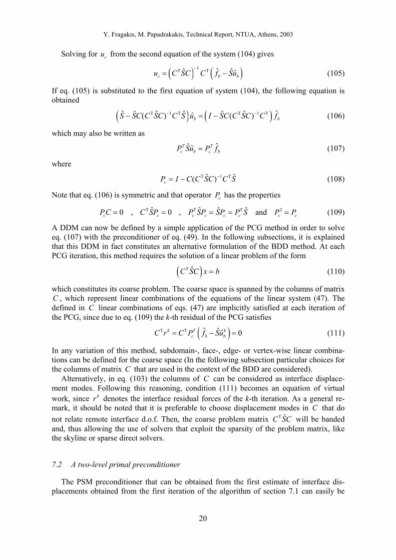
sifies the discussed methods, according to their coarse problems. Note that each row of Fig. 2 refers to methods that share the same coarse problem. Additionally, the first column of Fig. 2 contains methods in which the coarse problem is incorporated in the linear equa-tion solved by PCG, while in the methods of the second column the coarse problem is in-cluded in the preconditioner.

7.3 Connection between the two-level primal formulations

With the preconditioner of eq. (119), the standard BDD algorithm (section 7.2) has practically the same computational cost per PCG iteration as the algorithm of section 7.1. It can further be shown that these two algorithms have the same iteration count as well. This can easily be proven if one goes through the steps of the PCG method, while monitoring the relations of the PCG variables that pertain to each of the two algorithms. One is thus led to the conclusion that the the standard BDD algorithm with the initial vector of eq. (116) and its alternative that has been described in section 7.1 produce the same estimate for the interface displacement field u of the structure at each iteration. This proof is here described for the case where no reorthogonalization is used, while it can easily be deduced that all relations that are proven between the variables of the two methods also hold in the case where reorthogonalization of the direction vectors is performed. In the course of this proof, subscript is used in order to distinguish the variables of the standard BDD formu-lation from those of the formulation of section 7.1..

b

P

The variables of the PCG initialization stage can be written as: • For the algorithm of section 7.1:

, 0ˆ 0bu = ( ) 10 T T ˆˆc bu C SC C

−= f b

0 0

, (120) 0 0 ˆb c cu Cu A f= =

, and 0 ˆc br P fΤ= 0 T

b b

sp pz L S L r

+

= 0p z= (121)

• For the standard BDD algorithm:

P

0 ˆb c bu A f u0

b= = (122)

( )P

0 0P

ˆ ˆ ˆ ˆ ˆˆ ˆ ˆb b b c b c b c br f Su f SA f I SA f P f rΤ= − = − = − = = 0

0 0

(123)

and 0 T 0P b b

sc p p cz P L S L r P z

+

= = 0 0 0P P c cp z P z P p= = = (124)

In order to conclude the proof, we assume that the following relations between the vari-ables of the two algorithms hold for the k-th iteration of the PCG:

, rPb b

ˆˆk k kc b c bu u Pu A= = + f k

Pk r= , and P

kcz P z= k k

Pk

cp P p= (125)

The proof can thus be concluded by showing that the relations (125) hold for the next itera-tion : 1k +

From eqs. (125), it follows that

T T

T TP P P P

PP P P P

ˆ ˆ ˆ

k k k k k k k kk kc

k k k k k k k kc c c

z r z r z P r z rp q p Sp p P SP p p P Sp

η ηΤ Τ

Τ Τ

Τ

Τ Τ= = = = = (126)

22


Table 1

List of the discussed in this paper DDM

Name Acronym Proposed in

One-level FETI method (dual formulation) FETI-1 [FR91]

Two-level FETI method (dual formulation) FETI-2 [FM98]

Dual-primal FETI method (dual formulation) FETI-DP [FLLP+01]

Balancing Domain Decomposition method BDD [Man93]

Name AcronymLinear

equation to solve

Precon-ditioner

Primal class of FETI methods or P-FETI methods

One-level FETI method in primal formulation or one-level P-FETI method P-FETI1 (47) (79)

Two-level FETI method in primal formulation or two-level P-FETI method P-FETI2 (47) (86)

Dual-primal FETI method in primal formulation or dual-primal P-FETI method P-FETIDP (47) (90)

(127) ( )

P P

1P P

1 1

ˆˆ

ˆ ˆˆ ˆ

k k k k k k k k kb b b c c b c b c

k k k k kc b c b c b c b b

u u p u P p Pu A f P p

P u p A f Pu A f u

η η η

η

+

+ +

= + = + = + +

= + + = + =

k

kp+

1k+=

(128) 1

P P P P P P P

1

ˆ ˆ

ˆ

k k k k k k k k kc

k k k k k k kc

r r q r Sp r SP

r P Sp r q r

η η η

η η

+

Τ

= − = − = −

= − = − =

(129) 1 T 1 T 1P Pb b b b

k s k s kc p p c p p cz P L S L r P L S L r P z

+ ++ + += =

1 1 1 11 1 1P P

P P PP P

1 11 1

k k k kk k k k c

c ck k k kc

k kk k k

c ck k

z r z P r kp z p P zz r z P r

z rP z p P pz r

Τ Τ

Τ Τ Τ Τ

Τ

Τ Τ

+ + + Τ ++ + +

Τ

+ ++ +

= + = +

= + =

P p

(130)

Eq. (130) concludes recursively this proof. It is therefore clear that the two formulations are equivalent

23


FETI-1

FETI-DP

FETI-2 P-FETI2

P-FETI1

BDD(A) BDD(B)

P-FETIDP

One-level FETIcoarse problem

Two-level FETIcoarse problem

Dual-primal FETIcoarse problem

Two-level primal substru-cturing coarse problem

FETIcoarse problems

Coarse problem embedded in the linear equation solved by PCG

Coarse problem embedded in the

preconditioner

BDD(A): The BDD method formulated as the PCG applied for the solution of eq. (107) with the preconditioner of eq. (49) (Section 7.1)

BDD(B): The BDD method formulated as the PCG applied for the solution of eq. (47) with the preconditioner of eq. (112) (Section 7.2)

Figure 2. A diagram of the discussed in this paper DDM

8 Connection between the Balancing Domain Decomposition Method and the FETI method

The research in both the BDD and FETI families of methods has been progressing in parallel over the last decade and both methods have been applied in several areas of Struc-tural Mechanics as well as in other fields of Computational Mechanics. Some efforts have been made in the past to interconnect the two methods, i.e. [KW01]. In this section, we first prove that the basic formulation of the BDD method [Man93] is equivalent to P-FETI1, with matrix set equal to the Dirichlet preconditioner. We then discuss the impact of this equivalence to the general comparison of BDD and FETI.

Q

In order to prove that BDD and P-FETI1 (with matrix Q set equal to the Dirichlet pre-conditioner) are equivalent, it suffices to show that their preconditioning matrices are equal. When Q is set equal to the Dirichlet preconditioner (68), operator , which is used in the formulation of the P-FETI1 preconditioner of eq. (79), becomes

bH

24


( ) ( ) ( ) ( )(( )

T

T T

T T

T T 1

1T T

1

( )

b b b b

sb b b

)s s s s s sb p p b b b b p p b b b

s sR b R b

H I B QG G QG R

I B B S B B R R B B S B B R R

I A R A R

−

−Τ Τ

−

= −

= −

= −

(131)

where ( ) ( )Tb b

s sR b p p b bA B B S B B RΤ= (132)

Using eqs. (27), (45) and setting the interface modes matrix C equal to eq. (115), we obtain

( ) ( )( ) ( )( )

( )( )( )ˆ

b b

b b

b

b

b

s sR p b b p

s sp b b p b

sp b b

s sp b b b

sp b

A I L L S I L L R

L L I S L L R

L L I S L C

L L S L S L C

L S S L C

Τ Τ

Τ Τ

Τ

Τ

= − −

= −

= −

= −

= −

b

(133)

and similarly

( )(

T T

T T

ˆ

ˆ

ˆ

b

b

s s sb R b p b

s s sb p b b

R A R L S S L C

)R L S R S L C

C SCΤ

= −

= −

=

(134)

From eqs. (133) and (134), we have

( )( )

( ) ( )( )

( )

T T

T

1

1

1

T

ˆ ˆ

ˆ

ˆ

b b

b

b b

b b

b

b

s sb p R b R b p

sp R b R

sp p b

sp p b c

sp c b c

sp c b c

H L I A R A R L

L A R A C

L L S S L C C SC C

L L S S L A

L I SA S L A

L P S L A

−

−Τ

−Τ Τ

= −

= −

= − −

= − −

= − +

= +

(135)

The P-FETI1 preconditioner of eq. (79) with Q set equal to the Dirichlet preconditioner thus becomes

(136) ( ) ( )

1 T T

T

T T

b b

b b

b b b b

sp b b p

s s sc b c p p c b c

s s s s s s s sc p p c c b b c c p b c c b p c

A L H S H L

A L S P L S L P S L A

P L S L P A L S S S L A P L S S L A A L S S L P

+

+

+ + +

−

Τ Τ

Τ Τ Τ Τ

=

= + +

= + + ++

From eq. (46) it follows that matrix satisfies the relation cA

25


( ) ( )( )

1

1

ˆ

ˆ ˆ ˆ

ˆ

s s s sc b b c c b b c c c

c

A L S S S L A A L S L A A SA

C C SC C SC C SC C

C C SC C A

+Τ Τ

− −1Τ Τ Τ

−Τ Τ

= =

=

= =

Τ

b

Τ

Τ

=

+

I.

(137)

Furthermore, from eqs. (27), (44) and (109) it follows that there is a matrix Y such that the following relations hold

(138)

( )

( ) ( )( ) ( )

( ) ( )( ) ( )

1 1

1

1

1 1

ˆ ˆ

ˆ

ˆ

ˆ ˆ 0

b b b

b b b

b b

b b b

b

s sc p b c c p b b c c p b c c c p b c

sc p b c p b p b

sc p p b b

sc p p p b b

sc p b c

P L S S L A P L I R Y L A P L L A PCY P L L A

P L L C C SC C P L L L R C SC C

P L I B B R C SC C

P L L B B R C SC C

P L R C SC C PC C SC C

+Τ Τ Τ

− −Τ Τ Τ Τ Τ Τ

−Τ Τ Τ Τ

−Τ Τ Τ Τ Τ

− −Τ Τ Τ Τ Τ

= + = + =

= =

= −

= −

= =

Finally, using eqs. (137) and (138), eq. (136) takes the form

(139) 1 T T

T

b b b b

b b

s s s s s s s sc p p c c b b c c p b c c b p c

sc p p c c

A P L S L P A L S S S L A P L S S L A A L S S L P

P L S L P A

+ + +

+

− Τ Τ Τ Τ

Τ

= + + +

= +

It therefore follows that the P-FETI1 preconditioner (79) with Q set equal to the Dirichlet preconditioner is equivalent to the BDD preconditioner (eq. (112) with C equal to eq. (115) ). Furthermore, the similarity between the eigenspectrum of FETI-1 and P-FETI1 (which has been discussed in section 6.1), combined with the equivalence between P-FETI1 (with Q equal to the Dirichlet preconditioner) and BDD, lead to the conclusion that the BDD method and the Dirichlet preconditioned FETI-1 method (with Q equal to the Dirichlet preconditioner) should have comparable CPU time counts. Indeed, the above configuration of FETI-1 and BDD appear to have comparable performance, as is later shown in section 9 where numerical tests are performed. The connection established in this section thus allows to predict the relative performance of the one-level FETI method and the basic formulation of the BDD method [Man93]. For example, in the case of highly ill-conditioned problems (where the optimal configuration of FETI-1 uses the Dirichlet preconditioner and Q equal to the Dirichlet preconditioner [BDFL+00]), the BDD method and the optimal FETI-1 con-figuration for this problem should result in comparable solution times. For less ill-conditioned problems, a similar reasoning leads to conclusions regarding the relative performance of BDD and FET

REMARK 1. This remark makes use of the equivalence between the BDD and the P-FETI1 method (with Q equal to the Dirichlet preconditioner), in order to show that like the BDD, in this particular instance of P-FETI1 it is also possible to avoid one of the two coarse problem solutions at each iteration. More precisely, in the BDD method, it is possi-ble to avoid one of the two coarse problem solutions at each iteration by setting the initial vector of interface displacements equal to eq. (116). Similarly, the choice of a vector 0

bu

26


equal to eq. (116) has the same positive effect in the P-FETI1 method with Q equal to the Dirichlet preconditioner. Note that due to eqs. (132) and (134), in the case of P-FETI1 the initial vector of eq. (116) takes the form 0

bu

T

ˆ

( ) ( )( ) ( )(

( )

T

T

T

110

1T

1

ˆ ˆˆ

ˆ

ˆb b b

b b

sb c b b b R

s s s s sp b b b p p b b b p b

s sp b b p b

u A f C C SC C f C R A C f

L R R B B S B B R R L f

L R G QG R L f

−−Τ Τ Τ

−Τ Τ

−Τ Τ

= = =

=

=

(140) ) b

b

Hence, if the initial vector of P-FETI1 is set equal to eq. (140), the residuals of P-FETI1 with Q equal to the Dirichlet preconditioner, satisfy the condition (117)

0bu

, T

0 0b

k s kb pC r R L rΤ = ⇒ = 0,1,... k = (141)

Due to eq. (141), the following holds

, b b

k kb p pH L r L r= 0,1,... k = (142)

From eq. (142), it can be deduced that with the initial vector u of eq. (140), the P-FETI1 preconditioner (79) may be implemented as follows

0b

(143) 1 T Tb

sp b pA L H S L

+− =b

where only one solution of the coarse problem is required within the preconditioning step. It is also worth noting the analogy between the P-FETI1 and FETI-1 method in this issue. In particular, as in P-FETI1, in FETI-1 it is also possible to remove the one of the two coarse problem solutions per iteration if matrix is set equal to the Dirichlet precondi-tioner [FR94].

Q

9 Numerical performance of the introduced methods

In this section, numerical tests are performed in order to compare the performance of the DDM that have been discussed in this paper. In particular, the number of iterations re-quired to reach different levels of solution accuracy, as well as the minimum achieved error are compared for the different methods. It is worth noting that each original Dirichlet pre-conditioned FETI variant discussed in this paper and its corresponding P-FETI variant have a similar computational cost in both the initialization phase and at each iteration. In-deed, they require the solution of the same local subdomain and coarse space problems at each iteration. Only small differences in the CPU time of each iteration appear, like for example in the computational costs related to the reorthogonalization of the direction vec-tors. In original FETI methods the dimension of the direction vectors is equal to the num-ber of Lagrange multipliers, while in P-FETI methods their dimension is equal to the num-ber of interface d.o.f., which is typically smaller than the number of Lagrange multipliers in the presence of cross-points, particularly in 3-D elasticity problems and in the case of redundant Lagrange multipliers. However, such differences are relatively small. Therefore, in order to estimate which method is actually faster, it suffices to compare the iteration counts required for convergence.

Furthermore, it is worth investigating the solution precision that can be achieved by the discussed methods. In fact, DDM have repeatedly been used in the past to solve highly

27


large-scale and ill-conditioned problems. It is thus important to investigate the conver-gence capabilities of the methods, in highly ill-conditioned problems. Therefore, the dis-cussed DDM are also compared in this section in terms of the level of solution accuracy that can be achieved.

In order to compare the iteration counts and the minimum attainable error of the meth-ods, we have run a number of test cases using a research code that has been developed for that purpose on the Matlab computing environment. In order to compute accurately the iteration counts and minimum residual, this code simulates the state of the art techniques used to implement the discussed DDM in FORTRAN, C or C++ programming languages for high performance applications (see for example the FETI implementation discussion in [FPL00]). Hence, in the subsequently presented results, unless otherwise specified, the DDM are implemented as follows: • All methods are implemented with reorthogonalization of the direction vectors. • In FETI-1 and FETI-2 methods, we employ the algorithms that are derived after us-

ing the transformations of eqs. (67). Furthermore, the FETI-2 coarse problem matrix that is related to the cross-points is formed using the formulation presented in [FPL00].

• It was found in a number of tests performed by the authors, that the choice of any of the three different definitions of Lagrange multipliers practically does not affect the convergence history of original FETI and P-FETI variants. Therefore, in the results presented in this section, redundant Lagrange multipliers are used for FETI-1, while non-redundant multipliers are used for the FETI-2 runs, in order to minimize the di-mension of the FETI-2 coarse problem which is related to the cross-point Lagrange multipliers.

• The local subdomain problems of the implemented DDM are usually solved using the direct skyline solver. The Choleski factorization method is thus used in the per-formed tests with optimal node renumbering for skyline solvers. In addition, the zero energy modes and artificial constraints of semi-definite subdomain problems are ob-tained with the geometric-algebraic method presented in [PF01].

• In order to use the same convergence criterion for the different methods, conver-gence is monitored with the criterion:

f Ku f ε− < (144)

where ε is the convergence threshold parameter. Therefore, even though the dis-cussed DDM require computing a full displacement field estimate only after conver-gence, it is computed here at each iteration in order to obtain the residual quotient of eq. (144).

• A Pentium IV processor at 1.7 GHz has been used in the test runs.

9.1 A 3-D elasticity test problem

The 3-D elasticity problem of Fig. 3 is used as the first test problem. The cubic structure of Fig. 3 is composed of five layers of two different materials and is discretized with

8-node brick elements. Additionally, it is pinned at the four corners of its left surface and is subjected to gravity load. An optimal decomposition of this heterogeneous problem must generate subdomains with good aspect ratios, while preserving the material interfaces when partitioning the model [BDFL

28 28 28× ×

+00]. Hence, two decompositions of this het-erogeneous model of 73 d.o.f. in 100 subdomains, obtained with TOPDOMDEC [SF94], are considered: In the first decomposition (Fig. 4a), the model has been partitioned

,155

28


in subdomains with good aspect ratios without taking into account the material interfaces (Decomposition P1). In the second decomposition (Fig. 4b), the five layers of different materials have been partitioned independently, thus generating a decomposition which pre-serves the material interfaces but produces subdomains of suboptimal aspect ratio in the thin layers (Decomposition P2).

The number of iterations required to reach different levels of solution accuracy and the maximum accuracy achieved by FETI-1 and P-FETI1 methods in this 3-D elasticity prob-lem are presented in Table 2. Different ratios A BE E of the Young moduli of the two ma-terials are considered, while their Poisson ratio is set equal to A B 0.30ν ν= = . Table 2 thus presents the results obtained for homogeneous material properties using partitioning P1 and for heterogeneous material properties using either partitioning P1 or P2. In the homo-geneous case, matrix Q is set equal to the unit matrix and homogeneous scaling is used, while in the heterogeneous case, the methods are implemented with heterogeneous scaling and Q is set equal to the superlumped matrix . SLQ

The choice of the superlumped matrix is optimal for this problem, since the choices of DQ Q= or have been found not to improve significantly the iteration count of the

methods, while they entail more computational cost in the initialisation and in each itera-tion of the methods.

LQ Q=

From the results of Table 2, it follows that in the homogeneous case P-FETI1 has the same iteration count as the FETI-1 method with the Dirichlet preconditioner. In the hetero-geneous cases however, the P-FETI1 method performs 2-8% less iterations than the Dirichlet preconditioned FETI-1 method. It should be noted that decomposition P2 leads to less iterations than decomposition P1. Moreover, in the heterogeneous cases P-FETI1 achieves higher solution accuracy than FETI-1. In particular, the minimum errors of P-FETI1 and FETI-1 methods differ by one-half to one order of magnitude.

Figure 3. A cubic structure composed of two materials

29


(a) (b)

Figure 4. Two decompositions of the cubic test problem in 100 subdomains: (a) Optimal aspect ratio partitioning (Decomposition P1),

(b) Layered partitioning (Decomposition P2)

Similar results have also been observed in other 2-D and 3-D elasticity tests performed by the authors. More precisely, in most of the tests performed in homogeneous problems, P-FETI and original FETI methods with the Dirichlet preconditioner have the same itera-tion counts. However, in the heterogeneous test cases and in some homogeneous ones, P-FETI variants give smaller number of iterations than the Dirichlet preconditioned FETI variants with dual formulation. Additionally, even though P-FETI and original FETI meth-

Table 2

Number of iterations and maximum attained precision achieved by FETI-1 and P-FETI1 methods for the 3-D elasticity test problem

Type of method FETI-1 Lumped preconditioner

FETI-1 Dirichlet preconditioner P-FETI1

Tolerance and minimum error 10-5 10-7 10-9 Min.

error 10-5 10-7 10-9 Min. error 10-5 10-7 10-9 Min.

error

A BE E Decom-position

100 P1 32 39 47 2.1·10-10 27 33 39 2.6·10-10 27 33 39 5.2·10-11

P1 56 67 79 8.4·10-10 41 49 59 9.1·10-10 39 48 56 5.1·10-10

103 P2 33 40 – 1.1·10-9 27 32 – 1.2·10-9 26 31 37 4.8·10-10

P1 63 – – 4.0·10-6 48 – – 3.6·10-6 44 – – 4.7·10-7

106 P2 37 – – 5.0·10-6 31 – – 5.4·10-6 29 – – 4.3·10-7

30


ods reach approximately the same minimum error in some of the tests performed on het-erogeneous problems, in most tests P-FETI methods achieve higher solution accuracy than the original FETI methods.

9.2 A semi-cylindrical panel problem

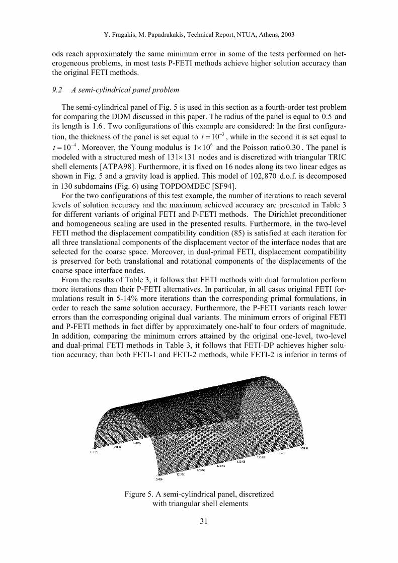
The semi-cylindrical panel of Fig. 5 is used in this section as a fourth-order test problem for comparing the DDM discussed in this paper. The radius of the panel is equal to 0.5 and its length is 1.6 . Two configurations of this example are considered: In the first configura-tion, the thickness of the panel is set equal to t 310−=

60×, while in the second it is set equal to

. Moreover, the Young modulus is 1 1 and the Poisson ratio . The panel is modeled with a structured mesh of 131

410t −= 0.30131× nodes and is discretized with triangular TRIC

shell elements [ATPA98]. Furthermore, it is fixed on 16 nodes along its two linear edges as shown in Fig. 5 and a gravity load is applied. This model of 102 d.o.f. is decomposed in 130 subdomains (Fig. 6) using TOPDOMDEC [SF94].

,870

For the two configurations of this test example, the number of iterations to reach several levels of solution accuracy and the maximum achieved accuracy are presented in Table 3 for different variants of original FETI and P-FETI methods. The Dirichlet preconditioner and homogeneous scaling are used in the presented results. Furthermore, in the two-level FETI method the displacement compatibility condition (85) is satisfied at each iteration for all three translational components of the displacement vector of the interface nodes that are selected for the coarse space. Moreover, in dual-primal FETI, displacement compatibility is preserved for both translational and rotational components of the displacements of the coarse space interface nodes.

From the results of Table 3, it follows that FETI methods with dual formulation perform more iterations than their P-FETI alternatives. In particular, in all cases original FETI for-mulations result in 5-14% more iterations than the corresponding primal formulations, in order to reach the same solution accuracy. Furthermore, the P-FETI variants reach lower errors than the corresponding original dual variants. The minimum errors of original FETI and P-FETI methods in fact differ by approximately one-half to four orders of magnitude. In addition, comparing the minimum errors attained by the original one-level, two-level and dual-primal FETI methods in Table 3, it follows that FETI-DP achieves higher solu-tion accuracy, than both FETI-1 and FETI-2 methods, while FETI-2 is inferior in terms of

Figure 5. A semi-cylindrical panel, discretized

with triangular shell elements

31


Figure 6. A decomposition of the semi-cylindrical

panel in 130 subdomains – Top view

solution accuracy than the three variant FETI methods. However, the respective P-FETI variants reach approximately the same solution precision.

It should be further noted that in a number of plate and shell problems tested by the au-thors, a similar reduction in iteration counts and minimum errors has been observed for the P-FETI formulations. More precisely, in all tests performed in fourth-order problems, P-FETI methods give less iterations than the corresponding FETI methods with dual formula-tion. Furthermore, even though in a few of the performed tests the two formulations achieve almost the same maximum solution accuracy, in most of the tests performed so far, P-FETI configurations attain higher solution precision. Thus, the P-FETI methods appear capable of providing more accurate solutions in a number of ill-conditioned plate and shell problems.

The differences that typically appear in the convergence history of original FETI and P-FETI methods in fourth-order problems are depicted in Fig. 7, which illustrates the solu-tion accuracy versus the number of iterations of FETI-1 and P-FETI1 methods, for the semi-cylindrical panel problem. In Fig. 7 it can be observed that the value of the FETI-1 initial error is high, compared to the value of the P-FETI1 initial error which lies in the vicinity of 1. After a number of iterations, the convergence curves of the two methods be-come almost parallel, while the P-FETI1 error remains always lower than the FETI-1 error. Finally, FETI-1 stagnates at a higher level than P-FETI1. The above mentioned differences

Figure 7. Error quotient of eq.(144) versus number of iterations for FETI-1 and P-

FETI1 methods with Q for the semi-cylindrical panel with t = 10I= -3

32


are typically observed when comparing the dual and the corresponding primal methods in fourth-order or heterogeneous second-order problems, while in homogeneous second-order problems, the convergence curves of original FETI methods and their P-FETI alternatives typically coincide after a number of initial iterations and finally stagnate at approximately the same solution error.

Moreover, it can be seen from Table 3 that in FETI-1 and P-FETI1 methods setting ma-trix equal to the superlumped choice (Q Q ) or equal to the Dirichlet preconditioner, results in a substantial reduction of the iteration counts, compared to the choice of

Q SL=Q I= .

In particular, both P-FETI1 and FETI-1 with Q set equal to the Dirichlet preconditioner perform 58-63% less iterations than when choosing Q I= . A similar reduction in FETI-1 iteration counts has also been observed in fourth-order problems by Rixen [Rix00]. Based on these remarks, it follows that setting Q I≠ can substantially improve the computational time required by FETI-1 and P-FETI1 methods, for the solution of plate and shell prob-lems. It is also worth noting that the results reported in Table 3 for P-FETI1 with DQ Q=

Q

, are practically the same as those that we have obtained for the standard BDD method [Man93], due to the equivalence between this configuration of the P-FETI1 method and the BDD method. Moreover, it should be noted that in FETI-1 and P-FETI1 methods with set equal to the Dirichlet preconditioner, when omitting the one of the two coarse problem solutions per iteration, a decrease in the maximum achieved solution accuracy is observed. In particular, Table 3 shows that a decrease of one-half to almost three orders of magnitude to the maximum accuracy is caused by skipping the one coarse solution at each iteration.

33

Table 3

Number of iterations and maximum precision of original FETI and P-FETI methods for the two configurations of the semi-cylindrical panel

Panel thickness t = 10-3 t = 10-4

Original FETI / P-FETI Formulations Original FETI P-FETI Original FETI P-FETI

Tolerance and minimum error 10-2 10-4 10-6 Min.

error 10-2 10-4 10-6 Min. error 10-2 10-3 10-4 Min.

error 10-2 10-3 10-4 Min. error

Type of method

Q = I 341 372 – 6.9·10-6 318 354 385 7.9·10-8 >500 >500

Q = QSL 197 224 – 6.0·10-6 181 212 237 7.0·10-8 424 – – 1.7·10-3 395 408 425 7.1·10-5

Q = QD – two coarse problem solutions per iteration 132 156 – 6.7·10-6 118 144 169 4.6·10-8 330 – – 1.9·10-3 297 319 340 6.1·10-5

One

-leve

l FET

I

Q = QD – one coarse problem solution per iteration 132 159 – 3.6·10-5 118 144 169 1.7·10-7 – – – 9.5·10-1 297 319 – 2.4·10-4

Coarse problem related only to cross-points 43 54 – 1.1·10-5 38 50 61 1.8·10-8 – – – 2.1·10-1 99 111 123 2.7·10-5

TFwo-

leve

l ET

I

Coarse problem related to cross-points and ends of interface edges 34 44 – 1.1·10-5 30 40 51 1.5·10-8 – – – 9.7·10-2 80 91 102 1.7·10-5

Coarse problem related only to cross-points 72 86 101 2.7·10-7 64 80 94 4.2·10-8 186 202 – 4.4·10-4 165 180 196 2.8·10-5

Dua

l-prim

al

FETI

Coarse problem related to cross-points and ends of interface edges 46 59 71 1.1·10-7 41 54 66 6.3·10-8 142 157 – 1.5·10-4 125 139 153 4.2·10-5


10 Summary and concluding remarks

In this paper novel Domain Decomposition Methods (DDM) are introduced, while pre-viously known DDM are classified using a unified framework for primal and dual DDM. The developed framework is independent from the choice of homogeneous or heterogene-ous scaling and the definition of the Lagrange multipliers.

Moreover, a new class of methods (P-FETI class of methods) is proposed based on the respective existing FETI variants. Furthermore, the introduced P-FETI methods are shown to be closely related to the original FETI variants. In particular, the one-level FETI method (FETI-1) has a similar eigenspectrum as the corresponding P-FETI method (P-FETI1). This finding and the similarity in the way different P-FETI methods are formulated from the original FETI methods, lead to the conclusion that there probably exist theoretical con-nections, similar to those between P-FETI1 and FETI-1, for the other FETI variants. Fur-thermore, two alternative formulations of the Balancing Domain Decomposition method (BDD) are described, while a connection between the BDD and FETI methods is estab-lished.

Additionally, the computational efficiency of the P-FETI methods is compared with the corresponding original FETI methods in a number of numerical tests. The obtained results show that in homogeneous second-order problems the previously known Dirichlet precon-ditioned FETI methods and the respective P-FETI variants have approximately the same computational cost. In fourth-order and heterogeneous second-order problems, however, the original FETI methods with the Dirichlet preconditioner are typically slower than the corresponding P-FETI configurations. Furthermore, the P-FETI methods typically attain higher solution accuracy in these problems, as well. They thus provide a more robust cate-gory of methods for solving ill-conditioned fourth-order and heterogeneous second-order problems. In general, the introduced P-FETI methods retain the thoroughly investigated in the past years optimal convergence properties of the FETI method, while they appear ca-pable of providing faster and more accurate solutions in a number of problems.

In addition, general remarks drawn from the present study may be summarized to the following. It is well known that each DDM is basically characterized by the quality of its coarse problem. The importance of the coarse space leads to a classification of the existing and introduced methods according to the type of coarse problem employed and its position in the method’s formulation. The thus obtained classification is schematically depicted in Fig. 2. This figure shows that for each coarse problem, two formulations can be obtained, placing the coarse problem either in the linear problem solved by the PCG or in the pre-conditioner. The two formulations lead to methods with either similar or different theoreti-cal and numerical properties, depending on the type of problem at hand, as is shown in the sections of this paper.

Acknowledgements

The authors would like to thank Dimos Charmpis for developing a part of the Matlab DDM code employed in this paper. The first author would further like to thank his collaborators Sotiris Bitzarakis, Constantina Apostolopoulou and George Stavroulakis, for their advice and help in issues regarding the FETI method. Finally, this work is partially supported by the research project “Archimedes” of the National Technical University of Athens.

35


36

References

[ATPA98] J. Argyris, L. Tenek, M. Papadrakakis, C. Apostolopoulou, Postbuckling performance of the TRIC natural mode triangular shell element for isotropic and laminated composite shells, Comput. Methods Appl. Mech. Engrg., 166, 211-231 (1998)

[BPK97] S. Bitzarakis, M. Papadrakakis, A. Kotsopoulos, Parallel solution techniques in computational structural mechanics, Comput. Methods Appl. Mech. Engrg., 148, 75-104 (1997)

[BDFL+00] M. Bhardwaj, D. Day, C. Farhat, M. Lesoinne, K. Pierson, D. Rixen. Applica-tion of the FETI Method to ASCI Problems: Scalability results on one-thousand proces-sors and discussion of highly heterogeneous problems. Int. J. Numer. Meth. Engng., 47, 513-536 (2000)

[CP02] D. C. Charmpis, M. Papadrakakis, Enhancing the performance of the FETI method with preconditioning techniques implemented on clusters of networked computers, Com-putational Mechanics, 30, 12-28 (2002)

[FCMR98] C. Farhat, P. S. Chen, J. Mandel, F. X. Roux, The two-level FETI method – part II: extension to shell problems, parallel implementation and performance results, Comput. Methods Appl. Mech. Engrg., 155, 153-180 (1998)

[FCRR98] C. Farhat, P.-S. Chen, F. Risler, F. X, Roux, A unified framework for accelerat-ing the convergence of iterative substructuring methods with Lagrange multipliers, Int. J. Numer. Meth. Engng., 42, 257-288 (1998)

[FLLP+01] C. Farhat, M. Lesoinne, P. LeTallec, K. Pierson, D. Rixen, FETI-DP : A dual-primal unified FETI method – part I: A faster alternative to the two-level FETI method, Int. J. Numer. Meth. Engng., 50, 1523-1544 (2001)

[FLP00] C. Farhat, M. Lesoinne, K. Pierson, A scalable dual-primal domain decomposition method, Numer. Lin. Alg. Appl., 7(7-8), 687-714 (2000)

[FM98] C. Farhat, J. Mandel, The two-level FETI method for static and dynamic plate problems – part I: an optimal iterative solver for biharmonic systems, Comput. Methods Appl. Mech. Engrg., 155, 129-152 (1998)

[FMR94] C. Farhat, J. Mandel, F.-X. Roux, Optimal convergence properties of the FETI domain decomposition method, Comput. Methods Appl. Mech. Engrg. 115, 365-385 (1994)

[FPL00] C. Farhat, K. Pierson and M. Lesoinne. The second generation FETI methods and their application to the parallel solution of large-scale linear and geometrically non-linear structural analysis problems. Comput. Methods Appl. Mech. Engrg., 184, 333-374 (2000)

[FR91] C. Farhat, F.-X. Roux, A method of finite element and interconnecting and its par-allel solution algorithm, Int. J. Numer. Meth. Engng., 32, 1205-1227 (1991)

[FR94] C. Farhat, F.-X. Roux, Implicit parallel processing in structural mechanics, Com-put. Mech. Adv., 2, 1-124 (1994)

[FP02a] Y. Fragakis, M. Papadrakakis, A unified framework for formulating Domain De-composition Methods in Structural Mechanics, Technical Report, National Technical University of Athens, Greece, March 2002, http://users.ntua.gr/fragayan


37

[FP02b] Y. Fragakis, M. Papadrakakis, A Family of New FETI Methods for Structural Mechanics, Proceedings of the Fifth World Congress on Computational Mechanics (WCCM V), Vienna, Austria, July 7-12, 2002, http://wccm.tuwien.ac.at

[JPF97] M. R. Justino Jr, K. C. Park, and C. A. Felippa, An algebraically partitioned FETI method for parallel structural analysis: Implementation and numerical performance evaluation, Int. J. Numer. Meth. Engng., 40, 2739–2758 (1997)

[KW01] A. Klawonn, O. B. Widlund, FETI and Neumann-Neumann iterative substructur-ing methods: connection and new results, Communications on pure and applied Mathe-matics, 54, 57-90 (2001)

[LMV98] P. LeTallec, J. Mandel, M. Vidrascu, A Neumann--Neumann Domain Decompo-sition Algorithm for Solving Plate and Shell Problems, SIAM J. Numer. Anal., 35, 836-867, (1998)

[LV97] P. LeTallec, M. Vidrascu, Solving large scale structural problems on parallel com-puters using Domain Decomposition techniques, in M. Papadrakakis (Ed.), Parallel solu-tion methods in Computational Mechanics, John Wiley & Sons, New York, (1997)

[Man93] J. Mandel, Balancing domain decomposition, Commun. Appl. Numer. Meth., 9, 233-241 (1993)

[PF01] M. Papadrakakis, Y. Fragakis, An integrated geometric-algebraic method for solv-ing semi-definite problems in Structural Mechanics, Comput. Methods Appl. Mech. Engrg., 190 (49-50), 6513-6532 (2001)

[PJF97] K. C. Park, M. R. Justino Jr., C. A. Felippa, An algebraically partitioned FETI method for parallel structural analysis: Algorithm description, Int. J. Numer. Meth. Engng., 40, 2717-2737 (1997)

[Rix00] D. Rixen, Choosing the coarse grid when applying FETI to heterogeneous struc-tures, Presentation at the 13th International Conference on Domain Decomposition Meth-ods, Lyon, France, October 9-12, 2000

[RF99] D. Rixen, C. Farhat, A simple and efficient extension of a class of substructure based preconditioners to heterogeneous structural mechanics problems, Int. J. Numer. Meth. Engng., 44 (4), 489-516 (1999)

[RFTM99] D. Rixen, C. Farhat, R. Tezaur, J. Mandel, Theoretical comparison of the FETI and algebraically partitioned FETI methods, and performance comparisons with a direct sparse solver, Int. J. Numer. Meth. Engng., International, 46, 501-534 (1999)

[SF94] M. Sharp and C. Farhat. TOPDOMDEC – A totally object oriented program for visualization, domain decomposition and parallel processing. User’s manual, PGSoft and University of Colorado, Boulder, USA, (1994)

The mosaic of high performance Domain …€¦The mosaic of high performance Domain Decomposition...

Documents

Transcript of The mosaic of high performance Domain …€¦The mosaic of high performance Domain Decomposition...