The More the Merrier? The Effect of Family Size and...
50
The More the Merrier? The Effect of Family Size and Birth Order on Children’s Education Sandra Black Paul Devereux Kjell Salvanes June 2005
Transcript of The More the Merrier? The Effect of Family Size and...
The More the Merrier? The Effect of Family Size
and Birth Order on Children’s Education
Sandra Black
Paul Devereux
Kjell Salvanes
June 2005
Published by
Centre for the Economics of Education
London School of Economics
Houghton Street
London WC2A 2AE
© Sandra Black, Paul Devereux and Kjell Salvanes, submitted March 2005
ISBN 07530 1846 2
Individual copy price: £5
The Centre for the Economics of Education is an independent research centre funded by the Department for Education and Skills. The views expressed in this work are those of the author and do not reflect the views of the DfES. All errors and omissions remain the authors. This paper was presented as part of the Centre for the Economics of Education seminar series on 25th February 2005.

Abstract
There is an extensive theoretical literature that postulates a trade off between child
quantity and quality within a family. However, there is little causal evidence that speaks
to this theory. Using a rich dataset on the entire population of Norway over an extended
period of time, we examine the effects of family size and birth order on the educational
attainment of children. While we find a negative correlation between family size and
children's education, when we include indicators for birth order and/or use twin births as
an instrument, family size effects become negligible. In addition, birth order has a
significant and large negative effect on children's education. We also study adult
earnings, employment, and teenage childbearing, and find strong evidence for birth order
effects with these outcomes, particularly among women. These findings suggest the need
to revisit economic models of fertility and child "production", focusing not only on
differences across families but differences within families as well.


The More the Merrier? The Effect of Family Size
and Birth Order on Children’s Education
Sandra Black
Paul Devereux
Kjell Salvanes
1. Introduction 1
2. Data 4
Relevant institutional detail 5
3. Family Size 6
Regression results 9
Controlling for family background characteristics 10
Controlling for birth order 11
Using twins as an instrument for family size 11
Validity of twins instrument 13
Results using twins 14
Using same sex as an instrument for family size 15
4. Birth Order 16
Birth order results 18
5. Heterogeneous Effects of Family Size and Birth Order 19
6. Other Outcomes 21
Labour market outcomes 22
Probability of having a teen birth 24
7. Conclusions 25
References 28
Tables 31
Figures 42

Acknowledgments
The authors would like to thank Daron Acemoglu, Janet Currie, Mary Daly, Kanika
Kapur, Paul Schultz, and participants at the Society of Labour Economists 2004 Annual
Meetings, the Federal Reserve Bank of San Francisco, the 2004 IRP Summer Institute,
Dartmouth College, Texas A&M, University of Houston, University College Dublin,
ESSLE 2004, Humbolt University, Aarhus Business School, the NBER Labour Studies
Group, and the 2005 Winter Meetings of the Econometric Society for helpful comments.
Black and Devereux gratefully acknowledge financial support from the National Science
Foundation and the California Centre for Population Research.
Sandra Black is Assistant Professor in Economics at the University of California at Los
Angeles (UCLA) and a Research Fellow at the Institute of Labour Economics (IZA) and
the National Bureau of Economic Research. Paul Devereux is an Assistant Professor in
Economics at UCLA, and Research Fellow at IZA, and Kjell Salvanes is Professor of
Economics at the Norwegian School of Economics and Business Administration, and a
Research Fellow at Statistics Norway and IZA.

1. Introduction
Economists have long been interested in understanding the factors that determine
child outcomes. However, despite years of research, evidence on the components of the
“production function” for children is still quite limited. Family environment is widely
believed to be a primary component, but it is difficult to parcel this out into specific
characteristics.
Among the perceived inputs in the production of child quality is family size.
Greater family size may negatively affect child outcomes through resource dilution or
because the average maturity level in the household is lower. One could also imagine a
positive relationship between family size and child quality if children stabilize marriages
or decrease the probability that both parents work outside the home.
One popular economic model is the quantity-quality model introduced by Becker
[1960] and expanded in Becker and Lewis [1973]; this theory was introduced to explain
the observed negative correlation between family income and family size; it is often cited
and is used as the basis for many macro growth models.1 A key element of the quantity-
quality model is an interaction between quantity and quality in the budget constraint that
leads to rising marginal costs of quality with respect to family size; this generates a
tradeoff between quality and quantity.2 But is this tradeoff real? Casual evidence
suggests children from larger families have lower average education levels. However, is
it true that having a larger family has a causal effect on the “quality” of the children? Or
1 See Becker and Barro [1988] and Doepke [2003]. 2 Rosenzweig and Wolpin [1980] explicitly derive the assumptions under which an exogenous increase in family size should have a negative effect on child quality. They, like Becker and Lewis, treat quality as unvarying within a family.
2
is it the case that families who choose to have more children are (inherently) different,
and the children would have lower education regardless of family size?
This paper first attempts to isolate the causal effect of family size on children’s
outcomes by using data on the entire population of Norway and looking at the effect of an
exogenous increase in the size of a family on children’s educational attainment. Our
dataset includes several labor market outcomes in addition to education, covers an
extended period of time, and allows us to match adult children to their parents and
siblings; as a result, we are able to overcome many limitations of earlier research
resulting from small sample sizes or limited information on children’s outcomes after the
children have left home. In addition, we have plausibly exogenous variation in family
size (induced by the birth of twins) to identify the causal effect.
Like most previous studies, we find a negative correlation between family size
and children’s educational attainment. However, when we include indicators for birth
order, the effects of family size are reduced to almost zero. These results are robust to a
number of specifications, including the use of twins as an instrumental variable for family
size. The evidence suggests that family size itself has little impact on the quality of each
child but more likely impacts only the marginal children through the effect of birth order.
The implications of these findings are quite different from the causal effect of family size
on child quality implied by the simple quality/quantity model and may suggest a
reconsideration of the determinants of child outcomes.
Given that birth order effects appear to drive the observed negative relationship
between family size and child education, we next turn our attention to birth order. There
are a number of theories that can predict birth order effects; among these are optimal

3
stopping models, physiological differences, and dilution of parental resources when
young (both financial and time). Previously, birth order effects have proven very
difficult to credibly estimate due to rigorous data requirements [Blake, 1989]. Our unique
dataset allows us to overcome these data problems; unlike the previous literature, we are
able to look both across families and within families using family fixed effects models to
deal with unobserved family-level heterogeneity. We find that birth order effects are
strong, regardless of our estimation strategy. Moreover, the effects appear to be of
similar magnitude across families of different sizes.
We augment the education results by using earnings, full-time employment status,
and whether the individual had a birth as a teenager (among women) as additional
outcome variables. Consistent with our earlier findings, we find little support for
significant family size effects and strong evidence for birth order effects with these
outcomes, particularly for women. Later-born women have lower earnings (whether
employed full-time or not), are less likely to work full-time, and are more likely to have
their first birth as a teenager. In contrast, while later-born men have lower full-time
earnings, they are not less likely to work full-time.
The paper unfolds as follows. Section 2 describes our data. Section 3 describes
the empirical literature on the effects of family size and then presents our methodology
and results. Section 4 describes our birth order results. Section 5 presents family size and
birth order estimates for various subgroups of the sample. Section 6 presents results for
other outcomes such as earnings, employment, and teenage pregnancy. Finally, Section 7
concludes.

4
2. Data
Our data are from matched administrative files that cover the entire population of
Norway who were aged 16-74 at some point during the 1986 to 2000 interval.3 To be
included in our sample, parents must appear in this dataset in at least one year, so we do
not observe any parents older than 74 in 1986. The data also contain identifiers that allow
us to match these individuals to their children, who also must appear in the administrative
dataset at least once in the 1986-2000 period.4 We restrict our sample to children who
are at least 25 years of age in 2000 to ensure that almost all have completed their
education.5 Given that we observe year of birth, we are able to construct indicators for the
birth order of each child. Data on twin status is also available from Statistics Norway.
We use twins to construct our instrumental variables but drop twins from our estimating
samples.6 A twin birth occurs in approximately 1.5 percent of families.
Our family size measure is completed family size. We have two sources of this
information: we have data on both the total number of children born to each mother
(from the Families and Demographics file from Statistics Norway) as well as a count of
the number of children who are sixteen or over in the 1986-2000 interval. These numbers
agree in 84 percent of cases. The primary reason for disagreement is families with
children who are too young to be in the 1986-2000 data (14 percent of cases). We restrict
3 The documentation for these data is available in Møen, Salvanes and Sørensen [2004]. 4 When matching children to parents, we match using the mother’s identifier, as almost all children over this period would have grown up with their mother. However, for a small proportion of children (2 percent) the father differs across children in the family, and for a larger proportion (16 percent) the father of some of the children is unknown to Statistics Norway (so the father may be different across children). We have verified that all results are robust to excluding families in which the father identifier differs across children or is missing for some children. 5 Only 4.6 percent of our sample is still in school in 2000. As a check on this censoring problem, we have re-estimated all specifications using a sample of individuals aged at least 30 in 2000 and found very similar results.

5
our sample to families in which the mother and all children are alive and observed in our
data at some point between 1986 and 2000. By doing this, we exclude families with
children younger than 16 in 2000. This makes it fairly certain that we have completed
family size, as it is unlikely that a child of 25 who has no siblings aged less than 16 will
subsequently have another sibling. Also, it allows us to accurately calculate birth order
and the spacing measures we use. We also exclude a small number of families in which a
birth is reported as occurring before the mother was 16 or after the mother was 49.
Educational attainment is reported annually by the educational establishment
directly to Statistics Norway, thereby minimizing any measurement error due to
misreporting. The education register started in 1970; we use information from the 1970
Census for individuals who completed their education before then. Thus, the register data
are used for all but the earliest cohorts of children who did not get any additional
education after 1970. Census data are self reported but the information is considered to be
very accurate; there are no spikes or changes in the education data from the early to the
later cohorts. We drop the small number of children who have missing education data
(0.8 percent of cases).
Table I presents summary statistics for our sample and Table II shows the
distribution of family sizes in our sample. About 18 percent of families have one child,
41 percent have 2, 27 percent have 3, 10 percent have 4, and about 5 percent have 5 or
more.
2.1 Relevant institutional detail
6 Results were not sensitive to this exclusion. We dropped twins because of the ambiguities involved in defining birth order for twins.

6
The Norwegian education system has long been publicly provided and free to all
individuals. In 1959, the Norwegian Parliament legislated a mandatory school reform
that was implemented between 1959 and 1972 with the goal of both increasing
compulsory schooling (from 7 to 9 years) and to standardize access and curriculum
across regions. In 1997 compulsory schooling was increased to 10 years by reducing the
school start age from 7 to 6. Education continues to be free through college. Levels and
patterns of educational attainment in Norway are similar to those in the United States. As
can be seen in Table III, about 39 percent of children in our sample complete less than 12
years of schooling, 29 percent complete exactly 12 years, and 32 percent complete more
than 12 years. In Norway, many students engage in education that is vocational in nature
in lieu of a more academic high school track. We treat all years of education equally in
measuring education.7
The birth control pill was introduced in Norway in the late 1960s and so was
unavailable to most cohorts of parents in the sample we study [Noack and Ostby, 1981].
Abortion was not legalized in Norway until 1979 so was not relevant to any of the
cohorts we study. Government-provided daycare did not begin until the 1970s and so was
only available to the later cohorts of children in our sample.8
3. Family Size
The empirical literature on the effects of family size on child outcomes generally
supports a negative relationship between family size and child “quality” (usually
7 See Aakvik, Salvanes and Vaage [2004] for a useful description of the Norwegian educational system. 8 Later in the paper, we compare the relationship between family size and education for earlier and later cohorts to see if it changed due to these institutional differences.

7
education), even after controlling for socio-economic factors.9 However, few of these
findings can be interpreted as causal; family size is endogenously chosen by parents and
hence may be related to other unobservable parental characteristics that affect child
outcomes.
In addition to the issues of endogeneity, the literature suffers from significant data
limitations. Typically the studies do not have large representative datasets and do not
study outcomes of economic interest, such as completed education and earnings.
Additionally, the absence of information on birth order often means that birth order
effects are confounded with family size effects. While the literature is extensive, we
discuss below some of the studies that attempt to deal with some or all of these problems.
Rosenzweig and Wolpin [1980], Lee [2003], and Conley [2004] all attempt to use
exogenous variation in family size to determine the causal relationship between family
size and child “quality”. 10 Rosenzweig and Wolpin [1980], using data from India, and
Lee [2003], using data from Korea, examine the effect of increases in fertility induced by
twin births and sex of the first child, respectively, on child quality. Rosenzweig and
Wolpin find that increases in fertility decrease child quality, while Lee finds that, if
anything, larger families result in more educational expenditures per child. However, in
both cases the sample sizes are small (25 twin pairs for Rosenzweig and Wolpin,
approximately 2000 families for Lee), the estimates imprecise, and any family size effect
could be confounded by the omission of birth order controls.
In one of the most thorough studies to date, Conley [2004] uses U.S. Census data
from 1980 and 1990 to examine the effect of family size on private school attendance and
9 See Blake [1989] and the numerous studies cited therein.

8
the probability a child is “held back”. To identify the causal effect of family size, he uses
the idea that parents who have two same-sex children are more likely to have a third child
than equivalent parents with two opposite sex children.11 Using this as his instrument,
Conley finds a significant negative effect of family size on private school attendance and
an insignificant positive effect on whether a child is held back; when he analyzes the
effects separately for first-born children and later children, he finds the effects are
significant only for later-born children. However, his work is limited by the absence of
better data; because of the structure of the Census data, he only has access to intermediate
outcomes that may be weak proxies for outcomes later in life, and he does not know the
structure of the family for families in which some individuals do not live in the
household. Also, a recent literature suggests that sex composition may have direct effects
on child outcomes (Dahl and Moretti [2004], Butcher and Case [1994]; Conley [2000];
Deschenes [2002] all find some evidence of sex-composition effects. However, Kaestner
[1997] and Hauser and Kuo [1998] find no evidence for such effects). Such effects imply
that sex composition may not be a valid instrument for family size. 12
We take two approaches to distinguish the causal effect of family size on
children’s education. First, we include controls for family background characteristics and
birth order to see how much of the estimated effect of family size on child education can
10 There is also a literature examining the effect of family size on parental outcomes. See, for example, Bronars and Grogger [1994] and Angrist and Evans [1998]. 11 Goux and Maurin [2004] also use this instrument with French data and find no significant effect of family size on the probability of being held back. However, this result is difficult to interpret as they also include a variable measuring overcrowding in the home. 12 Another strategy applied in the literature is to use siblings and difference out family level fixed effects. Guo and VanWey [1999] use data from the NLSY to evaluate the impact of family size on test scores. Although they are able to replicate the OLS pattern of a negative relationship between family size and children’s outcomes, the authors find little support for this relationship when they do the within-sibling or within-individual analysis. However, this strategy requires strong assumptions about parental decision-making, relies on very small samples, and is identified from very small differences in family size. Phillips

9
be instead attributed to these observable factors. Our second approach implements two
stage least squares (2SLS) using the birth of twins as a source of exogenous variation in
family size.
In Table III we show the mean educational attainment and the distribution of
education in the family by family size. There are two very clear patterns. First, only
children have much lower education than the average child in 2 or 3 child families.
Second, from family sizes of 2 to 10+, we see a monotonic relationship that greater
family size accompanies lower average educational attainment. This observed negative
relationship is generally found throughout the literature.13 Table III also shows that the
family size effects are present throughout the education distribution. Although in
estimation we focus on years of education, we have verified that similar results are found
throughout the distribution.
3.1 Regression results
The unconditional relationship between family size and education is only
suggestive; for example, it could simply represent cohort effects, as we know that family
sizes have declined over time as educational attainment has increased. To better
understand the relationship, we regress education of children on family size, cohort
indicators (one for each year of birth), mother's cohort indicators (one for each year of
birth), and a female indicator.
[1999] provides as thoughtful critique of this work, pointing out that, though suggestive, there are a number of factors that could explain these results even if there is an effect of family size on children’s outcomes. 13 The negative effect of being an only child is sometimes found in the literature. See, for example, Hauser and Kuo [1998].

10
The estimates are reported in Columns 1 and 2 of Table IV. 14 In the first column,
we report estimates for a linear specification of family size. The highly significant
coefficient of -0.18 implies that, on average, adding one child to completed family size
reduces average educational attainment of the children by just less than one fifth of a
year.15 We get similar results when we allow a more flexible form and add indicators for
family size, although we now observe the negative only child effect seen in the summary
statistics; only children have a quarter of a year (.27 years) less schooling on average than
children in 2-child families. 16 Although it is difficult to find comparable estimates for
the United States, Blake [1989], with a slightly different specification, reports
coefficients of about -.20 for the United States.17
3.2 Controlling for family background characteristics
In Table 3, we see that parental education has the same family size pattern as
child education. Thus, in Columns 3 and 4 of Table IV, we report the analogous estimates
when we add indicator variables for father's and mother’s education level (one for each
year of education), and father's cohort (one for each birth year).18 Adding these controls
cuts the family size effects approximately in half -- the effect of the linear term is now -
0.095. Note, however, that even these smaller effects are still quite large as is clear from
the coefficients on the family size dummy variables (Column 4) -- children in families of
14 All reported results are estimated at the individual level. We also tried weighting so that each family is given equal weight, thereby placing more emphasis on smaller families; the conclusions were unaffected by using these weights. 15 In this regression, as in all others in the paper, the reported standard errors allow for arbitrary correlation between errors for any two children in the same family. 16 Because very few families have more than 10 children, we have placed all families with 10 or more children in the same category. 17 Blake’s specification includes controls for fathers SEI, farm background, age, family intactness, and father’s education.

11
5 or more have on average approximately 0.4 of a year less schooling than children in
two child families.
3.3 Controlling for birth order
In the estimates so far, we may be confounding the effects of family size with
those of birth order. We next add nine birth order dummy variables representing second
child, third child, etc. with the final dummy variable equaling one if the child is the tenth
child or greater. The excluded category is first child. These results are reported in
Columns 5 and 6 of Table IV. The family size effects are reduced to close to zero—
the coefficient on the linear term is now -0.01 — with the addition of the birth order
dummies. Although statistically significant, this small number suggests that family size
has very little effect on educational attainment. This impression is strengthened by the
small coefficients on the family size dummy variables, many of which are now
statistically insignificant. This is particularly interesting given that our priors are that the
family size coefficients are likely biased upwards (in absolute terms) due to the negative
relationship between omitted family characteristics (such as income) and family size.19
We have also tried estimating the regression by birth order and find small effects of
family size at each birth order, suggesting again that family size effects are very weak
once birth order is controlled for.
3.4 Using twins as an instrument for family size
18 Information on fathers is missing for about 16 percent of the sample. Rather than drop these observations, we include a separate category of missing for father’s cohort and father’s education. As mentioned earlier, the results are robust to dropping cases with missing father information. 19 Unfortunately, we do not have good measures of family income for the period over which the children are growing up. However, there is substantial evidence of a negative relationship between income and family size in Norway. See Skrede [1999].

12
Rosenzweig and Wolpin [1980] first discuss the idea of using twin births as
unplanned and therefore exogenous variation in family size. In their model, parents have
an optimal number of children. The birth of twins can vary the actual family size from
the desired size, and it is this arguably exogenous variation that is used to estimate the
effects of family size on child outcomes. Our general estimation strategy is as follows:
εβββ +++= 210 XFAMSIZEED (1)
υααα +++= 210 XTWINFAMSIZE (2)
In this case, ED is the education of the child and FAMSIZE is the total number of
children in the family. X is the full vector of control variables used in Columns 5 and 6
of Table IV. Equation (2) represents the first stage of the two stage least squares
estimation, where Equation (1) is the second stage.
The TWIN indicator is equal to 1 if the nth birth is a multiple birth and equal to 0
if the nth birth is a singleton. We restrict the sample to families with at least n births and
study the outcomes of children born before the nth birth.20 In practice, we estimate the
specification for values of n between 2 and 4. By restricting the sample to families with at
least n births, we make sure that, on average, preferences over family size are the same in
the families with twins at the nth birth and those with singleton births. In addition, we
avoid the problem that families with more births are more likely to have at least one twin
birth. By restricting the sample to children born before birth n, we avoid selection
problems that arise because families who choose to have another child after a twin birth
may differ from families who choose to have another child after a singleton birth. This
20 Due to their small sample size, Rosenzweig and Wolpin [1980] use the ratio of the number of twin births to the total number of births of the mother as their instrument for completed family size. This approach is problematic, as the denominator is, at least partly, a choice variable for the mother. Thus, their instrument

13
also allows us to avoid the problem that a twin birth both increases family size and shifts
downwards the birth order of children born after the twins.21
3.5 Validity of twins instrument
In order for our IV estimates to be consistent, it must be that the instrument is
uncorrelated with the error term in equation (1). One concern is that the occurrence of a
twin birth may not be random and may be related to unobservable family background
characteristics. By definition, this is untestable, but we do examine whether the
probability of twins is related to observed characteristics such as mother's and father's
education by estimating linear probability models of the probability of a twin birth at
each parity using the full set of control variables. F tests indicate that the hypothesis that
the coefficients on mother's education are jointly zero and that the coefficients on father's
education are jointly zero cannot be rejected at even the 10 percentsignificance level.
Given the enormous sample sizes, these results strongly suggest that twinning
probabilities are not related to parents' education.22
Although we include controls for year-of-birth of both mother and child (and
hence implicitly, age of mother at birth controls), these relate to the age of the child under
study and not to the age of the child from the potential twin birth. It is well-established
that twin probabilities increase with maternal age at birth (Jacobsen, Pearce, and
Rosenbloom [1999]; Bronars and Grogger [1994]). As a check, we have included the age
is still likely to be correlated with preferences of the parents over number of children. Our methodology avoids this problem. 21 Rosenzweig and Wolpin [1980] use outcomes of all children and so their estimates suffer from this problem. In a later paper, Rosenzweig and Wolpin [2000], they recommend using whether or not the first born child is a twin as an instrument in this type of context. This approach would also suffer from the confluence of family size and birth order effects. 22 Given the youngest children in our sample were born in 1975, modern fertility drugs which make multiple births more likely are not relevant to our sample.

14
of the mother at the time of the potential twin birth as a control; this has very little effect
on our estimates.
Another concern is that the birth of twins may have a direct effect on sibling
outcomes beyond just increasing family size. Although inherently untestable, we did
examine one possible mechanism through which twins might affect outcomes of earlier
children: spacing. We found that, in families without twins, early children tended to have
lower education if the two immediately following siblings are more closely spaced
together. If this result can be extrapolated to the case of twins, in which the space is zero,
it implies that the effect of a twin birth is both to increase family size and to adversely
affect prior children through spacing. Thus, the 2SLS estimates of the effects of family
size are probably biased towards finding negative effects of family size itself. More
generally, to the extent that twins are not excludable and have a negative direct effect on
the educational attainment of the other children in the family (perhaps because they are
more likely to be in poor health), our estimates of the effect of family size using the twins
instrument will be biased toward finding negative effects.
3.6 Results using twins
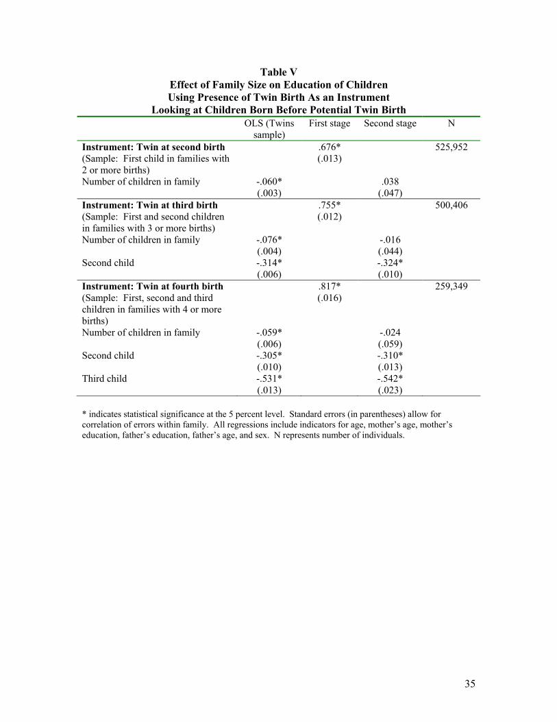
The 2SLS estimates are presented in Table V, along with the first stage
coefficients and the OLS estimates using the same sample. The first stage is very strong
and suggests that a twin birth increases completed family size by about 0.7 to 0.8. As
expected, twins at higher parity have a larger effect on family size, presumably because
they are more likely to push families above their optimal number of children. The t
statistics from the first stage are typically around 60, indicating that there are no concerns
about weak instruments in this application.

15
The 2SLS estimate of the effect on the first child of changes in family size
induced by the second birth being a twin birth is 0.038 (0.047). This implies no large
adverse effects of increased family size on educational outcomes (the lower bound of the
95 percent confidence interval is -.055). The equivalent estimate for families that have at
least 3 births is -0.016 (0.044), and for families that have at least 4 births it is -0.024
(0.059). The lower bound of the 95 percent confidence intervals for these estimates are -
.101, and -.140, respectively. Taken together, these three estimates are all less negative
than the OLS estimates and the first is precisely enough estimated to rule out large
negative effects of family size on education. These results are consistent with the
evidence in Table IV that family size has a negligible effect on children’s outcomes once
one controls for birth order.
3.7 Using same-sex as an instrument for family size
As described earlier, there is some question whether sex composition of siblings
has an independent effect on children’s outcomes. However, for completeness, we
describe results using this instrument here. We study the outcomes of the first two
children and use as the instrument whether or not these two children are the same sex.
The first stage is strong – a coefficient of 0.086 with a standard error of 0.002. The
second stage estimate is 0.28 (0.06), implying that increased family size leads to
significantly higher educational outcomes for children. We do not find the magnitude of
this estimate credible and suspect that there are independent positive effects on outcomes
of having a sibling of the same sex. Future research of our own will examine the direct
effects of family sex composition on children’s outcomes.

16
4. Birth Order
Given that birth order effects appear to drive the observed negative relationship
between family size and child education, we next turn our attention to birth order. Blake
[1989] describes some of the factors that make empirical estimation of birth order effects
difficult. First, it is necessary to fully control for family size or one will confound family
size and birth order effects. Second, the presence of cohort effects in educational
attainment will tend to bias results to the extent that later born children are in different
cohorts from earlier born children. Thus, one needs to have multiple cohorts for each
birth order and include unrestricted cohort effects. Third, it is important to include cohort
effects for the parents, as, conditional on child cohort, the parents of first-borns are likely
to be younger than parents of third or fourth born children.23
Studies of the effects of birth order on education have been limited by the absence
of the large representative datasets necessary to thoroughly address these issues. For
example, Behrman and Taubman [1986] use data on only about 1000 individuals from
the National Academy of Science/National Research Council twin sample and their adult
offspring. Hanushek [1992] uses a small sample of low-income black families collected
from the Gary Income Maintenance Experiment. Hauser and Sewell [1985] use the
Wisconsin Longitudinal Study; their data are less than ideal as, by definition, the survey
respondent has completed high school. Hauser and Sewell find no evidence for birth
order effects; Behrman and Taubman find some evidence that later children have lower
23 She also suggests that estimated birth order effects could be biased if spacing has an independent effect on outcomes and spacing differs on average by birth order. (Also see Powell and Steelman [1993].) To address this issue, we created 3 variables: (1) The number of children born within one year of the person, (2) the number of children born 2 or 3 years apart from the person, and (3) the number of children born 4 or 5 years apart from the person. Adding these variables to the regression had no appreciable effect on the estimated birth order effects. These specifications should be treated with some caution as spacing may be optimally chosen by families and, hence, is an endogenous variable.

17
education, and Hanushek observes a U-shaped pattern of achievement by birth order for
large families, with oldest and youngest children doing better than middle children
(although it is not clear that there are any statistically significant differences). However,
all these studies estimate birth order effects quite imprecisely and, due to small samples,
do not include the full set of family size indicators, cohort indicators, and parental cohort
indicators we use in this paper.
More recently, Iacovou [2001] uses the British National Child Development
Study (NCDS) and finds that later-born children have poorer educational outcomes than
earlier born. While this a very thorough study, it does suffer from some weaknesses. First
the sample size is small (about 18,000 initially) and there is much attrition over time
(about 50%) so estimates are imprecise and may be subject to attrition bias. Second, all
children in the sample are born the same week so, conditional on mother’s cohort, birth
order is strongly correlated with age at first birth and it is difficult to tease out separate
effects of these two variables.24
The empirical literature on the effect of birth order on children’s outcomes is
quite extensive; despite this, however, there have been no strong conclusions due to data
and methodological limitations.25 Because of our large dataset on the population of
Norway over an extended period of time, we are able to overcome most of the limitations
of the prior literature. Also, unlike the previous literature, we use family fixed effects
models in addition to OLS. Family fixed effects allow us to estimate effects of birth order
24 She does not control for age at first birth. Age at first birth is implicitly controlled for in our family fixed effects specifications. We have also added it as a control in our OLS models and doing so had little effect. 25 There is also an extensive literature in psychology and sociology on the effects of birth order on personality. See Conley [2004b] for a summary.

18
within families, thereby differencing out any family-specific characteristics that are
affecting all children.
4.1 Birth order results
The average education level and distribution of education by birth order are listed
in Table III; there is a clear pattern of declining education for higher birth orders.
However, as with the case of family size effects, these summary statistics can be
misleading in that we are not controlling for family size, cohort effects, or any other
demographic characteristics that may be influencing these statistics. As a result, we
estimate the relationship between birth order and educational attainment in a regression
framework, using the same set of control variables as in the family size analysis.
In Column 1 of Table VI, we present estimates for the full sample, including a full
set of family size dummies (presented in Table IV, Column 6). Relative to the first child,
we observe a steady decline in child’s education by birth order. The large magnitude of
the birth order effects relative to the family size effects is clear in Figure 1.
Each subsequent column in Table VI represents a separate regression for a
particular family size. If we look across row one, we can see the effect of being a
“second child” (omitted category is first child) is large and negative for all family sizes.
This is particularly striking, given that earlier work found somewhat different effects for
different family sizes [Hanushek 1992].26 As in Column 1, we find a monotonic decline
in average education as birth order increases. It is interesting to note that, in addition to
the monotonic decline in educational attainment by birth order, we also observe a
26 In his work, Hanushek also focuses on the effect of school quality by including such measures in the estimation; although we do not have school quality measures, we have tried adding municipality effects (schools are organized at the municipality level) and municipality-year effects to control for geographical

19
negative “last child” effect. This “last child” effect could be consistent with an optimal
stopping model in which parents continue to have children until they have a “poor
quality” child, at which point parents may opt to discontinue childbearing.27 However,
this model cannot explain the monotonic decline we observe in educational attainment of
the earlier children; for example, it cannot explain the large magnitudes of the second
child effect in families with more than two children.28
Table VII then presents the results with family fixed effects included. These
estimates are almost identical to those without family fixed effects, suggesting that the
estimated birth order effects do not reflect omitted family characteristics.29
5. Heterogeneous Effects of Family Size and Birth Order
In Table VIII we test the sensitivity of our results to various stratifications of our
sample. In Columns 1 and 2 of Table VIII, we first break the sample by sex. As one can
see, the results are quite similar for men and women; although statistically different from
zero, OLS family size effects (presented in the first row; these estimates include controls
for family background) become close to zero in magnitude when birth order is controlled
for (row 2). When we estimate the family size coefficients using the twin instrument, we
get small but imprecisely estimated coefficients for both men and women. (The third row
presents the coefficient on family size for the first child for the sample of families with at
least two children using twins at second birth as an instrument; the fourth row is the
and temporal differences in school quality; the inclusion of these variables does not affect our family size or birth order conclusions. 27 There is some evidence that early behaviors are reasonable predictors for later outcomes. (See Currie and Stabile[2004].) 28 This “last child" effect is also consistent with Zajonc's [1976] hypothesis that last children suffer from having nobody to teach. Also, last-born children may be more likely to have been “unwanted” children.

20
effect of family size on the first two children conditional on having at least three children
using twins at third birth as an instrument, and the fifth row is the effect of family size on
the first three children conditional on having at least four children using twins at fourth
birth as an instrument.) While, overall, the effects of family size for women seem smaller
than those for men, in both cases we see small family size effects. In contrast, birth order
effects are larger for women than for men.30
We also stratify our sample by mother’s educational attainment. (See Columns 3
and 4 in Table VIII.) This may be a relevant break if financial constraints are driving the
observed patterns; families with better educated mothers may be less financially
constrained than those with lower educated mothers. We find that the magnitude of the
birth order effects does not differ much across education groups; if anything, birth order
effects are stronger among individuals with more educated mothers, which runs counter
to the expected results if financial constraints were driving the results.
We next compare the effects of family size and birth order for earlier cohorts
relative to later cohorts. Later cohorts had the benefit of more effective birth control and,
as a result, parents may have exercised more control over completed family size. When
we stratify our sample based on mother’s cohort (those born before 1935 versus those
born after), we find similar effects of family size and birth order for both samples. (See
Table VIII, Columns 5 and 6.) While birth order effects are slightly smaller in the
younger sample relative to the older sample, they are still quite large and significant.
29 We have added controls for family size at ages 2 and 5, and this had little impact on the estimated birth order effects. This suggests that birth order is not just proxying for family size when young. 30 In these summary results (and in Table IX), we report birth order effects from family fixed effects specifications except in the case where we split the sample by sex. In this case, because we are missing family members in each sample, using fixed effects induces selection effects (for example, the only 2-child families used in the female sample are families with all girls), and provides rather imprecise estimates
21
It may be the case that birth order is proxying for family structure. Because we
don’t observe marital status of parents at each age, it may be that younger children are
more likely to be from broken homes and children from broken homes have lower
educational attainment. To test this, we examine the effect of family size and birth order
on educational attainment for a subset of children whose parents were still married in
1987 (the first year we have information on marital status); this includes approximately
60 percent of our sample.31 The results are presented in Column 7 of Table VIII. The
family size results are quite consistent with the results obtained using the full sample;
significant OLS coefficients, much smaller when we include birth order, and no
statistically significant effects using IV. While not reported in the table, it is interesting to
note that the negative only child effect observed in the full sample disappears when we
use the intact family subsample, suggesting that this result is in fact being driven by
family structure. Birth order effects are almost exactly the same as in the full sample,
implying that these effects do not result from marital breakdown.
6. Other Outcomes
Education is only one measure of human capital; we next examine the effect of
family size and birth order on labor market outcomes such as earnings and the probability
of working full time.32 In addition, teenage motherhood has been associated with many
(because so many families are omitted). When we do the male/female split, the birth order effects come from the OLS model with the full set of demographic controls and the full set of family size indicators. 31 Note that the youngest children in our sample would have been 12 at this time. We also tested the sensitivity of these results to looking only at children who were at least 30 in 2000; in this case, the youngest children would have been 17 at the point we are measuring family structure. The results are entirely insensitive to this age cutoff. 32 There is some previous research using labor market outcomes; for example, Kessler [1991] uses data from the NLSY to examine the effects of birth order and family size on wages and employment status. He finds that neither birth order nor childhood family size significantly influences the level or growth rate of

22
long-term economic and health disadvantages such as lower education, less work
experience and lower wages, welfare dependence, lower birth weights, higher rates of
infant mortality, and higher rates of participation in crime (Ellwood [1988]; Jencks
[1989]; Hoffman et al. [1993]). Therefore, we also study it as an outcome variable.
6.1 Labor market outcomes
We examine the effects of family size and birth order on the following labor
market outcomes: the earnings of all labor market participants, the earnings of full time
employees only, and the probability of being a full time employee. Descriptive statistics
for these variables are included in Table I. Earnings are measured as total pension-
qualifying earnings; they are not topcoded and include all labor income of the individual.
For the purposes of studying earnings and employment, we restrict attention to
individuals aged between 30 and 59 who are not full-time students. In this group,
approximately 90 percent of both men and women have positive earnings. Given this
high level of participation, our first outcome is log(earnings) conditional on having non-
zero earnings. Since the results for this variable encompass the effects on both wage rates
and hours worked, we also separately study the earnings of individuals who have a strong
attachment to the labor market and work full-time (defined as 30+ hours per week). 33 As
seen in Table I, about 71 percent of men and 46 percent of women are employed full time
in 2000. Our third outcome variable is whether or not the individual is employed full-
time (as defined above). We have chosen this as our employment outcome as most
wages. Also, Behrman and Taubman [1986] do not find evidence for birth order effects on earnings. Both of these papers suffer from very small sample sizes (generally fewer than 1000 observations). 33 To identify this group, we use the fact that our dataset identifies individuals who are employed and working full time at one particular point in the year (in the 2nd quarter in the years 86-95, and in the 4th quarter thereafter). An individual is labeled as employed if currently working with a firm, on temporary layoff, on up to two weeks of sickness absence, or on maternity leave.

23
individuals participate to some extent and, particularly for women, the major distinction
is between full-time and part-time work.
To maximize efficiency, we use all observations on individuals in the 1986-2000
panel, provided they are aged between 30 and 59. Because we have people from many
different cohorts, individuals are in the panel for different sets of years and at different
ages. Therefore, as before, we control for cohort effects. Also, we augment the previous
specification by adding indicator variables for the panel year. This takes account of
cyclical effects on earnings, etc. Some individuals are present in more periods than others
and, hence, have greater weight in estimation. We have verified that if we weight each
individual equally in estimation, we get similar but less precisely estimated coefficients.
None of our conclusions change. Also, the robust standard errors take account of the fact
that we have repeated observations on individuals.
Summary results for earnings are presented in Table IX. Because of the sizeable
differences in labor market experiences of men and women, we estimate separate
regressions by gender. The first three columns present the results for men and the second
three present the results for women. Interestingly, the earnings results are quite
consistent with the results obtained using education as the outcome. The OLS family size
effects become much smaller when birth order controls are introduced. Also, the family
size estimates using the twins instruments are always statistically insignificant, always
less negative than OLS, and generally have a positive sign. As with education, women
seem to be more affected by birth order; among women, the inclusion of the birth order
effects in the OLS regressions reduces the family size coefficient by more than half and
the birth order effects are quite large. While the effects are significant for men, they are

24
much smaller in magnitude. However, the differences between men and women are
much smaller when the sample is restricted to full-time employees. To get a sense of the
magnitude of these earnings effects, we estimated the return to education for the full-time
sample using the birth order indicators as instruments for education (including family size
indicators in addition to the usual controls); when we do this, we get an implied return of
approximately .05 for men and .07 for women, suggesting that much of the birth order
effects on earnings is likely working through education.34
We study the probability of working full time in Columns 3 and 6 of Table IX.
For computational reasons, we use linear probability models and do the IV estimation
using 2SLS.35 We find pronounced birth order effects for women (later-borns are less
likely to work full-time), and the addition of birth order effects reduces the OLS family
size estimate approximately in half. However, for men, the family size coefficient is
approximately the same with and without birth order effects, and the only significant
birth order effect is that fifth, sixth, and seventh children are more likely to work full time
than earlier born children.
6.2. Probability of having a teen birth
We present the effects of family size and birth order on the probability of having a
teen birth in Table IX, Column 7. We restrict the sample to women aged at least 36 in
2000 and denote a teen birth if they have a child that is aged at least 16 in 2000 who was
born before the woman was aged 20.36 The results are quite consistent with the earlier
34 Despite the significant birth order effects on earnings, they have a negligible effect on the within-family earnings variance. 35 The heteroskedasticity that results from the linear probability model is accounted for by our robust standard errors. 36 This sample restriction is required because to know whether a woman had a teen birth we need to observe both mother’s and child’s ages, so both must appear in the administrative data.

25
results for education; a positive OLS effect of family size on teenage pregnancy that
becomes significantly smaller when birth order effects are included. Once family size is
instrumented for with the twins indicator, the family size effect becomes statistically
insignificant. On the other hand, there are large birth order effects, with a move from
being the first child to the fourth child increasing the probability of having a child as a
teenager by almost five percentage points (the average probability of having a teen birth
is .13).
7. Conclusions
In this paper, we examine the effect of family size on child education using both
exogenous variation in family size induced by twin births as well as extensive controls
for not only parent and child cohort effects and parental education, but also birth order
effects. We find evidence that there is little if any family size effect on child education
once birth order is controlled for; this is true when we estimate the relationship with
controls for birth order or instrument family size with twin births.
Given that family sizes continue to decline in developed countries, these results
suggest that the children may not necessarily be better off than if their family had been
larger. Our results imply that, though average child outcomes may improve, there may be
little effect on first-born children.
In contrast, we find very large and robust effects of birth order on child education.
To get a sense of the magnitude of these effects, the difference in educational attainment
between the first child and the fifth child in a five child family is roughly equal to the
difference between black and white educational attainment calculated from the 2000
census. We augment the education results by using earnings, whether full-time employed,

26
and whether had a birth as a teenager as additional outcome variables. We also find
strong evidence for birth order effects with these other outcomes, particularly for women.
Later-born women have lower earnings (whether employed full-time or not), are less
likely to work full-time, and are more likely to have their first birth as a teenager. In
contrast, while later-born men have lower full-time earnings, they are not less likely to
work full-time.
These sizeable birth order effects have potential methodological implications:
Researchers using sibling fixed effects models to study economic outcomes may obtain
biased estimates unless they take account of birth order effects in their estimation.
One important issue remains unresolved: what is causing the birth order effects
we observe in the data? Our findings are consistent with optimal stopping being a small
part of the explanation. Also, the large birth order effects found for highly educated
mothers, allied with the weak evidence for family size effects, suggest that financial
constraints may not be that important. Although a number of other theories (including
time constraints, endowment effects, and parental preferences) have been proposed in the
literature, we are quite limited in our ability to distinguish between these models. Finding
relevant explanations will have important implications for models of household allocation
(which can predict both compensatory or reinforcing behavior on the part of parents and
also depend on differences in endowments and preferences) and models of child
development.
Our findings so far are quite provocative; if, in fact, there is no independent
tradeoff between family size and child quality, perhaps we need to revisit models of
fertility and reconsider what should be included in the “production function” of children.

27
What other explanations will generate the patterns we observe in the data? Clearly, our
results suggest a need for more work in this area.
Sandra E. Black
Department of Economics
UCLA, IZA and NBER
Paul J. Devereux
Department of Economics
UCLA and IZA
Kjell G. Salvanes
Department of Economics
Norwegian School of Economics, Statistics Norway and IZA

28
References
Aakvik, Arild, Kjell G. Salvanes, and Kjell Vaage, “Measuring the Heterogeneity in the Returns to Education in Norway Using Educational Reforms,” CEPR DP 4088, Revised October 2004.
Angrist, Joshua D., and William N. Evans, “Children and Their Parents’ Labor Supply:
Evidence from Exogenous Variation in Family Size,” American Economic Review, LXXXVIII (1998), 450-477.
Becker, Gary S., “An Economic Analysis of Fertility,” Demographic and Economic
Change in Developed Countries, Gary S. Becker, ed. (Princeton, NJ: Princeton University Press, 1960).
Becker, Gary S., and Robert J. Barro, “A Reformulation of the Economic Theory of
Fertility,” Quarterly Journal of Economics, CIII (1988), 1-25. Becker, Gary S., and H. Gregg Lewis, “On the Interaction Between the Quantity and
Quality of Children,” Journal of Political Economy, LXXXI (1973), S279-S288. Becker, Gary S., and Nigel Tomes, “Child Endowments and the Quantity and Quality of
Children,” Journal of Political Economy, LXXXIV (1976), S143-S162. Behrman, Jere R., and Paul Taubman, “Birth Order, Schooling, and Earnings,” Journal
of Labor Economics, IV (1986), S121-145. Blake, Judith, Family Size and Achievement, (Berkeley and Los Angeles, CA: University
of California Press, 1989). Bronars, Stephen G., and Jeff Grogger, “The Economic Consequences of Unwed
Motherhood: Using Twin Births as a Natural Experiment,” American Economic Review, LXXXIV (1994), 1141-1156.
Butcher, Kristin F., and Anne Case, "The Effect of Sibling Sex Composition on Women's
Education and Earnings," Quarterly Journal of Economics, CIX (1994), 531-563. Conley, Dalton, “What is the “true” effect of sibship size and birth order on education?
Instrumental variable estimates from exogenous variation in fertility,” Mimeo, 2004.
Conley, Dalton, "Sibling Sex Composition: Effects on Educational Attainment," Social
Science Research, XXIX (2000), 441-457. Conley, Dalton, The Pecking Order: Which Siblings Succeed and Why, (New York, NY:
Pantheon Books, 2004b).

29
Currie, Janet, and Mark Stabile, “Child Mental Health and Human Capital Accumulation: The Case of ADHD,” Working paper, 2004.
Dahl, Gordon, and Enrico Moretti, “The Demand for Sons: Evidence from Divorce,
Fertility, and Shotgun Marriage,” National Bureau of Economic Research Working paper No. 10281, 2004.
Deschenes, Olivier, "Estimating the Effects of Family Background on the Return to
Schooling," University of California Santa Barbara Departmental Working Paper No. 10-02, 2002.
Doepke, Matthias, “Accounting for Fertility Decline During the Transition to Growth,”
Working Paper, 2003. Ellwood, David, Poor Support, (New York, NY: Basic Books, 1988). Goux, Dominique, and Eric Maurin, “The Effect of Overcrowded Housing on Children’s
Performance at School,” Mimeo, 2004. Guo, Guang, and Leah K. VanWey, “Sibship Size and Intellectual Development: Is the
Relationship Causal?,” American Sociological Review, LXIV (1999), 169-187. Hanushek, Eric A., “The Trade-off between Child Quantity and Quality,” Journal of
Political Economy, C (1992). 84-117. Hauser, Robert M., and Hsiang-Hui Daphne Kuo, "Does the Gender Composition of
Sibships affect Women's Educational Attainment?," Journal of Human Resources, XXXIII (1998), 644-657
Hauser, Robert M., and William H. Sewell, "Birth Order and Educational Attainment in
Full Sibships," American Educational Research Journal, XXII (1985), 1-23. Hoffman S.D., Foster, E.M., and F.F. Furstenberg jr., “Reevaluating the Costs of Teenage
Childbearing,” Demography, XXX (1993), 1-13. Iacovou, Maria, "Family Composition and Children's Educational Outcomes," Working
Paper, 2001. Jacobsen, Joyce P., James Wishart Pearce III, and Joshua L. Rosenbloom, “The Effects of
Childbearing on Married Women’s Labor Supply and Earnings: Using Twin Births as a Natural Experiment,” Journal of Human Resources, XXXIV (1999), 449-474.
Jencks, Christopher, “What is the Underclass – and is it Growing?,” Focus, XII (1989),
14-26.

30
Kaestner, Robert, “Are Brothers Really Better? Sibling Sex Composition and Educational Attainment Revisited,” Journal of Human Resources, XXXII (1997), 250-284. Kessler, Daniel, “Birth Order, Family Size, and Achievement: Family Structure and
Wage Determination,” Journal of Labor Economics, IX (1991), 413-426. Lee, Jungmin, "Children and Household Education Decisions: An Asian Instrument,"
Working Paper, 2003. Møen, Jarle, Kjell G. Salvanes, and Erik Sørensen, ”Documentation of the Linked
Employer-Employee Data Base at the Norwegian School of Economics and Business Administration,” Mimio, Norwegian School of Economics, 2004.
Noack, Turid and Lars Ostby. 1981. Fruktbarhet blant norske kvinner. Resultater fra
fruktbarhetsundersøkelsen 1977. (fertility among Norwegian women. Results from the fertility survey 1977. Statistics Norway. Samfunnsøkonomiske studier no. 49.
Phillips, Meredith, “Sibship Size and Academic Achievement: What We Now Know and
What We Still Need to Know—Comment on Guo & VanWey,” American Sociological Review, LXIV (1999), 188-192.
Powell, Brian, and Lala Carr Steelman, “The Educational Benefits of Being Spaced Out:
Sibship Density and Educational Progress,” American Sociological Review, LVIII (1993), 367-381.
Rosenzweig Mark R., and Kenneth I. Wolpin, "Testing the Quantity-Quality Fertility
Model: The Use of Twins as a Natural Experiment,” Econometrica, XLVIII (1980), 227-240.
Rosenzweig Mark R., and Kenneth I. Wolpin, "Natural "Natural Experiments" in
Economics,” Journal of Economic Literature, XXXVII (2000), 827-874. Skrede, Kari, "Drmmer, dyder, og belonning" ("Dreams and rewards") Report from
Statistics Norway No 106, (1999). Zajonc R. B., “Family Configuration and Intelligence,” Science, CXCII (1976), 227-236.

31
Table I Summary Statistics-Full Sample
Mean Standard deviation Age in 2000 38 8.5 Female .48 .50 Education 12.2 2.4 Mother’s Education 9.5 2.4 Father’s Education 10.4 3.0 Mother’s Age in 2000 65 10.5 Father’s Age in 2000 67 10.0 Number of Children 2.96 1.3 Twins in Family .015 .12 Men: Log Earnings in 2000 12.55 .77 Log FT Earnings in 2000 12.72 .45 Proportion FT in 2000 .71 .45 Women: Log Earnings in 2000 12.05 .88 Log FT Earnings in 2000 12.42 .42 Proportion FT in 2000 .46 .50 Prob (Teen Birth) .13 .34 Descriptive statistics are for 1,427,100 children from 647,035 families. All children are aged at least 25 in 2000. Twins are excluded from the sample. All children and parents are aged between 16 and 74 at some point between 1986 and 2000. Earnings are in Norwegian Kroner and FT indicates working 30+ hours per week. Source: Matched Administrative Data from Statistics Norway
Table II Number of Children in the Family (by Family)
Frequency Percentage 1 116,000 17.9 2 264,627 40.9 3 171,943 26.9 4 63,810 9.9 5 20308 3.1 6 6674 1.0 7 2251 .4 8 822 .1 9 350 .05 10+ 250 .04 All children are aged at least 25 in 2000. Twins are excluded from the sample. All children and parents are aged between 16 and 74 at some point between 1986 and 2000. Source: Matched Administrative Data from Statistics Norway

32
Table III Average Education by Number of Children in Family and Birth Order
Average education
Average mother’s education
Average father’s
education
Fraction with <12
years
Fraction with 12 years
Fraction with >12
years Family size
1 12.0 9.2 10.1 .44 .25 .31 2 12.4 9.9 10.8 .34 .31 .35 3 12.3 9.7 10.6 .37 .30 .33 4 12.0 9.3 10.1 .43 .29 .28 5 11.7 8.8 9.5 .49 .27 .24 6 11.4 8.5 9.1 .54 .25 .20 7 11.2 8.3 8.9 .57 .24 .19 8 11.1 8.2 8.8 .58 .24 .18 9 11.0 8.0 8.6 .59 .25 .16 10+ 11.0 7.9 8.8 .59 .26 .15
Birth order 1 12.2 9.7 10.6 .38 .28 .34 2 12.2 9.6 10.5 .38 .30 .31 3 12.0 9.3 10.2 .40 .31 .29 4 11.9 9.0 9.7 .43 .32 .25 5 11.7 8.6 9.2 .46 .31 .22 6 11.6 8.3 8.9 .49 .31 .20 7 11.5 8.1 8.7 .51 .30 .19 8 11.6 8.0 8.6 .49 .31 .20 9 11.3 7.9 8.4 .53 .32 .15 10+ 11.3 7.8 8.7 .52 .32 .15 All 12.2 9.5 10.4 .39 .29 .32
Descriptive statistics are for 1,427,100 children from 647,035 families. All children are aged at least 25 in 2000. Twins are excluded from the sample. All children and parents are aged between 16 and 74 at some point between 1986 and 2000. Source: Matched Administrative Data from Statistics Norway

33
Table IV Effect of Family Size on Children’s Education Dependent variable: Child’s education
No demographic controls
With demographic controls
Demographic and birth order controls
Number of children -.182*
(.002) -.095*
(.002) -.013*
(.002)
2 child family .272* (.009)
.096* (.008)
.257* (.008)
3 child family .132* (.009)
.001* (.008)
.270* (.009)
4 child family -.176* (.010)
-.149* (.009)
.195* (.010)
5 child family -.481* (.014)
-.279* (.012)
.115* (.013)
6 child family -.730* (.021)
-.394* (.018)
.034 (.019)
7 child family -.882* (.034)
-.472* (.029)
-.018 (.031)
8 child family -.947* (.053)
-.502* (.045)
-.039 (.046)
9 child family -1.036* (.072)
-.522* (.065)
-.037 (.067)
10 child family -1.198* (.084)
-.614* (.075)
-.090 (.079)
Second child -.294* (.004)
-.342* (.004)
Third child -.494* (.007)
-.538* (.007)
Fourth child -.632* (.010)
-.621* (.010)
Fifth child -.718* (.015)
-.648* (.015)
Sixth child -.782* (.023)
-.661* (.023)
Seventh child -.854* (.037)
-.709* (.037)
Eighth child -.753* (.059)
-.605* (.057)
Ninth child -.945* (.081)
-.800* (.082)
Tenth child -1.131* (.116)
-.981* (.111)
N 1,427,100 1,427,100 1,427,100 1,427,100 1,427,100 1,427,100R2 .0465 .0498 .1949 .1954 .1989 .1999
* indicates statistical significance at the 5 percent level. Standard errors (in parentheses) allow for correlation of errors within family. All regressions include indicators for age, mother’s age, and sex.

34
Demographic controls include indicators for mother’s education, father’s education, and father’s age. N represents number of individuals.
35
Table V Effect of Family Size on Education of Children Using Presence of Twin Birth As an Instrument
Looking at Children Born Before Potential Twin Birth OLS (Twins
sample) First stage Second stage N
Instrument: Twin at second birth (Sample: First child in families with 2 or more births)
.676* (.013)
525,952
Number of children in family -.060* (.003)
.038 (.047)
Instrument: Twin at third birth (Sample: First and second children in families with 3 or more births)
.755* (.012)
500,406
Number of children in family -.076* (.004)
-.016 (.044)
Second child -.314* (.006)
-.324* (.010)
Instrument: Twin at fourth birth (Sample: First, second and third children in families with 4 or more births)
.817* (.016)
259,349
Number of children in family -.059* (.006)
-.024 (.059)
Second child -.305* (.010)
-.310* (.013)
Third child -.531* (.013)
-.542* (.023)
* indicates statistical significance at the 5 percent level. Standard errors (in parentheses) allow for correlation of errors within family. All regressions include indicators for age, mother’s age, mother’s education, father’s education, father’s age, and sex. N represents number of individuals.

Table VI Effect of Birth Order on Children’s Education
Estimated by Family Size All families1 Two
child family
Three child
family
Four child
family
Five child
family
Six child
family
Seven child
family
Eight child
family
Nine child
family
Ten child
family Second child -.342*
(.004) -.378* (.007)
-.318* (.007)
-.327* (.012)
-.278* (.020)
-.256* (.035)
-.247* (.063)
-.449* (.104)
-.284* (.172)
-.350* (.174)
Third child -.538* (.007)
-.610* (.011)
-.558* (.015)
-.488* (.024)
-.493* (.040)
-.460* (.072)
-.632* (.115)
-.595* (.189)
-.626* (.208)
Fourth child -.621* (.010)
-.768* (.021)
-.646* (.030)
-.659* (.047)
-.610* (.081)
-.695* (.134)
-.480* (.199)
-.877* (.226)
Fifth child -.648* (.015)
-.815* (.040)
-.701* (.059)
-.704* (.097)
-.841* (.150)
-.662* (.222)
-.936* (.245)
Sixth child -.661* (.023)
-.872* (.073)
-.742* (.117)
-.813* (.171)
-.638* (.257)
-1.042* (.262)
Seventh child -.709* (.037)
-.873* (.141)
-1.024* (.203)
-.696* (.271)
-1.241* (.287)
Eighth child -.605* (.057)
-1.013* (.236)
-.460 (.319)
-1.445* (.314)
Ninth child -.800* (.082)
-.816* (.373)
-1.569* (.343)
Tenth child -.981* (.111)
-1.919* (.399)
N 1,427,100 478,957 449,799 227,697 92,203 36,645 14,412 6,074 2,878 2,435
* indicates statistical significance at the 5 percent level. Standard errors (in parentheses) allow for correlation of errors within family. Each column represents a separate regression. All regressions include indicators for age, mother’s age, mother’s education, father’s education, father’s age, and sex. 1 In this specification, indicator variables for family size are also included in the regression. N represents number of individuals.

37
Table VII Effect of Birth Order on Children’s Education
Estimated by Family Size Family Fixed Effects
All families1
Two child
family
Three child
family
Four child
family
Five child
family
Six child
family
Seven child
family
Eight child
family
Nine child
family
Ten child
family Second child -.340*
(.005) -.415* (.011)
-.315* (.009)
-.313* (.012)
-.264* (.021)
-.231* (.034)
-.216* (.059)
-.472* (.096)
-.280 (.151)
-.366* (.170)
Third child -.531* (.009)
-.598* (.017)
-.524* (.018)
-.458* (.027)
-.451* (.042)
-.410* (.070)
-.681* (.111)
-.593* (.172)
-.666* (.188)
Fourth child -.612* (.014)
-.708* (.028)
-.592* (.037)
-.593* (.054)
-.532* (.086)
-.778* (.135)
-.498* (.203)
-.918* (.214)
Fifth child -.641* (.020)
-.734* (.051)
-.611* (.069)
-.575* (.107)
-.950* (.164)
-.696* (.242)
-.967* (.246)
Sixth child -.659* (.028)
-.749* (.090)
-.604* (.132)
-.939* (.197)
-.686* (.286)
-1.081* (.284)
Seventh child -.706* (.042)
-.674* (.164)
-1.160* (.237)
-.791* (.339)
-1.293* (.328)
Eighth child -.607* (.062)
-1.153* (.286)
-.612 (.396)
-1.532* (.368)
Ninth child -.808* (.094)
-.998* (.472)
-1.647* (.416)
Tenth child -.940* (.118)
-1.982* (.483)
N 1,427,100 478,957 449,799 227,697 92,203 36,645 14,412 6,074 2,878 2,435 * indicates statistical significance at the 5 percent level. Standard errors are in parentheses. Each column represents a separate regression. All regressions include indicators for age and sex. N represents number of individuals.

Table VIII Family Size and Birth Order Effects
By Gender, Mother’s Education, Cohort, and Family Structure Males Females Mother’s
education ≤12
Mother’s education
>12
Mother born
before 1935
Mother born after 1935
Intact families
Family size OLS -.093*
(.002) -.095* (.002)
-.099* (.002)
-.021* (.007)
-.083* (.003)
-.120* (.003)
-.116* (.003)
OLS with birth order
-.025* (.003)
.002 (.003)
-.015* (.002)
.071* (.008)
-.016* (.003)
-.011* (.003)
-.032* (.003)
IV – twin at 2nd birth
.031 (.066)
.054 (.078)
.044 (.052)
-.089 (.122)
.100 (.077)
-.007 (.058)
.016 (.062)
IV – twin at 3rd birth
-.031 (.060)
-.001 (.057)
-.042 (.047)
.098 (.121)
.018 (.069)
-.051 (.054)
-.066 (.055)
IV – twin at 4th birth
-.079 (.077)
-.036 (.078)
-.012 (.062)
-.169 (.203)
-.065 (.085)
.022 (.077)
.001 (.074)
Birth order Second child -.301*
(.006) -.382* (.006)
-.329* (.006)
-.293* (.019)
-.389* (.008)
-.305* (.007)
-.311* (.007)
Third child -.462* (.009)
-.615* (.010)
-.504* (.010)
-.523* (.036)
-.601* (.014)
-.476* (.014)
-.500* (.012)
Fourth child -.513* (.014)
-.732* (.014)
-.583* (.014)
-.626* (.056)
-.691* (.020)
-.549* (.021)
-.587* (.018)
Fifth child -.538* (.022)
-.766* (.022)
-.620* (.020)
-.667* (.088)
-.725* (.026)
-.579* (.031)
-.625* (.026)
Sixth child -.527* (.034)
-.803* (.035)
-.646* (.028)
-.679* (.149)
-.745* (.036)
-.603* (.049)
-.657* (.036)
Seventh child -.528* (.052)
-.907* (.057)
-.687* (.042)
-.874* (.264)
-.818* (.051)
-.588* (.084)
-.728* (.054)
Eighth child -.380* (.087)
-.871* (.085)
-.599* (.063)
-1.046* (.395)
-.711* (.074)
-.536* (.135)
-.664* (.078)
Ninth child -.669* (.109)
-.945* (.131)
-.825* (.096)
-1.136 (.702)
-.921* (.110)
-.715* (.226)
-.812* (.120)
Tenth child -.912* (.151)
-1.058* (.169)
-.914* (.119)
-2.378* (.934)
-1.099* (.136)
-.426 (.313)
-1.239* (.142)
* indicates statistical significance at the 5 percent level. All family size regressions include indicators for age, sex, mother’s age, mother’s education, father’s education, and father’s age. The third row presents the coefficient on family size for the first child for the sample of families with at least two children, using twins at second birth as an instrument; the fourth row is the effect of family size on the first two children conditional on having at least three children using twins at third birth as an instrument, and the fifth row is the effect of family size on the first three children conditional on having at least four children using twins at fourth birth as an instrument. The IV estimates include a full set of birth order controls. The Birth order estimates come from family fixed effects specifications that include age indicators plus a sex indicator except for Columns 1 and 2, where birth order effects are from specifications that include the controls listed above plus a full set of family size indicators. N represents number of individuals. Sample sizes are:

39
744,292 for Column 1, 682,808 for Column 2, 1,251,988 for Column 3, 162,291 for Column 4, 709,700 for Column 5, 717,400 for Column 6, and 772,985 for Column 7.

40
Table IX
Family Size and Birth Order Effects Men Women Log
(earnings) Log
(earnings) given full
time
Prob
work full time
Log (earnings)
Log (earnings) given full
time
Prob
work full time
Prob of teen birth
Family size OLS -.015*
(.001) -.010* (.0004)
-.040* (.0004)
-.020* (.001)
-.011* (.0005)
-.010* (.0004)
.016* (.0005)
OLS with birth order
-.012* (.001)
-.006* (.0005)
-.011* (.0005)
-.010* (.001)
-.010* (.001)
-.006* (.001)
.010* (.001)
IV – twin at 2nd birth
-.003 (.020)
-.005 (.014)
-.005 (.013)
.030 (.026)
.015 (.016)
.021 (.015)
-.018 (.013)
IV – twin at 3rd birth
.013 (.018)
.019 (.012)
-.010 (.012)
.013 (.022)
.005 (.014)
.013 (.012)
-.005 (.011)
IV – twin at 4th birth
.022 (.020)
.002 (.014)
-.003 (.013)
.013 (.026)
-.006 (.016)
.024 (.015)
.026 (.015)
Birth order Second child -.012*
(.002) -.018* (.001)
.0016 (.0013)
-.042* (.003)
-.027* (.002)
-.021* (.001)
.022* (.001)
Third child -.028* (.003)
-.031* (.002)
-.001 (.002)
-.066* (.004)
-.040* (.002)
-.031* (.002)
.040* (.002)
Fourth child -.031* (.004)
-.038* (.003)
.001 (.003)
-.088* (.006)
-.052* (.004)
-.035* (.003)
.050* (.003)
Fifth child -.030* (.007)
-.040* (.004)
.010* (.005)
-.091* (.009)
-.057* (.006)
-.038* (.005)
.056* (.006)
Sixth child -.025* (.012)
-.038* (.007)
.018* (.008)
-.077* (.015)
-.048* (.009)
-.038* (.008)
.054* (.009)
Seventh child -.013 (.020)
-.036* (.012)
.028* (.012)
-.111* (.025)
-.091* (.018)
-.056* (.013)
.084* (.017)
Eighth child -.033 (.034)
-.051* (.019)
-.008 (.020)
-.114* (.041)
-.109* (.031)
-.041* (.019)
.064* (.025)
Ninth child -.011 (.047)
-.025 (.022)
.039 (.029)
-.144* (.074)
-.080 (.049)
-.105* (.029)
.066 (.042)
Tenth child -.017 (.053)
-.085 (.043)
.044 (.039)
-.212 (.087)
-.208* (.056)
-.035 (.041)
.050 (.054)
* indicates statistical significance at the 5 percent level. All family size regressions include indicators for age, sex, mother’s age, mother’s education, father’s education, and father’s age. The third row presents the coefficient on family size for the first child for the sample of families with at least two children, using twins at second birth as an instrument; the fourth row is the effect of family size on the first two children conditional on having at least three children using twins at third birth as an instrument, and the fifth row is the effect of family size on the first three children conditional on having at least four children using twins at fourth birth as an instrument. The IV estimates include a full set of birth order controls. The Birth Order estimates come from specifications that include the controls listed above plus a full set of family size indicators. The sample sizes differ between columns. In column 1 there are 5,503,423 observations on 590,879 men; in column 2 there are 4,125,280 observations on 525,225 men, in column 3 there are

41
5,900,902 observations on 604,703 men, in column 4 there are 4,532,190 observations on 528,137 women, in column 5 there are 2,080,870 observations on 368,887 women, in column 6 there are 5,154,202 observations on 547,819 women, and in column 7 there are 378,534 women with one observation per person.

42
Effect of Family Size and Birth Order on Educational Attainment
Relative to the Educational Attainment of a Child in a Single Child Family
-1.2
-1
-0.8
-0.6
-0.4
-0.2
0
0.2
0.4
1 2 3 4 5 6 7 8 9 10
Birth Order
2 Child Family 3 Child Family 4 Child Family 5 Child Family 6 Child Family 7 Child Family8 Child Family 9 Child Family 10 Child Family
Figure I

CENTRE FOR THE ECONOMICS OF EDUCATION Recent Discussion Papers
49 S. McNally E. Maurin
Vive la Révolution! Long Term Returns of 1968 to the angry students
48 L. Dearden L. McGranahan B. Sianesi
The Role of Credit Constraints in Educational Choices: Evidence from the NCDS and BCS70
47 R. Blundell L. Dearden B. Sianesi
Evaluating the Impact of Education on Earnings in the UK: Models, Methods and Results from NCDS
46 L. Dearden L. McGranahan B. Sianesi
An In-Depth Analysis of the Returns to National Vocational Qualifications Obtained at Level 2
45 L. Dearden L. McGranahan B. Sianesi
Returns to Education for the ‘Marginal Learner’: Evidence from the BCS70
44 F. Galindo-Rueda O. Marcenaro-Gutierrez A. Vignoles
The Widening Socio-Economic Gap in UK Higher Education
43 S. Machin S. McNally
The Literacy Hour
42 S. Gibbons S. Machin
Paying for Primary Schools: Supply Constraints, School Popularity or Congestion?
41 J. Blanden P.Gregg
Family Income and Educational Attainment: A Review of Approaches and Evidence for Britain
40 A. Chevalier Parental Education and Child’s Education: A Natural Experiment
39 A. Jenkins Women, Lifelong Learning and Employment
38 A. Jenkins R. Levacic
Evaluating the Effectiveness of Specialist Schools

37 A. Jenkins A. Wolf
Regional Variations in Adult Learning and Vocational Training: Evidence from NCDS and WERS 98
36 L. Feinstein F. Galindo-Rueda A. Vignoles
The Labour Market Impact of Adult Education and Training: A Cohort Analysis
35 S. McIntosh Further Analysis of the Returns to Academic and Vocational Qualifications
34 J.S. Pischke The Impact of the School Year on Student Performance and Earnings: Evidence from the German Short School Year
33 A. Chevalier G. Conlon
Does it Pay to Attend a Prestigious University?
32 F. Galindo-Rueda A. Vignoles
Class Ridden or Meritocratic? An Economic Analysis of Recent Changes in Britain
31 F. Galindo-Rueda Employer Learning and Schooling-Related Statistical Discrimination in Britain
30 R. Dur C. Teulings
Are Education Subsides an Efficient Redistributive Device?
A. Chevalier G. Conlon F. Galindo-Rueda S. McNally
Research Report to the Department for Education & Skills: The Returns to Higher Education Teaching
To order a discussion paper, please contact the Publications Unit
Centre for Economic Performance Tel 020 7955 7673 Fax 020 7955 7595