The Micro and Macro of Managerial Beliefs

Jose Maria Barrero∗

[Job Market Paper]

Updated frequently. For latest version please go to:web.stanford.edu/∼barreroj/BarreroJMP.pdf

Appendix here

December 18, 2018

Abstract

I study how biases in managerial beliefs affect firm performance and the macro-economy.Using confidential survey data to test whether US managers have biased beliefs, I establishthree facts. (1) Managers are neither over-optimistic nor pessimistic: their forecasts for futuresales growth are correct on average. (2) Managers are overconfident: they underestimate futuresales growth volatility. (3) Managers overextrapolate: their forecasts are too optimistic orpessimistic depending on whether the firm is growing or shrinking at the time of the forecast.To quantify the micro and macro implications of these facts, I build and estimate a generalequilibrium model in which managers of heterogeneous firms may have biased beliefs and makedynamic hiring decisions subject to adjustment costs. Biased managers in the model overreactto changes in their firm’s profitability because they believe profitability is more persistent andstable than it really is. The model thus implies that a typical firm’s value would increase by1.9 percent if it hired a rational manager. At the macro level, pervasive overreaction results intoo many resources spent on reallocation. Welfare would be higher by 1 percent in an economywith rational managers.

∗Stanford University, barreroj@stanford.edu, http://web.stanford.edu/~barrerojI thank Nick Bloom, Monika Piazzesi, Pete Klenow, Amit Seru, and Juliane Begenau for their invaluable guidanceand advice. I also thank Adrien Auclert, Katy Bergstrom, Steve Davis, William Dodds, Paul Dolfen, Ricardo dela O, Bob Hall, Charles Hodgson, Eran Hoffmann, Pablo Kurlat, Sean Myers, Bobby Pakzad-Hurson, AlessandraPeter, Nicola Pierri, Martin Schneider, Stephen Terry, Chris Tonetti, and various seminar participants at Stanford forhelpful comments. I benefitted immensely from attending the 2017 Mitsui Summer School on Structural Estimationin Corporate Finance. I’m also grateful with David Altig, Michael Bryan, Brent Meyer, and Nicholas Parker at theFederal Reserve Bank of Atlanta for access and assistance with the data from the Survey of Business Uncertainty.Financial support from the Ewing Marion Kauffman Foundation via the Kauffman Dissertation Fellowship and fromthe B.F. Haley and E.S. Shaw Fellowship for Economics through a grant to the Stanford Institute for Economic PolicyResearch are gratefully acknowledged. All errors are my own.This research was partially funded by the Ewing Marion Kauffman Foundation. The contents of this paper are solelythe responsibility of Jose Maria Barrero.

1

1 Introduction

Optimal management of a firm subject to uncertainty generally requires its manager to have correctbeliefs about the firm’s future business conditions. Intuitively, a manager who has biased beliefs maymake mistakes that destroy some of the firm’s value. If biases are a pervasive feature of managerialbeliefs, the sum of individual managers’ mistakes may additionally affect the macroeconomy. Whileit is easy to make this string of arguments, the question is ultimately an empirical and quantitativeone: how –and by how much– do biases in managerial beliefs matter?

This paper develops new empirical measures of the extent to which US managers have biasedbeliefs and provides some of the first estimates of how biases impact the value of individual firmsand the macro-economy. I use data from a confidential survey of US managers to test whether theyhave biased beliefs about their own firm’s future sales growth. Based on these empirical findings,I build and estimate a general equilibrium model in which biased managers make dynamic hiringdecisions subject to uncertainty and adjustment costs. Using my estimated model I infer how coun-terfactual, rational managers would behave under the same environment and thus quantify how firmperformance and macroeconomic outcomes would differ if managers were rational. My counterfac-tual experiments show biased managers overreact to changes in their firm’s business conditions andoverspend on adjustment costs, leading them to destroy 1.9 percent of the typical firm’s value andcollectively reduce aggregate welfare by about 1 percent of aggregate consumption.

I test for biases in US managers’ beliefs using the Atlanta Fed/Chicago-Booth/Stanford Surveyof Business Uncertainty (SBU), which is fielded by the Federal Reserve Bank of Atlanta (see Altiget al. (2018) for details). The SBU has been in the field monthly since October 2014, collecting dataon manager beliefs about future outcomes at their own firm, in particular sales growth over the fourquarters following the survey. Respondents are high-level managers like CFOs and CEOs, or othersinvolved in decision-making. SBU responses are confidential and collected by a Federal ReserveBank, so there are no obvious motives for respondents to misreport their beliefs in the survey.Furthermore, the SBU is especially well-suited to measuring the extent of biases in managerialbeliefs because it asks respondents for five possible sales growth scenarios looking over the next fourquarters (i.e. a lowest, low, middle, high, and highest scenario), and then asks them to assign aprobability to each scenario. Since I observe these five-point approximations of managers’ subjectivedistributions, I measure both their subjective expectations (i.e. their forecasts) and their subjectiveuncertainty about future sales growth and assess whether both their first and second moments areconsistent with ex-post realizations.

How biased do managers appear in the SBU data? I answer this question by documenting threefacts. First, managers appear neither systematically optimistic nor pessimistic: pooling across firmsand survey dates, I estimate the average forecast minus realized sales growth to be indistinguishablefrom zero.1 Second, managers responding to the SBU are overconfident ; that is, they underestimatethe volatility of future sales growth and overestimate their forecasts’ accuracy. While managers’

1See Bachmann and Elstner (2015) for a similar finding among German manufacturing firms.

2

subjective distributions would imply an average absolute forecast error of about 4 percentage points,in reality the mean absolute forecast error is close to 18 percentage points, more than four timesas large. This discrepancy points to a significant deviation from rational expectations. Third,managers overextrapolate from current conditions. If the manager’s firm experiences high salesgrowth in a quarter when she responds to the SBU, her forecast tends to overestimate the firm’sactual performance over the subsequent four quarters. If, instead, the firm experiences shrinkingsales, the manager tends to underestimate. This pattern is consistent with managers overstatingthe degree to which the current state of affairs – positive or negative – will continue to persist intothe future, a common finding in the forecasting and psychology literatures.2 Quantitatively, foreach additional percentage point of sales growth during the quarter of the forecast the manageroverestimates future performance by an additional 0.2 percentage points. Again, this is a significantdeparture from rational expectations.

To understand how biases impact individual firms and the macro-economy, I build a generalequilibrium model with heterogeneous firms run by managers who may have biased beliefs. Managersin the model may misperceive the overall mean, persistence, and volatility of business conditions,with each of these three potential biases corresponding to one of the three facts I document inthe SBU data. Managers in the model choose the firm’s labor under uncertainty, forecasting futureconditions under their own, possibly biased beliefs. These hiring decisions are subject to adjustmentcosts that force managers to trade off the perceived benefit of hiring or laying off workers againstthe cost of making those adjustments. Theoretically, the presence of adjustment costs means thathiring or laying off workers involves up-front costs that managers may later regret having paid,increasing the stakes in managerial decisions. Empirically, adjustment costs also help the modelaccount for the joint dynamics of firm-level sales and employment, which are positively but notperfectly correlated in the data.

I quantify the implications of managerial mistakes by confronting the model against the SBUdata, structurally estimating the parameters that empirically account for: (1) the extent of man-agerial optimism, overconfidence, and overextrapolation; and, (2) the joint behavior of sales andemployment, the two key endogenous variables in my model that I also observe in the SBU. In-tuitively, the statistics I use to test for managerial biases are informative of the extent of biases,conditional on the technology and environment in which their firms operate. Employment and salesgrowth fluctuations, in turn, are informative of the technology, uncertainty, and frictions managersface as they make forward-looking decisions given some beliefs. By matching moments relatedboth to managerial biases and decisions I discipline the structural parameters that are crucial forinferring how managers would behave if they had different beliefs. To my knowledge, no existingpaper structurally estimates a micro-to-macro model by jointly targeting moments from managerialprobability assessments and moments related to endogenous outcomes and choices like sales andemployment.

2See La Porta (1996) and Bordalo et al. (2018a) for similar results about professional analysts, as well as Rozsypaland Schlafmann (2017) for a similar finding for US households.

3

Quantitatively, how and by how much do biases in managerial beliefs affect firm value andmacroeconomic outcomes? Using my estimated model, I consider two types of counterfactual exer-cises. To study the impact of biases on firm value, I consider replacing a single firm’s biased managerwith an unbiased one leaving all else equal, including the firm’s current labor force and the stateof its current business conditions. For the typical firm, switching to an unbiased manager increasesthe net present value of the firm’s cash flows by 1.9 percent. To consider the impact of biases on themacro-economy I consider a second counterfactual in which all firms are run by rational managers.I solve for the stationary general equilibrium of this second economy to account for differences inthe equilibrium wage, labor, profits and consumption after changing all firms’ dynamic behavior. Ifind consumer welfare in the efficient, unbiased economy is higher by 1.0 percent, while GDP is also1.6 percent higher. For comparison, recent estimates of the welfare cost of business cycles rangefrom about 0.1 to 1.5 percent in Krusell et al. (2009), while estimates of the welfare gains fromtrade liberalization range from 1 to 8 percent in Melitz and Redding (2015).

What specifically do biased managers do to destroy firm value at the micro level and reducewelfare for the aggregate economy? Using my estimated model, I show biased managers overreact tochanges in their firm’s profitability and thus devote too many resources to adapting to changes in thefirm’s business conditions. When new business opportunities arise, biased managers believe theseopportunities are persistent and stable when they are actually transitory and volatile. Thus, biasedmanagers are especially eager to take-up new opportunities and especially willing to pay the costsassociated with take-up. The opposite happens when the firm’s business conditions deteriorate.These dynamics reduce firm value at the micro level since managers spend too many resourceshiring and laying off workers.

At the macro level, biased managers reduce welfare because pervasive overreaction results inexcessive reallocation. Rational managers instead respond cautiously to fluctuations in firm-levelbusiness conditions, reallocating fewer workers towards firms where the marginal product of laboris high. Firms in the unbiased economy are thus farther from their optimal scale on average thanin the estimated economy with biases, and dispersion in the marginal revenue product of labor isactually higher by 6.6 percent when managers are rational.3 It may seem counterintuitive to findhigher static "misallocation" in the economy with rational managers. The reason is that thereare costs to hiring and firing workers, so more reallocation is not necessarily better in my modeleconomy. Given the amount of uncertainty and the magnitude of dynamic adjustment frictions,rational managers efficiently choose a slower pace of reallocation, increasing welfare relative to theeconomy with biased managers. Accordingly, I show that taxing firms’ hiring and firing can helpreduce some of the excessive reallocation and thus mitigate some of the welfare costs of managerialoverconfidence and overextrapolation.

I also ask whether overextrapolation or overconfidence is quantitatively more consequential.While both biases contribute to managerial overreaction and excess reallocation, my results show

3Dispersion in the marginal product of labor or capital is a common metric for assessing the extent of misallocationin an economy, following Restuccia and Rogerson (2008), and Hsieh and Klenow (2009). In the benchmark case withno misallocation and all inputs chosen statically, marginal products are equalized across firms.

4

that eliminating overextrapolation on its own would bring larger increases in firm value at the microlevel and welfare at the macro level. Intuitively, overextrapolation distorts managers’ subjectiveexpectations (i.e. their first moments) and thus has first order impact on their hiring decisions, whileoverconfidence distorts their subjective uncertainty (i.e. the second moment) and thus has secondorder impact. This finding suggests practitioners and policy-makers looking to alleviate the impactof biases in managerial beliefs may want to consider how to curb the degree of overextrapolation.

My analysis takes as given that biased managers operate the firms in my model. This simplicityallows me to quantify the micro- and macroeconomic costs of biased beliefs, of which there is scantevidence in the literature. Having said that, there are two important questions I do not addressdirectly in my analysis: Why do firms hire and retain biased managers in the first place? How domy results relate to the broader literature on corporate governance and agency conflicts?

As for why firms hire biased managers, I see at least two possibilities. First, it may take years’worth of forecast data to establish whether any individual manager is biased. Even rational managersare correct on average, but not necessarily for each individual realization. Based on my estimates, 25years’ worth of quarterly forecasts are not enough to distinguish statistically between a manager whosystematically over- or underestimates future sales growth by up to 5 percentage points. It is alsonot enough to reject the null that managers do not overextrapolate to the degree I find in the SBU.Keeping in mind that the median CEO and CFO tenure is about 7 years, this issue of statisticalpower may be an important reason why firms cannot simply identify and fire biased managers. Akey feature of my analysis is I use data on hundreds of managers at different firms, enabling meto draw conclusions about the average extent of bias. In a second possibility, biased individualsmay be endogenously selected for managerial roles, for example if managers have multiple traits,including unobservable ability and bias. Thus, shareholders and directors may optimally promotemanagers based on past performance, favoring those who are particularly overconfident as well asthose with higher managerial ability.4

To consider how my findings relate to oversight and agency conflicts, as well as prior proxiesfor managerial bias, I re-estimate my model across subsamples firms that differ by the extentof managerial oversight, empire-building tendencies, and whether the CEO is biased accordingher stock option exercise behavior (see Malmendier and Tate 2005; 2015). These exercises showconsistently that firms with weaker oversight and firms where conflicts appear more severe behavein ways that are consistent with their managers being more biased. Exploring the quantitativerelationship between biases and other forms of agency conflicts is a promising avenue for futurework.

My paper has four key contributions. First, I document new evidence about the extent ofbiases in managerial beliefs using state-of-the-art survey data. Although my empirical findings arequalitatively consistent with earlier work, I contribute by measuring several biases in the same dataand providing interpretable, quantitative measures of managerial biases. Second, I integrate this

4For example see Goel and Thakor (2008) for a formal model in which such tournament incentives optimally resultin hiring overconfident managers.

5

empirical evidence with a heterogeneous agent general equilibrium framework, paying close attentionto how managerial beliefs and frictions to hiring and firing jointly account for firm-level sales andemployment dynamics. Third, I find larger real costs biased beliefs at the micro and macro levelsrelative to earlier work, with the interplay between biased beliefs and reallocation frictions playinga key role.5 Finally, I model several biases and investigate which are most costly for individual firmsand for the aggregate economy.

Related Literature

My paper is part of a new wave of empirical studies of the beliefs of economic agents, several of whichalso challenge the hypothesis that agents have full information and rational expectations. My corecontribution in this regard is providing measures of the extent to which managers are overconfidentand overextrapolate when making subjective probability assessments about their own firm’s futureperformance.6 This work draws on a long literature that shows the validity of eliciting subjectiveprobabilities via surveys. Manski (2004; 2018) reviews this literature and points the promise of usingsubjective probability assesments in empirical work. My paper is among several recent studies thatfocus on the beliefs of firm managers, whereas many earlier contributions studied household beliefsabout future income.7 Additionally, I provide new evidence that managers are biased with regardsto their own firm’s future performance, which should have first order impact on their businessdecisions. Many earlier papers, by contrast, focused on challenging the full information rationalexpectations hypothesis among professional forecasters, or among managers making forecasts aboutthe stock market as a whole, where the link between beliefs and decisions is less clear.8

Mine is not the first study to consider the impact of managerial biases on individual firms orthe macro-economy. My contribution relative to this earlier work consists of integrating empir-ical evidence on beliefs, decisions, and endogenous outcomes with a heterogeneous-agent generalequilibrium framework. This approach contrasts with earlier contributions that make descriptivecomparisons of managers who appear more biased versus more rational and show empirically thatthe two groups behave differently, including seminal contributions by Malmendier and Tate (2005)who identify biased managers based on stock option exercise behavior, and Ben-David et al. (2013),

5See, for example Bachmann and Elstner (2015) and Ma, Sraer, and Thesmar (2018).6Evidence of this sort of phenomena among the broader population goes back at least to Tversky and Kahneman

(1974).7For household expectations, see for example Dominitz and Manski (1997) and Dominitz (1998). For business

expectations see Gennaioli et al. (2016) on the relationship of survey expectations and investment, and Bachmannet al. (2018),Bloom et al. (2017), and Tanaka et al. (2018) who study how beliefs reflect firms’ business environment,how beliefs respond to shock realizations, and whether making accurate forecasts correlates with firm performance,including .

8Coibion and Gorodnichenko (2012; 2015) find that consensus forecast behavior is consistent with the existenceof information frictions. Baker et al. (2018) study how forecasters update their beliefs and attention in response tounexpected shocks like natural disasters. Bordalo et al. (2017) and Bordalo et al. (2018a) argue that professionalforecasters have overextrapolative beliefs about listed firms and the macro-economy. Ben-David et al. (2013) andBoutros et al. (2018) argue that managers are overconfident about the S&P 500 and learn to a limited degree aboutpast mistakes. Gennaioli et al. (2016) argue like I do that managers of listed firms overextrapolate based on currentaggregate and firm-specific conditions.

6

who show using survey data that CFOs are overconfident about future S&P 500 returns. Thereare also several papers that build models with managerial biases to study how biases might impactmanager and firm behavior theoretically, but lack data on managerial beliefs to quantify the implica-tions.9 In closely related work, Alti and Tetlock (2014) take a different approach, using asset-pricinganomalies rather than survey evidence on beliefs to structurally estimate the extent of overextrapo-lation and overconfidence among managers and investors, arguing that rational-expectations modelscannot explain certain asset pricing patterns. A separate literature in finance has documented thatinvestors and mutual fund managers are also biased and studied how that affects their decisions.10

A handful of existing papers that do integrate empirical evidence on beliefs with behavioralmodels of firm behavior find small real costs of biased beliefs, especially at the macro level. Forexample Bachmann and Elstner (2015) study optimism and pessimism among German manufac-turers, and a Ma, Sraer, and Thesmar (2018) use publicly-traded firms’ sales guidance as a proxyfor managerial beliefs. Relative to both these papers, I show adjustment frictions help accountempirically for firm-level sales and employment dynamics and find them to be a key componentof why biased managers destroy firm value and reduce aggregate welfare in my model. I also gobeyond this ealier work by testing for and modeling several biases simultaneously, also assessingwhich biases appear to be more costly.

I contribute to the broad literature investigating the macroeconomic impact of microeconomicdistortions to firm-level activity, including work by Restuccia and Rogerson (2008) and Hsieh andKlenow (2009) on misallocation.11 One of my key contributions shows that managerial biases canreduce measures of static misallocation by encouraging excess, costly reallocation of resources acrossfirms, a result that resembles the core finding in Asker et al. (2014). My paper thus relates to recentdebates on the role of reallocation, including Decker et al. (2018) and Hsieh and Klenow (2017).

More broadly, I contribute to a long literature in corporate finance focusing on the impact ofbusiness executives on their organizations, especially when there are agency frictions or biases inbeliefs and a literature on managerial style.12 My paper is also part of an emerging literaturein macroeconomics attempting to consider how behavioral biases – in particular with regards tobeliefs– impact the macroeconomy and aggregate dynamics.13 Finally, my paper follows the long

9For example, Fuster et al. (2010) study the impact of incorrect beliefs using a model of investment dynamicswith overextrapolation, focusing on its qualitative implications for the business cycle, asset prices, and volatility.Hackbarth (2008) similarly analyzes how biased beliefs may impact capital structure decisions and Kim (2018) howoverconfidence affects CEO compensation and portfolio choice, both form a theoretical standpoint.

10See, for example, Odean (1998),Barber and Odean (1999) Puetz and Ruenzi (2011), and Bailey et al. (2011).11More recent papers have attempted to uncover specific distortions that impact aggregate outcomes, for example

David et al. (2016) on information and financial markets, and Terry (2016) on short-termism.12See Stein (2003) for a comprehensive survey, Bertrand and Schoar (2003) for a study on the impact of CEOs on

firm performance, Bebchuk et al. (2008) on corporate governance, Taylor (2010) on CEO entrenchment and Nikolovand Whited (2014) on CEO incentives and cash-holding. Goel and Thakor (2008) and Bolton et al. (2012) studytheoretically why biased individuals may end up in managerial positions. My paper also relates to the literature onCEOs’ personalities and style, including Kaplan et al. (2012) and Kaplan and Sorensen (2017), which show that CEOquality is multidimensional, and that execution ability and resoluteness are desirable qualities in CEOs that resemblehow overconfident and overextrapolative managers behave in my framework.

13Jurado (2016) shows that distorted beliefs help explain fluctuations in consumption and stock prices. Carrollet al. (2018) show that sticky expectations about aggregates help explain aggregate consumption behavior. Rozsypal

7

tradition of modeling firm behavior and managerial decision-making within a dynamic frameworksubject to adjustment costs and other frictions.14

The rest of the paper is structured as follows: Section 2 introduces the Atlanta Fed/Chicago-Booth/Stanford Survey of Business Uncertainty, my data source on managerial beliefs, and doc-uments that managers are neither over-optimistic nor pessimistic but they are overconfident andoverextrapolate. Section 3 describes my general equilibrium model of firm-level employment dy-namics in which biased managers run heterogeneous firms subject to idiosyncratic risk. Section 4discusses how I solve and estimate the model. Section 5 quantifies how biases impact the valueof individual firms and the aggregate economy. Section 6 tests the robustness of my quantitativeresults and reports results from some extensions. Section 7 concludes.

2 Managerial Beliefs in the Survey of Business Uncertainty

In this section I use data from the Atlanta Fed/Chicago-Booth/Stanford Survey of Business Un-certainty to document three facts about managerial beliefs regarding their own firms’ sales growth,looking four quarters ahead. Specifically:

1. Managers are neither over-optimistic nor pessimistic

2. Managers are overconfident (i.e. they underestimate risk and overestimate the precision oftheir forecasts)

3. Managers overextrapolate from current conditions

Broadly speaking these three facts characterize biases in managers’ subjective first and secondmoments, so theoretically they have first and second order impact on managers’ dynamic policyfunctions. Although managerial beliefs may be biased in other ways, first and and second momentsseem a reasonable place to start. Additionally, I validate that responses in the SBU data do appearto reflect managerial beliefs and decisions.

My analysis throughout this section exploits the fact that the SBU is a panel that tracks firmperformance across time and allows me to compare realized performance against managers’ ex-ante beliefs. Even under the null hypothesis that managers have ex-ante correct beliefs, individualrealizations are outcomes of a stochastic process and may thus differ from the ex-ante subjectiveforecast. The three facts I document in this section uncover systematic discrepancies between beliefsand realizations after applying the law of large numbers to average out the random component inindividual realizations.

and Schlafmann (2017) study the macro implications of overextrapolation in US households’ beliefs about their futureincome. Theoretical contributions include those by Gabaix (2016) on a general framework for modeling behavioralagents in macro models, and Acemoglu and Jensen (2018), who show that equilibrium analysis in behavioral economiescan be tractable.

14This literature includes, among many others Bernanke (1983), Hopenhayn (1992),Hopenhayn and Rogerson(1993),Abel and Eberly (1997), Pindyck (1988), Hennessy and Whited (2005), Cooper and Haltiwanger (2006), Khanand Thomas (2008), Bloom (2009), and Winberry (2015).

8

A natural question regarding my findings in this Section concerns why market forces fail toidentify and throw out biased managers, or why managers fail to learn about their own beliefsbiases? In Appendix A.10 I argue that it is not obvious the market, company directors, or managers’themselves could gather the data necessary to make such assessments. That said, my main goal inthis Section is to document the extent of biases I observe in the SBU data, regardless of why thosebiases may arise.

2.1 The Survey of Business Uncertainty

My data on managerial beliefs comes from the Atlanta Fed/Chicago-Booth/Stanford Survey ofBusiness Uncertainty (SBU), fielded by the Federal Reserve Bank of Atlanta.15 The SBU surveyshigh-level firm managers of US firms on a monthly basis via email. Figure 1 shows the most commonjob title in the SBU is CFO (or other finance) for nearly 70 percent of panel members, followedby CEO and owner with just under 20 and 10 percent each. The survey then asks these managersto provide subjective probability distributions about their own firms’ real outcomes, looking aheadover the next year. Interested readers should refer to Altig et al. (2018) for more details about thesurvey’s development and methodology.

The SBU’s sampling frame comes from Dunn & Bradstreet and includes firms from the entireprivate business sector of the US and from all regions of the country. The survey over-sampleslarger and older firms, as well as firms in cyclical, highly capital-intensive sectors (esp. durablesmanufacturing). This sampling arises partly because small young firms are relatively scarce in theDunn & Bradstreet sampling frame, partly due to deliberate over-sampling of larger enterprises thatalso carry more weight in the macro-economy, and partly due to higher response rates among largerfirms. The ultimate sample is broadly representative of the US business sector in employment-weighted terms. In Appendix A.1, I reproduce figures from Altig et al. (2018) showing the share ofemployment by firm size, sector, and region in the SBU in comparison to the overall US economybased on Census data.

The typical SBU respondent is thus larger than the typical firm in the Census Bureau’s Longi-tudinal Business Database, but also smaller than the publicly-traded firms which are the focus ofother papers about managerial beliefs and behavior, including Ben-David et al. (2013), Malmendierand Tate (2005), and Ma, Sraer, and Thesmar (2018). Specifically, the mean and median employ-ment of SBU respondents as of June 2018 is 152 and 632. In Appendix A I report other summarystatistics pertaining to SBU respondents and specifically pertaining to the sample of observationswith forecast errors that are my focus in this section of the paper.

The SBU has been in the field each month since October 2014 with new data being addedmonthly. My analysis in this draft uses data up to June 2018. In the first half of 2018, the SBUhad a monthly response rate of about 40 percent (= fraction of all emails sent that result in asurvey response), adding up to about 300 responses each month. Recruitment for the survey iscontinuous with the aim of replacing panel members who drop out, therefore maintaining consistent

15This paper and Altig et al. (2018) are the first ever to analyze the SBU data.

9

sample sizes across months. For my purposes, it is convenient that macroeconomic volatility hasbeen low by historic standards during the sample period. Thus I interpret variation in managerialbeliefs and firm performance as stemming primarily from firm-specific conditions. Low aggregatevolatility during my sample also lends credence to my empirical analysis, since large aggregate shockscould generate the appearance of systematic discrepancies between beliefs and outcomes even if theunderlying beliefs were truly rational.

The Survey of Business Uncertainty differs from other well-known data sources about subjectivebeliefs because respondents are firm insiders answering quantitative questions about their own firm’sprospects under confidentiality.16 This setting contrasts with the Philadelphia Federal ReserveBank’s Survey of Professional Forecasters (SPF), which asks professionals about the macro economy.The confidential nature of responses also distinguishes the SBU from the Institutional Brokers’Estimate System (I/B/E/S), which contains professional analysts’ predictions about publicly-listedfirms, and official forecasts ("guidance") issued publicly by management. The fact that the SBUasks quantitative questions also distinguishes it from more qualitative survey data on firm-specificexpectations.17

The survey is also well-suited for studying managerial beliefs because elicits subjective proba-bility distributions from respondents. Figure 2 shows the SBU’s questionnaire about sales growth,which is the focus of my study. For example, when answering questions about sales growth, respon-dents provide five potential outcomes for their own firm’s sales growth over the next four quarters,corresponding to a lowest, low, middle, high, and highest scenario, and then assign a probability toeach. Respondents are free to enter any potential forecast in each of the bins, typing that numberdirectly into the survey rather than choosing it from a drop down menu or similar. The survey thusaccommodates idiosyncratic heterogeneity in individual firms’ prospects for sales growth looking ayear ahead. The survey also asks a similar set of questions about the firm’s level of employmenttwelve months into the future, shown in Appendix Figure A.11.

I exploit the fact that the SBU elicits five-point subjective probability distributions by construct-ing moments of these subjective distribution. I measure each manager’s forecast as the mean of thedistribution, namely by taking the inner product of the vector of potential outcomes and the vectorof probabilities. I similarly construct measures of subjective uncertainty by computing the meanabsolute deviation and standard deviation of managers’ subjective distributions. See Appendix A.2for the full formulas. This procedure eschews a common critique regarding survey-based studiesof beliefs and expectations that respondents’ point "expectation" or "best guess" may not corre-spond to the formal statistical definition of "expectation" as the first moment of the respondent’s

16For confidentiality reasons, as of early 2018 and throughout this project I have only had access to anonymizeddata from the SBU. Although I can link individual respondents (i.e. firms) across time using a dummy identifier, Ihave not match them to outside sources of data. In the medium run the authors of Altig et al. (2018) match up theSBU to the US Bureau of Census’ Business Register and Longitudinal Business Database within Federal ResearchData Centers.

17For example the IFO Business Survey questions used in Bachmann and Elstner (2015), and the quarterly NFIBsurvey of smaller US businesses are qualitative and thus less well-suited to quantifying managerial beliefs biases.Recent waves of the IFO Business Survey contain more quantitative data about firm’s expectations and uncertainty,which are the focus of Bachmann et al. (2018).

10

subjective probability distribution.18

In addition to asking for managers’ subjective distributions, the Survey of Business Uncertaintyalso elicits information about the firm’s current conditions. Given my focus on sales growth andhiring, I focus on the dollar value of sales in the current quarter and the number of employeesreported in the survey. By tracking the history of these current conditions, I can ex-post comparemanagers’ beliefs against actual performance and thus infer how accurate or how biased those beliefsappear to be. Later, when I estimate my structural model I also target the joint dynamics of salesand employment to capture how SBU respondents make dynamic hiring decisions under their beliefs.

2.2 Validating the SBU Data

As with all survey data, the quality of respondents’ answers is crucial to the credibility of theempirical results. First, I validate that managerial beliefs expressed in the SBU are reasonableprobability distributions. In nearly all cases the outcome scenarios are monotonic (the lowest bin’svalue is less than the low bin, which is less than the middle bin, etc.), and similarly almost noresponses assign 100 percent of the probability mass in a single scenario. Recent waves of thesurvey ensure managers cannot give a probability vector that does not add up to 100 percent, butin earlier waves that lacked that restriction over 90 percent of responses to questions about salesgrowth include probabilities that add up to 100 percent.

Second, I validate that beliefs expressed in the SBU predict outcomes and decisions. Figure3 shows, first, that managerial sales growth forecasts looking ahead over the next four quartersare highly predictive of actual sales growth. Similarly, I show that sales growth forecasts predictmanagers’ hiring plans (i.e. their forecast for the firm’s employment growth looking a year ahead),and finally that those plans in turn predict actual employment growth.

I further show in Table 1 that managerial forecasts for sales and employment growth havestrong predictive power over and above the firm’s current sales growth, current hiring, currentcapital expenditures, and current employment, as well industry, region, and firm age fixed effects.In columns (1) and (4) I regress actual sales and employment growth in the four quarters followinga survey on all of these potential explanatory variables, which comprise almost anything that wouldbe ordinarily available to a forecaster. In columns (2) and (5) I additionally include the manager’sforecast and we can see that the resulting coefficients are positive, significant and statisticallyindistinct from one. The R-squared additionally jumps by some 7 percentage points in both cases.Finally, in columns (3) and (6) I show that the forecast’s predictive power does not hinge on theinclusion of the other controls, remaining positive and significant and with non-trivial R-squaredsof about 0.15 in both columns.

In Appendix A.4 I additionally document that current hiring in the quarter in which a firm makesits forecast also co-moves with sales growth forecasts looking ahead over the next four quarters,although less strongly. Instead, current hiring correlates strongly with innovations to the firm’s

18Many well-known surveys SPF, the Michigan Survey of Consumers, or Duke Fuqua’s CFO Survey (see Ben-Davidet al. (2013)) all ask about "expectations" in this manner. See Cochrane (2017) for an example of the critique.

11

sales growth. These dynamics suggest managerial beliefs are one of several inputs into currenthiring decisions, which motivates my attention to the role of hiring frictions in the model I presentin Section 3 and my quantitative results in Section 5.

Having established the validity of the data in the Survey of Business Uncertainty, I proceed todocument whether and to what extent managers’ beliefs about their own firm’s future sales arebiased. I summarize my findings in three facts I describe throughout the rest of this section.

2.3 Fact 1: Managers are Neither Over-Optimistic nor Pessimistic

I find no evidence of systematic optimism or pessimism among managers in the SBU. Table 2displays the mean forecast for sales growth (looking four quarters ahead), the mean realized salesgrowth, and finally the mean forecast error ( = forecast minus realized sales growth) pooling acrossfirms and dates.

Looking at the first two columns it is already clear that the typical forecast and realization arenot far from each other, at 0.038 and 0.045. In column (3) the mean forecast error is -0.0078 with astandard error of 0.0078 clustering by firm. So we cannot not reject the null hypothesis that man-agerial forecasts are on average equal to the sales growth that actually arises over the following year.This finding does not mean that managers systematically predict their future performance accu-rately (they may make big mistakes), only that forecasts do not systematically exceed or understateex-post performance.

The lack of systematic optimism or pessimism is a robust feature of managerial beliefs, whichwe can see by looking at the mean forecast error across time, sectors, and firms of different sizes.In Figure 4a I plot the time series of the average forecast error by month, along with 95 percentconfidence bands based on firm-clustered standard errors. In any given month, the average forecasterror is rarely ever as close in magnitude to zero as the overall mean. The near-zero overall averageforecast error is a result of averaging positive and negative forecast error months. In fact, the meanforecast error in any given month is sometimes statistically distinguishable from zero, and a test ofthe null that all forecast errors are zero rejects with 1 percent confidence.19 This pattern highlightsthe benefit of using panel data rather than a cross section to test for optimism, namely because wecan average out date-specific macro shocks to managers’ beliefs and realizations that might appearlike optimism or pessimism in a cross section.

Looking at the mean forecast error in each sector in Figure 4b we can also see no evidence ofsystematic optimism or pessimism in managers’ forecasts. Most of the mean sectoral forecast errorsare statistically indistinguishable from zero. Of the two that are significant (for retail trade andfinance and insurance) one is positive and the other negative, showing no clear pattern. Furthermore,a test of the null hypothesis that the mean forecast minus realization is zero in all sectors yields a

19For many months in my sample in which the mean forecast error is not statistically distinct from zero, theinsignificance may be due to smaller samples. Months prior to September 2016 when fewer firms answered questionsabout sales or sales growth in a given month have large point estimates for the forecast error that are insignificantpresumably due to this small sample issue. In more recent months, when sample sizes are bigger there seem to be afew individual months where the typical forecast minus realization is statistically different from zero.

12

p-value of 0.33.Larger and smaller firms also do not appear to under- or overestimate future sales growth

differently from each other. Figure 4c shows the mean forecast error for each decile of quarterlysales as reported at the time of the forecast, with none of the decile means statistically differentfrom zero. Accordingly, the p-value on the F-test that the mean forecast error for each decile ofsales is exactly zero is 0.69.

My finding of no detectable optimism or pessimism is consistent with the result in Bachmannand Elstner (2015) that two-thirds or more of firms responding to Germany’s IFO Business ClimateSurvey appear neither systematically over- or under- optimistic about their future sales growth.My relative contribution is to document this result among US firms using high quality panel datathat includes managers’ subjective probability distributions and tracks performance across time.The main limitation of my analysis relative Bachmann and Elstner (2015) is that my panel is shortso I do not attempt to determine whether any individual firms are over-optimistic or pessimistic,showing instead on that the typical firm is neither. Ma, Sraer, and Thesmar (2018) similarly findno optimism or pessimism in public US firm’s official sales guidance. New techniques developed byD’Haultfoeuille et al. (2018) may help us understand whether these null results arise from averagingthe forecasts of differentially optimistic or pessimistic managers that are similar in number.

2.4 Fact 2: Managers are Overconfident

Managers responding to the SBU are overconfident or overprecise; namely they underestimate therisks their firms face and overestimate the accuracy of their forecasts. Figure 5shows this overconfi-dence by superimposing two histograms. The blue bars show the empirical distribution of forecastminus realized sales growth that I observe in the data. The red bars show how forecast minus real-ized sales growth would be distributed if sales growth realizations were instead drawn according tomanagers’ five-point subjective probability distributions as provided in the survey. Both histogramsare scaled so that the sum of the heights of the bars equals one, and hold fixed the width of thebars at 0.05.

Under the null hypothesis that managers have rational beliefs, the empirical and subjectivedistributions of forecast errors should be the same. What we can see in Figure 5 is a soundingrejection of that hypothesis. The subjective distribution of forecast errors is much less dispersedthan what we see empirically, indicating that the magnitude of managers’ actual forecast errors ismuch larger than what they expect ex-ante. Under managers’ subjective distributions, realized salesgrowth over the next four quarters should be within 5 percentage points of their forecasts nearly75 percent of the time. Empirically, such an outcome happens with about 25 percent probability.Looking again at Figure 5 it is also clear that managers understate the probability of being off by10 to 20 percentage points, which are very much within the realm of normal under the empiricaldistribution. The difference in the magnitude of the errors across the empirical and subjectivedistributions is not due to a few extreme realizations or "Black Swans" that managers ignore ex-ante; rather, managers appear simply unrealistic about how accurate they expect their forecasts to

13

be.Table 3 quantifies the degree of overconfidence more formally by comparing the mean absolute

forecast error (= absolute distance between forecast and realized sales growth) that I observe em-pirically versus what would arise if realizations were distributed according to managers’ subjectivedistributions (i.e. the average, subjective mean absolute deviation from forecast). Pooling acrossfirms and months, the mean absolute forecast error is 0.184 with a standard error of 0.007 (clusteredby firm) under the empirical distribution, but only 0.039 with a standard error of 0.002 under thesubjective distribution. So quantitatively, I observe an "excess absolute forecast error" of about0.146 with a standard error of 0.006. The discrepancy between subjective and empirical absoluteerrors is still highly significant if I use two-way clustered standard errors by firm and date.

The stylized fact that managers are overconfident about their forecasts’ accuracy also holds look-ing across time and across sectors, without a particular month or sector driving the result. In Figure6a, I plot the mean excess absolute forecast error (again, equal to the empirical absolute forecasterror minus ex-ante subjective mean absolute deviation) for forecasts made in each month betweenOctober 2014 and August 2017. Although there is some variation in the degree of overconfidenceacross time, the mean excess error typically ranges from 0.10 to 0.20 across months and is highlysignificant in all months but one since the survey began in October 2014. Repeating this exercisein Figure 6b, but now focusing on differences across sectors, I find some heterogeneity in the meanexcess absolute forecast error across sectors, but all are significantly different from zero and againrange from about 0.10 to 0.20.

Looking across the firm size distribution managers appear to be overconfident regardless of firmsize, but those at the smallest firms in the survey appear somewhat more overconfident and thelargest firms appear somewhat less overconfident than the rest. We can see this in Figure 6c whichshows the mean excess absolute forecast error for each decile of the distribution of current sales(measured at the time of the forecast). While the degree of overconfidence hovers around 0.15 forthe middle eight deciles, it is closer to 0.25 and 0.10 for the bottom and top deciles. This findingsuggests that the degree of overconfidence may be related to long-run firm-level productivity, oroverall volatility. Smaller firms that are likely to be less productive and less well-managed as wellas more volatile appear to have managers who are particularly overconfident.

Economically, I interpret managerial overconfidence as a failure to recognize the amount of riskthe firm is actually exposed to over the four-quarters following a forecast. In Appendix A.5 I showthat this is not because managers are unable to express how uncertain they feel their firm’s perfor-mance looking ahead over the next year. Specifically, differences in managers’ ex-ante uncertaintyare highly predictive of the magnitude of the absolute forecast errors they ultimately make. In-stead, they underestimate the level of those errors by a fixed amount regardless of how uncertainthey claim to be ex-ante.

14

2.4.1 Overconfidence or measurement error?

If managers report the dollar value of current sales with some error in quarter t when they maketheir forecasts, and potentially also when they report their realized sales again in quarter t + 4,the realized sales growth I measure could hypothetically differ from managers’ ex-ante forecastsmostly due to measurement error in the SBU and not due to fundamental shocks to the firm’sprofitability. A key challenge to testing whether large excess errors are driven by overconfidence ormeasurement error is that I cannot at this stage link the firms in the SBU to another reliable datasource containing realized sales data.20

I proceed to test whether the magnitude of the forecast errors I observe empirically is plausible incomparison with analyst forecasts for the sales of publicly traded firms as stated in the InstitutionalBrokers’ Estimate System (I/B/E/S). In Appendix A.6 I show that analysts’ forecast errors for thesales growth of publicly-traded firms from a horizon of four quarters (the same horizon as in theSBU) are about as large as managers’ errors in the SBU. Accordingly, the magnitude of the forecasterrors that managers expect to make under their subjective distributions looks implausibly small.In light of this evidence, I conclude that the large excess errors I find in the SBU are more likelya result of managers being overconfident, underestimating the full extent of the risk their firms arefacing.

2.4.2 Is overconfidence a consequence of the SBU’s discrete, five-point distributions?

I argue that expressing managerial beliefs about sales growth in the SBU using five-point discretesubjective distributions does not mechanically generate the appearance of overconfidence. Thereason is respondents have nine degrees of freedom in specifying their beliefs (five bins plus fiveprobabilities, but the probabilities must add up to 100 percent), which is an extremely flexiblespecification for a distribution. Furthermore, recall they are in no way constrained about whatvalue or probability to assign to each of the possible scenarios, so are certainly able to treat thehighest and lowest values as true tail-risk outcomes that happen with a small probability. Indeed,the dynamic programming literature has used discrete probability mass functions to approximateGaussian autoregressive processes on a discrete grid since at least Tauchen (1986), with five gridpoints viewed as adequate for many applications.21

In Appendix A.7 I demonstrate that using reasonable truncation and discretization proceduresto approximate the continuous distribution of sales growth outcomes on a five-point grid does notinherently generate large excess absolute forecast errors as I observe empirically. Using two distinctdiscretization methods, even if I trucate the distribution so as to disregard the most extreme 40percent of the mass of potential outcomes and then distribute the remaining mass on five points I

20In the medium run, I plan to match up the SBU data into the US Bureau of Census’ business register and thusobtain third-party measures of sales and employment from the Longitudinal Business Database.

21For example Terry (2016) uses a three-point grid to represent an i.i.d. Gaussian shock. Khan and Thomas (2008)use 11 grid points for a Markov chain representing idiosyncratic shocks and 15 for aggregate productivity. Finer gridsare more useful for representing highly persistent shock processes, so the five points in the SBU seems adequate forthinking about a one-shot probability distribution.

15

generate excess absolute forecast errors that are about half as large as I measure in the SBU. Theseexercises suggest that managers place the five scenarios of their subjective distribution too closetogether, resulting in an overly-narrow subjective distributions.

2.5 Fact 3: Managers Overextrapolate

Although managers in the SBU do not appear systematically optimistic or pessimistic about theirfirms’ future sales growth they do appear to overextrapolate from current conditions. Specifically,managers’ ex-ante forecasts tend to overstate ex-post realizations when those forecasts are madeduring high-performing quarters, and vice versa. Figure 7 shows this pattern with a bin-scatter offorecast minus realized sales growth growth between quarters t and t+4 on the vertical axis, againstthe firm’s sales growth between quarters t − 1 and t on the horizontal axis. We can see a strongpositive relationship, indicating that managerial forecast errors are highly predictable based on theirfirm’s sales growth during the quarter prior to making the forecast. This pattern is consistent withoverextrapolation, whereby managers overestimate the degree to which the current state of affairswill continue into the future. There is ample evidence in the literature of this sort of behavior,for example in Bordalo et al. (2018a) and Bordalo et al. (2017) among analyst forecasts of macrovariables and public firms’ earnings growth, respectively.

To conclude that overextrapolation is indeed responsible for the patterns that we see in Figures7 and A.20, idiosyncratic, firm-level shocks must be the main source of dispersion in the salesgrowth rates on the horizontal axis, as well as variation in the forecast errors on the vertical axis.Namely, overextrapolation arises when an individual firm receives a positive shock in quarter t andits manager overestimates how much of that shock will persist between t and t + 4. The patternin Figure 7 could arise if managers had rational expectations, but aggregate or sector-level shocksaffected the performance of all firms (or all firms in a given sector) in quarter t and also potentiallybetween t and t+ 4. The relationship between errors and lagged performance would, similarly, notbe the result of overextrapolation if some firms consistently grow at a fast rate and also consistentlyoverestimate their subsequent performance. That would reflect differing optimism or pessimismacross subpopulations of firms.

In Table 4 I show that correlated shocks across all firms, across firms in the same sector, orpersistent differences in optimism across firms are not driving the relationship between performanceat the time managers record their beliefs and their subsequent errors. In column (1) I report theestimate from the firm-level regression corresponding to Figure 7, namely a cross-sectional regressionof managerial forecast errors for sales growth between quarters t and t + 4 against their firm’ssales growth between quarters t − 1 and t pooling all observations across firms and months. Thehighly significant coefficient quantitatively implies that firms growing one standard deviation aboveaverage overestimate their firm’s subsequent sales growth by about 0.07, while the unconditionalmean forecast error is approximately zero. In column (2) I add date fixed effects and in column (3)sector-by-date effects, so that the coefficient now reflects differences in forecast errors across firmssubject to the same aggregate or sector-specific shocks. In both of these specifications the coefficient

16

on sales growth between quarters t − 1 and t barely changes relative to column (1), and actuallyincreases in column (3), effectively ruling out the possibility that aggregate shocks are driving therelationship. In column (4) I use firm fixed effects and time dummies to control for persistent firm-level differences and the aggregate environment, with the estimated coefficient barely moving onceagain. This last estimate means that the sign and magnitude of errors made by the same managerdiffer across periods of better or worse performance for her firm.

The stability of the relationship between lagged sales growth and forecast errors across specifica-tions in Table 4 also suggests that the relationship in the raw data is truly driven by idiosyncratic,firm-level variation in performance. This robustness makes sense to the extent that high-frequency,idiosyncratic shocks are the primary source of dispersion in one-quarter sales growth rates acrossfirms and within firms over time. By contrast, we might not expect temporary idiosyncratic shocksto be the main driver of differences in the level of productivity or persistent differences in longer-rungrowth rates across firms.

In Figure 8 I explore whether managers at small or large firms appear to overextrapolate more.Once again, I regress forecast minus realized sales growth for quarters t to t+ 4 on the firm’s laggedsales growth from t−1 to t, now computing a separate coefficient for each quintile of the distributionof sales levels. These estimates are noisy since each sub-sample is small, but the point estimates areall positive and consistent with there being no systematic difference in how predictable managers’forecast errors are across the firm size distribution. In particular, managers in the top and bottomquintiles both overextrapolate significantly and by a similar magnitude.

2.5.1 Additional evidence of overextrapolation

In Appendix A.8 I show other evidence that managers overextrapolate. The literature usually testsfor overextrapolation based on serial correlation in forecast errors, for example see Bordalo et al.(2018a), Coibion and Gorodnichenko (2015), or Ma, Sraer, and Thesmar (2018). In particular,overextrapolation is consistent with negative serial correlation across forecast errors, as managerswho overestimate their firm’s sales growth between quarters t and t+4 due to a bad shock realizationoverstate the persistence of that bad shock and end up underestimating the firm’s performancebetween t+4 and t+8. In Appendix A.8, I show that forecast errors for sales growth between t andt+ 4 are indeed negatively correlated with the subsequent error for t+ 4 to t+ 8. I do not use thisas my baseline specification as this requires a respondent to remain in my sample for a minimumof two years, which lowers my sample size and means that selection might be a greater concern.

Similarly in Appendix A.8 I show that forecast errors about sales growth between t and t+4 alsocovary positively with rate of sales growth managers report the firm experiencing in the 12 monthsprior to answering the survey. Managers’ tendency to overestimate the firm’s subsequent growthwhen they report higher growth in the year prior to the survey, and vice versa for when they reportlower growth, suggests their forecasts are subject to overextrapolation bias. In the Appendix I alsoshow evidence of managerial overextrapolation in employment growth forecasts, corroborating myfindings.

17

3 General Equilibrium of Model of Employment Dynamics withSubjective Beliefs

This section develops my baseline model of employment dynamics carried out by managers ofheterogeneous firms subject to idiosyncratic risk. At its heart the model contains many of thecanonical features of dynamic models based on Hopenhayn (1992) and Hopenhayn and Rogerson(1993). I extend the standard setup by allowing the managers who make dynamic business decisionsto have biased beliefs about their firm’s future idiosyncratic profitability. Specifically, managers maymisperceive the unconditional mean, persistence, or volatility of shocks to profitability and may thusmake sub-optimal hiring and firing decisions. Since aggregate outcomes depend on the sum of allmanagers’ decisions, widespread beliefs biases also affect the aggregate economy.

My goal in writing down this model is to provide enough structure to consider counterfactualscenarios in which managers face the same environment but have different beliefs. Later, in Section4, I discuss how I solve the model and estimate its parameters using data from the Survey ofBusiness Uncertainty. Based on these estimates, in Section 5 I show how individual firms andaggregate outcomes differ quantitatively when managers are rational.

3.1 Technology and Environment

Time is quarterly and there is a continuum of firms with access to a decreasing-returns-to-scalerevenue production function in labor nt and a Hicks-neutral idiosyncratic shock zt:

y(zt, nt) = ztnαt

where α ∈ [0, 1). I remain agnostic about the specific reasons behind these decreasing returns.Potential candidates include imperfect competition that forces the firm to lower prices in order tosell larger quantities, or limited managerial attention or span-of-control following Lucas (1978).

Each firm’s idiosyncratic shock zt follows a log-normal autoregressive Markov process, as isstandard in the literature on business dynamics and heterogeneous firm macroeconomic models:

log(zt+1) = µ+ ρ log(zt) + σεt+1, εt+1 ∼ N (0, 1). (1)

I refer to this stochastic process as the state of "business conditions" capturing changes in the stateof either demand or supply. There is no aggregate risk.

Firms hire labor in a competitive market and pay the equilibrium wage wt. Each firm’s operatingincome in quarter t is it’s revenue minus its wage bill:

y(zt, nt;wt) = ztnαt − wtnt.

Every firm in the model has a manger who makes hiring and firing decisions on a quarterly basis.After observing her firm’s current idiosyncratic shock zt, each manager decides how many workers

18

to hire or lay off to obtain labor nt+1 the following quarter:

nt+1 = (1− q)nt + ht.

The firm’s workforce next quarter includes labor already working at the firm less exogenous separa-tions (occurring at a rate q) plus net hiring and firing ht. I assume managers make hiring decisionsunder uncertainty about the next quarter’s shock to business conditions zt+1. These dynamics cap-ture real-world lags in searching, interviewing and training new employees, as well as time spentbetween management’s decision to lay off workers and the actual reduction in employment.

Hiring and firing workers incurs adjustment costs, which capture the real cost of posting va-cancies, extra hours spent by human resources searching and interviewing candidates, and the costof training new hires. They also include severance payments for laid-off workers and revenue lostas the firm rebalances duties across workers who were not laid off. In my baseline specification Iassume these adjustment costs are quadratic in the gross rate of hiring and scale with the firm’ssize:

AC(nt, nt+1) = λnt

(nt+1 − (1− q)nt

nt

)2

. (2)

Each firm in the model obtains cash flow π(zt, nt, nt+1;wt) in quarter t, equal to its earnings lesshiring and firing costs costs. Cash flows thus depend on each firm’s current idiosyncratic shock zt,its current labor nt, its manager’s choice of labor for next quarter nt+1 and the equilibrium wagewt:

π(zt, nt, nt+1;wt) = ztnαt − wtnt −AC(nt, nt+1).

The magnitude and form of adjustment costs is an important feature of the quantitative exercise Iconduct in Section 5.22 When managers decide how many workers to hire or lay off today, they tradeoff spending on adjustment costs today against adjusting the firm’s labor force towards the optimallevel implied by the managers’ beliefs about business conditions next quarter. With adjustmentcosts, managerial uncertainty about zt+1 may also impact their dynamic hiring and firing decisionsfor standard real-options motives. In my baseline specification with quadratic adjustment costs theydo not choose to delay hiring and firing altogether but rather adjust the firm’s employment morecautiously.

The adjustment costs literature has long debated what the right specification for adjustmentcosts is (e.g. see Cooper and Haltiwanger (2006) and Bloom (2009)). My baseline quadratic spec-ification follows standard practice involving firm-level data that aggregates several establishments,

22Ma et al. (2018) is a closely-related and contemporaneous paper that omits this channel as a potential source ofthe costs of beliefs biases.

19

product lines, and divisions belonging to the same firm. That said, in Section 6 I show how myquantitative results differ in a specification that focuses on capital investment subject to quadraticadjustment costs as well as partially irreversible investment.

3.2 Managers’ Subjective Beliefs

Recall that firm-level business conditions zt follow a standard log-Normal autoregressive process,shown in Equation 1. Managers in the model observe their firms’ current state zt, but believe thestochastic process for this variable follows:

log(zt+1) = µ+ ρ log(zt) + σεt+1, εt+1 ∼ N (0, 1) (3)

The parameters µ, ρ, and σ distort managers’ sense of optimism, persistence, and uncertaintyabout future business conditions relative to the objective process in Equation 1. If µ > µ, managersoverestimate log(zt+1) on average; that is they are over-optimistic. If ρ > ρ > 0 they overestimatethe persistence of current conditions log(zt), leading them to overextrapolate. If σ < σ, managersare overconfident or too sure about the future because they underestimate how risky innovations tolog(zt) really are.

This explicit specification of managers’ subjective beliefs is the main innovation in my model,which I have tailored to capture my empirical findings from Section 2– namely, that managersare not optimistic or pessimistic, but they are overconfident and overextrapolate. An alternativespecification for managerial beliefs could consider a more parsimonious distortion of the subjectivedistribution, for example based on diagnostic expectations as developed in Bordalo et al. (2017),Bordalo et al. (2018b) , and Bordalo et al. (2018a).

3.3 Managers’ Optimization Problem

Managers in my model economy aim to maximize the risk-neutral, subjective present value of theirfirms’ cash flows. Formally, I assume managers are risk neutral and are compensated with a shareθ ∈ (0, 1] of their firm’s equity.23 Managers are thus incentivized to optimize the net present valueof their firms’ cash flows, abstracting from other agency frictions. In pursuit of this goal they makedynamic hiring and firing decisions that require forecasting future business conditions. They keyfeature of my model is that managers use their own subjective beliefs process when making thoseforecasts.

In quarter t, each manager observes her firm’s current shock to business conditions zt, thefirm’s current labor force nt, and the current market wage wt. The manager then chooses howmany workers to hire or fire to obtain labor nt+1 the following quarter, incurring adjustment costs

23How much of the firm’s equity is held by managers is irrelevant for solving for their investment policies, findingthe stationary distribution of firms state state, or estimating the main parameters of the model. However, generalequilibrium outcomes depend on who ultimately owns the firms, so in Section 6 below I show how my generalequilibrium counterfactuals differ with alternative choices for θ.

20

AC(nt, nt+1) according to equation 2. Adjusting the firm’s labor entails a trade off between reducingin current cash flows π(·) and increasing the managers’ expected valuation of the firm (under hersubjective beliefs) next quarter, discounted by the equilibrium risk-free rate (1 + rt+1) :

V (zt, nt;wt, rt+1) = maxkt+1>0

[π(zt,nt, nt+1;wt)

+ 11+rt+1

Et[V (zt+1, nt+1;wt+1, rt+2)]

](4)

Here the operator Et[·] computes the conditional expectation across realizations of zt+1 under themanagers’ subjective beliefs, using all information available on date t . The solution to the functionalequation above, V (zt, nt; ·) denotes the manager’s subjective value of the business.

3.3.1 Managerial control of firms

I assume that managers in the model control the firm’s policies and make decisions based on theirsubjective beliefs, abstracting from corporate governance and interactions with other shareholders.These assumptions capture the first order features of how managers make decisions, whether asprimary owners of smaller businesses or based on incentive contracts set up by shareholders oflarger firms. Implicit in these assumptions is the notion that the manager has some ability orinformation that an outside shareholder does not and so cannot come in an replace the biasedmanager. In Appendix D I explore how my parameter estimates differ across subsamples of firms inwhich managers are plausibly subject to more or less oversight from directors or shareholders, andsubsamples in which managers appear to be either less well behaved or more biased.

I also take as given my finding from the data that managers are biased and abstract from whybiased individuals end up as managers. As I discuss in Appendix A.10, it is not obvious that firmscan easily determine whether an individual manager is biased given that individual realizations offirm performance could be inconsistent with ex-ante beliefs even if those beliefs are correct. Soboards may stick with biased managers for years without knowing for certain whether they arebiased, or by how much, which I capture here by assuming managers are biased. Also, there arecertainly models in which biased individuals are endogenously selected for managerial roles if, say,managerial ability is not observable and so boards and shareholders promote individuals who havethe best past performance. In such a setup, overconfident individuals could be disproportionatelyselected for managerial roles, for example, as in Goel and Thakor (2008).

3.4 Objective Firm Value

I denote the objective value of a firm with business conditions zt and labor nt by V (zt, nt; ·) –without the tilde superscript. This true value of the firm is the net present value of cash flows,forecasting future conditions under the true stochastic process in 1 and taking as given the choicesof the firm’s manager.

Let nt+1 = κ(zt, nt;wt, rt+1) be the managers’ choice for next quarter’s labor as a function of the

21

firm’s idiosyncratic states and equilibrium prices. Then, V (zt, nt; ·) is the solution to the followingfunctional equation:

V (zt, nt;wt, rt+1) =

[π(zt, nt, κ(zt,nt;wt, rt+1);wt)

+ 11+rt+1

Et[V (zt+1, κ(zt,nt;wt, rt+1);wt+1, rt+2)]

](5)

Equation 5 uses the objective expectations operator Et[·] to forecast the firm’s continuation value,in contrast with the manager’s valuation in 4.A firm’s true value V (zt, nt; ·) in general differs from the managers’ subjective valuation of the firmV (zt, nt; ·), but the two are identical when the managers’ subjective beliefs about the evolution of zare unbiased. Additionally, V (zt, nt; ·) in general fails to achieve the optimal value of the firm, except(again) if the manager is unbiased. One of my key contributions in what follows is to quantify howmuch more firm value could be generated by replacing the typical manager with another, unbiasedmanager24.

3.5 Household

There is an infinitely-lived representative household who consumes the output of the firms in themodel and supplies their labor. The household owns a "mutual fund" that holds the remainingshare 1 − θ ∈ [0, 1) of the equity of all firms in the economy (recall that each manager owns theother θ ∈ (0, 1] share of the firm she runs). The mutual fund provides the household with lump-sumcapital income

Πt = (1− θ)ˆZ,N

π(zt, nt, κ(zt, nt);wt)φt(z, n)dzdn (6)

where φt(z, n) is the measure of firms with business conditions z and labor n in quarter t. Again,κ(zt, nt) is the hiring policy of a manager whose firm is in state (z, n) in quarter t. The householdcan also save and borrow using a zero-net-supply, risk-free bond Bt+1. Since there is no aggregaterisk in the economy and the mutual fund is perfectly diversified against firm-level idiosyncratic risk,the household doesn’t face any uncertainty.

In full, the representative household maximizes its lifetime utility from consumption and leisure

maxCt,Nt,Bt+1

∑∞t=0 β

t[C1−γt1−γ − χ

N1+ηt1+η

]24I view V (zt, nt; ·) as a model quantity rather than an asset price. The model I present in this section is directed

towards understanding and rationalizing employment dynamics rather than asset prices, and lacks well-developedequity markets. It’s true that V (zt, nt; ·) is the price that outsiders with correct or rational beliefs would be willingto pay of individual firms in the model, but I am hesitant to make predictions about asset-pricing without moreevidence on how rational or biased the beliefs of investors are. In closely-related work Alti and Tetlock (2014) arguethat a model similar to mine can explain asset return anomalies if firms are run by managers aiming to maximizeoverconfident, overextrapolative investors’ valuations of firms.

22

subject to its budget constraint

Ct +Bt+1 = wtNt + (1 + rt)Bt + Πt.

The household’s optimality conditions are the usual intertemporal Euler equation and intratemporallabor-leisure tradeoff:

1

(1 + rt)= β

(Ct+1

Ct

)−γ(7)

wt = χCγt Nη (8)

The household’s problem is standard because the focus of my analysis is on managers’ dynamicemployment decisions. However, the household’s optimality conditions pin down equilibrium pricesthat are crucial for my quantitative evaluation of general equilibrium counterfactuals in which allfirms are now run by rational managers. Changing all firms’ dynamic hiring policies collectivelychanges the economy’s aggregate labor demand and thus the market-clearing wage that is consistentwith the household’s labor supply tradeoff.

3.6 Stationary General Equilibrium

Let Pr(z′|z) = Pr(zt+1 = z′|zt = z) stand for the conditional density of idiosyncratic shocks zt+1

under the objective driving process from equation 1. Once again let nt+1 = κ(zt, nt;wt, rt+1) be thetarget employment choice of a manager whose firm is currently in state (zt, nt), facing equilibriumprices wt and rt+1.

A stationary general equilibrium is a set of prices {w, r}, consumption, labor supply and sav-ing choices by the household C,NS , B, subjective valuations V (zt, nt;w, r) by managers, and astationary distribution φ : Z ×N → [0, 1] such that:

1. V (zt, nt;w, r) solves each managers’ problem in equation 4.

2. The household optimally chooses steady-state consumption C, labor supply NS , and savingsB to satisfy its optimality conditions in 7 and 8 and its budget constraint.

3. The distribution of firms φ(z, n) is invariant across quarters and consistent with managers’hiring decisions and exogenous fluctuations in business conditions, namely:

φt+1(z, n) = φt(z, n) ∀z, n, t

φ(z′, n′) =

ˆZ,N

φ(z, n) · Pr(z′|z) · 1(n′ = κ(z, n;w, r))dzdn

23

4. The labor and risk-free bond markets clear:

NS =

ˆZ,N

n · φ(z, n)dzdn

B = 0 in zero net supply by assumption

This definition extends naturally to the case where the economy is in transition to its aggregatesteady state, where instead we have deterministic sequence of prices {wt, rt+1}∞t=0 , a time varyingdistribution of firms φt(z, n;wt, rt+1), and managers’ and household’s optimality conditions as wellas market clearing hold period-by-period, taking the price sequence as given.

My model abstracts from aggregate risk and instead focuses on managers’ subjective beliefsabout idiosyncratic shocks and the decisions they make based on those beliefs. This abstractionmakes the model quantitatively tractable and means that biases in my model economy affect ag-gregate outcomes only to the extent that they change the allocation resources across firms, thehousehold’s labor-leisure tradeoff and the amount of resources ultimately spent on consumptionversus adjustment costs. To the extent that managers are also overconfident and extrapolate withrespect to aggregate shocks, my analysis below should underestimate the quantitative implicationsof biases for the macro-economy in a broader setting that also allows for such aggregate shocks.

4 Model Solution and Estimation

To quantify the implications of biased beliefs for the value of individual firms and for the macro-economy I estimate many of the parameters of the model economy described in Section 3. Thissection describes: (1) how I compute the aggregate steady state of the model, and (2) the structuralestimation exercise I use to obtain values for the model’s key parameters.

4.1 Computing the Stationary General Equilibrium of the Model

Solving and simulating economic models in which agents have biased beliefs imposes relatively fewconstraints relative to standard rational-expectations modeling. As explained in Jurado (2016),subjective beliefs are well defined if they agree with the objective process on the set of outcomesthat may occur with positive probability, potentially disagreeing on what that positive probabilityis. Since both the subjective and objective processes in the model in equations 1 and 3 have infinitesupport and receive Gaussian shocks, the model in Section 3 satisfies this requirement25.

To solve the model, I first note that the household’s inter-temporal Euler equation 7 pins downthe steady-state risk-free rate as a function of the household’s discount factor: r = 1/β − 1. Tosolve for the rest of the equilibrium conditions, including the wage w that clears the labor marketI use the following algorithm (see Appendix C for details):

25Formally, this requires the subjective conditional variance σ to be strictly greater than zero, although it couldbe arbitrarily small.

24

1. Given a guess for w, I solve for managers’ optimal subjective valuation of the business in 4numerically using standard techniques. Specifically, I solve for managers’ value and policyfunctions over a discretized (z, n) state space using value function iteration aided by Howard’simprovement algorithm. The key element here is that I use managers’ subjective beliefs forthe evolution of zt (instead of the true stochastic process) to forecast managers’ expectationof the firm’s future value.

2. I compute the stationary distribution φ(z, n;w) of firms that arises from (1) managers’ biasedpolicy functions nt+1 = κ(zt, nt;w) obtained from step 1 and (2) the true stochastic processfor idiosyncratic shocks zt from Equation 1. I exploit the Markovian structure of the modeland compute φ(·) numerically using non-stochastic simulation based on the procedure outlinedin Young (2010). This is equivalent to simulating a long panel of firms, with the added benefitthat I do not need to draw random numbers and thereby avoid introducing simulation errorinto my estimates of model-implied moments.

3. Using the stationary distribution φ(·;w) I compute the household’s implied consumption C =

wND + Π, where ND =´Z×N n · φ(z, n;w)dzdn is aggregate labor demand and Π is the

household’s total capital income (see equation 6) under the current guess for the manager’spolicies. Then I find the household’s desired labor supply N s given C and w according toits intratemporal labor-leisure tradeoff in equation 8. If ‖ND −NS‖ < ε , for a pre-specifiedtolerance ε, the labor market clears and I have found the economy’s stationary equilibrium.Otherwise, I update the guess for the wage w and go back to step 1.

4.2 Estimation Exercise

To analyze the impact of subjective beliefs on firm-level and aggregate outcomes through the lens ofmy model I need to pick appropriate values for the parameters governing the technology, preferences,and objective and subjective stochastic processes for idiosyncratic shocks.

I calibrate a number of my model’s parameters to standard values from the literature, shownin Table 5. Many of these parameters are part of the household’s problem and so do not affectmanagerial behavior or firm-level output dynamics in the economy’s stationary general equilibrium.The main exception is the household’s discount factor β, which maps directly to the risk-free ratethat enters managers’ problem in 4. I pick β to obtain a risk-free rate of 4 percent per year in theeconomy’s stationary equilibrium. I set the share of equity owned by managers in the model θ equalto 0.05, following estimates by Nikolov and Whited (2014) of the typical amount of equity heldby managers. This figure includes equity held directly and through stock options. The value of θdrops out of the manager’s optimization problem in equation 4, so it does not affect my parameterestimates. However, it does affect outcomes in my general equilibrium counterfactuals becauseit affects the household’s capital income and thus labor supply decisions. On the firm side of theeconomy, I also normalize the objective mean of the driving process µ to zero, and set the exogenousseparation rate for labor q to 30 percent annually, following Shimer (2005).

25

I structurally estimate the main parameters governing managers’ investment decisions and theiroutcomes. Specifically, I estimate the persistence and volatility of shocks in the true driving processesfrom equation 1 ρ and σ, the subjective parameters governing managers’ beliefs about persistentshocks to fundamentals in 3 ρ and σ, the elasticity of revenue with respect to labor, α, and themagnitude of labor adjustment costs, λ.

I undertake the estimation using GMM, namely by matching moments from my model’s sta-tionary distribution to corresponding data moments I obtain from the SBU. This procedure findsthe vector of parameters θ = (α, λ, ρ, ρ, σ, σ, µ)′26 that minimizes the weighted distance between avector of population moments in the stationary distribution of the model m(θ) and their counter-parts in the SBU data m(X). I use a simulated annealing algorithm to undertake this numericalminimization problem to ensure I find a global rather than a local minimum for my econometricobjective:

minθ [m(θ)−m(X)]′W [m(θ)−m(X)].

I use the efficient moment-weighting matrix W that has been shown to have good small-sampleproperties in this sort of structural estimation exercises on firm-level data (see Bazdresch et al.(2017)). Concretely, W is the inverse of the firm-clustered variance-covariance matrix of datamoments m(X).

To identify the seven parameters in θ, I need at least as many data moments that are informativeabout the parameters. My GMM estimation procedure implies a many-to-many rather than one-to-one mapping between moments and parameters, but I guide my choice of target moments aimingto pick moments that intuitively identify particular parameters.

To begin, I include three moments that correspond directly to the statistics from the SBU thatI use to test whether managers’ subjective beliefs are in Section 2:

• The mean forecast minus realized sales growth;

• The mean excess absolute forecast error (= absolute forecast error minus subjective meanabsolute deviation); and

• The covariance of forecast minus realized sales growth for quarters t to t + 4 and the firm’ssales growth between quarters t− 1 and t.

Intuitively, these three forecast error moments provide discipline for µ−µ, σ/σ, and ρ−ρ conditionalon the true σ and ρ as well as α and λ.

I also target five moments that describe the joint behavior of employment and output at thefirm level, namely:

• The variances and covariance of net hiring in quarter t and sales growth between quarterst− 1 and t;

26Recall that I set µ = 0 without loss of generality.

26

• The covariance of sales growth between quarters t−1 and t with sales growth between quarterst and t+ 4; and

• The covariance of net hiring in quarter t with sales growth between quarters t and t+ 4.

These additional moments identify the true stochastic process and firm technology conditional onmanagers’ beliefs. They would be natural choices for identifying the technology and true stochasticprocess under the assumption of rational expectations. The variance of sales growth across quartersis particularly informative of the variance of idiosyncratic shocks σ, while the variance of hiring andits covariance with sales growth are jointly informative of the revenue-elasticity of labor α and themagnitude of adjustment costs λ. The covariance of recent sales growth (between t− 1 and t) withsales growth over the ensuing year (between t and t+ 4) is informative about the true rate of meanreversion or persistence of idiosyncratic shocks ρ. In turn, the covariance of longer-run sales growthwith current hiring is additionally informative about the extent of adjustment costs and the extentto which hiring today results in sales growth in the future, so also λ and α.

This intuitive description of how moments map to parameters is based on comparative staticexercises in which I simulate the model for different sets of parameters and see what momentschange with what parameters. That said, it is well-known in the structural estimation literaturethat nearly all parameters – particularly fundamental ones like the extent of decreasing returns α–impact many moments of firm’s dynamic behavior. This many-to-many mapping justifies my jointestimation of all parameters, given that my model is ultimately non-linear and over-identified. SeeAppendix C for more details on how I construct my model and data moments and the estimationprocedure. In C I also report the sensitivity of my estimated parameters to moments following theprocedure in Andrews et al. (2017).

4.3 Estimation Results

Table 6 shows the results from my structural estimation exercise.Sub-table 6a displays the value of the eight targeted moments in the data and the model, showing

my estimated model accounts for both the extent of beliefs biases in the data and the joint dynamicsof sales and employment. That said, managers in my estimated model appear slightly less biasedthan they do in the data. The top three forecast error moments are somewhat smaller in absolutevalue in the model than in the data (they would all be zero if managers had rational expectations).However, the differences do not appear economically significant. My model also understates thevariances of sales growth and (particularly) net hiring, possibly because there is measurement errorin the SBU data that is absent from the model. However, the model is able to match the covarianceof net hiring in quarter t with sales growth between t − 1 and t, and the pairwise covariances ofsales growth over quarter t to t+ 4 with sales growth and hiring in quarter t.

Sub-table 6b shows my parameter estimates and their standard errors . My estimate of therevenue-elasticity of capital, α is 0.61, consistent with the firms in my model implicitly having amore or less fixed capital stock, a constant returns production function for physical output (with

27

capital’s output elasticity of about one-third), and decreasing returns to scale in revenue of about 0.8to 0.9 in labor and capital together. My estimate for the the quadratic adjustment cost parameter λis about 27.3. Since this parameter is model and context dependent, this value is hard to interpretand indeed there is virtually no consensus in the adjustment cost literature regarding what anappropriate value for λ might be. To give an idea, the typical ratio of adjustment costs paid relativeto revenue in the stationary distribution of my estimated model is close to 13 percent.

Moving to my estimates of the objective stochastic process, I find the standard deviation of theshocks to business conditions is 0.21, a typical value for a quarterly model with adjustment costs.Similarly, the autocorrelation of the persistent shocks, ρ, is 0.80, a reasonable value for quarterlyshocks to firm-level profitability.

4.3.1 Interpreting the magnitude of beliefs biases in my estimated model

My estimates of the subjective stochastic process confirm my initial interpretation of the evidencefrom Section 2, specifically that managers are neither overoptimistic nor pessimistic, but they overex-trapolate from their current conditions and are overconfident.

Managers’ lack of systematic optimism or pessimism is evident in my estimate of µ equal to-0.003 – not far in economic terms from the true value of µ = 0. Quantitatively, my estimated valuefor µ means managers underestimate the mean of innovations to log(zt) by a mere 1 percent of thetrue standard deviation σ of those innovations.

By contrast, managers seem significantly overconfident and overextrapolative. They believethe volatility of shocks to business conditions is σ equals 0.098, about 46 percent as large as thetrue volatility σ (equal to 0.212). Managers also believe the autocorrelation of log(z), ρ, is 0.91,significantly higher than the true autocorrelation ρ of 0.80. This discrepancy quantitatively meansmanagers believe the half-life of innovations to log(z) is 7.6 quarters, while the true half life is only3.1 quarters, less than half as long.

5 Micro and Macro Implications of Beliefs Biases

I quantify the implications of managerial beliefs biases for the value of individual firms and for theaggregate economy by conducting two different types of counterfactual exercises:

1. I ask how much firm value would increase for the typical firm in my estimated economy ifit hired an unbiased manager in quarter t, holding all else constant. In particular, I fix thefirm’s initial business conditions zt and labor force nt, as well as general equilibrium pricesand compute the change in value that results from hiring rationally for all date τ ≥ t.

2. I consider the aggregate steady state of an economy with rational managers and compareaggregate outcomes between this efficient, unbiased economy and my estimated economy withbiased managers.

28

5.1 Managerial Beliefs and Firm Value

Table 7 shows the potential gain in firm value from replacing a biased manager with another whois either fully unbiased, or at least knows the true value of some the parameters of the persistentshock process in equation 1, holding all else equal.

To compute each line in Table 7 I need to know the true value generated by a biased manager ateach point in the (z, n) state space of the model, V (z, n;w, r), and also the true value generated bythe counterfactual unbiased manager V c(z, n;wr). I first obtain the biased and unbiased managers’policy functions κ(·) and κc(·) and then compute V (·) and V c(·) to satisfy the functional equationin 5 taking each managers’ policy as given. Finally, I compute how much larger V c(·) is over V (·) inpercentage terms at each point in the (z, n) state space and average those percentage gains acrossthe stationary distribution of firms in the economy, reporting this last value in Table 7.

The bottom line of Table 7 considers the benchmark case, in which a manager with correct beliefs(whose µ = µ, σ = σ, and ρ = ρ) takes over running the firm and generates 1.9 percent highervalue for the typical firm going forward. Looking at the second line from the bottom, essentiallyall of that gain in value could be realized by replacing a biased manager with another who fails tooverextrapolate (ρ = ρ) and isn’t overconfident (σ = σ) but slightly understates the mean innovationto log(zt) to the extent I estimate in Section 4.2 (µ = −0.003 < µ = 0). This result is consistentwith the evidence in Section 2 that managers are not systematically optimistic or pessimistic, andaccordingly their estimated misperception of the mean innovation to business conditions appearsmarginally inconsequential for firm value.

The top two rows of Table 7 show how much firm value would increase by replacing the typicalmanager with another who either appreciates the true risk in innovations to fundamentals (σ = σ) orappreciates the true degree of mean reversion in fundamentals (ρ = ρ). Firm value would increasesubstantially in the latter case, by 1.3 percent, while there is a smaller increase in firm value of0.4 percent from removing overconfidence and keeping overextrapolation.27 This result is fairlyintuitive since overextrapolation distorts managers’ conditional expectations while overconfidencedistorts their uncertainty about future business conditions. Removing overextrapolation shouldhave first order impact on managers’ chosen policies while overconfidence should have second orderimpact, especially in my setting with smooth, symmetric adjustment costs. That said, removingoverconfidence after removing overextrapolation on its own (namely moving from the second to thethird row of the table) delivers the last 30 to 35% of the full gain in firm value that we could getby employing a rational manager. So ultimately it would be wrong to conclude that overconfidenceis inconsequential even in a setting with smooth, symmetric adjustment costs.

Biased managers destroy firm value because they overreact to shocks. I explore this more fully27Since z is a lognormal process, removing overconfidence on its own (σ = σ) also has effects on managerial optimism

via a Jensen’s inequality term. Specifically, removing overconfidence makes managers more optimistic, which mayactually hurt firm value. My baseline results control for this effect by using µ − 1

4(σ2 − σ2) as the overall mean of

the subjective process in the no overconfidence (σ = σ) counterfactual. Not performing this correction makes thechange in firm value from removing overconfidence close to zero because the positive effect of removing overconfidenceroughly cancels against the added optimism form the Jensen’s effect.

29

in the next section when I consider the impact of biased beliefs on the aggregate economy, but it isalready intuitive that a manager who observes her firm receiving a large positive shock in quartert will hire more aggressively in response if she believes the shock to be more persistent. Thus, amanager who overextrapolates responds more strongly to the shock than a rational manager whoknows the true extent of the shock’s mean reversion. Similarly, a manager who is overconfidentand thus less uncertain about future conditions may respond less cautiously to realized shocks,being more willing to spend on adjustment costs. The prospect of receiving a shock next quarterthat could make today’s hiring decision look completely inadequate, by contrast, will encourage arational manager to hire and fire workers with more caution.

My results show that firms would perform significantly better by replacing biased managerswith unbiased ones. However, I would argue the potential gains in firm value I find in this sectionare modest in light of the substantial deviations from rational expectations I find in my estimationin Section 4.2 and Sub-table 6b. Recall that managers underestimate the standard deviation ofthe firm’s shocks by over 50 percent. They also overestimate the half life of shocks by more thandouble. One key reason why these significant deviations from rational expectations have relativelylimited impact for firm value is that managers cannot really take actions that have catastrophic orirreversible consequences in the model. The firm’s long-run productivity is invariant to managers’actions (µ = 0), they cannot choose to develop new product lines or divisions that make or breakthe firm’s future, and similarly cannot overburden the firm with debt or push it towards bankruptcy.Future work may seek to explore to what extent managers’ beliefs biases may destroy firm valuethrough those additional channels.

Although modest, my estimates of the firm-value cost of biases are of a similar order of magnitudeas estimates in prior literature of managerial misbehavior or entrenchment. Terry (2016) quantifiesthe gains to firm value from eliminating incentives to distort R&D investment to meet earningstargets at about 1 percent of firm value. Taylor (2010) estimates the potential gains from eliminatingCEO entrenchment at 3 percent. Finally, Nikolov and Whited (2014) quantify the change in firmvalue resulting from modest changes to the severity of agency conflicts that affect managers’ cash-holding policies at amounting to 3 to 7 percent of firm value.

One caveat about results from Table 7 is they represent a shift to a first-best that might not beattainable in reality, as there may be no candidates in the pool of potential managers with correctbeliefs. This potential lack of unbiased candidates may be due to particularly biased individualsbeing selected or self-selecting themselves into managerial roles – for example due to tournament-style incentives in Goel and Thakor (2008)– or possibly also due to a generalized lack of rationalexpectations among the general population. In either case, it is not obvious that it would be feasibleto replace the typical biased manager with another who was fully rational.

5.2 Macro Implications Biased Beliefs

Table 8 shows my headline results on the impact of biases in managerial beliefs. Each entry inthe table shows the percent difference between an aggregate outcome in a counterfactual economy

30

with unbiased managers (for whom µ = µ, σ = σ, and ρ = ρ) and the same outcome in the biasedeconomy I estimate in Section 4. Each of the counterfactual economies is at its long-run steady stateand in equilibrium. Aggregate consumer welfare is larger in the unbiased economy by 0.99 percentin consumption equivalent terms (i.e. considering changes in both aggregate consumption and laborsupply). Aggregate output or GDP (after subtracting output spent on adjustment costs) is alsohigher by 1.6 percent, and labor productivity is higher by 0.17 percent. For comparison, recentestimates of the cost of business cycles amount to about 1 percent in consumption equivalent terms(Krusell et al., 2009), and only after considering the impact of long-term unemployment. Similarly,estimates of the welfare gains from trade liberalization range from about 1 to 8 percent in Melitz andRedding (2015). In other papers about managerial misbehavior, the welfare cost of short-termismin Terry (2016) is 0.44 percent, somewhat smaller than my estimates for the implications of beliefsbiases.

Why is welfare higher in the economy with unbiased managers? As I argued intuitively in Section5.1, overextrapolation and overconfidence lead managers in the model to overreact to shocks. Thisbehavior is evident in Figure 9, in which I show how the joint distribution of labor productivity(i.e. the marginal product of labor) and net hiring differs in my estimated model with biasesfrom the counterfactual economy with rational managers. Each point on the graph depicts one oftwenty quantiles of the distribution of labor productivity, plotting the mean for each quantile onthe horizontal axis against the mean net hiring rate for firms in that quantile on the horizontal axis.

Labor productivity is positively associated with net hiring in both the biased and efficienteconomies. Intuitively, firms receiving positive shocks have a high marginal product of labor andfind it worth spending some resources in the current quarter to hire more workers for next quarter,and vice versa for firms receiving negative shocks. But the relationship is steeper for the economywith biased managers. Again, this is due to both overextrapolation and overconfidence. Whenbiased managers observe an innovation to firm-level profitability log(zt), they overestimate howpersistent it is, which leads them to overestimate how many workers they should hire or lay off.They are also overconfident and thus too certain about the firm’s future marginal product of labor,so they are also more willing to pay the costs associated with adjusting the firm’s labor force.

Overconfidence and overextrapolation are costly for the aggregate economy because pervasiveoverreaction to shocks results in excess, costly reallocation in the economy with biased managers.Indeed, Table 9 shows that the rate of reallocation (= the sum of all hiring and firing as a fractionof aggregate labor) in the biased economy is about 5.7 percent, but only about 1.1 percent in theunbiased economy. This drop amounts to an 81 percent reduction in the pace of reallocation. Thisdrop in reallocation means firms in the unbiased economy are on average farther from their optimalscale. Dispersion in the marginal product of labor is thus higher by about 6.6% in the unbiasedeconomy.

Based on the drop in reallocation and higher dispersion in the marginal product of labor, it wouldappear that biased managers are better at allocating scarce labor across firms and should thereforegenerate higher welfare. This is not the case reallocation is costly and biased managers overestimate

31

its marginal benefit relative to its costs. Rational managers efficiently choose a slower pace ofreallocation and thus increase welfare. We can see this in Table 9 by comparing the share of GDPspent on reallocation in each economy. The unbiased economy spends 2.2 fewer percentage pointsof GDP on adjustment costs, a 13.1% reduction. With fewer resources devoted to unnecessary (andcostly) reallocation, the economy with unbiased managers delivers higher welfare to the householdeven though on its face the drop in reallocation might seem concerning.

In Table 10 I explore how aggregate welfare and reallocation differ across counterfactual economiesin which managers are not overconfident (σ = σ) , do not overextrapolate (ρ = ρ) or both together.In all cases I compute how these outcomes differ relative to the baseline economy with biased man-agers. For ease of comparison, the bottom line replicates the results from Table 8 for the economywith fully rational managers. We can see that eliminating either overconfidence or overextrapola-tion (or both) improves consumer welfare and results in less reallocation, higher dispersion in themarginal product of labor, and fewer resources spent on adjustment costs. As with the micro impactof biases in Table 7, eliminating both overconfidence and overextrapolation keeping managers’ mildpessimism (ρ = ρ and σ = σ) delivers welfare and efficiency gains that are almost as large as theones we would see if we eliminated all biases. So managers’ estimated pessimism is, again, fairlyinconsequential, even looking at long-run aggregate outcomes.

Table 10 also shows there is an optimal level of reallocation and dispersion in the marginalproduct of labor, given the magnitude of adjustment costs and the objective stochastic process foridiosyncratic firm shocks. An economy with managers who are overconfident but do not overextrap-olate (ρ = ρ only) sees less reallocation, higher dispersion in the marginal product of labor, and thesmallest share of GDP spent on adjustment costs across all counterfactuals. Yet the gains in con-sumer welfare are only about two-thirds as large as for the economy with fully unbiased managers(ρ = ρ, σ = σ, and µ = µ) and only about three-quarters as large as in the economy that removesoverconfidence and overextrapolation together (ρ = ρ and σ = σ). Both of those higher-welfarecounterfactuals have higher reallocation and static "misallocation". The managers in each of thoseeconomies are apt at handling the tradeoff between reallocation’s benefits and its costs, ultimatelychoosing the right amount of resources to spend on adjustment. The economy with overconfident,non-extrapolative managers (ρ = ρ only) instead reallocates too little and would benefit if morelabor moved to firms where that extra workers are most productive.

Still looking at Table 10, eliminating overconfidence on its own (σ = σ only) has the smallestwelfare effect –about one third as large as for the case that eliminates all biases– but it is sizable giventhe modest accompanying reduction in reallocation and and spending on adjustment costs. Thisapparent contradiction shows that behind the results from Table 10 there are general equilibriumeffects that matter quantitatively. This analysis highlight one my contributions in this paper,namely quantifying the cost of biases taking those general equilibrium effects into account. Whilea few recent papers have started to consider the impact of these effects, specifically Ma, Sraer, andThesmar (2018), this feature of my paper and theirs contrasts with earlier regression-based work asin Malmendier and Tate (2005) and Ben-David et al. (2013). In Appendix C.5 I explore in more

32

detail how general equilibrium effects quantitatively relate to welfare and other aggregate outcomesacross counterfactual economies.

My headline result that managerial overconfidence and overextrapolation are costly becausethey encourage excessive hiring and firing begs the question: what can policy-makers possibly do tomitigate the costs of managerial biases? In Figure 10 I use my model to show that taxing businessspending on adjustment costs and rebating the proceeds to consumers can help discourage someof the excess spending on adjustment costs and improve consumer welfare. Specifically, I modifyfirm’s cash flow function and the representative household’s budget constraint, respectively:

π(zt, nt, nt+1;wt) = ztnαt − wtnt − (1 + τf )AC(nt, nt+1)

Ct +Bt+1 = wtNt + (1 + rt)Bt + Πt + Tt

subject to the constraint that the government’s budget balances (taking managers’ policy κ(·) asgiven:

Tt = τf

ˆZ×N

φ(z, n)AC(n, κ(z, n;wt, rt+1))dzdn.

Then, I solve for the model’s stationary equilibrium for a range of taxes (or subsidies) on hiring andfiring τf ∈ [−0.1, 0.6] and compare consumer welfare in the equilibrium with the tax (or subsidy)versus my baseline estimated model. Figure 10 plots the results from this exercise.

Taxing firm-level adjustment costs, namely their expenditures on hiring and firing, increasesthe marginal cost of adjustments, which encourages managers to react to profitability shocks lessaggressively. The resulting slower pace of reallocation increases consumer welfare. Subsidizinghiring and firing, by contrast, exacerbates the costs of managerial biases, as seen by the loss inconsumer welfare under negative τf taxes. Too a high tax can also discourage reallocation too muchand result in lower welfare. These results stand in contrast with canonical analyses of regulatoryimpediments to resource reallocation that argue such policies are detrimental to welfare.28 In mysetting, the presence of overconfident and overextrapolative managers breaks the standard result,making moderate, tax-based frictions to reallocation welfare-improving.

I take two broad lessons from this exercise. First, even if we cannot change the nature of man-agerial beliefs, there may exist public policies that can mitigate the costs of their mistakes. Second,the effects of public policies can depend on managerial beliefs. In Appendix C.6 I expand on thelatter point by explicitly considering the interaction of managerial overconfidence and overextrapo-lation with distortionary payroll and labor income taxes. I show that the welfare cost of taxationis higher with biased managers, and similarly that the cost of managerial biases can also be higherwhen there are distortionary labor income and payroll taxes.

28For example see the arguments by Decker et al. (2018) on the potential role of reallocation frictions for USproductivity growth slowdown.

33

6 Robustness

An obvious drawback of taking a structural approach is that the explicit assumptions embeddedin the model and the particular choice of target moments and calibrated parameters all affectthe quantitative results in counterfactuals. To address these concerns, I first consider how myquantitative micro and macro result change under modest changes to my model parameterization.Additionally, I address concerns that my baseline model focuses on the dynamics of labor, whichis a short-lived, flexible input. We might expect mistakes stemming from biased beliefs could bemore consequential for longer-lived, less adjustable inputs like capital, so I estimate a version of mymodel focusing on investment dynamics.

6.1 Alternative parameterizations and specifications

Table 11 contains two sub-panels showing how my key counterfactual outcomes, namely firm valueat the micro level and consumer welfare at the macro level, vary for different model specifications.The first column of Table 11a and 11b respectively replicate the baseline results from Tables 7 and10 concerning the change in firm value or consumer welfare from replacing a biased manager withanother who is more biased or moving to an economy in which all managers display fewer biases.

For both my macro and macro counterfactuals, I consider the effect of three potentially importantfeatures of the model’s parameterization: (1) the magnitude of adjustment costs, (2) the durabilityof labor, and (3) the extent of decreasing returns to scale. To start, I consider the effect of tripling orcutting my adjustment cost parameter λ to one third, corresponding to the columns labels "High"and "Low" adjustment costs in Tables 11a and 11b. Intuitively, the presence and magnitude ofadjustment costs is a key friction in manager’s forward-looking hiring decision. Biased managers inmy model destroy firm value and reduce aggregate welfare because they overspend on adjustmentcosts as they hire or lay off too many workers in response to shocks. I structurally estimate thebaseline quadratic adjustment cost parameter λ = 27.3(0.800), whose identification comes primarilyfrom the covariance of quarterly sales growth and net hiring in my SBU data, but there is still aquestion of how much my quantitative results depend on this particular value for λ.

Looking at Table 11a, the impact of biases on firm value is actually lower under both high (3×λ)and low (1/3 × λ) adjustment costs. The intuition for the lower impact of low adjustment costsis straightforward. Overreaction due to overconfidence and overextrapolation is less costly if theupfront costs of mistakenly hiring or firing too many workers are smaller. With high adjustmentcosts, the impact of biases on firm value is actually even smaller because in this case hiring andfiring frictions are so large that both the biased and unbiased (or less biased) managers react moreweakly to shocks. So even though biased managers want to overreact, the upfront costs of hiring orlaying off workers are so large that a higher fraction of them end up staying put and thus makingthe same choice as unbiased managers.

Looking instead at Table 11b, the impact of biases on aggregate welfare under high versus lowadjustment costs does follow the intuitive pattern. With high adjustment costs, welfare gains from

34

moving to an economy with unbiased or less biased managers are larger than with low adjust-ment costs. With low adjustment costs eliminating biases still carries significant consequences foraggregate welfare, but they are about two-thirds as large as in the baseline cast.

The second alternative parameterization I consider for both the micro and macro results in Tables11a and 11b is one where the exogenous worker separation rate q is lower at q = 0.026 (10 percentannually) relative to the baseline level of q = 0.083 (30 percent annually). In my baseline analysis,I calibrate q to this higher value, following the evidence from Shimer (2005) on the typical durationof jobs in the US.29 At higher separation rates (i.e. with lower job durations) managers effectivelyget to re-optimize a larger fraction of their firm’s work force each quarter and thus hiring mistakesare less consequential because they undo themselves exogenously and quickly. At lower separationrates, managers instead need to actively reverse more of their mistakes and potentially pay for thosereversals. The results in Table 11a confirm this intuition, with modestly larger changes in firm valuefrom replacing biased managers with others who lack one or more biases than the baseline. Havingsaid that, in Table 11b I find the change in welfare from eliminating biases to be of a similar orderof magnitude as in the baseline case.

The incentive to reach a target firm size, conditional on beliefs and adjustment costs, dependscrucially on the extent of decreasing returns to scale parameter, α. I estimate α = 0.61, whichis reasonable if think this reflects decreasing returns to labor on its own, with the firm effectivelyhaving a fixed capital stock quarter to quarter. However, my estimated value of α seems low if weinterpret it as the total extent of decreasing returns to revenue, considering all factors of production,for which typical estimates range from about 0.75 to 0.9. I thus consider how my quantitative resultschange if I increase the extent of decreasing returns to 0.8, finding larger costs of biases at both themicro and macro levels. I believe the intuition for this result is that less strongly decreasing returnsprovide added motives to overreact to shocks, while also having the wrong amount of labor becomesmore consequential. In the end, my seemingly low estimate of α turns out to be conservative.30

In Table 11b I also explore how the share of equity held by managers θ, which I did not estimate,affects my macro counterfactual exercises. Since manager’s compensation only comes in the formof equity, the specific value of θ drops out of their optimization problem in equation 4 and doesnot directly affect their hiring and firing decisions. The value of θ does matter for my macrocounterfactuals because it changes the share of total profits Πt that the representative householdreceives as capital income, and thus affects the household’s labor supply decision and the generalequilibrium wage. Since θ does not affect managers’ decisions, it is not identified by my targetmoments so I pick a value of θ = 0.05 following estimates in Nikolov and Whited (2014) on the

29Note that because my target moments concern net rather than gross hiring (I only observe employment growthrather than gross hires and fires) the value of q barely changes the value of the model moments I target in myestimation exercise from Section 4.2. So q would be hard to identify and estimate with the data I have available.Indeed, the literature that estimates capital depreciation rates in using structural models similar to mine typicallytargets a mean gross investment rate to identify this parameter (e.g. see Bazdresch et al. (2017)).

30See Hsieh and Klenow (2009) for a similar discussion, whereby increasing substitutability of firms output withinsectors – equivalent to increasing the returns to scale – leads to larger gains from eliminating misallocation in Indiaand China.

35

typical share of equity held by managers, combining equity held in the form of actual shares aswell as stock options. The fifth and sixth columns of Table 11b consider how the welfare impactof beliefs biases changes if I triple or cut by one third the share of equity held by managers. Thewelfare impact is modestly larger for θ = 0.15 and lower for θ = 0.017, intuitively corresponding tolarger changes in the general equilibrium wage in the former than the latter case. If managers owna larger share of the firm’s equity, less of the increases in profitability that emerge from eliminatingbiases get ultimately rebated to the household via capital income. Thus, the household requireslarger changes in the wage to accommodate the change in aggregate labor demand that occurs whenmanagers are no longer biased.

Finally, I consider whether I would obtain different results if I built and estimated a model ofcapital investment with adjustable labor. Dynamic models of investment subject to adjustmentcosts are arguably the standard way of modeling firm behavior,31 though the focus on physicalcapital is arguably due at least in part to the literature’s traditional focus on manufacturing. InAppendix B.5 I modify my baseline model to focus on dynamic capital investment decisions (makinglabor a static choice) and in Appendix C.7estimate this investment model targeting moments fromCompustat firms’ investment and output decisions and my three forecast error moments from theSBU. My investment model also features both quadratic adjustment costs and partially irreversiblecapital, to see how much my results change with multiple forms of adjustment frictions. I employmoments from two separate data sources – Compustat and the SBU– for this exercise because theSBU does not have reliable data on capital stocks and capital expenditures. I acknowledge thatpublicly-traded firms are well known not to be representative of the economy as a whole (e.g. seeDavis et al. (2007)) so this analysis is not as clean of an empirical exercise. Readers should refer toAppendix C.7.2 for details on this estimation. I find somewhat larger changes in firm value – up to3 percent relative to 1.9 percent in my baseline – from replacing biased managers in Table 11a. Thisresult in in accordance with the intuition that capital choice is more consequential. By contrast, Ifind the change in consumer welfare to be smaller than in the baseline labor model, looking at thefinal column of Table 11b and even negative for the counterfactual that eliminates overextrapolationon its own. Upon closer examination, this seems to be a result of general equilibrium effects. Wagestypically drop in the capital-based model while they rise in the labor-based model, so while theeconomy becomes more efficient consumers reap a smaller share of those gains because decliningwages tend to hurt them. Adding the increase in consumption by the capitalist managerial classto the numbers in this last column shows there are about as large welfare gains – considering bothconsumers and managers – when we eliminate biases.32

31For example, see Cooper and Haltiwanger (2006), Khan and Thomas (2008), and Winberry (2015). Sraer andThesmar (2018) derive general results for the impact of frictions in this sort of standard setup.

32Considering the welfare of both consumers and managers, I find eliminating biases results in a consumption-equivalent welfare increase of about 0.8 percent in both the capital and labor-based specifications.

36

6.2 Heterogeneity across subsamples

One important question that I do not address in my main analysis concerns how my model estimatesand quantitative results might vary across subsamples of firms in which managers are subject tomore versus less oversight, managers are more badly behaved, or plausibly more biased. In AppendixDI re-estimate my model splitting my SBU sample by median employment, with smaller firmsbeing more plausibly owner operated and thus subject to less managerial oversight by directorsand outside investors. I also re-estimate my investment-based model on subsamples of Compustatfirms with weak versus strong governance according to Bebchuk et al. (2008), with recent M&Aactivity versus no acquisitions as a proxy for empire-building preferences, and with managers whoappear more biased based on their stock option exercise behavior as identified in Malmendier andTate (2015). For each of these estimations I target the investment and output moments of thesubsample of firms, holding constant my beliefs moments from the SBU.33 I find, as expected, thatmanagers who appear to be badly behaved and those at firms with less oversight behave in ways thatare consistent with them being more biased, specifically subject to more severe overextrapolation.Other parameter estimates also move in expected ways. For example, firms with weak governanceseem to face somewhat lower adjustment costs, which may reflect managers’ greater freedom toenact their investment plans without having to justify them with the board and shareholders.

7 Conclusion

Managers of US firms do not appear to be systematically over-optimistic or pessimistic about theirfirm’s future performance. However, managers are overconfident, overestimating their ability tomake accurate forecasts and underestimating the amount of risk their firms are exposed to. Theyalso appear to overextrapolate from current conditions, leading them to overestimate their firm’sfuture sales growth when the firm is growing and underestimate it when it is shrinking.

I quantify the micro and macroeconomic implications of overconfidence and overextrapolation bybuilding a general equilibrium model in which managers may have biased beliefs and make dynamichiring decisions subject to adjustment costs. Estimating the beliefs, frictions, and true shock processthat are consistent with the empirical evidence about managerial beliefs and the joint dynamics ofemployment and output in firm-level data, I find that that managers underestimate the volatility ofshocks to firm-level profitability by over 50 percent. They also believe the half-life of those shocksis close to 8 quarters, while the true half life is less than half as long.

Comparing outcomes in my estimated model against outcomes from a counterfactual economyin which managers have correct beliefs, I find that the value of the typical firm would be higherby about 1.9 percent if its manager were rational. Aggregate welfare in an economy with rationalmanagers would additionally be 1 percent higher and GDP would be 1.6 percent higher, takinginto account shifts in general equilibrium prices. My model reveals that biased managers destroy

33Given I can’t link my SBU data to publicly-traded firms, this approach means that differences in estimatedparameters across subsamples come entirely from differences investment and output dynamics.

37

firm value and welfare because they believe firm-level profitability is persistent and stable, so theyoverreact shocks overspend on costly reallocation. Rational managers appreciate the true costs ofhiring and firing workers, efficiently choosing a slower pace of reallocation.

This paper makes one of the first serious attempts to quantify the micro and macro implicationsof biases in firm managers’ beliefs. However, my analysis also points to several new questions. Mostimportantly, why do firms hire and seemingly retain managers who have biased beliefs? Are therequantitatively-plausible agency or information frictions that may explain why firms hire biasedmanagers? What do managerial beliefs about aggregate dynamics look like? How do biases inmanagerial beliefs impact business cycle dynamics, or long-run innovation, creative destruction,and growth? The analyses and methods developed in this paper may serve as useful starting pointsto consider these and other questions in corporate finance and macroeconomics.

38

ReferencesAbel, A. B. and J. C. Eberly (1997): “An exact solution for the investment and value of a firm facing uncertainty,

adjustment costs, and irreversibility,” Journal of Economic Dynamics and Control, 21, 831–852.

Acemoglu, D. and M. K. Jensen (2018): “Equilibrium Analysis in the Behavioral Neoclassical Growth Model,” .

Alti, A. and P. C. Tetlock (2014): “Biased beliefs, asset prices, and investment: A structural approach,” TheJournal of Finance, 69, 325–361.

Altig, D., J. M. Barrero, N. Bloom, M. Bryan, S. J. Davis, B. H. Meyer, and N. Parker (2018): “TheSurvey of Business Uncertainty,” Tech. rep.

Andrews, I., M. Gentzkow, and J. M. Shapiro (2017): “Measuring the sensitivity of parameter estimates toestimation moments,” The Quarterly Journal of Economics, 132, 1553–1592.

Asker, J., A. Collard-Wexler, and J. De Loecker (2014): “Dynamic inputs and resource (mis) allocation,”Journal of Political Economy, 122, 1013–1063.

Bachmann, R., K. Carstensen, S. Lautenbacher, and M. Schneider (2018): “Uncertainty and Change:Survey Evidence of Firmsâ Subjective Beliefs,” .

Bachmann, R. and S. Elstner (2015): “Firm optimism and pessimism,” European Economic Review, 79, 297–325.

Bailey, W., A. Kumar, and D. Ng (2011): “Behavioral biases of mutual fund investors,” Journal of FinancialEconomics, 102, 1–27.

Baker, S. R., T. McElroy, and X. S. Sheng (2018): “Expectation Formation Following Large UnexpectedShocks,” .

Barber, B. and T. Odean (1999): “Do investors trade too much?” American Economic Review, 89, 1279–1298.

Bazdresch, S., R. J. Kahn, and T. M. Whited (2017): “Estimating and testing dynamic corporate financemodels,” The Review of Financial Studies, 31, 322–361.

Bebchuk, L., A. Cohen, and A. Ferrell (2008): “What matters in corporate governance?” The Review offinancial studies, 22, 783–827.

Ben-David, I., J. R. Graham, and C. R. Harvey (2013): “MANAGERIAL MISCALIBRATION,” The QuarterlyJournal of Economics, 1547, 1584.

Bernanke, B. S. (1983): “Irreversibility, Uncertainty, and Cyclical Investment,” The Quarterly Journal of Eco-nomics, 98, 85–106.

Bertrand, M. and A. Schoar (2003): “Managing with style: The effect of managers on firm policies,” TheQuarterly Journal of Economics, 118, 1169–1208.

Bloom, N. (2009): “The impact of uncertainty shocks,” Econometrica, 77, 623–685.

Bloom, N., S. Davis, L. Foster, B. Lucking, S. Ohlmacher, and I. Saporta Eksten (2017): “Business-LevelExpectations and Uncertainty,” .

Bolton, P., M. K. Brunnermeier, and L. Veldkamp (2012): “Leadership, coordination, and corporate culture,”Review of Economic Studies, 80, 512–537.

Bordalo, P., N. Gennaioli, Y. Ma, and A. Shleifer (2018a): “Overreaction in macroeconomic expectations,”Tech. rep., Working Paper.

Bordalo, P., N. Gennaioli, R. L. Porta, and A. Shleifer (2017): “Diagnostic expectations and stock returns,”Tech. rep., National Bureau of Economic Research.

Bordalo, P., N. Gennaioli, and A. Shleifer (2018b): “Diagnostic expectations and credit cycles,” The Journalof Finance, 73, 199–227.

39

Boutros, M., J. R. Graham, and C. R. Harvey (2018): “Managerial Recalibration: Do CFOs Learn?” .

Carroll, C. D., E. Crawley, J. Slacalek, K. Tokuoka, and M. N. White (2018): “Sticky expectations andconsumption dynamics,” Tech. rep., National Bureau of Economic Research.

Chetty, R., A. Guren, D. Manoli, and A. Weber (2011): “Are micro and macro labor supply elasticitiesconsistent? A review of evidence on the intensive and extensive margins,” American Economic Review, 101,471–75.

Cochrane, J. H. (2017): “Macro-finance,” Review of Finance, 21, 945–985.

Coibion, O. and Y. Gorodnichenko (2012): “What can survey forecasts tell us about information rigidities?”Journal of Political Economy, 120, 116–159.

——— (2015): “Information rigidity and the expectations formation process: A simple framework and new facts,”American Economic Review, 105, 2644–78.

Cooper, R. W. and J. C. Haltiwanger (2006): “On the nature of capital adjustment costs,” The Review ofEconomic Studies, 73, 611–633.

David, J. M., H. A. Hopenhayn, and V. Venkateswaran (2016): “Information, misallocation and aggregateproductivity,” The Quarterly Journal of Economics, qjw006.

Davis, S. J., J. Haltiwanger, R. Jarmin, and J. Miranda (2007): “Volatility and dispersion in business growthrates: Publicly traded versus privately held firms,” in NBER Macroeconomics Annual 2006, Volume 21, MIT Press,107–180.

Decker, R. A., J. C. Haltiwanger, R. S. Jarmin, and J. Miranda (2018): “Changing business dynamism andproductivity: Shocks vs. responsiveness,” Tech. rep., National Bureau of Economic Research.

D’Haultfoeuille, X., C. Gaillac, and A. Maurel (2018): “Rationalizing Rational Expectations? Tests andDeviations,” Tech. rep.

Dominitz, J. (1998): “Earnings expectations, revisions, and realizations,” Review of Economics and statistics, 80,374–388.

Dominitz, J. and C. F. Manski (1997): “Using expectations data to study subjective income expectations,” Journalof the American statistical Association, 92, 855–867.

Erickson, T. and T. M. Whited (2002): “Two-step GMM estimation of the errors-in-variables model usinghigh-order moments,” Econometric Theory, 18, 776–799.

Fuster, A., B. Hebert, and D. Laibson (2010): “Investment dynamics with natural expectations,” Internationaljournal of central banking/Bank of Canada, 8, 243.

Gabaix, X. (2016): “Behavioral Macroeconomics Via Sparse Dynamic Programming,” Tech. rep., National Bureauof Economic Research.

Gennaioli, N., Y. Ma, and A. Shleifer (2016): “Expectations and investment,” NBER Macroeconomics Annual,30, 379–431.

Goel, A. M. and A. V. Thakor (2008): “Overconfidence, CEO selection, and corporate governance,” The Journalof Finance, 63, 2737–2784.

Hackbarth, D. (2008): “Managerial traits and capital structure decisions,” Journal of Financial and QuantitativeAnalysis, 43, 843–881.

Hall, R. E. (2009): “Reconciling cyclical movements in the marginal value of time and the marginal product oflabor,” Journal of political Economy, 117, 281–323.

Han, C. and P. C. Phillips (2010): “GMM estimation for dynamic panels with fixed effects and strong instrumentsat unity,” Econometric theory, 26, 119–151.

40

Hennessy, C. A. and T. M. Whited (2005): “Debt dynamics,” The Journal of Finance, 60, 1129–1165.

Hopenhayn, H. and R. Rogerson (1993): “Job turnover and policy evaluation: A general equilibrium analysis,”Journal of political Economy, 101, 915–938.

Hopenhayn, H. A. (1992): “Entry, exit, and firm dynamics in long run equilibrium,” Econometrica: Journal of theEconometric Society, 1127–1150.

Hsieh, C.-T. and P. J. Klenow (2009): “Misallocation and manufacturing TFP in China and India,” The quarterlyjournal of economics, 124, 1403–1448.

——— (2017): “The Reallocation Myth,” Fostering a Dynamic Global Economy.

Jurado, K. (2016): “Advance Information and Distorted Beliefs in Macroeconomic and Financial Fluctuations,”Unpublished.

Kaplan, S. N., M. M. Klebanov, and M. Sorensen (2012): “Which CEO characteristics and abilities matter?”The Journal of Finance, 67, 973–1007.

Kaplan, S. N. and M. Sorensen (2017): “Are CEOs different? Characteristics of top managers,” Tech. rep.,National Bureau of Economic Research.

Khan, A. and J. K. Thomas (2008): “Idiosyncratic shocks and the role of nonconvexities in plant and aggregateinvestment dynamics,” Econometrica, 76, 395–436.

Kim, H.-S. (2018): “Effects of CEO miscalibration on compensation and hedging,” Finance Research Letters.

Krusell, P., T. Mukoyama, A. Şahin, and A. A. Smith Jr (2009): “Revisiting the welfare effects of eliminatingbusiness cycles,” Review of Economic Dynamics, 12, 393–404.

La Porta, R. (1996): “Expectations and the cross-section of stock returns,” The Journal of Finance, 51, 1715–1742.

Lucas, R. E. (1978): “On the size distribution of business firms,” The Bell Journal of Economics, 508–523.

Ma, Y., D. A. Sraer, and D. Thesmar (2018): “The Aggregate Cost of Systematic Forecast Errors,” .

Malmendier, U. and G. Tate (2005): “CEO overconfidence and corporate investment,” The journal of finance,60, 2661–2700.

——— (2015): “Behavioral CEOs: The role of managerial overconfidence,” Journal of Economic Perspectives, 29,37–60.

Manski, C. F. (2004): “Measuring expectations,” Econometrica, 72, 1329–1376.

——— (2018): “Survey measurement of probabilistic macroeconomic expectations: progress and promise,” NBERMacroeconomics Annual, 32, 411–471.

Melitz, M. J. and S. J. Redding (2015): “New trade models, new welfare implications,” American EconomicReview, 105, 1105–46.

Nikolov, B. and T. M. Whited (2014): “Agency conflicts and cash: Estimates from a dynamic model,” TheJournal of Finance, 69, 1883–1921.

Odean, T. (1998): “Volume, volatility, price, and profit when all traders are above average,” The Journal of Finance,53, 1887–1934.

Pindyck, R. S. (1988): “Irreversible Investment, Capacity Choice, and the Value of the Firm,” The AmericanEconomic Review, 969–985.

Puetz, A. and S. Ruenzi (2011): “Overconfidence among professional investors: Evidence from mutual fundmanagers,” Journal of Business Finance & Accounting, 38, 684–712.

Restuccia, D. and R. Rogerson (2008): “Policy distortions and aggregate productivity with heterogeneousestablishments,” Review of Economic dynamics, 11, 707–720.

41

Rozsypal, F. and K. Schlafmann (2017): “Overpersistence bias in individual income expectations and its aggre-gate implications,” .

Shimer, R. (2005): “The cyclical behavior of equilibrium unemployment and vacancies,” American economic review,95, 25–49.

Sraer, D. and D. Thesmar (2018): “A sufficient statistics approach for aggregating firm-level experiments,” Tech.rep., National Bureau of Economic Research.

Stein, J. C. (2003): “Agency, information and corporate investment,” in Handbook of the Economics of Finance,Elsevier, vol. 1, 111–165.

Stokey, N. L., R. E. Lucas, and w. E. C. Prescott (1989): Recursive methods in economic dynamics, HarvardUniversity Press.

Tanaka, M., N. Bloom, J. M. David, and M. Koga (2018): “Firm Performance and Macro Forecast Accuracy,”Tech. rep., National Bureau of Economic Research.

Tauchen, G. (1986): “Finite state markov-chain approximations to univariate and vector autoregressions,” Eco-nomics letters, 20, 177–181.

Taylor, L. A. (2010): “Why are CEOs rarely fired? Evidence from structural estimation,” The Journal of Finance,65, 2051–2087.

Terry, S. J. (2016): “The Macro Impact of Short-Termism,” .

Tversky, A. and D. Kahneman (1974): “Judgment under uncertainty: Heuristics and biases,” science, 185, 1124–1131.

Winberry, T. (2015): “Lumpy investment, business cycles, and stimulus policy,” Job market paper, University ofChicago Booth School of Business.

Young, E. R. (2010): “Solving the incomplete markets model with aggregate uncertainty using the Krusell–Smithalgorithm and non-stochastic simulations,” Journal of Economic Dynamics and Control, 34, 36–41.

42

43

Figure 1: SBU Respondents are Primarily CFOs and CEOs

Notes: This figure shows the share of SBU panel memebers whose job title falls into each of thefollowing categories as of July 2018.

44

Figure 2: Sales Questions in the Survey of Business Uncertainty

Notes: Sales growth questions in the Survey of Business Executives as they have appeared sinceSeptember 2016. In months prior to September 2016, the SBE asked for sales growth beliefs inlevels rather than growth rates. See Figure A.1. The rates of sales growth assigned to the fivescenarios and their associated probabilities shown in this example are consistent with the typicalresponses provided by actual survey participants.

45

Figure 3: Sales and Employment Growth Forecasts Predict Outcomes

(a) Sales Growth Forecast Predict Sales Growth

(b) Sales Growth Forecasts Predict Hiring Plans

46

(c) Hiring Plans Predict Actual Hiring

Notes: This figure shows bin-scatter plots of sales growth forecasts on the horizontal axis against (top)realized sales growth and (middle) forecast employment growth, and employment growth forecasts (bottom)actual employment growth. Sales growth forecasts are made in quarter t and forecast sales growth are forthe period between quarter t and t + 4. Employment growth forecasts are made in month m and forecastemployment growth between m and m + 12. All data are from the SBU with the sample period covering10/2014 to 6/2018.

47

Figure 4: Optimism and Pessimism Across Time, Sector, and Firm Sizes

(a) Time

(b) Sectors

48

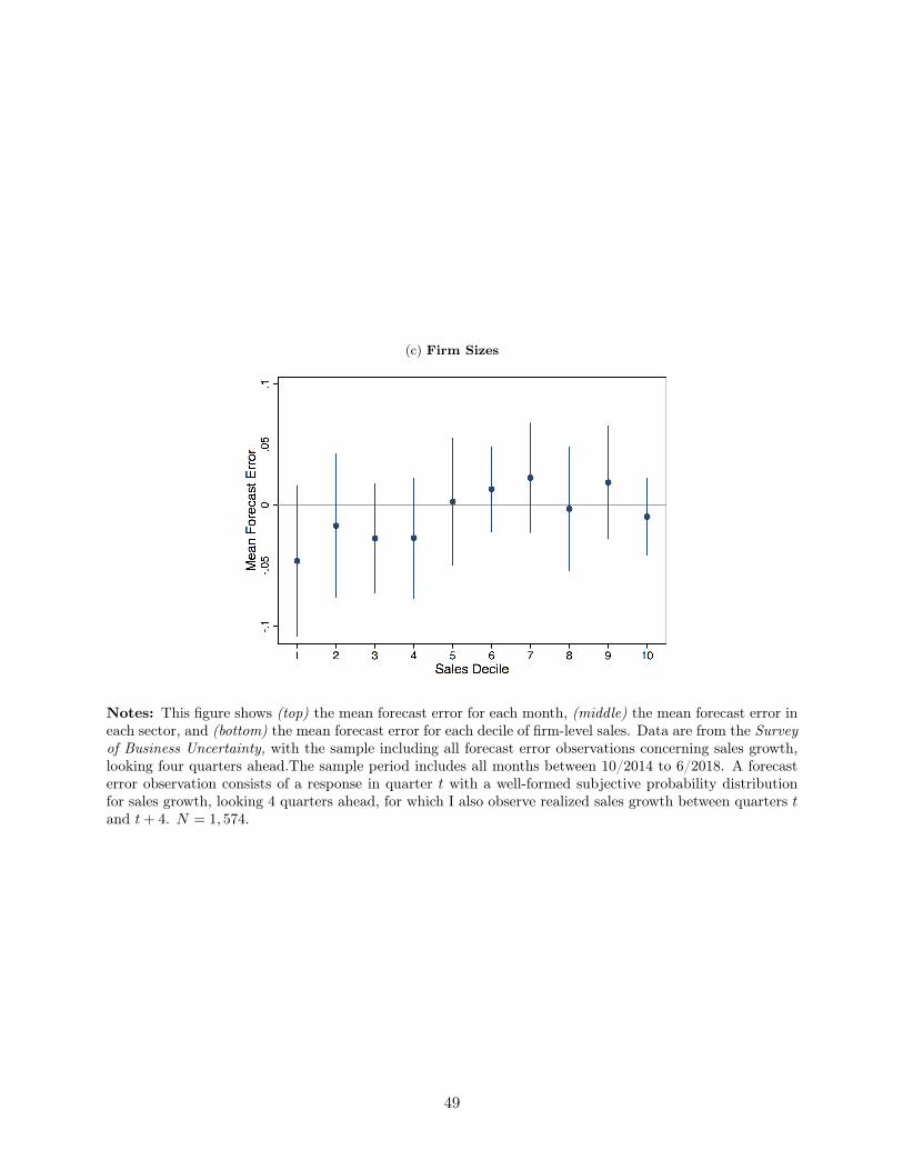
(c) Firm Sizes

Notes: This figure shows (top) the mean forecast error for each month, (middle) the mean forecast error ineach sector, and (bottom) the mean forecast error for each decile of firm-level sales. Data are from the Surveyof Business Uncertainty, with the sample including all forecast error observations concerning sales growth,looking four quarters ahead.The sample period includes all months between 10/2014 to 6/2018. A forecasterror observation consists of a response in quarter t with a well-formed subjective probability distributionfor sales growth, looking 4 quarters ahead, for which I also observe realized sales growth between quarters tand t+ 4. N = 1, 574.

49

Figure 5: Managers are Overconfident

Notes: This figure plots the empirical distribution of forecast errors as well as the distributionof forecast errors that would arise if sales growth realizations were drawn from SBU respondents’subjective probability distributions. I scale each distribution so that the sum of the heights of thebars is equal to one, and fix the width of the bars to 0.05. The sample period includes all monthsbetween 10/2014 to 6/2018. A forecast error observation consists of a response in quarter t with awell-formed subjective probability distribution for sales growth, looking 4 quarters ahead, for whichI also observe realized sales growth between quarters t and t+ 4. N = 1, 574.

50

Figure 6: Overconfidence Across Time, Sectors, and Firm Sizes

(a) Time

(b) Sectors

51

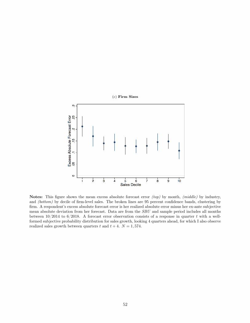
(c) Firm Sizes

Notes: This figure shows the mean excess absolute forecast error (top) by month, (middle) by industry,and (bottom) by decile of firm-level sales. The broken lines are 95 percent confidence bands, clustering byfirm. A respondent’s excess absolute forecast error is her realized absolute error minus her ex-ante subjectivemean absolute deviation from her forecast. Data are from the SBU and sample period includes all monthsbetween 10/2014 to 6/2018. A forecast error observation consists of a response in quarter t with a well-formed subjective probability distribution for sales growth, looking 4 quarters ahead, for which I also observerealized sales growth between quarters t and t+ 4. N = 1, 574.

52

Figure 7: Managers Overextrapolate from Current Conditions

Notes: This figure shows a bin-scatter of realized forecast errors for sales growth between t andt+ 4 on the vertical axis against realized sales growth between quarters t−1 and t, just prior to thesurvey response. Data are from the SBU and sample period includes all months between 10/2014 to6/2018. A forecast error observation consists of a response in quarter t with a well-formed subjectiveprobability distribution for sales growth, looking 4 quarters ahead, for which I also observe realizedsales growth between quarters t and t+ 4. N = 919.

Figure 8: Managerial Overextrapolation Across Firm Sizes

Notes: This figure shows the coefficients from regressing forecast minus realized sales growthbetween quarter t and t + 4 on the firm’s lagged sales growth from t − 1 to t separately for eachof five quintiles of the distribution of sales level. The horizontal bars are 95 percent confidenceintervals based on firm-clustered standard errors.

53

Figure 9: Net Hiring vs. Labor Productivity

Notes: This figure shows the joint distribution of log(labor productivity) on the horizontal axis andnet hiring on the vertical axis in my baseline economy with biases and a counterfactual economy inwhich all managers are unbiased. To construct the figure, I sort the stationary distribution of eacheconomy into 20 quantiles by log-labor productivity ratio and plot the mean labor productivity ineach quantile on the horizontal axis against the mean net hiring rate on the vertical axis.

54

Figure 10: Welfare Effects of a Tax on Hiring & Firing Expenditures

Notes: This figure shows the change in welfare across the steady state in an economy with a taxon hiring/firing expenditures relative to the baseline estimated economy. In both cases managersare biased. The curve shown uses a third-order polynomial to smooth out kinks due to numericalapproximation of equilibrium.

55

Table 1: Managerial Forecasts have Predictive Power

(1) (2) (3) (4) (5) (6)Dependent Variable Realized Sales Growth, t to t+4 Actual Hiring, t to t+4

Sales Growth Forecast, t to t+4 1.013*** 0.662**(0.147) (0.261)

Forecast (Planned) Hiring, t to t+4 0.718*** 0.715***(0.164) (0.105)

Sales Growth, t-1 to t -0.020 -0.037* 0.024 0.010(0.021) (0.019) (0.021) (0.020)

Net Hiring, t -0.056 -0.042 -0.243** -0.180(0.062) (0.054) (0.117) (0.112)

log(Cap. Expenditures), t 0.008** 0.008** 0.013** 0.011**(0.004) (0.004) (0.006) (0.005)

log(Employees), t -0.021** -0.021*** -0.017* -0.017*(0.009) (0.008) (0.010) (0.010)

Industry FE (14) Y Y Y YRegion FE (9) Y Y Y YAge FE (22) Y Y Y Y

Observations 517 517 1,313 609 609 1,604R-squared 0.452 0.523 0.160 0.241 0.310 0.142

Notes: Columns (1) to (3) regress actual sales growth between quarters t and t+4 on information availablein the quarter of the forecast. Columns (4) to (6) do the same for actual net hiring between t and t+4.I respectively include the respondent’s forecast for sales growth or net hiring to show it has significantpredictive power and its inclusion increases the marginal R-squared . I weight regressions by measures ofaccuracy for realized sales growth and actual hiring. Standard errors in parentheses, clustered by firm. Dataare from the SBU covering 10/2014 to 6/2018 collapsed to quarterly frequency. *** p<0.01, ** p<0.05, *p<0.1

56

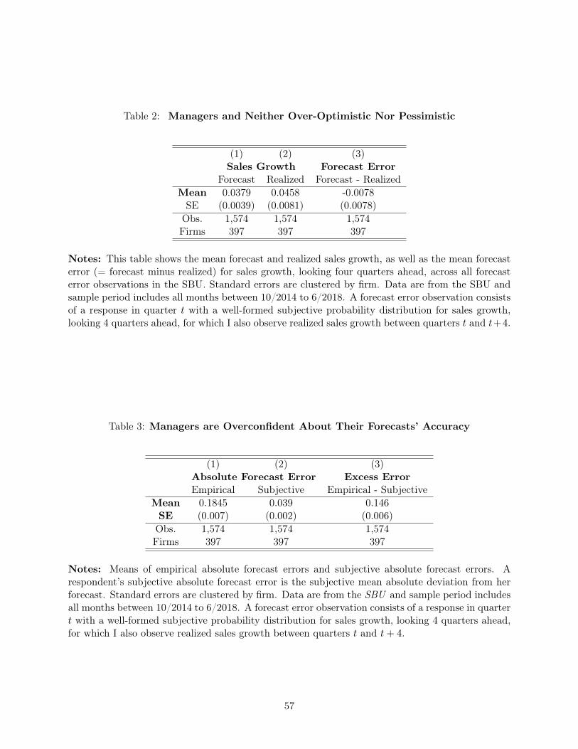
Table 2: Managers and Neither Over-Optimistic Nor Pessimistic

(1) (2) (3)Sales Growth Forecast Error

Forecast Realized Forecast - RealizedMean 0.0379 0.0458 -0.0078SE (0.0039) (0.0081) (0.0078)Obs. 1,574 1,574 1,574Firms 397 397 397

Notes: This table shows the mean forecast and realized sales growth, as well as the mean forecasterror (= forecast minus realized) for sales growth, looking four quarters ahead, across all forecasterror observations in the SBU. Standard errors are clustered by firm. Data are from the SBU andsample period includes all months between 10/2014 to 6/2018. A forecast error observation consistsof a response in quarter t with a well-formed subjective probability distribution for sales growth,looking 4 quarters ahead, for which I also observe realized sales growth between quarters t and t+4.

Table 3: Managers are Overconfident About Their Forecasts’ Accuracy

(1) (2) (3)Absolute Forecast Error Excess ErrorEmpirical Subjective Empirical - Subjective

Mean 0.1845 0.039 0.146SE (0.007) (0.002) (0.006)Obs. 1,574 1,574 1,574Firms 397 397 397

Notes: Means of empirical absolute forecast errors and subjective absolute forecast errors. Arespondent’s subjective absolute forecast error is the subjective mean absolute deviation from herforecast. Standard errors are clustered by firm. Data are from the SBU and sample period includesall months between 10/2014 to 6/2018. A forecast error observation consists of a response in quartert with a well-formed subjective probability distribution for sales growth, looking 4 quarters ahead,for which I also observe realized sales growth between quarters t and t+ 4.

57

Table 4: Managers Overextrapolate: Forecast Errors versus Recent Performance

(1) (2) (3) (4)Dependent Variable Forecast - Realized Sales Growth, quarters t to t+4

Sales Growth, quarters t− 1 to t 0.196*** 0.196*** 0.231*** 0.211***(0.039) (0.038) (0.040) (0.043)

Constant -0.018*(0.010)

Date FE Y YDate x Sector FE YFirm FE Y

Observations 919 919 869 862R-squared 0.059 0.092 0.254 0.451

Notes: This table regresses managers’ forecast minus realized sales growth between quarter t andt+4 on the firm’s sales growth between quarters t−1 and t. Robust standard errors in parentheses,clustered by firm. Data are subjective probability distributions and realizations for firm-specificsales growth looking four quarters ahead of the date of the forecast from the Survey of BusinessUncertainty. Data are from the SBU and sample period includes all months between 10/2014 to6/2018. A forecast error observation consists of a response in quarter t with a well-formed subjectiveprobability distribution for sales growth, looking 4 quarters ahead, for which I also observe realizedsales growth between quarters t and t+ 4. *** p<0.01, ** p<0.05, * p<0.1

58

Table 5: Externally-Calibrated Parameters

Parameter Value Description Target/Sourceq 0.08 Quarterly separation rate Shimer (2005)µ 0 Mean log(z) Normalizationγ 2 Inverse EIS Hall (2009)η 2 Inverse Frisch elasticity of lab. supply Chetty et al. (2011)β 0.961/4 Household discount factor Annual Interest Rate of 4%χ 29.7 Disutility of work Steady-state labor N∗ = 1/3θ 0.05 Managers’ share of equity Nikolov and Whited (2014)

59

Table 6: Structural Estimation Results

(a) Data and Model Moments

Moment Data ModelMean(Forecast Error) -0.013 -0.010

Mean(Excess Absolute Forecast Error) 0.143 0.129Cov(Forecast Errort,t+4, Sales Growtht−1,t) 0.011 0.008

Var(Sales Growth) 0.060 0.049Var(Net Hiring) 0.019 0.001

Cov(Net Hiring, Sales Growth) 0.003 0.004Cov(Sales Growtht,t+4,Sales Growtht−1,t) -0.012 -0.011Cov(Sales Growtht,t+4, Net Hiringt,t+1) -0.002 -0.004

(b) Estimated Parameters

Parameter Explanation Estimate (SE)α Revenue curvature 0.6132 (0.036)λ Quadratic adjustment costs 27.3 (0.800)ρ True shock persistence 0.801 (0.005)ρ Subjective Sshock persistence 0.913 (0.005)σ True shock volatility 0.212 (0.0006)σ Subjective shock volatility 0.098 (0.0006)µ Subjective shock mean -0.003 (0.00003)

Notes: This table shows the results from my structural estimation of the model from Section 3.Sub-table 6a (top) shows my target moments in the data and the corresponding model momentsafter choosing the vector of parameters that minimize the weighted distance between model and datamoments. I estimate all data moments using SBU data with the sample period covering 10/2014 to6/2018. All of the variances and covariances I target correspond to within-firm variation. Namely,before computing my target covariances and variances I regress all observations of a full set of firmand date fixed effects to purge variation due to aggregate shocks and persistent differences acrossfirms and then compute the variances and covariances on the residual of those regressions. I computemodel moments numerically from the stationary distribution of firms across the (z, n) state spaceof the model. Sub-table 6b (bottom) shows the values and standard errors of the parameters thatminimize the weighted distance between model and data moments. Note that I normalize the truemean of the stochastic process for log(z) to µ = 0. My choice of weighting matrix is the firm-levelclustered covariance matrix of SBU data moments, namely the GMM efficient weighting matrix.I perform the numerical optimization of the econometric objective using a simulated annealingalgorithm.

60

Table 7: Eliminating Beliefs Biases Increases Firm Value

Counterfactual ∆ True Firm Value (%)σ = σ only 0.4ρ = ρ only 1.3ρ = ρ, and σ = σ 1.9ρ = ρ, σ = σ, and µ = µ 1.9

Notes: This table shows how much firm value would increase by replacing a biased manager withanother who has fewer or no subjective beliefs biases, holding all else constant. At each pointin the (z, n) state space I compute the objective value generated by the biased managers in myestimated economy as well as the objective value generated by a counterfactual manager lackingpessimism (µ = µ), overconfidence (σ = σ), and/or overextrapolation (ρ = ρ). Then I compute themean percent gain in firm value by averaging the gains across the state space under the stationarydistribution of the economy with biases.

Table 8: Aggregate Impact of Beliefs Biases

∆ Consumer Welfare % ∆Y % ∆ (Y/N) %0.99 1.6 0.17

Notes: This table shows the difference in the household’s consumption-equivalent welfare, aggregateoutput (GDP), and labor productivity in the long-run equilibrium of an economy with unbiasedmanagers relative to the long-run equilibrium of my baseline economy with biased managers.

Table 9: Biases Encourage Excessive Reallocation

Reallocation ×100 σ(log(MPN)) AC/Y × 100

With Biases 5.7 0.33 16.6No Biases 1.1 0.35 14.4Difference -81.5% 6.6% -13.1%

Notes: This table compares steady-state values of the rate of reallocation (= total hiring and firing∆nt+1 as a fraction of total labor N), dispersion in the marginal product of labor, and aggregateadjustment costs paid as a share of aggregate output in my estimated economy with biases and inan efficient economy with unbiased managers. Y is aggregate GDP after subtracting output spenton adjustment costs. Both the baseline economy with biases and the counterfactual economy withno biases are in general equilibrium.

61

Table 10: Macro Impact of Individual Biases

Counterfactual ∆ C. Welfare % ∆ Realloc. % ∆σ(log(MPN)) % ∆AC/Y × 100

σ = σ only 0.28 -11.4 0.8 -0.3ρ = ρ only 0.68 -89.1 7.7 -2.5ρ = ρ and σ = σ 0.91 -79.6 6.4 -2.2ρ = ρ, σ = σ, and µ = µ 0.99 -81.5 6.6 -2.2

Notes: This table shows the difference in household consumption-equivalent welfare, reallocation,dispersion in the marginal product of labor, and adjustment costs as a share of GDP in the steadystate of an economy whose managers lack one or more of overconfidence (σ = σ), overextrapolation(ρ = ρ), or pessimism (µ = µ) relative to the steady state of my baseline economy with beliefsbiases. Both the baseline economy with biases and the counterfactual economies with no biases arein general equilibrium.

62

Tab

le11:Quan

titative

ResultsRob

ustness

(a)Micro

Cou

nterfactuals:

Makeasingleman

ager

unb

iased

∆TrueFirm

Value

(%)

Cou

nterfactual

Baseline

HighAdj.

Costs

Low

Adj.

Costs

Low

q

(sep

aration

rate)

Highα

Investment

Mod

el

σ=σon

ly0.4

0.2

0.2

0.1

0.7

0.4

ρ=ρon

ly1.3

0.6

1.0

1.5

3.2

2.8

ρ=ρan

dσ

=σ

1.9

0.7

1.5

2.1

5.5

3.0

ρ=ρ,σ

=σ,a

ndµ

=µ

1.9

0.7

1.5

2.1

5.5

3.0

(b)Macro

Cou

nterfactuals:

Makeallman

agersunb

iasedin

general

equilibrium

∆Con

sumer

Welfare

(%)

Cou

nterfactual

Baseline

HighAdj.

Costs

Low

Adj.

Costs

Low

q

(sep

.rate)

Highα

Highθ

(man

ager’s

equity)

Low

θ

(man

ager’s

equity)

Investment

Mod

el

σ=σon

ly0.28

0.26

0.14

0.29

0.32

0.50

0.21

0.18

ρ=ρon

ly0.68

0.38

0.48

0.68

1.13

0.59

0.70

-0.11

ρ=ρan

dσ

=σ

0.91

1.03

0.64

0.87

1.50

1.13

0.85

0.37

ρ=ρ,σ

=σ,a

ndµ

=µ

0.99

1.41

0.66

0.90

1.58

1.27

0.90

0.42

Notes:Tab

le11a(top)show

sho

wmuchfirm

valuewou

ldincrease

byreplacingabiased

man

ager

withan

othe

rwho

hasfewer

orno

subjective

belie

fsbiases,

holdingallelse

constant.Colum

nscorrespo

nsto

diffe

rent

mod

elspecification

s.Tab

le11b(bottom)show

sthechan

gein

consum

erwelfare

wewou

ldob

tain

from

movingto

acoun

terfactual

econ

omyin

which

allman

agersha

vefewer

orno

subjective

belie

fsbiases.Eachof

thesewelfare

chan

gescorrespo

ndto

acompa

rison

oftheaggregatesteady

stateof

theba

selin

eecon

omywithbiased

man

agersan

dtheaggregatesteady

stateof

thecoun

terfactual

econ

omyun

derconsideration.

The

baselin

ecolumnrefers

totheestimated

econ

omyin

from

SectionX.S

pecifications

withhigh

andlow

adjustmentcostsrespectively

have

threetimes

andon

ethirdmyestimated

adjustmentcost

parameterλ,w

hich

equa

ls27.3

intheba

selin

e.The

specification

withlow

sepa

ration

rateqsees

0.026of

thefirm’sworkforce

sepa

rate

exogen

ouslyeach

quarterdo

wnfrom

0.083in

theba

selin

e,correspo

ndingto

10pe

rcentan

nually

rather

than

30pe

rcentin

theba

selin

e.The

columns

labe

led"h

ighα

”im

pose

decreasing

returnsto

scaleon

theorde

rofα

=0.8,high

erthan

myba

selin

eestimated

valueofα

=0.61.Sp

ecification

swithhigh

and

low

man

ager’s

equity

shareθrespectively

triple

andcutby

athirdtheman

ager’s

equity

sharefrom

itsba

selin

elevelofθ

=0.0

5.(N

ote,θdo

esno

taff

ectthe

micro

coun

terfactualsin

Tab

le11a).Finally,thecolumnfortheinvestmentmod

elshow

sresultsfrom

amod

elin

which

labo

ris

chosen

statically

andcapitalis

subjectto

adjustmentcostswhich

Iestimateusingda

tafrom

theSu

rvey

ofBusinessUncertainty

aswella

sfrom

Com

pustat.Se

eApp

endixB.5

forade

scription

ofthis

mod

elan

dApp

endixC.7

forde

tails

onitsestimation.

63