THE METHOD OF SIMULATED ANNEALING FOR THE OPTIMAL ...
143
iii THE METHOD OF SIMULATED ANNEALING FOR THE OPTIMAL ADJUSTMENT OF THE NIGERIAN HORIZONTAL GEODETIC NETWORK BY O. G. OMOGUNLOYE MATRICULATION NUMBER: 840405039 Ph. D THESIS SUBMITTED TO THE SCHOOL OF POST GRADUATE STUDIES DEPARTMENT OF SURVEYING AND GEOINFORMATICS FACULTY OF ENGINEERING UNIVERSITY OF LAGOS AKOKA, LAGOS, NIGERIA October, 2010
Transcript of THE METHOD OF SIMULATED ANNEALING FOR THE OPTIMAL ...

iii
THE METHOD OF SIMULATED ANNEALING FOR THE OPTIMAL ADJUSTMENT
OF THE NIGERIAN HORIZONTAL GEODETIC NETWORK
BY
O. G. OMOGUNLOYE
MATRICULATION NUMBER: 840405039
Ph. D THESIS SUBMITTED TO THE
SCHOOL OF POST GRADUATE STUDIES
DEPARTMENT OF SURVEYING AND GEOINFORMATICS
FACULTY OF ENGINEERING
UNIVERSITY OF LAGOS
AKOKA, LAGOS, NIGERIA
October, 2010

iv
SCHOOL OF POSGRADUATE STUDIES UNIVERSITY OF LAGOS
CERTIFICATION
THIS IS TO CERTIFY THAT THE THESIS:
“THE METHOD OF SIMULATED ANNEALING FOR THE OPTIMAL ADJUSTMENT
OF THE NIGERIAN HORIZONTAL GEODETIC NETWORK”
SUBMITTED TO THE
SCHOOL OF POSTGRADUATE STUDIES
UNIVERSITY OF LAGOS
FOR THE AWARD OF THE DEGREE OF
DOCTOR OF PHILOSOPHY (Ph. D) IS A RECORD OF ORIGINAL RESEARCH CARRIED OUT
BY
OMOGUNLOYE, OLUSOLA GABRIEL IN THE DEPARTMENT OF SURVEYING AND GEOINFORMATICS
----------------------------------------- ------------------------- -----
----------
AUTHOR‟S NAME SIGNATURE
DATE
---------------------------------------- ------------------------- ----
-----------
1ST
SUPERVISOR NAME SIGNATURE
DATE
----------------------------------------- ------------------------- -----
----------
2ND
SUPERVISOR NAME SIGNATURE
DATE
----------------------------------------- ------------------------- -----
----------

v
3RD
SUPERVISOR NAME SIGNATURE
DATE
----------------------------------------- ------------------------- -----
----------
1ST
INTERNAL SUPERVISOR SIGNATURE
DATE
----------------------------------------- ------------------------- -----
----------
2ND
INTERNAL SUPERVISOR SIGNATURE
DATE
----------------------------------------- ------------------------- -----
----------
EXTERNAL EXAMINAR SIGNATURE
DATE
----------------------------------------- ------------------------- -----
----------
SPGS REPRESENTENTIVE SIGNATURE
DATE
vi
ABSTRACT
The Horizontal Geodetic Network of Nigeria is made up of terrestrially arranged chains of
triangles augmented by precise traverses. The work on the network began early 19th century
but by 1930 the work was discarded and a re-observation of the network was carried out to
the highest possible accuracy then, enhanced with high order geodimeter traverses which
linked to other neighboring African networks.
The full network consists of 515 stations, with 2411 observations which comprise 2197 angular
observations, 40 Laplace azimuths and 174 measured distances, part of which substituted for
the sparse triangulation observations especially in the southern part of the country. The added
observations contributed to strengthening of the network in the 1977 adjustment which
however was not a holistic optimized adjustment, but rather, a phase adjustment. Based on the
1977 state of adjustment of the network, no meaningful distortion monitoring exercise can take
place until the network is adjusted by an optimized simultaneous technique in order to
ascertain the state and consistency of the network.
The use of the simulated annealing method, which has been successfully applied in other fields,
is presented for the classical geodetic problem of simultaneous adjustment of the entire
triangulation net using the least squares observation equation method. This method is an
iterative heuristic technique (a method of solving problems by learning from past experience
and investigating practical ways of finding a solution) in operations research. It uses a thermo
dynamic analogy (Cooling theory) to adjust a network of unstable stations (changes to gaseous
state) through fairly stable station coordinates (liquid state) to a stable station coordinates
(solid state) so as to offer a solution that converges in a probabilistic sense (statistically based)
to the global optimum. The simulated annealing method of optimization serves to help
determine the position of all triangulation stations by means of minimizing the volume of the
error hyper ellipsoid inherent in the solution to give an optimal configuration of the geodetic
network. Computer programs were developed using Matlab Software and run on an adequately
configured Pentium IV computer. Creation of an intelligent database was achieved through the

vii
interactive network of the data storage, processing, manipulation, analysis and retrieval of
results of the adjustment.
The result of the new adjustment produced a generally consistent trend of changes in the
distances and azimuths compared to the previous adjustments. Error analysis of all lines were
carried out and the respective standard errors in distances and azimuths were determined.
Relative and absolute error ellipses of all stations were determined and plotted. Statistical plots
and analysis of the error ellipses of the network stations were also determined. The absolute
and relative weakness/strength of the network stations coordinates after adjustment were
shown and confirmed by the error plots to have the following geometry error distributions.
That is, 90.5% of the 515 Network Stations fell within Network Standard deviation of 1- Sigma,
94.2% within 2-Sigma, while 98.3% fell within 3- Sigma
The distributions confirmed the high reliability of the Nigerian Horizontal Geodetic Network and
its data quality. Re-strengthening exercise would be necessary using either the 1-Sigma or 2-
Sigma region of network standard deviation
A data structure for the entire network was developed and necessary conclusions and
recommendations are made for further action to update/upgrade the precision of the Nigerian
horizontal geodetic network for future study.
Keywords: Geodetic network, Optimum adjustment, Simulated annealing technique, Least
squares technique.

viii
DEDICATION
This work is dedicated to The Living Word of God that made all things (John 1:1-5), Who is the
True Light that gives Light to Every man coming into the world (John 1:9), Who also is the
Alpha and Omega, the First and the Last (Revelations 1:11a), Who became flesh and dwelt
among us (John 1:14), Who is the Lamb of God Who took away the sins of the world (John
1:29), Who died for our sins (Romans 5:8), Who has a name above all names (Philippians 2:9),
Who has all authority in Heaven, on Earth and Under the Earth (Matthew 28: 18), Who is the
soon coming King, with rewards (Acts 1:11, Revelations 22:12), Who is therefore the KING OF
KINGS AND THE LORD OF LORDS (Revelations 19:16) – HIS NAME IS JESUS CHRIST.
THANK YOU LORD JESUS CHRIST - MY SAVIOR AND MY LORD
KEEP ME SAVED TILL YOU COME.

ix
ACKNOWLEDGEMENT
My greatest thanks go to the FATHER, SON AND THE HOLY SPIRIT for giving me the grace to
begin and complete this research work, which without doubt is a milestone accomplishment in
my life and in the nation (Nigeria) at large. The journey so far has been possible because His
presence has been continuously abundant in my life. The required knowledge, wisdom and
understanding for the fulfillment of this work had been solely from Him.
I will not be justified if at this state, I fail to acknowledge my spiritual and academic father as
well as my supervisor, Professor O.O. Ayeni and his wife (mummy). You have fully guided,
assisted, supported and encouraged me from the beginning of this research to the end, indeed
you are my God-sent angel, may the good Lord continue to uphold you and your family, thanks
uncountable times.
I am highly indebted to Professor J.B. Olaleye who by the abundant grace of God upon his life
became not only a leader but a father to everyone of us in the department. Your constructive
criticism and intellectual eagle eyes had contributed and added to the beauty and the eventual
accomplishment of this research work. May the good Lord always remember your labor of love
in Jesus name.
The technical aspect of this research work had been enhanced by my supervisor, Professor P.C.
Nwilo, who has stood his ground to criticize, correct and perfect the technical inputs in this
work. You always have riddles to pose that would assist one to determine to rise up in life.
Thank you very much sir.
My profound thanks go to Professor F.A. Fajemirokun, Professor Ezeigbo and late Professor
F.O. Egberongbe who during the period of my academic pursuit had contributed immensely to
this study. Thank you very much sirs.
My sincere thanks go to my academic fathers – Prof V.O.S. Olunloyo, Prof. O. Ibidapo - Obe,
Professor Olu Ogboja (late), Professor A. B. Sofoluwe (The Vice Chancellor), Professor M.A.
Salau (Dean of Faculty of Engineering), Professor O. T. Ogundipe (Dean of PG School). May the
good Lord continually bless and make you a blessing on earth.

x
Dr. J.O. Olusina (H. O. D., Department of Surveying and Geoinformatics) and Dr. O.T. Badejo
(Department of Surveying and Geoinformatics PG Coordinator), you are among the very few
that showed interest in my work by correcting and suggesting constructive ideas that brought
about the completeness of this work. Thanks a million times.
The accomplishment of this work has majorly been realized as a result of the cooperation of my
beautiful wife, MRS. HANNAH GOODNESS, ENIOLA OMOGUNLOYE, who had paid all the
utmost prize of a mother to my children through the period of this research, especially when I
had to pitch my tent in my office to be able to complete the work. She particularly showed a
rare asset of weathering all the storms of life with me especially during our rough financial
days. I pray I would be gracefully placed to reward your labor of love, thank you very much
I will, at this time, acknowledge MY BEAUTIFUL CHILDREN LIGHT OREOLUWA (LIGHTOO),
TRUTH GBOLAHAN (TRUTHEE), PEACE OTARU (PEACEE) AND PRAISE JESUS (PRAISOO), You
have all been wonderful, beautiful, great and glorious children. You are all blessed in Jesus
name.
Big thanks to Surveyor Lola (you assisted me and the Nation Nigeria to recover the lost data
for this research), Surveyor J.T. Ajayi, Mr. A.O. Adebisi, Mr. H. Mosaku, Mr. E.E. Epuh, Mr. O.E.
Abiodun, Mr. E.G. Ayodele, Mrs. A.M. Ayeni (Pastor), Mr. A. Alademomi, Surveyor M. Jegede,
Surveyor R. Adekola, Surveyor O.A. Babatunde, Ms. G.I. Inyang, Mrs. C.A. Sokenu, Mr. D.J.
Ikechukwu, Mrs. M.A. Adeyinka, Mr. O. Omojowo, Mrs. K. Sulaimon, Mrs. A. Ekanem, Mr
Adebayo, Mr Iluyemi, Brother Oshode Joseph Olusola, Mr. R. Adeyeye, Mr. Lawal, Alhaji
Jimoh, Alhaja Okonu, Mr. Oluga, Mr. Thomas, Mr. Durojaiye (late) and Mr. Ojo (late), I
appriaciate all your contributions
Associate Professor G.O. Oyekan (Daddy), and Professor D. E. Esezobor - I acknowledge your
concern for people’s progress and welfare. Dr. Adeosun, Dr. Ladi Ogunwolu, Dr. Fashanu, Dr.
Akanmu, Associate Professor Ayesimoju, Dr Kamiyo, Dr. S. Ojolo, Brother Joel, and Mummy
A. Sholiyi, thanks for all your supports and encouragements at all times. Pastor Taiye Adeoye,
Pastor F.A. Festus, thanks for your support.

xi
I say thank you to Pastor S.O. Adefarakan, Dr. (Mrs.) T.F. Ipaye, Mrs Ogunlewe, Miss Bimbo
Komolafe and Mr. Kingsley Okhiria, all of PG school, for all your persistent readiness to help,
assist, encourage, and attend to researchers, the Lord will crown all your efforts with success.
I appreciate my God Given Spiritual Children – Evangelist Yinka Akinsulire, Evangelist Elijah
Omogunloye, Evangelist Alaba Omogunloye, Brother Seun Adebayo (late – rest in peace),
Brother Wale Arowoiya, Brother Anuoluwa Ojemuyiwa, Brother Opeyemi Ayorinde, Pastor
Sunday Omogunloye, Pastor Idowu Omogunloye, Evangelist Emily Omogunloye, Deaconness
Lawal and the members of Jesus The Light, Word Outreach Ministries – You are all blessed in
Jesus Name. Thanks to Engineer and Mrs. B. R. Owolabi for all your support.
My elder sister (Mrs. Bukonla Emuleomo), her husband (Rev. Bayo Emuleomo) and Children;
Mr. Banji Omogunloye, his wife (Mummy Tops) and Children; Pastor Gbenga Omogunloye, his
wife (Mummy Dan) and children; my late brother Mr. Segun Omogunloye (rest in the bosom
of our Lord Jesus); Mrs. Kemi Adeoye and her wonderful family; Sister Funke Omogunloye;
Brother Dami; Brother Femi; Brother Deji; Sister Seye; and Brother Tobi - You’ve all been life
giver to me and my family. The good Lord will perfect all that concerns you in Jesus name.
I must not forget my in-laws - late Mr. Enesi (daddy), Mummy Sango (My mother in-law)
Reverend Dr. Peter Enesi, Sister Victoria, Reverend Abraham, Brother Godwin, Sister Bose,
Brother Lucky, Brother Johnson and your respective nuclear families – I love you all; you’ve
been so dear to me.
Finally to my Dear father, Pastor J.A. Omogunlye and my precious mother, Mrs. B.I.
Omogunloye, you have been there for me from pregnancy throughout my study days till date.
You have been an example of a good parent on the earth. The good news is that, Daddy, though
you are a carpenter and mummy, a trader, but you have a Ph.D holder as a son –
CONGRATULATIONS.
In conclusion, LORD JESUS, I return all the glory, honor, and majesty to you, for without you, we
can do nothing and by strength shall no one prevail.

xii
TABLE OF CONTENTS PAGE
CONTENTS
Title Page i
Certification ii
Abstract iii
Dedication v
Acknowledgement vi
List of Figures xiii
List of Tables xv
List of Appendices xvii
Glossary of Notations and Abbreviations xix
`
CHAPTER ONE: INTRODUCTION
1.1 Background of the Study 1
1.1.1 Previous Adjustments 2
1.2 Statement of the Problem 5
1.3 Aim and Objectives of the Research 6
1.4 Scope and Limitations of the Research 6
1.5 Significance of the Research 7
1.6 Research Questions 7
1.7 Definition of Operational Terms 8

xiii
CHAPTER TWO: GEODETIC NETWORK
2.0 Literature Review 11
2.1 Theoretical Framework 25
2.1.1 Computations of Geodetic Coordinates on the Ellipsoid 25
2.1.1.1 Direct Problem Equations 26
2.1.1.2 Indirect Problem Equations (Inverse Problem) 28
2.1.2 Observation Equations on the Ellipsoid 30
2.1.3 The Least Squares Method 32
2.1.3.1 Simultaneous Method 33
2.1.3.2 Sequential Method 35
2.1.3.3 Phase Method 37
2.1.3.4 Combined (Phase and Sequential) Method 40
2.1.4 Network Geometry Assessment 42
2.1.5 FGCC Standard and Specification for Geodetic Control Networks 43
2.1.5.1 Standards 43
2.1.5.1.1 Horizontal Control Network Standards 44
2.1.5.1.2 Monuments 45
2.1.5.2 Specifications 45
2.1.5.2.1 Triangulation 45
2.1.5.2.2 Instrumentation 46
2.1.6 Definition of Best Geometric Configuration 48
2.1.6.1 W hat is Optimization 50
2.1.6.2 Optimization Techniques 52
xiv
CHAPTER THREE: METHODOLOGY
3.1 General 55
3.1.1 Data Acquisition 55
3.1.2 Data Pre – processing and Quality Control 57
3.1.2.1 Instruments used/Date of Observation 57
3.1.3 Data Processing 57
3.2 Simulated Annealing Algorithm 58
3.2.1 Least Squares Equations Part 58
3.2.2 Equations used for the Optimization Part 60
3.3 Error Ellipse 66
CHAPTER FOUR: RESULTS AND ANALYSIS
4.1 Result 72
4.1.1 The Recovered Network Data Format 73
4.1.1.1 Network New Data Structure Format 73
4.1.1.2 Instruments used/Date of Observation of Network 74
4.1.2 Residuals Vector (V) after Adjustment 77
4.1.3 Stations Positional Corrections 80
4.1.4 Error Ellipse (Geometry) Computation 83
4.1.5 Relative Error Ellipse (Relative Geometry) computation 86
4.1.5.1 Standard Error in Azimuths (Orientation) computation 88
4.1.5.2 Standard Error in Distances (Scale) computation 91
4.2 Analysis of Results 94
4.2.1 Analysis of the Network residuals of Observations (V) after the Adjustment 94
4.2.2 Analysis of the Network Stations Position Correction (x) after the adjustment 95

xv
4.2.3 Analysis of the Network Error Ellipse (Geometry) after the Adjustment 96
4.2..4 Analysis of the Network Relative Error Ellipse (Relative Geometry) 98
4.2.4.1 Analysis of the Network Standard Error in Azimuths (Orientation) 98
4.2.4.2 Analysis of the Network Standard Error in Distances (Scale) 98
4.2.4.3 Analysis of Network Standard Deviation 99
4.2.5 Statistical Paired Sample Test analysis of the error ellipse values of the 33
stations in 1977 and their corresponding values in 2009 adjustment. 100
4.2.6 Comparison of the 515 Stations Coordinates in the 1977 102
and 2009 Adjustments.
4.2.7 The summary of the Results in 1977 and 2009 Adjustments 105
CHAPTER FIVE: CONTRIBUTIONS TO KNOWLEDGE, CONCLUSIONS AND
RECOMMENDATIONS
5.1 Conclusion 106
5.2 Contribution to Knowledge 110
5.3 Recommendation/Further research Work 110
REFERENCES 112

xvi
LIST OF FIGURES PAGE
Figure 1.0 Graphical plot of Nigerian Horizontal Geodetic Network 4
Figure 2.1.1 Ellipsoidal Polar Triangles 26
Figure 2.1.2 Sample Triangle 30
Figure 2.1.3a Network View for the Simultaneous Method 34
Figure 2.1.3b Network view for the Sequential Method 36
Figure 2.1.3c Network view for the Phase Method 39
Figure 2.1.3d Network view for the combined (Phase and Sequential) Method 41
Figure 3.1 Plot of Cooling Scheme 63
(Gradual Stabilization of Network Coordinates)
Figure 3.2 Plot of Function of Free Movement Structure 64
Figure 3.3 Plot of Standard Deviation of Network Correction Vector 65
Figure 3.4 Graph of Standard Ellipse 69
Figure 4.1a Sample Triangular Structure 74
Figure 4.1.2a Plot of V matrix vector in the Network 79
Figure 4.1.2b Plot of V matrix of some CFL lines/type of Observation 80
Figure 4.1.2c Plot of V matrix of the of the first 7 Network Triangles 80
Figure 4.1.3a Plot of Positional corrections of 515 stations in the Network 82
Figure 4.1.3b Plot of the XL and ML Secondary Stations with Large 82
Positional Corrections
Figure 4.1.4a Plot of Network Stations with Larger Absolute Error Ellipse Sizes 85
Figure 4.1.4b Plot of Network CFL Stations with Large Absolute Error Ellipse Sizes 85
Figure 4.1.4c Plot of Network ML Stations with Larger Absolute Error 86
Ellipse Size

xvii
Figure 4.1.5a Plot of Network Stations with Larger Relative Error Ellipse Sizes 88
Figure 4.1.5b Plot of Network Standard Error Vector (S.e) in 90
Azimuhs (orientation)
Figure 4.1.5c Plot of the Network CFL Stations Cross Sectional view Standard 90
Error (S.e) in Azimuhs.
Figure 4.1.5d Plot of the Network XL and ML Stations Cross Sectional 91
View Standard Error (S.e) in Azimuths.
Figure 4.1.5e Plot of Network Standard Error Vector (S.e) in Distances (Scale) 93
Figure 4.1.5f Plot of the Network CFL Stations Cross Sectional view Standard 93
Error (S.e) in Distances
Figure 4.1.5g Plot of the Network XL and ML Stations Cross Sectional 94
View Standard Error (S.e) in Distances
Figure 4.2.5a Plot of the Paired Sample Test Results of the Absolute Error 102
Ellipses of 33 stations in the 1977 and 2009 at 95% Confidence Level
Figure 4.2.6a Plot of the Optimized Adjusted Horizontal Geodetic 104
Network of Nigeria

xviii
LIST OF TABLES PAGE
Table 2.0 (a) Invar Taped Baselines 12
Table 2.0 (b) Old Azimuths (Pre-1945) 13
Table 2.0 (c) The Nigerian Triangulation Network 15
Table 2.0 (d) Coordinates of Minna Datum L-40 computed from astromical
Observation stations in widely separated areas. 19
Table 2.0 (e) Comparison of GNSS Systems 25
Table 2.1.5.1.1 Distance Accuracy Standards 44
Table2.1.5.1.2 Network Geometry 46
Table 2.1.5.1.3 Instrument Order and Class 47
Table 2.1.5.1.4 Theodolite Observation 47
Table2.1.6.1 Summary of Optimization Solution Method 53
Table 3.1a Sample Angular Data 56
Table 3.1b Sample Azimuths Data 56
Table 3.1c Sample Scale check Data 56
Table 4.1a Sample Triangular Arranged Stations ID of the Network 73
Table 4.1b Sample Triangular Arranged Lines of the Network 73
Table 4.1c Sample Triangular Arranged Angles of the Network 74
Table 4.1d Instrument used for the Nigerian Horizontal Geodetic Network 75
Table 4.1e Sample Network Assessment based on Instruments and year 76
of Observation
Table 4.1.2a Results of the Sample Network Residual Vector (V) 78
after adjustment
Table 4.1.3a Results of the Sample Network stations Positional Corrections 81

xix
Table 4.1.4a Result of Sample Network Error Ellipse Computation 84
Table 4.1.5a Results of Sample Network Relative Error Ellipse Computation 87
Table 4.1.5b Results of Sample Network Standard Error in Azimuths 89
Computation
Table 4.1.5c Results of Sample Network Standard Error in Distances 92
Computation
Table 4.2.4.3a Classification/Assessment of Network A-Posteriori Variances 99
of unit weight
Table 4.2.5a Comparison of Error Ellipse Sizes for 33 Stations used 101
in 1977 and 2009 Adjustment
Table 4.2.5b Statistical Paired Sample-Test on the Extracted Absolute 102
Error Sizes of 33 stations in 1977 and 2009 Adjustment
Table 4.2.6a Comparison of the Sample of Final Adjusted coordinates in 103
1977 and 2009
Table 4.2.7a Comparison of the Summary of 1977 and 2009 Adjustments 105

xx
LIST OF APPENDICES PAGE
Appendix (I a) Print of the Network Observed Angles (Now in soft copy) 123
Appendix (I b) Print of the Network Observed Azimuths (Now in soft copy) 129
Appendix (I c) Print of the Network Observed Distances (Now in soft copy) 130
Appendix (I d) The Programs written for the entire Research in Matlab 134
Appendix (II a) 1054 Triangular Arranged Network Stations Identity (ID) 148
Appendix (IIb) 1054 Triangular Arranged Network Lines/Stations Identity (ID) 155
Appendix (IIc) 1054 Triangular Arranged Network Observed Angles 162
Appendix (III) 3162 Network Residual Matrices Vector 169
Appendix (IV) 515 Network Stations Positional Corrections 189
Appendix (V) 515 Network Stations Error Ellipses Values (Network Geometry) 193
Appendix (VI) 3162 Network Lines/Stations Relative Error Ellipses Values 196
(Relative Geometry)
Appendix (VII) 3162 Network Standard Error in Azimuths of Lines (Network Orientation) 216
Appendix (VIII) 3162 Network Standard Error in Distances of Lines (Network Scale) 236
Appendix (IX) Comparison of the Final Coordinates in 1977 and 2009 Adjustment 256
(Stations Correction)
Appendix (X) Assessment of Instruments and Date of Observation of the Network 275
Appendix (XI a) Plot of Error Ellipses for all Chains/Stations in the Network 278
Appendix (XI b) Plot of Error Ellipses for A, some ML and XL Chains/Stations 279
Appendix (XI c) Plot of Error Ellipses showing the Weakness of the CFL Chain/Stations 280
Appendix (XI d) Plot of Error Ellipses showing the Western end of the CFL Chain/Stations 281
Appendix (XI e) Plot of Error Ellipses showing the Central part of the CFL Chain/Stations 282
Appendix (XI f) Plot of Error Ellipses showing the Eastern end of the CFL Chain/Stations 283
xxi
Appendix (XI g) Plot of Error Ellipses for D, and L Chains/Stations 284
Appendix (XI h) Plot of Error Ellipses for A, B, C, E, F, H, M, N, X, XL, ML and MR 285
Chains/Stations
Appendix (XI i) Plot of Error Ellipses for B, E, H, K, N, and P Chains/Stations 286
Appendix (XI j) Plot of Error Ellipses for A, E, F and G Chains/Stations 287
Appendix (XI k) Plot of Error Ellipses for K, and A part of the CFL Chains/Stations 288
Appendix (XI l) Plot of Error Ellipses for D, L and a part of U Chains/Stations 289
Appendix (XI m) Plot of Error Ellipses for C, F, H and M Chains/Stations 290
Appendix (XI n) Plot of Error Ellipses for A, E, F, G, XL, and ML CFL Chains/Stations 291
Appendix (XI o) Plot of Error Ellipses for B, K, N and A part of the CFL Chains/Stations 292
Appendix (XI p) Plot of Error Ellipses for C, H, M, P and U Chains/Stations 293
Appendix (XI q) Plot of Error Ellipses for R, CFL , XL Chains/Stations 294
Appendix (XI r) Plot of Error Ellipses for P and U Chains/Stations 295
Appendix (XI k) Plot of Error Ellipses for P and U Chains/Stations 296
Appendix (XII a) 49 Stations with Standard Error > 1 sigma that needs re-observation 297
Appendix (XII b) 30 Stations with Standard Error > 2 sigma that needs re-observation 298
Appendix (XII c) 9 Stations with Standard Error > 2 sigma that needs re-observation 299

xxii
GLOSSARY OF NOTATIONS AND ABBREVIATIONS
IAUE
Iterated Almost Unbiased Estimator
(LA-LG) Laplace correction
(C ) The computed value of an angle, azimuth, or distance
(O) The observed value of an angle, azimuth, or distance
A12 Azimuth of station 1 to 2
ACO Ant Colony Optimization
Ai j Azimuth of geodesic from i to j
ATPA Normal Matrix (N)
AZo The normal defined by the actual gravity vector
BA Bacteriologic Algorithms
CE Cross-entropy
The Stochastical covariance matrix model
D.F Degree of freedom
Correction to the direction from a normal section to geodesic.
Correction to the direction for the height of the observed point
D2 The corrected azimuth (Total direction correction)
The correction for the deflection of the vertical
Di j Length of geodesic from i to j
DOS. Directorate of Overseas Surveys
dφ, dλ, The change in latitude, longitude between two points
E1, E2 Easting of the ends of the line
EDM. Electromagnetic Distance Measurement
EO Extremal Optimization
EP Evolutionary Programming
ES Evolution Strategies
GGA Grouping Genetic Algorithm
GP Genetic Programming
xxiii
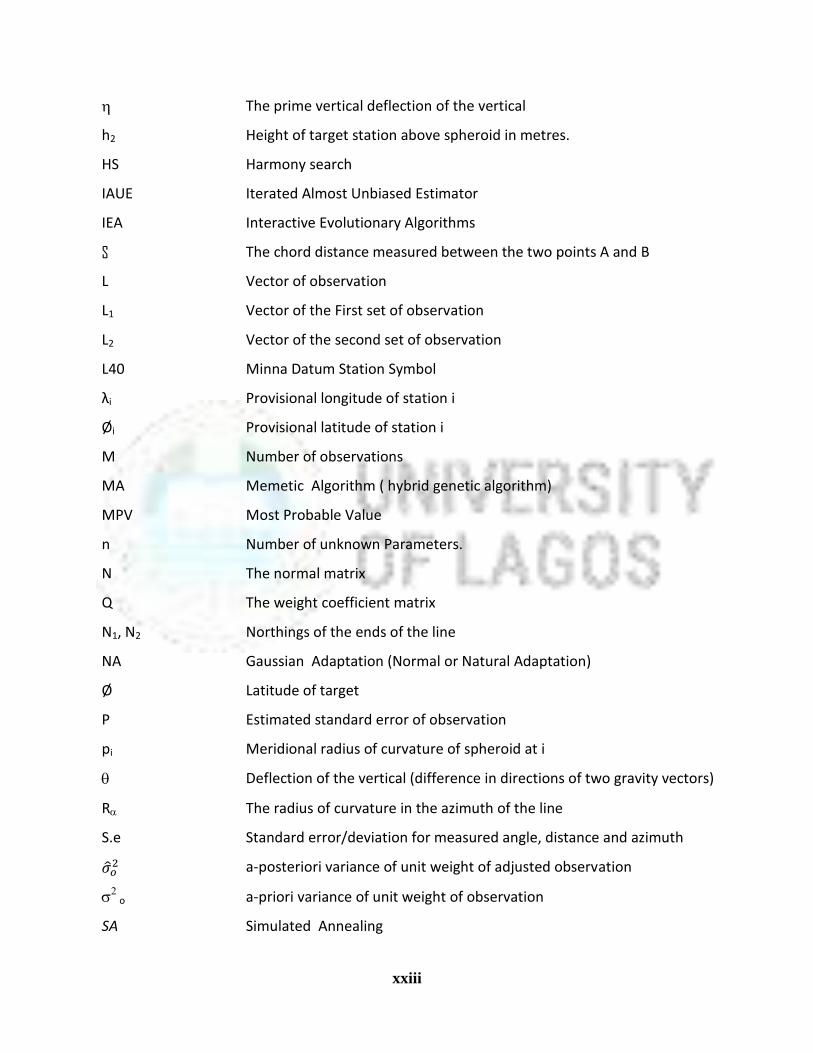
The prime vertical deflection of the vertical
h2 Height of target station above spheroid in metres.
HS Harmony search
IAUE Iterated Almost Unbiased Estimator
IEA Interactive Evolutionary Algorithms
S The chord distance measured between the two points A and B
L Vector of observation
L1 Vector of the First set of observation
L2 Vector of the second set of observation
L40 Minna Datum Station Symbol
λi Provisional longitude of station i
Øi Provisional latitude of station i
M Number of observations
MA Memetic Algorithm ( hybrid genetic algorithm)
MPV Most Probable Value
n Number of unknown Parameters.
N The normal matrix
Q The weight coefficient matrix
N1, N2 Northings of the ends of the line
NA Gaussian Adaptation (Normal or Natural Adaptation)
Ø Latitude of target
P Estimated standard error of observation
pi Meridional radius of curvature of spheroid at i
Deflection of the vertical (difference in directions of two gravity vectors)
R The radius of curvature in the azimuth of the line
S.e Standard error/deviation for measured angle, distance and azimuth
a-posteriori variance of unit weight of adjusted observation
o
a-priori variance of unit weight of observation
SA Simulated Annealing

1
SO Stochastic Optimization
The unbiased estimate of the convariance matrix of adjusted parameters
Trace (Ʃʟа) Trace of the variance covariance matrice of the adjusted observation
Trace (Ʃxа) Trace of the variance covariance matrice of the adjusted parameters
TS Tabu search
V The vector of residuals
vi Radius of curvature at right angles to meridian at i
Vi j k Residual of the observation at station ijk.
vTpv Sum of the squares of the residual
W Weight matrix
Xa Vector of the unknown adjusted parameter
X Vector of the correction to unknown Parameter
The meridian deflection of the vertical
Xo The approximate values of the unknown parameters
Zo The astronomic zenith
Ϭx Error Ellipse Parameter (Semi Major Axis)
Ϭy Error Ellipse Parameter (Semi Minor Axis)
Ψ Error Ellipse Parameter (Orientation of Ellipse)
La Adjusted observation (Angles, Distances and Azimuth)
F(La) Function of the adjusted observation (Angles, Distances and Azimuth)
Lb Vector of unadjusted observation
F(Xa) Function of adjusted Parameter
Xo1 1st set of approximate solution vector of Parameter
Xo2 2nd set of approximate solution vector of additional Parameter
Xa2 2nd set of Adjusted solution vector of additional Parameters
Xo Approximate Vector of the Parameter.

2
CHAPTER ONE
INTRODUCTION
1.1 BACKGROUND OF THE STUDY
A Geodetic Control network is a collection of identifiable stable points on the surface of the
earth tied together by observations of high accuracy. From these observations, the positional
coordinates of points are computed and published. This framework of coordinated point provides
a common basis for all surveying and mapping operations in a suitable reference system (Anon,
1971; Alliman and Hoar, 1973).
There are three National Geodetic Control frameworks, namely:
Horizontal Control framework, which is the focus of this study;
Vertical Control framework and;
Gravity Control framework;
The Nigerian Horizontal Geodetic Network is a network of terrestrial points made up of
triangulation, trilateration and traversing sub-networks, a larger part of which was observed
between 1930 and 1960. The thickly vegetated terrain of the southern part of Nigeria made the
use of triangulation method a difficult task, hence a system of Primary Traverses formed the
position control between 1923 and 1940 with later addition of microwave EDM traverses in the
south east. From 1960 to 1968, series of primary traverses were used to extend the triangulation
in the northern part of Nigeria, such as: the Trans-Africa Twelfth Parallel Geodimeter traverse
carried out by the U.S. Corps of Engineers which connected the triangulation at eight points; a
number of mapping projects were also carried out shortly after independence; controls provided
by aero triangulation were integrated into the network to fill many gaps between the main
triangulation chains; and additional scale and azimuth measurements were made to strengthen
the entire triangulation network (Anon, (1936 and 1961); Close, (1933); De Normann, (1933);
Dept. of the Army, (1953)).
The 1977 adjustment of the network, which integrated all the stations was a phase adjustment,
hence inadequate for a holistic optimal solution of the Nigerian Horizontal Geodetic Network.

3
Consequently, there is a need to implement a holistic optimal adjustment that will minimize the
volume of the error hyper ellipsoid inherent in the solution to give an optimal configuration of
the network.
This study shall comprise:
brief review of literatures on the Geodetic Network of some countries,
models used in adjustment of horizontal geodetic networks.
methods of holistic optimization using the Simulated Annealing Method.
results and analysis of results.
conclusions, contribution to knowledge and recommendations based on the outcome of the
research or study.
The end products of these work would assist in giving an optimal set of coordinates of stations in
the network which are often used directly or indirectly for:
Planning and carrying out national and local projects.
Development delineation of state and international boundaries.
Utilization of natural resources.
National defense, land management and monitoring of crustal motion.
Supporting the conduct of public business at all levels of government.
General basis of nationwide surveys, maps, and charts of various kinds (Chedtham, 1965;
Clark, 1965; Alliman and Hoar, 1973; Clark, 1965; Charles, 1942; Dare, 1995; Choi, 1998).
1. 1.1 Previous Adjustments
The network had been adjusted by some researchers and agencies. The first adjustment carried
out between 1930 and 1940 by the Directorate of Overseas Surveys was not completely
satisfactory due to misclosures between base and azimuth checks (Field, 1977). Another
adjustment by the U.S. Topocom used 440 existing stations and some observations made up to
1968. It excluded the 12th
Parallel Traverse (Field, 1977). Other adjustments between 1968 and
1977 were made on individual parts of the network, such as the Primary Traverses, which were
adjusted to connect the triangulation at eight points. The 12th
Parallel Traverse which was earlier
4
adjusted to a different origin but same spheroid (Clarke 1880), was re-adjusted to be consistent
with the triangulation network in the 1977 phase adjustment (Field, 1977). Error analysis carried
out on selected lines of the network, showed areas of strength and weakness in scale and
orientation. The standard errors indicated a weakness in the southern area.
Since none of these adjustments was able to provide a simultaneous optimal solution of network
stations coordinates, this research seeks to provide an independent simultaneous optimal
adjustment of the Nigerian Horizontal Geodetic Network .

5

6
1.2 STATEMENT OF THE PROBLEM
The following problems were peculiar to the past adjustments:
adjustments comprises misclosures between base lines and azimuth checks.
adjustments done individually for some sections of the network.
none of the adjustments integrated all network stations except that of 1977 which also did not
integrate all stations simultaneously.
none of the past adjustment was an optimal adjustment, hence adjustments did not converge
with a constraint probability to the global optimum in terms of:
Station coordinates;
Variance of unit weight;
Traces of variance-covariance matrices of the adjusted parameters and
observations;
Past adjustment only analyzed error on selected lines in the network;
The data was not properly structured;
There has always been the need to achieve an optimum adjustment in order to ascertain the
reliability of the network, its geometry and subsequent stations to be re-observed, so as to
strengthen the network in the optimal sense.
In the process, it is necessary to carry out new observations on the network using modern
satellite techniques. These provide a faster and easier method of data acquisition and assist in
improving the accuracyand strengthening the network stations geometry as well as providing a
platform for distortion study of the network (Field, 1977).
This research seeks to provides a simultaneous optimal adjustment of the network thereby
providing indices of the network strength and weakness at all stations coordinates, distances, and
azimuths for the determination of the network reliability and subsequent program for network
stations upgrades.

7
1.3 AIM AND OBJECTIVES OF THE RESEARCH
The aim of this research is to carry out a holistic and optimal adjustment of the Nigerian
horizontal Geodetic Network. This can be met through the achievement of the following
objectives:
(i) Carrying out a simultaneous adjustment of the Nigerian horizontal geodetic network
using the Simulated Annealing Optimization method and determination of the network
reliability.
(ii) Determining the Network stations geometry distributions in-terms of the network
standard deviation (a posteriori variance of unit weight value) after the adjustment.
(iii) Identifying areas of strength and weakness in the network stations geometry for stations
upgrade (re-observation) in order to strengthen the network.
(iv) Developing a generalized network through the creation of a comprehensive intelligent
database for the whole network which can search, query and perform calculations of any
desired parameters of the network.
(v) Recovering the lost raw data for the Nigerian Horizontal Geodetic Network before the
adjustment by searching necessary libraries within and outside Nigeria.
1.4 SCOPE AND LIMITATIONS OF THE RESEARCH
The scope of this research includes:
(i) Adjusting the Nigerian Horizontal Geodetic Network optimally using the 1977
adjustment data which are to be recovered.
(ii) Determining network reliability.
(iii) Determining the network stations geometry.
(iv) Plotting the network views, chains and stations error geometry.
(v) Creating an intelligent database for the network.
(vi) Comparing results of adjustment with the 1977 adjustment.
(vii) Determining area of strength and weakness within the network.
(viii) Providing a program for the network upgrade.

8
This research is limited to the existing data, whose quality checks had been determined in the
previous adjustments (Field, 1977) and are briefly discussed later in Section 3.1.2. This research,
however, does not include fresh field observation.
1.5 SIGNIFICANCE OF THE RESEARCH
This research would provide for the first time in the history of Nigeria, an optimal holistic
adjustment and insight into the geometrical strength of the Nigerian Horizontal Geodetic
Network. It will assist in the right choice of the network stations for upgrading and provide a real
platform for assessing the past, present and future state of network distortion as well as the
creation of an intelligent data structure for the network.
1.6 RESEARCH QUESTIONS
Ayeni, et. al. (2005), confirmed that the simultaneous least square mathematical technique has
the best suitability criteria over the phase, sequential and combine techniques [Section 2.0 (C)].
The Research Questions were formulated as follows:
(i) What method would be appropriate for optimal simultaneous adjustment of the Nigerian
horizontal geodetic network and its reliability?
(ii) How can the Network stations geometry distributions be determined?
(iii) How can one identify areas of strength and weakness in the network stations geometry
for stations upgrade (re-observation) in order to strengthen the network.
(iv) How can one develop a generalized network through the creation of a comprehensive
intelligent database for the whole network which can search, query and perform
calculations of any desired parameters of the network?

9
1.7 DEFINITION OF ACRONYMS OPERATIONAL TERMS AND SYMBOLS
FGCC: Federal Geodetic Control Committee in charge of standards and specifications.
ZOD: Zero-Order Design problem (ZOD): aims at datum definition.. Hence, in the ZOD, datum
points are the variables.
FOD: The First-Order Design (FOD) optimizes station positions and the observations to be
made. The variable in this problem is the observations‟ design matrix.
SOD: The Second- Order Design problem (SOD) aims at designing the observation weights so
that the solution is able to accomplish prescribed precision. The variable in this problem is the
observation weight matrix.
TOD: The Third-Order Design problem (TOD) deals with optimal network densification Its
design variables are the observations‟ design matrix and the observations weight matrix.
(SA): Simulated Annealing is a global optimization technique that seeks the lowest energy
instead of the maximum fitness and can also be used within a standard GA algorithm by starting
with a relatively high rate of mutation and decreasing it over time along a given schedule.
(GA): Genetic Algorithm is used to find exact or approximate solutions to search problems.
They are categorized as global search heuristics. Genetic algorithms are a class of evolutionary
algorithms which uses Evolutionary Biology, such as inheritance, mutation, selection, and
crossover or recombination.
(NA): Gaussian Adaptation (NA) is a normal or natural adaptation. NA maximizes mean fitness
rather than the fitness of the individual and is also good at climbing sharp crests.
(IAUE) Iterated Almost Unbiased Estimator is the computed variance factor ratio for a
new survey combined with network data. It is used in survey standards and specifications.
(LA-LG): Laplace correction stands for the difference between the astronomic azimuth and
Geodetic azimuths at any station.
U.S. Topocom: The United State Topography survey arm in the early 19th
century
12th
Parallel Traverse: Traverse that ran across the 12th
Parallel latitude of the country

10
Triangulation: A precise method of survey of stations widely separated from each other and
conveniently located on top of hills and mountains, in which angles within triangular formations
of stations are measured to a high precision and accuracy.
Trilateration: A precise method of survey of stations widely separated from each other and
conveniently located on top of hills and Mountains, in which lengths of triangular formations of
stations are measured to a high precision and accuracy.
Traversing: A precise method of survey of stations widely separated from each other and
conveniently located in which lengths and angles of triangular formations of stations are
measured to a high precision and accuracy.
Ratio of the a-posteriori variance covariance after adjustment to the ratio of a-priori
Variance of unit weight at the beginning of the adjustment.
GPS: Global Positioning System equipment that uses satellite system to determine position of
any point of interest.
G. T.: Great Trignometrical Triangulation Network of India
3-D: Three Dimensional view positions (Latitude, Longitude and Height).
TRF: Terrestrial Reference Framework.
ETRS89: European Terrestrial Reference System/datum 1989.
OSGB36: Ordnance Survey Great Britain 1936
ODN: Ordinance Datum Newlyn
DOS. Directorate of Overseas Surveys.
EDM. Electromagnetic Distance Measurement.
G P Genetic Programming
L40 Minna Datum Station which is the origin of the Nigerian horizontal Geodetic Network.

11
MPV Most Probable Value
S.e Standard error for measured angle, distance and azimuth
: A-posteriori variance of unit weight after adjustment
: A-posteriori variance of unit weight before adjustment
The unbiased estimates of the covariance matrix of adjusted parameters X
12
CHAPTER TWO
GEODETIC NETWORK
2.0 LITERATURE REVIEW
The literature review is discussed under the following subheading in order to justify as well as
provide a comprehensive view of relevant issues on the subject of this research work.
Nigerian Triangulation Network.
Typical network adjustment programmes already carried out.
Survey Requirement.
Application of Optimization Technique to Triangulation network.
Application of the Global Navigation Satellite Systems (GNSS) in geodetic work.
The above issues can be discussed as follows:
(A) Nigerian Triangulation Network: Field, (1977) stated that the Primary Triangulation
Network of Nigeria consists of 441 stations distributed in a series of chains over most of the
country. In the extreme North East of Nigeria, the land is flat. In the South the relief is subdued,
and the ground is covered with high tropical forests. Triangulation is difficult to practice in these
two areas and the network did not therefore extend into them. The stations were formed into a
series of 18 chains; running roughly North-South and East-West across the country, meeting at
sixteen junction points, and leaving extensive lacunae between them.
By early 1932, inspection of the individual angular measurements, and examination of the chain
misclosures made it obvious that most of the work accomplished up to 1930 was not sufficiently
accurate. Between 1931 and 1939, therefore, the bulk of the main triangulation network as it
exists today was beaconed and observed. Re-observation in most cases produced a significant
improvement in apparent precision. Bradley (1939) notes that new angular measurements in the
Ilorin-Eruwa chain reduced the average triangular misclosure from 1.70” to 0.59” for 35
triangles. The angular observations of the main network were completed by 1939 except for the
UDI-CAMEROON (C), YOLA- NKAMBE (F), LAFIA-OGOJA (H), NKAMBE-CAMEROON
–AFIKPO (M), and MAKURDI- LOKOJA (P) chains. The F and M chains were established to
provide primary control along the eastern borders of the country.
13
Further observational work on the network started in the mid-1950‟s and was almost completed
in 1961 when the then Southern Cameroons separated from Nigeria and joined the Republic of
Cameroon. The P chain was established in the late 1950‟s to provide primary control along the
lower Benue Valley. In 1963 certain stations in the Lokoja area were re-observed to eliminate a
5'' error. This was eventually found as expected at U67, and with this exercise, the main
triangulation network was completed (Field, 19977). The following attributes of the network are:
(I) Base Lines
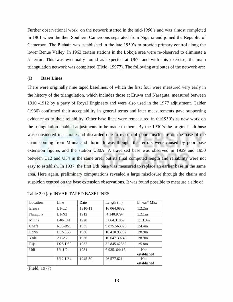
There were originally nine taped baselines, of which the first four were measured very early in
the history of the triangulation, which includes those at Eruwa and Naraguta, measured between
1910 -1912 by a party of Royal Engineers and were also used in the 1977 adjustment. Calder
(1936) confirmed their acceptability in general terms and later measurements gave supporting
evidence as to their reliability. Other base lines were remeasured in the1930‟s as new work on
the triangulation enabled adjustments to be made to them. By the 1930‟s the original Udi base
was considered inaccurate and discarded due to reason of poor misclosure on the base of the
chain coming from Minna and Ilorin. It was thought that errors were caused by poor base
extension figures and the station U80A. A traversed base was observed in 1939 and 1950
between U12 and U34 in the same area, but its final computed length and reliability were not
easy to establish. In 1937, the first Udi base was measured to replace an earlier base in the same
area. Here again, preliminary computations revealed a large misclosure through the chains and
suspicion centred on the base extension observations. It was found possible to measure a side of
Table 2.0 (a): INVAR TAPED BASELINES
Location Line Date Length (m) Linear* Misc.
Eruwa L1-L2 1910-11 16 064.6832 1:2.2m
Naraguta L1-N2 1912 4 148.9797 1:2.1m
Minna L40-L41 1928 5 664.31069 1:13.3m
Chafe R50-R51 1935 9 875.563023 1:4.4m
Ilorin L52-L53 1936 10 410.93092 1:8.9m
Yola A1-A2 1936 10 647.39748 1:8.9m
Rijau D28-D30 1937 32 845.42362 1:5.8m
Udi U1-U2 1931 6 935. 64416 Not
established
U12-U34 1945-50 26 577.621 Not
established
(Field, 1977)
14
the triangulation scheme with the aid of a subsidiary triangle at each end (Field, 1977). The
invar taped baselines data are shown in Table 2.0 (a).
(II) Astronomical Observations
Astronomical observations associated with the base line measurements were made, though not
necessarily completed at the same time for azimuth, but usually along one side of the base
extension figures close to the base itself. Longitudes were observed at three places. The use of
telegraph must have been adopted for the time check since the observations took place before the
1920‟s. Close, (1933) confirms this and quotes an accuracy of only 15” of arc.
Another azimuth observation was made between 1920 and 1930 before the 1st World War at
some of the oldest bases observed. The reason was presumably to eliminate some of the
misclosures which had emerged in the adjustment computations. The new azimuth line did not
always coincide with the old, for instance at Naraguta (Jos) the original azimuth was observed
along the baseline from N1 to N2 in 1912. By the time re-observation was thought necessary in
1928, the town of Jos had developed in the valley across which the base had been measured. The
new azimuth was then observed from N1 to N3, a station in the first base extension figure.
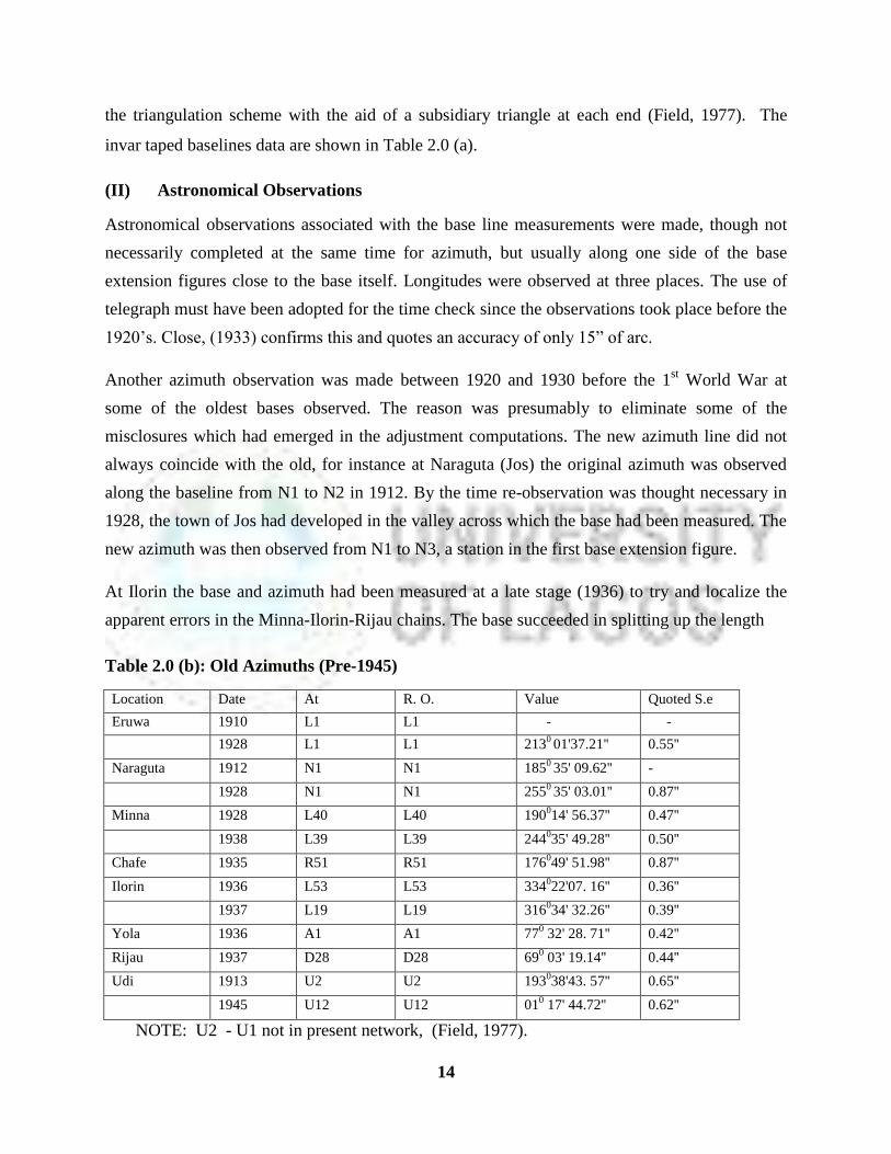
At Ilorin the base and azimuth had been measured at a late stage (1936) to try and localize the
apparent errors in the Minna-Ilorin-Rijau chains. The base succeeded in splitting up the length
Table 2.0 (b): Old Azimuths (Pre-1945)
Location Date At R. O. Value Quoted S.e
Eruwa 1910 L1 L1 - -
1928 L1 L1 2130 01'37.21'' 0.55''
Naraguta 1912 N1 N1 1850 35' 09.62'' -
1928 N1 N1 2550 35' 03.01'' 0.87''
Minna 1928 L40 L40 190014' 56.37'' 0.47''
1938 L39 L39 244035' 49.28'' 0.50''
Chafe 1935 R51 R51 176049' 51.98'' 0.87''
Ilorin 1936 L53 L53 334022'07. 16'' 0.36''
1937 L19 L19 316034' 32.26'' 0.39''
Yola 1936 A1 A1 770 32' 28. 71'' 0.42''
Rijau 1937 D28 D28 690 03' 19.14'' 0.44''
Udi 1913 U2 U2 193038'43. 57'' 0.65''
1945 U12 U12 010 17' 44.72'' 0.62''
NOTE: U2 - U1 not in present network, (Field, 1977).

15
error between Minna and Rijau, but large azimuth misclosures between Ilorin and the other base
figures were now found. In 1937, another azimuth was observed along an early line, the external
side of the Ilorin base which not L19-L21 to check the original azimuth. This confirmed the
earlier observations from L52-L53. The azimuth misclosures were eventually improved by
selecting angle observations in the Minna base extension net. The Table 2.0 (b) shows the
azimuths observed before 1945 (Field, 1977).
(III) The First Adjustment
The first adjustment was aborted by the second World War, and no further computation was
possible until the late 1950‟s when a review was made of the work done up to that time. This is
summarized by Cooper, (1974) and by Stamers and Sonola, (1955). As a result, angular re-
observations were made in the Lokoja area; D.O.S. was approached to do a completely new
adjustment of the network, and additional requirements of scale and orientation were specified
before such an adjustment could usefully be made.
(IV) Azimuth and Scale Check Programme:
Before the start of the Civil War, only 9 out of 20 Laplace stations and 16 out of 20 Scale check
triangles were completed, using Wild T4 theodolite, accurate timing piece, and Tellurometer
MRA2 and MRA3 instruments.
(V) Twelfth Parallel Survey
The Twelfth Parallel Survey was observed by the United States Corps of Engineers, with Federal
Surveys between 1967 and 1971 and covered a total of 81 points including Connections at 8
points to the Nigerian Primary Triangulation network, and 6 lower order stations.
(VI) Topocom Adjustment
In 1968, the so called Topocom Adjustment was done by the U.S Corps of Engineers, using data
available to them by then, an adjustment was made of most of the main triangulation network
stations. However details of the adjustment are not available.

16
(VII) Directorate of Overseas Survey
Two kinds of measurements done by the D.O.S are supplements to the primary network. They
are: (a) Tellurometer measurements of lengths of primary triangulation lines. (b) EDM traverses
running between stations of the primary chains.
(VIII) Primary Traverses in the South
Calder (1936) describes the measurement and procedure in some detail. Zeiss traverse equipment
and 500 foot steel tapes were used, and a linear misclosure of more than 1/60,000 was obtained.
These traverses were linked to the primary triangulation.
Table 2.0 (c): The Nigerian Triangulation Network
Chain Date No Mean Remarks
Observed Stations Side(Km)
Minna base net 1932 13 23.5
Karaguta base net 1932 11 8.1
Chafe base net 1935 8 23.8
Ilorin base net 1936 10 29.6
Yola base net 1936 6 12.4
Minna-Chafe (N) 1935 16 32.2
Naraguta-Chafe (N/K) 1929-35 56 18.4 Rearranged „37
Minna-Naraguta (N) 1933 23 40.4
Birnin Gwari-Naraguta (B) 1932 23 34.6
Kwongoma-Rijau (D) 1934-35 19 35.4
Rijau-Chafe ( R) 1935 44 36
Minna-Udi (L/U) 1930-37 45 34.8 Rearranged‟ 63
Ilorin-Eruwa (L) 1937 19 37.5
Ilorin-Rijau (D) 1934 33 42.6
Bauchi-Yola (A) 1933-36 42 36.2 Includes Yola bases net
Ropp,Yola (E) 1937 20 47.5
Udi-Cameroons (C ) 1945-54
1955-57
37 37.7
Lafia-Ogoja (U) 1945 14 45.5
Makurdi-Lokoja (P) 1957 16 45.4
Yola Nkambe (F) 1958-59 21 -
Nkambe-Takum (M) 1958-59 8 4.5 Part only of N chain
Biu. Madagali (C ) 1952-50 14 3.3
(Field, 1977).

17
The work was completed in 1939 and because of the vulnerable nature of traverses along the
main roads, many of the stations can no longer be recovered. A further series of primary
traverses, using EDM equipment, was established in the Niger Delta area by Shell B.P. These
connect to the primary triangulation near Idah (U97) and Arochukwu (C88). The summary of the
triangulation network is shown in Table 2.0 (c).
(IX) Controls used for Adjustment
The Controls used for the adjustment can be conveniently grouped into five categories:
1. The main triangulation network
2. The Twelfth parallel traverses
3. D.O.S. topographical traverses
4. The standard traverses
5. The EDM traverses by Shell B.P.
The configuration of the present Nigerian Horizontal Geodetic Network comprises of 515
stations. This includes all the 441 main triangulation network stations, the 39 stations of the
Twelfth Parallel Traverse and the 35 D.O.S. traverse stations.
In the Station numbering, each triangulation or traverse station bears a unique number, and is
also identified by the name of the hill feature on which it is established. The primary
triangulation points were originally numbered sequentially and prefixed by an initial letter
Provisional Coordinate Values: The observation (parametric) equation method of least squares
adjustment technique, used in the exercise, computes the corrections to be applied to a set of
provisional positional values for each station in the network. The result of the computation
generally were such that the input provisional values were sufficiently close to the final figures
so that no direction changes by more than one minute of arc, and no length changes by more than
1:400 exist (Bomford, 1971).
Provisional latitude and longitude were obtained for the stations in the networks from the
following sources:
Main Triangulation Network: For those stations included in the 1968 U.S. Topocom
adjustment, the final values were used as provisional coordinates. For certain stations not

18
included a provisional latitude and longitude were taken from either the 1930‟s first adjustment
or from the D.O.S. preliminary computations (M chain).
Twelfth Parallel Traverse: Final adjusted values for this traverse are shown in the 1977
adjustment by Field, (1977), including values for the eight points common with the Nigerian
triangulation network. As may be seen in Field, (1977), there is a difference of almost exactly 3”
are in latitude and longitude between origin of the survey. The final values have therefore been
corrected by 3” in arriving at the provisional coordinates for this adjustment.
D.O.S Traverse Stations : Approximate values for the 35 stations were supplied by D.O.S.
They have not been adjusted in sympathy with the triangulation, so cannot be expected to be as
precise as values for the other points. For this reason it can be anticipated that these set of
stations when incorporated would require several adjustment iterations before they are
acceptable.
(X) Spheroid, Origin and Unit of Length
Measurements are taken on the surface of the earth, which in this area lies between 0 and 2400
metres above the mean sea level (equipotential surface or geoid), (Field, 1977), a surface to
which all observations in the field are referred. The geoid is nearly spheroidal but is not exactly
regular in shape. For this reason, computations are made on a mathematical surface chosen to
approximate to the geoid shape in the Survey area. This surface is the ellipsoid of revolution
known as the spheroid.
Following Bomford (1971), there are eight independent constants to define in a spheroidal
reference system. They are:
1. The relation of the axis of revolution to the earth‟s
2. Mean polar axis.
3. Length of the major axis in the plane of the equator.
4. Relation of the lengths of the major and minor axis.
5. Latitude of survey origin.
6. Longitude of survey origin.
7. Spheroidal height at origin.

19
8. Reference longitude.
The Minor Axis of the Spheroid which lies along the polar axis of the earth varies in position in
relation to the body of the earth from year to year. The movement is in part periodic, due to
meteorological and dynamic causes, and in part constant. The total effect is a circular movement
about a mean pole of about 0.3” arc. Referring the movement to x and y axes along meridians 00
and 900 West, corrections can be made to convert astronomically observed values to the
Conventional International Origin (CIO) of 1930.
For observed azimuths the correction is - (x sin+ y cos ) cosφ (Field, 1977).
Lengths of the Major and Minor axes: The figure of the earth adopted in Nigeria, in common
with most other countries in Africa, South of the Sahara is the Clarke 1880 Spheroid. The
fundamental data are quoted by Calder (1936) and agree with MCCaw (1939) and Bomford
(1971)
a (semi – major axis) = 20 926 202 ft = 6 378 249.145m
f (flattening) = 1/293. 465
b (semi - minor axis) = a (1-f)
The conversion factor from international metres to geodetic feet is the Clarke foot legal meter
relation, (1 international meter = 3.2808 6933 geodetic feets).
Station L40, in Minna, is the origin of the Nigerian triangulation framework. The position of this
station is defined by Morley (1938) as:
Latitude 090 38 09”.000 N
Longitude 060 30‟ 59”.000 E
The height of L41 with reference to the mean sea level at Lagos is given by Calder (1936) as
follows:
Spirit Level height of L41 = 768.72ft.= 767.410 ft = 233.96 meters

20
The assumed latitude and longitude of L40 were obtained by combining values computed
through the triangulation network from astronomical observation stations in widely separated
areas. These are shown in Table 2.0 (d).
Table 2.0 (d): Coordinates of Minna Datum (L40) computed from astronomical
observation stations in widely separated areas.
Location Latitude Longitude
Enugu U12 90 38' 06.26'' -
Ilorin L53 - 60 30' 59.24''
Kaduna REW 1 90 38' 10.0'' 6
0 30' 54.4''
Kano K2 90 38' 08.8'' 6
0 30' 59.55''
Lagos Observatory 90 37' 58.95'' * 6
0 31' 0.6''
Lafia N26 90 38' 04.60'' 6
0 30' 56.9''
Minna L40 90 38' 11.7'' 6
0 30' 53.85'' **
Naraguta 90 38' 13.4'' 6
0 31' 0.5''
Olokomeji L3 90 38' 07.3'' 6
0 30' 57.65''
Onitsha U21 90 38' 07.36'' -
Zaria N144 90 38' 10.1'' 6
0 31' 0.95''
(Field, 1977).
* The latitude from Lagos Observatory was considered to be incorrect and hence omitted in
the computation of the origin values.
** It will be noticed there is an laplace correction (A-G) of –6E-15 x sin 90 38'' to the base
azimuth at Minna.
Reference Longitude is defined as the Greenwich Meridian.
(B) Typical network adjustment programmes already carried out around the world
These include the following:
(I) Los Angeles
Horizontal Geodetic Network measurements of six years of Global Positioning System (GPS)
data, 20 years of trilateration data and a century of triangulation, taped distance, and astronomic
azimuth measurements which were combined to provide the Horizontal Geodetic network of Los
Angeles (Land Information New Zealand, 2000).
21
(II) India
A huge amount of geodetic data and accurate maps on different scales exist. The Indian geodetic
control network is noted for its high precision in the world. The geodetic data, collected through
centuries of dedicated efforts, consists of the Great Trignometrical (G.T.) Triangulation Network
of India, the Satellite Survey Control Network, the High Precision, Precision and Secondary
Levelling Network, the Laplace Stations Network, the Gravity Stations Network, the Tidal
Stations Network and the Geomagnetic Stations Network. The topographical maps by
Government of India are another such database. A wealth of information is contained in this
databank.
(III) Korean peninsula
The first Nationwide Geodetic Network in the Korean peninsula was established in 1910-1915
by the Bureau of Land Survey. The Government-General of Korea in cooperation with the
Japanese Military Land Survey. The major network of the old triangulation consisted of thirteen
baselines, primary and secondary networks, and were connected to the Tokyo Datum with the
triangulation through Tsushima Islands. After the World War II, the network over the Korean
(Tsushima straight) was resurveyed in 1954 by US Army Map Service Far East in cooperation
with Geographical Survey Institute of Japan, in order to strengthen the connection between
Korea and Japan.
To keep consistency with the old coordinates system, the Primary Precise Geodetic Network
(PPGN) was adjusted in the way that its official coordinates are same as the old ones.
Unfortunately, original records of the old survey were lost during the Korean War, and we only
have a set of coordinates of triangulation points now.
The establishment of PPGN was carried out in 1975-1994 by National Geography Institute of
Korea. The PPGN consists of 1155 points including 175 (~15 %) old first- and second-order
triangulation points (normal points) not damaged by the war, and its mean side-length is about 11
km. The coordinates of PPGN derived in 1995 have been held fixed since. During the 1980's and
1990's the increased use of satellite based geodetic measuring systems - such as the GPS - began
to impact on the utility of the national geodetic datum in Korea. Under this impact, new
geocentric datum, new Korean Geodetic Datum 2000 (KGD2000), designed and built during

22
1998, is realized through ITRF97 and used the GRS80 ellipsoid (Choi, 1998: Grant, Blick,
Pearse, Beavan and Morgan, 1999; Stephen, Sever, Bertiger, Heflin, Hurst, Muellerschoen, Wu,
Yunk, 1996).
(IV) Great Britain
In Great Britain Geodetic Network, three coordinate systems are considered:The National GPS
Network, a modern 3-D TRF using the ETRS89 datum. This coordinate system is the basis of
modern Ordnance Survey control survey (the surveyor's jargon for adding local points to a TRF
for mapping purposes), and will become the basis of definition of all Ordnance Survey
coordinates over the next few years. A subset of the Active Layer of the National GPS Network
has been ratified as the official densification of ETRF89 in Great Britain.
The National Grid, a traditional horizontal coordinate system, which consists of: a traditional
geodetic datum using the Airy ellipsoid; a TRF called OSGB36® (Ordnance Survey Great Britain
1936) which was observed by theodolite triangulation of trig pillars; and a Transverse Mercator
map projection, allowing the use of easting and northing coordinates. This coordinate system is
important because it is used to describe the horizontal positions of features on British maps.
However, its historical origins and observation methods are not of interest to most users.
National Grid coordinates are these days determined by GPS rather than theodolite triangulation.
Ordinance Datum Newlyn (ODN), a 'traditional' vertical coordinate system, consisting of a tide
gauge datum with initial point at Newlyn (Cornwall) and a TRF observed by spirit levelling
between 200 fundamental bench marks (FBMs) across Britain. The TRF is densified by more
than half a million lower-accuracy bench marks. Each bench mark has an orthometric height (not
ellipsoid height or accurate horizontal position). This coordinate system is important because it is
used to describe vertical positions of features on British maps (for example, spot heights and
contours) in terms of height above mean sea level. Again, its historical origins and observation
methods are not of interest to most users. The word Datum in the title refers strictly speaking, to
the tide gauge initial point only, not to the national TRF of levelled bench marks.
The National GPS Network provides a single 3-D TRF which unifies ODN and OSGB36 via
transformation software Using transformation techniques, precise positions can be determined
by GPS in ETRS89 using the National GPS Network and then converted to National Grid and
23
ODN coordinates. This is the approach used today by Ordnance Survey (Paul and Jackson, 1999;
Land Information New Zealand, 2000).
(V) Uganda
The Uganda Triangulation Network was established by the British colonial administration in the
20th
century. This was done in Phases, starting with the primary, followed by the secondary and
finally the tertiary network. A total of 1730 stations were established throughout the country. The
computation of the network was based on the Clark 1858 ellipsoid and the curvilinear horizontal
positions were projected onto the UTM projection which was used to map the country. Later, the
re- computation of the country‟s network was based on Clark 1880 modified ellipsoid. There is a
program in place to re-observe the existing network and other new points with GPS satellite
method (Rainsford, 1948; Okia and Kitaka, 2000).
(VI) Kenya
In Kenya, the Directorate of overseas surveys began the establishment of the primary, secondary
and tertiary triangulation and traverse networks around 1950. The mapping of the country was
also done by them until they departed from the country in 1983. The reference ellipsoid and the
projection used for mapping the country are Clark 1880 and UTM respectively (Kenya Institute
of Surveying and mapping Nairobi, 2000).
(VII) Egyptian
The existing Egyptian geodetic network, which dates back to the first decade of the twentieth
century, has been studied and adjusted in two and three-dimensions by several researchers.
All previous trials showed that there is a problem of some kind of distortion due to the inaccurate
adjustment and lack of geoidal information. GPS is used extensively in the last decade. The first
order geodetic horizontal control network of Egypt contains two main networks, Network (1) and
Network (2), [Cole, 1944] and these networks were extended to other African nations. The
networks comprise 402 stations and were established between 1907 and 1968 (Saad and Elsayed,
2007).
(C) Survey Requirement
Like any other field of study, most especially in Geodesy, the need and importance of the
bearable limit of any process is an essential consideration in the design, construction and
24
measuring stages in order to meet some given specifications. Surveying constitutes a unique
field where this consideration operates with much emphasis laid on the accuracy achievable in a
given process such as Geodetic Networks. The various practical requirements for accuracy can
be attained with the minimum effort and time through a suitable choice of most appropriate
instrument and an efficient and cost saving measuring procedure.
Observational precision in contemporary surveying practice is characterized by the standard
deviation or variance of individual observations. In order that useful statistical propagation of
this error can occur, these variances (variance covariance) are assumed to have a multivariate
normal distribution with vector of zero mean. This implies that the variances must be composed
of random errors and that any error or inaccuracy which is systematic in nature has already been
accounted for and removed, either by solving for the systematic component through an
adjustment process, eliminating it through appropriate observation procedures, or eliminating it
by other empirical techniques.
The determination of the geodetic coordinates of points on the ellipsoid can be expressed as
Direct and Indirect Problems (Ashkenazi, 1967 and 1970). The least squares method of
observation equation which take into consideration the curvilinear shape of the earth expresses
the adjusted observation such as angles, distances, azimuths as a function of the unknown
stations coordinates (Bomford, 1971 and Ashkenazi, 1972).
Ayeni (1980, 2002 and 2003) and Ayeni, et. al, (2005) from their work – “Determination of the
most appropriate least squares method for position determination in a triangulation
network” at an International workshop on Geodesy & Geodynamics, in Toro, Bauchi State of
Nigeria showed that, of the four mathematical techniques (simultaneous; sequential; phase and
combined) used in a sample geodetic adjustment, the simultaneous technique yielded the best
suitability criteria in terms of network standard deviation, trace of the variance covariance matrix
of the adjusted parameters and observations, and least time of computation.
(D) Application of Optimization Technique to Triangulation network
Of the three successful optimization algorithms (Simulated Annealing (SA); Genetic
Algorithms (GA); and Gaussian adaptation (NA);) used in geodetic network problem, Goldberg,
(1989 and 2002), Berne and Baselga (2003) and Donald (1970) confirmed that the simulated
annealing gave the best suitability criteria because it seeks the lowest energy state of geodetic
coordinates (stable state or final adjusted coordinates of station) of individual stations instead of

25
the maximum fitness of the network. Other benefits are less time of computation, lower cost, less
storage, high reliability for global solution. The Simulated Annealing was used for the First-
order design of sample geodetic networks by Berne and Baselga (2003).
Ayeni, et.al, (2006) in their work on “Application of Optimization Technique (Simulated
Annealing Method) to Triangulation network.” showed better suitability criteria for the method
of Simulated Annealing over the Simultaneous method in terms of network standard deviation,
trace of the variance covariance matrix of the adjusted parameters and observations, and high
reliability for global solution because it seeks the lowest energy state of geodetic coordinates of
individual stations instead of the maximum fitness of the network. Beside the additional
optimization algorithm in the SA, it incorporate simultaneous iterative scheme which ensures a
holistic adjustment of the network.
(E) Application of Global Navigation Satellite Systems (GNSS)
At present the Global Navigation Satellite Systems (GNSS) are used for geodetic work. GNSS is
the standard generic term for satellite navigation systems ("sat nav"). It provide autonomous geo-
spatial positioning with global coverage. It allows small electronic receivers to determine their
location (longitude, latitude, altitude) to within a few meters using time signals transmitted
along a line of sight by radio from satellites. Receivers calculate the precise time as well as
position, which can be used as a reference for scientific experiments.
As at the year 2010, the United States Navstar Global Positioning System (GPS) is the only fully
operational system. Today, the Russian Glonass (GNSS) and its in the process of being restored
to full operation (21 of 24 satellites are operational). The European Union‟s Galileo Positioning
System is a GNSS in initial deployment phase, scheduled to be operational in 2014. The People‟s
Republic of China has indicated it will expand its regional Beidou navigational system into the
global Compass navigation system by 2020.
The global coverage for each system is generally achieved by a constellation of 20–30 Medium
Earth Orbit (MEO) satellites spread between several orbital planes. The actual systems vary, but
use orbit inclinations of >50° and orbital periods of roughly twelve hours (height 20,000 km /
12,500 miles). Table 2.0 (e) shows the comparison of GNSS systems.

26
Table 2.0 (e):Comparison of GNSS Systems
System Country Coding Orbital height & period
Number of satellites Frequency Status
GPS United States CDMA 20,200km,
12.0h ≥ 24
1.57542 GHz (L1 signal) 1.2276 GHz (L2 signal)
operational
GLONASS Russia FDMA/CDMA 19,100km, 11.3h
24 (30 when CDMA signal launches)
Around 1.602 GHz (SP) Around 1.246 GHz (SP)
operational with restrictions, CDMA in preparation
Galileo European Union CDMA 23,222km,
14.1h
2 test bed satellites in orbit 22 operational satellites budgeted
1.164-1.215 GHz (E5a and E5b) 1.215-1.300 GHz (E6) 1.559-1.592 GHz (E2-L1-E11)
in preparation
COMPASS China CDMA 21,150km, 12.6h 35
[5]
B1: 1,561098 Ghz B1-2: 1.589742 Ghz B2: 1.207.14 Ghz B3: 1.26852 Ghz
5 satellites operational, additional 30 satellites planned
(Wikipedia, 2010).
2.1 THEORETICAL FRAMEWORK
Generally the methods for the adjustment of Geodetic networks are based on the following
considerations:
(i) Computations of geodetic coordinates on the ellipsoid.
(ii) The observation equations on the ellipsoid.
(iii) Least Squares method.
(iv) Error ellipse equations.
(v) Federal Geodetic Control Committee (FGCC) standards and specifications.
(vi) Optimization technique suitability for large geodetic network.
2.1.1 COMPUTATIONS OF GEODETIC COORDINATES ON THE ELLIPSOID.
The problems of the geodetic coordinates of points on the ellipsoid can be expressed as Direct
and Indirect Problems, (Ashkenazi, 1967 and 1970).
27
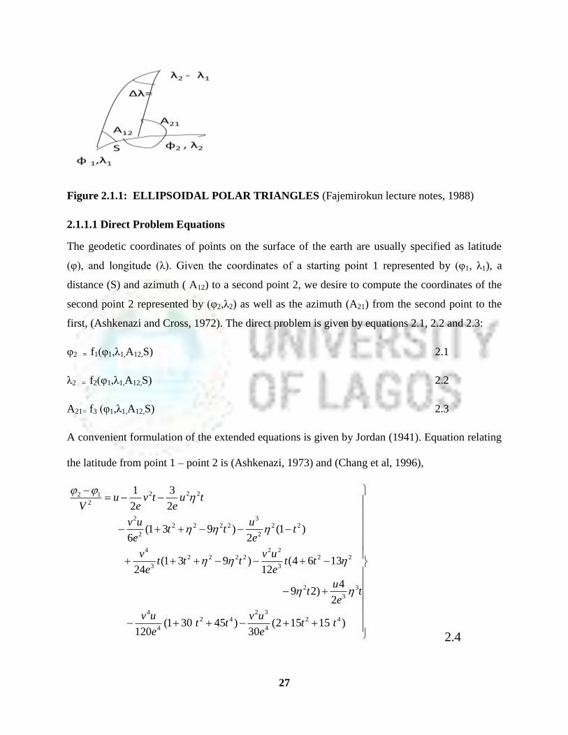
Figure 2.1.1: ELLIPSOIDAL POLAR TRIANGLES (Fajemirokun lecture notes, 1988)
2.1.1.1 Direct Problem Equations
The geodetic coordinates of points on the surface of the earth are usually specified as latitude
(φ), and longitude (λ). Given the coordinates of a starting point 1 represented by (φ1, λ1), a
distance (S) and azimuth ( A12) to a second point 2, we desire to compute the coordinates of the
second point 2 represented by (φ2,λ2) as well as the azimuth (A21) from the second point to the
first, (Ashkenazi and Cross, 1972). The direct problem is given by equations 2.1, 2.2 and 2.3:
φ2 = f1(φ1,λ1,A12,S) 2.1
λ2 = f2(φ1,λ1,A12,S) 2.2
A21= f3 (φ1,λ1,A12,S) 2.3
A convenient formulation of the extended equations is given by Jordan (1941). Equation relating
the latitude from point 1 – point 2 is (Ashkenazi, 1973) and (Chang et al, 1996),
2.4
)15152(30
)45301(120
2
4)29
1364(12
)931(24
)1(2
)931(6
2
3
2
1
42
4
3242
4
4
3
3
2
22
3
222222
3
4
22
2
32222
2
2
222
2
12
tte
uvtt
e
uv
te
ut
tte
uvttt
e
v
te
utt
e
uv
tue
tve
uV

27
Equation relating the Longitudes from point 1 to point 2
2.5
Equation relating the forward azimuth and backward azimuth between points 1 and point 2
2.6
where in our notation:
2.7
where
t = λ2 – λ1 2.8
)30201(15
)15152(15
)31(15
)32(3
)31(3
)31(33
1cos) - (
42
4
2342
4
422
4
5
22
3
332
3
3
22
2
22
2
3
12
tte
uvtt
e
vutt
e
v
tte
vutt
e
uv
te
vut
e
v
vute
v
)12018061(120
)24028058(120
)24201(120
)8624
285(24
)8224201(24
)465(6
)21(6
)21(2
'
42
4
23
42
4
2342
4
5
2224
2
3
322242
3
3
422
2
222
2
3
22
ttte
uv
ttte
uvttt
e
v
tt
te
vuttt
e
uv
tte
vutt
e
v
te
vuvt
28
a= length of semi major axis
b=length of semi minor axis
e = 1st eccentricity
e' = 2nd
eccentricity
For angular units in radians set to 1. Bagratuni (1962 and 1967) indicated accuracy up to
130km; While Grushinsky (1963) indicated accuracy up to 600-800km.
2.1.1.2 Indirect Problem (Inverse Solution)
The indirect problem can be expressed as shown in equations 2.14, 2.15 and 2.16
Given the coordinates of the end points of the line, we desire to find the azimuths ( A12), (A21)
and distance S.
S = f4(φ1,λ1, φ2 , λ2) 2.14
A12 = f5(φ1,λ1, φ2 , λ2) 2.15
A21= f6 (φ1,λ1, φ2 , λ2) 2.16
The solution of the inverse problem can be solved using series expansions and it is done through
an iterative procedure, (Baarda, 1977), (Bannister and Raymond, 1975)
29
where A and B are functions of s, A12, and 1. We now solve equations 2.17 and 2.18 assuming
A and B are known, (Bradley, 1939 and Butler, 1966).
Letting =2- 1 and = 2 - 1
We have:
V12=1+1
2 ` 2.21a
12=e‟
2cos
21 2.21b
Dividing equation (2.19) by equation (2.20) and rearranging terms:
[
] 22
In addition S can be found from either of the equations (2.17 and 2.18) as
Knowing , , and 1, and setting A and B to zero as a first approximation to the azimuth
(A12(1)
) in equation (2.22), we have from equation (2.17 and 2.18), (Bomford, 1971 and
Richard, 1980):
[
]
Setting A equal to zero in equation (2.23), and using the azimuth from (2.24) we compute the
first approximation to the distance as:

30
Using the now known values of A(t)
12 and S(1)
we can compute values for A and B which can
then be used in equations (2.17) and (2.18) to find better values for A12 and S. The process is
iterated until the values of A12 and S do not change beyond a specified amount (Stamers and
Sonola, 1955; U.S. Department of Commerce, 1935; and Gazdzicki, 1976).
In this study both the direct method and indirect methods are used in the adjustment.
2.1.2 THE OBSERVATION EQUATIONS ON THE ELLIPSOID
These are equations used in geodetic adjustment which take into consideration the curvilinear
shape of the earth. Bomford (1971) and Ashkenazi (1972) gave equivalent formula linking dA12,
dφ, dλ, and dD where the first three are in seconds of arc, the last is in linear units as defined
below:
Ai j is azimuth of geodesic from i to j;
Di j is length of geodesic from i to j;
φi is provisional latitude of station I
λi is provisional longitude of station I
pi is meridional radius of curvature of spheroid at i
vi radius of curvature at right angles to meridian at i
The Figure 2.1.2 is a sample of triangulation net with nodes/station I, J and K.

31
The following defined terms (equations 2.26 – 2.33) can computed for the angular, distance and
azimuth observation equations for the network (equations 2.36 – 2.38).
From these basic equations, observations equations may be formed, and grouped into a series of
simultaneous linear equations dAij and dDij are the small changes in the observations needed to
convert from observed (O) to computed (C) values) (Bomford, 1971 and Richard, 1980).
Thus
Vij in equations (2.36 – 2.38) is the small correction to the observed value in the solution. The
observed values in this network are of three kinds, clockwise angles at pont j indicated by i j k,
distance i j, and Laplace azimuths i j.
The three types of observation equation according to Bomford (1971) and Ashkenazi (1972)
are:

32
(i) Clockwise angles i j k
(Ki k –Ki j) dφ i + (Li k – Li j) dλi – Mi j dφ j – Ni j dλj + Mi k dφ k + Ni k dλk =
(O – C)i j k + Vi j k 2.36
where: (O – C) i j k is the small difference in seconds between observed (O) and computed (C)
angles; Vi j k is the correction to the observed angle.
(ii) Distance i j
Pi j dφ i + Qi j dλi + Ri j dφ j + Si j dλi = (O – C)i j + Vi 2.37
(O – C) is in linear units.
(iii) Laplace azimuths
Ki j dφ i + (Li j – sinφ i) dλi + Mi j dφ j + Ni j dλj = (O – C)i j + Vi j 2.38
(Bomford, 1971 and Richard, 1980)
In this equation the expression (Li j – sinφ i) allows for the Laplace correction (LA – LG) sinφ i
which changes the geodetic azimuth of the line in accordance with the deviation of the vertical at
the point of observation. Successive approximations to the correct geodetic azimuth are thus not
necessary (Even-Tzur and Papo, 1996; Even-Tzur, 2001; Grant, Blick, Pearse, Beavan and
Morgan, 1999).
2.1.3 LEAST SQUARES MATHEMATICAL METHOD:
It is generally accepted that the precision of a measurement may be improved by increasing the
number of observations. The redundant observations arising therefore, however creates a number
of problems. For example discrepancies may occur between repeated observations since each
observation has a certain amount of insecurity (precision) attached to it. Such discrepancies
therefore have to be reconciled (adjusted) so as to obtain the most satisfactory (most probable or
adjusted) values of unknown quantities. Also, redundant observations may lead to redundant but
consistent equations in which there are more equations than unknown quantities. There is
therefore the need to obtain not only the most probable values of unknown quantities but also to
find a unique solution for these quantities.

33
The method of least squares is a method which makes use of redundant observations in the
mathematical modeling of a given problem with a view to minimizing the sum of the squares of
discrepancies (residuals) between the observations and their most probable (adjusted ) values
subject to the prevailing mathematical model.
There are two types of models used in least square problems, (Ayeni, 2002 & 2003).
(i) Condition equation, which can be expressed as:
where is the adjusted observable, e.g. angles and distances
(ii) Observation Equation, which can be expressed as:
where: is the adjusted parameter.
In this study, we wish to determine the parameter ( , hence equation 2.40 shall be considered.
There are four common mathematical techniques used in the least squares observation equations
method, (Ayeni, 1980, 2002 and 2003 and Cross, 1974). They are:
2.1.3.1 Simultaneous Method.
Observation Equation method of Simultaneous approach is shown in Figure 2.1.3a and given by
equation (2.40). Each of the network triangle observations are combined in a single process of
adjustment to achieve a unique and best estimate values of the network stations coordinates.
Linearised form is given by equation (2.41)
( )
V= Ax + L 2.41a
where La = L
b + V,
Lb = Vector of observation,

34
Xª = adjusted parameters
V = the vector of residuals,
X = the solution vectors,
x = the correction vector = Xa - X
o
Xº = the approximate parameters,
The resulting normal equation is shown in equation (2.42)
Figure 2.1.3a: SIMULTANEOUS METHOD

35
P = weight matrix design as the inverse of the square of the standard error of observations.
Iterative solution is necessary to compensate for linearization in equation (2.41) giving rise to
equation - (2.43)
Xª (i+1) = X1º + xi 2.43
At convergence 2.43a
where i represent the ith
iteration
2.1.3.2 Sequential Method.
Observation Equation method which is used for Sequential approach is shown in Figure (2.1.3b)
and defined by equation (2.44) and (2.45) (Ayeni, 2001). This method allows the effect of
additional observations and new parameters on observation equation model of a previously
adjusted observation and parameter (coordinates) of some triangles within the network. Hence
triangles in Figure 2.1.3b are chosen on sequential bases to allow for the addition of a new
triangle observation and parameter in any subsequent adjustment.
V = the vector of residuals,
X = the solution vectors,
x = the correction vectors,
Xº = the approximate parameters,
The resulting normal equation is shown in equation (2.42)
V1 = A1x + L1 2.46
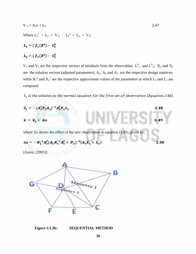
36
V 2 = A2x + L2 2.47
Where L1a = L1 + V1; L2
a = L2 + V2;
V1 and V2 are the respective vectors of residuals from the observables Lb
1 and Lb
2; X1 and X2
are the solution vectors (adjusted parameters); A1, A2 and A3 are the respective design matrices;
while X1o and X2
o are the respective approximate values of the parameters at which L1 and L2 are
computed.
where Δx shows the effect of the new observation in equation (2,45), given by:
(Ayeni, (2001))
Figure 2.1.3b: SEQUENTIAL METHOD

37
where ∆X is the effect of the additional observation and new parameters on observation equation
model. Iterative solution is necessary to compensate for linearization
where i represent ith iteration which converges as xi = 0 and Xai+1 is the final adjusted
parameters (coordinates) of the network stations.
N1= A1TP1A1
N2 =A2TP2A2
U1 = A1TP1L1
U2 = A2TP2L2
Xa1 and X
a2 are adjusted parameters; L
a1 and L
a2 are adjusted observations;
L1 = 1(Xo1) – L
b 1,
L2 = 2(Xo1) – L
b 2
V1 and V2 are the vectors of residuals; X1 and X2 are the solution vectors; A1 and A2 are the
respective design matrices; X1o and are the approximate values of the parameters.
P2 = weight matrix of L2
2.1.3.3: Phase Method.
Observation Equation method which is used for Phase approach is shown in Figure (2.1.3c) and
defined by equations (2.52) and (2.53), (Ayeni, 1985 and 2003), (Biacs, Krakiwsky and
Lapucha, 1990). This method allows the network triangle observation and parameter to be
38
adjusted in phases. Adjoining phases incorporates any result of previously adjusted parameter
reappearing in it for subsequent adjustment.
La1 = f1 (X
a1) 2.52
La2 = f2 (X
a2) 2.53
The constraint model from equation (2.52) after adjustment of the first phase is:
and their linearized forms are given by equations (2.54, 2.55 and 2.55a)
V1 = A1x1 + L1 2.54
V2 = A2x2 + L2 2.55
Vx = x1 + L3 2.55a
Note that the adjusted parameters in the first Phase, equation (2.52) are used as approximate
values in the second Phase, equation (2.53).
where La1 = L1 + V1,
La2 = L2 + V2
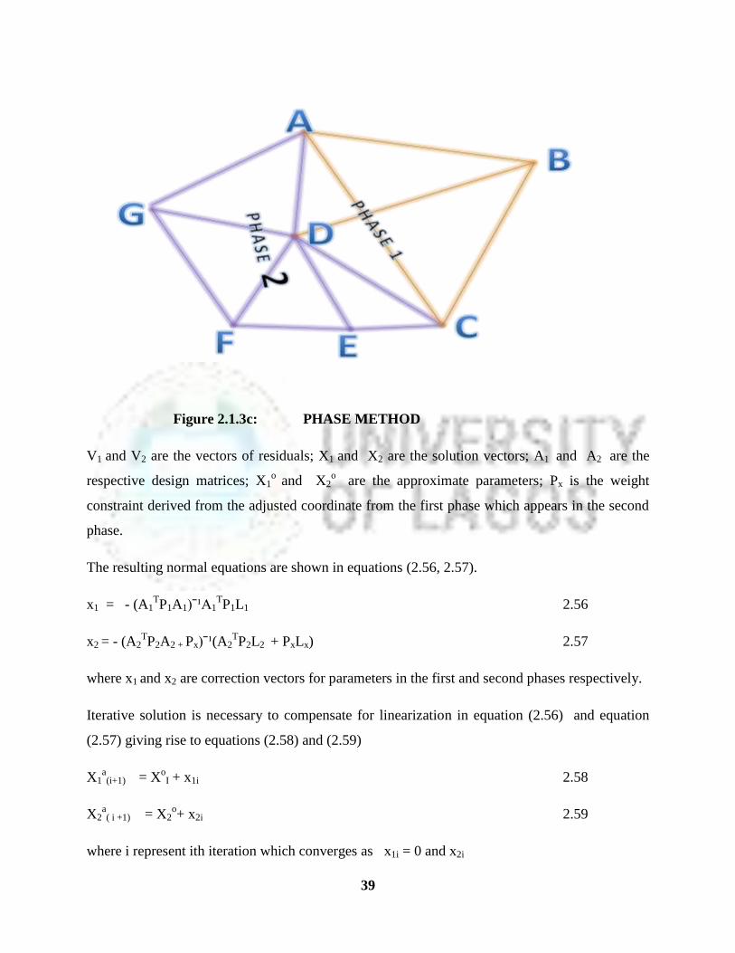
39
Figure 2.1.3c: PHASE METHOD
V1 and V2 are the vectors of residuals; X1 and X2 are the solution vectors; A1 and A2 are the
respective design matrices; X1o and X2
o are the approximate parameters; Px is the weight
constraint derived from the adjusted coordinate from the first phase which appears in the second
phase.
The resulting normal equations are shown in equations (2.56, 2.57).
x1 = - (A1TP1A1)ˉ¹A1
TP1L1 2.56
x2 = - (A2TP2A2 + Px)ˉ¹(A2
TP2L2 + PxLx) 2.57
where x1 and x2 are correction vectors for parameters in the first and second phases respectively.
Iterative solution is necessary to compensate for linearization in equation (2.56) and equation
(2.57) giving rise to equations (2.58) and (2.59)
X1a(i+1) = X
oI + x1i 2.58
X2a( i +1) = X2
o+ x2i 2.59
where i represent ith iteration which converges as x1i = 0 and x2i
40
2.1.3.4 Combined (Phase & Sequential) Method.
Observation Equation method which is used for Combined approach is shown in Figure (2.3d)
and defined by equations (2.60) and (2.61), (Ayeni, 2001 and 2003; Cooper, 1974; and Cross,
1974). Here the network triangles are adjusted sequentially in phases. Additional phases
observation and parameter are added to all the result of the previous adjustment, sequentially.
La1 = 1 (X
a1) 2.60
La2 = 2 (X
a1, X
a2) 2.61
STEP 1
The equations (2.60 and 2.61) can be considered for phase adjustment, in which case equation
(2.60) is adjusted first to obtain:
x*1 = - (A1TPA1)ˉ¹ A1
TPL1 2.62
Using X1* as observations in the adjustment of equation (2.60) along with weight matrix QX1
QX1 = - (A1TPA1 )ˉ¹
STEP 2
LaX1 = X
a1 2.63
La2 = 2 (X
a1, X
a2) 2.64
Linearising equation (2.63) and (2.64)
Vx1 = x1 + Lx1 2.65
V2= A2x1 + A3x2 + L2 2.66
where Lax1 = Lx1 + Vx1

41
Figure 2.1.3d : COMBINED METHOD
La2 = L2 + V2
Vx1 & V2 are the vectors of residuals; x1 and x2 are the correction vectors of the parameters; A1,
A2 & A3 are the respective design matrices; X1o and X2
o are the approximate parameters.
The resulting normal equations are shown in the equations below:
X1= x1* - Pˉ¹x1A2TK2 2.67
X2 = (A3T(A2Pˉ
¹X1A2
T+Pˉ
¹2)ˉ
¹A3
T(A2Pˉ
¹X1A2
T+Pˉ
¹2 )ˉ¹(A2x1* +L2) 2.68
Where
K2 = (A2 Pˉ¹X1 A2
T+Pˉ
¹2)ˉ
¹(A2X2+A2x1* +L2)
PX1 = σ2
o Σˉ¹Χª1

42
X1 = Xª1
L2 = Lº2 – L2
Lº2 = 2(Xº1 ,Xº2 )
Xª2 = Xº2 + X2
P2 = weight matrix of L2;
Iterative solution is necessary to compensate for linearization in equations (2.59) and (2.63)
giving rise to equation - (2.66), (2.67 and 2.68).
Xª1( i+1) = XºI + XI 2.69
Xª2 (i+1) = Xº 2 + X2 2.70
Where i represent ith iteration which converges as: XI = 0 & X2 = 0
2.1.4 NETWORK GEOMETRY ASSESSMENT
The least squares estimate of the adjusted parameters Xa is given for the linear case by equation
(2.71):
X = N -1
U 2.71
Where N = ATPA; U = A
TPL
b;
N is called normal coefficient matrix.
The unbiased estimate of the covariance matrix of adjusted parameters is given by equation
(3.21) as:
(
)
N-1
= weight coefficient matrix and denoted by Q i.e Q = N-1
.
Where ∑x is an error matrix since standard errors associated with the adjusted parameters may be
estimated from its diagonal elements.

43
The covariance matrix for the unknown parameter before adjustment is given as equation (3.1)
as:
Where: σ²o is the a-priori variance of unit weight of the observations and P is the weights of the
observations.
The details of these equations are discussed under methodology in chapter three.
2.1.5 FEDERAL GEODETIC CONTROL COMMITTEE (FGCC) STANDARDS AND
SPECIFICATIONS.
FGCC is a committee set up by world survey body to control: Specifications to Support
Classification; Standards of Accuracy; and General Specifications of Geodetic Control Surveys;
The Nigerian Institution of Surveyors standards and specifications (NIS, 2008) also agrees with
(FGCC, 2006). These are necessary due to the rapid changes in the requirements and methods for
acquisition of geodetic control (Hotline, 1935; Holland, 1975; Ingham, 1975; Hongsic Yun
2001).
2.1.5.1 Standards
The classification standards of the National Geodetic Control Networks are based on accuracy.
This means that when control points in a particular survey are classified, they are certified as
having datum values consistent with all other points in the network, not merely those within that
particular survey. It is not observation closures within a survey which are used to classify control
points, but the ability of that survey to duplicate already established control values. This
comparison takes into account models of crustal motion, refraction and any other systematic
effects known to influence the survey measurements (Baarda, 1977).
A variance factor ratio for the new survey combined with network data is computed by the
Iterated Almost Unbiased Estimator (IAUE) method and (FGCC, 2006). If the variance factor
ratio is reasonably close to 1.0 (typically less than 1.5), then the survey is considered to check
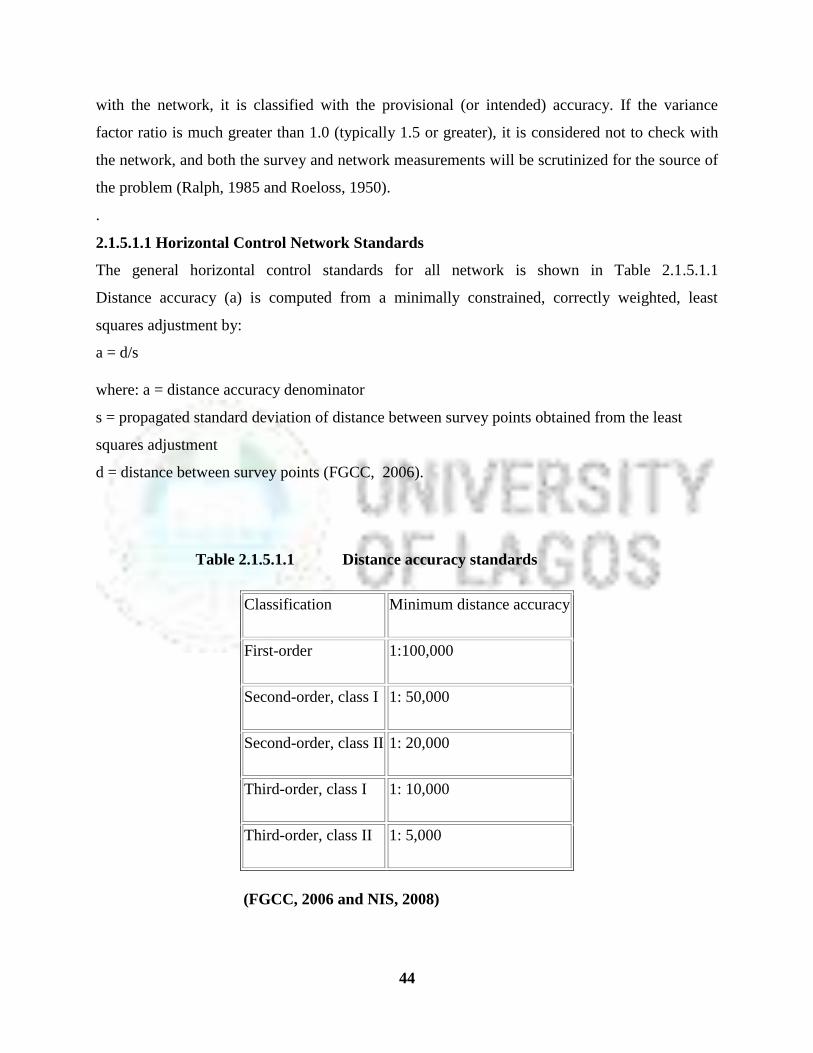
44
with the network, it is classified with the provisional (or intended) accuracy. If the variance
factor ratio is much greater than 1.0 (typically 1.5 or greater), it is considered not to check with
the network, and both the survey and network measurements will be scrutinized for the source of
the problem (Ralph, 1985 and Roeloss, 1950).
.
2.1.5.1.1 Horizontal Control Network Standards
The general horizontal control standards for all network is shown in Table 2.1.5.1.1
Distance accuracy (a) is computed from a minimally constrained, correctly weighted, least
squares adjustment by:
a = d/s
where: a = distance accuracy denominator
s = propagated standard deviation of distance between survey points obtained from the least
squares adjustment
d = distance between survey points (FGCC, 2006).
Table 2.1.5.1.1 Distance accuracy standards
Classification Minimum distance accuracy
First-order 1:100,000
Second-order, class I 1: 50,000
Second-order, class II 1: 20,000
Third-order, class I 1: 10,000
Third-order, class II 1: 5,000
(FGCC, 2006 and NIS, 2008)
45
2.1.5.1.2 Monumentation
Control points should be part of the National Geodetic Horizontal Network only if they possess
permanence, horizontal stability with respect to the Earth's crust and a horizontal location which
can be defined as a point. First-order and second-order class I control points should have an
underground mark, at least two monumental reference marks at right angles to one another, and
at least one monumental azimuth mark no less than 400 m from the control point. Replacement
of a temporary mark by a more permanent mark is not acceptable unless the two marks are
connected in timely fashion by survey observations of sufficient accuracy (FGCC, 2006).
2.1.5.2 Specifications
All measurement systems regardless of their nature have certain common qualities. The
measurement system specifications follow a prescribed structure as outlined in Section 2.1.5.2.1.
These specifications describe the important components and state permissible tolerances used in
a general context of accurate surveying methods. The user is cautioned that these specifications
are not substitutes for manuals that detail recommended field operations and procedures
(McCaw, 1935; Morley, 1938; Munsey, 1949; Lindlohr, and. Wells 1985; Atilola, 1985 and
1986; Omogunloye, 1988 and 1990; and FGCC, 2006).
2.1.5.2.1 Triangulation
Triangulation is a control establishment system comprising of joined or overlapping triangles of
angular observations supported by occasional distance and astronomic observations (at Laplace
Stations). Triangulation can also be used to extend horizontal control (Richardus, 1966; Ralph,
1985; and FGCC, 2006). The Network geometry (Table 2.1.5.1.2) shows the configuration
usually used in the specifying of different orders and classes of network.
The new survey is required to tie to at least four well spaced network control points. These
Network points must have datum values equivalent to or better than the intended order and class
of the new survey. For example, in an arc of triangulation, at least two network control points
should be occupied at each end of the arc. Whenever the distance between two new unconnected
survey points is less than 20 percent of the distance between those points traced along existing or
new connections, a direct connection should be made between those two survey points. In
addition, the survey should tie into any sufficiently accurate network control points within the
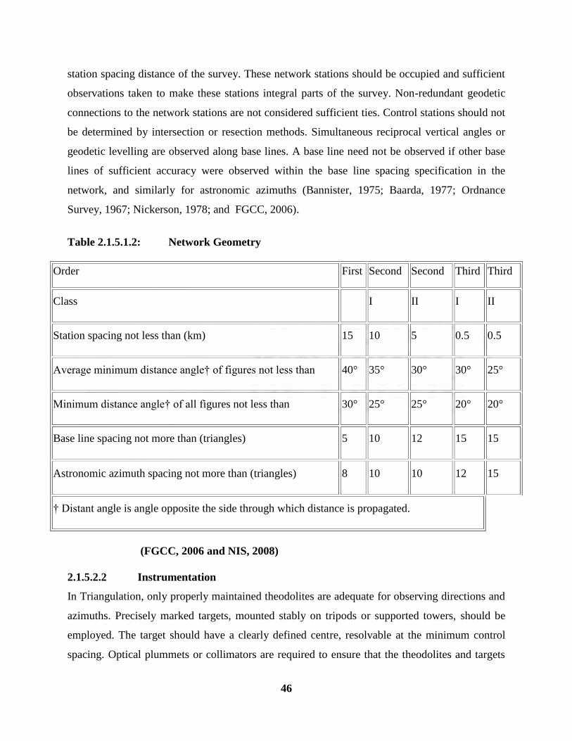
46
station spacing distance of the survey. These network stations should be occupied and sufficient
observations taken to make these stations integral parts of the survey. Non-redundant geodetic
connections to the network stations are not considered sufficient ties. Control stations should not
be determined by intersection or resection methods. Simultaneous reciprocal vertical angles or
geodetic levelling are observed along base lines. A base line need not be observed if other base
lines of sufficient accuracy were observed within the base line spacing specification in the
network, and similarly for astronomic azimuths (Bannister, 1975; Baarda, 1977; Ordnance
Survey, 1967; Nickerson, 1978; and FGCC, 2006).
Table 2.1.5.1.2: Network Geometry
Order First Second Second Third Third
Class I II I II
Station spacing not less than (km) 15 10 5 0.5 0.5
Average minimum distance angle† of figures not less than 40° 35° 30° 30° 25°
Minimum distance angle† of all figures not less than 30° 25° 25° 20° 20°
Base line spacing not more than (triangles) 5 10 12 15 15
Astronomic azimuth spacing not more than (triangles) 8 10 10 12 15
† Distant angle is angle opposite the side through which distance is propagated.
(FGCC, 2006 and NIS, 2008)
2.1.5.2.2 Instrumentation
In Triangulation, only properly maintained theodolites are adequate for observing directions and
azimuths. Precisely marked targets, mounted stably on tripods or supported towers, should be
employed. The target should have a clearly defined centre, resolvable at the minimum control
spacing. Optical plummets or collimators are required to ensure that the theodolites and targets

47
are centred over the marks. Microwave-type electronic distance measurement (EDM) equipment
is not sufficiently accurate for measuring higher-order base lines (FGCC, 2006). Tables 2.1.5.1.3
and 2.1.5.1.4 show the least counts, standard deviations and rejection limits applicable in
geodetic network.
Table 2.1.5.1.3: Instrument Order and Class
Order First Second Second Third Third
Class I II I II
Theodolite, least
count 0.2" 0.2" 1.0" 1.0" 1.0"
Source: FGCC, (2006) and NIS, (2008)
Table 2.1.5.1.4: Theodolites Observations
Order First Second Second Third Third
Class I II I II
Directions
Number of positions 16 16 8 or 12† 4 2
Standard deviation of mean not to exceed 0.4" 0.5" 0.8" 1.2" 2.0"
Rejection limit from the mean.
4"
4"
5"
5"<
Source: FGCC, (2006) and NIS, (2008)
48
2.1.6 DEFINITION OF BEST GEOMETRIC CONFIGURATION
One of the objectives of this research is to provide an insight into the true geometry of the
Nigerian Horizontal Geodetic Network. Therefore, there is a need to examine the best geometric
configuration of geodetic networks. The best geometric configuration of a new geodetic network
can be defined, using the range of situations which can vary, as follows:
(i) The case where the possible location of the stations is so constrained by exterior
conditions such as visibility, natural features, private properties, etc.
(ii) A case where there is almost no choice for the most adequate location of stations
because there is no margin of movement.
(iii) A case where any possible location of stations within an area is acceptable
(Barricelli, 1954 and 1963; Berne and Baselga, 2003).
(iv) Beyond the simplest statements that merely recommend certain geometric principles
(considering angles over 30 degrees, similar distances and so on), some mathematical
methods are required to search for the best design.
As the margin of choice grows, there is an increasing need for reliable criteria to determine the
most appropriate network design. Criteria for appropriateness should rely on the minimum
indetermination (error) at the defined points, considering both the type and the number of
observations to be done.
The optimum geometric design problem for a geodetic network is classified into four main
groups (Schwefel, 1974; Syswerda, 1989; Whitley, 1994; Schmitt, 2001, 2004). These are:
The Zero-Order Design problem (ZOD).
The First-Order Design problem (FOD).
The Second- Order Design problem (SOD).
The Third-Order Design problem (TOD).
(i) The Zero-Order Design problem (ZOD): ZOD aims at datum definition. The constraints are
imposed on the model to find a solution that is free from the influence of fixed coordinate
inaccuracies. Hence, in the ZOD, datum points are the variables (Shepherd, 1999 and Vose,
1999).

49
(ii) The First-Order Design (FOD): FOD optimizes station positions and the observations to be
made. The variable in this problem is the observations‟ design matrix.
(iii) The Second- Order Design problem (SOD): It aims to design the observation weights so that
the solution is able to accomplish prescribed precision. The variable in this problem is the
observation weight matrix.
(iv) The Third-Order Design problem (TOD): This deals with optimal network densification. It
can be considered to a certain extent as a mixture of the first and second order problems. Because
its design variables are the observations‟ design matrix and the observations weight matrix (Wolf
and Ghilani, 1997; Wright et al. 2003).
Historically, the design problems were defined and initially dealt with in the 1970s and the
1980s. The first study pioneered by Baarda, 1973 and Grafarend, 1974 were collected in the
classic book by Grafarend and Sanso (1986); Walter and Wells (1986); Wells and Grafarend
(1987);
Later notable contributions were made by Jagar (1988) and Jagar and Kaltenbach (1990) on the
introduction of spectral analysis in relation to network stiffness. Xu and Grafarend (1995)
examined the introduction of multi-objective optimality for SOD while an overview of recent
works was done by Kuang (1996).
The application of the FOD has recently proved to be essential in geodynamics geodetic
networks as shown by Johnson and Wyatt (1994), Gerasimenko (1997) and Gerasimenko et.al.
(2000) in GPS network design by Dare and Saleh (2000) and in general survey networks by
Chang et al, (1996).
One of the most rigorous approaches is to determine the position of all the stations to be located
by means of minimizing the hyper volume of the error ellipsoid inherent to the solution (Berne,
& Baselga, 2003).This criterion is developed in Section (2.1.6.1).
50
2.1.6.1 WHAT IS OPTIMIZATION ?
G.W. Leibniz, derived the notion “Optimization from the Latin word optimus, which means
more or less the best.
We need optimization for the following reasons:
To ensure the most economic field campaign.
To help in identifying, eliminating, or minimizing the effects of the gross and systematic
errors existing in the observation data.
To avoid misinterpreting measuring errors as deformation phenomena.
A global optimization problem can be formulated as:
Minimizing an objective function f(x)
minimum f(x)
Subject to the constraint function Q given by:
[ ]
Where x Є Q
Function Q in this study would help to check the integrity of an already observed network.
The three different parts that can be distinguished in this type of problem are:
(a) The objective function: The function to be minimized is known as the objective function and
is defined under the following terms.
A-optimality where the trace in the covariance matrix of the parameters is minimized,
thereby minimizing the average variances of the parameter estimates.
D-optimality where the determinant of the covariance matrix of the parameters is minimized.
It has the statistical significance of minimizing the volume of the hyperellipsoid inherent to
the solution. The D-Optimality shall be employed in this study, since it focus on the variance
covariance matrix of the parameter from which the network geometry can be determined.

51
E-optimality where it minimizes the largest eigen value of the covariance matrix for the
parameter estimates (Graferand and Sanso 1986).
Spectral optimization related to network stiffness
Criterion matrices.
(b) Optimization Variables: Optimization variables are those related to the optimization design
problem under consideration and are classified as follows:
Zero Order Design (ZOD): The variables are the datum points (fixed coordinates in the
network).
First Order Design (FOD): , the variables are the A-matrix (the design matrix dF(X)/dXo)
which represents the geometry of the network where Xº is the approximate of the
parameters.
Second Order Design (SOD): The variables are the P-matrix of observation weights
Third Order Design (TOD): The variables are A-matrix (the design matrix dF(X)/dXo) and
the P-matrix of observation weights.
This study is an FOD problem, since the heart of this work is to determine the geometry of the
Nigerian horizontal geodetic network.
( c ) The Solution Method: The solution methods are classified under Local optimization and
Global optimization.
Local optimization technique: Searches for an optimum in the neighborhood of a starting
point.
Global optimization technique: The starting point is sufficiently close to an optimum. The
nature of the objective function must permit it (Pardalos and Romeijn 2002).
Since this study covers stations (coordinates) covering the entire country, it is therefore a global
optimization problem.
52
2.1.6.2 Optimization Techniques
Optimization ensures the most economic field campaign, and helps to identify, eliminate, or
minimize the effects of the gross and systematic errors existing in the observation data prior to
the estimation of the deformation parameters in order to avoid misinterpreting measuring errors
as deformation phenomena, (Rechenberg, 1971; Legault, 1985; Michalewicz, 1996; Mitchell,
1996 and Wikipedia, 2007).
Optimization problems can be divided into two categories: local and global optimization. Local
optimization techniques search for an optimum in the neighborhood of a starting point.
Unfortunately, the achieved solution is not the global optimum unless the starting point is
sufficiently close to it and the nature of the function permits it. So for an objective function with
a global optimum hidden among many other local optima, such a technique is likely to fail in
determining the global optimum (Schaffrin, 1985; Schmitt, Lothar, Nehaniv and Fujii, 1998).
The incapacity of local optimization procedures to always obtain the global solution has directed
efforts in recent decades to global optimization methods ( Pardalos and Romeijn, 2002)
Following Xu (2002), successful algorithms on geodetic network can be divided into three main
categories:
(i) Simulated Annealing (SA).
(ii) Genetic Algorithms (GA).
(iii) Gaussian adaptation (NA).
(i) Simulated Annealing (SA)
It is a global optimization technique that traverses the search space by testing random mutations
on an individual solution. A mutation that increases fitness is always accepted while a mutation
that lowers fitness is accepted at a probability based on the difference in fitness and a decreasing
temperature parameter. SA seeks the lowest energy state of individual station coordinates in the
network and hence the maximum fitness of the network and can also be used within a standard
GA algorithm by starting with a relatively high rate of mutation and decreasing it over time
along a given schedule (Baudry et al, 2005).

53
(ii) Genetic Algorithm (GA)
It is used to find exact or approximate solutions to search problems. They are categorized as
global search heuristics. Genetic algorithms are a class of evolutionary algorithms which use
Evolutionary Biology, such as inheritance, mutation, selection, and crossover or recombination
(Gwenn, Sale and Mark, 2006; Wikipedia, 2007).
Table 2.1.6.1 SUMMARY OF SOLUTION METHODS
CRITERIA GENERIC
ALGORITHM
GAUSSIAN
ADAPTATION
SIMULATED ANNEALING
DEFINITION
Uses evolutionary
biology, such as
Inheritance,
mutation,
selection, and
crossover or
recombination to
find exact or
approximate
solutions to search
problems.
Uses normal or
natural
adaptation (NA)
It relies on a
certain theorem
valid for all
regions of
acceptability and
all Gaussian
distributions.
A technique involving heating and
controlled cooling of a material to
increase the size of its crystals and
reduce their crystallographic defect.
The heat causes the atom(s) to become
unstuck from their initial positions (a
local minimum of the internal energy)
and wander randomly through states of
higher energy; the slow cooling gives
them more chances of finding
configurations with lower internal
energy than the initial one.
SUITABILITY
FOR GEODETIC
NETWORK
(1) Though
suitable, It does
not reveal the
lowest energy state
of geodetic
coordinates of
stations.
(2) More time,
(3) More storage
(4) Expensive
(1) Less Suitable.
(2)Maximizes
mean fitness
rather than the
fitness of the
individual
(3) Less time,
(4) Less storage
(5)Less expensive
(1) More Suitable because it seeks the
lowest energy state of geodetic
coordinates of individual station
coordinates and hence its maximum
fitness.
(2) Less time required.
(3) Less expensive.
(4) Required less Storage.
(5) High Reliability for global solution.
(6) It was used for the First-order
design of sample geodetic networks.
(Berne and Baselga, 2003; Wikipedia, 2007)
54
(iii) Gaussian Adaptation or Normal Adaptation (NA)
Gaussian Adaptation or Normal Adaptation (normal or natural adaptation NA), maximizes
manufacturing yield of signal processing systems and may also be used for ordinary parametric
optimization. The efficiency of NA relies on information theory and a certain theorem of
efficiency which is defined as information divided by the work needed to get the information.
NA maximizes mean fitness rather than the fitness of the individual and is also good at climbing
sharp crests by adaptation of the moment matrix (FFOX, 1964; Kjellström, 1970, 1991 and 1996;
Koza, 1992; Crosby, 1973; Konak, 1994 and Fentress, 2005).
The above methods have been applied in the following studies: Artificial Creativity; Code-
breaking using the GA to search large solution spaces of ciphers for the one correct description;
Design of water distribution systems; Timetabling problems, such as designing a non-conflicting
class timetable for a large university; Traveling Salesman Problem; as well as other fields of
engineering studies (Fraser, 1957; Fogel, 1998; Fogel, 2000 and 2006; Berne and Baselga, 2003).
In Table 2.1.6.1, Goldberg (1989 and 2002), Berne and Baselga (2003) and Donald (1970)
ascertained the suitability criteria of the Simulated Annealing method over others in geodetic
network problems.
55
CHAPTER THREE
METHODOLOGY
3.1 GENERAL
There are a number of ways to achieve a global solution in a geodetic optimization problem. The
global solution method applied in this research is the Simulated Annealing described by Berne
and Baselga (2003), which have been found for solving geodetic problems in that it seeks the
lowest energy state (state of stability) of geodetic coordinates of individual stations and hence the
maximum fitness of the network. It requires less time; lower costs; less Storage and gives high
reliability for global solution. It has been used for the first-order design of sample geodetic
networks ( Berne and Baselga, 2003 and Wikipedia, 2007).
The simultaneous observation equation methods of least squares, discussed in Sections (2.1.2
and 2.1.3.1) as well as the methods of computation of coordinates on the ellipsoid (direct and
indirect method) discussed in Section (2.1.1), were applied with the optimization method
(Section 2.1.6) to achieve consistent global estimates of the network stations coordinates as
discussed in Section (2.1.5). The error ellipse method (Sections 2.1.4 and 3.3) was applied to
determine the network geometry. The geometry comprises the absolute/relative numerical values
and graphical plots of the strength/weakness of the network in terms of positions, scales and
orientations. The results of this study will be compared with the 1977 adjustment and analyzed
statistically.
3.1.1 Data Acquisition
The study has recovered the lost network data by searching for possible libraries within and
outside the country where the data could be found. The data used for this study were obtained
from the report on the 1977 adjustment by Field (1977). The original data were collected in 1977
by Field from the Federal Surveys of Nigeria. The data format of the network consists of 441
primary stations, 74 secondary and tertiary stations, 2197 reduced angles, 39 Laplace azimuths,
174 scale checks, stations provisional coordinates, and standard error for all observations
(Section 1.4). The sample hard copy formats of the Network observations for angles, azimuths
and scale checks, which now have soft copy versions are shown in Tables 3.1 a – c. Details are
given respectively in Appendices (Id, Ie and If).

56
Table 3.1a: SAMPLE ANGULAR DATA
ANGLES
AT LEFT RIGHT DEG MINUTE SECOND ESTIMATED
S E (sec)
S/N
K18 K29 K30 95 17 28.68 0.72 1
K18 K19 K29 38 34 37.64 0.72 2197
Table 3.1b: SAMPLE AZIMUTH DATA
AZIMUTHS
AT RO DEG MINUTE SECOND ESTIMATED S E S/N
R26 R23 271 0 42.61 1.00 1
U12 U34 1 17 44.72 3.00 40
Table 3.1c: SAMPLE SCALE CHECKS DATA
DISTANCES
AT TO DISTANCE (M) ESTIMATED SE PPM S/N
L1 L2 16064.083 1.00 1
U12 U34 26577.621 3.00 174
3.1.2 Data Pre-Processing and Quality Control
The data quality checks and reductions, were carried out in the previous adjustment (Field, 1977)
and were confirmed to possess high precision and reliability, based on their assigned individual
standard error, which were made use of in this study. The data were converted to a soft copy

57
format and three independent checks of the transcribed soft copy data were done manually by
different competent survey personnel to ascertain the correctness of the transcription and to
eliminate both large and small errors of transcription. Then the data set was arranged into their
corresponding terrestrial triangular formations serially and a total of 1054 triangles were
obtained for the entire network (Appendix Ia - c). The deviations from 180o of sum of the angles
in each of the 1054 triangles were computed to check for any undetected wrong data entry using
program written in Matlab (Appendix Ib).
3.1.2.1 Instruments used/Date of Observation
The various instruments used from 1929 to the time of adjustment in 1977, were related to their
respective chains and network stations to ascertain if there is any relationship between year of
observation, least count reading of instrument and the stations error ellipse values using the
intelligent data format created in this study.
3.1.3 Data Processing
The data processing stage includes written programs in Matlab for all the computational steps in
Chapters 2 and 3 to achieve the following: (Appendices I -XI):
(i) Computation of the approximate coordinates of all the 515 stations in the network using
the supplied controls coordinates, the reduced 2197 observed angles, the 174 given
scale and 39 azimuth checks of some lines in the network using the model discussed
Section (2.1.1).
(ii) Computation of the L matrix (differences between the observed and computed angles,
bearings and distances) using the least squares observation equation method discussed in
Sections (2.1.2, 2.1.3.1 and 3.2).
(iii) Computation of the lengths of all lines and their respective azimuths using both the direct
and indirect methods discussed in Sections (2.1.1.1, 2.1.1.2 and 3.2).
(iv) Computation of the design matrices, correction vectors for the parameters, residual vector
of the observations, variance covariance matrices of both the adjusted parameters and the
adjusted observations and their respective traces using the models discussed in Sections
(2.1.1, 2.1.2, 2.1.31, and 3.2).
58
(v) Computation of the error matrix and error ellipse radial distance (resultant of the semi-
major and semi-minor error ellipse values) of all stations in the network using the method
discussed in Section (3.3).
(vi) Plots and annotation of all graphs/maps including absolute/relative graphs to show trends
of the strength/weakness of the network geometry in terms of residuals of the adjusted
observations, positional corrections, standard deviations in azimuths and distances, as
well as error ellipses of network using programs written in Matlab (Appendix Id.)
(vii) Creation of an intelligent data structure/data base of the network which would make
possible, access to information on any required distance, angle, azimuth, and other salient
queries on any of the network triangles using computational models discussed in Sections
(2.1.1, 2.1.2, 2.1.3, 3.1, 3.2 and 3.3) as well as Appendices (XI a - r).
3.2 SIMULATED ANNEALING ALGORITHM
The optimization solution method used in this study is the Simulated Annealing (SA) approach
and the method is discussed fully in this section.
SA approach consists of two parts:
(1) The Least Squares Equations and
(2) The Optimization Equations.
3.2.1 Least Squares Equations
The linearised form of the Least Squares (LS) system of observation equation is given by
Equation (2.41), (Ayeni, 2001; Berne and Baselga, 2003).
The stochastic model given by the covariance matrix is:
where: σ²o is the a-priori variance of unit weight of the observations and P is the weights of the
observations.

59
The least squares solution is given by Equation (2.42) in Section 2.1.3.1 with the covariance
matrix for the unknowns parameter given by
(Ayeni, 1980 and 2001; Berne and Baselga, 2003)
In an adjustment, the reference factor
(a-posteriori variance of unit weight) obtained from n
observation residuals, which provides the final m unknowns, is estimated as:
(Ayeni, 1980; Berne and Baselga, 2003)
Without having actually observed the network, since
We can consider σ²o = 1 before the adjustment.
Hence, the covariance matrix of the unknown parameters before adjustment yields
The network coordinates are given by Equation (2.42)
where is approximate and a constant vector
The covariance matrix of the network coordinates during adjustment after the first estimates of
- which represents the m-dimensional error figure of the defined network – is given by Equation
(3.6)
As the aim is to minimize the determinant of the covariance matrix of the adjusted parameter
( ), which is the volume of the hyper ellipsoid.
60
This involves minimizing its determinant (Equation 3.7).
min det ( ) = min det 3.7
or the equivalent problem of maximizing the determinant of its inverse (Equation 3.8)
max det( ) = max det 3.8
3.2.2 Equations used for the Optimization Part
The least square part in Section (3.2.2) is introduce into this part. Once Equations (3.7) or (3.8) is
true, the correction matrix for the parameters in the Section (3.2.1) is accepted and introduced
into Equation (3.9), or else accepted and introduced at a an empirically given probability, or
otherwise rejected, keeping the last correction vector and introducing it into Equation (3.9) as
discussed below.
The optimization part is sub-divided into four parts:
(A)The iterative process structure.
(B) The cooling scheme structure (conversion from unstable random coordinates to a stable one).
(C) Functions of free movement structure.
(D) Objective function and acceptance criteria structure.
(A) The iterative process structure:
1. Take an arbitrary initial value of correction matrix (xi) of size (515 by 2) and its
corresponding objective function f(xi )
2. Generate an increment ∆xi by means of a multivariate normal random distribution called free
movement function (Equation 3.9).
∑
∑

61
with zero mean (vector of zero) and variance-covariance matrix Σ
making sure that :
xi + ∆ xi Є Q
where Q is
[ ]
Otherwise the new point is rejected and another one is generated.
3.With the new solution
xi + 1 = xi + ∆xi 3.11
∆xi is the new correction vector of the parameter generated as the least square estimate during
each iteration while xi is from the last iteration.
or xi + 1 = xi 3.12
Depending on the acceptance criteria
4. Decrease temperature (stations coordinates being less error prone or being more stable than its
value in the last iteration) following the corresponding cooling scheme and return to step 2 until
the finish criteria is fulfilled. The number of iterations may be in the range of several hundreds.
(B) Cooling Scheme This is a scheme that ensures the gradual change of approximate coordinate
to an optimal stable one. Given a sufficiently high initial temperature To of the unknown
parameter, some successful cooling functions (Equations 3.13, 3.14, and 3.15) are as follows:
3.13
3.14
3.15
(Van laarhoven and Aarts, 1987).
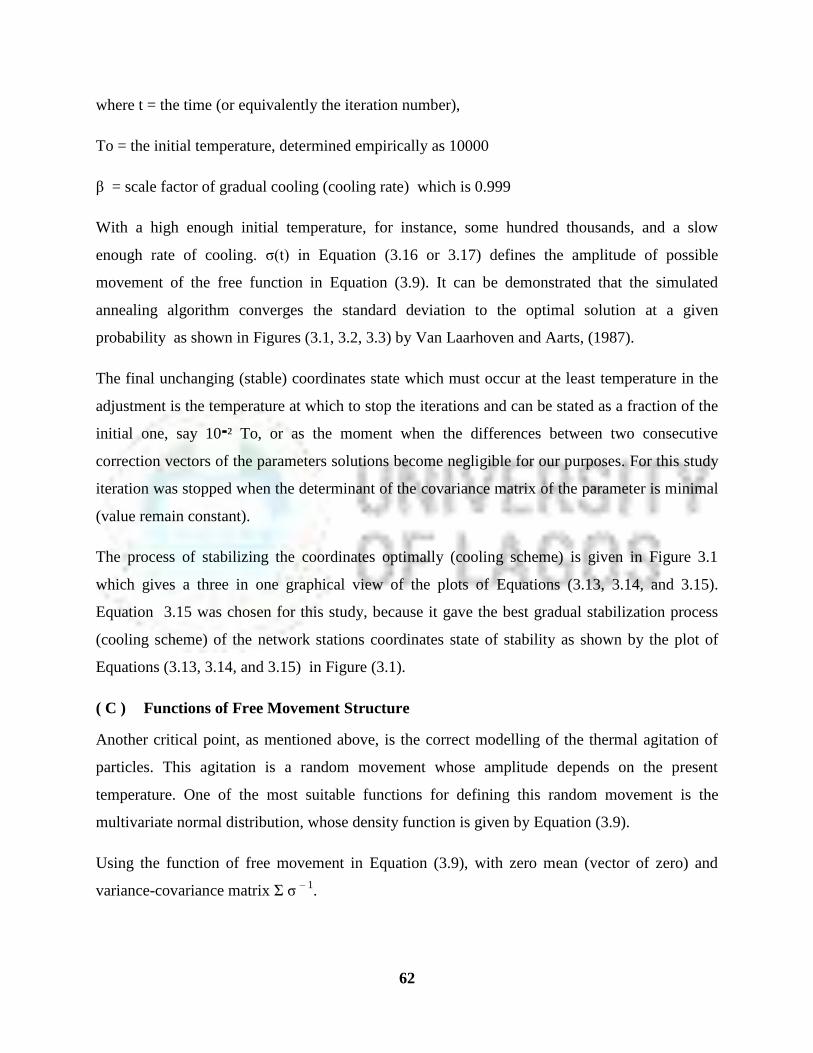
62
where t = the time (or equivalently the iteration number),
To = the initial temperature, determined empirically as 10000
β = scale factor of gradual cooling (cooling rate) which is 0.999
With a high enough initial temperature, for instance, some hundred thousands, and a slow
enough rate of cooling. σ(t) in Equation (3.16 or 3.17) defines the amplitude of possible
movement of the free function in Equation (3.9). It can be demonstrated that the simulated
annealing algorithm converges the standard deviation to the optimal solution at a given
probability as shown in Figures (3.1, 3.2, 3.3) by Van Laarhoven and Aarts, (1987).
The final unchanging (stable) coordinates state which must occur at the least temperature in the
adjustment is the temperature at which to stop the iterations and can be stated as a fraction of the
initial one, say 10²־ To, or as the moment when the differences between two consecutive
correction vectors of the parameters solutions become negligible for our purposes. For this study
iteration was stopped when the determinant of the covariance matrix of the parameter is minimal
(value remain constant).
The process of stabilizing the coordinates optimally (cooling scheme) is given in Figure 3.1
which gives a three in one graphical view of the plots of Equations (3.13, 3.14, and 3.15).
Equation 3.15 was chosen for this study, because it gave the best gradual stabilization process
(cooling scheme) of the network stations coordinates state of stability as shown by the plot of
Equations (3.13, 3.14, and 3.15) in Figure (3.1).
( C ) Functions of Free Movement Structure
Another critical point, as mentioned above, is the correct modelling of the thermal agitation of
particles. This agitation is a random movement whose amplitude depends on the present
temperature. One of the most suitable functions for defining this random movement is the
multivariate normal distribution, whose density function is given by Equation (3.9).
Using the function of free movement in Equation (3.9), with zero mean (vector of zero) and
variance-covariance matrix Σ σ – 1
.
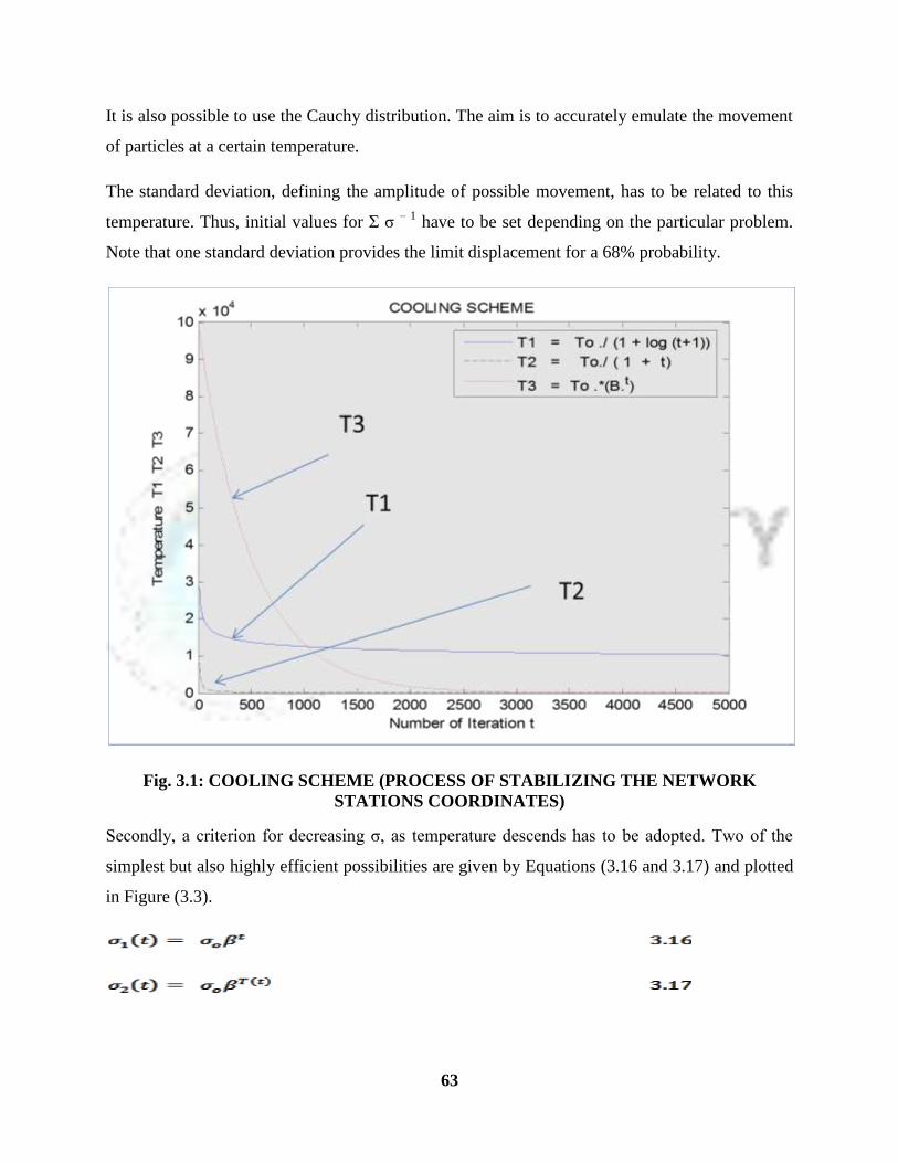
63
It is also possible to use the Cauchy distribution. The aim is to accurately emulate the movement
of particles at a certain temperature.
The standard deviation, defining the amplitude of possible movement, has to be related to this
temperature. Thus, initial values for Σ σ – 1
have to be set depending on the particular problem.
Note that one standard deviation provides the limit displacement for a 68% probability.
Fig. 3.1: COOLING SCHEME (PROCESS OF STABILIZING THE NETWORK
STATIONS COORDINATES)
Secondly, a criterion for decreasing σ, as temperature descends has to be adopted. Two of the
simplest but also highly efficient possibilities are given by Equations (3.16 and 3.17) and plotted
in Figure (3.3).

64
For an initial value σo, a factor β, a temperature T and time t (or equivalently iteration number)
are involved to determine the successive standard deviation of the amplitude of the free
movement function. Consequently, ∆xi displacement is a random one derived from Equation
(3.9) using equation (3.15) together with Equations (3.16) or (3.17) if the new point is located
inside the acceptable domain define by the objective function and the acceptance criteria below,
otherwise ∆xi is zero.
Fig. 3.2: GRAPH OF FUNCTION OF FREE MOVEMENTS OF THE NETWORK
STATIONS COORDINATES
(D). Objective Function and Acceptance Criteria.
The aim of the algorithm (least squares part) mentioned in Section 3.2.1 is to find the global
optimum of a function that defines the goodness of the network design. This function f(xi ) stated

65
in Equation (3.7) or equivalently Equation (3.8) for our purposes – is known as the objective
function.
At first, we can think of admitting every new point xi that betters the previous function value and
rejecting every one that makes it worse. This was the initial approach of the simulated annealing
method (Metropolis et al, 1953). Nevertheless, in some cases the algorithm may fall into local
optimum and not be able to escape if only aided by successive standard deviations subject to the
acceptance criterion in Equation (3.18) only.
Fig. 3.3: PLOT OF THE NETWORK STANDARD DEVIATION SCHEME

66
Here in equation (3.19), the application of a modified criterion can be of more interest; if the new
point provides a better objective function then it is accepted, otherwise the new point (with a
worse solution) is accepted with certain probability P, in order to be able to escape from local
minima. Otherwise we can admit every previous point xi that betters the function value and reject
every one that makes it worse. Expression for the acceptance probability (p) of worse solutions
can be as simple as a given fixed value; for instance values such as 0.2, 0.1, 0.05, 0.01
probability level can be used. Another much more sophisticated possibility, continuing with
thermo dynamical analogies is Boltzman‟s distribution given by equation (3.20).
p takes into consideration the amount of worsening (correction matrix) and the temperature
(stations energy state). This introduces a new problem since the variation range of the objective
function (f (xi + 1 ) - f(xi )) may not correspond to the order of the temperature, and so the
increment f (xi + 1 ) - f(xi ) has to be properly scaled, hence p is chosen empirically, (Pardalos
and Romeijn, 2002).
Equations (3.1 to 3.20) are introduced into the main program of the adjustment to minimize the
determinant of the covariance matrix of the solution matrix thereby minimizing the volume of
the error hyper ellipsoid in the solution.
3.3 ERROR ELLIPSE
It has been shown in equation 2.42 that the least squares estimate of the adjusted parameters X is
given for the general case as:
X = -N -1
U;
where: N=ATPA; U= A
TPL
b;
N = normal coefficient matrix. The unbiased estimate of the covariance matrix of adjusted
parameters is given by:

67
3.21
N-1
= weight coefficient matrix and is denoted by Q i.e. Q = N-1
.
x is an error matrix since standard errors associated with the adjusted parameters may be
estimated from its diagonal elements. The geometries interpretation of the error matrix may be
illustrated by the quadratic form
(Rainsford, 1949; Rainsford, 1957 and Paul, 1999).
which represents the equation of a hyper ellipsoid (multiaxial ellipsoid) centre in
m-dimensional space, where m is the number of parameters (Hamilton, 1964).
When β = 1 we have an ellipsoid of standard deviation which may be projected on the (x,y) plane
to obtain a standard ellipse whose equation is given by Richardus (1966) as:
o2 is a-posteriori variance of unit weight
The weight coefficient matrix Q(2x2) is given by
3.24
x (λ) and y(φ) are the two adjusted vectors of parameters contained in the vector X
68
The equation of the ellipse may be written in terms of the elements of the N coefficient matrix; N
is given for 2 parameters by:
3.27
By making the following substitution in Equation 3.23;
We have equations (3.28 and 3.29)
Graphically the standard ellipse is defined as the ellipse to which the sides of a rectangle given
by Equations (3.28 and 3.29) are tangents (Figure 3.4).
There are several possible ellipses of different orientations (and centered at x,y) which can be
drawn tangentially to the rectangle defined by Equations (3.28 and 3.29). It is therefore
important to derive formulas which will assist us in defining the semi-major and minor axes as
well as the orientation of the axes of the ellipse. Let us consider an orthogonal transformation of
x,y system into a U, V system as follows.
U = xcos + sin 3.30
V = -xsin + cos 3.31
(Biddle, 1958; Baarda, 1968 and Ayeni, 2003)
where is the angle between u- and x- axes. According to the law of propagation of errors
(Ayeni, 2001); given:
oxxxxyyxyxyxx
yqxyqxqqqq
222
2ˆ)2(
)(
1
NNDD
nq
D
nq
D
nq yyxyxx )(det,,, 221222
cossin
sincos,G
v
uZ
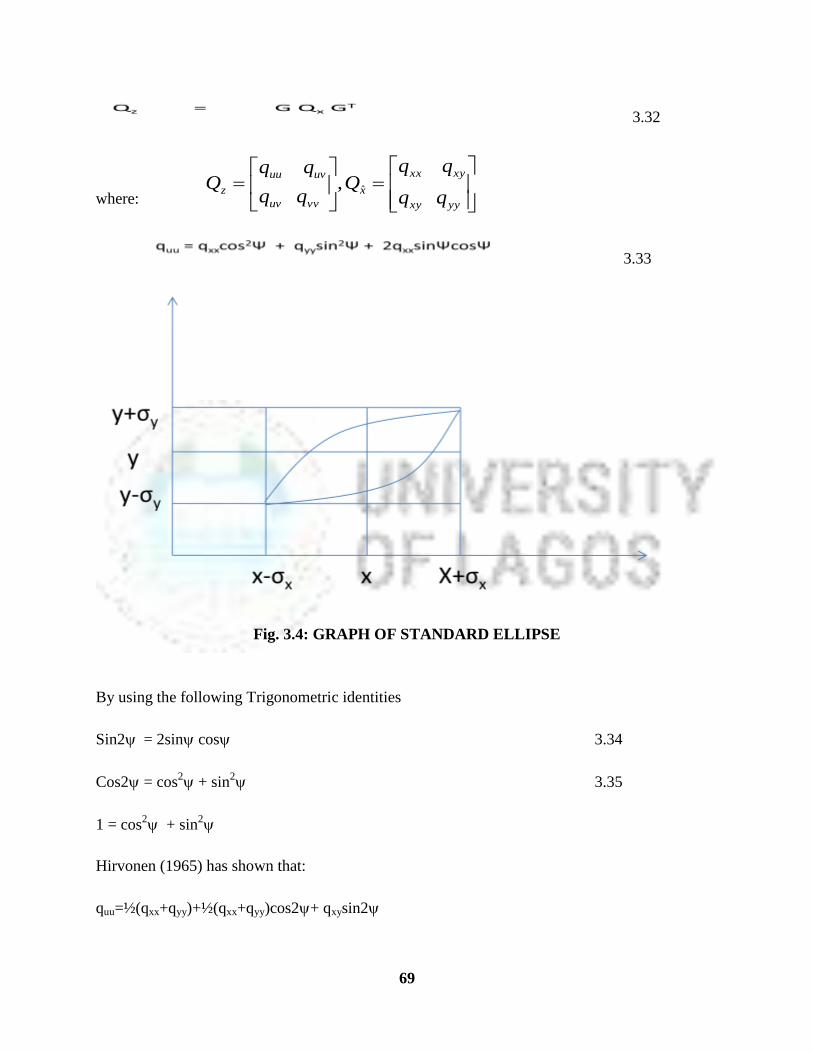
69
3.32
where:
3.33
Fig. 3.4: GRAPH OF STANDARD ELLIPSE
By using the following Trigonometric identities
Sin2 = 2sin cos 3.34
Cos2 = cos2 + sin
2 3.35
1 = cos2 + sin
2
Hirvonen (1965) has shown that:
quu=½(qxx+qyy)+½(qxx+qyy)cos2+ qxysin2
yyxy
xyxx
x
vvuv
uvuu
zqq
qqQ
qqQ ˆ,
70
3.36
Therefore the parameter for ellipse orientation is given by Equation (3.37) as:
3.37
3.38
3.39
where H =
quu=½(qxx+ qyy – H) 3.40
(for minimum)
Similarly from:
qvv = qvv cos2 Ψ–2qxysinΨcosΨ + qxxsin
2 Ψ
it can be shown that:
qvv=½(qxx+qyy– H) 3.41
(for maximum)
The semi-major and minor axes of the error ellipse (parameters for the size of the ellipse) are
therefore defined by Equations (3.42 and 3.43)
3.42
3.43
02sin)(2cos2
yyxxxy
uu qqqq
yyxx
xy
q
22tan
H
qxy22sin
H
qq yyxx 2cos
uuou q ˆ
vvov q ˆ
xyyyxx qqq 22 4)(
71
The resultant value (σuv ) of Equations (3.42) and (3.43), which represent the radial distance error
of each station coordinates can be derived from Equations (3.42 and 3.43) as given by equation
(3.44) .
σuv = (u2 + v
2)½ 3.44
These axes and their orientation may also be computed directly from the covariance matrix. Two
characteristics of error ellipse must be noted. x2
+ y2 are invariant under the orthogonal
transformation so also is x2y
2 - xy
2
i.e. x2
+ y2 = u
2 + v
2
x2y
2 - xy
2 = u
2v
2 - uv
2
If xx= yy , then xy =0, and therefore the error ellipse becomes a circle.

72
CHAPTER FOUR
RESULTS AND ANALYSIS
4.1 RESULTS
All results in this study had passed through statistical testing during the course of adjustment.
The simulated annealing method which is based on the least square approach had also
incorporated statistical algorithm that ensures the following (Section 3.2):
(i) Functions of free movement structure which is a multivariate normal distribution function.
(ii) Objective function and acceptance criteria structure which was incorporated into the function
of free movement to compute the correction vectors of the parameters at a given probability level
(95% confidence level) and hence, the residuals, positional corrections, the error ellipses values,
the standard error in azimuths and distances of all lines in the network. The ATPV matrix after
adjustment is equal to zeroes, this denotes that the residual matrix of the adjusted observation
only contain white random noise.
The a-posteriori variance of unit weight computed from the adjustment, at an acceptance criteria
of 95% probability level was found to be equal to 1meter. This represents the statistical network
standard error of 1 sigma ( and shall be used for the analysis of the distribution of the
network stations geometry.
The use of the simulated annealing method had in the adjustment had help to minimize the
determinant of the covariance matrix of the solution matrix, thereby minimizing the volume of
the error hyper ellipsoid in the solution.
Paired sample statistical test was carried out with the use of SPSS software on the extracted
absolute error values of the 33 stations used in 1977 and their corresponding values in this study
at 95% confidence level. The result is shown in Table (4.2.5b) and Figure (4.2.5a).
The results of the network adjustment and plots are discussed under the following sub –sections:

73
4.1.1 Newly Arranged old Network Data and Result Formats
Intelligently arranged old network data, results from computations and plots were achieved in
this study and discussed in section (4.1).
4.1.1.1 Newly Arranged old Network Data Format
The structure of the newly arranged old network data comprises 1, 054 Triangles, with 515
Stations Identity (Tables 4.1a – c). 3162 lines identity and angles values (Table 4.1b), and 3162
network triangle angles in Tables ( 4.1c). Samples of the newly structured network data format
with details are given respectively in Appendices (IIa, IIb, and IIc). This triangular arrangement
applies to all forms of information on lines, angles, azimuths, station coordinates, residual
values, station correction vectors, and so on (Section 3.1.3 ). The sample graphical view of the
arrangement of the stations is shown in Figure 4.1a
Table 4.1a: SAMPLE TRIANGULARLY ARRANGED STATIONS ID
OF THE NETWORK
TRIANGLE S/N STATION 1 STATION 2 STATION 3
1 K52 K44 A50
1054 N138 N135 N133
Table 4.1b: SAMPLE TRIANGULARLY ARRANGED STATION - STATION/LINES
OF THE NETWORK
TRIANGLE S/N LINE 1 LINE 2 LINE 3
1 K52 - K44 K44 - A50 A50 - K52
1054 N138 - N135 N135 - N133 N133 - N138

74
Table 4.1c SAMPLE TRIANGULARLY ARRANGED ANGLES OF
THE NETWORK ( deg min sec)
TRIANGLE
SR NO ANGLE 1(deg min sec) ANGLE 2(deg min sec) ANGLE 3(deg min sec)
1 59º 52' 57.3623'' 60º 02' 20.8878'' 60º 04' 41.7500''
1054 60º 44' 40.393'' 65º 53' 24.3873'' 53º 21' 55.2200''
Figure 4.1a show a sample of the network plot for any required section of the network, such as
lines, error ellipse plot, residual plot, station correction plot, and so on.
Fig. 4.1a: PLOT OF NETWORK SAMPLE TRIANGULAR STRUCTURE
4.1.1.2 Assessment of the Instruments used/Date of Observation of the Nigerian Horizontal
Geodetic Network
Table 4.1d shows the different instruments used from 1929 to the time of adjustment in 1977.
They are relatively close in least count reading and the deficiency of any of these instrument
were compensated for by the number of rounds of measurements. This consequently created no

75
significant difference between the type of instrument and the date of observation as can be seen
in sample Table (4.1e) with details in Appendices (X). Here the absolute error ellipse values of
the network stations were tabulated in ascending order with type of instrument/date of
observation.
Table 4.1d: INSTRUMENTS USED FOR THE NIGERIAN
HORIZONTAL GEODETIC NETWORK.
TYPE OF SURVEY OBSERVED
ANGLES
INSTRUMENT
SCALE CHECKS
INSTRUMENT
AZIMUTHS INSTRUMENT
DOS TRAVERSE 1‟‟ THEODOLITE
READING ON 8
ZEROES
S.E. = 1‟‟
TELLUROMETER
DISTANCES
51 USABLE LINES OF
TRIANGULATION NET
S.E. = 3 PPM
12TH
PARALLEL
TRAVERSE 2‟‟ THEODOLITE
(WILD T4)
S.E. = 0.70‟‟
GEODIMETER
DISTANCES
46 LINES OF 12TH
PARALLEL
TRAVERSE
S.E. = 2 PPM
2‟‟ THEODOLITE (T4)
23 AZIMUTHS
TRIANGULATION
NETWORK 4‟‟ THEODOLITE
(WILD T3)
READING ON (10 -
20) ZEROES
S.E. = 0.72‟‟
INVAR TAPED BASES
(INVAR WIRES)
USED FOR THE
TRIANGULATION NET
S.E. = 1 PPM
8 OLD AZIMUTHS
REMEASURED
8‟‟ MICROMETER &
4‟‟ THEODOLITE (T3)
8 NEW AZIMUTHS :
8‟‟ MICROMETER and 4‟‟
THEODOLITE (T3)

76
Table 4.1e: NETWORK ASSESSMENT BASED ON INSTRUMENTS STANDARD
DEVIATIONS/YEAR OF OBSERVATION (where applicable)
S/N
ERROR ELLIPSE
VALUE IN
ASCENDING ORDER
(meter)
YEAR
OBSERVED
STANDARD
ERROR OF
ANGLES
(second)
CHAIN/ STANDARD ERROR
IN SCALE CHECKS (PPM)
Chain ID/
S.e.( Azimuth in Second)
Date observed
1 6.04899210414509E-02 '1929-1935' '0.75 -0.77' 'N5', 0.67 'N5', 1.00, 1912'
2 7.85708063404021E-02 '1929-1935' '0.75 -0.77' 'N3', 0.67 'N3', 1.00, 1912'
5 8.57794637219177E-02 '1929-1935' '0.75 -0.77' 'N1', 0.67 'N1-N2, 1.00, 1912'
8 1.08049128289698E-01 '1929-1935' '0.75 -0.77' 'N2', 0.67 'N2'
9 1.08180564119912E-01 '1930-1937' '0.92' 'L39' 'L39-L41, 1.00, 1938'
10 1.09854275072479E-01 '1937' '0.92' 'L37' 'L37'
11 1.13371500413491E-01 '1929-1935' '0.75 -0.77' 'N10-N12, 0.96, N10-N14, 0.67 'N10-N12, 1.00, 1963'
15 1.29346292880717E-01 '1935' '0.75' 'R47' R47-N127,1.00, 1969'
158 3.45171339803536E-01 '1967-1971' '1.00' 'ML52, 3.00' 'ML52'
160 3.47261829144649E-01 '1967-1971' '1.00' 'ML308, 3.00' 'ML308'
506 2.96097513511009E+00 '1967-1971' '0.70' 'CFL11, 2.00'
'CFL11-CFL10, 1.00,
1968'
507 3.01507821965987E+00 '1967-1971' '0.70' 'CFL17, 2.00'
'CFL17-CFL16, 1.00,
1969'
514 3.41360888872390E+00 '1967-1971' '0.70' 'CFL24, 2.00'
'CFL24-CFL23,
1.00,1969'
515 4.82062729063526E+00 '1967-1971' '0.70' 'CFL37, 2.00' 'CFL37'

77
4.1.2 RESULTS OF THE RESIDUAL VECTOR (V) AFTER ADJUSTMENT
The Residual Vector (V) of all observations (angles, distances, azimuths) in the entire network
were computed and plotted as discussed in Sections (2.1.1, 2.1.2 and 2.1.3) to provide a
graphical view of the magnitude of the corrections applied to each observation during the
adjustment. The numerical values whose units are in radian are arranged in ascending order with
their corresponding line identities for all the 3162 lines in the 1054 triangles that made up the
network.
Table (4.1.2a) shows a sample of the residual matrix while the details are given in the
Appendices (III). The graphical plot reveals the magnitude of this residuals (Figure 4.1.2a).
Figure 4.1.2a reveal the size of residuals shown as bars, which represent the amount of
corrections effected to the original observables such as angles, azimuths and scale checks
throughout the network. It can also be seen that numerical values of the residual and their
corresponding sizes of bars for the CFL‟s stations are relatively smaller than others (Table 4.1.2a
and (Figure 4.1.2a). This is because the residual vector formed from the linearised observation
equations, contain more of observations from the triangulation network (an observation
appearing in two or more triangles) than those from the traverse lines. Consequently these
residual corrections (V) from the CFL‟s observations yielded a corresponding position correction
values. The number of time a line appears as bar is the number of time such a line was used in
the network adjustment.

78
Table 4.1.2a ASSESSMENT OF THE SAMPLE NETWORK RESIDUAL MATRIX
S/N OF
LINES/OBSERVATIONS
STATION ID OF
LINES
V MATRIX OF OBSERVATIONS
(radian)
1 ML453XL451 -1.32727861241487E-04
2 R48R47 -9.12734779968862E-05
3 ML451ML403 -8.87450817614267E-05
4 ML54ML53 -7.93193635187504E-05
5 B12B9 -7.91263456432537E-05
6 ML201XL202 -7.58267630321441E-05
7 ML656ML403 -7.18591405053288E-05
1599 L45L27 -8.49110319592170E-09
1600 R42R3 -6.85095221256699E-09
1601 CFL24CFL23 2.52732832055954E-08
1602 CFL14CFL13 3.62725573499121E-08
3155 N42L56 6.47364477112486E-05
3156 A46A42 6.60515085080113E-05
3157 ML502XL453 6.72911136471098E-05
3158 L1L3 6.82468014508886E-05
3159 N128R48 7.03178221369891E-05
3160 L23D2 7.34825231312190E-05
3161 ML705XL453 7.81416569281016E-05
3162 ML456ML453 1.67093443878418E-04

79
Figure 4.1.2a: PLOT OF V (RESIDUALS) MATRIX OF ADJUSTED OBSERVATIONS
OF ALL STATIONS/LINES (3162 lines) IN THE NETWORK
(Charts could not show all stations identity due to scale)
Figure 4.1.2b shows the size of residual (V) represented as bars along the Twelfth Parallel
Traverse (CFL) stations of the network. These bars reveal the number of observation at that point
and their corresponding correction. For the CFL, the observations comprise scale checks,
azimuths and angles.
Figure 4.1.2c shows the contribution of redundancy in triangulation method of survey. More
residual (bars) are revealed for the triangulation stations (Figure 4.1.2c) than the traverse
Network (CFL‟s) in Figure (4.1.2b), thereby providing better estimates of residual corrections of
the observables. Most of the redundant observations are angles.
-0.00008
-0.00006
-0.00004
-0.00002
0
0.00002
0.00004
0.00006
0.00008
0.0001M
L45
3X
L45
1
R4
7N
12
8
E15
E13
C3
9C
40
D2
2D
20
ML6
51
E1
A4
9K
30
CFL
26
CFL
27
XB
15
2X
B1
53
R4
6R
51
CFL
27
CFL
28
D1
0D
12
N1
39
N2
5
F23
F22
F8M
R5
52
V matrix(radian)
V matrix(rad)
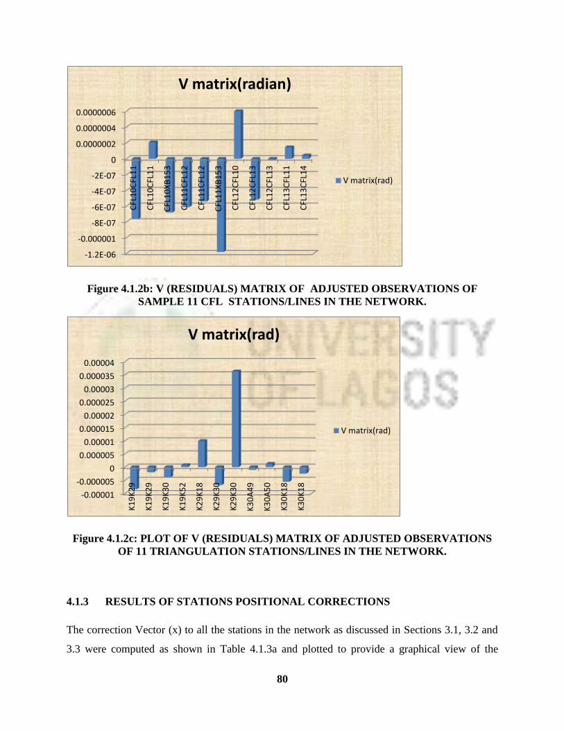
80
Figure 4.1.2b: V (RESIDUALS) MATRIX OF ADJUSTED OBSERVATIONS OF
SAMPLE 11 CFL STATIONS/LINES IN THE NETWORK.
Figure 4.1.2c: PLOT OF V (RESIDUALS) MATRIX OF ADJUSTED OBSERVATIONS
OF 11 TRIANGULATION STATIONS/LINES IN THE NETWORK.
4.1.3 RESULTS OF STATIONS POSITIONAL CORRECTIONS
The correction Vector (x) to all the stations in the network as discussed in Sections 3.1, 3.2 and
3.3 were computed as shown in Table 4.1.3a and plotted to provide a graphical view of the
-1.2E-06
-0.000001
-8E-07
-6E-07
-4E-07
-2E-07
0
0.0000002
0.0000004
0.0000006
CFL
10
CFL
11
CFL
10
CFL
11
CFL
10
XB
15
3
CFL
11
CFL
12
CFL
11
CFL
12
CFL
11
XB
15
3
CFL
12
CFL
10
CFL
12
CFL
13
CFL
12
CFL
13
CFL
13
CFL
11
CFL
13
CFL
14
V matrix(radian)
V matrix(rad)
-0.00001
-0.000005
0
0.000005
0.00001
0.000015
0.00002
0.000025
0.00003
0.000035
0.00004
K1
9K
29
K1
9K
29
K1
9K
30
K1
9K
52
K2
9K
18
K2
9K
30
K2
9K
30
K3
0A
49
K3
0A
50
K3
0K
18
K3
0K
18
V matrix(rad)
V matrix(rad)
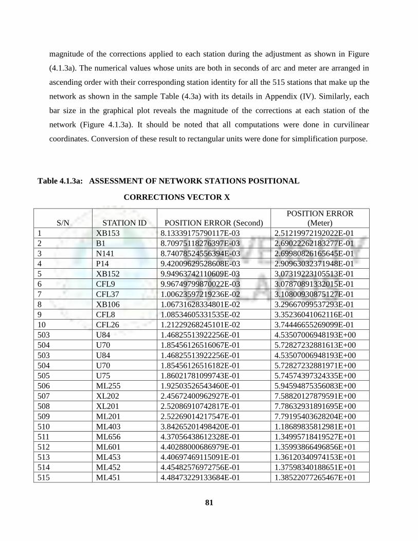
81
magnitude of the corrections applied to each station during the adjustment as shown in Figure
(4.1.3a). The numerical values whose units are both in seconds of arc and meter are arranged in
ascending order with their corresponding station identity for all the 515 stations that make up the
network as shown in the sample Table (4.3a) with its details in Appendix (IV). Similarly, each
bar size in the graphical plot reveals the magnitude of the corrections at each station of the
network (Figure 4.1.3a). It should be noted that all computations were done in curvilinear
coordinates. Conversion of these result to rectangular units were done for simplification purpose.
Table 4.1.3a: ASSESSMENT OF NETWORK STATIONS POSITIONAL
CORRECTIONS VECTOR X
S/N STATION ID POSITION ERROR (Second)
POSITION ERROR
(Meter)
1 XB153 8.13339175790117E-03 2.51219972192022E-01
2 B1 8.70975118276397E-03 2.69022262183277E-01
3 N141 8.74078524556394E-03 2.69980826165645E-01
4 P14 9.42009629528608E-03 2.90963032371948E-01
5 XB152 9.94963742110609E-03 3.07319223105513E-01
6 CFL9 9.96749799870022E-03 3.07870891332015E-01
7 CFL37 1.00623597219236E-02 3.10800930875127E-01
8 XB106 1.06731628334801E-02 3.29667099537293E-01
9 CFL8 1.08534605331535E-02 3.35236041062116E-01
10 CFL26 1.21229268245101E-02 3.74446655269099E-01
503 U84 1.46825513922256E-01 4.53507006948193E+00
504 U70 1.85456126516067E-01 5.72827232881613E+00
503 U84 1.46825513922256E-01 4.53507006948193E+00
504 U70 1.85456126516182E-01 5.72827232881971E+00
505 U75 1.86021781099743E-01 5.74574397324335E+00
506 ML255 1.92503526543460E-01 5.94594875356083E+00
507 XL202 2.45672400962927E-01 7.58820127879591E+00
508 XL201 2.52086910742817E-01 7.78632931891695E+00
509 ML201 2.52269014217547E-01 7.79195403628204E+00
510 ML403 3.84265201498420E-01 1.18689835812981E+01
511 ML656 4.37056438612328E-01 1.34995718419527E+01
512 ML601 4.40288000686979E-01 1.35993866496856E+01
513 ML453 4.40697469115091E-01 1.36120340974153E+01
514 ML452 4.45482576972756E-01 1.37598340188651E+01
515 ML451 4.48473229133684E-01 1.38522077265467E+01

82
Figure 4.1.3a: BAR CHART OF ALL POSITIONAL CORRECTIONS APPLIED TO
THE 515 STATIONS IN THE NETWORK
(Charts could not show all stations identity due to scale of plot).
Figure 4.1.3b: SOME OF THE XL AND ML SECONDARY STATIONS OF THE
NETWORK WITH LARGER POSITIONAL CORRECTIONS,
0.00E+00
2.00E+00
4.00E+00
6.00E+00
8.00E+00
1.00E+01
1.20E+01
1.40E+01
XL4
53
MR
55
0
ML3
08
XL4
51
XL2
51
ML7
05
ML2
55
XL2
02
XL2
01
ML2
01
ML4
03
ML6
56
ML6
01
ML4
53
ML4
52
ML4
51
POSITION CORRECTION (m)
POSITION ERROR (m)
0.00E+00
2.00E+00
4.00E+00
6.00E+00
8.00E+00
1.00E+01
1.20E+01
1.40E+01X
B1
53
R1
4
N1
25
F26
K4
4
C1
8
A2
9
L22
C2
5
B9
A1
7
L4 R4
3
POSITION CORRECTION (m)
POSITION ERROR (m)
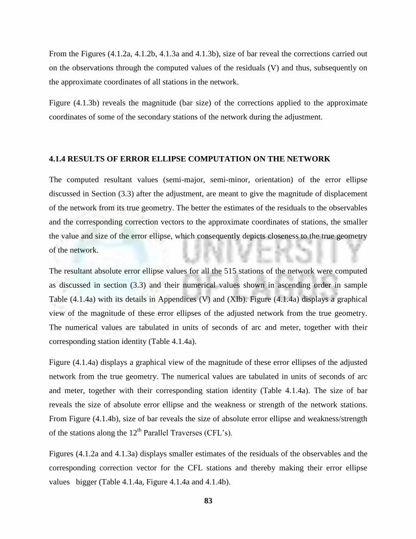
83
From the Figures (4.1.2a, 4.1.2b, 4.1.3a and 4.1.3b), size of bar reveal the corrections carried out
on the observations through the computed values of the residuals (V) and thus, subsequently on
the approximate coordinates of all stations in the network.
Figure (4.1.3b) reveals the magnitude (bar size) of the corrections applied to the approximate
coordinates of some of the secondary stations of the network during the adjustment.
4.1.4 RESULTS OF ERROR ELLIPSE COMPUTATION ON THE NETWORK
The computed resultant values (semi-major, semi-minor, orientation) of the error ellipse
discussed in Section (3.3) after the adjustment, are meant to give the magnitude of displacement
of the network from its true geometry. The better the estimates of the residuals to the observables
and the corresponding correction vectors to the approximate coordinates of stations, the smaller
the value and size of the error ellipse, which consequently depicts closeness to the true geometry
of the network.
The resultant absolute error ellipse values for all the 515 stations of the network were computed
as discussed in section (3.3) and their numerical values shown in ascending order in sample
Table (4.1.4a) with its details in Appendices (V) and (XIb). Figure (4.1.4a) displays a graphical
view of the magnitude of these error ellipses of the adjusted network from the true geometry.
The numerical values are tabulated in units of seconds of arc and meter, together with their
corresponding station identity (Table 4.1.4a).
Figure (4.1.4a) displays a graphical view of the magnitude of these error ellipses of the adjusted
network from the true geometry. The numerical values are tabulated in units of seconds of arc
and meter, together with their corresponding station identity (Table 4.1.4a). The size of bar
reveals the size of absolute error ellipse and the weakness or strength of the network stations.
From Figure (4.1.4b), size of bar reveals the size of absolute error ellipse and weakness/strength
of the stations along the 12th
Parallel Traverses (CFL‟s).
Figures (4.1.2a and 4.1.3a) displays smaller estimates of the residuals of the observables and the
corresponding correction vector for the CFL stations and thereby making their error ellipse
values bigger (Table 4.1.4a, Figure 4.1.4a and 4.1.4b).
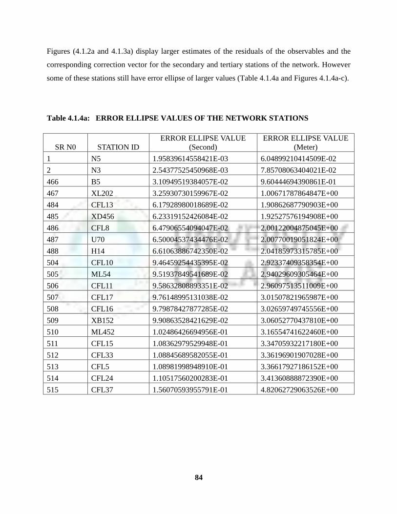
84
Figures (4.1.2a and 4.1.3a) display larger estimates of the residuals of the observables and the
corresponding correction vector for the secondary and tertiary stations of the network. However
some of these stations still have error ellipse of larger values (Table 4.1.4a and Figures 4.1.4a-c).
Table 4.1.4a: ERROR ELLIPSE VALUES OF THE NETWORK STATIONS
SR N0 STATION ID
ERROR ELLIPSE VALUE
(Second)
ERROR ELLIPSE VALUE
(Meter)
1 N5 1.95839614558421E-03 6.04899210414509E-02
2 N3 2.54377525450968E-03 7.85708063404021E-02
466 B5 3.10949519384057E-02 9.60444694390861E-01
467 XL202 3.25930730159967E-02 1.00671787864847E+00
484 CFL13 6.17928980018689E-02 1.90862687790903E+00
485 XD456 6.23319152426084E-02 1.92527576194908E+00
486 CFL8 6.47906554094047E-02 2.00122004875045E+00
487 U70 6.50004537434476E-02 2.00770019051824E+00
488 H14 6.61063886742350E-02 2.04185973315785E+00
504 CFL10 9.46459254435395E-02 2.92337409358354E+00
505 ML54 9.51937849541689E-02 2.94029609305464E+00
506 CFL11 9.58632808893351E-02 2.96097513511009E+00
507 CFL17 9.76148995131038E-02 3.01507821965987E+00
508 CFL16 9.79878427877285E-02 3.02659749745556E+00
509 XB152 9.90863528421629E-02 3.06052770437810E+00
510 ML452 1.02486426694956E-01 3.16554741622460E+00
511 CFL15 1.08362979529948E-01 3.34705932217180E+00
512 CFL33 1.08845689582055E-01 3.36196901907028E+00
513 CFL5 1.08981998948910E-01 3.36617927186152E+00
514 CFL24 1.10517560200283E-01 3.41360888872390E+00
515 CFL37 1.56070593955791E-01 4.82062729063526E+00
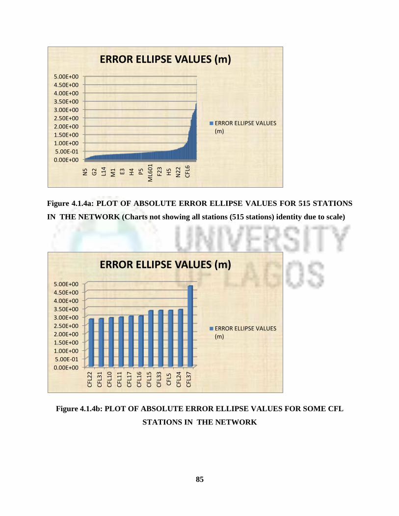
85
Figure 4.1.4a: PLOT OF ABSOLUTE ERROR ELLIPSE VALUES FOR 515 STATIONS
IN THE NETWORK (Charts not showing all stations (515 stations) identity due to scale)
Figure 4.1.4b: PLOT OF ABSOLUTE ERROR ELLIPSE VALUES FOR SOME CFL
STATIONS IN THE NETWORK
0.00E+00
5.00E-01
1.00E+00
1.50E+00
2.00E+00
2.50E+00
3.00E+00
3.50E+00
4.00E+00
4.50E+00
5.00E+00N
5
G2
L14
M1 E3 H4
P5
ML6
01
F23
H5
N2
2
CFL
6
ERROR ELLIPSE VALUES (m)
ERROR ELLIPSE VALUES(m)
0.00E+00
5.00E-01
1.00E+00
1.50E+00
2.00E+00
2.50E+00
3.00E+00
3.50E+00
4.00E+00
4.50E+00
5.00E+00
CFL
22
CFL
31
CFL
10
CFL
11
CFL
17
CFL
16
CFL
15
CFL
33
CFL
5
CFL
24
CFL
37
ERROR ELLIPSE VALUES (m)
ERROR ELLIPSE VALUES(m)

86
Figure 4.1.4c: CHART SHOWING SOME ML, XL, XD and XB SECONDARY
STATIONS WITH THEIR ABSOLUTE ERROR ELLIPSE VALUES IN THE
NETWORK
4.1.5 RESULTS OF RELATIVE ERROR ELLIPSE (RELATIVE GEOMETRY)
COMPUTATION
Table 4.1.5a shows the sample network relative error ellipse values in Section (3.3) of all
lines/stations in their ascending order with its details in Appendix (VI). It shows a very close
agreement with the absolute error ellipse values of stations in the network. The size of ellipse
reveals the relative weakness/strength along each line or station to station as well as the relative
geometry of all stations in the network. From Table 4.1.5a, it can be seen that the CFL‟s and
some of the secondary ML‟s and XL‟s stations have weaker geometry closure. The reason for
this might be due to the lower precisions of observations within the affected chains.
Figure 4.1.5a displays the network relative error ellipse plot of all lines/stations. It shows a very
close agreement with the absolute error ellipse plot (Figure 4.1.4a) of stations in the network.
The size of ellipse reveals the relative weakness/strength along each line or station to station as
well as the relative geometry of all stations in the network. From Figure 4.1.5a, it can be seen
that the CFL‟s and some of the secondary ML‟s, XL‟s stations have weaker geometry closure as
0.00E+00
5.00E-01
1.00E+00
1.50E+00
2.00E+00
2.50E+00
3.00E+00
3.50E+00
XL2
02
ML2
ML3
52
ML7
05
XD
45
6
XB
15
3
XD
70
2
YC2
02
XB
10
6
ML5
4
XB
15
2
ML4
52
ERROR ELLIPSE VALUES (m)
ERROR ELLIPSE VALUES(m)
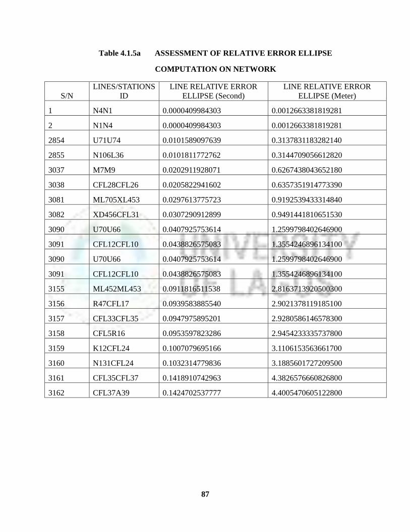
87
Table 4.1.5a ASSESSMENT OF RELATIVE ERROR ELLIPSE
COMPUTATION ON NETWORK
S/N
LINES/STATIONS
ID
LINE RELATIVE ERROR
ELLIPSE (Second)
LINE RELATIVE ERROR
ELLIPSE (Meter)
1 N4N1 0.0000409984303 0.0012663381819281
2 N1N4 0.0000409984303 0.0012663381819281
2854 U71U74 0.0101589097639 0.3137831183282140
2855 N106L36 0.0101811772762 0.3144709056612820
3037 M7M9 0.0202911928071 0.6267438043652180
3038 CFL28CFL26 0.0205822941602 0.6357351914773390
3081 ML705XL453 0.0297613775723 0.9192539433314840
3082 XD456CFL31 0.0307290912899 0.9491441810651530
3090 U70U66 0.0407925753614 1.2599798402646900
3091 CFL12CFL10 0.0438826575083 1.3554246896134100
3090 U70U66 0.0407925753614 1.2599798402646900
3091 CFL12CFL10 0.0438826575083 1.3554246896134100
3155 ML452ML453 0.0911816511538 2.8163713920500300
3156 R47CFL17 0.0939583885540 2.9021378119185100
3157 CFL33CFL35 0.0947975895201 2.9280586146578300
3158 CFL5R16 0.0953597823286 2.9454233335737800
3159 K12CFL24 0.1007079695166 3.1106153563661700
3160 N131CFL24 0.1032314779836 3.1885601727209500
3161 CFL35CFL37 0.1418910742963 4.3826576660826800
3162 CFL37A39 0.1424702537777 4.4005470605122800

88
Figure 4.1.5a: STATIONS WITH LARGER RELATIVE ERROR ELLIPSE VALUES IN
THE NETWORK (Chart could not show all line (3162 lines) identities due to scale).
4.1.5.1 Results of Standard Error in Azimuths
The Network Standard Error in Azimuths of all lines are shown in ascending order along with
their station to station identity in the sample result in Table 4.1.5b with details in Appendices
(VII) and Figures (4.1.5b, 4.1.5c, and 4.1.5d). The network strength/weakness of azimuths
(orientation) of all lines can be deduced in ascending order in this table.
The 12th
parallel traverse (CFL‟s stations) and the secondary/tertiary stations (ML‟s, XB‟s,
XD‟s, XL‟s) are weaker in orientation compared to the other stations.
0.00E+005.00E-011.00E+001.50E+002.00E+002.50E+003.00E+003.50E+004.00E+004.50E+00
N4
N1
C2
3C
25
K4
0K
38
C8
C9
N3
4N
66
M2
M1
E4E6
N1
0N
14
L13
L15
G2
G4
D1
9D
22
N1
40
N3
5
RELATIVE ERROR ELLIPSE SIZES OF LINES (m)
RELATIVE ERROR ELLIPSESIZEOF LINES (m)

89
Table 4.1.5b SAMPLE NETWORK STANDARD ERROR OF AZIMUTHS OF LINES
S/N
STATIONS/LINES
ID STANDARD ERROR OF AZIMUTH (Second)
1 R37R35 1.04273651424594E-04
2 R37R35 1.04273651424594E-04
3 R35R37 1.04273651424594E-04
4 E15L38 1.31406589778790E-04
450 N136N131 1.56261808528142E-03
451 N131N136 1.56261808528142E-03
3114 CFL35CFL34 4.60676384754674E-02
3115 CFL35CFL34 4.60676384754674E-02
3118 CFL11CFL12 4.78302222671061E-02
3119 ML54XL301 4.86920209597843E-02
3121 ML54ML53 5.31106006786564E-02
3122 ML54ML53 5.31106006786564E-02
3123 ML452XL202 5.32611317019209E-02
3124 XL202ML452 5.32611317019209E-02
3125 A36ML54 5.41316652479105E-02
3153 CFL17N127 1.17710866557099E-01
3154 CFL6XB106 1.20992821839288E-01
3155 CFL32CFL33 1.24009632199593E-01
3156 CFL33XD702 1.41806320987866E-01
3157 XD702CFL33 1.41806320987866E-01
3158 CFL32CFL30 1.44612575096434E-01
3159 CFL34XD702 1.45666908976288E-01
3160 XD456CFL31 1.46459880605601E-01
3161 CFL31CFL30 1.47615953546203E-01
3162 CFL30CFL31 1.47615953546203E-01

90
Figure 4.1.5b: CHART OF STANDARD ERRORS IN AZIMUTHS OF THE NETWORK
(Chart could not show all lines (3162 line)) identities due to scale).
Figure 4.1.5c: CHART SHOWING SOME CFL STATIONS/LINES WITH LARGER
STANDARD ERROR IN AZIMUTHS VALUES IN THE NETWORK.
0.00E+00
2.00E-02
4.00E-02
6.00E-02
8.00E-02
1.00E-01
1.20E-01
1.40E-01
1.60E-01
R3
7R
35
N4
N2
E11
E12
L54
L52
K4
7B
17
A7
A3
N1
14
N1
10
L26
L25
N4
0N
42
R3
5R
36
H1
2N
26
N1
08
N1
04
P1
5P
16
AZIMUTH STANDARD ERROR(Sec)
AZIMUTH STANDARDERROR(Sec)
0.00E+00
2.00E-02
4.00E-02
6.00E-02
8.00E-02
1.00E-01
1.20E-01
1.40E-01
1.60E-01
CFL
8C
FL7
R4
7C
FL1
7
N1
27
CFL
17
CFL
17
N1
27
CFL
6X
B1
06
CFL
32
CFL
33
CFL
33
XD
70
2
XD
70
2C
FL3
3
CFL
32
CFL
30
CFL
34
XD
70
2
XD
45
6C
FL3
1
CFL
31
CFL
30
CFL
30
CFL
31
STANDARD ERROR IN AZIMUTH (Sec)
STANDARD ERROR INAZIMUTH (Sec)
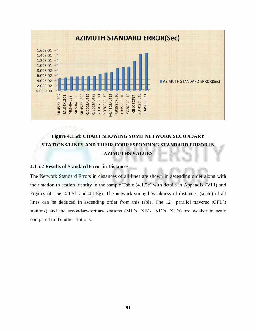
91
Figure 4.1.5d: CHART SHOWING SOME NETWORK SECONDARY
STATIONS/LINES AND THEIR CORRESPONDING STANDARD ERROR IN
AZIMUTHS VALUES
4.1.5.2 Results of Standard Error in Distances
The Network Standard Errors in distances of all lines are shown in ascending order along with
their station to station identity in the sample Table (4.1.5c) with details in Appendix (VIII) and
Figures (4.1.5e, 4.1.5f, and 4.1.5g). The network strength/weakness of distances (scale) of all
lines can be deduced in ascending order from this table. The 12th
parallel traverse (CFL‟s
stations) and the secondary/tertiary stations (ML‟s, XB‟s, XD‟s, XL‟s) are weaker in scale
compared to the other stations.
0.00E+002.00E-024.00E-026.00E-028.00E-021.00E-011.20E-011.40E-011.60E-01
ML4
53
XL2
02
ML5
4X
L30
1
ML5
4M
L53
ML5
4M
L53
ML4
52
XL2
02
XL2
02
ML4
52
XL2
01
ML4
52
XD
70
2C
FL3
1
XD
70
2C
FL3
2
ML4
52
ML4
53
XB
15
3C
FL1
0
XB
15
2C
FL1
0
YC2
02
CFL
15
XB
10
6C
FL7
XD
70
2C
FL3
3
XD
45
6C
FL3
1
AZIMUTH STANDARD ERROR(Sec)
AZIMUTH STANDARD ERROR(Sec)

92
Table 4.1.5c SAMPLE NETWORK STANDARD ERROR OF DISTANCES OF LINES
S/N STATIONS/LINES STANDARD ERROR OF DISTANCE(m) 1
N4N3 3.69374907436008E-11
2 N3N4 3.69374907436008E-11
3 N3N1 1.82970257816117E-10
4 N1N3 1.82970257816117E-10
450 A10E18 1.70886118939992E-09
451 F2F1 1.71099756278415E-09
3114 XD702CFL31 5.85573434284588E-07
3115 ML54ML53 6.02206891875569E-07
3116 ML54ML53 6.02206891875569E-07
3117 A36ML54 6.15973692027048E-07
3122 CFL14CFL12 7.52493998813762E-07
3123 ML452ML453 7.56546576160243E-07
3124 CFL32XD702 8.11472732421762E-07
3125 XD702CFL32 8.11472732421762E-07
3153 CFL17N127 2.11317241160263E-06
3154 CFL6XB106 2.19806869672546E-06
3155 CFL32CFL33 2.30671225593517E-06
3156 CFL33XD702 3.02269071611815E-06
3157 XD702CFL33 3.02269071611815E-06
3158 CFL32CFL30 3.16104201450632E-06
3159 CFL34XD702 3.17961574121035E-06
3160 XD456CFL31 3.21444886672260E-06
3161 CFL31CFL30 3.26582106323275E-06
3162 CFL30CFL31 3.26582106323275E-06
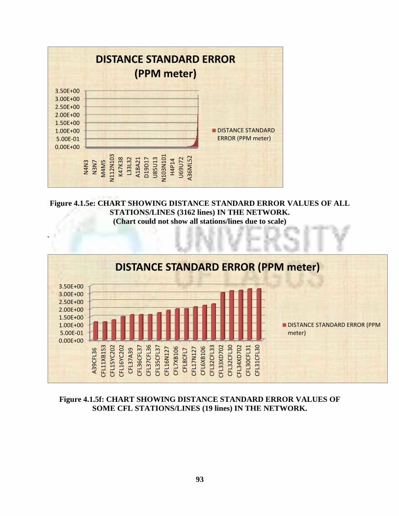
93
Figure 4.1.5e: CHART SHOWING DISTANCE STANDARD ERROR VALUES OF ALL
STATIONS/LINES (3162 lines) IN THE NETWORK.
(Chart could not show all stations/lines due to scale)
`
Figure 4.1.5f: CHART SHOWING DISTANCE STANDARD ERROR VALUES OF
SOME CFL STATIONS/LINES (19 lines) IN THE NETWORK.
0.00E+005.00E-011.00E+001.50E+002.00E+002.50E+003.00E+003.50E+00
N4
N3
N3
N7
M4
M5
N1
12
N1
03
K4
7K
38
L33
L32
A1
8A
21
D1
9D
17
U8
5U
13
N1
03
N1
01
H4
P1
4
U6
9U
72
A3
6M
L52
DISTANCE STANDARD ERROR (PPM meter)
DISTANCE STANDARDERROR (PPM meter)
0.00E+005.00E-011.00E+001.50E+002.00E+002.50E+003.00E+003.50E+00
A3
9C
FL3
6
CFL
11
XB
15
3
CFL
15
YC2
02
CFL
16
YC2
02
CFL
37
A3
9
CFL
36
CFL
37
CFL
37
CFL
36
CFL
35
CFL
37
CFL
16
N1
27
CFL
7X
B1
06
CFL
8C
FL7
CFL
17
N1
27
CFL
6X
B1
06
CFL
32
CFL
33
CFL
33
XD
70
2
CFL
32
CFL
30
CFL
34
XD
70
2
CFL
30
CFL
31
CFL
31
CFL
30
DISTANCE STANDARD ERROR (PPM meter)
DISTANCE STANDARD ERROR (PPMmeter)

94
Figure 4.1.5g: CHART SHOWING DISTANCE STANDARD ERROR VALUES OF
SOME SECONDARY STATIONS/LINES (16 lines) IN THE NETWORK.
4.2 ANALYSIS OF RESULTS
The analysis of results is divided into six subsections in accordance with the objectives of this
research. A close view of each of the bar charts in section 4.1 clearly shows the tabulated range
of values against the stations/lines being considered at any given time.
It should be noted that due to the small scale of plotting used in the charting of each of the
Figures 4.1.2a, 4.1.3a, 4.1.4a, 4.1.5a, 4.1.5b, and 4.1.5e which represents the whole network
plot, most of the stations/lines identities are hidden in the individual plots, but shown in the other
figures depending of the chosen area of interest/analysis.
4.2.1 Analysis of the Network residuals of Observations (V) after the Adjustment
Before Network Adjustment
The observations used in this adjustment were eliminated of gross errors and the following
results were achieved.
Triangular closure (TC) lies in the region (-3.6 < TC < 3.7) seconds (Appendices Ia).
Mean Triangular closure is 0.9358633776118294 second (Appendices Ia).
0.00E+00
5.00E-01
1.00E+00
1.50E+00
2.00E+00
2.50E+00
3.00E+00
3.50E+00
XB
15
3C
FL1
0
ML4
52
XL2
02
XL2
02
ML4
52
XL2
01
ML4
52
XB
15
2C
FL1
0
ML4
53
XL2
02
YC2
02
CFL
15
ML2
01
ML2
ML2
ML2
01
XL2
01
ML2
ML1
ML2
01
XB
10
6C
FL7
R4
7C
FL1
7
N1
27
CFL
17
XD
70
2C
FL3
3
XD
45
6C
FL3
1
DISTANCE STANDARD ERROR (PPM meter)
DISTANCE STANDARD ERROR(PPM meter)
95
After network Adjustment
Residual vector (V) after adjustment is shown in Table 4.1.2a and appendix (III), V matrix of
size (3162 by 1) ranges between {-7.8182E-05 and - 9.7688E-05} radian for both angles and
distances and this can be categorized into V < ± 1 second for all angles and V < ± 1m for all
distances.
Figure 4.1.2a shows the plot of the network residuals values in radian against their corresponding
stations/lines used in the adjustment. Its distribution gave higher and better estimates of the
residuals at the extreme ends and lower estimates of the residuals towards the middle of the
charts, thereby revealing and relating stations/lines identity and their corresponding residuals.
It seems that the triangulation stations lies at the extreme ends of the chart with higher and better
estimates of residuals (Figure 4.1.2c), the secondary stations follows, while the CFL
stations/lines occupies the middle section of the (Figure 4.1.2b) chart and thus denoting least
estimate of residuals in the network.
Triangulation stations involve interconnected lines from other triangles stations. It provides the
opportunity of using a given station/line observation as many times as it appears in a network,
thereby providing redundant observations for the adjustment of such station/line. This in turn
would give higher/better estimates of the residual V as seen on line K29K30 in Figure (4.1.2c).
Sample of the residual values is shown in Table (4.1.2a) and the Appendix (III) for all the
stations.
Other stations/lines like the CFL traverse stations configuration which contributes less redundant
observations as against the triangulation stations configuration during adjustment gave
lower/poorer estimates of V, while the secondary stations/lines gave a better estimates of the
residuals than the CFL stations/lines as observed in Figure 4.1.2a
4.2.2 Analysis of the Network Stations Position Correction (x) after the adjustment
The resultant of 515 stations position corrections of size (515 by 2) lies in the region (0.25122m
- 5.74574m) for all stations, with the exception of the 10 tertiary stations (9 ML-chains stations
and 1 XL-chain station) which lies in the region of {5.94595m and 13.85221} as shown in Table
96
(4.1.3a) and Appendix (IV). Triangulation stations/lines with large redundant observations gave
higher/better estimates of x. Other stations/lines like the CFLs with less redundant observations
gave lower/poorer estimates of x, while the secondary stations/lines with higher redundant
observations produced a larger/better estimates of x as shown in Figures (4.1.2a, b, and c.)
where same line bar is repeated, especially in triangulation where an observation can appear in
two or more triangles during adjustment.
Figure 4.1.3a shows the plot of the network positional corrections (x) due to the residuals values
against their corresponding stations/lines used in the adjustment. Its distribution gave higher and
better estimates of x towards the extreme right, lower estimates of the x towards the extreme left
of the chart, thereby revealing and relating stations/lines identity and their corresponding
positional correction values.
It can be seen that the triangulation stations lies at the extreme right of the chart with higher and
better positional corrections (Figure 4.1.3a), the secondary stations follows, while the CFL
stations/lines occupies the extreme left of chart and thus denoting least estimate of residuals in
the network.
Sample of the positional corrections values is shown in Table (4.1.3a) and the Appendix (IV) for
all the stations. Figure (4.1.3b) shows the distribution of the positional corrections in the
secondary stations/lines of the network.
4.2.3 Analysis of the Network Error Ellipse (Geometry) after the Adjustment
Stations resultant error ellipse values (radial error) lies in the region ( 0.061 – 4.821) meters
(Table 4.1.4a). Triangulation stations/lines with large redundant observations gave higher/better
estimates of V and x and hence a lower values of resultant error ellipse values (radial error) as
shown in Tables (4.1.2a, 4.1.3a, 4.1.4a), Figures (4.1.2a, 4.1.3a, 4.1.4a) and Appendix (XIb)
Other stations/lines CFLs with less redundant observations gave lower/poorer estimates of V and
positional corrections and hence higher values of error ellipse (radial eerror) (Tables 4.1.2a,
4.1.3a, 4.1.4a) and (Figures 4.1.2a, 4.1.3a, 4.1.4a and Appendix (XIb)). The absolute/relative
error ellipse values of any station/line directly denotes the relative geometry of such station/line
in the network.

97
Table (4.1.4a) and Figure (4.1.4a and Appendix (XIb)) shows the plot of the network absolute
error ellipse values against their corresponding stations used in the adjustment. Its distribution
gave higher estimates at the extreme right and lower estimates at the extreme left of the charts,
thereby revealing and relating stations identity and their corresponding absolute error values.
It can be seen that the triangulation stations lie at the extreme left of the chart with smaller and
better estimates/stronger section in geometry of the network stations (Figure 4.1.4a), while the
CFL and some of the secondary stations occupy the extreme right of the chart and thus signifying
higher estimate/weaker section in the network geometry. Details of the distribution is in
Appendix (V) and Appendix (XIb).
Figure (4.1.4b) and Figure (4.1.4c) reveals the magnitudes of the network absolute error ellipses
for the CFL and the secondary stations respectively.
Plan for strengthening the network can be achieved as follows:
The Network a-posteriori variance of unit weight after adjustment was computed to be 1 meter,
and this represents the standard deviation of the network ( ⏞ = 1 meter). Classification can thus
be made of the network error ellipse values as a factor of the standard deviation of the network to
ascertain likely possible number of stations that would need re-observation so as to strengthen
the network.
The number of stations that fall outside each class of the network standard deviation
classification thus represents the network stations that would need to be re-observed, so as to
strengthen the network. For example the last 49 stations in Table 4.1.4a, appendix (V), Appendix
(XIb and (XII a) would need a re-observation to attained a standard deviation of ≤ ( 1 ⏞ ) as
shown in Table 4.5d. 90.5% of the present network stations fall within error ellipse values of ≤
( 1 ⏞ ).
4.2.4 Analysis of the Network Relative Error Ellipse (Relative Geometry)
Stations relative error ellipse size vector (Relative E.Lx) showed that 94.2% ( error ellipse values
of stations ≤ 2 meter) of stations standard deviations lies within 2-sigma network standard
deviation. The relative error ellipse values range within (1.26634E-03 – 4.40055) meter and of
size (3162 by 1).
98
Table (4.1.5a) and Figure (4.1.5a) shows the plot of the network relative error ellipse values in
meters against their corresponding stations/lines identity used in the adjustment. Its distribution
gave higher and better estimates towards the extreme ends and lower estimates towards the
extreme left of the charts.
4.2.4.1 Analysis of the Network Standard Error in Azimuths (Orientation)
Station – Station (Line) Standard error (S.e.) in azimuth lies in the region
( 0.00010" – 0.14762") as in Table (4.1.5b).and Appendix (VI).
Table (4.1.5b) and Figure (4.1.5b) showed the plot of the network standard errors in azimuth
values against their corresponding stations/lines used in the adjustment. Its distribution gave
higher estimates at the extreme right and lower estimates at the extreme left of the charts, thereby
revealing and relating stations/lines identity and their corresponding standard error in azimuths.
It can be seen that the triangulation stations lie at the extreme left of the chart with smaller and
better estimates/stronger section in orientation of the lines in the network (Figure 4.1.5b), while
the CFL and some of the secondary stations/lines occupy the extreme right of the chart and thus
signifying higher estimate/weaker section in orientation of the lines in the network. Details of the
distribution is in Appendix (VII).
Figure (4.1.5c) and Figure (4.1.5d) reveals the magnitude of the standard error in azimuths for
the CFL and the secondary stations/lines in the network respectively.
4.2.4.2 Analysis of the Network Standard Error in Distances (Scale)
Station – Station (Line) Standard error (S.e.) in Distances lies in the region
( 0.00037 – 3.26582) PPM in meters as in Table (4.1.5c).
Table (4.1.5c) and Figure (4.1.5e) shows the plot of the network standard errors in distance
values against their corresponding stations/lines used in the adjustment. Its distribution gave
higher estimates at the extreme right and lower estimates at the extreme left of the charts, thereby
revealing and relating stations/lines identity and their corresponding standard error in distances.

99
It can be seen that the triangulation stations lie at the extreme left of the chart with smaller and
better estimates/stronger section in scale of the lines in the network (Figure 4.1.5e), while the
CFL and some of the secondary stations/lines occupy the extreme right of the chart and thus
signifying higher estimate/weaker section in scale of the lines in the network. Details of the
distribution are shown in Appendix (VIII).
Figure (4.1.5f) and Figure (4.1.5g) reveals the magnitude of the standard error in distances for
the CFL and the secondary stations/lines in the network respectively.
It can be deduced that the Nigerian Horizontal Geodetic Network Standard error in distances,
falls in the acceptable specification of a Primary Network of 1/100,000 (Table 2.1.5.1.1 and
Appendix VIII).
4.2.4.3 Analysis of the Network Standard Deviation
The classification of the Network Standard Deviation is given in Table 4.2.4.3a
Table 4.2.4.3a CLASSIFICATION /ASSESSMENT OF NETWORK A- POSTERIORI
VARIANCE OF UNIT WEIGHT (NETWORK STANDARD DEVIATION ⏞ = 1 meter)
NETWORK STANDARD
DEVIATION ( ⏞ = 1 meter)
CLASSIFICATION
NUMBER OF
NETWORK STATIONS
WITHIN A CLASS
NUMBER OF
NETWORK
STATIONS OUTSIDE
A CLASS
NUMBER OF NETWORK
STATIONS WITHIN A
CLASS PERCENTAGE
(%)
≤ ( 1 ⏞ ) 466 49 90.5%
≤ ( 2 ⏞ ) 485 30 94.2%
≤ ( 3 ⏞ ) 506 9 98.3%
≤ ( 4 ⏞ ) 514 1 99.8%
≤ ( 5 ⏞ ) 515 NONE 100%
It can therefore be deduced that the Nigerian Horizontal Geodetic Network Standard error in
azimuths, falls in the acceptable specification of a primary network which is 0.4seconds (Table
2.1.5.1.2).
4.2.5 Statistical Paired Sample test analysis of the error ellipse values of the 33 Stations of
the Network used in 1977 and their corresponding values in 2009 adjustment.

100
The results of the error ellipse values in the 1977 and 2009 adjustments are shown in Table
(4.2.5a). The result of the statistical paired sample test of the data in Table (4.2.5a) shown in
Table (4.2.5b) at 95% confidence level reveals that the misclosure in the Geometry of the 33
stations have been reduced by 36% (Figure 4.2.5a) in the 2009 adjustment.

101
Table 4.2.5a: COMPARISON OF ERROR ELLIPSE VALUES FOR 33 STATIONS USED
IN 1977 AND THEIR CORRESPONDING VALUES IN 2009 ADJUSTMENT
RESULT OF ERROR ELLIPSE
PARAMETER IN 1977
ADJUSTMENT
RESULT OF ERROR
ELLIPSE PARAMETER
IN 2009 ADJUSTMENT
S/N STN ID error ellipse values (m) error ellipse values (m)
1 A50 0.339705755 0.532768419
2 B9 0.502493781 0.31087458
3 C1 0.914002188 0.365302356
4 C18 0.517397333 0.446354699
5 C30 0.651920241 0.293212354
6 C32 0.498196748 0.450049134
7 C6 0.915478017 0.378443483
8 D15 0.660681466 0.40139855
9 D34 0.468614981 0.367893166
10 D5 0.714212853 0.315136174
11 E13 0.829276793 0.380398444
12 E3 0.412310563 0.359156202
13 F1 0.587962584 0.39253392
14 H1 0.686221539 0.483649711
15 H11 0.452769257 0.304410309
16 H12 0.632534584 0.300091819
17 K11 0.428018691 0.40582027
18 K17 0.322024844 0.496442103
19 L19 0.758221603 0.264783661
20 L33 0.296984848 0.199516126
21 L8 1.098362417 0.28215929
22 M1 0.735527022 0.330514462
23 N104 0.240831892 0.526722116
24 N12 0.403112887 0.210405589
25 N124 0.428018691 0.360634383
26 N38 0.304138127 0.380111136
27 P15 0.538144962 0.784287696
28 P9 0.651152824 0.341421165
29 R34 0.81467785 0.439254982
30 R5 0.702922471 0.293145068
31 U67 0.731095069 0.365039143
32 U71 0.759275971 0.381462273
33 U78 0.915478017 0.506848498

102
Table 4.2.5b: PAIRED SAMPLE TEST ON THE EXTRACTED ABSOLUTE
ERROR VALUES OF 33 STATIONS
IN THE 1977 AND 2009 ADJUSTMENTS AT 95% CONFIDENCE LEVEL
Fig. 4.2.5a: 95% CONFIDENCE LEVEL PLOT OF ABSOLUTE ERROR
ELLIPSE BAR FOR 33 STATIONS
IN THE 1977/2009 ADJUSTMENTS
4.2.6 Comparison of the 515 Stations Coordinates in the 1977 and their corresponding
values in 2009 adjustments.
The results of a sample of the 515 Network stations coordinates in 1977, the change in the
coordinates due to the 2009 adjustment, and the new coordinates are shown in sample Table
4.2.6a with details in Appendices (IX). The plot of the adjusted stations coordinates are shown in
Figure 4.2.6a.
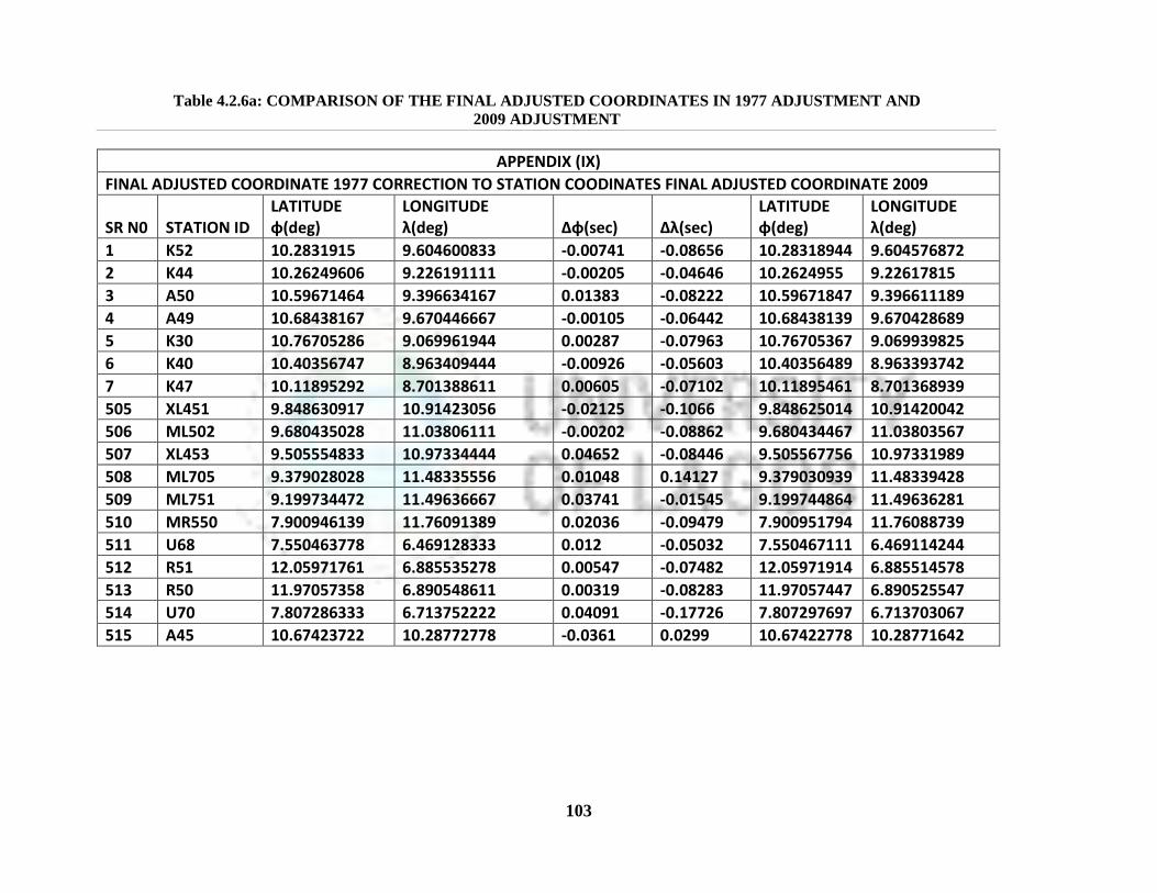
103
APPENDIX (IX)
FINAL ADJUSTED COORDINATE 1977 CORRECTION TO STATION COODINATES FINAL ADJUSTED COORDINATE 2009
SR N0 STATION ID LATITUDE φ(deg)
LONGITUDE λ(deg) ∆φ(sec) ∆λ(sec)
LATITUDE φ(deg)
LONGITUDE λ(deg)
1 K52 10.2831915 9.604600833 -0.00741 -0.08656 10.28318944 9.604576872
2 K44 10.26249606 9.226191111 -0.00205 -0.04646 10.2624955 9.22617815
3 A50 10.59671464 9.396634167 0.01383 -0.08222 10.59671847 9.396611189
4 A49 10.68438167 9.670446667 -0.00105 -0.06442 10.68438139 9.670428689
5 K30 10.76705286 9.069961944 0.00287 -0.07963 10.76705367 9.069939825
6 K40 10.40356747 8.963409444 -0.00926 -0.05603 10.40356489 8.963393742
7 K47 10.11895292 8.701388611 0.00605 -0.07102 10.11895461 8.701368939
505 XL451 9.848630917 10.91423056 -0.02125 -0.1066 9.848625014 10.91420042
506 ML502 9.680435028 11.03806111 -0.00202 -0.08862 9.680434467 11.03803567
507 XL453 9.505554833 10.97334444 0.04652 -0.08446 9.505567756 10.97331989
508 ML705 9.379028028 11.48335556 0.01048 0.14127 9.379030939 11.48339428
509 ML751 9.199734472 11.49636667 0.03741 -0.01545 9.199744864 11.49636281
510 MR550 7.900946139 11.76091389 0.02036 -0.09479 7.900951794 11.76088739
511 U68 7.550463778 6.469128333 0.012 -0.05032 7.550467111 6.469114244
512 R51 12.05971761 6.885535278 0.00547 -0.07482 12.05971914 6.885514578
513 R50 11.97057358 6.890548611 0.00319 -0.08283 11.97057447 6.890525547
514 U70 7.807286333 6.713752222 0.04091 -0.17726 7.807297697 6.713703067
515 A45 10.67423722 10.28772778 -0.0361 0.0299 10.67422778 10.28771642
Table 4.2.6a: COMPARISON OF THE FINAL ADJUSTED COORDINATES IN 1977 ADJUSTMENT AND
2009 ADJUSTMENT
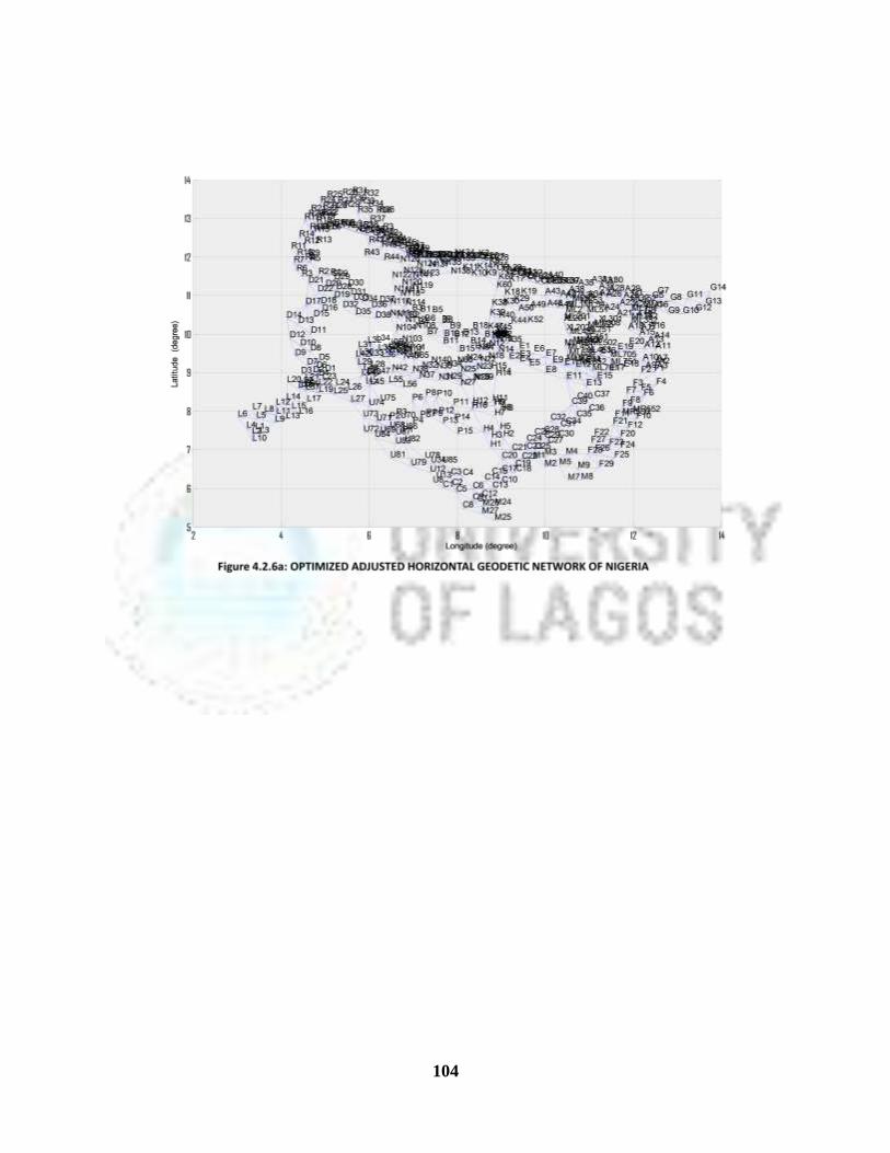
104

105
4.2.7 Analysis of the Summary of the Results in the 1977 and 2009 adjustments.
The Summary of both adjustments are shown in Table (4.2.7a).
Table 4.2.7a COMPARISON OF 1977 & 2009 ADJUSTMENT
S/N SUMMARY OF 1977 ADJUSTMENT SUMMARY OF 2009 ADJUSTMENT
1 Adjustment by observation equation
method.
Least square Phase adjustment was used.
Adjustment by observation equation method.
Least square Optimized Simultaneous
adjustment was used.
2 A posteriori variance of unit weight is
1.17
A posteriori variance of unit weight is 1.0
3 The least element of AT
PV is not zero
while the largest element was 1.02E-09.
All elements of AT
PV are zeroes which
denotes presence of only white random noise
in the adjusted observation.
4 Maximum standard error (S.e.) of
Azimuths after adjustment is 75'' while
that of distance is 546ppm
Maximum S.e of Azimuths after adjustment
is 0.147615953546203'' while that of
distance is 3.26582106323275ppm
5 Standard error of mean for absolute error
ellipse values for 33 lines selected was
3.677E-02
Standard error of mean for absolute error
ellipse values for 33 lines selected was
1.197E-02
6 Standard deviation for the absolute error
ellipse values for the 33 lines used in
1977 was 0.2112
Corresponding Standard deviation for the
absolute error ellipse values of the 33 lines
selected in 2009 was 0.1101
7 Mean for absolute error ellipse values
for the 33 lines selected was 0.6034
Mean for absolute error ellipse values for the
33 lines selected was 0.3833
8 Weakness in the southern part of the
network
Weakness in CFL and few secondary and
tertiary stations of the network.
9 Error analysis not carried on the entire
network.
The standard deviation of network was found
to be 1.0m and 94.2% of the network stations
with error ellipse values ≤ 2 meters represent
2-sigma statistical interval in the network
standard deviation distribution.

106
CHAPTER FIVE
CONCLUSIONS, CONTRIBUTIONS TO KNOWLEDGE AND RECOMMENDATIONS
5.1 CONCLUSIONS.
An optimized holistic adjustment of the Nigerian horizontal geodetic network has been achieved
with a- posteriori variance of unit weight = 1.0 meter, which represents the network
standard deviation (which is an indication of an optimal design and adjustment of the network)
and the product of ATPV matrix being zeroes (which confirms the presence of only white
random noise in the residuals of the adjusted observation) (Table 4.2.7a).
Comparison of the 2009 and 1977 adjustments showed that:
(a) 2009 adjustment has a maximum Standard error (S.e) in Azimuths of
0.147615953546203'' while that of 1977 was 75'' (Figures 4.1.5b –d, Tables 4.1.5b and
4.2.7a), hence the optimized holistic approach used in this study has greatly improved
and revealed the strength of the network in orientation.
(b) 2009 adjustment has maximum Standard errors (S.e) in distance of
3.26582106323275ppm. while that of 1977 was 546ppm (Figures 4.1.5e –g, Table 4.1.5c
and Table 4.2.7a), hence the optimized holistic approach used in this study has greatly
improved and revealed the strength of the network in scale.
(c) 2009 adjustment has an a-posteriori variance of unit weight of 1.0 (an indication of
optimal design of the network) while that of 1977 was 1.17 (Table 4.2.7a).
(d) 2009 adjustment has improved the geometry of the 33 selected stations/lines used for
error ellipse analysis in 1977 by 36% as confirmed by the following values (Table 4.6d):
Standard error of mean: 3.677E-02 (in 1977); 1.197E-02 (in 2009)
Standard deviation: 0.2112 ( in 1977); 0.1101 (in 2009)
Mean: 0.6034 (in 1977); 0.3833 (in 2009).
The study has recovered the lost network data by searching for possible libraries within and
outside the country where the data could be found. Also, the creation of a comprehensive
intelligent database for the whole network which can search, query and perform calculations of
any desired parameters of the network has been achieved. For example the data base can be used
to compute the variance covariance matrix of any control station or the azimuth of any line in the

107
network (Figure 4.1a and Tables 4.1a –f). The products of the database are tabulated in the
appendices. The software for the data base is shown in appendix 1d.
The following Network geometry have been determined in-terms of: the residuals of the
observations (Figures 4.1.2a –c, Table 4.1.2a); positional corrections (Figures 4.1.3a –b, Table
4.1.3a); error ellipse values (Figures 4.1.4a – c, and 4.1.5a; Tables 4.1.4a, 4.1.5a, 4.2.4.3a and
4.2.7a and Appendix XII a, b, c); standard errors in azimuths (Figures 4.1.5b –d; Tables 4.1.5b
and 4.2.7a); and standard errors in distances (Figures 4.1.5e –g; Tables 4.1.5c and 4.2.7a).
The plotting and annotation of any figure in the entire network using the intelligent data base
created have been achieved.
The identified areas of strength/weakness (geometry) in scale and orientation in the network are
as stated below:
(a) The Triangulation section of the Network was found to be relatively less error prone due
to the enormous redundant observations that connected the stations. hence these stations
were more stable than other chains (Figures 4.1.2a, 4.1.2c, 4.1.3a, 4.1.4a, 4.1.4c; Tables
4.1.2a, 4.1.3a, 4.1.4a and 4.1.5a).
(b) Triangulation stations (U70, U68, N26, and H14) which occurred towards the end of their
respective chains, and therefore were connected by few observations were identified as
relatively weaker sections of the triangulation network (Figures 4.1.2a, 4.1.2c, 4.1.3a,
4.1.4a, 4.1.4c; Tables 4.1.2a, 4.1.3a, 4.1.4a and 4.1.5a).
(c) With the exception of a few secondary and tertiary stations (XD456, XL202, XB152,
ML54 and ML452) with error ellipse values > 1m, other secondary and tertiary stations
have error ellipse values < 1 meter. This adjustment has helped to improve the accuracy
of these stations (Figures 4.1.2a, 4.1.3a-b, 4.1.4a, 4.1.4c; Tables 4.1.2a, 4.1.3a, 4.1.4a).
(d) The CFL stations incorporated few observations as compared to the triangulation stations
in the adjustment, therefore giving relatively poorer estimates of its residuals/correction
vectors, as shown in the larger values of error ellipses. The CFL section is therefore the
relatively weaker part of the network (Figures 4.1.2a, 4.1.2b, 4.1.3a, 4.1.4a-b; Tables
4.1.2a, 4.1.3a, 4.1.4a and 4.1.5a).

108
The identified network stations which require upgrade so as to achieve improved network
geometry are listed in order of urgency (Table 4.2.4.3a):
(a) All the CFL section of the network (Tables 4.1.2a, 4.1.3a, 4.1.4a and 4.1.5a);
(b) The following secondary and tertiary stations section of the network: XD456, XL202,
XB152, ML54 and ML452 (Tables 4.1.2a, 4.1.3a, 4.1.4a and 4.1.5a).
(c) The sections towards the end of the triangulation chains, such as: U70, U68, N26, and
H14.
(d) All the other stations of the network are also necessary for upgrade to improve on the
network geometry (Tables 4.1.2a, 4.1.3a, 4.1.4a and 4.1.5a
(e) The network re-strengthening/station upgrade exercise can be classified thus (Table
4.2.4.3a): 49 stations at 1-sigma network standard deviation; 30 stations at 2-sigma
network standard deviation; while at 3-Sigma, 9 stations would be re-observed.
The different computer programs created in this study, such as that of adjustment; error analysis;
and data structure; now form an efficient platform for any future adjustment and study of the
Nigerian Horizontal Geodetic Network (Sections 3.1-3.4). An example is the creation of a
coefficient matrix space' that can help compute the design matrix of any large system, (Appendix
Ic),
This platform comprises:
(a) Network program for the computation of the residual vector of the observations
(Appendix Ic, Figures 4.1.2a –c, and Table 4.1.2a).
(b) Network program for the computation of the positional corrections (Appendix Ic, Figures
4.1.3a –b, Table 4.1.3a)
(c) Network program for the computation of the error ellipse value (positional shift) of
4.81metres (Appendix Ic, Figures 4.1.4a –c, and 4.1.5a; Tables 4.1.4a, 4.1.5a and 4.2.7a).
(d) Network program for the computation of the Standard error in Azimuths (orientations) of
0.147615953546203" (Appendix Ic, Figures 4.1.5b –d; Tables 4.1.5b and 4.2.7a).
(e) Network program for the computation of the Standard error in distance of

109
3.26582106323275ppm (Appendix Ic, Figures 4.1.5e –g; Tables 4.1.5c and 4.2.7a) which
include
Program for plotting and annotating the network triangles (Appendix Ic, Figure 4.2.6a);
Program for plotting and annotating the network residuals (Appendix Ic, Figures 4.1.2a-c);
Program for plotting and annotating the network positions corrections (Appendix Ic, Figures
4.1.3a-b);
Program for plotting and annotating the network absolute and relative error ellipse values
(Appendix Ic, Figures 4.1.4a-c and 4.1.5a);
Program for plotting and annotating the network standard errors in lengths(scales) and
azimuths (orientation), as shown in Appendix Ic, and Figures 4.1.5a-g;
(k) The above subsections (6a – j) would together assist to identify areas of strength/weakness
in the network and consequently allow for the upgrade of the network geometry at a minimal
cost.
There are many important parameters about the Nigerian Horizontal Geodetic Network which
before this study were unknown but now revealed: for example
(a) The network stations position correction is distributed in the range 0.25122m -
13.85221m within the network (Table 4.1.3a).
(b) The Nigerian Horizontal Geodetic Network fulfils the conditions of a primary order
network (94.2% of stations standard deviations fall within 2-sigma network standard
deviation).
The optimized adjusted network plot was not superimposed on the map of Nigeria because it is
not within the scope of this study. If the coordinates of the boundary points with other related
features are known as shown in the old Nigerian network map (Appendix XIII), the intelligent
data base can readily complete the plot accurately.

110
5.2 CONTRIBUTIONS TO KNOWLEDGE.
(1) For the first time in the history of Nigeria, an optimized holistic adjustment of the Nigerian
horizontal geodetic network has been achieved. A- Posteriori variance of unit weight of 1.0 was
achieved which is an indication of an optimal design and adjustment of the network. Also the
ATPV vectors after adjustments are zeroes which confirms the presence of only white random
noise in the residuals of the adjusted observation (Table 4.2.7a). Both confirms the network
reliability.
(2) The areas of strength and weakness in scale and orientation in the Nigerian horizontal
geodetic network have been determined.
(3) A future re-strengthening and re-observation plan of the Nigerian horizontal geodetic
network at different network standard deviations have been achieved and recommended in this
study (Table 4.2.4.3a and Appendix XII a, b, c).
(4). The study has created a generalized network through the creation of a comprehensive
intelligent database for the whole network which can search, query and perform calculations of
any desired parameters of the network. For example you can ask the data base to compute the
variance covariance matrix of any control station or the azimuth of any line in the network
(Figure 4.1a and Tables 4.1a-f).
(5).Through this study, the missing data for Nigerian Horizontal Geodetic Network have been
recovered by searching for possible libraries within and outside the country where the data could
be found (Appendix Ia).
5.3 RECOMMENDATIONS
(1) The findings in this study now provide the foundational platform for the Nigerian geodetic
network, and is therefore recommended to the Federal Government of Nigeria, Nigerian
Institution of Surveyors, Surveyors Council of Nigeria and other stake holders for an immediate
plan on the network re-observation and re-strengthening in order to know the possible trend of
changes like network distortion, that might have taken place especially since the advent of
mineral exploitations in Nigeria.

111
(2) The intelligent data base created in this study would assist accelerating the speed of any
future update/upgrade adjustment and study of the Nigerian Horizontal Geodetic Network.
(3) The transformation parameters of the Nigerian geodetic system should be determined as a
matter of urgency using the result of this adjustment where necessary.
(4) The software written for this study is recommended for use by Survey Department, Surveyors
and other relevant stake holders.
(5) If the Nigerian boundary stations coordinates and other related features are known as shown
in the Nigerian map (Appendix X111), I recommend that, the intelligent data structure created
in this study, be used to accurately complete the plot of the Nigerian map containing the adjusted
network.
The following recommendations are therefore made for further study on the Nigerian geodetic
network:
(6) The incorporation of GPS satellite observations into the network will assist in reducing the
geometric error in the network. This new set of observations can be used for the distortion study
of the Nigerian geodetic network.
(7) Re-observations of the identified weak stations must be carried out with the space satellite
technique on the network to re-strengthen the Nigerian Horizontal Geodetic network. This would
improve the network geometry at a minimal cost.
(8). New observations must be carried out on the entire network alongside other new well
selected stations all over the country, using the space satellite technique to re-strengthen the
network and it‟s distortion study to avert or minimize future disaster.

112
REFERENCES
Allman, J.S. and Hoar G.J. (1973), “Optimisation of Geodetic Networks.” Survey Review vol
XXII No. 167, pp181-207.
Anon, (1936), “Nigeria Survey Department Instructions for Primary Triangulation.” Government
Printer Lagos, pp1-45.
Anon, (1961), “Modern Computing Methods.” Notes on Applied Science No. 16. 2nd
edition.
National Physical Laboratory. H.M.S.O. pp1-170.
Anon, (1971), “Final report of the 12th
Parallel Survey in the Republic of Nigeria.” Corps of
Engineers U.S.A. pp1-217.
Ashkenazi, V. (1967), “Solution and error analysis of large geodetic net-works - 1 Direct
methods.” Survey Review Vol XD No. 146 pp166-173, No. 147 pp194-206.
Ashkenazi, V. (1970), “Adjustment of Control Networks for precise Engineering Surveying.”
Chartered Surveyor Vo1, 102 no. 7 pp314-320
Ashkenazi, V. and Cross, P.A. (1972), “Strength analysis of Block VI of the European
Triangulation.” Bulletin Geodesique pp6-23.
Ashkenazi, V., Cross P.A., Davies M.J.K. and Proctor D.W. {1972), “The Re-adjustment of the
Re-triangulation of Great Britain.” Ordnance Survey Professional papers new series no.
24. pp1-51.
Ashkenazi, V. (1974), “An assessment of the proposed re-adjustment of the North American
Geodetic Control networks, U.N.E Symposium”, Springer Berlin/Heidelberg, pp247-250.
Atilola, O. (1985-86), “Unpublished Lecture notes on Adjustment Computation I.” Department
of Surveying, University of Lagos, pp1-40.
Ayeni, O. O. (1980) “An investigation into the choice of the most appropriate Least Squares
method for position determination” Proceedings of the International Workshop on
Geodetic Positioning.University of Lagos, Nigeria, September 8- 10, 1980, pp99-132.
Ayeni, O. O. (1980) “Adjustment computation by Least Squares” unpublished lecture note,
Department of Surveying, University of Lagos, pp1-35.

113
Ayeni, O.O. (1985) , “ Comparison of least squares of adjustment methods for Geodetic
Level Network.” Proceedings of the NAG conference on Datum Determination in
Nigeria, pp89-93.
Ayeni, O.O. (2001) “ Adjustment and Analysis of Data.“, Lecture notes, Department of
Surveying and Geoinformatics, University of Lagos, pp1-300.
Ayeni, O.O. (2002) “Statistical Adjustment and Analysis of Data (With applications in Geodetic
Surveying and Photogrammetry).“, Lecture notes, Department of Surveying and
Geoinformatics, University of Lagos, pp1-49.
Ayeni, O.O. (2003) “ Adjustment computation” Unpublished Lecture notes (SVY 908)”, Dept.
of Surveying and Geoinformatic, University of Lagos, pp1-55.
Baarda, W. (1968), “A Testing Procedure for Use in Geodetic Networks”, Publication on
Geodesy, Netherlands Geodetic Commission, pp1-97.
Baarda, W., (1977), “Measures for the Accuracy of Geodetic Networks.” IAG Symposium.
Sopron, Hungary pp1-26.
Bagratuni, G. V. (1962), “Course in Spheroidal Geodesy”, translated from Russian to English
language in 1967 by the Translation Division, Foreign Technology, pp1-305.
Bannister, A. and Raymong, S (1972). “Surveying “Published by Pitman Press, London, pp1-89.
Barricelli N. A. (1954), "Esempi numerici di processi di evoluzione". Methodology,pp45-68.
Barricelli, N. A. (1963), "Numerical Testing of Evolution theories, Part II. Preliminary tests
of performance, symbiogenesis and terrestrial life". Acta Biotheoretica (16): pp99-126.
Baudry, B., Franck F., Jean-Marc J. and Yves L. T. (2005), "Automatic Test Case Optimization:
A Bacteriologic Algorithm". IEEE Software: pp76-82.
Berne, J L. and Baselga, S. (2003). “First-order design of geodetic networks using the simulated
annealing method” Springer Berlin Heidelberg, pp47-54.
Biacs, Z, Krakiwsky, E, and Lapucha, D, (1990), “Reliability Analysis of Phase Observations
in GPS Baseline Estimation”, Journal of Surveying Engineering, ASCE, pp204-224.
114
Bies, Robert R; Muldoon, Matthew F; Pollock, Bruce G; Manuck, Steven; Smith, Gwenn and
Sale, Mark E (2006). "A Genetic Algorithm-Based, Hybrid Machine Learning Approach
to Model Selection". Journal of Pharmacodynamics: pp196-221.
Biddle, C.A. (1958), “Textbook of field astronomy.” H.M.S.O pp1-247.
Bomford, G. (1971), “Geodesy.” 3rd
edition. Clarendon, pp1-731.
Bradley, H.E. (1939), “The year 1937 In Nigeria.” Empire Survey Review Vol. V no. 31,
pp50-52
Butler, T.L. (1966), “Draft specifications for the observation of latitudes, longitudes, and
azimuths using the Wild T4.” Unpublished communication, pp1-51.
Calder W. J. (1931), “The Triangulation of Nigeria.” Proceedings of the Empire Survey
Officer‟s Conference 1931. pp 4-21.
Calder W. J. (1936-37), “The survey framework of Nigeria.” Empire Survey Review Vol 111
No 21 pp 386 - 395, No.22 pp 450 – 469, and Vol. IV No. 23 pp 2-12.
Cerny V. (1985), Grafarend (1974) and Baarda (1973), “Application of optimization method
to the famous „Travelling salesman problem‟ Wikipedia 2007, pp1-166.
Cerny, V. (1985), “A thermodynamical approach to the travelling salesman problem: an efficient
simulation algorithm.” Journal of Optimization Theory and Applications 45, pp41-51.
Chang, Y. M., Chen, C. H. and Chen, C.S. (1996), “Optimal observation design of a surveying
artificial neural Geomat Res Aust 64: pp1–16
Charles B. B. (1942) “Surveying” Wiley, New York, pp1-495.
Chedtham, G. (1965), “Textbook of topographical surveying” H.M.S.O. pp1-388.
Choi J. H., (1998) " Evaluation of the Accuracy of the new Primary Precise Geodetic network in
Korea", Earth, Planets and Space, Vol. 50, No.8, pp611-708.
Clark, D. (1965), “Plane and Geodetic Surveying for Engineers” Vol 11 Higher Surveying . 5th
Edition. Constable. Pp1-385.
Close C.A. (1933), “A 50 years retrospect.” Empire Survey Review Vol. 11 No. 8,pp1-30.
Cooper, M.A.R. (1974), “Fundamentals of Survey measurement and analysis.” Crosby
Lockwood Staples pp1-107.

115
Cross, P. A. (1974), “A comparison of modern position control networks with particular
reference to Kenya.” Journal of Geodesy, Springer Berlin/Heidelberg, pp169-180.
Cross, P. A. (1985), “ Numerical methods in network design: In optimization and design of
geodetic networks .” edited by Grafarend and Sanso. Springer: Berlin etc.pp429-435.
Crosby, Jack L. (1973), “Computer Simulation in Genetics.” London John Wiley & Sons, pp1-
492.
Dare, P. (1995), “Optimal Design of GPS Networks Operational Procedures,” Phd. Thesis,
School of Surveying, University of East London.pp1-400.
Dare, P. and Saleh, H. (2000), GPS design: logistic solution optimal and near-optimal methods.
Journal of Geodsy 74(6): pp467–478.
De Normann, A.W.N, (1933), “The year 1931 in Nigeria.” Empire Survey Review XII No. 7
pp44-46.
Dept. of the Army, (1953), ”Topographic Surveying” U.S. Govt. Print off (Washington) pp1-
280.
Even-Tzur, G.,and Papo, H., (1996), “Optimization of GPS Networks by linear programming”,
Empire Survey Review pp537-545.
Even-Tzur, G. (2001) “GPS Vector Configuration Design For Monitoring Deformation
Network in the North of Israel”, The 10th
FIG International Symposium on Deformation
Measurements, Orange, California, USA, pp146-151.
Fajemirokun, F.A. (1988) “ Unpublished Lectures Notes on Geometric Geodesy” Dept. of
Surveying and Geoinformatics, University of Lagos, pp1-40.
Falkenauer E. (1997), “Genetic Algorithms and Grouping Problems.” Chichester,
England: John Wiley & Sons Ltd, pp627-645.
Fentress, S. W. (2005). “Exaptation as a means of evolving complex solutions.” MA
thesis, University of Edinburgh Springer Berlin/ Heidelberg, pp301-309.
Ffox, L. (1964), “An introduction to numerical linear algebra.” Clarendon pp1-328.
FGCC (2006), “Specification of Geodetic Network”, Wikipedia, 2007 pp1-16.

116
Field N. J. (1977), “The adjustment and Strength Analysis of the Primary Triangulation
Network of Nigeria” M.Phil Thesis, University of Nottingham, 1977 pp1-417.
Fogel, D. B. (editor) (1998). Evolutionary Computation: The Fossil Record. New
York: IEEE Press, pp8-14.
Fogel, D. B. (2000). Evolutionary Computation: Towards a New Philosophy of
Machine Intelligence. New York: IEEE Press, pp1-140.
Fogel, D. B (2006), Evolutionary Computation: Toward a New Philosophy of Machine
intelligence, IEEE Press, Piscataway, Third Edition, pp1-372.
Fraser, A. S. (1957). "Simulation of Genetic Systems by Automatic Digital Computers. I.
Introduction", Australian Journal of Biological Sciences 10, pp484-491.
Fraser, A. S. and Donald B. (1970). “Computer Models in Genetics.” New York: McGraw-Hill
pp597-611.
Gazdzicki, J., (1976), “Strength Analysis of Geodetic Control Network”, Bull Geodesique, Paris,
France.
Gerasimeko MD (1997), “First order design of the deformation with the minimal number of
geodetic points and their optimal allocation”. Far East Math Rep 4: pp86–94
Gerasimeko MD, Shestakov NV, Kato T (2000), “On optimal geodetic design for fault-
mechanics studies” .Earth Planet Space 52: pp985–987
Goldberg, David E (1989), “Genetic Algorithms in Search, Optimization and Machine
Learning, “ Kluwer Academic Publishers, Boston, MA pp1-432
Goldberg, David E (2002), “The Design of Innovation: Lessons from and for Competent Genetic
Algorithms,” Addison-Wesley, Reading, MA pp721-739.
Grafarend E (1974), “Optimization of Geodetic” Bulleting Geodetic Science Aff 33: pp351–406
Graferand, E. and Sanso, F. (1986), “Classical first Order Design Problem” Wikipedia, 2007
pp103-123.
Grant, D. B., Blick, G. H, Pearse, M. B., Beavan, R. J. and Morgan P. J.(1999). "The
Development and Implementation of New Zealand geodetic Datum 2000", Presented at
IUGG99 General Assembly, Birmingham UK, 1999, pp18-30.

117
Grushinskiy, N. P. (1963), “The Theory of the Figure of the Earth” translated from Russian to
English in 1969, Hajila AD694748, pp17-78.
Holland J. H. (1975), Adaptation in Natural and Artificial Systems, University of Michigan
Press, pp1-28.
Hong-sic Y. (2001), New Technology for a new century, FIG International Conference,
pp415-423.
Hotline, M. (1935), “The East African Arc III Observations.” Empire Survey Review Vol 111
No. 16 pp77-80
Ingham, A.E. (1975) “Sea Surveying”, Empire Survey Review, pp1-146.
Jagar R. (1988). “Analogies between Geodetic networks and Discrete Elastomechanical
Systems” Series C, rep 342, Journal of Geodesy, Sringer Berlin/Heidelberg, pp1-308.
Jager R.,kaltenbach H. (1990) and Schmitt J. M. (1997), “Introducing Spectra analysis to
Network stiffness” Manual of Geodesy 15: pp302–311.
Johnson and Wyatt (1994), “Application of first order design in Geodynamics Geodetic
Networks” Manual of Geodesy 19: pp309–323
Jordan- Eggert, (1962), “Jordan‟s Handbook of Geodesy”, translation of 8th
edition, 1941 by
Martha W. carta, (U. S. Army Map Service, Washington, D. C.) pp1-124.
Kenya Institute of Surveying and mapping Nairobi, 2000, “Geodetic Report of Kenya” pp1-12
Kirkpatrick, S and Gelatt, C. D. and Vecchi, M. P (1983), “ Optimization by Simulated
Annealing”, Science, Vol 220, Number 4598, pp671-680.
Kjellström, G. (1970). "Optimization of electrical Networks with respect to Tolerance
Costs.". Ericsson Technics (3): pp157-175.
Kjellström, G. (Dec. 1991). "On the Efficiency of Gaussian Adaptation". Journal of
Optimization Theory and Applications. (3): pp589-597
Kjellström, G. (January 1996). "Evolution as a statistical optimization algorithm".
Evolutionary Theory (11): pp105-117.

118
Koza, John (1992), Genetic Programming: On the Programming of Computers by Means of
Natural Selection, MIT Press. ISBN 0-262-11170-5, pp1-387.
Kuang, S., (1996), “Geodetic Network Analysis and Optimal Design”, Ann Arbor Press,
Inc.pp1-368.
Kuang, S. (1996), “An overview of recent work on Network design.” Ann Arbor Press, Inc.
pp1-368.
Land Information New Zealand, (2000) "Specifications for the Installation of GPS
Permanent Tracking Stations, Version 1.0, Office of the Surveyor General, pp1-11.
Legault M. M. (1985) “Surveying” Empire Survey Review, pp1483-1485.
Lindlohr, W. and D. Wells (1985), “GPS Design Using Undifferenced Carrier Phase
Observations”, Manuscripta Geodetica pp1-69.
Mccaw, G.T. (1935), “The two metres: the story of an African foot.” Empire survey review Vol.
9 No. 52 pp96-105.
Metropolis, N., Rosenbluth, A. W., Rosenbluth, M. N., Teller, A. H. andTeller, E (1953).
"Equations of State Calculations by Fast Computing Machines". Journal of Chemical
Physics, 21(6): pp1087-1092.
Michalewicz Z. (1999),”Genetic Algorithms + Data Structures = Evolution
Programs” Springer-Verlag pp1-209.
Mitchell M., (1996), An Introduction to Genetic Algorithms, MIT Press, Cambridge, MA,
pp1-270.
Morley, O.J. (1938), “History of the Minno-Udi-Ilorin series.” Unpublished records of Federal
Surveys Lagos, pp1-46.
Munsey, D.F. (1949), “Base measurement in the Anglo-Egyptian Sudan.” Empire Survey
Review Vol. X No. 74, pp1-34.
Nickerson, B.G. (1978) “A Priori Estimation of Variance for Surveying Observables”:Dept.
of Surveying Engineering, University of New Brunswick Federiction, N.B., Canada
pp1-58.

119
Olliver, J.G. and Clendinning, J. (1970) “Principles of Surveying” 4th
, Ed., vol 1: Plane
Surveying, Empire Survey Review pp1-267.
Omogunloye O.G. (1988), “Optimum number of traverse station between azimuths checks in
A traverse network” Unpublished B.Sc. Project, Dept. of Surveying, University of Lagos
pp1-61.
Omogunloye O.G. (1990) “Quality control in geophysical prospecting” Unpublished M.Sc.
Project,Department. of Surveying and Geoinformatics, University of Lagos, pp1-88.
Ordnance Survey (1967), “History of the retriangulation of Great Britain.” H.N.S.O. pp1-395.
Pardalos P. M.and Romeijn H. E. (2002). “Global Optimization problems” Wikipedia, 2007
pp1-569.
Paul, T. R. J. (1999) " The Need for Dynamic Datum‟s", Geometrics Research
Australasia No. 71, 1999, pp87-102.
Rainsford, H.F. (1949), “Long lines on the Earth: various formulae. ” Empire Survey Review
Vol. X No. 71 and 72 pp19-29.
Rainsford, H.F (1957), “Survey adjustments and least squares.” Constable & Co Ltd. London.
Pp1-326.
Ralph H. (1985) “Guide to Site Surveying” Empire Survey Review, pp1-310.
Richardus, P. (1966), “Project surveying.” Elsevier North Holland pp1-427.
Roeloss, R. (1950), “Astronomy applied to land surveying.” Argue Amsterdam pp1-259.
Saad, A. A. and Elsayed, M. S. 2007. “Simple Model for Improving the Accuracy of the
Egyptian Geodetic Triangulation Network” FIG Working Week, Hong Kong, pp1-24.
Schaffrin, B. (1985), “Aspects of Network Design, Optimization and Design of Geodetic
Networks,” Grafarend and Sanso, editions. Springer – Verlag, Berlin, pp548-597.
Schmitt, L. M., Nehaniv C. N., Fujii R. H. (1998), “Linear analysis of genetic Algorithms.”
Theoretical Computer Science (208), pp111-148.
Schmitt, L. M. (2001), Theory of Genetic Algorithms, Theoretical Computer Science (259),
pp1-61
120
Schmitt, L.M (2004), “Theory of Genetic Algorithms II: models for genetic operators over the
string-tensor representation of populations and convergence to global optima for arbitrary
fitness function under scaling,” Theoretical Computer Science (310), pp181-231.
Schwefel, H. (1974): Numerical Optimization of Computer Models (PhD thesis), Reprinted by
Birkhäuser (1977) pp1-389.
Shepherd, F.A. (1982) “Advance Engineering Surveying Problems and Solutions.” Hodder rnold
pp1-288..
Stamers-Smith H.A. and Sonola J.A (1955), “The primary triangulation of Nigeria.” Proceedings
of the Commonwealth Survey Officer‟s Conference 1955. Paper no. 23 pp67-76.
Syswerda, G. (1989). "Uniform crossover in genetic algorithms". J. D. Schaffer Proceedings of
the Third International Conference on Genetic Algorithms, Morgan Kaufmann pp2-9..
Trutmann, H.O. “The Theodolite and Its Application” translated into English by Ward, A.H.
Published. By Wild Heerbrugg Ltd.,Heerbrugg, Switzerland pp1- 110.
U.S. Dept. of Commerce (1935) “Manual of Second and Third Order Triangulation and
Traverse” Special Publication No.145, revised, pp1-35.
Vespe, F., G. Bianco, M. Fermi, C. Ferraro, A. Nardi, C. Sciarretta, "The Italian GPS Fiducial
Network: Services and Products", Journal of Geodynamics 30 (200) pp327-336.
Vose, M. D. (1999), The Simple Genetic Algorithm: Foundations and Theory, MIT Press,
Cambridge, MA pp1-220.
Wikipedia (2007), “Traveling Salesman Problem” Wikipedia, 2007, pp1-17.
Wikipedia (2010), “Global Navigation Satellite Systems (GNSS)” Wikipedia, 2010, pp1-50.
Walter, F. R. (1934) “Manual of Triangulation Computation and Adjustment”, Special
Publication Journal of Geodesy, No. 138, pp1-242.
121
Whitley, D. (1994). “A genetic algorithm tutorial”. Statistics and Computing 4, pp65–85.
Wolf, H., and Ghilani, C. D., (1997), Adjustment Computation: Statistics and Least Squares in
Surveying and GIS, John Wiley and Sons, Inc., ISBN 0-471-16833-5. Pp1- 564.
Wright, A.H.; et al. (2003). "Implicit Parallelism". Proceedings of the Genetic and Evolutionary
Computation Conference, pp1-15.
Xu, P. L. (2002), “A hybrid global optimization method: the one-dimensional case.” J Compute
Applied Math 147: pp301–314
Xu, P. L. and Grafarend, E. (1995), A multi-objective second order optimal design.”
physics Journal International 120: pp577–589.