Inorganic mercury, Methyl mercury, Ethyl mercury - Centers for

The Mercury Language Reference ManualVersion 20.01.1
Fergus HendersonThomas ConwayZoltan SomogyiDavid JefferyPeter SchachteSimon TaylorChris SpeirsTyson DowdRalph BecketMark BrownPeter Wang
Copyright c© 1995–2012 The University of Melbourne.Copyright c© 2013–2020 The Mercury team.
Permission is granted to make and distribute verbatim copies of this manual provided thecopyright notice and this permission notice are preserved on all copies.
Permission is granted to copy and distribute modified versions of this manual under theconditions for verbatim copying, provided also that the entire resulting derived work isdistributed under the terms of a permission notice identical to this one.
Permission is granted to copy and distribute translations of this manual into another lan-guage, under the above conditions for modified versions.

i
Table of Contents
1 Introduction . . . . . . . . . . . . . . . . . . . . . . . . . . . . . . . . . . . . . 1
2 Syntax . . . . . . . . . . . . . . . . . . . . . . . . . . . . . . . . . . . . . . . . . . . 22.1 Syntax overview . . . . . . . . . . . . . . . . . . . . . . . . . . . . . . . . . . . . . . . . . . . . . . . . 22.2 Character set . . . . . . . . . . . . . . . . . . . . . . . . . . . . . . . . . . . . . . . . . . . . . . . . . . 22.3 Whitespace . . . . . . . . . . . . . . . . . . . . . . . . . . . . . . . . . . . . . . . . . . . . . . . . . . . . 22.4 Tokens . . . . . . . . . . . . . . . . . . . . . . . . . . . . . . . . . . . . . . . . . . . . . . . . . . . . . . . . . 22.5 Terms . . . . . . . . . . . . . . . . . . . . . . . . . . . . . . . . . . . . . . . . . . . . . . . . . . . . . . . . . . 52.6 Builtin operators . . . . . . . . . . . . . . . . . . . . . . . . . . . . . . . . . . . . . . . . . . . . . . . 62.7 Items . . . . . . . . . . . . . . . . . . . . . . . . . . . . . . . . . . . . . . . . . . . . . . . . . . . . . . . . . . 92.8 Declarations . . . . . . . . . . . . . . . . . . . . . . . . . . . . . . . . . . . . . . . . . . . . . . . . . . . 92.9 Facts . . . . . . . . . . . . . . . . . . . . . . . . . . . . . . . . . . . . . . . . . . . . . . . . . . . . . . . . . 102.10 Rules . . . . . . . . . . . . . . . . . . . . . . . . . . . . . . . . . . . . . . . . . . . . . . . . . . . . . . . . 102.11 Goals . . . . . . . . . . . . . . . . . . . . . . . . . . . . . . . . . . . . . . . . . . . . . . . . . . . . . . . . 102.12 State variables . . . . . . . . . . . . . . . . . . . . . . . . . . . . . . . . . . . . . . . . . . . . . . . 162.13 DCG-rules . . . . . . . . . . . . . . . . . . . . . . . . . . . . . . . . . . . . . . . . . . . . . . . . . . . 192.14 DCG-goals . . . . . . . . . . . . . . . . . . . . . . . . . . . . . . . . . . . . . . . . . . . . . . . . . . . 192.15 Data-terms . . . . . . . . . . . . . . . . . . . . . . . . . . . . . . . . . . . . . . . . . . . . . . . . . . 21
2.15.1 Data-functors . . . . . . . . . . . . . . . . . . . . . . . . . . . . . . . . . . . . . . . . . . . 222.15.2 Record syntax . . . . . . . . . . . . . . . . . . . . . . . . . . . . . . . . . . . . . . . . . . 222.15.3 Unification expressions . . . . . . . . . . . . . . . . . . . . . . . . . . . . . . . . . . 232.15.4 Conditional expressions . . . . . . . . . . . . . . . . . . . . . . . . . . . . . . . . . 242.15.5 Lambda expressions . . . . . . . . . . . . . . . . . . . . . . . . . . . . . . . . . . . . . 242.15.6 Higher-order function applications . . . . . . . . . . . . . . . . . . . . . . . 252.15.7 Explicit type qualification . . . . . . . . . . . . . . . . . . . . . . . . . . . . . . . 25
2.16 Variable scoping . . . . . . . . . . . . . . . . . . . . . . . . . . . . . . . . . . . . . . . . . . . . . 252.17 Implicit quantification . . . . . . . . . . . . . . . . . . . . . . . . . . . . . . . . . . . . . . . 262.18 Elimination of double negation . . . . . . . . . . . . . . . . . . . . . . . . . . . . . . . 26
3 Types . . . . . . . . . . . . . . . . . . . . . . . . . . . . . . . . . . . . . . . . . . . 273.1 Builtin types . . . . . . . . . . . . . . . . . . . . . . . . . . . . . . . . . . . . . . . . . . . . . . . . . . 27
3.1.1 Primitive types . . . . . . . . . . . . . . . . . . . . . . . . . . . . . . . . . . . . . . . . . . . 273.1.1.1 Signed integer types . . . . . . . . . . . . . . . . . . . . . . . . . . . . . . . . . 273.1.1.2 Unsigned integer types . . . . . . . . . . . . . . . . . . . . . . . . . . . . . . 273.1.1.3 Floating-point type . . . . . . . . . . . . . . . . . . . . . . . . . . . . . . . . . . 283.1.1.4 Character type . . . . . . . . . . . . . . . . . . . . . . . . . . . . . . . . . . . . . . 283.1.1.5 String type . . . . . . . . . . . . . . . . . . . . . . . . . . . . . . . . . . . . . . . . . . 28
3.1.2 Other builtin types . . . . . . . . . . . . . . . . . . . . . . . . . . . . . . . . . . . . . . . 283.1.2.1 Predicate and function types . . . . . . . . . . . . . . . . . . . . . . . . 283.1.2.2 Tuple types . . . . . . . . . . . . . . . . . . . . . . . . . . . . . . . . . . . . . . . . . 283.1.2.3 The universal type . . . . . . . . . . . . . . . . . . . . . . . . . . . . . . . . . . 293.1.2.4 The “state-of-the-world” type . . . . . . . . . . . . . . . . . . . . . . . . 29

ii
3.2 User-defined types . . . . . . . . . . . . . . . . . . . . . . . . . . . . . . . . . . . . . . . . . . . . 293.2.1 Discriminated unions . . . . . . . . . . . . . . . . . . . . . . . . . . . . . . . . . . . . . 293.2.2 Equivalence types . . . . . . . . . . . . . . . . . . . . . . . . . . . . . . . . . . . . . . . . 313.2.3 Abstract types . . . . . . . . . . . . . . . . . . . . . . . . . . . . . . . . . . . . . . . . . . . 31
3.3 Predicate and function type declarations . . . . . . . . . . . . . . . . . . . . . . 323.4 Field access functions . . . . . . . . . . . . . . . . . . . . . . . . . . . . . . . . . . . . . . . . . 34
3.4.1 Field selection . . . . . . . . . . . . . . . . . . . . . . . . . . . . . . . . . . . . . . . . . . . . 343.4.2 Field update . . . . . . . . . . . . . . . . . . . . . . . . . . . . . . . . . . . . . . . . . . . . . 343.4.3 User-supplied field access function declarations . . . . . . . . . . . . 353.4.4 Field access examples . . . . . . . . . . . . . . . . . . . . . . . . . . . . . . . . . . . . 35
3.5 The standard ordering . . . . . . . . . . . . . . . . . . . . . . . . . . . . . . . . . . . . . . . . 36
4 Modes . . . . . . . . . . . . . . . . . . . . . . . . . . . . . . . . . . . . . . . . . . 384.1 Insts, modes, and mode definitions . . . . . . . . . . . . . . . . . . . . . . . . . . . . 384.2 Predicate and function mode declarations . . . . . . . . . . . . . . . . . . . . . 404.3 Constrained polymorphic modes . . . . . . . . . . . . . . . . . . . . . . . . . . . . . . . 434.4 Different clauses for different modes . . . . . . . . . . . . . . . . . . . . . . . . . . . 44
5 Unique modes . . . . . . . . . . . . . . . . . . . . . . . . . . . . . . . . . 465.1 Destructive update . . . . . . . . . . . . . . . . . . . . . . . . . . . . . . . . . . . . . . . . . . . . 465.2 Backtrackable destructive update . . . . . . . . . . . . . . . . . . . . . . . . . . . . . . 465.3 Limitations of the current implementation . . . . . . . . . . . . . . . . . . . . . 47
6 Determinism . . . . . . . . . . . . . . . . . . . . . . . . . . . . . . . . . . . 486.1 Determinism categories . . . . . . . . . . . . . . . . . . . . . . . . . . . . . . . . . . . . . . . . 486.2 Determinism checking and inference . . . . . . . . . . . . . . . . . . . . . . . . . . . 496.3 Replacing compile-time checking with run-time checking . . . . . . . 536.4 Interfacing nondeterministic code with the real world . . . . . . . . . . 546.5 Committed choice nondeterminism . . . . . . . . . . . . . . . . . . . . . . . . . . . . 55
7 User-defined equality and comparison . . . . . . . 56
8 Higher-order programming . . . . . . . . . . . . . . . . . . . 598.1 Creating higher-order terms . . . . . . . . . . . . . . . . . . . . . . . . . . . . . . . . . . . 598.2 Calling higher-order terms . . . . . . . . . . . . . . . . . . . . . . . . . . . . . . . . . . . . . 618.3 Higher-order insts and modes . . . . . . . . . . . . . . . . . . . . . . . . . . . . . . . . . 62
8.3.1 Builtin higher-order insts and modes . . . . . . . . . . . . . . . . . . . . . 628.3.2 Default insts for functions . . . . . . . . . . . . . . . . . . . . . . . . . . . . . . . . 638.3.3 Combined higher-order types and insts . . . . . . . . . . . . . . . . . . . 63
iii
9 Modules . . . . . . . . . . . . . . . . . . . . . . . . . . . . . . . . . . . . . . . . 669.1 The module system . . . . . . . . . . . . . . . . . . . . . . . . . . . . . . . . . . . . . . . . . . . 669.2 An example module. . . . . . . . . . . . . . . . . . . . . . . . . . . . . . . . . . . . . . . . . . . 679.3 Submodules . . . . . . . . . . . . . . . . . . . . . . . . . . . . . . . . . . . . . . . . . . . . . . . . . . . 68
9.3.1 Nested submodules . . . . . . . . . . . . . . . . . . . . . . . . . . . . . . . . . . . . . . . 689.3.2 Separate submodules . . . . . . . . . . . . . . . . . . . . . . . . . . . . . . . . . . . . . 699.3.3 Visibility rules . . . . . . . . . . . . . . . . . . . . . . . . . . . . . . . . . . . . . . . . . . . 709.3.4 Implementation bugs and limitations . . . . . . . . . . . . . . . . . . . . . 70
9.4 Module initialisation . . . . . . . . . . . . . . . . . . . . . . . . . . . . . . . . . . . . . . . . . . 709.5 Module finalisation . . . . . . . . . . . . . . . . . . . . . . . . . . . . . . . . . . . . . . . . . . . . 719.6 Module-local mutable variables . . . . . . . . . . . . . . . . . . . . . . . . . . . . . . . . 71
10 Type classes . . . . . . . . . . . . . . . . . . . . . . . . . . . . . . . . . . 7410.1 Typeclass declarations . . . . . . . . . . . . . . . . . . . . . . . . . . . . . . . . . . . . . . . 7410.2 Instance declarations . . . . . . . . . . . . . . . . . . . . . . . . . . . . . . . . . . . . . . . . . 7510.3 Abstract typeclass declarations . . . . . . . . . . . . . . . . . . . . . . . . . . . . . . . 7810.4 Abstract instance declarations . . . . . . . . . . . . . . . . . . . . . . . . . . . . . . . . 7810.5 Type class constraints on predicates and functions . . . . . . . . . . . . 7910.6 Type class constraints on type class declarations . . . . . . . . . . . . . . 7910.7 Type class constraints on instance declarations . . . . . . . . . . . . . . . 8010.8 Functional dependencies . . . . . . . . . . . . . . . . . . . . . . . . . . . . . . . . . . . . . 81
11 Existential types . . . . . . . . . . . . . . . . . . . . . . . . . . . . . 8411.1 Existentially typed predicates and functions . . . . . . . . . . . . . . . . . . 84
11.1.1 Syntax for explicit type quantifiers . . . . . . . . . . . . . . . . . . . . . . 8411.1.2 Semantics of type quantifiers . . . . . . . . . . . . . . . . . . . . . . . . . . . . 8411.1.3 Examples of correct code using type quantifiers . . . . . . . . . . 8511.1.4 Examples of incorrect code using type quantifiers . . . . . . . . 86
11.2 Existential class constraints . . . . . . . . . . . . . . . . . . . . . . . . . . . . . . . . . . 8711.3 Existentially typed data types . . . . . . . . . . . . . . . . . . . . . . . . . . . . . . . . 8711.4 Some idioms using existentially quantified types . . . . . . . . . . . . . . 89
12 Exception handling . . . . . . . . . . . . . . . . . . . . . . . . . . 92
13 Semantics . . . . . . . . . . . . . . . . . . . . . . . . . . . . . . . . . . . . . 95

iv
14 Foreign language interface . . . . . . . . . . . . . . . . . . . 9714.1 Calling foreign code from Mercury . . . . . . . . . . . . . . . . . . . . . . . . . . . 97
14.1.1 pragma foreign proc . . . . . . . . . . . . . . . . . . . . . . . . . . . . . . . . . . . . 9714.1.2 Foreign code attributes . . . . . . . . . . . . . . . . . . . . . . . . . . . . . . . . . . 99
14.2 Calling Mercury from foreign code . . . . . . . . . . . . . . . . . . . . . . . . . . 10114.3 Data passing conventions . . . . . . . . . . . . . . . . . . . . . . . . . . . . . . . . . . . 102
14.3.1 C data passing conventions . . . . . . . . . . . . . . . . . . . . . . . . . . . . . 10214.3.2 C# data passing conventions . . . . . . . . . . . . . . . . . . . . . . . . . . . 10314.3.3 Java data passing conventions . . . . . . . . . . . . . . . . . . . . . . . . . . 10514.3.4 Erlang data passing conventions . . . . . . . . . . . . . . . . . . . . . . . . 107
14.4 Using foreign types from Mercury . . . . . . . . . . . . . . . . . . . . . . . . . . . 10814.5 Using foreign enumerations in Mercury code . . . . . . . . . . . . . . . . . 10914.6 Using Mercury enumerations in foreign code . . . . . . . . . . . . . . . . . 11114.7 Adding foreign declarations . . . . . . . . . . . . . . . . . . . . . . . . . . . . . . . . . 11214.8 Declaring Mercury exports to other modules . . . . . . . . . . . . . . . . 11314.9 Adding foreign definitions . . . . . . . . . . . . . . . . . . . . . . . . . . . . . . . . . . . 11414.10 Language specific bindings . . . . . . . . . . . . . . . . . . . . . . . . . . . . . . . . . 114
14.10.1 Interfacing with C . . . . . . . . . . . . . . . . . . . . . . . . . . . . . . . . . . . . 11514.10.1.1 Using pragma foreign type for C . . . . . . . . . . . . . . . . . 11514.10.1.2 Using pragma foreign enum for C . . . . . . . . . . . . . . . . 11614.10.1.3 Using pragma foreign export enum for C . . . . . . . . . 11614.10.1.4 Using pragma foreign proc for C . . . . . . . . . . . . . . . . . 11614.10.1.5 Using pragma foreign export for C . . . . . . . . . . . . . . . 11714.10.1.6 Using pragma foreign decl for C . . . . . . . . . . . . . . . . . . 11814.10.1.7 Using pragma foreign code for C . . . . . . . . . . . . . . . . . 11914.10.1.8 Memory management for C . . . . . . . . . . . . . . . . . . . . . . 11914.10.1.9 Linking with C object files . . . . . . . . . . . . . . . . . . . . . . . 120
14.10.2 Interfacing with C# . . . . . . . . . . . . . . . . . . . . . . . . . . . . . . . . . . 12014.10.2.1 Using pragma foreign type for C# . . . . . . . . . . . . . . . 12014.10.2.2 Using pragma foreign enum for C# . . . . . . . . . . . . . . 12014.10.2.3 Using pragma foreign export enum for C# . . . . . . . 12114.10.2.4 Using pragma foreign proc for C# . . . . . . . . . . . . . . . 12114.10.2.5 Using pragma foreign export for C# . . . . . . . . . . . . . 12114.10.2.6 Using pragma foreign decl for C# . . . . . . . . . . . . . . . . 12214.10.2.7 Using pragma foreign code for C# . . . . . . . . . . . . . . . 122
14.10.3 Interfacing with Java . . . . . . . . . . . . . . . . . . . . . . . . . . . . . . . . . 12314.10.3.1 Using pragma foreign type for Java . . . . . . . . . . . . . . 12314.10.3.2 Using pragma foreign enum for Java . . . . . . . . . . . . . 12314.10.3.3 Using pragma foreign export enum for Java . . . . . . 12314.10.3.4 Using pragma foreign proc for Java . . . . . . . . . . . . . . 12314.10.3.5 Using pragma foreign export for Java . . . . . . . . . . . . 12414.10.3.6 Using pragma foreign decl for Java . . . . . . . . . . . . . . . 12414.10.3.7 Using pragma foreign code for Java . . . . . . . . . . . . . . 125
14.10.4 Interfacing with Erlang . . . . . . . . . . . . . . . . . . . . . . . . . . . . . . . 12514.10.4.1 Using pragma foreign type for Erlang . . . . . . . . . . . . 12514.10.4.2 Using pragma foreign export enum for Erlang . . . . 12614.10.4.3 Using pragma foreign proc for Erlang . . . . . . . . . . . . 12614.10.4.4 Using pragma foreign export for Erlang . . . . . . . . . . 126
v
14.10.4.5 Using pragma foreign decl for Erlang . . . . . . . . . . . . . 12714.10.4.6 Using pragma foreign code for Erlang . . . . . . . . . . . . 127
15 Impurity declarations . . . . . . . . . . . . . . . . . . . . . . . 12815.1 Choosing the right level of purity . . . . . . . . . . . . . . . . . . . . . . . . . . . 12815.2 Purity ordering . . . . . . . . . . . . . . . . . . . . . . . . . . . . . . . . . . . . . . . . . . . . . 12915.3 Semantics . . . . . . . . . . . . . . . . . . . . . . . . . . . . . . . . . . . . . . . . . . . . . . . . . . 12915.4 Declaring impure functions and predicates . . . . . . . . . . . . . . . . . . . 12915.5 Marking a goal as impure . . . . . . . . . . . . . . . . . . . . . . . . . . . . . . . . . . . 13015.6 Promising that a predicate is pure . . . . . . . . . . . . . . . . . . . . . . . . . . 13015.7 An example using impurity . . . . . . . . . . . . . . . . . . . . . . . . . . . . . . . . . 13115.8 Using impurity with higher-order code . . . . . . . . . . . . . . . . . . . . . . 132
15.8.1 Purity annotations on higher-order types . . . . . . . . . . . . . . . 13215.8.2 Purity annotations on lambda expressions . . . . . . . . . . . . . . 13215.8.3 Purity annotations on higher-order calls . . . . . . . . . . . . . . . . 133
16 Solver types . . . . . . . . . . . . . . . . . . . . . . . . . . . . . . . . . 13416.1 The ‘any’ inst . . . . . . . . . . . . . . . . . . . . . . . . . . . . . . . . . . . . . . . . . . . . . . 13416.2 Abstract solver type declarations . . . . . . . . . . . . . . . . . . . . . . . . . . . . 13416.3 Solver type definitions . . . . . . . . . . . . . . . . . . . . . . . . . . . . . . . . . . . . . . 13416.4 Implementing solver types . . . . . . . . . . . . . . . . . . . . . . . . . . . . . . . . . . 13616.5 Solver types and negated contexts . . . . . . . . . . . . . . . . . . . . . . . . . . . 136
17 Trace goals . . . . . . . . . . . . . . . . . . . . . . . . . . . . . . . . . . 138
18 Pragmas . . . . . . . . . . . . . . . . . . . . . . . . . . . . . . . . . . . . . 14118.1 Inlining . . . . . . . . . . . . . . . . . . . . . . . . . . . . . . . . . . . . . . . . . . . . . . . . . . . . . 14118.2 Type specialization . . . . . . . . . . . . . . . . . . . . . . . . . . . . . . . . . . . . . . . . . 141
18.2.1 Syntax and semantics of type specialization pragmas . . . 14118.2.2 When to use type specialization . . . . . . . . . . . . . . . . . . . . . . . . 14218.2.3 Implementation specific details . . . . . . . . . . . . . . . . . . . . . . . . . 142
18.3 Obsolescence . . . . . . . . . . . . . . . . . . . . . . . . . . . . . . . . . . . . . . . . . . . . . . . . 14218.4 No determinism warnings . . . . . . . . . . . . . . . . . . . . . . . . . . . . . . . . . . . 14318.5 No dead predicate warnings . . . . . . . . . . . . . . . . . . . . . . . . . . . . . . . . . 14318.6 Source file name . . . . . . . . . . . . . . . . . . . . . . . . . . . . . . . . . . . . . . . . . . . . 143
19 Implementation-dependent extensions . . . . 14519.1 Fact tables . . . . . . . . . . . . . . . . . . . . . . . . . . . . . . . . . . . . . . . . . . . . . . . . . 14519.2 Tabled evaluation . . . . . . . . . . . . . . . . . . . . . . . . . . . . . . . . . . . . . . . . . . . 14519.3 Termination analysis . . . . . . . . . . . . . . . . . . . . . . . . . . . . . . . . . . . . . . . . 14919.4 Feature sets . . . . . . . . . . . . . . . . . . . . . . . . . . . . . . . . . . . . . . . . . . . . . . . . 15019.5 Trailing . . . . . . . . . . . . . . . . . . . . . . . . . . . . . . . . . . . . . . . . . . . . . . . . . . . . . 151
19.5.1 Choice points . . . . . . . . . . . . . . . . . . . . . . . . . . . . . . . . . . . . . . . . . . 15219.5.2 Value trailing . . . . . . . . . . . . . . . . . . . . . . . . . . . . . . . . . . . . . . . . . . 15219.5.3 Function trailing . . . . . . . . . . . . . . . . . . . . . . . . . . . . . . . . . . . . . . . 15219.5.4 Delayed goals and floundering . . . . . . . . . . . . . . . . . . . . . . . . . . 15419.5.5 Avoiding redundant trailing . . . . . . . . . . . . . . . . . . . . . . . . . . . . 154

vi
20 Bibliography . . . . . . . . . . . . . . . . . . . . . . . . . . . . . . . . 158[1] . . . . . . . . . . . . . . . . . . . . . . . . . . . . . . . . . . . . . . . . . . . . . . . . . . . . . . . . . . . . . . . . 158[2] . . . . . . . . . . . . . . . . . . . . . . . . . . . . . . . . . . . . . . . . . . . . . . . . . . . . . . . . . . . . . . . . 158[3] . . . . . . . . . . . . . . . . . . . . . . . . . . . . . . . . . . . . . . . . . . . . . . . . . . . . . . . . . . . . . . . . 158[4] . . . . . . . . . . . . . . . . . . . . . . . . . . . . . . . . . . . . . . . . . . . . . . . . . . . . . . . . . . . . . . . . 158[5] . . . . . . . . . . . . . . . . . . . . . . . . . . . . . . . . . . . . . . . . . . . . . . . . . . . . . . . . . . . . . . . . 158

Chapter 1: Introduction 1
1 Introduction
Mercury is a general-purpose programming language, originally designed and implementedby a small group of researchers at the University of Melbourne, Australia. Mercury isbased on the paradigm of purely declarative programming, and was designed to be usefulfor the development of large and robust “real-world” applications. It improves on existinglogic programming languages by providing increased productivity, reliability and efficiency,and by avoiding the need for non-logical program constructs. Mercury provides the tradi-tional logic programming syntax, but also allows the syntactic convenience of user-definedfunctions, smoothly integrating logic and functional programming into a single paradigm.
Mercury requires programmers to supply type, mode and determinism declarations forthe predicates and functions they write. The compiler checks these declarations, and rejectsthe program if it cannot prove that every predicate or function satisfies its declarations. Thisimproves reliability, since many kinds of errors simply cannot happen in successfully com-piled Mercury programs. It also improves productivity, since the compiler pinpoints manyerrors that would otherwise require manual debugging to locate. The fact that declarationsare checked by the compiler makes them much more useful than comments to anyone whohas to maintain the program. The compiler also exploits the guaranteed correctness of thedeclarations for significantly improving the efficiency of the code it generates.
To facilitate programming-in-the-large, to allow separate compilation, and to supportencapsulation, Mercury has a simple module system. Mercury’s standard library has avariety of pre-defined modules for common programming tasks — see the Mercury LibraryReference Manual.

Chapter 2: Syntax 2
2 Syntax
2.1 Syntax overview
Mercury’s syntax is similar to the syntax of Prolog, with some additional declarations fortypes, modes, determinism, the module system, and pragmas, and with the distinction thatfunction symbols may stand also for invocations of user-defined functions as well as for dataconstructors.
A Mercury program consists of a set of modules. Each module is a file containing asequence of items (declarations and clauses). Each item is a term followed by a period.Each term is composed of a sequence of tokens, and each token is composed of a sequenceof characters. Like Prolog, Mercury has the Definite Clause Grammar (DCG) notation forclauses.
2.2 Character set
Mercury program source files must be written using the UTF-8 encoding of the Unicodecharacter set.
2.3 Whitespace
In Mercury program source files, whitespace is defined to be the following characters:
Unicode name Unicode code point Notesspace U+0020character tabulation U+0009 Horizontal-tabline feed U+000Aline tabulation U+000B Vertical-tabform feed U+000Ccarriage return U+000D
2.4 Tokens
The different tokens in Mercury are as follows. Tokens may be separated by whitespace.
line number directiveA line number directive consists of the character ‘#’, a positive integer specifyingthe line number, and then a newline. A ‘#line ’ directive’s only role is tospecifying the line number; it is otherwise ignored by the syntax. Line numberdirectives may occur anywhere a token may occur. They are used in conjunctionwith the ‘pragma source_file’ declaration to indicate that the Mercury codefollowing was generated by another tool; they serve to associate each line in theMercury code with the source file name and line number of the original sourcefrom which the Mercury code was derived, so that the Mercury compiler canissue more informative error messages using the original source code locations.A ‘#line ’ directive specifies the line number for the immediately following line.Line numbers for lines after that are incremented as usual, so the second lineafter a ‘#100’ directive would be considered to be line number 101.

Chapter 2: Syntax 3
string A string is a sequence of characters enclosed in double quotes (").
Within a string, two adjacent double quotes stand for a single double quote.For example, the string ‘ """" ’ is a string of length one, containing a singledouble quote: the outermost pair of double quotes encloses the string, and theinnermost pair stand for a single double quote.
Strings may also contain backslash escapes. ‘\a’ stands for “alert” (a beepcharacter), ‘\b’ for backspace, ‘\r’ for carriage-return, ‘\f’ for form-feed, ‘\t’for tab, ‘\n’ for newline, ‘\v’ for vertical-tab. An escaped backslash, single-quote, or double-quote stands for itself.
The sequence ‘\x’ introduces a hexadecimal escape; it must be followed by asequence of hexadecimal digits and then a closing backslash. It is replacedwith the character whose character code is identified by the hexadecimal num-ber. Similarly, a backslash followed by an octal digit is the beginning of anoctal escape; as with hexadecimal escapes, the sequence of octal digits must beterminated with a closing backslash.
The sequence ‘\u’ or ‘\U’ can be used to escape Unicode characters. ‘\u’ mustbe followed by the Unicode character code expressed as four hexadecimal dig-its. ‘\U’ must be followed by the Unicode character code expressed as eighthexadecimal digits. The highest allowed value is ‘\U0010FFFF’.
A backslash followed immediately by a newline is deleted; thus an escapednewline can be used to continue a string over more than one source line. (Stringliterals may also contain embedded newlines.)
name A name is either an unquoted name or a quoted name. An unquoted name isa lowercase letter followed by zero or more letters, underscores, and digits. Aquoted name is any sequence of zero or more characters enclosed in single quotes(’). Within a quoted name, two adjacent single quotes stand for a single singlequote. Quoted names can also contain backslash escapes of the same form asfor strings.
variable A variable is an uppercase letter or underscore followed by zero or more letters,underscores, and digits. A variable token consisting of single underscore istreated specially: each instance of ‘_’ denotes a distinct variable. (In addition,variables starting with an underscore are presumed to be “don’t-care” variables;the compiler will issue a warning if a variable that does not start with anunderscore occurs only once, or if a variable starting with an underscore occursmore than once in the same scope.)
integer An integer is either a decimal, binary, octal, hexadecimal, or character-codeliteral. A decimal literal is any sequence of decimal digits. A binary literal is‘0b’ followed by any sequence of binary digits. An octal literal is ‘0o’ followedby any sequence of octal digits. A hexadecimal literal is ‘0x’ followed by anysequence of hexadecimal digits. A character-code literal is ‘0’’ followed by anysingle character.
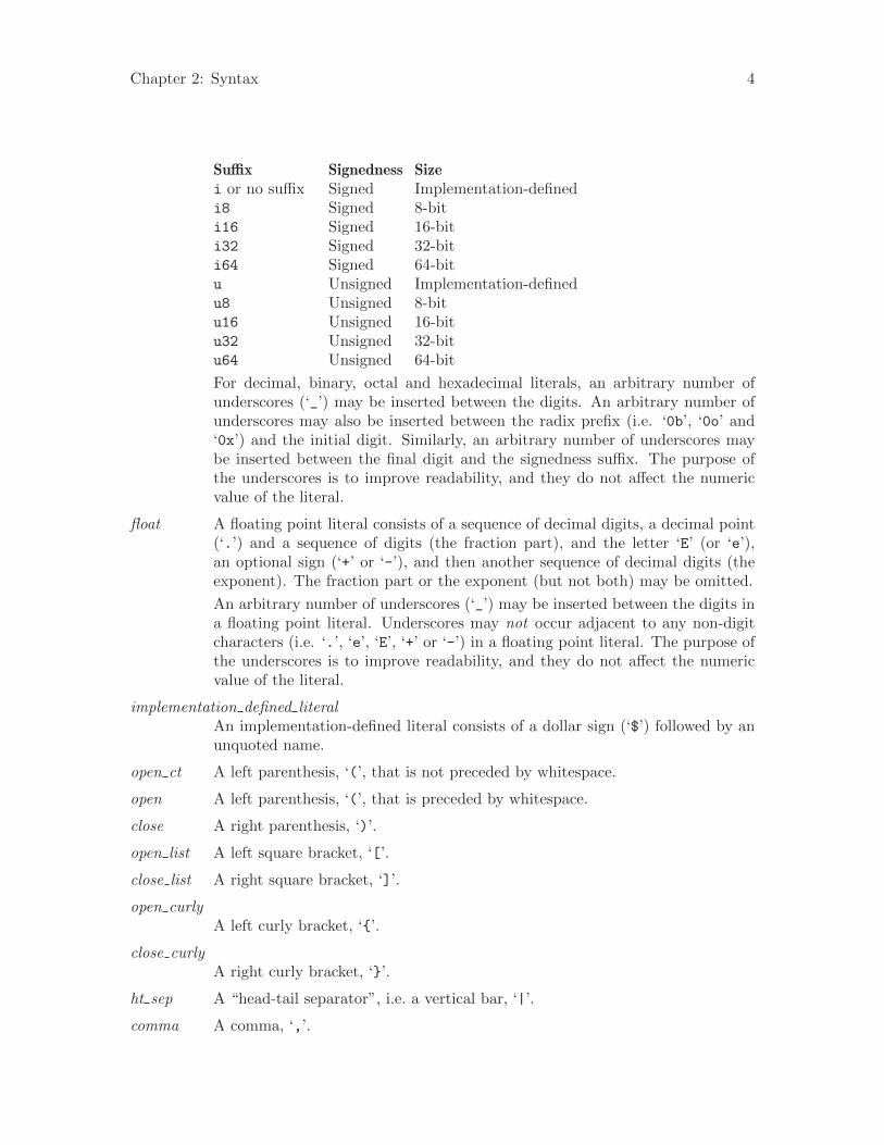
Decimal, binary, octal and hexadecimal literals may be optionally terminatedby a suffix that indicates whether the literal represents a signed or unsignedinteger and what the size of that integer is. These suffixes are:
Chapter 2: Syntax 4
Suffix Signedness Sizei or no suffix Signed Implementation-definedi8 Signed 8-biti16 Signed 16-biti32 Signed 32-biti64 Signed 64-bitu Unsigned Implementation-definedu8 Unsigned 8-bitu16 Unsigned 16-bitu32 Unsigned 32-bitu64 Unsigned 64-bit
For decimal, binary, octal and hexadecimal literals, an arbitrary number ofunderscores (‘_’) may be inserted between the digits. An arbitrary number ofunderscores may also be inserted between the radix prefix (i.e. ‘0b’, ‘0o’ and‘0x’) and the initial digit. Similarly, an arbitrary number of underscores maybe inserted between the final digit and the signedness suffix. The purpose ofthe underscores is to improve readability, and they do not affect the numericvalue of the literal.
float A floating point literal consists of a sequence of decimal digits, a decimal point(‘.’) and a sequence of digits (the fraction part), and the letter ‘E’ (or ‘e’),an optional sign (‘+’ or ‘-’), and then another sequence of decimal digits (theexponent). The fraction part or the exponent (but not both) may be omitted.
An arbitrary number of underscores (‘_’) may be inserted between the digits ina floating point literal. Underscores may not occur adjacent to any non-digitcharacters (i.e. ‘.’, ‘e’, ‘E’, ‘+’ or ‘-’) in a floating point literal. The purpose ofthe underscores is to improve readability, and they do not affect the numericvalue of the literal.
implementation defined literalAn implementation-defined literal consists of a dollar sign (‘$’) followed by anunquoted name.
open ct A left parenthesis, ‘(’, that is not preceded by whitespace.
open A left parenthesis, ‘(’, that is preceded by whitespace.
close A right parenthesis, ‘)’.
open list A left square bracket, ‘[’.
close list A right square bracket, ‘]’.
open curlyA left curly bracket, ‘{’.
close curlyA right curly bracket, ‘}’.
ht sep A “head-tail separator”, i.e. a vertical bar, ‘|’.
comma A comma, ‘,’.
Chapter 2: Syntax 5
end A full stop (period), ‘.’.
eof The end of file.
2.5 Terms
A term is either a variable or a functor.
A functor is an integer, a float, a string, a name, a compound term, or a higher-orderterm.
A compound term is a simple compound term, a list term, a tuple term, an operatorterm, or a parenthesized term.
A simple compound term is a name followed without any intervening whitespace byan open parenthesis (i.e. an open ct token), a sequence of argument terms separated bycommas, and a close parenthesis.
A list term is an open square bracket (i.e. an open list token) followed by a sequence ofargument terms separated by commas, optionally followed by a vertical bar (i.e. a ht septoken) followed by a term, followed by a close square bracket (i.e. a close list token). Anempty list term is an open list token followed by a close list token. List terms are parsedas follows:
parse(’[’ ’]’) = [].
parse(’[’ List) = parse_list(List).
parse_list(Head ’,’ Tail) = ’[|]’(parse_term(Head), parse_list(Tail)).
parse_list(Head ’|’ Tail ’]’) = ’[|]’(parse_term(Head), parse_term(Tail)).
parse_list(Head ’]’) = ’[|]’(parse_term(Head), []).
The following terms are all equivalent:
[1, 2, 3]
[1, 2, 3 | []]
[1, 2 | [3]]
[1 | [2, 3]]
’[|]’(1, ’[|]’(2, ’[|]’(3, [])))
A tuple term is a left curly bracket (i.e. an open curly token) followed by a sequence ofargument terms separated by commas, and a right curly bracket. For example, {1, ’2’,
"three"} is a valid tuple term.
An operator term is a term specified using operator notation, as in Prolog. Operatorscan also be formed by enclosing a name, a module qualified name (see Section 9.1 [Themodule system], page 66), or a variable between grave accents (backquotes). Any name orvariable may be used as an operator in this way. If fun is a variable or name, then a term ofthe form X ‘fun‘ Y is equivalent to fun(X, Y). The operator is left associative and bindsmore tightly than every operator other than ‘^’ (see Section 2.6 [Builtin operators], page 6).
A parenthesized term is just an open parenthesis followed by a term and a close paren-thesis.
A higher-order term is a “closure” term, which can be any term other than a nameor an operator term, followed without any intervening whitespace by an open parenthesis(i.e. an open ct token), a sequence of argument terms separated by commas, and a closeparenthesis. A higher-order term is equivalent to a simple compound term whose functor

Chapter 2: Syntax 6
is the empty name, and whose arguments are the closure term followed by the argumentterms of the higher-order term. That is, a term such as Term(Arg1, ..., ArgN) is parsed as’’(Term, Arg1, ..., ArgN). Note that the closure term can be a parenthesized term; forexample, (Term ^ FieldName)(Arg1, Arg2) is a higher-order term, and so it gets parsedas if it were ’’((Term ^ FieldName), Arg1, Arg2).
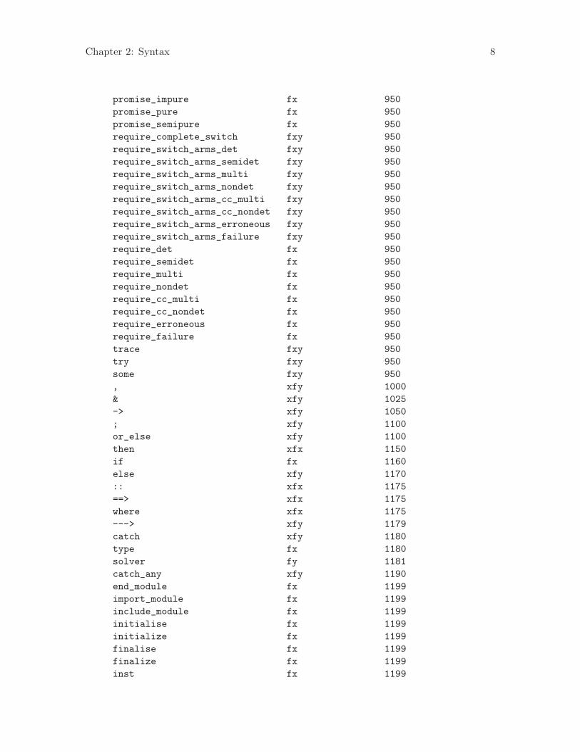
2.6 Builtin operators
The following table lists all of Mercury’s builtin operators. Operators with a low “Priority”bind more tightly than those with a high “Priority”. For example, given that + has priority500 and * has priority 400, the term 2 * X + Y would parse as (2 * X) + Y.
The “Specifier” field indicates what structure terms constructed with an operator areallowed to take. “f” represents the operator and “x” and “y” represent arguments. “x”represents an argument whose priority must be strictly lower than that of the operator. “y”represents an argument whose priority is lower or equal to that of the operator. For example,“yfx” indicates a left-associative infix operator, while “xfy” indicates a right-associative infixoperator.
Operator Specifier Priority
. yfx 10
! fx 40
!. fx 40
!: fx 40
@ xfx 90
^ xfy 99
^ fx 100
event fx 100
: yfx 120
‘op‘ yfx 120 1
** xfy 200
- fx 200
\ fx 200
* yfx 400
/ yfx 400
// yfx 400
<< yfx 400
>> yfx 400
div yfx 400
mod xfx 400
rem xfx 400
for xfx 500
+ fx 500
+ yfx 500
++ xfy 500
1 Operator term (see Section 2.5 [Terms], page 5).

Chapter 2: Syntax 7
- yfx 500
-- yfx 500
/\ yfx 500
\/ yfx 500
.. xfx 550
:= xfx 650
=^ xfx 650
< xfx 700
= xfx 700
=.. xfx 700
=:= xfx 700
=< xfx 700
== xfx 700
=\= xfx 700
> xfx 700
>= xfx 700
@< xfx 700
@=< xfx 700
@> xfx 700
@>= xfx 700
\= xfx 700
\== xfx 700
~= xfx 700
is xfx 701
and xfy 720
or xfy 740
func fx 800
impure fy 800
pred fx 800
semipure fy 800
\+ fy 900
not fy 900
when xfx 900
~ fy 900
<= xfy 920
<=> xfy 920
=> xfy 920
all fxy 950
arbitrary fxy 950
atomic fxy 950
disable_warning fxy 950
disable_warnings fxy 950
promise_equivalent_solutions fxy 950
promise_equivalent_solution_sets fxy 950
promise_exclusive fy 950
promise_exclusive_exhaustive fy 950
promise_exhaustive fy 950
Chapter 2: Syntax 8
promise_impure fx 950
promise_pure fx 950
promise_semipure fx 950
require_complete_switch fxy 950
require_switch_arms_det fxy 950
require_switch_arms_semidet fxy 950
require_switch_arms_multi fxy 950
require_switch_arms_nondet fxy 950
require_switch_arms_cc_multi fxy 950
require_switch_arms_cc_nondet fxy 950
require_switch_arms_erroneous fxy 950
require_switch_arms_failure fxy 950
require_det fx 950
require_semidet fx 950
require_multi fx 950
require_nondet fx 950
require_cc_multi fx 950
require_cc_nondet fx 950
require_erroneous fx 950
require_failure fx 950
trace fxy 950
try fxy 950
some fxy 950
, xfy 1000
& xfy 1025
-> xfy 1050
; xfy 1100
or_else xfy 1100
then xfx 1150
if fx 1160
else xfy 1170
:: xfx 1175
==> xfx 1175
where xfx 1175
---> xfy 1179
catch xfy 1180
type fx 1180
solver fy 1181
catch_any xfy 1190
end_module fx 1199
import_module fx 1199
include_module fx 1199
initialise fx 1199
initialize fx 1199
finalise fx 1199
finalize fx 1199
inst fx 1199

Chapter 2: Syntax 9
instance fx 1199
mode fx 1199
module fx 1199
pragma fx 1199
promise fx 1199
rule fx 1199
typeclass fx 1199
use_module fx 1199
--> xfx 1200
:- fx 1200
:- xfx 1200
?- fx 1200
2.7 Items
Each item in a Mercury module is either a declaration or a clause. If the top-level functorof the term is ‘:-/1’, the item is a declaration, otherwise it is a clause. There are threetypes of clauses. If the top-level functor of the item is ‘:-/2’, the item is a rule. If thetop-level functor is ‘-->/2’, the item is a DCG rule. Otherwise, the item is a fact. Thereare two types of rules and facts. If the top-level functor of the head of a rule is ‘=/2’, therule is a function rule, otherwise it is a predicate rule. If the top-level functor of the headof a fact is ‘=/2’, the fact is a function fact, otherwise it is a predicate fact.
2.8 Declarations
The allowed declarations are:
:- type
:- solver type
:- pred
:- func
:- inst
:- mode
:- typeclass
:- instance
:- pragma
:- promise
:- initialise
:- finalise
:- mutable
:- module
:- interface
:- implementation
:- import_module
:- use_module
:- include_module
:- end_module

Chapter 2: Syntax 10
The ‘type’, ‘solver type’, ‘pred’, ‘func’, ‘typeclass’ and ‘instance’ declarations areused for the type system, the ‘inst’ and ‘mode’ declarations are for the mode system, the‘pragma’ declarations are for the foreign language interface, and for compiler hints aboutinlining, and the remainder are for the module system. They are described in more detailin their respective chapters.
2.9 Facts
A function fact is an item of the form ‘Head = Result ’. A predicate fact is an item of theform ‘Head ’, where the top-level functor of Head is not :-/1, :-/2, -->/2, or =/2. In bothcases, the Head term must not be a variable. The top-level functor of the Head determineswhich predicate or function the fact belongs to; the predicate or function must have beendeclared in a preceding ‘pred’ or ‘func’ declaration in this module. The Result (if any) andthe arguments of the Head must be valid data-terms (optionally annotated with a modequalifier; see Section 4.4 [Different clauses for different modes], page 44).
A fact is equivalent to a rule whose body is ‘true’.
2.10 Rules
A function rule is an item of the form ‘Head = Result :- Body ’. A predicate rule is anitem of the form ‘Head :- Body ’ where the top-level functor of ‘Head’ is not =/2. In bothcases, the Head term must not be a variable. The top-level functor of the Head determineswhich predicate or function the clause belongs to; the predicate or function must havebeen declared in a preceding ‘pred’ or ‘func’ declaration in this module. The Result andthe arguments of the Head must be valid data-terms (optionally annotated with a modequalifier; see Section 4.4 [Different clauses for different modes], page 44). The Body mustbe a valid goal.
2.11 Goals
A goal is a term of one of the following forms:
some Vars Goal
An existential quantification. Vars must be a list of variables. Goal must be avalid goal.
Each existential quantification introduces a new scope. The variables in Varsare local to the goal Goal: for each variable named in Vars, any occurrences ofvariables with that name in Goal are considered to name a different variablethan any variables with the same name that occur outside of the existentialquantification.
Operationally, existential quantification has no effect, so apart from its effecton variable scoping, ‘some Vars Goal ’ is the same as ‘Goal ’.
Mercury’s rules for implicit quantification (see Section 2.17 [Implicit quantifica-tion], page 26) mean that variables are often implicitly existentially quantified.There is usually no need to write existential quantifiers explicitly.
all Vars Goal
A universal quantification. Vars must be a list of variables. Goal must be avalid goal. This is an abbreviation for ‘not (some Vars not Goal)’.

Chapter 2: Syntax 11
Goal1, Goal2
A conjunction. Goal1 and Goal2 must be valid goals.
Goal1 & Goal2
A parallel conjunction. This has the same declarative semantics as the normalconjunction. Operationally, implementations may execute Goal1 & Goal2 inparallel. The order in which parallel conjuncts begin execution is not fixed. It isan error for Goal1 or Goal2 to have a determinism other than det or cc_multi.See Section 6.1 [Determinism categories], page 48.
Goal1 ; Goal2
where Goal1 is not of the form ‘Goal1a -> Goal1b ’: a disjunction. Goal1 andGoal2 must be valid goals.
true The empty conjunction. Always succeeds.
fail The empty disjunction. Always fails.
not Goal
\+ Goal A negation. The two different syntaxes have identical semantics. Goal must bea valid goal. Both forms are equivalent to ‘if Goal then fail else true’.
Goal1 => Goal2
An implication. This is an abbreviation for ‘not (Goal1, not Goal2)’.
Goal1 <= Goal2
A reverse implication. This is an abbreviation for ‘not (Goal2, not Goal1)’.
Goal1 <=> Goal2
A logical equivalence. This is an abbreviation for ‘(Goal1 => Goal2), (Goal1
<= Goal2 ’).
if CondGoal then ThenGoal else ElseGoal
CondGoal -> ThenGoal ; ElseGoal
An if-then-else. The two different syntaxes have identical semantics. CondGoal,ThenGoal, and ElseGoal must be valid goals. Note that the “else” part is notoptional.
The declarative semantics of an if-then-else is given by ( CondGoal, ThenGoal
; not(CondGoal), ElseGoal), but the operational semantics are different, andit is treated differently for the purposes of determinism inference (see Chapter 6[Determinism], page 48). Operationally, it executes the CondGoal, and if thatsucceeds, then execution continues with the ThenGoal; otherwise, i.e. if Cond-Goal fails, it executes the ElseGoal. Note that CondGoal can be nondeter-ministic — unlike Prolog, Mercury’s if-then-else does not commit to the firstsolution of the condition if the condition succeeds.
If CondGoal is an explicit existential quantification, some Vars Quantified-
CondGoal , then the variables Vars are existentially quantified over the con-junction of the goals QuantifiedCondGoal and ThenGoal. Explicit existentialquantifications that occur as subgoals of CondGoal do not affect the scope ofvariables in the “then” part. For example, in
( if some [V] C then T else E )

Chapter 2: Syntax 12
the variable V is quantified over the conjunction of the goals C and T becausethe top-level goal of the condition is an explicit existential quantification, butin
( if true, some [V] C then T else E )
the variable V is only quantified over C because the top-level goal of the con-dition is not an explicit existential quantification.
Term1 = Term2
A unification. Term1 and Term2 must be valid data-terms.
Term1 \= Term2
An inequality. Term1 and Term2 must be valid data-terms. This is an abbre-viation for ‘not (Term1 = Term2)’.
call(Closure)
call(Closure1, Arg1)
call(Closure2, Arg1, Arg2)
call(Closure3, Arg1, Arg2, Arg3)
. . . A higher-order predicate call. The closure and arguments must be valid data-terms. ‘call(Closure)’ just calls the specified closure. The other forms appendthe specified arguments onto the argument list of the closure before calling it.See Chapter 8 [Higher-order], page 59.
Var
Var(Arg1)
Var(Arg2)
Var(Arg2, Arg3)
. . . A higher-order predicate call. Var must be a variable. The semantics areexactly the same as for the corresponding higher-order call using the call/N
syntax, i.e. ‘call(Var)’, ‘call(Var, Arg1)’, etc.
promise_pure Goal
A purity cast. Goal must be a valid goal. This goal promises that Goal im-plements a pure interface, even though it may include impure and semipurecomponents.
promise_semipure Goal
A purity cast. Goal must be a valid goal. This goal promises that Goal imple-ments a semipure interface, even though it may include impure components.
promise_impure Goal
A purity cast. Goal must be a valid goal. This goal instructs the compiler totreat Goal as though it were impure, regardless of its actual purity.
promise_equivalent_solutions Vars Goal
A determinism cast. Vars must be a list of variables. Goal must be a validgoal. This goal promises that Vars is the set of variables bound by Goal, andthat while Goal may have more than one solution, all of these solutions areequivalent with respect to the equality theories of the variables in Vars. It isan error for Vars to include a variable not bound by Goal or for Goal to binda non-local variable that is not listed in Vars (non-local variables with inst any

Chapter 2: Syntax 13
are assumed to be further constrained by Goal and must also be included inVars). If Goal has determinism multi or cc_multi then promise_equivalent_
solutions Vars Goal has determinism det. If Goal has determinism nondet
or cc_nondet then promise_equivalent_solutions Vars Goal has determin-ism semidet.
promise_equivalent_solution_sets Vars Goal
A determinism cast, of the kind performed by promise_equivalent_
solutions, on any goals of the form arbitrary ArbVars ArbGoal insideGoal, of which there should be at least one. Vars and ArbVars must be lists ofvariables, and Goal and ArbGoal must be valid goals. Vars must be the set ofvariables bound by Goal, and ArbVars must be the set of variables bound byArbGoal, It is an error for Vars to include a variable not bound by Goal or forGoal to bind a non-local variable that is not listed in Vars, and similarly forArbVars and ArbGoal. The intersection of Vars and the ArbVars list of anyarbitrary ArbVars ArbGoal goal included inside Goal must be empty.
The overall promise equivalent solution sets goal promises that the set of so-lutions computed for Vars by Goal is not influenced by which of the possiblesolutions for ArbVars is computed by each ArbGoal; while different choices ofsolutions for some of the ArbGoals may lead to syntactically different solutionsfor Vars for Goal, all of these solutions are equivalent with respect to the equal-ity theories of the variables in Vars. If an ArbGoal has determinism multi orcc_multi then arbitrary ArbVars ArbGoal has determinism det. If ArbGoalhas determinism nondet or cc_nondet then arbitrary ArbVars ArbGoal hasdeterminism semidet. Goal itself may have any determinism.
There is no requirement that given one of the ArbGoals, all its solutions must beequivalent with respect to the equality theories of the corresponding ArbVars;in fact, in typical usage, this won’t be the case. The different solutions of thenested arbitrary goals are not required to be equivalent in any context exceptthe promise equivalent solution sets goal they are nested inside.
Goals of the form arbitrary ArbVars ArbGoal are not allowed to occur outsidepromise_equivalent_solution_sets Vars Goal goals.
require_det Goal
require_semidet Goal
require_multi Goal
require_nondet Goal
require_cc_multi Goal
require_cc_nondet Goal
require_erroneous Goal
require_failure Goal
A determinism check, typically used to enhance the robustness of code. Goalmust be a valid goal. If Goal is det, then require_det Goal is equivalent tojust Goal. If Goal is not det, then the compiler is required to generate an errormessage.
The require_det keyword may be replaced with require_semidet, require_multi, require_nondet, require_cc_multi, require_cc_nondet, require_
Chapter 2: Syntax 14
erroneous or require_failure, each of which requires Goal to have the nameddeterminism.
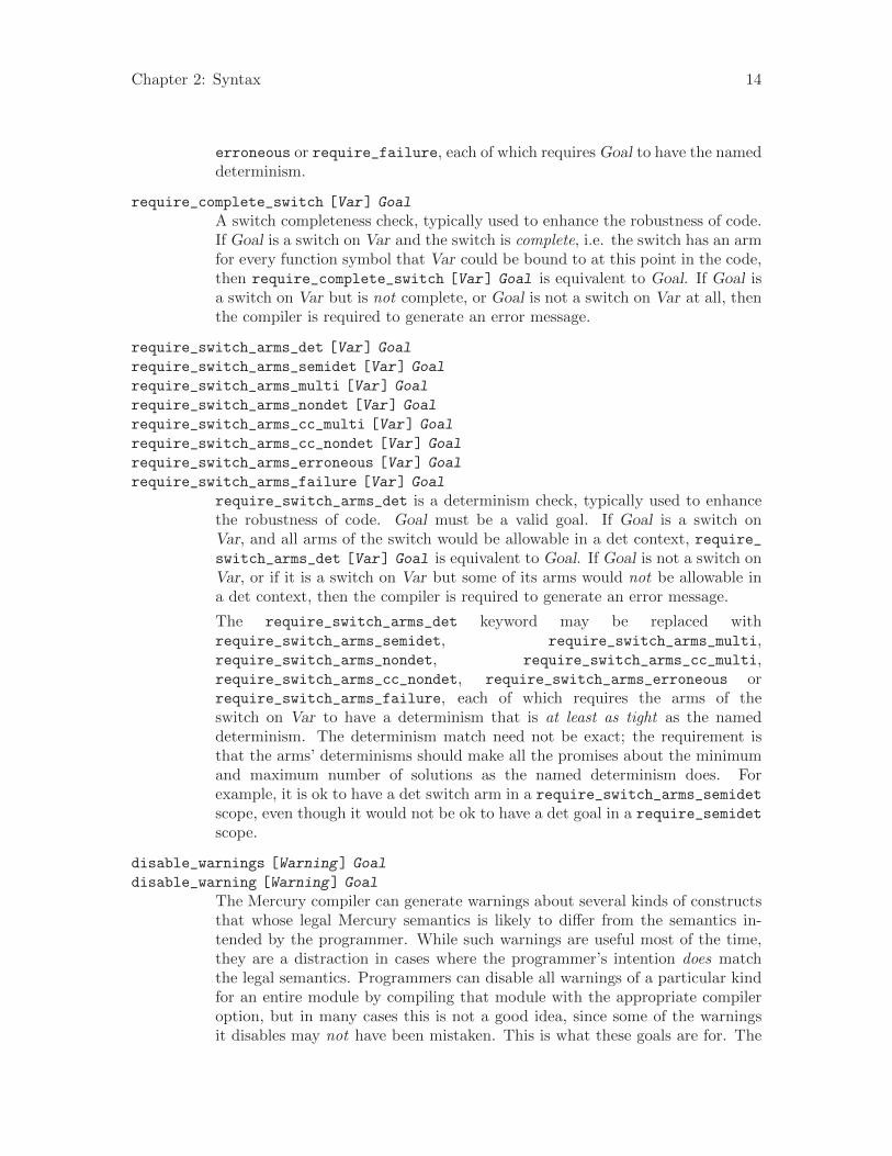
require_complete_switch [Var] Goal
A switch completeness check, typically used to enhance the robustness of code.If Goal is a switch on Var and the switch is complete, i.e. the switch has an armfor every function symbol that Var could be bound to at this point in the code,then require_complete_switch [Var] Goal is equivalent to Goal. If Goal isa switch on Var but is not complete, or Goal is not a switch on Var at all, thenthe compiler is required to generate an error message.
require_switch_arms_det [Var] Goal
require_switch_arms_semidet [Var] Goal
require_switch_arms_multi [Var] Goal
require_switch_arms_nondet [Var] Goal
require_switch_arms_cc_multi [Var] Goal
require_switch_arms_cc_nondet [Var] Goal
require_switch_arms_erroneous [Var] Goal
require_switch_arms_failure [Var] Goal
require_switch_arms_det is a determinism check, typically used to enhancethe robustness of code. Goal must be a valid goal. If Goal is a switch onVar, and all arms of the switch would be allowable in a det context, require_switch_arms_det [Var] Goal is equivalent to Goal. If Goal is not a switch onVar, or if it is a switch on Var but some of its arms would not be allowable ina det context, then the compiler is required to generate an error message.
The require_switch_arms_det keyword may be replaced withrequire_switch_arms_semidet, require_switch_arms_multi,require_switch_arms_nondet, require_switch_arms_cc_multi,require_switch_arms_cc_nondet, require_switch_arms_erroneous orrequire_switch_arms_failure, each of which requires the arms of theswitch on Var to have a determinism that is at least as tight as the nameddeterminism. The determinism match need not be exact; the requirement isthat the arms’ determinisms should make all the promises about the minimumand maximum number of solutions as the named determinism does. Forexample, it is ok to have a det switch arm in a require_switch_arms_semidetscope, even though it would not be ok to have a det goal in a require_semidetscope.
disable_warnings [Warning] Goal
disable_warning [Warning] Goal
The Mercury compiler can generate warnings about several kinds of constructsthat whose legal Mercury semantics is likely to differ from the semantics in-tended by the programmer. While such warnings are useful most of the time,they are a distraction in cases where the programmer’s intention does matchthe legal semantics. Programmers can disable all warnings of a particular kindfor an entire module by compiling that module with the appropriate compileroption, but in many cases this is not a good idea, since some of the warningsit disables may not have been mistaken. This is what these goals are for. The

Chapter 2: Syntax 15
goal disable_warnings [Warning] Goal is equivalent to Goal in all respects,with one exception: the Mercury compiler will not generate warnings of any ofthe categories whose names appear in [Warning].
At the moment, the Mercury compiler supports the disabling of the followingwarning categories:
singleton_vars
Disable the generation of singleton variable warnings.
suspected_occurs_check_failure
Disable the generation of warnings about code that looks like itunifies a variable with a term that contains that same variable.
suspicious_recursion
Disable the generation of warnings about suspicious recursive calls.
The keyword starting this scope may be written either as disable_warnings oras disable_warning. This is intended to make the code read more naturallyregardless of whether the list contains the name of more than one disabledwarning category.
trace Params Goal
A trace goal, typically used for debugging or logging. Goal must be a valid goal;Params must be a valid list of trace parameters. Some trace parameters specifycompile time or run time conditions; if any of these conditions are false, Goalwill not be executed. Since in some program invocations Goal may be replacedby ‘true’ in this way, Goal may not bind or change the instantiation state ofany variables it shares with the surrounding context. The things it may doare thus restricted to side effects; good programming style requires these sideeffects to not have any affect on the execution of the program itself, but to beconfined to the provision of extra information for the user of the program. SeeChapter 17 [Trace goals], page 138 for the details.
try Params Goal ... catch Term -> CGoal ...
A try goal. Exceptions thrown during the execution of Goal may be caughtand handled. A summary of the try goal syntax is:
try Params Goal
then ThenGoal
else ElseGoal
catch Term -> CatchGoal
...
catch_any CatchAnyVar -> CatchAnyGoal
See Chapter 12 [Exception handling], page 92 for the full details.
event Goal
An event goal. Goal must be a predicate call. Event goals are an extensionused by the Melbourne Mercury implementation to support user defined eventsin the Mercury debugger, ‘mdb’. See the “Debugging” chapter of the MercuryUser’s Guide for further details.

Chapter 2: Syntax 16
Call Any goal which does not match any of the above forms must be a predicate call.The top-level functor of the term determines the predicate called; the predicatemust be declared in a pred declaration in the module or in the interface of animported module. The arguments must be valid data-terms.
2.12 State variables
Clauses may use ‘state variables’ as a shorthand for naming intermediate values in asequence. That is, where in the plain syntax one might write
main(IO0, IO) :-
io.write_string("The answer is ", IO0, IO1),
io.write_int(calculate_answer(...), IO1, IO2),
io.nl(IO3, IO).
using state variable syntax one could write
main(!IO) :-
io.write_string("The answer is ", !IO),
io.write_int(calculate_answer(...), !IO),
io.nl(!IO).
A state variable is written ‘!.X ’ or ‘!:X ’, denoting the “current” or “next” value of thesequence labelled X. An argument ‘!X ’ is shorthand for two state variable arguments ‘!.X,!:X ’; that is, ‘p(..., !X, ...)’ is parsed as ‘p(..., !.X, !:X, ...)’.
Within each clause, a transformation converts state variables into sequences of ordinarylogic variables. The syntactic conversion is described in terms of the notional ‘transform’function defined next.
The transformation is applied once for each state variable X with some fresh variableswhich we shall call ThisX and NextX.
The expression ‘substitute(Term, X, ThisX, NextX)’ stands for a copy of Term withfree occurrences of ‘!.X ’ replaced with ThisX and free occurrences of ‘!:X ’ replaced withNextX (a free occurrence is one not bound by the head of a clause or lambda, or by explicitquantification.)
State variables obey special scope rules. A state variable X must be explicitly introducedeither in the head of the clause or lambda (in which case it may appear as either or bothof ‘!.X ’ or ‘!:X ’) or in an explicit quantification (in which case it must appear as ‘!X ’.) Astate variable X in the enclosing scope of a lambda or if-then-else expression may only bereferred to as ‘!.X ’ (unless the enclosing X is masked by a more local state variable of thesame name.)
For instance, the following clause employing a lambda expression
p(A, B, !S) :-
F = (pred(C::in, D::out) is det :-
q(C, D, !S)
),
( F(A, E) ->
B = E
;
B = A

Chapter 2: Syntax 17
).
is illegal because it implicitly refers to ‘!:S ’ inside the lambda expression. However
p(A, B, !S) :-
F = (pred(C::in, D::out, !.S::in, !:S::out) is det :-
q(C, D, !S)
),
( F(A, E, !S) ->
B = E
;
B = A
).
is acceptable because the state variable S accessed inside the lambda expression is locallyscoped to the lambda expression (shadowing the state variable of the same name outsidethe lambda expression), and the lambda expression may refer to the next version of a localstate variable.
There are three restrictions concerning state variables in lambdas: first, ‘!X ’ is not alegitimate function result, since it stands for two arguments, rather than one; second, ‘!X ’may not appear as a parameter term in the head of a lambda, since there is no syntaxfor specifying the modes of the two implied parameters; third, ‘!X ’ may not appear asan argument in a function application since this would not make sense given the usualinterpretation of state variables and functions.
Head :- Body
transform((Head :- Body), X, ThisX, NextX) =
substitute(Head, X, ThisX, NextX) :- transform(Body, X, ThisX, NextX)
Head --> Body
transform((Head --> Body), X, ThisX, NextX) =
substitute(Head, X, ThisX, NextX) :- transform(Body, X, ThisX, NextX)
Goal1, Goal2
transform((Goal1, Goal2), X, ThisX, NextX) =
transform(Goal1, X, ThisX, TmpX), transform(Goal2, X, TmpX, NextX)
for some fresh variable TmpX.
Goal1 ; Goal2
transform((Goal1 ; Goal2), X, ThisX, NextX) =
transform(Goal1, X, ThisX, NextX) ; transform(Goal2, X, ThisX, NextX)
not Goal
\+ Goal
transform((not Goal), X, ThisX, NextX) =
not transform(Goal1, X, ThisX, DummyX), NextX = ThisX
for some fresh variable DummyX.
if Goal1 then Goal2 else Goal3
Goal1 -> Goal2 ; Goal3
transform((if Goal1 then Goal2 else Goal3), X, ThisX, NextX) =
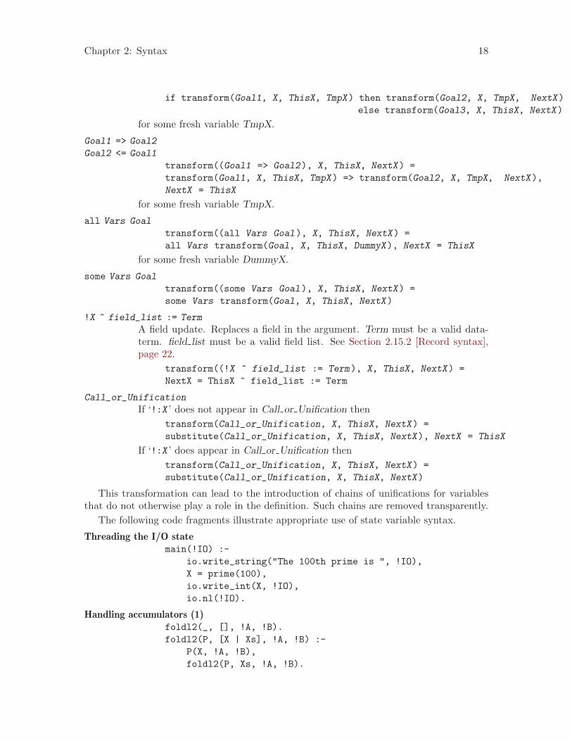
Chapter 2: Syntax 18
if transform(Goal1, X, ThisX, TmpX) then transform(Goal2, X, TmpX, NextX)
else transform(Goal3, X, ThisX, NextX)
for some fresh variable TmpX.
Goal1 => Goal2
Goal2 <= Goal1
transform((Goal1 => Goal2), X, ThisX, NextX) =
transform(Goal1, X, ThisX, TmpX) => transform(Goal2, X, TmpX, NextX),
NextX = ThisX
for some fresh variable TmpX.
all Vars Goal
transform((all Vars Goal), X, ThisX, NextX) =
all Vars transform(Goal, X, ThisX, DummyX), NextX = ThisX
for some fresh variable DummyX.
some Vars Goal
transform((some Vars Goal), X, ThisX, NextX) =
some Vars transform(Goal, X, ThisX, NextX)
!X ^ field_list := Term
A field update. Replaces a field in the argument. Term must be a valid data-term. field list must be a valid field list. See Section 2.15.2 [Record syntax],page 22.
transform((!X ^ field_list := Term), X, ThisX, NextX) =
NextX = ThisX ^ field_list := Term
Call_or_Unification
If ‘!:X ’ does not appear in Call or Unification then
transform(Call_or_Unification, X, ThisX, NextX) =
substitute(Call_or_Unification, X, ThisX, NextX), NextX = ThisX
If ‘!:X ’ does appear in Call or Unification then
transform(Call_or_Unification, X, ThisX, NextX) =
substitute(Call_or_Unification, X, ThisX, NextX)
This transformation can lead to the introduction of chains of unifications for variablesthat do not otherwise play a role in the definition. Such chains are removed transparently.
The following code fragments illustrate appropriate use of state variable syntax.
Threading the I/O statemain(!IO) :-
io.write_string("The 100th prime is ", !IO),
X = prime(100),
io.write_int(X, !IO),
io.nl(!IO).
Handling accumulators (1)foldl2(_, [], !A, !B).
foldl2(P, [X | Xs], !A, !B) :-
P(X, !A, !B),
foldl2(P, Xs, !A, !B).

Chapter 2: Syntax 19
Handling accumulators (2)iterate_while2(P, F, !A, !B) :-
( if P(!.A, !.B) then
F(!A, !B),
iterate_while2(P, F, !A, !B)
else
true
).
2.13 DCG-rules
Definite Clause Grammar notation is intended for writing parsers and sequence generatorsin a particular style; in the past it has also been used to thread an implicit state variable,typically the I/O state, through code. As a matter of style, we recommend that in futureDCG notation be reserved for writing parsers and sequence generators, and that statevariable syntax be used for passing state threads.
DCG-rules in Mercury have identical syntax and semantics to DCG-rules in Prolog.
A DCG-rule is an item of the form ‘Head --> Body ’. The Head term must not be a vari-able. A DCG-rule is an abbreviation for an ordinary rule with two additional implicit argu-ments appended to the arguments of Head. These arguments are fresh variables, which weshall call V in and V out. The Body must be a valid DCG-goal, and is an abbreviation foran ordinary goal. The next section defines a mathematical function ‘DCG-transform(V_in,V_out, DCG-goal)’ which specifies the semantics of how DCG goals are transformed intoordinary goals. (The ‘DCG-transform’ function is purely for the purposes of exposition, todefine the semantics — it is not part of the language.)
2.14 DCG-goals
A DCG-goal is a term of one of the following forms:
some Vars DCG-goal
A DCG existential quantification. Vars must be a list of variables. DCG-goalmust be a valid DCG-goal.
Semantics:
transform(V_in, V_out, some Vars DCG_goal) =
some Vars transform(V_in, V_out, DCG_goal)
all Vars DCG-goal
A DCG universal quantification. Vars must be a list of variables. DCG-goalmust be a valid DCG-goal.
Semantics:
transform(V_in, V_out, all Vars DCG_goal) =
all Vars transform(V_in, V_out, DCG_goal)
DCG-goal1, DCG-goal2
A DCG sequence. Intuitively, this means “parse DCG-goal1 and then parseDCG-goal2” or “do DCG-goal1 and then do DCG-goal2”. (Note that the onlyway this construct actually forces the desired sequencing is by the modes of the
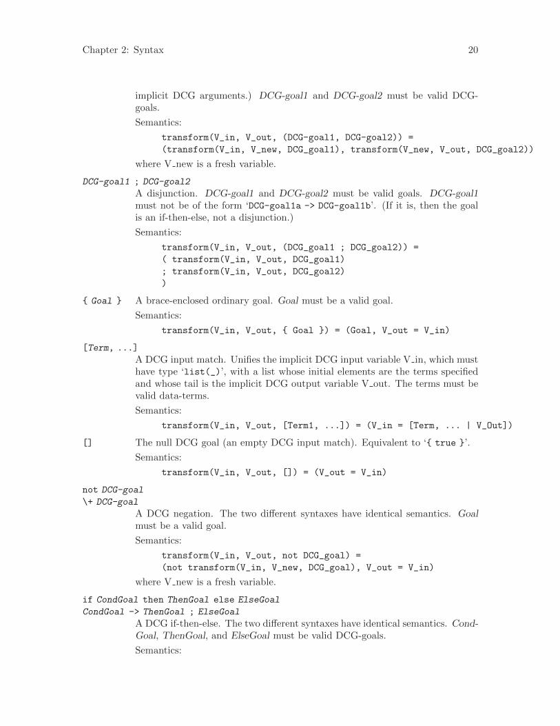
Chapter 2: Syntax 20
implicit DCG arguments.) DCG-goal1 and DCG-goal2 must be valid DCG-goals.
Semantics:
transform(V_in, V_out, (DCG-goal1, DCG-goal2)) =
(transform(V_in, V_new, DCG_goal1), transform(V_new, V_out, DCG_goal2))
where V new is a fresh variable.
DCG-goal1 ; DCG-goal2
A disjunction. DCG-goal1 and DCG-goal2 must be valid goals. DCG-goal1must not be of the form ‘DCG-goal1a -> DCG-goal1b’. (If it is, then the goalis an if-then-else, not a disjunction.)
Semantics:
transform(V_in, V_out, (DCG_goal1 ; DCG_goal2)) =
( transform(V_in, V_out, DCG_goal1)
; transform(V_in, V_out, DCG_goal2)
)
{ Goal } A brace-enclosed ordinary goal. Goal must be a valid goal.
Semantics:
transform(V_in, V_out, { Goal }) = (Goal, V_out = V_in)
[Term, ...]
A DCG input match. Unifies the implicit DCG input variable V in, which musthave type ‘list(_)’, with a list whose initial elements are the terms specifiedand whose tail is the implicit DCG output variable V out. The terms must bevalid data-terms.
Semantics:
transform(V_in, V_out, [Term1, ...]) = (V_in = [Term, ... | V_Out])
[] The null DCG goal (an empty DCG input match). Equivalent to ‘{ true }’.
Semantics:
transform(V_in, V_out, []) = (V_out = V_in)
not DCG-goal
\+ DCG-goal
A DCG negation. The two different syntaxes have identical semantics. Goalmust be a valid goal.
Semantics:
transform(V_in, V_out, not DCG_goal) =
(not transform(V_in, V_new, DCG_goal), V_out = V_in)
where V new is a fresh variable.
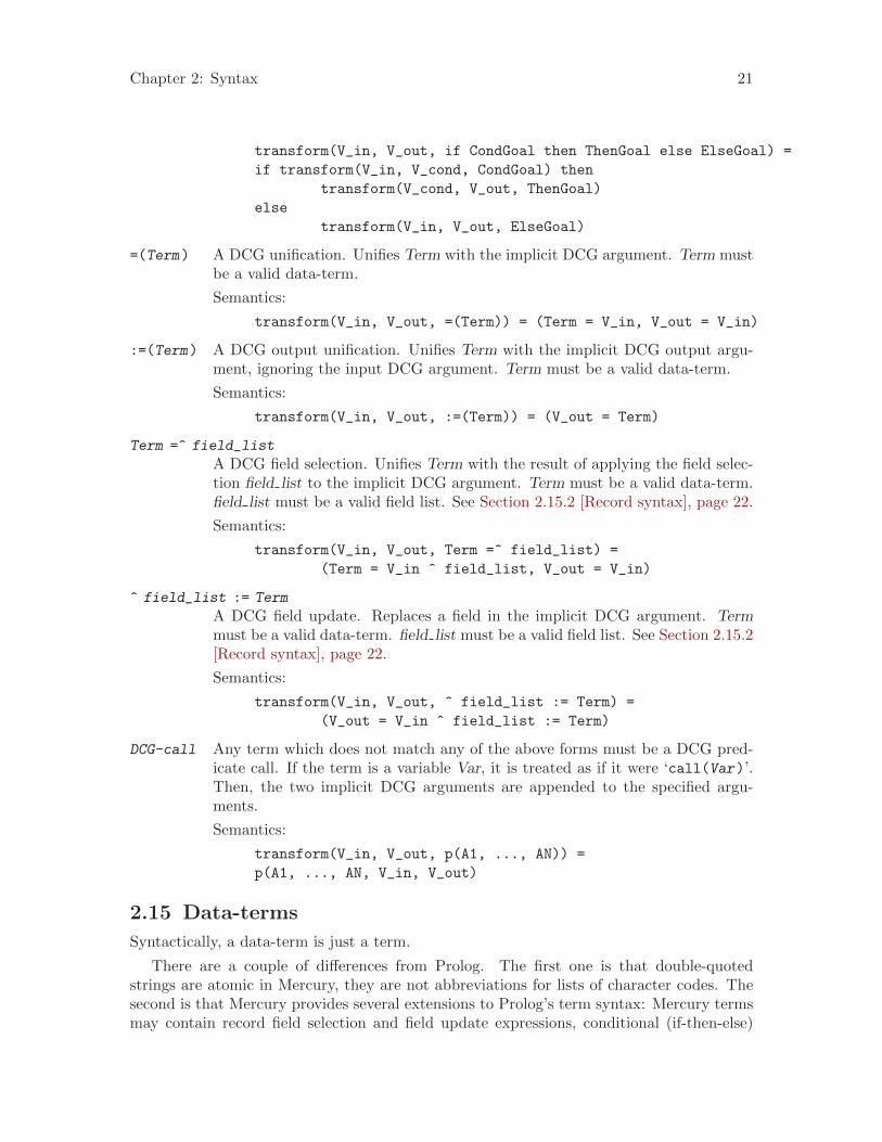
if CondGoal then ThenGoal else ElseGoal
CondGoal -> ThenGoal ; ElseGoal
A DCG if-then-else. The two different syntaxes have identical semantics. Cond-Goal, ThenGoal, and ElseGoal must be valid DCG-goals.
Semantics:
Chapter 2: Syntax 21
transform(V_in, V_out, if CondGoal then ThenGoal else ElseGoal) =
if transform(V_in, V_cond, CondGoal) then
transform(V_cond, V_out, ThenGoal)
else
transform(V_in, V_out, ElseGoal)
=(Term) A DCG unification. Unifies Term with the implicit DCG argument. Term mustbe a valid data-term.
Semantics:
transform(V_in, V_out, =(Term)) = (Term = V_in, V_out = V_in)
:=(Term) A DCG output unification. Unifies Term with the implicit DCG output argu-ment, ignoring the input DCG argument. Term must be a valid data-term.
Semantics:
transform(V_in, V_out, :=(Term)) = (V_out = Term)
Term =^ field_list
A DCG field selection. Unifies Term with the result of applying the field selec-tion field list to the implicit DCG argument. Term must be a valid data-term.field list must be a valid field list. See Section 2.15.2 [Record syntax], page 22.
Semantics:
transform(V_in, V_out, Term =^ field_list) =
(Term = V_in ^ field_list, V_out = V_in)
^ field_list := Term
A DCG field update. Replaces a field in the implicit DCG argument. Termmust be a valid data-term. field list must be a valid field list. See Section 2.15.2[Record syntax], page 22.
Semantics:
transform(V_in, V_out, ^ field_list := Term) =
(V_out = V_in ^ field_list := Term)
DCG-call Any term which does not match any of the above forms must be a DCG pred-icate call. If the term is a variable Var, it is treated as if it were ‘call(Var)’.Then, the two implicit DCG arguments are appended to the specified argu-ments.
Semantics:
transform(V_in, V_out, p(A1, ..., AN)) =
p(A1, ..., AN, V_in, V_out)
2.15 Data-terms
Syntactically, a data-term is just a term.
There are a couple of differences from Prolog. The first one is that double-quotedstrings are atomic in Mercury, they are not abbreviations for lists of character codes. Thesecond is that Mercury provides several extensions to Prolog’s term syntax: Mercury termsmay contain record field selection and field update expressions, conditional (if-then-else)

Chapter 2: Syntax 22
expressions, function applications, higher-order function applications, lambda expressions,and explicit type qualifications.
A data-term is either a variable, a data-functor, or a special data-term. A special data-term is a conditional expression, a record syntax expression, a unification expression, alambda expression, a higher-order function application, or an explicit type qualification.
2.15.1 Data-functors
A data-functor is an integer, a float, a string, a character literal (any single-charactername), a name, an implementation-defined literal, or a compound data-term. A compounddata-term is a compound term which does not match the form of a special data-term (seeSection 2.15 [Data-terms], page 21), and whose arguments are data-terms. If a data-functoris a name or a compound data-term, its top-level functor must name a function, predicate,or data constructor declared in the module or in the interface of an imported module.
Implementation-defined literals are symbolic names whose value represents a propertyof the compilation environment or the context in which it appears. The implementationreplaces these symbolic names with actual constants during compilation. Implementation-defined literals can only appear within clauses. The following literals must be supported byall Mercury implementations:
‘$file’ a string that gives the name of the file that contains the module being compiled.If the name of the file cannot be determined, then it is replaced by an arbitrarystring.
‘$line’ the line number (integer) of the goal in which the literal appears, or -1 if itcannot be determined.
‘$module’ a string representation of the fully qualified module name.
‘$pred’ a string containing the fully qualified predicate or function name and arity.
The Melbourne Mercury implementation additionally supports the following extension:
‘$grade’ the grade (string) in which the module is compiled.
2.15.2 Record syntax
Record syntax provides a convenient way to select or update fields of data constructors,independent of the definition of the constructor. Record syntax expressions are transformedinto sequences of calls to field selection or update functions (see Section 3.4 [Field accessfunctions], page 34).
A field specifier is a name or a compound data-term. A field list is a list of field specifiersseparated by ^. field, field1 ^ field2 and field1(A) ^ field2(B, C) are all valid fieldlists.
If the top-level functor of a field specifier is ‘field/N’, there must be a visible selectionfunction ‘field/(N + 1)’. If the field specifier occurs in a field update expression, theremust also be a visible update function named ‘’field :=’/(N + 2)’.
Record syntax expressions have one of the following forms. There are also record syntaxDCG goals (see Section 2.14 [DCG-goals], page 19), which provide similar functionality torecord syntax expressions, except that they act on the DCG arguments of a DCG clause.

Chapter 2: Syntax 23
Term ^ field_list
A field selection. For each field specifier in field list, apply the correspondingselection function in turn.
Term must be a valid data-term. field list must be a valid field list.
A field selection is transformed using the following rules:
transform(Term ^ Field(Arg1, ...)) = Field(Arg1, ..., Term).
transform(Term ^ Field(Arg1, ...) ^ Rest) =
transform(Field(Arg1, ..., Term) ^ Rest).
Examples:
Term ^ field is equivalent to field(Term).
Term ^ field(Arg) is equivalent to field(Arg, Term).
Term ^ field1(Arg1) ^ field2(Arg2, Arg3) is equivalent tofield2(Arg2, Arg3, field1(Arg1, Term)).
Term ^ field_list := FieldValue
A field update, returning a copy of Term with the value of the field specifiedby field list replaced with FieldValue.
Term must be a valid data-term. field list must be a valid field list.
A field update is transformed using the following rules:
transform(Term ^ Field(Arg1, ...) := FieldValue) =
’Field :=’(Arg1, ..., Term, FieldValue)).
transform(Term0 ^ Field(Arg1, ...) ^ Rest := FieldValue) = Term :-
OldFieldValue = Field(Arg1, ..., Term0),
NewFieldValue = transform(OldFieldValue ^ Rest := FieldValue),
Term = ’Field :=’(Arg1, ..., Term0, NewFieldValue).
Examples:
Term ^ field := FieldValue is equivalent to ’field :=’(Term, FieldValue).
Term ^ field(Arg) := FieldValue is equivalent to ’field :=’(Arg, Term, FieldValue).
Term ^ field1(Arg1) ^ field2(Arg2) := FieldValue is equivalent to thecode
OldField1 = field1(Arg1, Term),
NewField1 = ’field2 :=’(Arg2, OldField1, FieldValue),
Result = ’field1 :=’(Arg1, Term, NewField1)
2.15.3 Unification expressions
A unification expression is an expression of the form
X @ Y
where X and Y are data-terms.
The meaning of a unification expression is that the arguments are unified, and theexpression is equivalent to the unified value.
The strict sequential operational semantics (see Chapter 13 [Semantics], page 95) of anexpression X @ Y is that the expression is replaced by a fresh variable Z, and immediatelyafter Z is evaluated, the conjunction Z = X, Z = Y is evaluated.
Chapter 2: Syntax 24
For example
p(X @ f(_, _), X).
is equivalent to
p(H1, H2) :-
H1 = X,
H1 = f(_, _),
H2 = X.
Unification expressions are most useful when writing switches (see Section 6.2 [Deter-minism checking and inference], page 49). The arguments of a unification expression areexamined when checking for switches. The arguments of an equivalent user-defined functionwould not be.
2.15.4 Conditional expressions
A conditional expression is an expression of either of the two following forms
(if Goal then Expression1 else Expression2)
(Goal -> Expression1 ; Expression2)
Goal is a goal; Expression1 and Expression2 are both data-terms. The semantics of a condi-tional expression is that if Goal is true, then the expression has the meaning of Expression1,else the expression has the meaning of Expression2.
If Goal takes the form some [X, Y, Z] ... then the scope of X, Y, and Z includesExpression1.
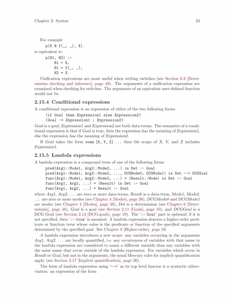
2.15.5 Lambda expressions
A lambda expression is a compound term of one of the following forms
pred(Arg1::Mode1, Arg2::Mode2, ...) is Det :- Goal
pred(Arg1::Mode1, Arg2::Mode2, ..., DCGMode0, DCGMode1) is Det --> DCGGoal
func(Arg1::Mode1, Arg2::Mode2, ...) = (Result::Mode) is Det :- Goal
func(Arg1, Arg2, ...) = (Result) is Det :- Goal
func(Arg1, Arg2, ...) = Result :- Goal
where Arg1, Arg2, . . . are zero or more data-terms, Result is a data-term, Mode1, Mode2,. . . are zero or more modes (see Chapter 4 [Modes], page 38), DCGMode0 and DCGMode1are modes (see Chapter 4 [Modes], page 38), Det is a determinism (see Chapter 6 [Deter-minism], page 48), Goal is a goal (see Section 2.11 [Goals], page 10), and DCGGoal is aDCG Goal (see Section 2.14 [DCG-goals], page 19). The ‘:- Goal’ part is optional; if it isnot specified, then ‘:- true’ is assumed. A lambda expression denotes a higher-order pred-icate or function term whose value is the predicate or function of the specified argumentsdetermined by the specified goal. See Chapter 8 [Higher-order], page 59.
A lambda expression introduces a new scope: any variables occurring in the argumentsArg1, Arg2, . . . are locally quantified, i.e. any occurrences of variables with that name inthe lambda expression are considered to name a different variable than any variables withthe same name that occur outside of the lambda expression. For variables which occur inResult or Goal, but not in the arguments, the usual Mercury rules for implicit quantificationapply (see Section 2.17 [Implicit quantification], page 26).
The form of lambda expression using ‘-->’ as its top level functor is a syntactic abbre-viation: an expression of the form

Chapter 2: Syntax 25
pred(Var1::Mode1, Var2::Mode2, ..., DCGMode0, DCGMode1) is Det --> DCGGoal
is equivalent to
pred(Var1::Mode1, Var2::Mode2, ...,
DCGVar0::DCGMode0, DCGVar1::DCGMode1) is Det :- Goal
where DCGVar0 and DCGVar1 are fresh variables, and Goal is the result of‘DCG-transform(DCGVar0, DCGVar1, DCGGoal)’ where DCG-transform is the functionspecified in Section 2.14 [DCG-goals], page 19.
2.15.6 Higher-order function applications
A higher-order function application is a compound term of one of the following two forms
apply(Func, Arg1, Arg2, ..., ArgN)
FuncVar(Arg1, Arg2, ..., ArgN)
where N >= 0, Func is a term of type ‘func(T1, T2, ..., Tn) = T’, FuncVar is a variableof that type, and Arg1, Arg2, . . . , ArgN are terms of types ‘T1’, ‘T2’, . . . , ‘Tn’. The typeof the higher-order function application term is T. It denotes the result of applying thespecified function to the specified arguments. See Chapter 8 [Higher-order], page 59.
2.15.7 Explicit type qualification
Explicit type qualifications are occasionally useful to resolve ambiguities that can arise fromoverloading or polymorphic types.
An explicit type qualification expression is a term of the form
Term : Type
Term must be a valid data-term. Type must be a valid type (see Chapter 3 [Types],page 27).
An explicit type qualification expression constrains the specified term to have the spec-ified type. Apart from that, the meaning of an explicit type qualification expression is justthe same as the specified Term.
Currently we also support the following alternative syntax for type qualification:
with_type(Term, Type)
or equivalently, as it is more commonly written,
Term ‘with_type‘ Type
2.16 Variable scoping
There are three sorts of variables in Mercury: ordinary variables, type variables, and instvariables.
Variables occurring in types are called type variables. Variables occurring in insts ormodes are called inst variables. Variables that occur in data-terms, and that are not instvariables or type variables, are called ordinary variables.
(Type variables can occur in data-terms in the right-hand [Type] operand of an explicittype qualification. Inst variables can occur in data-terms in the right-hand [Mode] operandof an explicit mode qualification. Apart from that, all other variables in data-terms areordinary variables.)
Chapter 2: Syntax 26
The three different variable sorts occupy different namespaces: there is no semanticrelationship between two variables of different sorts (e.g. a type variable and an ordinaryvariable) even if they happen to share the same name. However, as a matter of programmingstyle, it is generally a bad idea to use the same name for variables of different sorts in thesame clause.
The scope of ordinary variables is the clause or declaration in which they occur, unlessthey are quantified, either explicitly (see Section 2.11 [Goals], page 10) or implicitly (seeSection 2.17 [Implicit quantification], page 26).
The scope of type variables in a predicate or function’s type declaration extends overany explicit type qualifications (see Section 2.15.7 [Explicit type qualification], page 25) inthe clauses for that predicate or function, and over ‘pragma type_spec’ (see Section 18.2[Type specialization], page 141) declarations for that predicate or function, so that explicittype qualifications and ‘pragma type_spec’ declarations can refer to those type variables.The scope of any type variables in an explicit type qualification which do not occur in thepredicate or function’s type declaration is the clause in which they occur.
The scope of inst variables is the clause or declaration in which they occur.
2.17 Implicit quantification
The rule for implicit quantification in Mercury is not the same as the usual one in mathe-matical logic. In Mercury, variables that do not occur in the head of a clause are implicitlyexistentially quantified around their closest enclosing scope (in a sense to be made precisein the following paragraphs). This allows most existential quantifiers to be omitted, andleads to more concise code.
An occurrence of a variable is in a negated context if it is in a negation, in a universalquantification, in the condition of an if-then-else, in an inequality, or in a lambda expression.
Two goals are parallel if they are different disjuncts of the same disjunction, or if one isthe “else” part of an if-then-else and the other goal is either the “then” part or the conditionof the if-then-else, or if they are the goals of disjoint (distinct and non-overlapping) lambdaexpressions.
If a variable occurs in a negated context and does not occur outside of that negatedcontext other than in parallel goals (and in the case of a variable in the condition of anif-then-else, other than in the “then” part of the if-then-else), then that variable is implicitlyexistentially quantified inside the negation.
2.18 Elimination of double negation
The treatment of inequality, universal quantification, implication, and logical equivalenceas abbreviations can cause the introduction of double negations which could make other-wise well-formed code mode-incorrect. To avoid this problem, the language specifies thatafter syntax analysis and implicit quantification, and before mode analysis is performed, theimplementation must delete any double negations and must replace any negations of con-junctions of negations with disjunctions. (Both of these transformations preserve the logicalmeaning and type-correctness of the code, and they preserve or improve mode-correctness:they never transform code fragments that would be well-moded into ones that would beill-moded.)

Chapter 3: Types 27
3 Types
The type system is based on many-sorted logic, and supports polymorphism, type classes(see Chapter 10 [Type classes], page 74), and existentially quantified types (see Chapter 11[Existential types], page 84).
3.1 Builtin types
This section describes the special types that are built into the Mercury implementation, orare defined in the standard library.
3.1.1 Primitive types
There is a special syntax for constants of all primitive types except char. (For char, thestandard syntax suffixes.)
3.1.1.1 Signed integer types
There are five primitive signed integer types: int, int8, int16, int32 and int64.
Except for int, the width in bits of each of these is given by the numeric suffix in itsname.
The width in bits of int is implementation defined, but must be at least 32-bits.
All signed integer types use two’s-complement representation. Their width must be equalto the width of the corresponding unsigned type.
Values of the type int8 must be in the range −128 (−(28−1)) to 127 (28−1 − 1), bothinclusive.
Values of the type int16 must be in the range −32768 (−(216−1)) to 32767 (216−1 − 1),both inclusive.
Values of the type int32 must be in the range −2147483648 (−(232−1)) to 2147483647(232−1 − 1), both inclusive.
Values of the type int64 must be in the range −9223372036854775808 (−(264−1)) to9223372036854775807 (264−1 − 1), both inclusive.
Values of the type int must be in the range to −(2N−1) to 2N−1 − 1, both inclusive; Nbeing the width of int in bits.
3.1.1.2 Unsigned integer types
There are five primitive unsigned integer types: uint, uint8, uint16, uint32 and uint64.
Except for uint, the width in bits of each of these is given by the numeric suffix in itsname.
The width in bits of uint is implementation defined, but must be at least 32-bits. Itmust be equal to the width of the type int.
Values of the type uint8 must be in the range 0 (20 − 1) to 255 (28 − 1), both inclusive.
Values of the type uint16 must be in the range 0 (20 − 1) to 65535 (216 − 1), bothinclusive.
Values of the type uint32 must be in the range 0 (20 − 1) to 4294967295 (232− 1), bothinclusive.

Chapter 3: Types 28
Values of the type uint64 must be in the range 0 (20 − 1) to 18446744073709551615(264− 1), both inclusive.
Values of the type uint must be in the range 0 (20 − 1) to 2N − 1, both inclusive; Nbeing the width of uint in bits.
3.1.1.3 Floating-point type
There is one floating-point type: float.
It is represented using either the 32-bit single-precision IEEE 754 format or the 64-bitdouble-precision IEEE 754 format.
The choice between the two formats is implementation dependent.
In the Melbourne Mercury implementation, floats are represented using the 32-bitsingle-precision IEEE 754 format in grades that have .spf grade component, and using the64-bit double-precision IEEE 754 format in every other grade.
3.1.1.4 Character type
There is one character type: char.
Values of this type represent Unicode code points.
3.1.1.5 String type
There is one string type: string.
A string is a sequence of characters encoded using either the UTF-8 or UTF-16 encodingof Unicode.
The choice between the two encodings is implementation dependent.
In the Melbourne Mercury implementation, strings are represented using UTF-8 whengenerating code for C or Erlang, and using UTF-16 when generating code for C# or Java.
3.1.2 Other builtin types
3.1.2.1 Predicate and function types
The predicate types are pred, pred(T), pred(T1, T2), . . .
The function types are (func) = T, func(T1) = T, func(T1, T2) = T, . . .
Higher-order predicate and function types are used to pass closures to other predicatesand functions. See Chapter 8 [Higher-order], page 59.
3.1.2.2 Tuple types
The tuple types are {}, {T}, {T1, T2}, . . .
A tuple type is equivalent to a discriminated union type (see Section 3.2.1 [Discriminatedunions], page 29) with declaration
:- type {Arg1, Arg2, ..., ArgN}
---> { {Arg1, Arg2, ..., ArgN} }.
Chapter 3: Types 29
3.1.2.3 The universal type
The type univ is defined in the standard library module univ, along with the predicatestype_to_univ/2 and univ_to_type/2. With those predicates, values of any type can beconverted to the universal type and back again. The universal type is useful for situationswhere you need heterogeneous collections.
3.1.2.4 The “state-of-the-world” type
The type io.state is defined in the standard library module io, and represents the stateof the world. Predicates which perform I/O are passed the only reference to the currentstate of the world, and produce a unique reference to the new state of the world. In thisway, we can give a declarative semantics to code that performs I/O.
3.2 User-defined types
New types can be introduced with ‘:- type’ declarations. There are several categories ofderived types:
3.2.1 Discriminated unions
These encompass both enumeration and record types in other languages. A derived typeis defined using ‘:- type type ---> body ’. (Note there are three dashes in that arrow. Itshould not be confused with the two-dash arrow used for DCGs or the one-dash arrow usedfor if-then-else.) If the type term is a functor of arity zero (i.e. one having zero arguments),it names a monomorphic type. Otherwise, it names a polymorphic type; the argumentsof the functor must be distinct type variables. The body term is defined as a sequence ofconstructor definitions separated by semi-colons.
Ordinarily, each constructor definition must be a functor whose arguments (if any) aretypes. Ordinary discriminated union definitions must be transparent: all type variablesoccurring in the body must also occur in the type.
However, constructor definitions can optionally be existentially typed. In that case, thefunctor will be preceded by an existential type quantifier and can optionally be followed byan existential type class constraint. For details, see Chapter 11 [Existential types], page 84.Existentially typed discriminated union definitions need not be transparent.
The arguments of constructor definitions may be labelled. These labels cause the com-piler to generate functions which can be used to conveniently select and update fields of aterm in a manner independent of the definition of the type (see Section 3.4 [Field accessfunctions], page 34). A labelled argument has the form fieldname :: Type . It is an errorfor two fields in the same module to have the same label.
Here are some examples of discriminated union definitions:
:- type fruit
---> apple
; orange
; banana
; pear.
:- type strange
---> foo(int)
Chapter 3: Types 30
; bar(string).
:- type employee
---> employee(
name :: string,
age :: int,
department :: string
).
:- type tree
---> empty
; leaf(int)
; branch(tree, tree).
:- type list(T)
---> []
; [T | list(T)].
:- type pair(T1, T2)
---> T1 - T2.
If the body of a discriminated union type definition contains a term whose top-levelfunctor is ’;’/2, the semi-colon is normally assumed to be a separator. This makes itdifficult to define a type whose constructors include ’;’/2. To allow this, curly bracescan be used to quote the semi-colon. It is then also necessary to quote curly braces. Thefollowing example illustrates this:
:- type tricky
---> { int ; int }
; { { int } }.
This defines a type with two constructors, ’;’/2 and ’{}’/1, whose argument types areall int. We recommend against using constructors named ’{}’ because of the possibilityof confusion with the builtin tuple types.
Each discriminated union type definition introduces a distinct type. Mercury considerstwo discriminated union types that have the same bodies to be distinct types (name equiv-alence). Having two different definitions of a type with the same name and arity in thesame module is an error.
Constructors may be overloaded among different types: there may be any number ofconstructors with a given name and arity, so long as they all have different types. However,there must not be more than one constructor with the same name, arity, and result type inthe same module. (There is no particularly good reason for this restriction; in the futurewe may allow several such functors as long as they have different argument types.) Notethat excessive overloading of constructors can slow down type checking and can make theprogram confusing for human readers, so overloading should not be over-used.
Note that user defined types may not have names that have meanings in Mercury. (Mostof these are documented in later sections.)
The list of reserved type names is

Chapter 3: Types 31
int
int8
int16
int32
int64
uint
uint8
uint16
uint32
uint64
float
character
string
{}
=
pred
func
pure
semipure
impure
’’
3.2.2 Equivalence types
These are type abbreviations. They are defined using ‘==’ as follows. They may be poly-morphic.
:- type money == int.
:- type assoc_list(KeyType, ValueType)
== list(pair(KeyType, ValueType)).
Equivalence type definitions must be transparent. Unlike discriminated union type def-initions, equivalence type definitions must not be cyclic; that is, the type on the left handside of the ‘==’ (‘assoc_list’ and ‘money’ in the examples above) must not occur on theright hand side of the ‘==’.
Mercury treats an equivalence type as an abbreviation for the type on the right handside of the definition; the two are equivalent in all respects in scopes where the equivalencetype is visible.
3.2.3 Abstract types
These are types whose implementation is hidden. The type declarations
:- type t1.
:- type t2(T1, T2).
declare types t1/0 and t2/2 to be abstract types. Such declarations are only useful in theinterface section of a module. This means that the type names will be exported, but theconstructors (functors) for these types will not be exported. The implementation section ofa module must give a definition for all of the abstract types named in the interface sectionof the module. Abstract types may be defined as either discriminated union types or asequivalence types.

Chapter 3: Types 32
3.3 Predicate and function type declarations
The argument types of each predicate must be explicitly declared with a ‘:- pred’ decla-ration. The argument types and return type of each function must be explicitly declaredwith a ‘:- func’ declaration. For example:
:- pred is_all_uppercase(string).
:- func strlen(string) = int.
Predicates and functions can be polymorphic; that is, their declarations can include typevariables. For example:
:- pred member(T, list(T)).
:- func length(list(T)) = int.
A predicate or function can be declared to have a given higher-order type (see Chapter 8[Higher-order], page 59) by using an explicit type qualification in the type declaration. Thisis useful where several predicates or functions need to have the same type signature, whichoften occurs for type class method implementations (see Chapter 10 [Type classes], page 74),and for predicates to be passed as higher-order terms.
For example,
:- type foldl_pred(T, U) == pred(T, U, U).
:- type foldl_func(T, U) == (func(T, U) = U).
:- pred p(int) : foldl_pred(T, U).
:- func f(int) : foldl_func(T, U).
is equivalent to
:- pred p(int, T, U, U).
:- pred f(int, T, U) = U.
Type variables in predicate and function declarations are implicitly universally quantifiedby default; that is, the predicate or function may be called with arguments and (in the caseof functions) return value whose actual types are any instance of the types specified in thedeclaration. For example, the function ‘length/1’ declared above could be called with theargument having type ‘list(int)’, or ‘list(float)’, or ‘list(list(int))’, etc.
Type variables in predicate and function declarations can also be existentially quantified;this is discussed in Chapter 11 [Existential types], page 84.
There must only be one predicate with a given name and arity in each module, and onlyone function with a given name and arity in each module. It is an error to declare the samepredicate or function twice.
There must be at least one clause defined for each declared predicate or function, exceptfor those defined using the foreign language interface (see Chapter 14 [Foreign languageinterface], page 97). However, Mercury implementations are permitted to provide a methodof processing Mercury programs in which such errors are not reported until and unless thepredicate or function is actually called. (The Melbourne Mercury implementation providesthis with its ‘--allow-stubs’ option. This can be useful during program development,since it allows you to execute parts of a program while the program’s implementation isstill incomplete.)

Chapter 3: Types 33
Note that a predicate defined using DCG notation (see Section 2.13 [DCG-rules], page 19)will appear to be defined with two fewer arguments than it is declared with. It will alsoappear to be called with two fewer arguments when called from predicates defined usingDCG notation. However, when called from an ordinary predicate or function, it must haveall the arguments it was declared with.
The compiler infers the types of data-terms, and in particular the types of variables andoverloaded constructors, functions, and predicates. A type assignment is an assignment ofa type to every variable, and of a particular constructor, function, or predicate to everyname in a clause. A type assignment is valid if it satisfies the following conditions.
Each constructor in a clause must have been declared in at least one visible type declara-tion. The type assigned to each constructor term must match one of the type declarationsfor that constructor, and the types assigned to the arguments of that constructor mustmatch the argument types specified in that type declaration.
The type assigned to each function call term must match the return type of one of the‘:- func’ declarations for that function, and the types assigned to the arguments of thatfunction must match the argument types specified in that type declaration.
The type assigned to each predicate argument must match the type specified in one ofthe ‘:- pred’ declarations for that predicate. The type assigned to each head argument ina predicate clause must exactly match the argument type specified in the corresponding ‘:-pred’ declaration.
The type assigned to each head argument in a function clause must exactly match theargument type specified in the corresponding ‘:- func’ declaration, and the type assignedto the result term in a function clause must exactly match the result type specified in thecorresponding ‘:- func’ declaration.
The type assigned to each data-term with an explicit type qualification (see Section 2.15.7[Explicit type qualification], page 25) must match the type specified by the type qualificationexpression1.
(Here “match” means to be an instance of, i.e. to be identical to for some substitutionof the type parameters, and “exactly match” means to be identical up to renaming of typeparameters.)
One type assignment A is said to be more general than another type assignment B ifthere is a binding of the type parameters in A that makes it identical (up to renamingof parameters) to B. If there is more than one valid type assignment, the compiler mustchoose the most general one. If there are two valid type assignments which are not identicalup to renaming and neither of which is more general than the other, then there is a typeambiguity, and compiler must report an error. A clause is type-correct if there is a unique(up to renaming) most general valid type assignment. Every clause in a Mercury programmust be type-correct.
1 The type of an explicitly type qualified term may be an instance of the type specified by the qualifier.This allows explicit type qualifications to constrain the types of two data-terms to be identical, withoutknowing the exact types of the data-terms. It also allows type qualifications to refer to the types of theresults of existentially typed predicates or functions.

Chapter 3: Types 34
3.4 Field access functions
Fields of constructors of discriminated union types may be labelled (see Section 3.2.1 [Dis-criminated unions], page 29). These labels cause the compiler to generate function whichcan be used to select and update fields of a term in a manner independent of the definitionof the type.
The Mercury language includes syntactic sugar to make it more convenient to select andupdate fields inside nested terms (see Section 2.15.2 [Record syntax], page 22) and to selectand update fields of the DCG arguments of a clause (see Section 2.14 [DCG-goals], page 19).
3.4.1 Field selection
field(Term)
Each field label ‘field ’ in a constructor causes generation of a field selection function‘field/1’, which takes a data-term of the same type as the constructor and returns thevalue of the labelled field, failing if the top-level constructor of the argument is not theconstructor containing the field.
If the declaration of the field is in the interface section of the module, the correspondingfield selection function is also exported from the module.
By default, this function has no declared modes — the modes are inferred at each callto the function. However, the type and modes of this function may be explicitly declared,in which case it will have only the declared modes.
To create a higher-order term from a field selection function, an explicit lambda ex-pression must be used, unless a single mode declaration is supplied for the field selectionfunction.
3.4.2 Field update
’field :=’(Term, ValueTerm)
Each field label ‘field ’ in a constructor causes generation of a field update function‘’field :=’/2’. The first argument of this function is a data-term of the same type as theconstructor. The second argument is a data-term of the same type as the labelled field. Thereturn value is a copy of the first argument with the value of the labelled field replaced bythe second argument. ‘’field :=’/2’ fails if the top-level constructor of the first argumentis not the constructor containing the labelled field.
If the declaration of the field is in the interface section of the module, the correspondingfield update function is also exported from the module.
By default, this function has no declared modes — the modes are inferred at each callto the function. However, the type and modes of this function may be explicitly declared,in which case it will have only the declared modes.
To create a higher-order term from a field update function, an explicit lambda expressionmust be used, unless a single mode declaration is supplied for the field update function.
Some fields cannot be updated using field update functions. For the constructor‘unsettable/2’ below, neither field may be updated because the resulting term wouldnot be well-typed. A future release may allow multiple fields to be updated by a singleexpression to avoid this problem.
Chapter 3: Types 35
:- type unsettable
---> some [T] unsettable(
unsettable1 :: T,
unsettable2 :: T
).
3.4.3 User-supplied field access function declarations
Type and mode declarations for compiler-generated field access functions for fields of con-structors local to a module may be placed in the interface section of the module. Thisallows the implementation of a type to be hidden while still allowing client modules to userecord syntax to manipulate values of the type. Supplying a type declaration and a singlemode declaration also allows higher-order terms to be created from a field access functionwithout using explicit lambda expressions.
Declarations for field access functions for fields occurring in the interface section of amodule must also occur in the interface section.
Declarations and clauses for field access functions can also be supplied for fields whichare not a part of any type. This is useful when the data structures of a program change sothat a value which was previously stored as part of a type is now computed each time it isrequested. It also allows record syntax to be used for type class methods.
User-declared field access functions may take extra arguments. For example, the Mercurystandard library module map contains the following functions:
:- func elem(K, map(K, V)) = V is semidet.
:- func ’elem :=’(K, map(K, V), V) = map(K, V).
Field access syntax may be used at the top-level of func and mode declarations and inthe head of clauses. For instance:
:- func map(K, V) ^ elem(K) = V.
:- mode in ^ in = out is semidet.
Map ^ elem(Key) = map.lookup(Map, Key).
:- func (map(K, V) ^ elem(K) := V) = V.
:- mode (in ^ in := in) = out is semidet.
(Map ^ elem(Key) := Value) = map.set(Map, Key, Value).
The Mercury standard library modules array and bt_array define similar functions.
3.4.4 Field access examples
The examples make use of the following type declarations:
:- type type1
---> type1(
field1 :: type2,
field2 :: string
).
:- type type2
---> type2(
field3 :: int,

Chapter 3: Types 36
field4 :: int
).
The compiler generates some field access functions for ‘field1’. The functions generatedfor the other fields are similar.
:- func type1 ^ field1 = type2.
type1(Field1, _) ^ field1 = Field1.
:- func (type1 ^ field1 := type2) = type1.
(type1(_, Field2) ^ field1 := Field1) = type1(Field1, Field2).
Using these functions and the syntactic sugar described in Section 2.15.2 [Record syntax],page 22, programmers can write code such as
:- func type1 ^ increment_field3 = type1.
Term0 ^ increment_field3 =
Term0 ^ field1 ^ field3 := Term0 ^ field1 ^ field3 + 1.
The compiler expands this into
increment_field3(Term0) = Term :-
OldField3 = field3(field1(Term0)),
OldField1 = field1(Term0),
NewField1 = ’field3 :=’(OldField1, OldField3 + 1),
Term = ’field1 :=’(Term0, NewField1).
The field access functions defined in the Mercury standard library module ‘map’ can beused as follows:
:- func update_field_in_map(map(int, type1), int, string)
= map(int, type1) is semidet.
update_field_in_map(Map, Index, Value) =
Map ^ elem(Index) ^ field2 := Value.
3.5 The standard ordering
For (almost) every Mercury type there exists a standard ordering; any two values of the sametype can be compared under this ordering by using the builtin.compare/3 predicate. Theordering is total, meaning that the corresponding binary relations are reflexive, transitiveand anti-symmetric. The one exception is higher-order types, which cannot be unified orcompared; any attempt to do so will raise an exception.
The existence of this ordering makes it possible to implement generic data structuressuch as sets and maps, without needing to know the specifics of the ordering. Furthermore,different platforms often have their own natural orderings which are not necessarily consis-tent with each other. As such, the standard ordering for most types is not fully defined.
For the primitive integer types, the standard ordering is the usual numerical ordering.Implementations should reject code containing overflowing integer literals.
For the primitive type float, the standard ordering approximates the usual numericalordering. If the result of builtin.compare/3 is (<) or (>) then this relation holds in thenumerical ordering, but this is not necessarily the case for (=) due to lack of precision. In
Chapter 3: Types 37
the standard ordering, “negative” and “positive” zero values are equal. Implementationsshould replace overflowing literals with the infinity of the same sign; in the standard orderingpositive infinity is greater than all finite values and negative infinity is less than all finitevalues. Implementations must throw an exception when comparing a “not a number” (NaN)value.
For the primitive type char, the standard ordering is the numerical ordering of theUnicode code point values.
For the primitive type string, the standard ordering is implementation dependent. Thecurrent implementation performs string comparison using the C strcmp() function, theJava String.compareTo() method, the C# System.String.CompareOrdinal() method,and the Erlang term comparison operators, when compiling to C, Java, C# and Erlangrespectively.
For tuple types, corresponding arguments are compared, with the first argument beingthe most significant, then the second, and so on.
For discriminated union types, if both values have the same principal constructor thencorresponding arguments are compared in order, with the first argument being the mostsignificant, then the second, and so on. If the values have different principal constructors,then the value whose principal constructor is listed first in the definition of the type willcompare as less than the other value. There is one exception from this rule: in types thatare subject to a foreign_enum pragma, the outcomes of comparisons are decided by user’schosen foreign language representations, using the rules of the foreign language.

Chapter 4: Modes 38
4 Modes
4.1 Insts, modes, and mode definitions
The mode of a predicate, or function, is a mapping from the initial state of instantiationof the arguments of the predicate, or the arguments and result of a function, to their finalstate of instantiation. To describe states of instantiation, we use information provided bythe type system. Types can be viewed as regular trees with two kinds of nodes: or-nodesrepresenting types and and-nodes representing constructors. The children of an or-nodeare the constructors that can be used to construct terms of that type; the children of anand-node are the types of the arguments of the constructors. We attach mode informationto the or-nodes of type trees.
An instantiatedness tree is an assignment of an instantiatedness — either free or bound— to each or-node of a type tree, with the constraint that all descendants of a free nodemust be free.
A term is approximated by an instantiatedness tree if for every node in the instantiat-edness tree,
• if the node is “free”, then the corresponding node in the term (if any) is a free variablethat does not share with any other variable (we call such variables distinct);
• if the node is “bound”, then the corresponding node in the term (if any) is a functionsymbol.
When an instantiatedness tree tells us that a variable is bound, there may be severalalternative function symbols to which it could be bound. The instantiatedness tree doesnot tell us which of these it is bound to; instead for each possible function symbol it tellsus exactly which arguments of the function symbol will be free and which will be bound.The same principle applies recursively to these bound arguments.
Mercury’s mode system allows users to declare names for instantiatedness trees usingdeclarations such as
:- inst listskel == bound([] ; [free | listskel]).
This instantiatedness tree describes lists whose skeleton is known but whose elementsare distinct variables. As such, it approximates the term [A,B] but not the term [H|T]
(only part of the skeleton is known), the term [A,2] (not all elements are variables), or theterm [A,A] (the elements are not distinct variables).
As a shorthand, the mode system provides free and ground as names for instantiated-ness trees all of whose nodes are free and bound respectively (with the exception of solvertype values which may be semantically ground, but be defined in terms of non-ground solvertype values; see Chapter 16 [Solver types], page 134 for more detail). The shape of thesetrees is determined by the type of the variable to which they apply.
A more concise, alternative syntax exists for bound instantiatedness trees:
:- inst maybeskel
---> no
; yes(free).
which is equivalent to writing

Chapter 4: Modes 39
:- inst maybeskel == bound(no ; yes(free)).
You can specify what type (actually what type constructor) an inst is intended to beused on by adding for, followed by the name and arity of that type constructor, after thename of the inst, like this:
:- inst maybeskel for maybe/1
---> no
; yes(free).
This can be useful documentation, even though the compiler does not (yet) prevent the useof such insts on values of other types.
As execution proceeds, variables may become more instantiated. A mode mapping isa mapping from an initial instantiatedness tree to a final instantiatedness tree, with theconstraint that no node of the type tree is transformed from bound to free. Mercury allowsthe user to specify mode mappings directly by expressions such as inst1 >> inst2, or togive them a name using declarations such as
:- mode m == inst1 >> inst2.
Two standard shorthand modes are provided, corresponding to the standard notions ofinputs and outputs:
:- mode in == ground >> ground.
:- mode out == free >> ground.
Though we do not recommend this, Prolog fans who want to use the symbols ‘+’ and ‘-’can do so by simply defining them using a mode declaration:
:- mode (+) == in.
:- mode (-) == out.
These two modes are enough for most functions and predicates. Nevertheless, Mercury’smode system is sufficiently expressive to handle more complex data-flow patterns, includingthose involving partially instantiated data structures i.e. data structures with “free” holesin them. (In the current implementation, partially instantiated data structures are unsup-ported due to a lack of alias tracking in the mode system. For more information, please seethe ‘LIMITATIONS’ file distributed with Mercury.)
For example, consider an interface to a database that associates data with keys, andprovides read and write access to the items it stores. To represent accesses to the databaseover a network, you would need declarations such as
:- type operation
---> lookup(key, data)
; set(key, data).
:- inst request for operation/0
---> lookup(ground, free)
; set(ground, ground).
:- mode create_request == free >> request.
:- mode satisfy_request == request >> ground.
‘inst’ and ‘mode’ declarations can be parametric. For example, the following declaration
:- inst listskel(Inst) for list/1
---> []
; [Inst | listskel(Inst)].
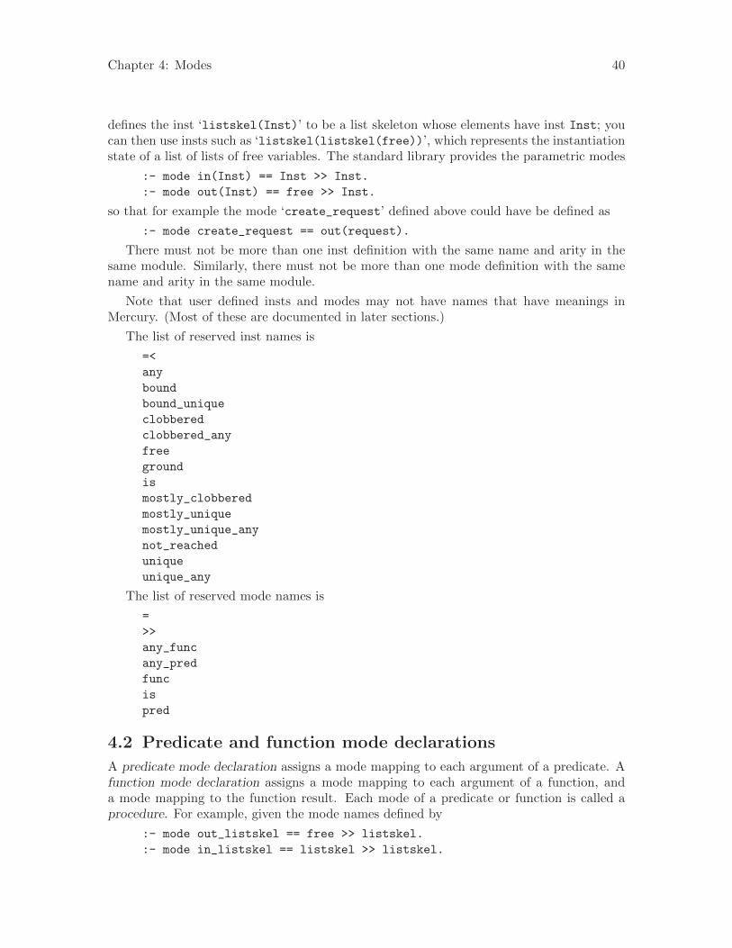
Chapter 4: Modes 40
defines the inst ‘listskel(Inst)’ to be a list skeleton whose elements have inst Inst; youcan then use insts such as ‘listskel(listskel(free))’, which represents the instantiationstate of a list of lists of free variables. The standard library provides the parametric modes
:- mode in(Inst) == Inst >> Inst.
:- mode out(Inst) == free >> Inst.
so that for example the mode ‘create_request’ defined above could have be defined as
:- mode create_request == out(request).
There must not be more than one inst definition with the same name and arity in thesame module. Similarly, there must not be more than one mode definition with the samename and arity in the same module.
Note that user defined insts and modes may not have names that have meanings inMercury. (Most of these are documented in later sections.)
The list of reserved inst names is
=<
any
bound
bound_unique
clobbered
clobbered_any
free
ground
is
mostly_clobbered
mostly_unique
mostly_unique_any
not_reached
unique
unique_any
The list of reserved mode names is
=
>>
any_func
any_pred
func
is
pred
4.2 Predicate and function mode declarations
A predicate mode declaration assigns a mode mapping to each argument of a predicate. Afunction mode declaration assigns a mode mapping to each argument of a function, anda mode mapping to the function result. Each mode of a predicate or function is called aprocedure. For example, given the mode names defined by
:- mode out_listskel == free >> listskel.
:- mode in_listskel == listskel >> listskel.

Chapter 4: Modes 41
the (type and) mode declarations of the function ‘length’ and predicate ‘append’ are asfollows:
:- func length(list(T)) = int.
:- mode length(in_listskel) = out.
:- mode length(out_listskel) = in.
:- pred append(list(T), list(T), list(T)).
:- mode append(in, in, out).
:- mode append(out, out, in).
Note that functions may have more than one mode, just like predicates; functions canbe reversible.
Alternately, the mode declarations for ‘length’ could use the standard library modes‘in/1’ and ‘out/1’:
:- func length(list(T)) = int.
:- mode length(in(listskel)) = out.
:- mode length(out(listskel)) = in.
As for type declarations, a predicate or function can be defined to have a given higher-order inst (see Section 8.3 [Higher-order insts and modes], page 62) by using ‘with_inst‘
in the mode declaration.
For example,
:- inst foldl_pred == (pred(in, in, out) is det).
:- inst foldl_func == (func(in, in) = out is det).
:- mode p(in) ‘with_inst‘ foldl_pred.
:- mode f(in) ‘with_inst‘ foldl_func.
is equivalent to
:- mode p(in, in, in, out) is det.
:- mode f(in, in, in) = out is det.
(‘is det’ is explained in Chapter 6 [Determinism], page 48.)
If a predicate or function has only one mode, the ‘pred’ and ‘mode’ declaration can becombined:
:- func length(list(T)::in) = (int::out).
:- pred append(list(T)::in, list(T)::in, list(T)::out).
:- pred p ‘with_type‘ foldl_pred(T, U) ‘with_inst‘ foldl_pred.
It is an error for a predicate or function whose ‘pred’ and ‘mode’ declarations are socombined to have any other separate ‘mode’ declarations.
If there is no mode declaration for a function, the compiler assumes a default mode forthe function in which all the arguments have mode in and the result of the function hasmode out. (However, there is no requirement that a function have such a mode; if there isany explicit mode declaration, it overrides the default.)
If a predicate or function type declaration occurs in the interface section of a module,then all mode declarations for that predicate or function must occur in the interface section
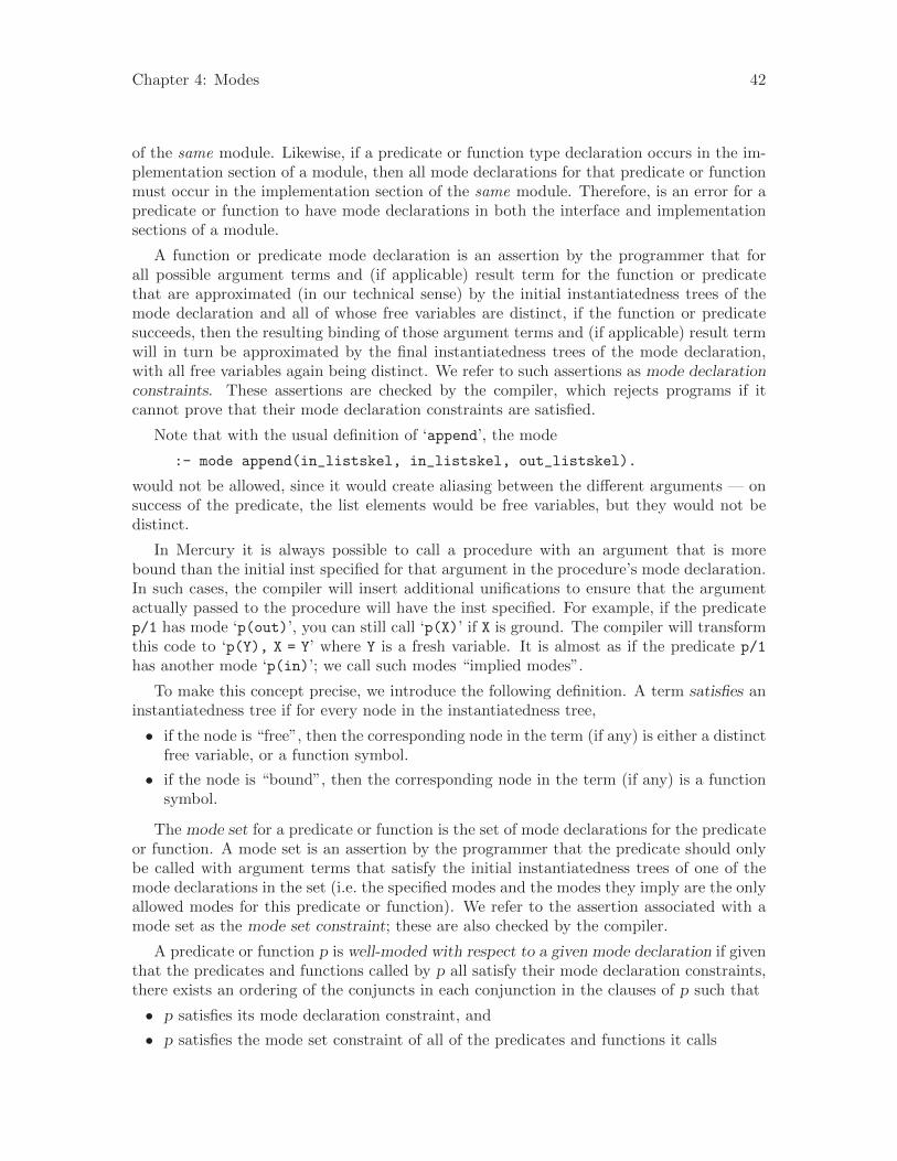
Chapter 4: Modes 42
of the same module. Likewise, if a predicate or function type declaration occurs in the im-plementation section of a module, then all mode declarations for that predicate or functionmust occur in the implementation section of the same module. Therefore, is an error for apredicate or function to have mode declarations in both the interface and implementationsections of a module.
A function or predicate mode declaration is an assertion by the programmer that forall possible argument terms and (if applicable) result term for the function or predicatethat are approximated (in our technical sense) by the initial instantiatedness trees of themode declaration and all of whose free variables are distinct, if the function or predicatesucceeds, then the resulting binding of those argument terms and (if applicable) result termwill in turn be approximated by the final instantiatedness trees of the mode declaration,with all free variables again being distinct. We refer to such assertions as mode declarationconstraints. These assertions are checked by the compiler, which rejects programs if itcannot prove that their mode declaration constraints are satisfied.
Note that with the usual definition of ‘append’, the mode
:- mode append(in_listskel, in_listskel, out_listskel).
would not be allowed, since it would create aliasing between the different arguments — onsuccess of the predicate, the list elements would be free variables, but they would not bedistinct.
In Mercury it is always possible to call a procedure with an argument that is morebound than the initial inst specified for that argument in the procedure’s mode declaration.In such cases, the compiler will insert additional unifications to ensure that the argumentactually passed to the procedure will have the inst specified. For example, if the predicatep/1 has mode ‘p(out)’, you can still call ‘p(X)’ if X is ground. The compiler will transformthis code to ‘p(Y), X = Y’ where Y is a fresh variable. It is almost as if the predicate p/1
has another mode ‘p(in)’; we call such modes “implied modes”.
To make this concept precise, we introduce the following definition. A term satisfies aninstantiatedness tree if for every node in the instantiatedness tree,
• if the node is “free”, then the corresponding node in the term (if any) is either a distinctfree variable, or a function symbol.
• if the node is “bound”, then the corresponding node in the term (if any) is a functionsymbol.
The mode set for a predicate or function is the set of mode declarations for the predicateor function. A mode set is an assertion by the programmer that the predicate should onlybe called with argument terms that satisfy the initial instantiatedness trees of one of themode declarations in the set (i.e. the specified modes and the modes they imply are the onlyallowed modes for this predicate or function). We refer to the assertion associated with amode set as the mode set constraint; these are also checked by the compiler.
A predicate or function p is well-moded with respect to a given mode declaration if giventhat the predicates and functions called by p all satisfy their mode declaration constraints,there exists an ordering of the conjuncts in each conjunction in the clauses of p such that
• p satisfies its mode declaration constraint, and
• p satisfies the mode set constraint of all of the predicates and functions it calls
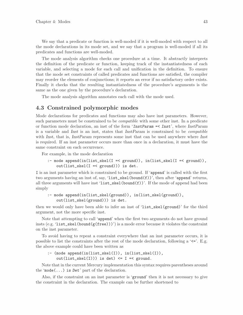
Chapter 4: Modes 43
We say that a predicate or function is well-moded if it is well-moded with respect to allthe mode declarations in its mode set, and we say that a program is well-moded if all itspredicates and functions are well-moded.
The mode analysis algorithm checks one procedure at a time. It abstractly interpretsthe definition of the predicate or function, keeping track of the instantiatedness of eachvariable, and selecting a mode for each call and unification in the definition. To ensurethat the mode set constraints of called predicates and functions are satisfied, the compilermay reorder the elements of conjunctions; it reports an error if no satisfactory order exists.Finally it checks that the resulting instantiatedness of the procedure’s arguments is thesame as the one given by the procedure’s declaration.
The mode analysis algorithm annotates each call with the mode used.
4.3 Constrained polymorphic modes
Mode declarations for predicates and functions may also have inst parameters. However,such parameters must be constrained to be compatible with some other inst. In a predicateor function mode declaration, an inst of the form ‘InstParam =< Inst ’, where InstParamis a variable and Inst is an inst, states that InstParam is constrained to be compatiblewith Inst, that is, InstParam represents some inst that can be used anywhere where Instis required. If an inst parameter occurs more than once in a declaration, it must have thesame constraint on each occurrence.
For example, in the mode declaration
:- mode append(in(list_skel(I =< ground)), in(list_skel(I =< ground)),
out(list_skel(I =< ground))) is det.
I is an inst parameter which is constrained to be ground. If ‘append’ is called with the firsttwo arguments having an inst of, say, ‘list_skel(bound(f))’, then after ‘append’ returns,all three arguments will have inst ‘list_skel(bound(f))’. If the mode of append had beensimply
:- mode append(in(list_skel(ground)), in(list_skel(ground)),
out(list_skel(ground))) is det.
then we would only have been able to infer an inst of ‘list_skel(ground)’ for the thirdargument, not the more specific inst.
Note that attempting to call ‘append’ when the first two arguments do not have groundinsts (e.g. ‘list_skel(bound(g(free)))’) is a mode error because it violates the constrainton the inst parameter.
To avoid having to repeat a constraint everywhere that an inst parameter occurs, it ispossible to list the constraints after the rest of the mode declaration, following a ‘<=’. E.g.the above example could have been written as
:- (mode append(in(list_skel(I)), in(list_skel(I)),
out(list_skel(I))) is det) <= I =< ground.
Note that in the current Mercury implementation this syntax requires parentheses aroundthe ‘mode(...) is Det ’ part of the declaration.
Also, if the constraint on an inst parameter is ‘ground’ then it is not necessary to givethe constraint in the declaration. The example can be further shortened to

Chapter 4: Modes 44
:- mode append(in(list_skel(I)), in(list_skel(I)), out(list_skel(I)))
is det.
Constrained polymorphic modes are particularly useful when passing objects with higher-order types to polymorphic predicates, since they allow the higher-order mode informationto be retained (see Chapter 8 [Higher-order], page 59).
4.4 Different clauses for different modes
Because the compiler automatically reorders conjunctions to satisfy the modes, it is oftenpossible for a single clause to satisfy different modes. However, occasionally reordering ofconjunctions is not sufficient; you may want to write different code for different modes.
For example, the usual code for list append
append([], Ys, Ys).
append([X|Xs], Ys, [X|Zs]) :-
append(Xs, Ys, Zs).
works fine in most modes, but is not very satisfactory for the ‘append(out, in, in)’ modeof append, because although every call in this mode only has at most one solution, thecompiler’s determinism inference will not be able to infer that. This means that usingthe usual code for append in this mode will be inefficient, and the overly conservativedeterminism inference may cause spurious determinism errors later.
For this mode, it is better to use a completely different algorithm:
append(Prefix, Suffix, List) :-
list.length(List, ListLength),
list.length(Suffix, SuffixLength),
PrefixLength = ListLength - SuffixLength,
list.split_list(PrefixLength, List, Prefix, Suffix).
However, that code doesn’t work in the other modes of ‘append’.
To handle such cases, you can use mode annotations on clauses, which indicate thatparticular clauses should only be used for particular modes. To specify that a clause onlyapplies to a given mode, each argument Arg of the clause head should be annotated withthe corresponding argument mode Mode, using the ‘::’ mode qualification operator, i.e.‘Arg :: Mode ’.
For example, if ‘append’ was declared as
:- pred append(list(T), list(T), list(T)).
:- mode append(in, in, out).
:- mode append(out, out, in).
:- mode append(in, out, in).
:- mode append(out, in, in).
then you could implement it as
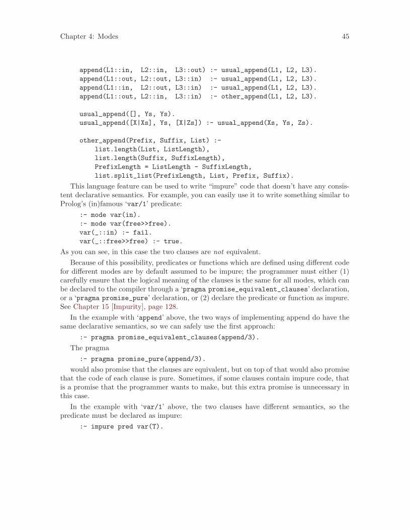
Chapter 4: Modes 45
append(L1::in, L2::in, L3::out) :- usual_append(L1, L2, L3).
append(L1::out, L2::out, L3::in) :- usual_append(L1, L2, L3).
append(L1::in, L2::out, L3::in) :- usual_append(L1, L2, L3).
append(L1::out, L2::in, L3::in) :- other_append(L1, L2, L3).
usual_append([], Ys, Ys).
usual_append([X|Xs], Ys, [X|Zs]) :- usual_append(Xs, Ys, Zs).
other_append(Prefix, Suffix, List) :-
list.length(List, ListLength),
list.length(Suffix, SuffixLength),
PrefixLength = ListLength - SuffixLength,
list.split_list(PrefixLength, List, Prefix, Suffix).
This language feature can be used to write “impure” code that doesn’t have any consis-tent declarative semantics. For example, you can easily use it to write something similar toProlog’s (in)famous ‘var/1’ predicate:
:- mode var(in).
:- mode var(free>>free).
var(_::in) :- fail.
var(_::free>>free) :- true.
As you can see, in this case the two clauses are not equivalent.
Because of this possibility, predicates or functions which are defined using different codefor different modes are by default assumed to be impure; the programmer must either (1)carefully ensure that the logical meaning of the clauses is the same for all modes, which canbe declared to the compiler through a ‘pragma promise_equivalent_clauses’ declaration,or a ‘pragma promise_pure’ declaration, or (2) declare the predicate or function as impure.See Chapter 15 [Impurity], page 128.
In the example with ‘append’ above, the two ways of implementing append do have thesame declarative semantics, so we can safely use the first approach:
:- pragma promise_equivalent_clauses(append/3).
The pragma
:- pragma promise_pure(append/3).
would also promise that the clauses are equivalent, but on top of that would also promisethat the code of each clause is pure. Sometimes, if some clauses contain impure code, thatis a promise that the programmer wants to make, but this extra promise is unnecessary inthis case.
In the example with ‘var/1’ above, the two clauses have different semantics, so thepredicate must be declared as impure:
:- impure pred var(T).
Chapter 5: Unique modes 46
5 Unique modes
Mode declarations can also specify so-called “unique modes”. Mercury’s unique modes aresimilar to “linear types” in some functional programming languages such as Clean. Theyallow you to specify when there is only one reference to a particular value, and when therewill be no more references to that value. If the compiler knows there will be no morereferences to a value, it can perform “compile-time garbage collection” by automaticallyinserting code to deallocate the storage associated with that value. Even more importantly,the compiler can also simply reuse the storage immediately, for example by destructivelyupdating one element of an array rather than making a new copy of the entire array inorder to change one element. Unique modes are also the mechanism Mercury uses toprovide declarative I/O.
We have not yet implemented unique modes fully, and the details are still in a state offlux. So the following should be considered tentative.
5.1 Destructive update
In addition to the insts mentioned above (free, ground, and bound(...)), Mercury alsoprovides “unique” insts unique and unique(...) which are like ground and bound(...)
respectively, except that they carry the additional constraint that there can only be onereference to the corresponding value. There is also an inst dead which means that thereare no references to the corresponding value, so the compiler is free to generate code thatreuses that value. There are three standard modes for manipulating unique values:
% unique output
:- mode uo == free >> unique.
% unique input
:- mode ui == unique >> unique.
% destructive input
:- mode di == unique >> dead.
Mode uo is used to create a unique value. Mode ui is used to inspect a unique valuewithout losing its uniqueness. Mode di is used to deallocate or reuse the memory occupiedby a value that will not be used.
Note that a value is not considered unique if it might be needed on backtracking. Thismeans that unique modes are generally only useful for code whose determinism is det orcc_multi (see Chapter 6 [Determinism], page 48).
Unlike bound instantiatedness trees, there is no alternative syntax for unique instanti-atedness trees.
5.2 Backtrackable destructive update
“Well it just so happens that your friend here is only mostly dead.There’s a big difference between mostly dead and all dead. . .Now, mostly dead is slightly alive.Now, all dead — well, with all dead, there’s usually only one thing that youcan do.”
Chapter 5: Unique modes 47
“What’s that?”
“Go through his clothes and look for loose change!”
— from the movie “The Princess Bride”.
To allow for backtrackable destructive updates — that is, updates whose effect is undoneon backtracking, perhaps by recording the overwritten values on a “trail” so that they canbe restored after backtracking — Mercury also provides “mostly unique” modes. The instsmostly_unique and mostly_dead are equivalent to unique and dead, except that onlyreferences which will be encountered during forward execution are counted — it is OK formostly_unique or mostly_dead values to be needed again on backtracking.
Mercury defines some standard modes for manipulating “mostly unique” values, just asit does for unique values:
% mostly unique output
:- mode muo == free >> mostly_unique.
% mostly unique input
:- mode mui == mostly_unique >> mostly_unique.
% mostly destructive input
:- mode mdi == mostly_unique >> mostly_dead.
5.3 Limitations of the current implementation
The implementation of the mode analysis algorithm is not quite complete; as a result, itis not possible to use nested unique modes, i.e. modes in which anything but the top levelof a variable is unique. If you do, you will get unique mode errors when you try to get aunique field of a unique data structure. It is also not possible to use unique-input modes;only destructive-input and unique-output modes work.
The Mercury compiler does not (yet) reuse dead values. The only destructive updatein the current implementation occurs in library modules, e.g. for I/O and arrays. Wedo however plan to implement structure reuse and compile-time garbage collection in thefuture.

Chapter 6: Determinism 48
6 Determinism
6.1 Determinism categories
For each mode of a predicate or function, we categorise that mode according to how manytimes it can succeed, and whether or not it can fail before producing its first solution.
If all possible calls to a particular mode of a predicate or function which return to thecaller (calls which terminate, do not throw an exception and do not cause a fatal runtimeerror)
• have exactly one solution, then that mode is deterministic (det);
• either have no solutions or have one solution, then that mode is semideterministic(semidet);
• have at least one solution but may have more, then that mode is multisolution (multi);
• have zero or more solutions, then that mode is nondeterministic (nondet);
• fail without producing a solution, then that mode has a determinism of failure.
If no possible calls to a particular mode of a predicate or function can return to thecaller, then that mode has a determinism of erroneous.
The determinism annotation erroneous is used on the library predicates‘require.error/1’ and ‘exception.throw/1’, but apart from that, determinismannotations erroneous and failure are generally not needed.
To summarize:
Maximum number of solutions
Can fail? 0 1 > 1
no erroneous det multi
yes failure semidet nondet
(Note: the “Can fail?” column here indicates only whether the procedure can fail beforeproducing at least one solution; attempts to find a second solution to a particular call, e.g.for a procedure with determinism multi, are always allowed to fail.)
The determinism of each mode of a predicate or function is indicated by an annotationon the mode declaration. For example:
:- pred append(list(T), list(T), list(T)).
:- mode append(in, in, out) is det.
:- mode append(out, out, in) is multi.
:- mode append(in, in, in) is semidet.
:- func length(list(T)) = int.
:- mode length(in) = out is det.
:- mode length(in(list_skel)) = out is det.
:- mode length(in) = in is semidet.
An annotation of det or multi is an assertion that for every value each of the inputs,there exists at least one value of the outputs for which the predicate is true, or (in thecase of functions) for which the function term is equal to the result term. Conversely, anannotation of det or semidet is an assertion that for every value each of the inputs, there

Chapter 6: Determinism 49
exists at most one value of the outputs for which the predicate is true, or (in the case offunctions) for which the function term is equal to the result term. These assertions are calledthe mode-determinism assertions; they can play a role in the semantics, because in certaincircumstances, they may allow an implementation to perform optimizations that would nototherwise be allowed, such as optimizing away a goal with no outputs even though it mightinfinitely loop.
If the mode of the predicate is given in the :- pred declaration rather than in a separate:- mode declaration, then the determinism annotation goes on the :- pred declaration(and similarly for functions). In particular, this is necessary if a predicate does not haveany argument variables. If the determinism declaration is given on a :- func declarationwithout the mode, the function is assumed to have the default mode (see Chapter 4 [Modes],page 38 for more information on default modes of functions).
For example:
:- pred loop(int::in) is erroneous.
loop(X) :- loop(X).
:- pred p is det.
p.
:- pred q is failure.
q :- fail.
If there is no mode declaration for a function, then the default mode for that functionis considered to have been declared as det. If you want to write a partial function, i.e. onewhose determinism is semidet, then you must explicitly declare the mode and determinism.
In Mercury, a function is supposed to be a true mathematical function of its arguments;that is, the value of the function’s result should be determined only by the values of itsarguments. Hence, for any mode of a function that specifies that all the arguments are fullyinput (i.e. for which the initial inst of all the arguments is a ground inst), the determinismof that mode can only be det, semidet, erroneous, or failure.
The determinism categories form this lattice:
erroneous
/ \
failure det
\ / \
semidet multi
\ /
nondet
The higher up this lattice a determinism category is, the more the compiler knows aboutthe number of solutions of procedures of that determinism.
6.2 Determinism checking and inference
The determinism of goals is inferred from the determinism of their component parts, ac-cording to the rules below. The inferred determinism of a procedure is just the inferreddeterminism of the procedure’s body.
Chapter 6: Determinism 50
For procedures that are local to a module, the determinism annotations may be omit-ted; in that case, their determinism will be inferred. (To be precise, the determinism ofprocedures without a determinism annotation is defined as the least fixpoint of the trans-formation which, given an initial assignment of the determinism det to all such procedures,applies those rules to infer a new determinism assignment for those procedures.)
It is an error to omit the determinism annotation for procedures that are exported fromtheir containing module.
If a determinism annotation is supplied for a procedure, the declared determinism iscompared against the inferred determinism. If the declared determinism is greater than ornot comparable to the inferred determinism (in the partial ordering above), it is an error.If the declared determinism is less than the inferred determinism, it is not an error, but theimplementation may issue a warning.
The determinism category of each goal is inferred according to the following rules. Theserules work with the two components of determinism categories: whether the goal can failwithout producing a solution, and the maximum number of solutions of the goal (0, 1, ormore). If the inference process below reports that a goal can succeed more than once, butthe goal generates no outputs that are visible from outside the goal, and the goal is notimpure (see Chapter 15 [Impurity], page 128), then the final determinism of the goal willbe based on the goal succeeding at most once, since the compiler will implicitly prune awayany duplicate solutions.
Calls The determinism category of a call is the determinism declared or inferred forthe called mode of the called procedure.
UnificationsThe determinism of a unification is either det, semidet, or failure, dependingon its mode.
A unification that assigns the value of one variable to another is deterministic.A unification that constructs a structure and assigns it to a variable is also de-terministic. A unification that tests whether a variable has a given top functionsymbol is semideterministic, unless the compiler knows the top function symbolof that variable, in which case its determinism is either det or failure dependingon whether the two function symbols are the same or not. A unification thattests two variables for equality is semideterministic, unless the compiler knowsthat the two variables are aliases for one another, in which case the unificationis deterministic, or unless the compiler knows that the two variables have dif-ferent function symbols in the same position, in which case the unification hasa determinism of failure.
The compiler knows the top function symbol of a variable if the previous partof the procedure definition contains a unification of the variable with a functionsymbol, or if the variable’s type has only one function symbol.
ConjunctionsThe determinism of the empty conjunction (the goal ‘true’) is det. The con-junction ‘(A, B)’ can fail if either A can fail, or if A can succeed at least once,and B can fail. The conjunction can succeed at most zero times if either A or Bcan succeed at most zero times. The conjunction can succeed more than once

Chapter 6: Determinism 51
if either A or B can succeed more than once and both A and B can succeed atleast once. (If e.g. A can succeed at most zero times, then even if B can suc-ceed many times the maximum number of solutions of the conjunction is stillzero.) Otherwise, i.e. if both A and B succeed at most once, the conjunctioncan succeed at most once.
Switches A disjunction is a switch if each disjunct has near its start a unification thattests the same bound variable against a different function symbol. For example,consider the common pattern
(
L = [], empty(Out)
;
L = [H|T], nonempty(H, T, Out)
)
If L is input to the disjunction, then the disjunction is a switch on L.
If two variables are unified with each other, then whatever function symbol onevariable is unified with, the other variable is considered to be unified with thesame function symbol. In the following example, since K is unified with L, thesecond disjunct unifies L as well as K with cons, and thus the disjunction isrecognized as a switch.
(
L = [], empty(Out)
;
K = L, K = [H|T], nonempty(H, T, Out)
)
A switch can fail if the various arms of the switch do not cover all the functionsymbols in the type of the switched-on variable, or if the code in some armsof the switch can fail, bearing in mind that in each arm of the switch, theunification that tests the switched-on variable against the function symbol ofthat arm is considered to be deterministic. A switch can succeed several timesif some arms of the switch can succeed several times, possibly because there aremultiple disjuncts that test the switched-on variable against the same functionsymbol. A switch can succeed at most zero times only if all the reachable armsof the switch can succeed at most zero times. (A switch arm is not reachable ifit unifies the switched-on variable with a function symbol that is ruled out bythat variable’ initial instantation state.)
Only unifications may occur before the test of the switched-on variable in eachdisjunct. Tests of the switched-on variable may occur within existential quan-tification goals.
The following example is a switch.
(
Out = 1, L = []
;
some [H, T] (
L = [H|T],
nonempty(H, T, Out)

Chapter 6: Determinism 52
)
)
The following example is not a switch because the call in the first disjunctoccurs before the test of the switched-on variable.
(
empty(Out), L = []
;
L = [H|T], nonempty(H, T, Out)
)
The unification of the switched-on variable with a function symbol may occurinside a nested disjunction in a given disjunct, provided that unification ispreceded only by other unifications, both inside the nested disjunction andbefore the nested disjunction. The following example is a switch on X, providedX is bound beforehand.
(
X = f
p(Out)
;
Y = X,
(
Y = g,
Intermediate = 42
;
Z = Y,
Z = h(Arg),
q(Arg, Intermediate)
),
r(Intermediate, Out)
)
DisjunctionsThe determinism of the empty disjunction (the goal ‘fail’) is failure. Adisjunction ‘(A ; B)’ that is not a switch can fail if both A and B can fail. Itcan succeed at most zero times if both A and B can succeed at most zero times.It can succeed at most once if one of A and B can succeed at most once andthe other can succeed at most zero times. Otherwise, i.e. if either A or B cansucceed more than once, or if both A and B can succeed at least once, it cansucceed more than once.
If-then-elseIf the condition of an if-then-else cannot fail, the if-then-else is equivalent tothe conjunction of the condition and the “then” part, and its determinism iscomputed accordingly. Otherwise, an if-then-else can fail if either the “then”part or the “else” part can fail. It can succeed at most zero times if the “else”part can succeed at most zero times and if at least one of the condition and the“then” part can succeed at most zero times. It can succeed more than once if

Chapter 6: Determinism 53
any one of the condition, the “then” part and the “else” part can succeed morethan once.
Negations
If the determinism of the negated goal is erroneous, then the determinism ofthe negation is erroneous. If the determinism of the negated goal is failure,the determinism of the negation is det. If the determinism of the negated goalis det or multi, the determinism of the negation is failure. Otherwise, thedeterminism of the negation is semidet.
6.3 Replacing compile-time checking with run-time checking
Note that “perfect” determinism inference is an undecidable problem, because it requiressolving the halting problem. (For instance, in the following example
:- pred p(T, T).
:- mode p(in, out) is det.
p(A, B) :-
(
something_complicated(A, B)
;
B = A
).
‘p/2’ can have more than one solution only if ‘something_complicated/2’ can succeed.)Sometimes, the rules specified by the Mercury language for determinism inference will infera determinism that is not as precise as you would like. However, it is generally easy toovercome such problems. The way to do this is to replace the compiler’s static checkingwith some manual run-time checking. For example, if you know that a particular goalshould never fail, but the compiler infers that goal to be semidet, you can check at runtimethat the goal does succeed, and if it fails, call the library predicate ‘error/1’.
:- pred q(T, T).
:- mode q(in, out) is det.
q(A, B) :-
( goal_that_should_never_fail(A, B0) ->
B = B0
;
error("goal_that_should_never_fail failed!")
).
The predicate error/1 has determinism erroneous, which means the compiler knows that itwill never succeed or fail, so the inferred determinism for the body of q/2 is det. (Checkingassumptions like this is good coding style anyway. The small amount of up-front workthat Mercury requires is paid back in reduced debugging time.) Mercury’s mode analysisknows that computations with determinism erroneous can never succeed, which is why itdoes not require the “else” part to generate a value for B. The introduction of the newvariable B0 is necessary because the condition of an if-then-else is a negated context, andcan export the values it generates only to the “then” part of the if-then-else, not directly to

Chapter 6: Determinism 54
the surrounding computation. (If the surrounding computations had direct access to valuesgenerated in conditions, they might access them even if the condition failed.)
6.4 Interfacing nondeterministic code with the real world
Normally, attempting to call a nondet or multi mode of a predicate from a predicatedeclared as semidet or det will cause a determinism error. So how can we call nondeter-ministic code from deterministic code? There are several alternative possibilities.
If you just want to see if a nondeterministic goal is satisfiable or not, without needing toknow what variable bindings it produces, then there is no problem - determinism analysisconsiders nondet and multi goals with no non-local output variables to be semidet anddet respectively.
If you want to use the values of output variables, then you need to ask yourself whichone of possibly many solutions to a goal do you want? If you want all of them, you need touse the predicate ‘solutions/2’ in the standard library module ‘solutions’, which collectsall of the solutions to a goal into a list — see Chapter 8 [Higher-order], page 59.
If you just want one solution and don’t care which, the calling predicate should bedeclared nondet or multi. The nondeterminism should then be propagated up the call treeto the point at which it can be pruned. In Mercury, pruning can be achieved in severalways.
The first way is the one mentioned above: if a goal has no non-local output variablesthen the implementation will only attempt to satisfy the goal once. Any potential duplicatesolutions will be implicitly pruned away.
The second way is to rely on the fact that the implementation will only seek a singlesolution to ‘main/2’, so alternative solutions to ‘main/2’ (and hence also to nondet or multipredicates called directly or indirectly from ‘main/2’) are implicitly pruned away. This isone way to achieve “don’t care” style nondeterminism in Mercury.
The other situation in which you may want pruning and committed choice style nonde-terminism is when you know that all the solutions returned will be equivalent. For example,you might want to find the maximum element in a set by iterating over the elements inthe set. Iterating over the elements in a set in an unspecified order is a nondeterministicoperation, but no matter which order you remove them, the maximum value in the setshould be the same.
If you know that there will only ever be at most one distinct solution under the equal-ity theory of the output variables, then you can use a ‘promise_equivalent_solutions’determinism cast.
Note that specifying a user-defined equivalence relation as the equality predicate foruser-defined types (see Chapter 7 [User-defined equality and comparison], page 56) meansthat ‘promise_equivalent_solutions’ can be used to express more general forms of equiv-alence. For example, if you define a set type which represents sets as unsorted lists, youwould want to define a user-defined equivalence relation for that type, which could sortthe lists before comparing them. The ‘promise_equivalent_solutions’ determinism castcould then be used for sets even though the lists used to represent the sets might not be inthe same order in every solution.

Chapter 6: Determinism 55
6.5 Committed choice nondeterminism
In addition to the determinism annotations described earlier, there are “committed choice”versions of multi and nondet, called cc_multi and cc_nondet. These can be used insteadof multi or nondet if all calls to that mode of the predicate (or function) occur in a contextin which only one solution is needed.
Such single-solution contexts are determined as follows.
• The body of any procedure declared cc_multi or cc_nondet is in a single-solutioncontext. For example, the program entry point ‘main/2’ may be declared cc_multi,and in that case the clauses for main are in a single-solution context.
• Any goal with no output variables is in a single-solution context.
• If a conjunction is in a single-solution context, then the right-most conjunct is in asingle-solution context, and if the right-most conjunct cannot fail, then the rest of theconjunction is also in a single-solution context. (“Right-most” here refers to the orderafter mode reordering.)
• If an if-then-else is in a single-solution context, then the “then” part and the “else” partare in single-solution contexts, and if the “then” part cannot fail, then the conditionof the if-then-else is also in a single-solution context.
• For other compound goals, i.e. disjunctions, negations, and (explicitly) existentiallyquantified goals, if the compound goal is in a single-solution context, then the imme-diate sub-goals of that compound goal are also in single-solution contexts.
The compiler will check that all calls to a committed-choice mode of a predicate (orfunction) do indeed occur in a single-solution context.
You can declare two different modes of a predicate (or function) which differ only in“cc-ness” (i.e. one being multi and the other cc_multi, or one being nondet and theother cc_nondet). In that case, the compiler will select the appropriate one for each calldepending on whether the call comes from a single-solution context or not. Calls fromsingle-solution contexts will call the committed choice version, while calls which are notfrom single-solution contexts will call the backtracking version.
There are several reasons to use committed choice determinism annotations. One reasonis for efficiency: committed choice annotations allow the compiler to generate much moreefficient code. Another reason is for doing I/O, which is allowed only in det or cc_multipredicates, not in multi predicates. Another is for dealing with types that use non-canonicalrepresentations (see Chapter 7 [User-defined equality and comparison], page 56). And thereare a variety of other applications.
Chapter 7: User-defined equality and comparison 56
7 User-defined equality and comparison
When defining abstract data types, often it is convenient to use a non-canonical represen-tation — that is, one for which a single abstract value may have more than one differentpossible concrete representation. For example, you may wish to implement an abstract type‘set’ by representing a set as an (unsorted) list.
:- module set_as_unsorted_list.
:- interface.
:- type set(T).
:- implementation.
:- import_module list.
:- type set(T)
---> set(list(T)).
In this example, the concrete representations ‘set([1,2])’ and ‘set([2,1])’ would bothrepresent the same abstract value, namely the set containing the elements 1 and 2.
For types such as this, which do not have a canonical representation, the standarddefinition of equality is not the desired one; we want equality on sets to mean equality ofthe abstract values, not equality of their representations. To support such types, Mercuryallows programmers to specify a user-defined equality predicate for user-defined types:
:- type set(T)
---> set(list(T))
where equality is set_equals.
Here ‘set_equals’ is the name of a user-defined predicate that is used for equality on thetype ‘set(T)’. It could for example be defined in terms of a ‘subset’ predicate.
:- pred set_equals(set(T)::in, set(T)::in) is semidet.
set_equals(S1, S2) :-
subset(S1, S2),
subset(S2, S1).
A comparison predicate can also be supplied.
:- type set(T)
---> set(list(T))
where equality is set_equals, comparison is set_compare.
:- pred set_compare(builtin.comparison_result::uo,
set(T)::in, set(T)::in) is det.
set_compare(Result, Set1, Set2) :-
promise_equivalent_solutions [Result] (
set_compare_2(Set1, Set2, Result)
).
:- pred set_compare_2(set(T)::in, set(T)::in,
builtin.comparison_result::uo) is cc_multi.

Chapter 7: User-defined equality and comparison 57
set_compare_2(set(List1), set(List2), Result) :-
builtin.compare(Result, list.sort(List1), list.sort(List2)).
If a comparison predicate is supplied and the unification predicate is omitted, a unifica-tion predicate is generated by the compiler in terms of the comparison predicate. For the‘set’ example, the generated predicate would be:
set_equals(S1, S2) :-
set_compare((=), S1, S2).
If a unification predicate is supplied without a comparison predicate, thecompiler will generate a comparison predicate which throws an exception of type‘exception.software_error’ when called.
A type declaration for a type ‘foo(T1, ..., TN)’ may contain a ‘where equality is
equalitypred ’ specification only if it declares a discriminated union type or a foreign type(see Section 14.4 [Using foreign types from Mercury], page 108) and the following conditionsare satisfied:
• equalitypred must be the name of a predicate with signature
:- pred equalitypred(foo(T1, ..., TN)::in,
foo(T1, ..., TN)::in) is semidet.
It is legal for the type, mode and determinism to be more permissive: the type orthe mode’s initial insts may be more general (e.g. the type of the equality predicatecould be just the polymorphic type ‘pred(T, T)’) and the mode’s final insts or thedeterminism may be more specific (e.g. the determinism of the equality predicate couldbe any of det, failure or erroneous).
• If the type is a discriminated union then its definition cannot be a single zero-arityconstructor.
• The equality predicate must be “pure” (see Chapter 15 [Impurity], page 128).
• The equality predicate must be defined in the same module as the type.
• If the type is exported the equality predicate must also be exported.
• equalitypred should be an equivalence relation; that is, it must be symmetric, reflexive,and transitive. However, the compiler is not required to check this1.
Types with user-defined equality can only be used in limited ways. Because there aremultiple representations for the same abstract value, any attempt to examine the repre-sentation of such a value is a conceptually non-deterministic operation. In Mercury this ismodelled using committed choice nondeterminism.
The semantics of specifying ‘where equality is equalitypred ’ on the type declarationfor a type T are as follows:
• If the program contains any deconstruction unification or switch on a variable of type Tthat could fail, other than unifications with mode ‘(in, in)’, then it is a compile-timeerror.
1 If equalitypred is not an equivalence relation, then the program is inconsistent: its declarative semanticscontains a contradiction, because the additional axioms for the user-defined equality contradict thestandard equality axioms. That implies that the implementation may compute any answer at all (seeChapter 13 [Semantics], page 95), i.e. the behaviour of the program is undefined.
Chapter 7: User-defined equality and comparison 58
• If the program contains any deconstruction unification or switch on a variable of typeT that cannot fail, then that operation has determinism cc_multi.
• Any attempts to examine the representation of a variable of type T using facilities ofthe standard library (e.g. ‘argument’/3 and ‘functor/3’ in ‘deconstruct’) that do nothave determinism cc_multi or cc_nondet will result in a run-time error.
• In addition to the usual equality axioms, the declarative semantics of the program willcontain the axiom ‘X = Y <=> equalitypred(X, Y)’ for all X and Y of type ‘T’.
• Any ‘(in, in)’ unifications for type T are computed using the specified predicateequalitypred.
A type declaration for a type ‘foo(T1, ..., TN)’ may contain a ‘where comparison is
comparepred ’ specification only if it declares a discriminated union type or a foreign type(see Section 14.4 [Using foreign types from Mercury], page 108) and the following conditionsare satisfied:
• comparepred must be the name of a predicate with signature
:- pred comparepred(builtin.comparison_result::uo,
foo(T1, ..., TN)::in, foo(T1, ..., TN)::in) is det.
As with equality predicates, it is legal for the type, mode and determinism to be morepermissive.
• If the type is a discriminated union then its definition cannot be a single zero-arityconstructor.
• The comparison predicate must also be “pure” (see Chapter 15 [Impurity], page 128).
• The comparison predicate must be defined in the same module as the type.
• If the type is exported the comparison predicate must also be exported.
• The relation
compare_eq(X, Y) :- comparepred((=), X, Y).
must be an equivalence relation; that is, it must be symmetric, reflexive, and transitive.The compiler is not required to check this.
• The relations
compare_leq(X, Y) :- comparepred(R, X, Y), (R = (=) ; R = (<)).
compare_geq(X, Y) :- comparepred(R, X, Y), (R = (=) ; R = (>)).
must be total order relations: that is they must be antisymmetric, reflexive and tran-sitive. The compiler is not required to check this.
For each type for which the declaration has a ‘where comparison is comparepred ’ spec-ification, any calls to the standard library predicate ‘builtin.compare/3’ with argumentsof that type are evaluated as if they were calls to comparepred.
A type declaration may contain a ‘where equality is equalitypred, comparison is
comparepred ’ specification only if in addition to the conditions above, ‘all [X, Y] (com-
parepred((=), X, Y) <=> equalitypred(X, Y))’. The compiler is not required to checkthis.
Chapter 8: Higher-order programming 59
8 Higher-order programming
Mercury supports higher-order functions and predicates with currying, closures, and lambdaexpressions. (To be pedantic, it would be more accurate to say that Mercury supportshigher-order procedures: in Mercury, when you construct a higher-order term, you only getone mode of a predicate or function; if you want multiple modes, you must pass multiplehigher-order procedures.)
8.1 Creating higher-order terms
To create a higher-order predicate or function term, you can use a lambda expression, or,if the predicate or function has only one mode and it is not a zero-arity function, you canjust use its name. For example, if you have declared a predicate
:- pred sum(list(int), int).
:- mode sum(in, out) is det.
the following unifications have the same effect:
X = (pred(List::in, Length::out) is det :- sum(List, Length))
Y = sum
In the above example, the type of X, and Y is ‘pred(list(int), int)’, which means apredicate of two arguments of types list(int) and int respectively.
Similarly, given
:- func scalar_product(int, list(int)) = list(int).
:- mode scalar_product(in, in) = out is det.
the following three unifications have the same effect:
X = (func(Num, List) = NewList :- NewList = scalar_product(Num, List))
Y = (func(Num::in, List::in) = (NewList::out) is det
:- NewList = scalar_product(Num, List))
Z = scalar_product
In the above example, the type of X, Y, and Z is ‘func(int, list(int)) = list(int)’,which means a function of two arguments, whose types are int and list(int), with areturn type of int. As with ‘:- func’ declarations, if the modes and determinism of thefunction are omitted in a higher-order function term, then the modes default to in for thearguments, out for the function result, and the determinism defaults to det.
The Melbourne Mercury implementation currently requires that you use an explicitlambda expression to specify which mode you want, if the predicate or function has morethan one mode (but see below for an exception to this rule).
You can also create higher-order function terms of non-zero arity and higher-order pred-icate terms by “currying”, i.e. specifying the first few arguments to a predicate or function,but leaving the remaining arguments unspecified. For example, the unification
Sum123 = sum([1,2,3])
binds Sum123 to a higher-order predicate term of type ‘pred(int)’. Similarly, the unification
Double = scalar_product(2)
binds Double to a higher-order function term of type ‘func(list(int)) = list(int)’.
Chapter 8: Higher-order programming 60
As a special case, currying of a multi-moded predicate or function is allowed providedthat the mode of the predicate or function can be determined from the insts of the higher-order curried arguments. For example, ‘P = list.foldl(io.write)’ is allowed because theinst of ‘io.write’ matches exactly one mode of ‘list.foldl’.
For higher-order predicate expressions that thread an accumulator pair, we have syntaxthat allows you to use DCG notation in the goal of the expression. For example,
Pred = (pred(Strings::in, Num::out, di, uo) is det -->
io.write_string("The strings are: "),
{ list.length(Strings, Num) },
io.write_strings(Strings),
io.nl
)
is equivalent to
Pred = (pred(Strings::in, Num::out, IO0::di, IO::uo) is det :-
io.write_string("The strings are: ", IO0, IO1),
list.length(Strings, Num),
io.write_strings(Strings, IO1, IO2),
io.nl(IO2, IO)
)
Higher-order function terms of zero arity can only be created using an explicit lambdaexpression; you have to use e.g. ‘(func) = foo’ rather than plain ‘foo’, because the latterdenotes the result of evaluating the function, rather than the function itself.
Note that when constructing a higher-order term, you cannot just use the name of abuiltin language construct such as ‘=’, ‘\=’, ‘call’, or ‘apply’, and nor can such constructsbe curried. Instead, you must either use an explicit lambda expression, or you must writea forwarding predicate or function. For example, instead of
list.filter(\=(2), [1, 2, 3], List)
you must write either
list.filter((pred(X::in) is semidet :- X \= 2), [1, 2, 3], List)
or
list.filter(not_equal(2), [1, 2, 3], List)
where you have defined ‘not_equal’ using
:- pred not_equal(T::in, T::in) is semidet.
not_equal(X, Y) :- X \= Y.
Another case when this arises is when want to curry a higher-order term. Suppose,for example, that you have a higher-order predicate term ‘OldPred’ of type ‘pred(int,char, float)’, and you want to construct a new higher-order predicate term ‘NewPred’ oftype ‘pred(char, float)’ from ‘OldPred’ by supplying a value for just the first argument.The solution is the same: use an explicit lambda expression or a forwarding predicate. Ineither case, the body of the lambda expression or the forwarding predicate must contain ahigher-order call with all the arguments supplied.

Chapter 8: Higher-order programming 61
8.2 Calling higher-order terms
Once you have created a higher-order predicate term (sometimes known as a closure), thenext thing you want to do is to call it. For predicates, you use the builtin goal call/N:
call(Closure)
call(Closure1, Arg1)
call(Closure2, Arg1, Arg2)
. . . A higher-order predicate call. ‘call(Closure)’ just calls the specified higher-order predicate term. The other forms append the specified arguments ontothe argument list of the closure before calling it.
For example, the goal
call(Sum123, Result)
would bind Result to the sum of ‘[1, 2, 3]’, i.e. to 6.
For functions, you use the builtin expression apply/N:
apply(Closure)
apply(Closure1, Arg1)
apply(Closure2, Arg1, Arg2)
. . . A higher-order function application. Such a term denotes the result of invokingthe specified higher-order function term with the specified arguments.
For example, given the definition of ‘Double’ above, the goal
List = apply(Double, [1, 2, 3])
would be equivalent to
List = scalar_product(2, [1, 2, 3])
and so for a suitable implementation of the function ‘scalar_product/2’ this would bindList to ‘[2, 4, 6]’.
One extremely useful higher-order predicate in the Mercury standard library is‘solutions/2’, which has the following declaration:
:- pred solutions(pred(T), list(T)).
:- mode solutions(pred(out) is nondet, out) is det.
The term which you pass to ‘solutions/2’ is a higher-order predicate term. You can passthe name of a one-argument predicate, or you can pass a several-argument predicate with allbut one of the arguments supplied (a closure). The declarative semantics of ‘solutions/2’can be defined as follows:
solutions(Pred, List) is true iff
all [X] (call(Pred, X) <=> list.member(X, List))
and List is sorted.
where ‘call(Pred, X)’ invokes the higher-order predicate term Pred with argument X,and where ‘list.member/2’ is the standard library predicate for list membership. In otherwords, ‘solutions(Pred, List)’ finds all the values of X for which ‘call(Pred, X)’ is true,collects these solutions in a list, sorts the list, and returns that list as its result. Here is anexample: the standard library defines a predicate ‘list.perm(List0, List)’
Chapter 8: Higher-order programming 62
:- pred list.perm(list(T), list(T)).
:- mode list.perm(in, out) is nondet.
which succeeds iff List is a permutation of List0. Hence the following call to solutions
solutions(list.perm([3,1,2]), L)
should return all the possible permutations of the list ‘[3,1,2]’ in sorted order:
L = [[1,2,3],[1,3,2],[2,1,3],[2,3,1],[3,1,2],[3,2,1]].
See also ‘unsorted_solutions/2’ and ‘solutions_set/2’, which are defined in thestandard library module ‘solutions’ and documented in the Mercury Library ReferenceManual.
8.3 Higher-order insts and modes
In Mercury, the mode and determinism of a higher-order predicate or function term aregenerally part of that term’s inst, not its type. This allows a single higher-order predicateto work on argument predicates of different modes and determinism, which is particularlyuseful for library predicates such as ‘list.map’ and ‘list.foldl’.
8.3.1 Builtin higher-order insts and modes
The language contains builtin ‘inst’ values
(pred) is Determinism
pred(Mode) is Determinism
pred(Mode1, Mode2) is Determinism
...
(func) = Mode is Determinism
func(Mode1) = Mode is Determinism
func(Mode1, Mode2) = Mode is Determinism
...
These insts represent the instantiation state of variables bound to higher-order predicateand function terms with the appropriate mode and determinism. For example, ‘pred(out)is det’ represents the instantiation state of being bound to a higher-order predicate termwhich is det and accepts one output argument; the term ‘sum([1,2,3])’ from the exampleabove is one such higher-order predicate term which matches this instantiation state.
As a convenience, the language also contains builtin ‘mode’ values of the same name (andthey are what we have been using in the examples up to now). These modes map from thecorresponding ‘inst’ to itself. It is as if they were defined by
:- mode (pred is Determinism) == in(pred is Determinism).
:- mode (pred(Inst) is Determinism) ==
in(pred(Inst) is Determinism).
...
using the parametric inst ‘in/1’ mentioned in Chapter 4 [Modes], page 38 which maps aninst to itself.
If you want to define a predicate which returns a higher-order predicate term, you woulduse a mode such as ‘free >> pred(...) is ...’, or ‘out(pred(...) is ... )’. For exam-ple:

Chapter 8: Higher-order programming 63
:- pred foo(pred(int)).
:- mode foo(free >> pred(out) is det) is det.
foo(sum([1,2,3])).
Note that in Mercury it is an error to attempt to unify two higher-order terms. This isbecause equivalence of higher-order terms is undecidable in the general case.
For example, given the definition of ‘foo’ above, the goal
foo((pred(X::out) is det :- X = 6))
is illegal. If you really want to compare higher-order predicates for equivalence, you mustprogram it yourself; for example, the above goal could legally be written as
P = (pred(X::out) is det :- X = 6),
foo(Q),
all [X] (call(P, X) <=> call(Q, X)).
Note that the compiler will only catch direct attempts at higher-order unifications; in-direct attempts (via polymorphic predicates, for example ‘(list.append([], [P], [Q])’may result in an error at run-time rather than at compile-time.
Mercury also provides builtin ‘inst’ values for use with solver types:
any_pred is Determinism
any_pred(Mode) is Determinism
any_pred(Mode1, Mode2) is Determinism
...
any_func = Mode is Determinism
any_func(Mode1) = Mode is Determinism
any_func(Mode1, Mode2) = Mode is Determinism
...
See Chapter 16 [Solver types], page 134 for more details.
8.3.2 Default insts for functions
In order to call a higher-order term, the compiler must know its higher-order inst. Thiscan cause problems when higher-order terms are placed into a polymorphic collection typeand then extracted, since the declared mode for the extraction will typically be out andthe higher-order inst information will be lost. To partially alleviate this problem, and tomake higher-order functional programming easier, if the term to be called has a functiontype, but no higher-order inst information is explicitly provided, we assume that it has thedefault higher-order function inst ‘func(in, ..., in) = out is det’.
As a consequence of this, a higher-order function term can only be passed where a termwith no higher-order inst information is expected if it can be passed where a term with thedefault higher-order function inst is expected. Higher-order predicate terms can always bepassed to such a place, but note that there is little value in doing so because there is nodefault higher-order inst for predicates therefore it will not be possible to call those terms.
8.3.3 Combined higher-order types and insts
A higher-order type may optionally specify an inst in the following manner:

Chapter 8: Higher-order programming 64
(pred) is Determinism
pred(Type::Mode) is Determinism
pred(Type1::Mode1, Type2::Mode2) is Determinism
...
(func) = (Type::Mode) is Determinism
func(Type1::Mode1) = (Type::Mode) is Determinism
func(Type1::Mode1, Type2::Mode2) = (Type::Mode) is Determinism
...
When used as argument types of functors in type declarations, types of this form havetwo effects. First, for any unification that constructs a term using such an argument, thereis an additional mode constraint that the argument must be approximated by the inst. Inother words, to be mode correct a program must not construct any term where a functorhas an argument that does not have the declared inst, if present.
The second effect is that when a unification deconstructs a ground term to extract anargument with such a declared inst, the extracted argument may then be used as if it hadthat inst.
For example, given this type declaration:
:- type job
---> job(pred(int::out, io::di, io::uo) is det).
the following goal is correct:
:- pred run(job::in, io::di, io::uo) is det.
run(Job, !IO) :-
Job = job(Pred),
Pred(Result, !IO), % Pred has the necessary inst
write_line(Result, !IO).
However, the following would be a mode error:
:- pred bad(job::out) is det.
bad(job(p)). % Error: p does not have required mode
:- pred p(int::in, io::di, io::out) is det.
...
As a new feature, combined higher-order types and insts are only permitted as directarguments of functors in discriminated unions. So the following examples currently resultin errors.
% Error: use on the RHS of equivalence types.
:- type p == (pred(io::di, io::uo) is det).
:- type f == (func(int::in) = (int::out) is semidet).
% Error: use inside a type constructor.
:- type jobs
---> jobs(list(pred(int::out, io::di, io::uo) is det)).
% Error: use in a pred/func declaration.
:- pred p((pred(io::di, io::uo) is det)::in, io::di, io::uo) is det.
:- func f(func(int::in) = (int::out) is semidet, int) = int.

Chapter 8: Higher-order programming 65
Future versions of the language may allow these forms.
Chapter 9: Modules 66
9 Modules
9.1 The module system
The Mercury module system is relatively simple and straightforward.
Each module must start with a ‘:- module ModuleName ’ declaration, specifying the nameof the module.
An ‘:- interface.’ declaration indicates the start of the module’s interface section: thissection specifies the entities that are exported by this module. Mercury provides supportfor abstract data types, by allowing the definition of a type to be kept hidden, with theinterface only exporting the type name. The interface section may contain definitions oftypes, type classes, data constructors, instantiation states, and modes, and declarations forabstract data types, abstract type class instances, functions, predicates, and (sub-)modules.The interface section may not contain definitions for functions or predicates (i.e. clauses),or definitions of (sub-)modules.
An ‘:- implementation.’ declaration indicates the start of the module’s implementationsection. Any entities declared in this section are local to the module (and its submodules,if any) and cannot be used by other modules. The implementation section must containdefinitions for all abstract data types, abstract instance declarations, functions, predicates,and submodules exported by the module, as well as for all local types, type class instances,functions, predicates, and submodules. The implementation section can be omitted if it isempty.
The module may optionally end with a ‘:- end_module ModuleName ’ declaration; thename specified in the ‘end_module’ must be the same as that in the corresponding ‘module’declaration.
If a module wishes to make use of entities exported by other modules, then it mustexplicitly import those modules using one or more ‘:- import_module Modules ’ or‘:- use_module Modules ’ declarations, in order to make those declarations visible. Inboth cases, Modules is a comma-separated list of fully qualified module names. Thesedeclarations may occur either in the interface or the implementation section. If theimported entities are used in the interface section, then the corresponding import_module
or use_module declaration must also be in the interface section. If the imported entities areonly used in the implementation section, the import_module or use_module declarationshould be in the implementation section.
The names of predicates, functions, constructors, constructor fields, types, modes, insts,type classes, and (sub-)modules can be explicitly module qualified using the ‘.’ operator,e.g. ‘module.name’ or ‘module.submodule.name’. This is useful both for readability andfor resolving name conflicts. Uses of entities imported using use_module declarations mustbe explicitly fully module qualified.
Currently we also support ‘__’ as an alternative module qualifier, so you can writemodule__name instead of module.name.
Certain optimizations require information or source code for predicates defined in othermodules to be as effective as possible. At the moment, inlining and higher-order special-ization are the only optimizations that the Mercury compiler can perform across moduleboundaries.
Chapter 9: Modules 67
Exactly one module of the program must export a predicate ‘main/2’, which must bedeclared as either
:- pred main(io.state::di, io.state::uo) is det.
or
:- pred main(io.state::di, io.state::uo) is cc_multi.
(or any declaration equivalent to one of the two above).
Mercury has a standard library which includes over 100 modules, including modules forlists, stacks, queues, priority queues, sets, bags (multi-sets), maps (dictionaries), randomnumber generation, input/output, and filename and directory handling. See the MercuryLibrary Reference Manual for a list of the available modules, and for the documentation ofeach module.
9.2 An example module.
For illustrative purposes, here is the definition of a simple module for managing queues:
:- module queue.
:- interface.
% Declare an abstract data type.
:- type queue(T).
% Declare some predicates which operate on the abstract data type.
:- pred empty_queue(queue(T)).
:- mode empty_queue(out) is det.
:- mode empty_queue(in) is semidet.
:- pred put(queue(T), T, queue(T)).
:- mode put(in, in, out) is det.
:- pred get(queue(T), T, queue(T)).
:- mode get(in, out, out) is semidet.
:- implementation.
% Queues are implemented as lists. We need the ‘list’ module
% for the declaration of the type list(T), with its constructors
% ’[]’/0 % and ’.’/2, and for the declaration of the predicate
% list.append/3.
:- import_module list.
% Define the queue ADT.
:- type queue(T) == list(T).
Chapter 9: Modules 68
% Define the exported predicates.
empty_queue([]).
put(Queue0, Elem, Queue) :-
list.append(Queue0, [Elem], Queue).
get([Elem | Queue], Elem, Queue).
:- end_module queue.
9.3 Submodules
As mentioned above, modules may contain submodules. There are two kinds of submodules,called nested submodules and separate submodules; the difference is that nested submodulesare defined in the same source file as the containing module, whereas separate submodulesare defined in separate source files. Implementations should support separate compilationof separate submodules.
A module may not contain more than one submodule with the same name.
9.3.1 Nested submodules
Nested submodules within a module are delimited by matching ‘:- module’ and ‘:-end_module’ declarations. (Note that ‘:- end_module’ for nested submodules aremandatory, not optional, even if the nested submodule is the last thing in the source file.The module name in a ‘:- module’ or ‘:- end_module’ declaration for a nested submoduleneed not be fully qualified.) The sequence of items thus delimited is known as a submoduleitem sequence.
The interface and implementation parts of a nested submodule may be specified intwo different submodule declarations. If a submodule item sequence includes an interfacesection, then it is a declaration of that submodule; if it includes an implementation section,then it is a definition of that submodule; and if includes both, then it is both declarationand definition.
It is an error to declare a submodule twice, or to define it twice. It is an error to define asubmodule without declaring it. As mentioned earlier, it is an error to define a submodulein the interface section of its parent module.
If a submodule is declared but not explicitly defined, then there is an implicit definitionwith an empty implementation section for that submodule. This empty implementationsection will result in an error if the interface section of a submodule contains any of thefollowing:
• a declaration for a function or a predicate;
• an abstract declaration for a type, inst, mode or typeclass, i.e. a declaration that doesnot itself serve as a definition of that type, inst, mode or typeclass;
• an abstract declaration of a typeclass instance; or
• a (doubly, triply, etc) nested submodule (which perforce has only an interface section,and no implementation section) and which contains any of the above.

Chapter 9: Modules 69
9.3.2 Separate submodules
Separate submodules are declared using ‘:- include_module Modules ’ declarations. Each‘:- include_module’ declaration specifies a comma-separated list of submodules.
:- include_module Module1, Module2, ..., ModuleN.
The module names need not be fully qualified.
Each of the named submodules in an ‘:- include_module’ declaration must be definedin a separate source file. The mapping between module names and source file names isimplementation-defined. The Melbourne Mercury implementation requires that
• either every module must be in a file whose name is the fully qualified module namefollowed by ‘.m’, (so a module named e.g. ‘foo.bar.baz’, must be in a file named‘foo.bar.baz.m’)
• or that the programmer tell the implementation about which files contain which mod-ules using a command such as ‘mmc -f *.m’. (Alternatively, you could replace the‘*.m’ in that command with a list of the file names of all the Mercury modules in theprogram.)
The source file of a separate submodule must contain the declaration (interface) anddefinition (implementation) of the submodule. It must start with a ‘:- module’ declarationcontaining the fully qualified module name, followed by the interface and (if necessary)implementation sections, and it may optionally end with a ‘:- end_module’ declaration.(The module name in the ‘:- end_module’ declaration need not be fully qualified.)
The semantics of separate submodules are identical to those of nested submodules. Theprocedure to transform a separate submodule into a nested submodule is as follows:
1. Replace the ‘:- include_module submodule ’ declaration with the interface section ofthe submodule enclosed within ‘:- module submodule ’ and ‘:- end_module submod-
ule ’ declarations.
2. Place the implementation section of the submodule enclosed within ‘:- module sub-
module ’ and ‘:- end_module submodule ’ declarations in the implementation sectionof the parent module.
For example
:- module x.
:- interface.
:- include_module y.
:- end_module x.
is equivalent to
:- module x.
:- interface.
:- module y.
% interface section of module ‘y’
:- end_module y.
:- implementation.
:- module y.
% implementation section of module ‘y’
:- end_module y.
:- end_module x.

Chapter 9: Modules 70
9.3.3 Visibility rules
Any declarations in the parent module, including those in the parent module’s implemen-tation section, are visible in the parent’s submodules, including indirect submodules (i.e.sub-submodules, etc.). Similarly, declarations in the interfaces of any modules importedusing an ‘:- import_module’ or a ‘:- use_module’ in the parent module are visible in theparent’s submodules, including indirect submodules.
Declarations in a child module are not visible in the parent module, or in “sibling”modules (other children of the same parent), or in other unrelated modules unless the childis explicitly imported using an ‘:- import_module’ or ‘:- use_module’ declaration. It isan error to import a module without importing all of its parent modules.
Note that a submodule for which the ‘:- module’ or ‘:- include_module’ declarationoccurs only in the implementation section of the parent module may only be imported orused by its parent module or by submodules of its parent module.
As mentioned previously, all ‘:- import_module’ and ‘:- use_module’ declarations mustuse fully qualified module names.
9.3.4 Implementation bugs and limitations
The current implementation of submodules has a couple of minor limitations.
• The compiler sometimes reports spurious errors if you define an equivalence type in asubmodule and export it as an abstract type.
• Using ‘mmake’ to do parallel makes (e.g. ‘mmake --jobs 2’) doesn’t always work cor-rectly if you are using nested submodules. (The work-around is to use separate sub-modules instead of nested submodules, i.e. to put the submodules in separate sourcefiles.)
9.4 Module initialisation
Modules that interact with foreign libraries or services may require special initialisationbefore use. Such modules may include any number of ‘initialise’ directives in theirimplementation sections. An ‘initialise’ directive has the following form:
:- initialise initpredname/arity.
where the predicate initpredname must be declared with one of the following signatures:
:- pred initpredname(io::di, io::uo) is Det.
:- impure pred initpredname is Det.
Det must be either det or cc_multi.
The effect of the ‘initialise’ declaration is to ensure that ‘initpredname/arity ’ isinvoked before the program’s ‘main/2’ predicate. Initialisation predicates within a moduleare executed in the order in which they are specified, although no order may be assumedbetween different modules or submodules. Initialisation predicates are only invoked afterany initialisation required by the Mercury standard library.
If ‘initpredname/arity ’ terminates with an uncaught exception then the program willimmediately abort execution. In this circumstance, those predicates specified by other‘initialise’ directives that have not yet been executed will not be executed, ‘main/2’ willnot be executed, and no predicate specified in a ‘finalise’ directive will be executed.
‘initialize’ is also allowed as a synonym for ‘initialise’.
Chapter 9: Modules 71
9.5 Module finalisation
Modules that require special finalisation at program termination may include any numberof ‘finalise’ directives in their implementation sections.
A ‘finalise’ directive has the following form:
:- finalise finalpredname/arity.
where the predicate ‘finalpredname/arity’ must be declared with one of the followingsignatures:
:- pred finalpredname(io::di, io::uo) is Det.
:- impure pred finalpredname is Det
Det must be either det or cc_multi.
The effect of the ‘finalise’ declaration is to ensure that ‘finalpredname/arity ’ isinvoked after the program’s ‘main’ predicate. Finalisation predicates within a module areexecuted in the order in which they are specified, although no order may be assumed betweendifferent modules or submodules. Any finalisation required by the Mercury standard librarywill always occur after any finalisation predicates have been invoked.
If ‘finalpredname/arity ’ terminates with an uncaught exception, then the programwill immediately abort execution. No predicates specified by other ‘finalise’ directivesthat have not yet been executed will be executed. If the program’s ‘main/2’ predicateterminates with an uncaught exception, then no finalisation predicates will be executed.
‘finalize’ is also allowed as a synonym for ‘finalise’.
9.6 Module-local mutable variables
Certain special cases require a module to have one or more mutable (i.e. destructivelyupdatable) variables, for example to hold the constraint store for a solver type.
A mutable variable is declared using the ‘mutable’ directive:
:- mutable(varname, vartype, initial_value, varinst, [attribute, ...]).
This constructs a new mutable variable with access predicates that have the followingsignatures:
:- semipure pred get_varname(vartype::out(varinst)) is det.
:- impure pred set_varname(vartype::in(varinst)) is det.
The initial value of varname is initial value, which is set before the program’s ‘main/2’predicate is executed.
The type vartype is not allowed to contain any type variables or have any type classconstraints.
The inst varinst is not allowed to contain any inst variables. It is also not allowed to beequivalent to, or contain components that are equivalent to, the builtin insts free, unique,mostly_unique, dead (clobbered) or mostly_dead (mostly_clobbered).
The initial value of a mutable, initial value, may be any Mercury expression with typevartype and inst varinst subject to the above restrictions. It may be impure or semipure.
The following attributes must be supported:

Chapter 9: Modules 72
‘trailed’/‘untrailed’This attribute specifies whether the implementation should generate codeto undo the effects of ‘set_varname/1’ on backtracking (‘trailed’) or not(‘untrailed’). The default, in case none is specified, is ‘trailed’.
‘attach_to_io_state’This attribute causes the compiler to also construct access predicates that havethe following signatures:
:- pred get_varname(vartype::out(varinst), io::di, io::uo) is det.
:- pred set_varname(vartype::in(varinst), io::di, io::uo) is det.
‘constant’This attribute causes the compiler to construct only a ‘get’ access predicate,but not a ‘set’ access predicate. Since varname will always have the initialvalue given to it, the ‘get’ access predicate is pure; its signature will be:
:- pred get_varname(vartype::out(varinst)) is det.
The ‘constant’ attribute cannot be specified together with the‘attach_to_io_state’ attribute (since they disagree on this signature). Italso cannot be specified together with an explicit ‘trailed’ attribute.
The Melbourne Mercury compiler also supports the following attributes:
‘foreign_name(Lang, Name)’Allow foreign code to access the mutable variable in some implementation de-pendent manner. Lang must be a valid target language for this Mercury im-plementation. Name must be a valid identifier in that language. It is an errorto specify more than one foreign name attribute for each language.
For the C backends, this attribute allows foreign code to access the mutablevariable as an external variable called Name. For the low-level C backend, e.g.the asm fast grades, the type of this variable will be MR_Word. For the high-level C backend, e.g. the hlc grades, the type of this variable depends upon theMercury type of the mutable. For mutables of a Mercury primitive type, thecorresponding C type is given by the mapping in Section 14.3.1 [C data passingconventions], page 102. For mutables of any other type, the corresponding Ctype will be MR_Word.
This attribute is not currently implemented for the non-C backends.
‘thread_local’This attribute allows a mutable to take on different values in each thread. Whena child thread is spawned, it inherits all the values of thread-local mutables ofthe parent thread. Changing the value of a thread-local mutable does not affectits value in any other threads.
The ‘thread_local’ attribute cannot be specified together with either of the‘trailed’ or ‘constant’ attributes.
It is an error for a ‘mutable’ directive to appear in the interface section of a module.The usual visibility rules for submodules apply to the mutable variable access predicates.
For the purposes of determining when mutables are assigned their initial values, theexpression initial value behaves as though it were a predicate specified in an ‘initialise’directive.

Chapter 9: Modules 73
:- initialise foo/2.
:- mutable(bar, int, 561, ground, [untrailed]).
:- initialise baz/2.
In the above example, ‘foo/2’ is invoked first, then ‘bar’ is set with an initial value of561 and the ‘baz/2’ is invoked.
The effect of a mutable initial value expression terminating with an uncaught exceptionis also the same as though it were a predicate specified in an ‘initialise’ directive.
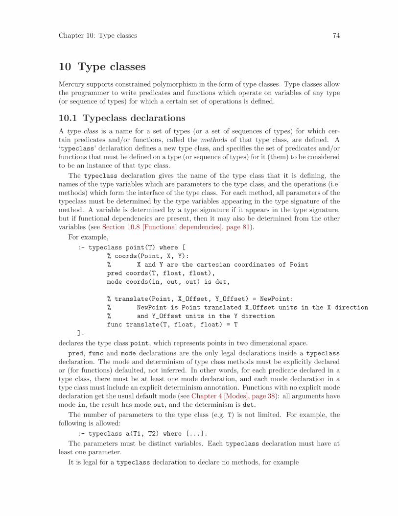
Chapter 10: Type classes 74
10 Type classes
Mercury supports constrained polymorphism in the form of type classes. Type classes allowthe programmer to write predicates and functions which operate on variables of any type(or sequence of types) for which a certain set of operations is defined.
10.1 Typeclass declarations
A type class is a name for a set of types (or a set of sequences of types) for which cer-tain predicates and/or functions, called the methods of that type class, are defined. A‘typeclass’ declaration defines a new type class, and specifies the set of predicates and/orfunctions that must be defined on a type (or sequence of types) for it (them) to be consideredto be an instance of that type class.
The typeclass declaration gives the name of the type class that it is defining, thenames of the type variables which are parameters to the type class, and the operations (i.e.methods) which form the interface of the type class. For each method, all parameters of thetypeclass must be determined by the type variables appearing in the type signature of themethod. A variable is determined by a type signature if it appears in the type signature,but if functional dependencies are present, then it may also be determined from the othervariables (see Section 10.8 [Functional dependencies], page 81).
For example,
:- typeclass point(T) where [
% coords(Point, X, Y):
% X and Y are the cartesian coordinates of Point
pred coords(T, float, float),
mode coords(in, out, out) is det,
% translate(Point, X_Offset, Y_Offset) = NewPoint:
% NewPoint is Point translated X_Offset units in the X direction
% and Y_Offset units in the Y direction
func translate(T, float, float) = T
].
declares the type class point, which represents points in two dimensional space.
pred, func and mode declarations are the only legal declarations inside a typeclass
declaration. The mode and determinism of type class methods must be explicitly declaredor (for functions) defaulted, not inferred. In other words, for each predicate declared in atype class, there must be at least one mode declaration, and each mode declaration in atype class must include an explicit determinism annotation. Functions with no explicit modedeclaration get the usual default mode (see Chapter 4 [Modes], page 38): all arguments havemode in, the result has mode out, and the determinism is det.
The number of parameters to the type class (e.g. T) is not limited. For example, thefollowing is allowed:
:- typeclass a(T1, T2) where [...].
The parameters must be distinct variables. Each typeclass declaration must have atleast one parameter.
It is legal for a typeclass declaration to declare no methods, for example
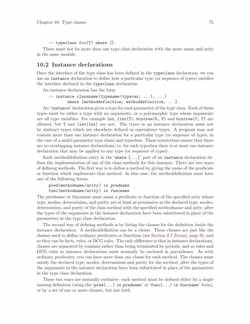
Chapter 10: Type classes 75
:- typeclass foo(T) where [].
There must not be more than one type class declaration with the same name and arityin the same module.
10.2 Instance declarations
Once the interface of the type class has been defined in the typeclass declaration, we canuse an instance declaration to define how a particular type (or sequence of types) satisfiesthe interface declared in the typeclass declaration.
An instance declaration has the form
:- instance classname(typename(typevar, ...), ...)
where [methoddefinition, methoddefinition, ...].
An ‘instance’ declaration gives a type for each parameter of the type class. Each of thesetypes must be either a type with no arguments, or a polymorphic type whose argumentsare all type variables. For example int, list(T), bintree(K, V) and bintree(T, T) areallowed, but T and list(int) are not. The types in an instance declaration must notbe abstract types which are elsewhere defined as equivalence types. A program may notcontain more than one instance declaration for a particular type (or sequence of types, inthe case of a multi-parameter type class) and typeclass. These restrictions ensure that thereare no overlapping instance declarations, i.e. for each typeclass there is at most one instancedeclaration that may be applied to any type (or sequence of types).
Each methoddefinition entry in the ‘where [...]’ part of an instance declaration de-fines the implementation of one of the class methods for this instance. There are two waysof defining methods. The first way is to define a method by giving the name of the predicateor function which implements that method. In this case, the methoddefinition must haveone of the following forms:
pred(methodname/arity) is predname
func(methodname/arity) is funcname
The predname or funcname must name a predicate or function of the specified arity whosetype, modes, determinism, and purity are at least as permissive as the declared type, modes,determinism, and purity of the class method with the specified methodname and arity, afterthe types of the arguments in the instance declaration have been substituted in place of theparameters in the type class declaration.
The second way of defining methods is by listing the clauses for the definition inside theinstance declaration. A methoddefinition can be a clause. These clauses are just like theclauses used to define ordinary predicates or functions (see Section 2.7 [Items], page 9), andso they can be facts, rules, or DCG rules. The only difference is that in instance declarations,clauses are separated by commas rather than being terminated by periods, and so rules andDCG rules in instance declarations must normally be enclosed in parentheses. As withordinary predicates, you can have more than one clause for each method. The clauses mustsatisfy the declared type, modes, determinism and purity for the method, after the types ofthe arguments in the instance declaration have been substituted in place of the parametersin the type class declaration.
These two ways are mutually exclusive: each method must be defined either by a singlenaming definition (using the ‘pred(...) is predname ’ or ‘func(...) is funcname ’ form),or by a set of one or more clauses, but not both.
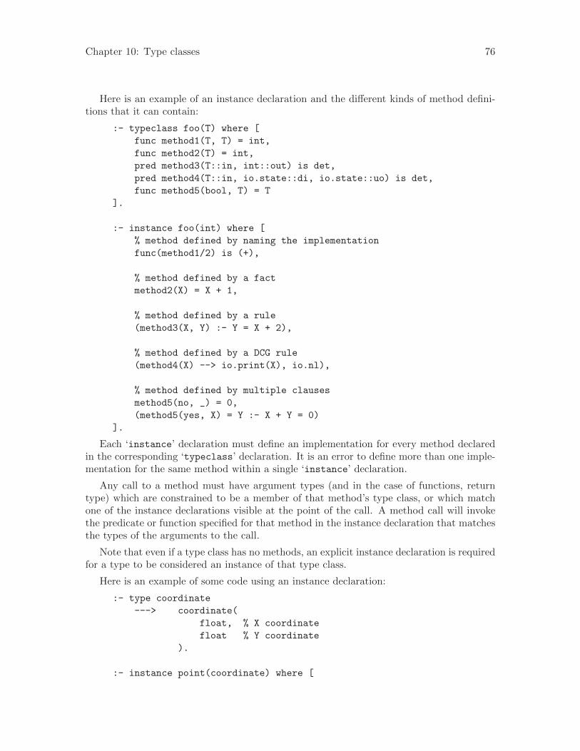
Chapter 10: Type classes 76
Here is an example of an instance declaration and the different kinds of method defini-tions that it can contain:
:- typeclass foo(T) where [
func method1(T, T) = int,
func method2(T) = int,
pred method3(T::in, int::out) is det,
pred method4(T::in, io.state::di, io.state::uo) is det,
func method5(bool, T) = T
].
:- instance foo(int) where [
% method defined by naming the implementation
func(method1/2) is (+),
% method defined by a fact
method2(X) = X + 1,
% method defined by a rule
(method3(X, Y) :- Y = X + 2),
% method defined by a DCG rule
(method4(X) --> io.print(X), io.nl),
% method defined by multiple clauses
method5(no, _) = 0,
(method5(yes, X) = Y :- X + Y = 0)
].
Each ‘instance’ declaration must define an implementation for every method declaredin the corresponding ‘typeclass’ declaration. It is an error to define more than one imple-mentation for the same method within a single ‘instance’ declaration.
Any call to a method must have argument types (and in the case of functions, returntype) which are constrained to be a member of that method’s type class, or which matchone of the instance declarations visible at the point of the call. A method call will invokethe predicate or function specified for that method in the instance declaration that matchesthe types of the arguments to the call.
Note that even if a type class has no methods, an explicit instance declaration is requiredfor a type to be considered an instance of that type class.
Here is an example of some code using an instance declaration:
:- type coordinate
---> coordinate(
float, % X coordinate
float % Y coordinate
).
:- instance point(coordinate) where [
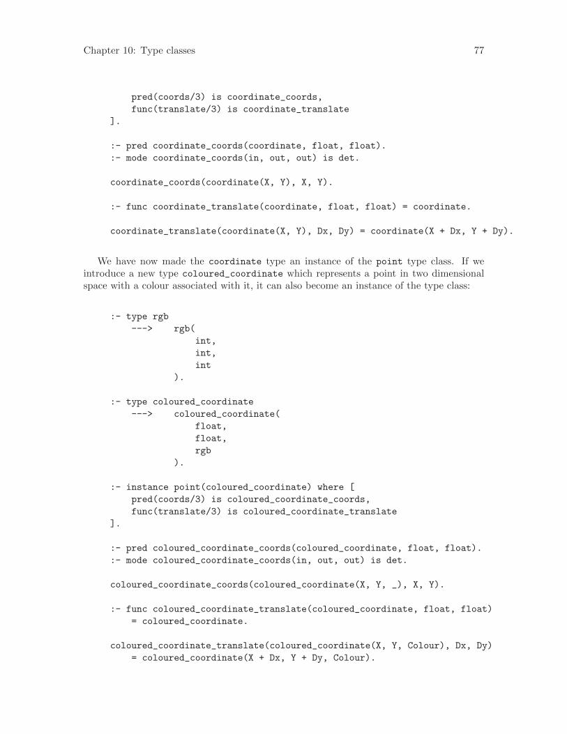
Chapter 10: Type classes 77
pred(coords/3) is coordinate_coords,
func(translate/3) is coordinate_translate
].
:- pred coordinate_coords(coordinate, float, float).
:- mode coordinate_coords(in, out, out) is det.
coordinate_coords(coordinate(X, Y), X, Y).
:- func coordinate_translate(coordinate, float, float) = coordinate.
coordinate_translate(coordinate(X, Y), Dx, Dy) = coordinate(X + Dx, Y + Dy).
We have now made the coordinate type an instance of the point type class. If weintroduce a new type coloured_coordinate which represents a point in two dimensionalspace with a colour associated with it, it can also become an instance of the type class:
:- type rgb
---> rgb(
int,
int,
int
).
:- type coloured_coordinate
---> coloured_coordinate(
float,
float,
rgb
).
:- instance point(coloured_coordinate) where [
pred(coords/3) is coloured_coordinate_coords,
func(translate/3) is coloured_coordinate_translate
].
:- pred coloured_coordinate_coords(coloured_coordinate, float, float).
:- mode coloured_coordinate_coords(in, out, out) is det.
coloured_coordinate_coords(coloured_coordinate(X, Y, _), X, Y).
:- func coloured_coordinate_translate(coloured_coordinate, float, float)
= coloured_coordinate.
coloured_coordinate_translate(coloured_coordinate(X, Y, Colour), Dx, Dy)
= coloured_coordinate(X + Dx, Y + Dy, Colour).

Chapter 10: Type classes 78
If we call ‘translate/3’ with the first argument having type ‘coloured_coordinate’,this will invoke ‘coloured_coordinate_translate’. Likewise, if we call ‘translate/3’with the first argument having type ‘coordinate’, this will invoke ‘coordinate_translate’.
Further instances of the type class could be made, e.g. a type that represents the pointusing polar coordinates.
10.3 Abstract typeclass declarations
Abstract typeclass declarations are typeclass declarations whose definitions are hidden. Anabstract typeclass declaration has the same form as a typeclass declaration, but without the‘where[...]’ part. An abstract typeclass declaration defines a name for a set of (sequencesof) types, but does not define what methods must be implemented for instances of the typeclass.
Like abstract type declarations, abstract typeclass declarations are only useful in theinterface section of a module. Each abstract typeclass declaration must be accompanied bya corresponding non-abstract typeclass declaration that defines the methods for that typeclass.
Non-abstract instance declarations can only be made in scopes where the non-abstracttypeclass declaration is visible.
10.4 Abstract instance declarations
Abstract instance declarations are instance declarations whose implementations are hidden.An abstract instance declaration has the same form as an instance declaration, but withoutthe ‘where [...]’ part. An abstract instance declaration declares that a sequence of typesis an instance of a particular type class without defining how the type class methods areimplemented for those types. Like abstract type declarations, abstract instance declarationsare only useful in the interface section of a module. Each abstract instance declaration mustbe accompanied by a corresponding non-abstract instance declaration that defines how thetype class methods are implemented.
Here is an example:
:- module hashable.
:- interface.
:- import_module int, string.
:- typeclass hashable(T) where [func hash(T) = int].
:- instance hashable(int).
:- instance hashable(string).
:- implementation.
:- instance hashable(int) where [func(hash/1) is hash_int].
:- instance hashable(string) where [func(hash/1) is hash_string].
:- func hash_int(int) = int.
hash_int(X) = X.

Chapter 10: Type classes 79
:- func hash_string(string) = int.
hash_string(S) = H :-
% Use the standard library predicate string.hash/2.
string.hash(S, H).
:- end_module hashable.
10.5 Type class constraints on predicates and functions
Mercury allows a type class constraint to appear as part of a predicate or function’s typesignature. This constrains the values that can be taken by type variables in the signatureto belong to particular type classes.
A type class constraint has the form:
<= Typeclass(Type, ...), ...
where Typeclass is the name of a type class and Type is a type. Any variable that appearsin Type must be determined by the predicate’s or function’s type signature. A variable isdetermined by a type signature if it appears in the type signature, but if functional depen-dencies are present, then it may also be determined from other variables (see Section 10.8[Functional dependencies], page 81). Each type class constraint in a predicate or functiondeclaration must contain at least one variable.
For example
:- pred distance(P1, P2, float) <= (point(P1), point(P2)).
:- mode distance(in, in, out) is det.
distance(A, B, Distance) :-
coords(A, Xa, Ya),
coords(B, Xb, Yb),
XDist = Xa - Xb,
YDist = Ya - Yb,
Distance = sqrt(XDist*XDist + YDist*YDist).
In the above example, the distance predicate is able to calculate the distance betweenany two points, regardless of their representation, as long as the coords operation has beendefined. These constraints are checked at compile time.
10.6 Type class constraints on type class declarations
Type class constraints may also appear in typeclass declarations, meaning that one typeclass is a “superclass” of another.
The arguments of a constraint on a type class declaration must be either type variables orground types. Each constraint must contain at least one variable argument and all variablesthat appear in the arguments must also be arguments to the type class in question.
For example, the following declares the ‘ring’ type class, which describes types with aparticular set of numerical operations defined:
:- typeclass ring(T) where [
func zero = (T::out) is det, % ’+’ identity
func one = (T::out) is det, % ’*’ identity

Chapter 10: Type classes 80
func plus(T::in, T::in) = (T::out) is det, % ’+’/2 (forward mode)
func mult(T::in, T::in) = (T::out) is det, % ’*’/2 (forward mode)
func negative(T::in) = (T::out) is det % ’-’/1 (forward mode)
].
We can now add the following declaration:
:- typeclass euclidean(T) <= ring(T) where [
func div(T::in, T::in) = (T::out) is det,
func mod(T::in, T::in) = (T::out) is det
].
This introduces a new type class, euclidean, of which ring is a superclass. The opera-tions defined by the euclidean type class are div, mod, as well as all those defined by thering type class. Any type declared to be an instance of euclidean must also be declaredto be an instance of ring.
Type class constraints on type class declarations gives rise to a superclass relation. Thisrelation must be acyclic. That is, it is an error if a type class is its own (direct or indirect)superclass.
10.7 Type class constraints on instance declarations
Type class constraints may also be placed upon instance declarations. The argumentsof such constraints must be either type variables or ground types. Each constraint mustcontain at least one variable argument and all variables that appear in the arguments mustbe type variables that appear in the types in the instance declaration.
For example, consider the following declaration of a type class of types that may beprinted:
:- typeclass portrayable(T) where [
pred portray(T::in, io.state::di, io.state::uo) is det
].
The programmer could declare instances such as
:- instance portrayable(int) where [
pred(portray/3) is io.write_int
].
:- instance portrayable(char) where [
pred(portray/3) is io.write_char
].
However, when it comes to writing the instance declaration for a type such as list(T),we want to be able print out the list elements using the portray/3 for the particular type ofthe list elements. This can be achieved by placing a type class constraint on the instancedeclaration, as in the following example:
:- instance portrayable(list(T)) <= portrayable(T) where [
pred(portray/3) is portray_list
].
:- pred portray_list(list(T), io.state, io.state) <= portrayable(T).
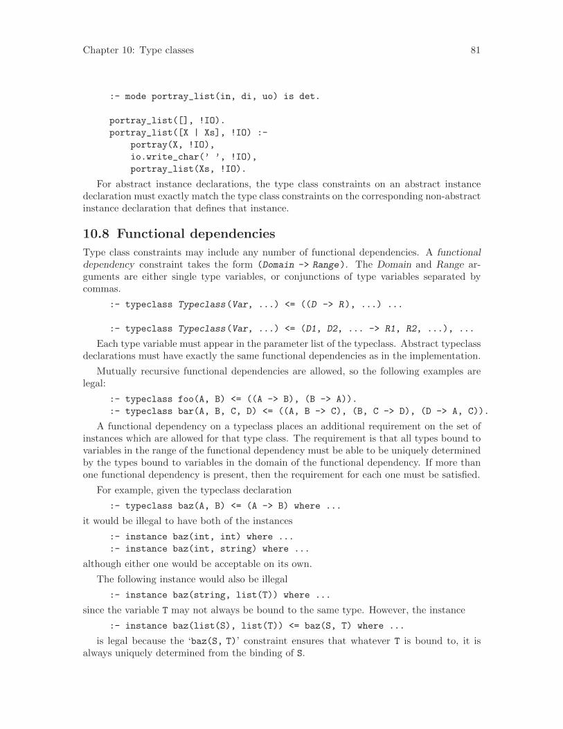
Chapter 10: Type classes 81
:- mode portray_list(in, di, uo) is det.
portray_list([], !IO).
portray_list([X | Xs], !IO) :-
portray(X, !IO),
io.write_char(’ ’, !IO),
portray_list(Xs, !IO).
For abstract instance declarations, the type class constraints on an abstract instancedeclaration must exactly match the type class constraints on the corresponding non-abstractinstance declaration that defines that instance.
10.8 Functional dependencies
Type class constraints may include any number of functional dependencies. A functionaldependency constraint takes the form (Domain -> Range). The Domain and Range ar-guments are either single type variables, or conjunctions of type variables separated bycommas.
:- typeclass Typeclass(Var, ...) <= ((D -> R), ...) ...
:- typeclass Typeclass(Var, ...) <= (D1, D2, ... -> R1, R2, ...), ...
Each type variable must appear in the parameter list of the typeclass. Abstract typeclassdeclarations must have exactly the same functional dependencies as in the implementation.
Mutually recursive functional dependencies are allowed, so the following examples arelegal:
:- typeclass foo(A, B) <= ((A -> B), (B -> A)).
:- typeclass bar(A, B, C, D) <= ((A, B -> C), (B, C -> D), (D -> A, C)).
A functional dependency on a typeclass places an additional requirement on the set ofinstances which are allowed for that type class. The requirement is that all types bound tovariables in the range of the functional dependency must be able to be uniquely determinedby the types bound to variables in the domain of the functional dependency. If more thanone functional dependency is present, then the requirement for each one must be satisfied.
For example, given the typeclass declaration
:- typeclass baz(A, B) <= (A -> B) where ...
it would be illegal to have both of the instances
:- instance baz(int, int) where ...
:- instance baz(int, string) where ...
although either one would be acceptable on its own.
The following instance would also be illegal
:- instance baz(string, list(T)) where ...
since the variable T may not always be bound to the same type. However, the instance
:- instance baz(list(S), list(T)) <= baz(S, T) where ...
is legal because the ‘baz(S, T)’ constraint ensures that whatever T is bound to, it isalways uniquely determined from the binding of S.

Chapter 10: Type classes 82
The extra requirements that result from the use of functional dependencies allow thebindings of some variables to be determined from the bindings of others. This in turn relaxessome of the requirements of typeclass constraints on predicate and function signatures, andon existentially typed data constructors.
Without any functional dependencies, all variables in constraints must appear in thesignature of the predicate or function being declared. However, variables which are in therange of a functional dependency need not appear in the signature, since it is known thattheir bindings will be determined from the bindings of the variables in the domain.
More formally, the constraints on a predicate or function signature induce a set of func-tional dependencies on the variables appearing in those constraints. A functional depen-dency ‘(A1, ... -> B1, ...)’ is induced from a constraint ‘Typeclass(Type1, ...)’ ifand only if the typeclass ‘Typeclass ’ has a functional dependency ‘(D1, ... -> R1, ...)’,and for each typeclass parameter ‘Di’ there exists an ‘Aj’ every type variable appearingin the ‘Typek ’ corresponding to ‘Di’, and each ‘Bi’ appears in the ‘Typej ’ bound to thetypeclass parameter ‘Rk’ for some k.
For example, with the definition of baz above, the constraint baz(map(X, Y), list(Z))
induces the constraint (X, Y -> Z), since X and Y appear in the domain argument, and Zappears in the range argument.
The set of type variables determined from a signature is the closure of the set appearing inthe signature under the functional dependencies induced from the constraints. The closureis defined as the smallest set of variables which includes all of the variables appearing in thesignature, and is such that, for each induced functional dependency ‘Domain -> Range ’, ifthe closure includes all of the variables in Domain then it includes all of the variables inRange.
For example, the declaration
:- pred p(X, Y) <= baz(map(X, Y), list(Z)).
is acceptable since the closure of {X, Y} under the induced functional dependency mustinclude Z. Moreover, the typeclass baz/2 would be allowed to have a method that only usesthe first parameter, A, since the second parameter, B, would always be determined fromthe first.
Note that, since all instances must satisfy the superclass constraints, the restrictions oninstances obviously transfer from superclass to subclass. Again, this allows the requirementsof typeclass constraints to be relaxed. Thus, the functional dependencies on the ancestorsof constraints also induce functional dependencies on the variables, and the closure that wecalculate takes these into account.
For example, in this code
:- typeclass quux(P, Q, R) <= baz(R, P) where ...
:- pred q(Q, R) <= quux(P, Q, R).
the signature of q/2 is acceptable since the superclass constraint on quux/2 induces thedependency ‘R -> P’ on the type variables, hence P is in the closure of {Q, R}.
The presence of functional dependencies also allows “improvement” to occur duringtype inference. This can occur in two ways. First, if two constraints of a given class matchon all of the domain arguments of a functional dependency on that class, then it can be

Chapter 10: Type classes 83
inferred that they also match on the range arguments. For example, given the constraintsbaz(A, B1) and baz(A, B2), it will be inferred that B1 = B2.
Similarly, if a constraint of a given class is subsumed by a known instance of that classin the domain arguments, then its range arguments can be unified with the correspondinginstance range arguments. For example, given the instance:
:- instance baz(list(T), string) where ...
then the constraint baz(list(int), X) can be improved with the inference thatX = string.

Chapter 11: Existential types 84
11 Existential types
Existentially quantified type variables (or simply “existential types” for short) are usefultools for data abstraction. In combination with type classes, they allow you to write codein an “object oriented” style that is similar to the use of interfaces in Java or abstract baseclasses in C++.
Mercury supports existential type quantifiers on predicate and function declarations,and in data type definitions. You can put type class constraints on existentially quantifiedtype variables.
11.1 Existentially typed predicates and functions
11.1.1 Syntax for explicit type quantifiers
Type variables in type declarations for polymorphic predicates or functions are normallyuniversally quantified. However, it is also possible to existentially quantify such type vari-ables, by using an explicit existential quantifier of the form ‘some Vars ’ before the ‘pred’or ‘func’ declaration, where Vars is a list of variables.
For example:
% Here the type variables ‘T’ is existentially quantified
:- some [T] pred foo(T).
% Here the type variables ‘T1’ and ‘T2’ are existentially quantified.
:- some [T1, T2] func bar(int, list(T1), set(T2)) = pair(T1, T2).
% Here the type variable ‘T2’ is existentially quantified,
% but the type variables ‘T1’ and ‘T3’ are universally quantified.
:- some [T2] pred foo(T1, T2, T3).
Explicit universal quantifiers, of the form ‘all Vars ’, are also permitted on ‘pred’ and‘func’ declarations, although they are not necessary, since universal quantification is thedefault. (If both universal and existential quantifiers are present, the universal quantifiersmust precede the existential quantifiers.) For example:
% Here the type variable ‘T2’ is existentially quantified,
% but the type variables ‘T1’ and ‘T3’ are universally quantified.
:- all [T3] some [T2] pred foo(T1, T2, T3).
11.1.2 Semantics of type quantifiers
If a type variable in the type declaration for a polymorphic predicate or function is univer-sally quantified, this means the caller will determine the value of the type variable, and thecallee must be defined so that it will work for all types which are an instance of its declaredtype.
For an existentially quantified type variable, the situation is the converse: the calleemust determine the value of the type variable, and all callers must be defined so as to workfor all types which are an instance of the called procedure’s declared type.
When type checking a predicate or function, if a variable has a type that occurs as auniversally quantified type variable in the predicate or function declaration, or a type that
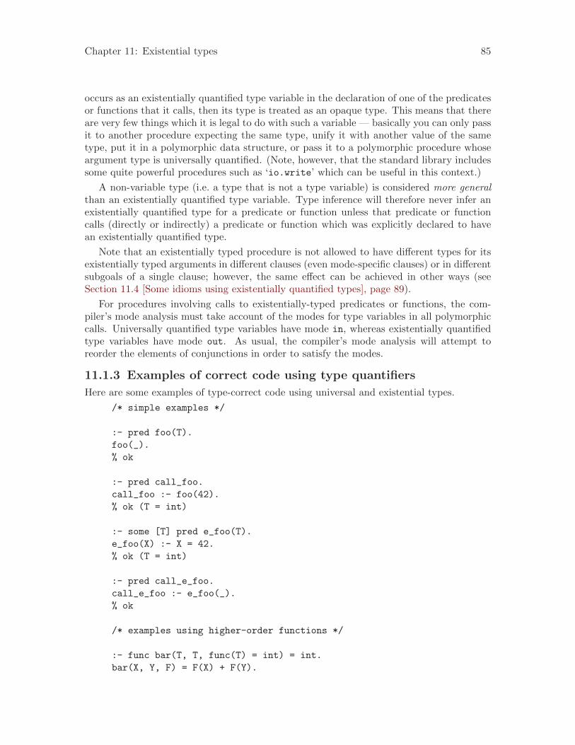
Chapter 11: Existential types 85
occurs as an existentially quantified type variable in the declaration of one of the predicatesor functions that it calls, then its type is treated as an opaque type. This means that thereare very few things which it is legal to do with such a variable — basically you can only passit to another procedure expecting the same type, unify it with another value of the sametype, put it in a polymorphic data structure, or pass it to a polymorphic procedure whoseargument type is universally quantified. (Note, however, that the standard library includessome quite powerful procedures such as ‘io.write’ which can be useful in this context.)
A non-variable type (i.e. a type that is not a type variable) is considered more generalthan an existentially quantified type variable. Type inference will therefore never infer anexistentially quantified type for a predicate or function unless that predicate or functioncalls (directly or indirectly) a predicate or function which was explicitly declared to havean existentially quantified type.
Note that an existentially typed procedure is not allowed to have different types for itsexistentially typed arguments in different clauses (even mode-specific clauses) or in differentsubgoals of a single clause; however, the same effect can be achieved in other ways (seeSection 11.4 [Some idioms using existentially quantified types], page 89).
For procedures involving calls to existentially-typed predicates or functions, the com-piler’s mode analysis must take account of the modes for type variables in all polymorphiccalls. Universally quantified type variables have mode in, whereas existentially quantifiedtype variables have mode out. As usual, the compiler’s mode analysis will attempt toreorder the elements of conjunctions in order to satisfy the modes.
11.1.3 Examples of correct code using type quantifiers
Here are some examples of type-correct code using universal and existential types.
/* simple examples */
:- pred foo(T).
foo(_).
% ok
:- pred call_foo.
call_foo :- foo(42).
% ok (T = int)
:- some [T] pred e_foo(T).
e_foo(X) :- X = 42.
% ok (T = int)
:- pred call_e_foo.
call_e_foo :- e_foo(_).
% ok
/* examples using higher-order functions */
:- func bar(T, T, func(T) = int) = int.
bar(X, Y, F) = F(X) + F(Y).
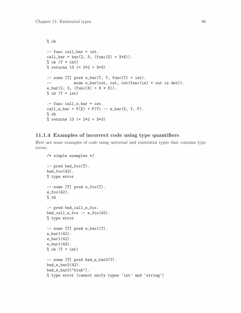
Chapter 11: Existential types 86
% ok
:- func call_bar = int.
call_bar = bar(2, 3, (func(X) = X*X)).
% ok (T = int)
% returns 13 (= 2*2 + 3*3)
:- some [T] pred e_bar(T, T, func(T) = int).
:- mode e_bar(out, out, out(func(in) = out is det)).
e_bar(2, 3, (func(X) = X * X)).
% ok (T = int)
:- func call_e_bar = int.
call_e_bar = F(X) + F(Y) :- e_bar(X, Y, F).
% ok
% returns 13 (= 2*2 + 3*3)
11.1.4 Examples of incorrect code using type quantifiers
Here are some examples of code using universal and existential types that contains typeerrors.
/* simple examples */
:- pred bad_foo(T).
bad_foo(42).
% type error
:- some [T] pred e_foo(T).
e_foo(42).
% ok
:- pred bad_call_e_foo.
bad_call_e_foo :- e_foo(42).
% type error
:- some [T] pred e_bar1(T).
e_bar1(42).
e_bar1(42).
e_bar1(43).
% ok (T = int)
:- some [T] pred bad_e_bar2(T).
bad_e_bar2(42).
bad_e_bar2("blah").
% type error (cannot unify types ‘int’ and ‘string’)
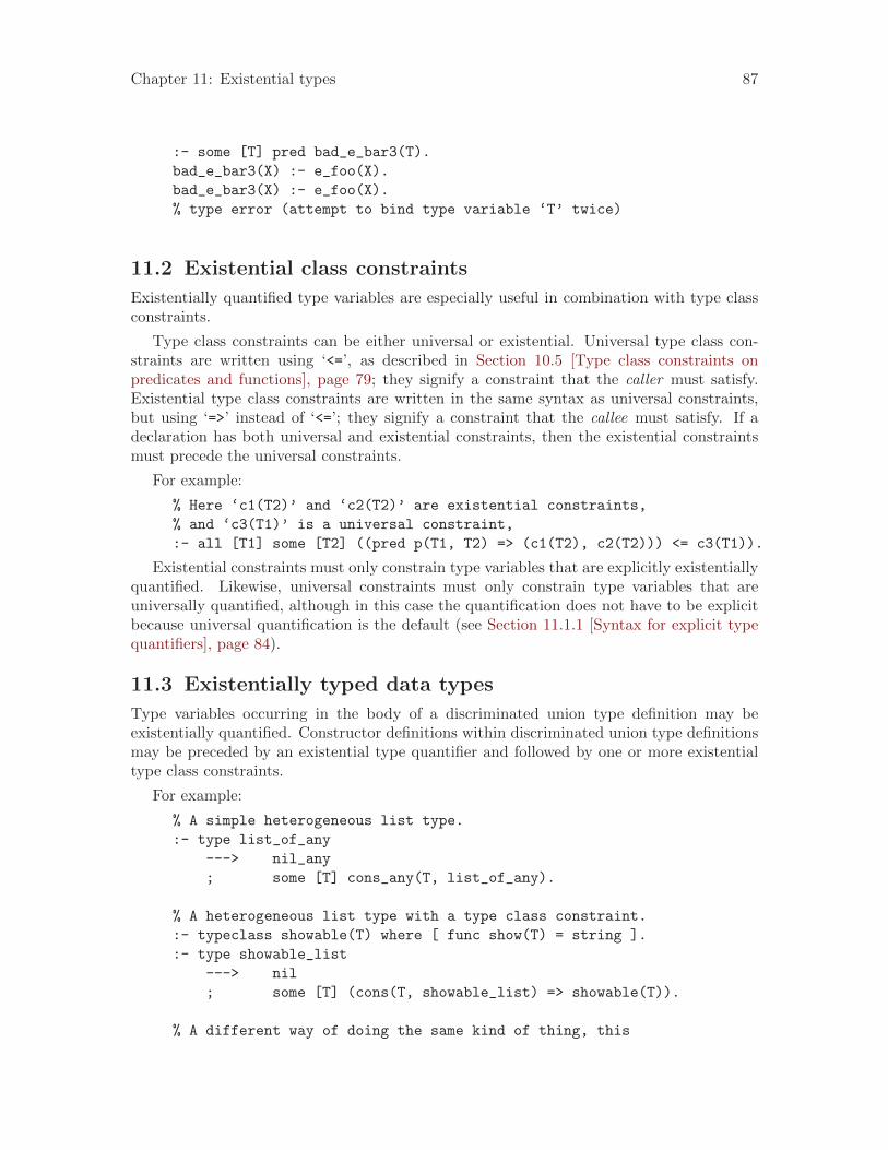
Chapter 11: Existential types 87
:- some [T] pred bad_e_bar3(T).
bad_e_bar3(X) :- e_foo(X).
bad_e_bar3(X) :- e_foo(X).
% type error (attempt to bind type variable ‘T’ twice)
11.2 Existential class constraints
Existentially quantified type variables are especially useful in combination with type classconstraints.
Type class constraints can be either universal or existential. Universal type class con-straints are written using ‘<=’, as described in Section 10.5 [Type class constraints onpredicates and functions], page 79; they signify a constraint that the caller must satisfy.Existential type class constraints are written in the same syntax as universal constraints,but using ‘=>’ instead of ‘<=’; they signify a constraint that the callee must satisfy. If adeclaration has both universal and existential constraints, then the existential constraintsmust precede the universal constraints.
For example:
% Here ‘c1(T2)’ and ‘c2(T2)’ are existential constraints,
% and ‘c3(T1)’ is a universal constraint,
:- all [T1] some [T2] ((pred p(T1, T2) => (c1(T2), c2(T2))) <= c3(T1)).
Existential constraints must only constrain type variables that are explicitly existentiallyquantified. Likewise, universal constraints must only constrain type variables that areuniversally quantified, although in this case the quantification does not have to be explicitbecause universal quantification is the default (see Section 11.1.1 [Syntax for explicit typequantifiers], page 84).
11.3 Existentially typed data types
Type variables occurring in the body of a discriminated union type definition may beexistentially quantified. Constructor definitions within discriminated union type definitionsmay be preceded by an existential type quantifier and followed by one or more existentialtype class constraints.
For example:
% A simple heterogeneous list type.
:- type list_of_any
---> nil_any
; some [T] cons_any(T, list_of_any).
% A heterogeneous list type with a type class constraint.
:- typeclass showable(T) where [ func show(T) = string ].
:- type showable_list
---> nil
; some [T] (cons(T, showable_list) => showable(T)).
% A different way of doing the same kind of thing, this
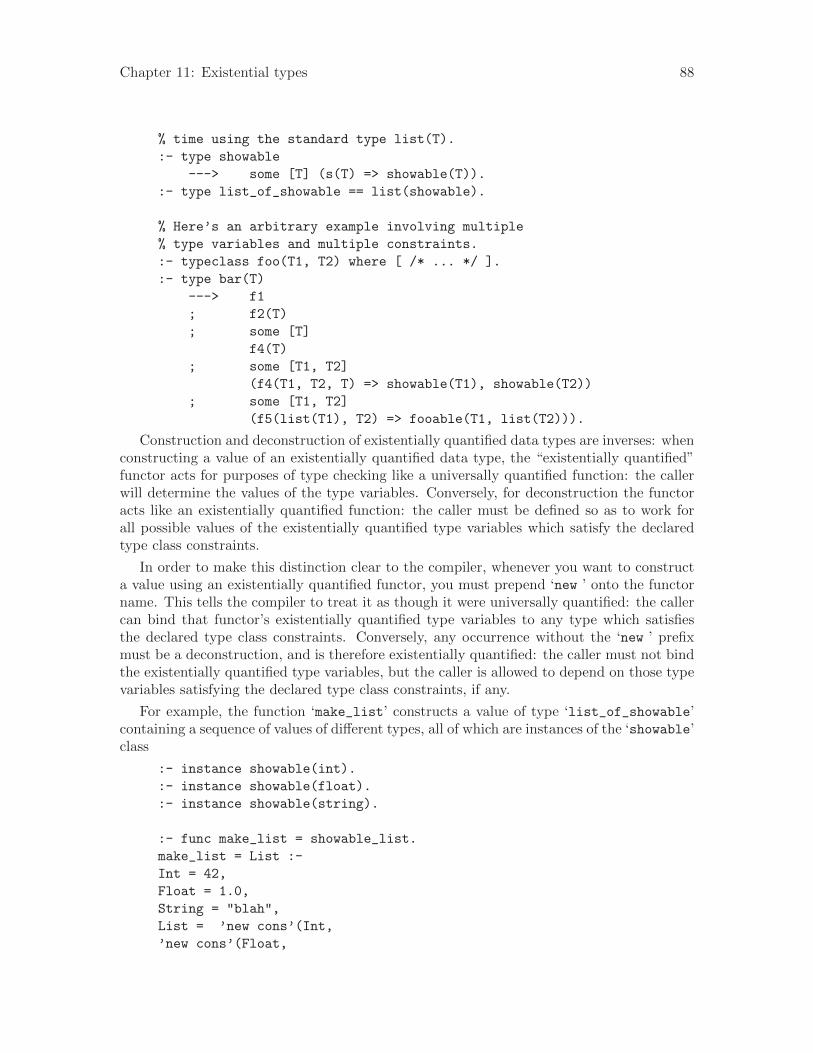
Chapter 11: Existential types 88
% time using the standard type list(T).
:- type showable
---> some [T] (s(T) => showable(T)).
:- type list_of_showable == list(showable).
% Here’s an arbitrary example involving multiple
% type variables and multiple constraints.
:- typeclass foo(T1, T2) where [ /* ... */ ].
:- type bar(T)
---> f1
; f2(T)
; some [T]
f4(T)
; some [T1, T2]
(f4(T1, T2, T) => showable(T1), showable(T2))
; some [T1, T2]
(f5(list(T1), T2) => fooable(T1, list(T2))).
Construction and deconstruction of existentially quantified data types are inverses: whenconstructing a value of an existentially quantified data type, the “existentially quantified”functor acts for purposes of type checking like a universally quantified function: the callerwill determine the values of the type variables. Conversely, for deconstruction the functoracts like an existentially quantified function: the caller must be defined so as to work forall possible values of the existentially quantified type variables which satisfy the declaredtype class constraints.
In order to make this distinction clear to the compiler, whenever you want to constructa value using an existentially quantified functor, you must prepend ‘new ’ onto the functorname. This tells the compiler to treat it as though it were universally quantified: the callercan bind that functor’s existentially quantified type variables to any type which satisfiesthe declared type class constraints. Conversely, any occurrence without the ‘new ’ prefixmust be a deconstruction, and is therefore existentially quantified: the caller must not bindthe existentially quantified type variables, but the caller is allowed to depend on those typevariables satisfying the declared type class constraints, if any.
For example, the function ‘make_list’ constructs a value of type ‘list_of_showable’containing a sequence of values of different types, all of which are instances of the ‘showable’class
:- instance showable(int).
:- instance showable(float).
:- instance showable(string).
:- func make_list = showable_list.
make_list = List :-
Int = 42,
Float = 1.0,
String = "blah",
List = ’new cons’(Int,
’new cons’(Float,
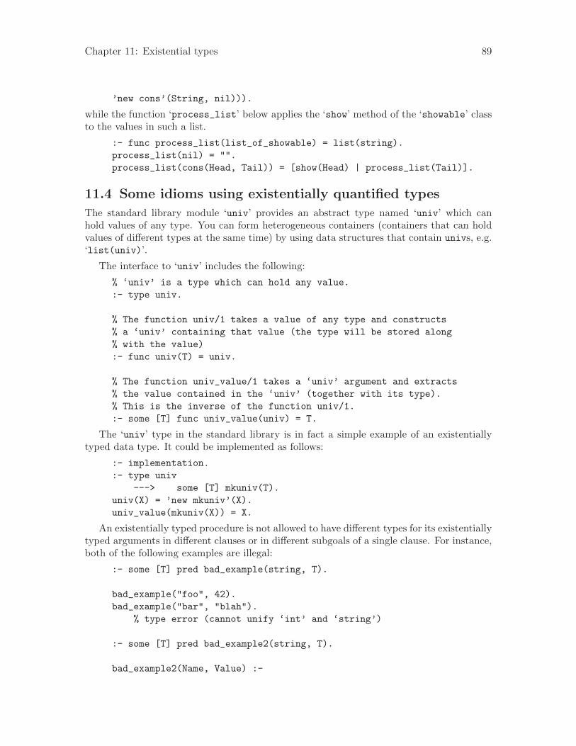
Chapter 11: Existential types 89
’new cons’(String, nil))).
while the function ‘process_list’ below applies the ‘show’ method of the ‘showable’ classto the values in such a list.
:- func process_list(list_of_showable) = list(string).
process_list(nil) = "".
process_list(cons(Head, Tail)) = [show(Head) | process_list(Tail)].
11.4 Some idioms using existentially quantified types
The standard library module ‘univ’ provides an abstract type named ‘univ’ which canhold values of any type. You can form heterogeneous containers (containers that can holdvalues of different types at the same time) by using data structures that contain univs, e.g.‘list(univ)’.
The interface to ‘univ’ includes the following:
% ‘univ’ is a type which can hold any value.
:- type univ.
% The function univ/1 takes a value of any type and constructs
% a ‘univ’ containing that value (the type will be stored along
% with the value)
:- func univ(T) = univ.
% The function univ_value/1 takes a ‘univ’ argument and extracts
% the value contained in the ‘univ’ (together with its type).
% This is the inverse of the function univ/1.
:- some [T] func univ_value(univ) = T.
The ‘univ’ type in the standard library is in fact a simple example of an existentiallytyped data type. It could be implemented as follows:
:- implementation.
:- type univ
---> some [T] mkuniv(T).
univ(X) = ’new mkuniv’(X).
univ_value(mkuniv(X)) = X.
An existentially typed procedure is not allowed to have different types for its existentiallytyped arguments in different clauses or in different subgoals of a single clause. For instance,both of the following examples are illegal:
:- some [T] pred bad_example(string, T).
bad_example("foo", 42).
bad_example("bar", "blah").
% type error (cannot unify ‘int’ and ‘string’)
:- some [T] pred bad_example2(string, T).
bad_example2(Name, Value) :-

Chapter 11: Existential types 90
( Name = "foo", Value = 42
; Name = "bar", Value = "blah"
).
% type error (cannot unify ‘int’ and ‘string’)
However, using ‘univ’, it is possible for an existentially typed function to return valuesof different types at each invocation.
:- some [T] pred good_example(string, T).
good_example(Name, univ_value(Univ)) :-
( Name = "foo", Univ = univ(42)
; Name = "bar", Univ = univ("blah")
).
Using ‘univ’ doesn’t work if you also want to use type class constraints. If you wantto use type class constraints, then you must define your own existentially typed data type,analogous to ‘univ’, and use that:
:- type univ_showable
---> some [T] (mkshowable(T) => showable(T)).
:- some [T] pred harder_example(string, T) => showable(T).
harder_example(Name, Showable) :-
( Name = "bar", Univ = ’new mkshowable’(42)
; Name = "bar", Univ = ’new mkshowable’("blah")
),
Univ = mkshowable(Showable).
The issue can also arise for mode-specific clauses (see Section 4.4 [Different clauses fordifferent modes], page 44). For instance, the following example is illegal:
:- some [T] pred bad_example3(string, T).
:- mode bad_example3(in(bound("foo")), out) is det.
:- mode bad_example3(in(bound("bar")), out) is det.
:- pragma promise_pure(bad_example3/2).
bad_example3("foo"::in(bound("foo")), 42::out).
bad_example3("bar"::in(bound("bar")), "blah"::out).
% type error (cannot unify ‘int’ and ‘string’)
The solution is similar, although in this case an intermediate predicate is required:
:- some [T] pred good_example3(string, T).
:- mode good_example3(in(bound("foo")), out) is det.
:- mode good_example3(in(bound("bar")), out) is det.
good_example3(Name, univ_value(Univ)) :-
good_example3_univ(Name, Univ).
:- pred good_example3_univ(string, univ).
:- mode good_example3_univ(in(bound("foo")), out) is det.
:- mode good_example3_univ(in(bound("bar")), out) is det.
:- pragma promise_pure(good_example3_univ/2).
Chapter 11: Existential types 91
good_example3_univ("foo"::in(bound("foo")), univ(42)::out).
good_example3_univ("bar"::in(bound("bar")), univ("blah")::out).

Chapter 12: Exception handling 92
12 Exception handling
Mercury procedures may throw exceptions. Exceptions may be caught using the predicatesdefined in the ‘exception’ library module, or using try goals.
A ‘try’ goal has the following form:
try Params Goal
then ThenGoal
else ElseGoal
catch Term -> CatchGoal
...
catch_any CatchAnyVar -> CatchAnyGoal
Goal, ThenGoal, ElseGoal, CatchGoal, CatchAnyGoal must be valid goals.
Goal must have one of the following determinisms: det, semidet, cc_multi, orcc_nondet.
The non-local variables of Goal must not have an inst equivalent to unique,mostly_unique or any, unless they have the type ‘io.state’.
Params must be a valid list of zero or more try parameters.
The “then” part is mandatory. The “else” part is mandatory if Goal may fail; otherwiseit must be omitted. There may be zero or more “catch” branches. The “catch any” part isoptional. CatchAnyVar must be a single variable.
The try parameter ‘io’ takes a single argument, which must be the name of a statevariable prefixed by ‘!’; for example, ‘io(!IO)’. The state variable must have the type‘io.state’, and be in scope of the try goal. The state variable is threaded through Goal,so it may perform I/O but cannot fail. If no ‘io’ parameter exists, Goal may not performI/O and may fail.
A try goal has determinism cc_multi.
On entering a try goal, Goal is executed. If it succeeds without throwing an exception,ThenGoal is executed. Any variables bound by Goal are visible in ThenGoal only. If Goalfails, then ElseGoal is executed.
If Goal throws an exception, the exception value is unified with each of the Terms in the“catch” branches in turn. On the first successful unification, the corresponding CatchGoalis executed (and other “catch” and “catch any” branches ignored). Variables bound duringthe unification of the Term are in scope of the corresponding CatchGoal.
If the exception value does not unify with any of the terms in “catch” branches, and a“catch any” branch is present, the exception is bound to CatchAnyVar and the CatchAny-Goal executed. CatchAnyVar is visible in the CatchAnyGoal only, and is existentiallytyped, i.e. it has type ‘some [T] T’.
Finally, if the thrown value did not unify with any “catch” term, and there is no“catch any” branch, the exception is rethrown.
The declarative semantics of a try goal is:

Chapter 12: Exception handling 93
(
try [] Goal
then Then
else Else
catch CP1 -> CG1
catch CP2 -> CG2
...
catch_any CAV -> CAG
)
<=>
(
Goal, Then
;
not Goal, Else
;
some [Excp]
( if Excp = CP1 then
CG1
else if Excp = CP2 then
CG2
else if ...
...
else
Excp = CAV,
CAG
)
).
If no ‘else’ branch is present, then ‘Else = fail’. If no ‘catch_any’ branch is present,then ‘CAG = fail’.
An example of a try goal that performs I/O is:
:- pred p_carefully(io::di, io::uo) is cc_multi.
p_carefully(!IO) :-
(try [io(!IO)] (
io.write_string("Calling p\n", !IO),
p(Output, !IO)
)
then
io.write_string("p returned: ", !IO),
io.write(Output, !IO),
io.nl(!IO)
catch S ->
io.write_string("p threw a string: ", !IO),
io.write_string(S, !IO),
io.nl(!IO)
catch 42 ->
Chapter 12: Exception handling 94
io.write_string("p threw 42\n", !IO)
catch_any Other ->
io.write_string("p threw something: ", !IO),
io.write(Other, !IO),
% Rethrow the value.
throw(Other)
).

Chapter 13: Semantics 95
13 Semantics
A legal Mercury program is one that complies with the syntax, type, mode, determinism,and module system rules specified in earlier chapters. If a program does not comply withthose rules, the compiler must report an error.
For each legal Mercury program, there is an associated predicate calculus theory whoselanguage is specified by the type declarations in the program and whose axioms are thecompletion of the clauses for all predicates in the program, plus the usual equality axiomsextended with the completion of the equations for all functions in the program, plus axiomscorresponding to the mode-determinism assertions (see Chapter 6 [Determinism], page 48),plus axioms specifying the semantics of library predicates and functions. The declarativesemantics of a legal Mercury program is specified by this theory.
Mercury implementations must be sound: the answers they compute must be true inevery model of the theory. Mercury implementations are not required to be complete: theymay fail to compute an answer in finite time, or they may exhaust the resource limitations ofthe execution environment, even though an answer is provable in the theory. However, thereare certain minimum requirements that they must satisfy with respect to completeness.
There is an operational semantics of Mercury programs called the strict sequential op-erational semantics. In this semantics, the program is executed top-down, starting from‘main/2’ preceded by any module initialisation goals (as per Section 9.4 [Module initial-isation], page 70), followed by any module finalisation goals (as per Section 9.5 [Modulefinalisation], page 71), and function calls within a goal, conjunctions and disjunctions areall executed in depth-first left-to-right order. Conjunctions and function calls are “mini-mally” reordered as required by the modes: the order is determined by selecting the firstmode-correct sub-goal (conjunct or function call), executing that, then selecting the firstof the remaining sub-goals which is now mode-correct, executing that, and so on. (Thereis no interleaving of different individual conjuncts or function calls, however; the sub-goalsare reordered, not split and interleaved.) Function application is strict, not lazy.
Mercury implementations are required to provide a method of processing Mercury pro-grams which is equivalent to the strict sequential operational semantics.
There is another operational semantics of Mercury programs called the strict commuta-tive operational semantics. This semantics is equivalent to the strict sequential operationalsemantics except that there is no requirement that function calls, conjunctions and dis-junctions be executed left-to-right; they may be executed in any order, and may even beinterleaved. Furthermore, the order may even be different each time a particular goal isentered.
As well as providing the strict sequential operational semantics, Mercury implementa-tions may optionally provide additional implementation-defined operational semantics, pro-vided that any such implementation-defined operational semantics are at least as completeas the strict commutative operational semantics. An implementation-defined semantics is“at least as complete” as the strict commutative semantics if and only if the implementation-defined semantics guarantees to compute an answer in finite time for any program for whichan answer would be computed in finite time for all possible executions under the strict com-mutative semantics (i.e. for all possible orderings of conjunctions and disjunctions).
Thus, to summarize, there are in fact a variety of different operational semantics forMercury. In one of them, the strict sequential semantics, there is no nondeterminism —
Chapter 13: Semantics 96
the behaviour is always specified exactly. Programs are executed top-down using SLDNF(or something equivalent), mode analysis does “minimal” reordering (in a precisely definedsense), function calls, conjunctions and disjunctions are executed depth-first left-to-right,and function evaluation is strict. All implementations are required to support the strictsequential semantics, so that a program which works on one implementation using this se-mantics will be guaranteed to work on any other implementation. However, implementationsare also allowed to support other operational semantics, which may have non-determinism,so long as they are sound with respect to the declarative semantics, and so long as theymeet a minimum level of completeness (they must be at least as complete as the strictcommutative semantics, in the sense that every program which terminates for all possibleorderings must also terminate in any implementation-defined operational semantics).
This compromise allows Mercury to be used in several different ways. Programmers whocare more about ease of programming and portability than about efficiency can use the strictsequential semantics, and can then be guaranteed that if their program works on one correctimplementation, it will work on all correct implementations. Compiler implementors whowant to write optimizing implementations that do lots of clever code reorderings and otherhigh-level transformations or that want to offer parallelizing implementations which takemaximum advantage of parallelism can define different semantic models. Programmers whocare about efficiency more than portability can write code for these implementation-definedsemantic models. Programmers who care about efficiency and portability can achieve thisby writing code for the strict commutative semantics. Of course, this is not quite as easyas using the strict sequential semantics, since it is in general not sufficient to test yourprograms on just one implementation if you are to be sure that it will be able to use themaximally efficient operational semantics on any implementation. However, if you do writecode which works for all possible executions under the strict commutative semantics (i.e. forall possible orderings of conjunctions and disjunctions), then you can be guaranteed that itwill work correctly on every implementation, under every possible implementation-definedsemantics.
The Melbourne Mercury implementation offers eight different semantics, which can beselected with different combinations of the ‘--no-reorder-conj’, ‘--no-reorder-disj’,and ‘--no-fully-strict’ options. (The ‘--no-fully-strict’ option allows the com-piler to improve completeness by optimizing away infinite loops and goals with determin-ism erroneous.) The default semantics are the strict commutative semantics. Enabling‘--no-reorder-conj’ and ‘--no-reorder-disj’ gives the strict sequential semantics.
Future implementations of Mercury may wish to offer other operational semantics. Forexample, they may wish to provide semantics in which function evaluation is lazy, ratherthan strict; semantics with a guaranteed fair search rule; and so forth.

Chapter 14: Foreign language interface 97
14 Foreign language interface
This chapter documents the foreign language interface.
14.1 Calling foreign code from Mercury
Mercury procedures can be implemented using fragments of foreign language code using‘pragma foreign_proc’.
14.1.1 pragma foreign proc
A declaration of the form
:- pragma foreign_proc("Lang",
Pred(Var1::Mode1, Var2::Mode2, ...),
Attributes, Foreign_Code).
or
:- pragma foreign_proc("Lang",
Func(Var1::Mode1, Var2::Mode2, ...) = (Var::Mode),
Attributes, Foreign_Code).
means that any calls to the specified mode of Pred or Func will result in execution ofthe foreign code given in Foreign Code written in language Lang, if Lang is selected asthe foreign language code by this implementation. See the “Foreign Language Interface”chapter of the Mercury User’s Guide, for more information about how the implementationselects the appropriate ‘foreign_proc’ to use.
The foreign code fragment may refer to the specified variables (Var1, Var2, . . . , andVar) directly by name. It is an error for a variable to occur more than once in the argumentlist. These variables will have foreign language types corresponding to their Mercury types,as determined by language and implementation specific rules.
All ‘foreign_proc’ implementations are assumed to be impure. If they are actually pureor semipure, they must be explicitly promised as such by the user (either by using foreignlanguage attributes specified below, or a ‘promise_pure’ or ‘promise_semipure’ pragmaas specified in Chapter 15 [Impurity], page 128).
Additional restrictions on the foreign language interface code depend on the foreignlanguage and compilation options. For more information, including the list of supportedforeign languages and the strings used to identify them, see the language specific informationin the “Foreign Language Interface” chapter of the Mercury User’s Guide.
If there is a pragma foreign_proc declaration for any mode of a predicate or function,then there must be either a clause or a pragma foreign_proc declaration for every modeof that predicate or function.
Here is an example of code using ‘pragma foreign_proc’. The following code defines aMercury function ‘sin/1’ which calls the C function ‘sin()’ of the same name.

Chapter 14: Foreign language interface 98
:- func sin(float) = float.
:- pragma foreign_proc("C",
sin(X::in) = (Sin::out),
[promise_pure, may_call_mercury],
"
Sin = sin(X);
").
If the foreign language code does not recursively invoke Mercury code, as in the aboveexample, then you can use ‘will_not_call_mercury’ in place of ‘may_call_mercury’ inthe declarations above. This allows the compiler to use a slightly more efficient callingconvention. (If you use this form, and the foreign code does invoke Mercury code, then thebehaviour is undefined — your program may misbehave or crash.)
If there are both Mercury definitions and foreign proc definitions for a procedure and/orforeign proc definitions for different languages, it is implementation-defined which definitionis used.
For pure and semipure procedures, the declarative semantics of the foreign proc defini-tions must be the same as that of the Mercury code. The only thing that is allowed to differis the efficiency (including the possibility of non-termination) and the order of solutions.
It is an error for a procedure with a ‘pragma foreign_proc’ declaration to have a de-terminism of multi or nondet.
Since foreign procs with the determinism multi or nondet cannot be defined directly,procedures with those determinisms that require foreign code in their implementation mustbe defined using a combination of Mercury clauses and (semi)deterministic foreign procs.The following implementation for the standard library predicate ‘string.append/3’ in themode ‘append(out, out, in) is multi’ illustrates this technique:
:- pred append(string, string, string).
:- mode append(out, out, in) is multi.
append(S1, S2, S3) :-
S3Len = string.length(S3),
append_2(0, S3Len, S1, S2, S3).
:- pred append_2(int::in, int::in, string::out, string::out, string::in) is multi.
append_2(NextS1Len, S3Len, S1, S2, S3) :-
( NextS1Len = S3Len ->
append_3(NextS1Len, S3Len, S1, S2, S3)
;
(
append_3(NextS1Len, S3Len, S1, S2, S3)
;
append_2(NextS1Len + 1, S3Len, S1, S2, S3)
)
).

Chapter 14: Foreign language interface 99
:- pred append_3(int::in, int::in, string::out, string::out, string::in) is det.
:- pragma foreign_proc("C",
append_3(S1Len::in, S3Len::in, S1::out, S2::out, S3::in),
[will_not_call_mercury, promise_pure],
"
S1 = allocate_string(S1Len); /* Allocate a new string of length S1Len */
memcpy(S1, S3, S1Len);
S1[S1Len] = ’\\0’;
S2 = allocate_string(S2, S3Len - S1Len);
strcpy(S2, S3Len + S1Len);
").
14.1.2 Foreign code attributes
As described above, ‘pragma foreign_proc’ declarations may include a list of attributesdescribing properties of the given foreign function or code. All Mercury implementationsmust support the attributes listed below. They may also support additional attributes.
The attributes which must be supported by all implementations are as follows:
‘may_call_mercury’/‘will_not_call_mercury’This attribute declares whether or not execution inside this foreign languagecode may call back into Mercury or not. The default, in case neither isspecified, is ‘may_call_mercury’. Specifying ‘will_not_call_mercury’may allow the compiler to generate more efficient code. If you specify‘will_not_call_mercury’, but the foreign language code does invoke Mercurycode, then the behaviour is undefined.
‘promise_pure’/‘promise_semipure’This attribute promises that the purity of the given predicate or functiondefinition is pure or semipure. It is equivalent to a corresponding ‘pragmapromise_pure’ or ‘pragma promise_semipure’ declaration (see Chapter 15[Impurity], page 128). If omitted, the clause specified by the ‘foreign_proc’is assumed to be impure.
‘thread_safe’/‘not_thread_safe’/‘maybe_thread_safe’This attribute declares whether or not it is safe for multiple threads to executethis foreign language code concurrently. The default, in case none is specified,is ‘not_thread_safe’. If the foreign language code is declared ‘thread_safe’,then the Mercury implementation is permitted to execute the code concurrentlyfrom multiple threads without taking any special precautions. If the foreign lan-guage code is declared ‘not_thread_safe’, then the Mercury implementationmust not invoke the code concurrently from multiple threads. If the Mercuryimplementation does use multithreading, then it must take appropriate stepsto prevent this. (The multithreaded version of the Melbourne Mercury im-plementation protects ‘not_thread_safe’ code using a mutex: C code thatis not thread-safe has code inserted around it to obtain and release a mutex.All non-thread-safe foreign language code shares a single mutex.) If the for-

Chapter 14: Foreign language interface 100
eign language code is declared ‘maybe_thread_safe’ then whether the code isconsidered ‘thread_safe’ or ‘not_thread_safe’ depends upon a compiler flag.This attribute is useful when the thread safety of the foreign code itself is con-ditional. The Melbourne Mercury compiler uses the ‘--maybe-thread-safe’option to set the value of the ‘maybe_thread_safe’ attribute.
Additional attributes which are supported by the Melbourne Mercury compiler are asfollows:
‘tabled_for_io’This attribute should be attached to foreign procedures that do I/O. It tellsthe debugger to make calls to the foreign procedure idempotent. This allowsthe debugger to safely retry across such calls and also allows safe declarativedebugging of code containing such calls. For more information, see the “I/Otabling” section of the Mercury User’s Guide. If the foreign procedure containsgotos or static variables then the ‘pragma no_inline’ directive should also begiven. Note that currently I/O tabling will only be done for foreign proceduresthat take a pair of I/O state arguments. Impure foreign procedures that performI/O will not be made idempotent, even if the tabled for io attribute is present.Note also that the tabled for io attribute will likely be replaced in a futurerelease with a more general solution.
‘terminates’/‘does_not_terminate’This attribute specifies the termination properties of the given predicateor function definition. It is equivalent to the corresponding ‘pragmaterminates’ or ‘pragma does_not_terminate’ declaration. If omitted, thetermination property of the procedure is determined by the value of the‘may_call_mercury’/‘will_not_call_mercury’ attribute. See Section 19.3[Termination analysis], page 149 for more details.
‘will_not_throw_exception’This attribute promises that the given predicate or function will not makecalls back to Mercury that may result in an exception being thrown. It is anerror to apply this attribute to procedures that have determinism erroneous.This attribute is ignored for code that is declared as not making calls backto Mercury via the ‘will_not_call_mercury’ attribute. Note: predicates orfunctions that have polymorphic arguments but do not explicitly throw anexception, via a call to ‘exception.throw/1’ or ‘require.error/1’, may stillthrow exceptions because they may be called with arguments whose types haveuser-defined equality or comparison predicates. If these user-defined equalityor comparison predicates throw exceptions then unifications or comparisonsinvolving these types may also throw exceptions. As such, we recommend thatonly implementors of the Mercury system use this annotation for polymorphicpredicates and functions.
‘will_not_modify_trail/may_modify_trail’This attribute declares whether or not a foreign procedure modifies the trail (seeSection 19.5 [Trailing], page 151). Specifying that a foreign procedure will notmodify the trail may allow the compiler to generate more efficient code for that
Chapter 14: Foreign language interface 101
procedure. In compilation grades that do not support trailing, this attribute isignored. The default, in case none is specified, is ‘may_modify_trail’.
‘will_not_call_mm_tabled/may_call_mm_tabled’This attribute declares whether or not a foreign procedure makes calls backto Mercury procedures that are evaluated using minimal model tabling (seeSection 19.2 [Tabled evaluation], page 145). Specifying that a foreign procedurewill not call procedures evaluated using minimal model tabling may allow thecompiler to generate more efficient code. In compilation grades that do not sup-port minimal model tabling, this attribute is ignored. These attributes may notbe used with procedures that do not make calls back to Mercury, i.e. that havethe ‘will_not_call_mercury’ attribute. The default for foreign proceduresthat ‘may_call_mercury’, in case none is specified, is ‘may_call_mm_tabled’.
‘affects_liveness/does_not_affect_liveness’This attribute declares whether or not a foreign procedure uses and/or modifiesany part of the Mercury virtual machine (registers, stack slots) through meansother than its arguments. The ‘affects_liveness’ attribute says that it does;The ‘does_not_affect_liveness’ attribute says that it does not. In the ab-sence of either attribute, the compiler assumes ‘affects_liveness’, unless thecode of the foreign proc in question is empty.
‘may_duplicate/may_not_duplicate’This attribute tells the compiler whether it is allowed to duplicate the foreigncode fragment through optimizations such as inlining. The ‘may_duplicate’attribute says that it may; The ‘may_not_duplicate’ attribute says that itmay not. In the absence of either attribute, the compiler is allowed make itsown judgement in the matter, based on factors such as the size of the codefragment.
14.2 Calling Mercury from foreign code
Mercury procedures may be exported so that they can be called by code written in a foreignlanguage.
A declaration of the form:
:- pragma foreign_export("Lang",
Pred(Mode1, Mode2, ...), "ForeignName").
or
:- pragma foreign_export("Lang",
Func(Mode1, Mode2, ...) = Mode,
"ForeignName").
exports a procedure for use by foreign language Lang. For each exported procedure, theMercury implementation will create an interface to the named Mercury procedure in theforeign language using the name ForeignName. The form of this interface is dependent uponthe specified foreign language. For further details see the language specific informationbelow.
It is an error to export a Mercury procedure that has a determinism of multi or nondet.
Chapter 14: Foreign language interface 102
14.3 Data passing conventions
For each supported foreign language, we explain how to map a Mercury type to a typein that foreign language. We also map the Mercury parameter passing convention to theforeign language’s parameter passing convention.
14.3.1 C data passing conventions
The Mercury primitive types are mapped to the following C types:
Mercury type C typeint MR_Integer
int8 int8_t
int16 int16_t
int32 int32_t
int64 int64_t
uint MR_Unsigned
uint8 uint8_t
uint16 uint16_t
uint32 uint32_t
uint64 uint64_t
float MR_Float
char MR_Char
string MR_String
In the current implementation, MR_Integer is a typedef for a signed integral type which isthe same size as a pointer of type ‘void *’; MR_Unsigned is a typedef for an unsigned integraltype which is the same size as a pointer of type ‘void *’; MR_Float is a typedef for double(unless the program and the Mercury library was compiled with ‘--single-prec-float’,in which case it is a typedef for float); MR_Char is a typedef for a signed 32-bit integraltype and MR_String is a typedef for ‘char *’.
Mercury variables of primitive types are passed to and from C as C variables of thecorresponding C type.
For the Mercury standard library type ‘bool.bool’, there is a corresponding C type,MR_Bool. C code can refer to the boolean data constructors ‘yes’ and ‘no’, as MR_YES andMR_NO respectively.
For the Mercury standard library type ‘builtin.comparison_result’, there is a corre-sponding C type, MR_Comparison_Result. C code can refer to the data constructors of thistype, ‘(<)’, ‘(=)’ and ‘(>)’, as MR_COMPARE_LESS, MR_COMPARE_EQUAL and MR_COMPARE_
GREATER respectively.
Mercury variables of a type for which there is a C ‘pragma foreign_type’ declaration(see Section 14.4 [Using foreign types from Mercury], page 108) will be passed as the cor-responding C type.
Mercury tuple types are passed as MR_Tuple, which in the current implementation is atypedef for a pointer of type ‘void *’ if ‘--high-level-code’ is enabled, and a typedef forMR_Word otherwise.
Mercury variables of any other type are passed as a MR_Word, which in the currentimplementation is a typedef for an unsigned type whose size is the same size as a pointer.

Chapter 14: Foreign language interface 103
(Note: it would in fact be better for each Mercury type to map to a distinct abstract typein C, since that would be more type-safe, and thus we may change this in a future release.We advise programmers who are manipulating Mercury types in C code to use typedefsfor each user-defined Mercury type, and to treat each such type as an abstract data type.This is good style and it will also minimize any compatibility problems if and when we dochange this.)
Mercury lists can be manipulated by C code using the following macros, which aredefined by the Mercury implementation.
MR_list_is_empty(list) /* test if a list is empty */
MR_list_head(list) /* get the head of a list */
MR_list_tail(list) /* get the tail of a list */
MR_list_empty() /* create an empty list */
MR_list_cons(head,tail) /* construct a list with the given head and tail */
Note that the use of these macros is subject to some caveats (see Section 14.10.1.8[Memory management for C], page 119).
The implementation provides the macro MR_word_to_float for converting a value oftype MR_Word to one of type MR_Float, and the macro MR_float_to_word for convertinga value of type MR_Float to one of type MR_Word. These macros must be used to performthese conversions since for some Mercury implementations ‘sizeof(MR_Float)’ is greaterthan ‘sizeof(MR_Word)’.
The following fragment of C code illustrates the correct way to extract the head of aMercury list of floats.
MR_Float f;
f = MR_word_to_float(MR_list_head(list));
Omitting the call to MR_word_to_float in the above example would yield incorrectresults for implementations where ‘sizeof(MR_Float)’ is greater than ‘sizeof(MR_Word)’.
Similarly, the implementation provides the macros MR_word_to_int64 and MR_word_to_
uint64 for converting values of type MR_Word to ones of type int64_t or uint64_t respec-tively, and the macros MR_int64_to_word and MR_uint64_to_word for converting values oftype int64_t or uint64_t respectively to ones of type MR_Word. These macros must be usedto perform these conversions since for some Mercury implementations ‘sizeof(int64_t)’or ‘sizeof(uint64_t)’ are greater than ‘sizeof(MR_Word)’.
14.3.2 C# data passing conventions
The Mercury primitive types are mapped to the following Common Language Infrastructure(CLI) and C# types:
Mercury type CLI type C#type
int System.Int32 int
int8 System.Int8 sbyte
int16 System.Int16 short
int32 System.Int32 int
int64 System.Int64 long
uint System.UInt32 uint
Chapter 14: Foreign language interface 104
uint8 System.UInt8 byte
uint16 System.UInt16 ushort
uint32 System.UInt32 uint
uint64 System.UInt64 ulong
float System.Double double
char System.Int32 int
string System.String string
Note that the Mercury type char is mapped like int; not to the CLI type System.Charbecause that only holds 16-bit numeric values.
For the Mercury standard library type ‘bool.bool’, there is a corresponding C# type,mr_bool.Bool_0. C# code can refer to the boolean data constructors ‘yes’ and ‘no’, asmr_bool.YES and mr_bool.NO respectively.
For the Mercury standard library type ‘builtin.comparison_result’, there is a corre-sponding C# type, builtin.Comparison_result_0. C# code can refer to the data con-structors of this type, ‘(<)’, ‘(=)’ and ‘(>)’, as builtin.COMPARE_LESS, builtin.COMPARE_EQUAL and builtin.COMPARE_GREATER respectively.
Mercury variables of a type for which there is a C# ‘pragma foreign_type’ declara-tion (see Section 14.4 [Using foreign types from Mercury], page 108) will be passed as thecorresponding C# type. Both reference and value types are supported.
Mercury tuple types are passed as ‘object[]’ where the length of the array is the numberof elements in the tuple.
Mercury variables whose type is a type variable will be passed as System.Object.
Mercury variables whose type is a Mercury discriminated union type will be passed asa CLI type whose type name is determined from the Mercury type name (ignoring anytype parameters) followed by an underscore and then the type arity, expressed as a decimalinteger. The first character of the type name will have its case inverted, and the name maybe mangled to satisfy C# lexical rules.
For example, the following Mercury type corresponds to the C# class that follows (someimplementation details elided):
:- type maybe(T)
---> yes(yes_field :: T)
; no.
public static class Maybe_1 {
public static class Yes_1 : Maybe_1 {
public object yes_field;
public Yes_1(object x) { ... }
}
public static class No_0 : Maybe_1 {
public No_0() { ... }
}
}
C# code generated by the Mercury compiler is placed in the ‘mercury’ namespace. Mer-cury module qualifiers are converted into a C# class name by concatenating the components

Chapter 14: Foreign language interface 105
with double underscore separators (‘__’). For example the Mercury type ‘foo.bar.baz/1’will be passed as the C# type ‘mercury.foo__bar.Baz_1’.
Mercury array types are mapped to System.Array.
Mercury variables whose type is a Mercury equivalence type will be passed as the rep-resentation of the right hand side of the equivalence type.
This mapping is subject to change and you should try to avoid writing code that reliesheavily upon a particular representation of Mercury terms.
Mercury arguments declared with input modes are passed by value to the C# function.
Arguments of type ‘io.state’ or ‘store.store(_)’ are not passed or returned at all.(The reason for this is that these types represent mutable state, and in C# modificationsto mutable state are done via side effects, rather than argument passing.)
The handling of multiple output arguments is as follows.
If the Mercury procedure is deterministic and has no output arguments, then the returntype of the C# function is ‘void’; if it has one output argument, then the return value ofthe function is that output argument.
If the Mercury procedure is deterministic and has two or more output arguments, thenthe return type of the C# function is ‘void’. At the position of each output argument, theC# function has an ‘out’ parameter.
If the Mercury procedure is semi-deterministic then the C# function returns a ‘bool’.A ‘true’ return value denotes success and ‘false’ denotes failure. Output arguments arehandled in the same way as multiple outputs for deterministic procedures, using ‘out’parameters. On failure the values of the ‘val’ fields are undefined.
Mercury lists can be manipulated by C# code using the following methods, which aredefined by the Mercury implementation.
bool list.is_empty(List_1 list) // test if a list is empty
object list.det_head(List_1 list) // get the head of a list
List_1 list.det_tail(List_1 list) // get the tail of a list
List_1 list.empty_list() // create an empty list
List_1 list.cons(object head, List_1 tail)
// construct a list with
// the given head and tail
14.3.3 Java data passing conventions
The Mercury primitive types are mapped to the following Java types:
Mercury type Java typeint int
int8 byte
int16 short
int32 int
int64 long
uint int
uint8 byte
uint16 short

Chapter 14: Foreign language interface 106
uint32 int
uint64 long
float double
char int
string java.lang.String
Note that since Java lacks unsigned integer types, Mercury’s unsigned integer typescorrespond to signed integer types in Java.
Also, note that the Mercury type char is mapped like int; not to the Java type char
because that only holds 16-bit numeric values.
For the Mercury standard library type ‘bool.bool’, there is a corresponding Java type,bool.Bool_0. Java code can refer to the boolean data constructors ‘yes’ and ‘no’, asbool.YES and bool.NO respectively.
For the Mercury standard library type ‘builtin.comparison_result’, there is a corre-sponding Java type, builtin.Comparison_result_0. Java code can refer to the data con-structors of this type, ‘(<)’, ‘(=)’ and ‘(>)’, as builtin.COMPARE_LESS, builtin.COMPARE_EQUAL and builtin.COMPARE_GREATER respectively.
Mercury variables of a type for which there is a Java ‘pragma foreign_type’ declara-tion (see Section 14.4 [Using foreign types from Mercury], page 108) will be passed as thecorresponding Java type.
Mercury tuple types are passed as java.lang.Object[] where the length of the arrayis the number of elements in the tuple.
Mercury variables whose types are universally quantified type variables will have generictypes. Mercury variables whose types are existentially quantified type variables will bepassed as java.lang.Object.
Mercury variables whose type is a Mercury discriminated union type will be passed asa Java type whose type name is determined from the Mercury type name (ignoring anytype parameters) followed by an underscore and then the type arity, expressed as a decimalinteger. The first character of the type name will have its case inverted, and the name maybe mangled to satisfy Java lexical rules. Generics are used in the Java type for any typeparameters.
For example, the following Mercury type corresponds to the Java class that follows (someimplementation details elided):
:- type maybe(T)
---> yes(yes_field :: T)
; no.
public static class Maybe_1<T> {
public static class Yes_1<T> extends Maybe_1 {
public T yes_field;
public Yes_1(T x) { ... }
}
public static class No_0<T> extends Maybe_1 {
public No_0() { ... }
}
}
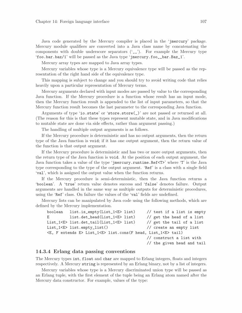
Chapter 14: Foreign language interface 107
Java code generated by the Mercury compiler is placed in the ‘jmercury’ package.Mercury module qualifiers are converted into a Java class name by concatenating thecomponents with double underscore separators (‘__’). For example the Mercury type‘foo.bar.baz/1’ will be passed as the Java type ‘jmercury.foo__bar.Baz_1’.
Mercury array types are mapped to Java array types.
Mercury variables whose type is a Mercury equivalence type will be passed as the rep-resentation of the right hand side of the equivalence type.
This mapping is subject to change and you should try to avoid writing code that reliesheavily upon a particular representation of Mercury terms.
Mercury arguments declared with input modes are passed by value to the correspondingJava function. If the Mercury procedure is a function whose result has an input mode,then the Mercury function result is appended to the list of input parameters, so that theMercury function result becomes the last parameter to the corresponding Java function.
Arguments of type ‘io.state’ or ‘store.store(_)’ are not passed or returned at all.(The reason for this is that these types represent mutable state, and in Java modificationsto mutable state are done via side effects, rather than argument passing.)
The handling of multiple output arguments is as follows.
If the Mercury procedure is deterministic and has no output arguments, then the returntype of the Java function is void; if it has one output argument, then the return value ofthe function is that output argument.
If the Mercury procedure is deterministic and has two or more output arguments, thenthe return type of the Java function is void. At the position of each output argument, theJava function takes a value of the type ‘jmercury.runtime.Ref<T>’ where ‘T’ is the Javatype corresponding to the type of the output argument. ‘Ref’ is a class with a single field‘val’, which is assigned the output value when the function returns.
If the Mercury procedure is semi-deterministic, then the Java function returns a‘boolean’. A ‘true’ return value denotes success and ‘false’ denotes failure. Outputarguments are handled in the same way as multiple outputs for deterministic procedures,using the ‘Ref’ class. On failure the values of the ‘val’ fields are undefined.
Mercury lists can be manipulated by Java code using the following methods, which aredefined by the Mercury implementation.
boolean list.is_empty(List_1<E> list) // test if a list is empty
E list.det_head(List_1<E> list) // get the head of a list
List_1<E> list.det_tail(List_1<E> list) // get the tail of a list
List_1<E> list.empty_list() // create an empty list
<E, F extends E> List_1<E> list.cons(F head, List_1<E> tail)
// construct a list with
// the given head and tail
14.3.4 Erlang data passing conventions
The Mercury types int, float and char are mapped to Erlang integers, floats and integersrespectively. A Mercury string is represented by an Erlang binary, not by a list of integers.
Mercury variables whose type is a Mercury discriminated union type will be passed asan Erlang tuple, with the first element of the tuple being an Erlang atom named after theMercury data constructor. For example, values of the type:

Chapter 14: Foreign language interface 108
:- type maybe_int
---> yes(int)
; no.
would be represented in Erlang as ‘{yes, integer}’ and ‘{no}’.
Mercury variables whose type is a Mercury equivalence type will be passed as the rep-resentation of the right hand side of the equivalence type.
This mapping is subject to change and you should try to avoid writing code that reliesheavily upon a particular representation of Mercury terms.
Arguments of dummy types, e.g. ‘io.state’, are represented by the atom ‘false’ whennecessary. They are not passed to and from calls to monomorphic procedures.
Mercury arguments declared with input modes are passed by value to the correspondingErlang function.
The result of an Erlang function depends on the determinism of the Mercury procedurethat it was derived from. Procedures which succeed exactly once and have a single outputvariable return the single value directly. Procedures which succeed exactly once and havezero or two or more output variables return a tuple of those output variables in order.
Procedures which are semideterministic return, on success, a tuple of the variables withoutput modes (including when the number of output variables is one). On failure theyreturn the Erlang atom ‘fail’.
Procedures which are nondeterministic take as a final argument a success continuation.This is an function which has an input variable for each variable of the Mercury procedurewith an output mode. For each solution, the success continuation is called with the valuesof those output variables. When there are no more solutions, the Erlang function returnswith an undefined value.
14.4 Using foreign types from Mercury
Types defined in a foreign language can be accessed in Mercury using a declaration of theform
:- pragma foreign_type(Lang, MercuryTypeName, ForeignTypeDescriptor).
This definesMercuryTypeName as a synonym for type ForeignTypeDescriptor defined inthe foreign language Lang. You must declareMercuryTypeName using a (possibly abstract)‘:- type’ declaration as usual. The ‘pragma foreign_type’ must not have wider visibilitythan the type declaration (if the ‘pragma foreign_type’ declaration is in the interface, the‘:- type’ declaration must be also).
ForeignTypeDescriptor defines how the Mercury type is mapped for a particular foreignlanguage. Specific syntax is given in the language specific information below.
MercuryTypeName is treated as an abstract type at all times in Mercury code. How-ever, if MercuryTypeName is one of the parameters of a foreign proc for Lang, and the‘pragma foreign_type’ declaration is visible to the foreign proc, it will be passed to thatforeign proc as specified by ForeignTypeDescriptor.
Multiple foreign language definitions may be given for the same type — the appropriatedefinition will be used for the appropriate language (see the language specific informationbelow for details). All definitions must have the same visibility. A Mercury definition, which

Chapter 14: Foreign language interface 109
must define a discriminated union type, may also be given. The constructors for the type willonly be visible in Mercury clauses for predicates or functions with ‘pragma foreign_proc’clauses for all of the languages for which there are ‘foreign_type’ declarations for the type.
You can also associate assertions about the properties of the foreign type with the‘foreign_type’ declaration, using the following syntax:
:- pragma foreign_type(Lang, MercuryTypeName, ForeignTypeDescriptor,
[ForeignTypeAssertion, ...]).
Currently, three kinds of assertions are supported.
The ‘can_pass_as_mercury_type’ assertion states that on the C backends, values ofthe given type can be passed to and from Mercury code without boxing, via simple casts,which is faster. This requires the type to be either an integer type or a pointer type, andrequires it to be castable to ‘MR_Word’ and back without loss of information (which meansthat its size may not be greater than the size of ‘MR_Word’).
The ‘word_aligned_pointer’ assertion implies ‘can_pass_as_mercury_type’ and ad-ditionally states that values of the given type are pointer values clear in the tag bits. Itallows the Mercury implementation to avoid boxing values of the given type when the typeappears as the sole argument of a data constructor.
The ‘stable’ assertion is meaningful only in the presence of the ‘can_pass_as_mercury_type’or ‘word_aligned_pointer’ assertions. It states that either the C type is an integertype, or it is a pointer type pointing to memory that will never change. Together, theseassertions are sufficient to allow tabling (see Section 19.2 [Tabled evaluation], page 145)and the ‘compare_representation’ primitive to work on values of such types.
Violations of any of these assertions are very likely to result in the generated executablesilently doing the wrong thing, giving no clue to where the problem might be. Since decidingwhether a C type satisfies the conditions of these assertions requires knowledge of theinternals of the Mercury implementation, we do not recommend the use of any of theseassertions unless you are confident of your expertise in those internals.
As with discriminated union types, programmers can specify the unification and/orcomparison predicates to use for values of the type using the following syntax (see Chapter 7[User-defined equality and comparison], page 56):
:- pragma foreign_type(Lang, MercuryTypeName, ForeignTypeDescriptor)
where equality is EqualityPred, comparison is ComparePred.
You can use Mercury foreign language interfacing declarations which specify languageX to interface to types that are actually written in a different language Y, provided thatX and Y have compatible interface conventions. Support for this kind of compatibility isdescribed in the language specific information below.
14.5 Using foreign enumerations in Mercury code
While a ‘pragma foreign_type’ declaration imports a foreign type into Mercury, a ‘pragmaforeign_enum’ declaration imports the values of the constants of an enumeration type intoMercury.
While languages such as C have special syntax for defining enumeration types, in Mer-cury, an enumeration type is simply an ordinary discriminated union type whose functionsymbols all have arity zero.

Chapter 14: Foreign language interface 110
Given an enumeration type such as
:- type unix_file_permissions
---> user_read
; user_write
; user_executable
; group_read
; group_write
; group_executable
; other_read
; other_write
; other_executable.
the values used to represent each constant are usually decided by the Mercury com-piler. However, the values assigned this way may not match the values expected by foreignlanguage code that uses values of the enumeration, and even if they happen to match,programmers probably would not want to rely on this coincidence.
This is why Mercury supports a mechanism that allows programmers to specify therepresentation of each constant in an enumeration type when generating code for a giventarget language. This mechanism is the ‘pragma foreign_enum’ declaration, which lookslike this:
:- pragma foreign_enum("C", unix_file_permissions/0,
[
user_read - "S_IRUSR",
user_write - "S_IWUSR",
user_executable - "S_IXUSR",
group_read - "S_IRGRP",
group_write - "S_IWGRP",
group_executable - "S_IXGRP",
other_read - "S_IROTH",
other_write - "S_IWOTH",
other_executable - "S_IXOTH"
]).
(Unix systems have a standard header file that defines each of ‘S_IRUSR’, . . . , ‘S_IXOTH’as macros that each expand to an integer constant; these constants happen not to be theones that the Mercury compiler would assign to those constants.)
The general form of ‘pragma foreign_enum’ declarations is
:- pragma foreign_enum("Lang", MercuryType, CtorValues).
where CtorValues is a list of pairs of the form:
[
ctor_0 - "ForeignValue_0",
ctor_1 - "ForeignValue_1",
...
ctor_N - "ForeignValue_N"
]
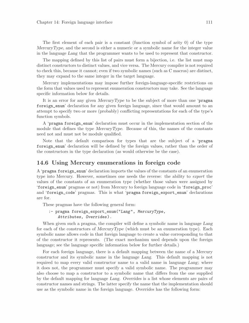
Chapter 14: Foreign language interface 111
The first element of each pair is a constant (function symbol of arity 0) of the typeMercuryType, and the second is either a numeric or a symbolic name for the integer valuein the language Lang that the programmer wants to be used to represent that constructor.
The mapping defined by this list of pairs must form a bijection, i.e. the list must mapdistinct constructors to distinct values, and vice versa. The Mercury compiler is not requiredto check this, because it cannot; even if two symbolic names (such as C macros) are distinct,they may expand to the same integer in the target language.
Mercury implementations may impose further foreign-language-specific restrictions onthe form that values used to represent enumeration constructors may take. See the languagespecific information below for details.
It is an error for any given MercuryType to be the subject of more than one ‘pragmaforeign_enum’ declaration for any given foreign language, since that would amount to anattempt to specify two or more (probably) conflicting representations for each of the type’sfunction symbols.
A ‘pragma foreign_enum’ declaration must occur in the implementation section of themodule that defines the type MercuryType. Because of this, the names of the constantsneed not and must not be module qualified.
Note that the default comparison for types that are the subject of a ‘pragmaforeign_enum’ declaration will be defined by the foreign values, rather than the order ofthe constructors in the type declaration (as would otherwise be the case).
14.6 Using Mercury enumerations in foreign code
A ‘pragma foreign_enum’ declaration imports the values of the constants of an enumerationtype into Mercury. However, sometimes one needs the reverse: the ability to export thevalues of the constants of an enumeration type (whether those values were assigned by‘foreign_enum’ pragmas or not) from Mercury to foreign language code in ‘foreign_proc’and ‘foreign_code’ pragmas. This is what ‘pragma foreign_export_enum’ declarationsare for.
These pragmas have the following general form:
:- pragma foreign_export_enum("Lang", MercuryType,
Attributes, Overrides).
When given such a pragma, the compiler will define a symbolic name in language Langfor each of the constructors of MercuryType (which must be an enumeration type). Eachsymbolic name allows code in that foreign language to create a value corresponding to thatof the constructor it represents. (The exact mechanism used depends upon the foreignlanguage; see the language specific information below for further details.)
For each foreign language, there is a default mapping between the name of a Mercuryconstructor and its symbolic name in the language Lang. This default mapping is notrequired to map every valid constructor name to a valid name in language Lang ; whereit does not, the programmer must specify a valid symbolic name. The programmer mayalso choose to map a constructor to a symbolic name that differs from the one suppliedby the default mapping for language Lang. Overrides is a list whose elements are pairs ofconstructor names and strings. The latter specify the name that the implementation shoulduse as the symbolic name in the foreign language. Overrides has the following form:
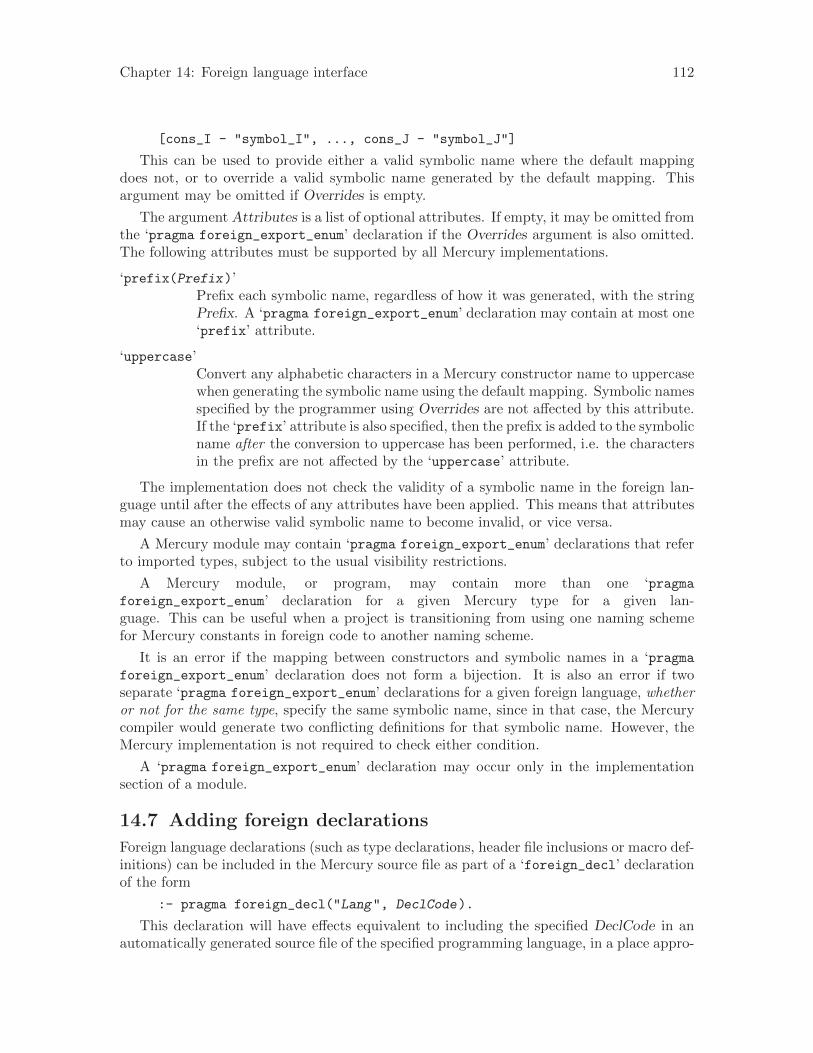
Chapter 14: Foreign language interface 112
[cons_I - "symbol_I", ..., cons_J - "symbol_J"]
This can be used to provide either a valid symbolic name where the default mappingdoes not, or to override a valid symbolic name generated by the default mapping. Thisargument may be omitted if Overrides is empty.
The argument Attributes is a list of optional attributes. If empty, it may be omitted fromthe ‘pragma foreign_export_enum’ declaration if the Overrides argument is also omitted.The following attributes must be supported by all Mercury implementations.
‘prefix(Prefix)’Prefix each symbolic name, regardless of how it was generated, with the stringPrefix. A ‘pragma foreign_export_enum’ declaration may contain at most one‘prefix’ attribute.
‘uppercase’Convert any alphabetic characters in a Mercury constructor name to uppercasewhen generating the symbolic name using the default mapping. Symbolic namesspecified by the programmer using Overrides are not affected by this attribute.If the ‘prefix’ attribute is also specified, then the prefix is added to the symbolicname after the conversion to uppercase has been performed, i.e. the charactersin the prefix are not affected by the ‘uppercase’ attribute.
The implementation does not check the validity of a symbolic name in the foreign lan-guage until after the effects of any attributes have been applied. This means that attributesmay cause an otherwise valid symbolic name to become invalid, or vice versa.
A Mercury module may contain ‘pragma foreign_export_enum’ declarations that referto imported types, subject to the usual visibility restrictions.
A Mercury module, or program, may contain more than one ‘pragmaforeign_export_enum’ declaration for a given Mercury type for a given lan-guage. This can be useful when a project is transitioning from using one naming schemefor Mercury constants in foreign code to another naming scheme.
It is an error if the mapping between constructors and symbolic names in a ‘pragmaforeign_export_enum’ declaration does not form a bijection. It is also an error if twoseparate ‘pragma foreign_export_enum’ declarations for a given foreign language, whetheror not for the same type, specify the same symbolic name, since in that case, the Mercurycompiler would generate two conflicting definitions for that symbolic name. However, theMercury implementation is not required to check either condition.
A ‘pragma foreign_export_enum’ declaration may occur only in the implementationsection of a module.
14.7 Adding foreign declarations
Foreign language declarations (such as type declarations, header file inclusions or macro def-initions) can be included in the Mercury source file as part of a ‘foreign_decl’ declarationof the form
:- pragma foreign_decl("Lang", DeclCode).
This declaration will have effects equivalent to including the specified DeclCode in anautomatically generated source file of the specified programming language, in a place appro-

Chapter 14: Foreign language interface 113
priate for declarations, and linking that source file with the Mercury program (after havingcompiled it with a compiler for the specified programming language, if appropriate).
Entities declared in ‘pragma foreign_decl’ declarations are visible in ‘pragmaforeign_code’, ‘pragma foreign_type’, ‘pragma foreign_proc’, and ‘pragmaforeign_enum’ declarations that specify the same foreign language and occur in the sameMercury module.
By default, the contents of ‘pragma foreign_decl’ declarations are also visible in thesame kinds of declarations in other modules that import the module containing the ‘pragmaforeign_decl’ declaration. This is because they may be required to make sense of types de-fined using ‘pragma foreign_type’ and/or predicates defined using ‘pragma foreign_proc’in the containing module, and these may be visible in other modules, especially in the pres-ence of intermodule optimization,
If you do not want the contents of a ‘pragma foreign_decl’ declaration to be visible inforeign language code in other modules, you can use the following variant of the declaration:
:- pragma foreign_decl("Lang", local, DeclCode).
Note: currently only the C and Erlang backends support this variant of the ‘pragmaforeign_decl’ declaration.
The Melbourne Mercury implementation additionally supports the forms
:- pragma foreign_decl("Lang", include_file("Path")).
:- pragma foreign_decl("Lang", local, include_file("Path")).
These have the same effects as the standard forms except that the contents of the filereferenced by Path are included in place of the string literal in the last argument, withoutfurther interpretation. Path may be an absolute path to a file, or a path to a file relativeto the directory that contains the source file of the module containing the declaration. Theinterpretation of the path is platform-dependent. If the filesystem uses a different characterset or encoding from the Mercury source file (which must be UTF-8), the file may not befound.
‘mmc --make’ and ‘mmake’ treat included files as dependencies of the module.
14.8 Declaring Mercury exports to other modules
The declarations for Mercury predicates or functions exported to a foreign languageusing a ‘pragma foreign_export’ declaration are visible to foreign code in a ‘pragmaforeign_code’ or ‘pragma foreign_proc’ declaration of the same module, and also inthose of any submodules. By default, they are not visible to the foreign code in ‘pragmaforeign_code’ or ‘pragma foreign_proc’ declarations in any other module, but thisdefault can be overridden (giving access to all other modules) using a declaration of theform:
:- pragma foreign_import_module("Lang", ImportedModule).
where ImportedModule is the name of the module containing the ‘pragma foreign_export’declarations.
If Lang is "C", this is equivalent to
:- pragma foreign_decl("C", "#include ""ImportedModule.mh""").
where ‘ImportedModule.mh’ is the automatically generated header file containing the Cdeclarations for the predicates and functions exported to C.

Chapter 14: Foreign language interface 114
‘pragma foreign_import_module’ should be used instead of the explicit#include because ‘pragma foreign_import_module’ tells the implementation that‘ImportedModule.mh’ must be built before the object file for the module containing the‘pragma foreign_import_module’ declaration.
Note that the Melbourne Mercury implementation often behaves as if ‘pragmaforeign_import_module’ declarations were implicitly added to modules. However,programmers should not should not depend on this behaviour; they should always writeexplicit ‘pragma foreign_import_module’ declarations wherever they are needed.
14.9 Adding foreign definitions
Definitions of foreign language entities (such as functions or global variables) may be in-cluded using a declaration of the form
:- pragma foreign_code("Lang", Code).
This declaration will have effects equivalent to including the specified Code in an auto-matically generated source file of the specified programming language, in a place appropriatefor definitions, and linking that source file with the Mercury program (after having compiledit with a compiler for the specified programming language, if appropriate).
Entities declared in ‘pragma foreign_code’ declarations are visible in ‘pragmaforeign_proc’ declarations that specify the same foreign language and occur in the sameMercury module.
The Melbourne Mercury implementation additionally supports the form
:- pragma foreign_code("Lang", include_file("Path")).
This has the same effect as the standard form except that the contents of the file ref-erenced by Path are included in place of the string literal in the last argument, withoutfurther interpretation. Path may be an absolute path to a file, or a path to a file relativeto the directory that contains the source file of the module containing the declaration. Theinterpretation of the path is platform-dependent. If the filesystem uses a different characterset or encoding from the Mercury source file (which must be UTF-8), the file may not befound.
‘mmc --make’ and ‘mmake’ treat included files as dependencies of the module.
14.10 Language specific bindings
All Mercury implementations should support interfacing with C. The set of other languagessupported is implementation-defined. A suitable compiler or assembler for the foreign lan-guage must be available on the system.
The Melbourne Mercury implementation supports interfacing with the following lan-guages:
‘C’ Use the string "C" to set the foreign language to C.
‘C#’ Use the string "C#" to set the foreign language to C#.
‘Java’ Use the string "Java" to set the foreign language to Java.
‘Erlang’ Use the string "Erlang" to set the foreign language to Erlang.
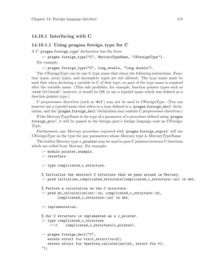
Chapter 14: Foreign language interface 115
14.10.1 Interfacing with C
14.10.1.1 Using pragma foreign type for C
A C ‘pragma foreign_type’ declaration has the form:
:- pragma foreign_type("C", MercuryTypeName, "CForeignType").
For example,
:- pragma foreign_type("C", long_double, "long double").
The CForeignType can be any C type name that obeys the following restrictions. Func-tion types, array types, and incomplete types are not allowed. The type name must besuch that when declaring a variable in C of that type, no part of the type name is requiredafter the variable name. (This rule prohibits, for example, function pointer types such as‘void (*)(void)’; however, it would be OK to use a typedef name which was defined as afunction pointer type.)
C preprocessor directives (such as ‘#if’) may not be used in CForeignType. (You canhowever use a typedef name that refers to a type defined in a ‘pragma foreign_decl’ decla-ration, and the ‘pragma foreign_decl’ declaration may contain C preprocessor directives.)
If theMercuryTypeName is the type of a parameter of a procedure defined using ‘pragmaforeign_proc’, it will be passed to the foreign proc’s foreign language code as CForeign-Type.
Furthermore, any Mercury procedure exported with ‘pragma foreign_export’ will useCForeignType as the type for any parameters whose Mercury type is MercuryTypeName.
The builtin Mercury type c_pointermay be used to pass C pointers between C functionswhich are called from Mercury. For example:
:- module pointer_example.
:- interface.
:- type complicated_c_structure.
% Initialise the abstract C structure that we pass around in Mercury.
:- pred initialise_complicated_structure(complicated_c_structure::uo) is det.
% Perform a calculation on the C structure.
:- pred do_calculation(int::in, complicated_c_structure::di,
complicated_c_structure::uo) is det.
:- implementation.
% Our C structure is implemented as a c_pointer.
:- type complicated_c_structure
---> complicated_c_structure(c_pointer).
:- pragma foreign_decl("C",
extern struct foo *init_struct(void);
extern struct foo *perform_calculation(int, struct foo *);
");

Chapter 14: Foreign language interface 116
:- pragma foreign_proc("C",
initialise_complicated_structure(Structure::uo),
[will_not_call_mercury, may_call_mercury],
"
Structure = init_struct();
").
:- pragma foreign_proc("C",
do_calculation(Value::in, Structure0::di, Structure::uo),
[will_not_call_mercury, may_call_mercury],
"
Structure = perform_calculation(Value, Structure0);
").
We strongly recommend the use of ‘pragma foreign_type’ instead of c_pointer as theuse of ‘pragma foreign_type’ results in more type-safe code.
14.10.1.2 Using pragma foreign enum for C
Foreign enumeration values in C must be constants of type MR_Integer. They may bespecified as either integer literals or via preprocessor macros that expand to integer literals.
14.10.1.3 Using pragma foreign export enum for C
For C the symbolic names generated by a ‘pragma foreign_export_enum’ must formvalid C identifiers. These identifiers are used as the names of preprocessor macros.The body of each of these macros expands to a value that is identical to that of theconstructor to which the symbolic name corresponds in the mapping established by the‘pragma foreign_export_enum’ declaration.
As noted in the Section 14.3.1 [C data passing conventions], page 102, the type of thesevalues is MR_Word.
The default mapping used by ‘pragma foreign_export_enum’ declarations for C is touse the Mercury constructor name as the base of the symbolic name. For example, thesymbolic name for the Mercury constructor ‘foo’ would be foo.
14.10.1.4 Using pragma foreign proc for C
The input and output variables will have C types corresponding to their Mercury types, asdetermined by the rules specified in Section 14.3.1 [C data passing conventions], page 102.
The C code fragment may declare local variables, up to a total size of 10kB for theprocedure. If a procedure requires more than this for its local variables, the code canbe moved into a separate function (defined in a ‘pragma foreign_code’ declaration, forexample).
The C code fragment should not declare any labels or static variables unless there is alsoa ‘pragma no_inline’ declaration or a ‘may_not_duplicate’ foreign code attribute for theprocedure. The reason for this is that otherwise the Mercury implementation may inlinethe procedure by duplicating the C code fragment for each call. If the C code fragmentdeclared a static variable, inlining it in this way could result in the program having multiple

Chapter 14: Foreign language interface 117
instances of the static variable, rather than a single shared instance. If the C code fragmentdeclared a label, inlining it in this way could result in an error due to the same label beingdefined twice inside a single C function.
C code in a pragma foreign_proc declaration for any procedure whose determinismindicates that it can fail must assign a truth value to the macro SUCCESS_INDICATOR. Forexample:
:- pred string.contains_char(string, character).
:- mode string.contains_char(in, in) is semidet.
:- pragma foreign_proc("C",
string.contains_char(Str::in, Ch::in),
[will_not_call_mercury, promise_pure],
"
SUCCESS_INDICATOR = (strchr(Str, Ch) != NULL);
").
SUCCESS_INDICATOR should not be used other than as the target of an assignment. (Forexample, it may be #defined to a register, so you should not try to take its address.)Procedures whose determinism indicates that they cannot fail should not access SUCCESS_INDICATOR.
Arguments whose mode is input will have their values set by the Mercury implementationon entry to the C code. If the procedure succeeds, the C code must set the values of alloutput arguments. If the procedure fails, the C code need only set SUCCESS_INDICATOR tofalse (zero).
The behaviour of a procedure defined using a ‘pragma foreign_proc’ declaration whosebody contains a return statement is undefined.
14.10.1.5 Using pragma foreign export for C
A ‘pragma foreign_export’ declaration for C has the form:
:- pragma foreign_export("C", MercuryMode, "C_Name").
For example,
:- pragma foreign_export("C", foo(in, in, out), "FOO").
For each Mercury module containing ‘pragma foreign_export’ declarations for C, theMercury implementation will automatically create a header file for that module which de-clares a C function C Name() for each of the ‘pragma foreign_export’ declarations. Eachsuch C function is the C interface to the specified Mercury procedure.
The type signature of the C interface to a Mercury procedure is determined as follows.Mercury types are converted to C types according to the rules in Section 14.3.1 [C datapassing conventions], page 102. Input arguments are passed by value. For output arguments,the caller must pass the address in which to store the result. If the Mercury procedure canfail, then its C interface function returns a truth value indicating success or failure. Ifthe Mercury procedure is a Mercury function that cannot fail, and the function result hasan output mode, then the C interface function will return the Mercury function resultvalue. Otherwise the function result is appended as an extra argument. Arguments of type‘io.state’ or ‘store.store(_)’ are not passed at all. (The reason for this is that these

Chapter 14: Foreign language interface 118
types represent mutable state, and in C modifications to mutable state are done via sideeffects, rather than argument passing.)
Calling polymorphically typed Mercury procedures from C is a little bit more difficultthan calling ordinary (monomorphically typed) Mercury procedures. The simplest methodis to just create monomorphic forwarding procedures that call the polymorphic procedures,and export them, rather than exporting the polymorphic procedures.
If you do export a polymorphically typed Mercury procedure, the compiler will prependone ‘type_info’ argument to the parameter list of the C interface function for each distincttype variable in the Mercury procedure’s type signature. The caller must arrange to pass inappropriate ‘type_info’ values corresponding to the types of the other arguments passed.These ‘type_info’ arguments can be obtained using the Mercury ‘type_of’ function in theMercury standard library module ‘type_desc’.
To use the C declarations produced see Section 14.10.1.6 [Using pragma foreign decl forC], page 118.
Throwing an exception across the C interface is not supported. That is, if a Mercuryprocedure that is exported to C using ‘pragma foreign_export’ throws an exception whichis not caught within that procedure, then you will get undefined behaviour.
14.10.1.6 Using pragma foreign decl for C
Any macros, function prototypes, or other C declarations that are used in ‘foreign_code’,‘foreign_type’ or ‘foreign_proc’ pragmas must be included using a ‘foreign_decl’ dec-laration of the form
:- pragma foreign_decl("C", HeaderCode).
HeaderCode can be a C ‘#include’ line, for example
:- pragma foreign_decl("C", "#include <math.h>")
or
:- pragma foreign_decl("C", "#include ""tcl.h""").
or it may contain any C declarations, for example
:- pragma foreign_decl("C", "
extern int errno;
#define SIZE 200
struct Employee {
char name[SIZE];
};
extern int bar;
extern void foo(void);
").
Mercury automatically includes certain headers such as <stdlib.h>, but you shouldnot rely on this, as the set of headers which Mercury automatically includes is subject tochange.
If a Mercury predicate or function exported using a ‘pragma foreign_export’ declara-tion is to be used within a ‘:- pragma foreign_code’ or ‘:- pragma foreign_proc’ decla-ration the header file for the module containing the ‘pragma foreign_export’ declarationshould be included using a ‘pragma foreign_import_module’ declaration, for example
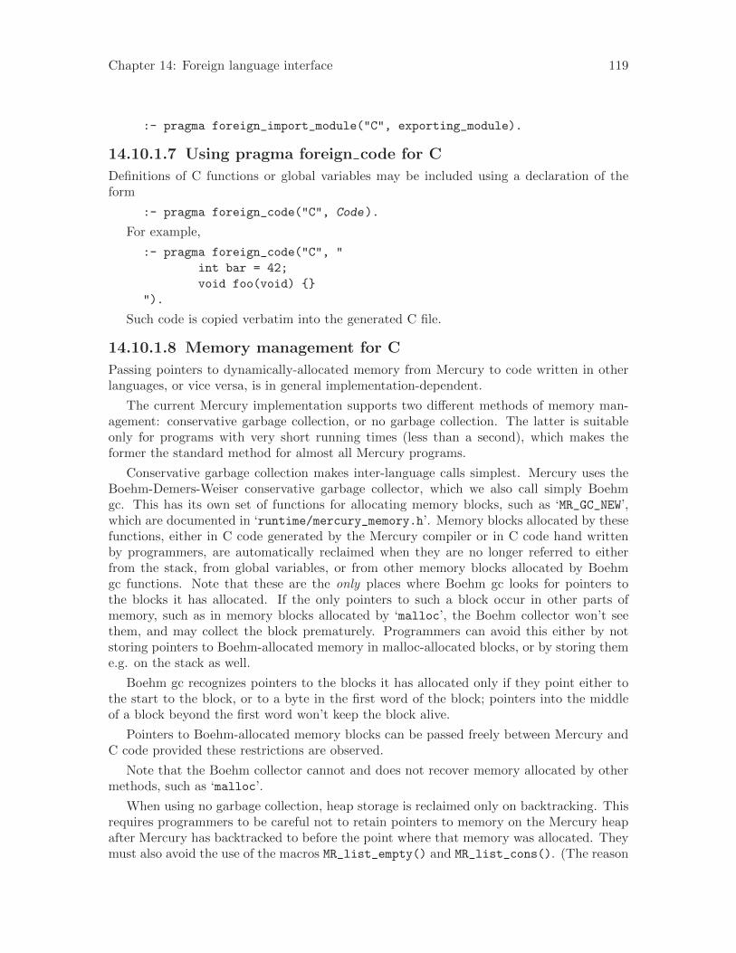
Chapter 14: Foreign language interface 119
:- pragma foreign_import_module("C", exporting_module).
14.10.1.7 Using pragma foreign code for C
Definitions of C functions or global variables may be included using a declaration of theform
:- pragma foreign_code("C", Code).
For example,
:- pragma foreign_code("C", "
int bar = 42;
void foo(void) {}
").
Such code is copied verbatim into the generated C file.
14.10.1.8 Memory management for C
Passing pointers to dynamically-allocated memory from Mercury to code written in otherlanguages, or vice versa, is in general implementation-dependent.
The current Mercury implementation supports two different methods of memory man-agement: conservative garbage collection, or no garbage collection. The latter is suitableonly for programs with very short running times (less than a second), which makes theformer the standard method for almost all Mercury programs.
Conservative garbage collection makes inter-language calls simplest. Mercury uses theBoehm-Demers-Weiser conservative garbage collector, which we also call simply Boehmgc. This has its own set of functions for allocating memory blocks, such as ‘MR_GC_NEW’,which are documented in ‘runtime/mercury_memory.h’. Memory blocks allocated by thesefunctions, either in C code generated by the Mercury compiler or in C code hand writtenby programmers, are automatically reclaimed when they are no longer referred to eitherfrom the stack, from global variables, or from other memory blocks allocated by Boehmgc functions. Note that these are the only places where Boehm gc looks for pointers tothe blocks it has allocated. If the only pointers to such a block occur in other parts ofmemory, such as in memory blocks allocated by ‘malloc’, the Boehm collector won’t seethem, and may collect the block prematurely. Programmers can avoid this either by notstoring pointers to Boehm-allocated memory in malloc-allocated blocks, or by storing theme.g. on the stack as well.
Boehm gc recognizes pointers to the blocks it has allocated only if they point either tothe start to the block, or to a byte in the first word of the block; pointers into the middleof a block beyond the first word won’t keep the block alive.
Pointers to Boehm-allocated memory blocks can be passed freely between Mercury andC code provided these restrictions are observed.
Note that the Boehm collector cannot and does not recover memory allocated by othermethods, such as ‘malloc’.
When using no garbage collection, heap storage is reclaimed only on backtracking. Thisrequires programmers to be careful not to retain pointers to memory on the Mercury heapafter Mercury has backtracked to before the point where that memory was allocated. Theymust also avoid the use of the macros MR_list_empty() and MR_list_cons(). (The reason

Chapter 14: Foreign language interface 120
for this is that they may access Mercury’s ‘MR_hp’ register, which might not be valid in Ccode. Using them in the bodies of procedures defined using ‘pragma foreign_proc’ with‘will_not_call_mercury’ would probably work, but we don’t advise it.) Instead, you canwrite Mercury functions to perform these actions and use ‘pragma foreign_export’ to ac-cess them from C. This alternative method also works with conservative garbage collection.
Future Mercury implementations may use non-conservative methods of garbage collec-tion. For such implementations, it will be necessary to explicitly register pointers passedto C with the garbage collector. The mechanism for doing this has not yet been decidedon. It would be desirable to provide a single memory management interface for use wheninterfacing with other languages that can work for all methods of memory management,but more implementation experience is needed before we can formulate such an interface.
14.10.1.9 Linking with C object files
A Mercury implementation should allow you to link with object files or libraries that wereproduced by compiling C code. The exact mechanism for linking with C object files isimplementation-dependent. The following text describes how it is done for the MelbourneMercury implementation.
To link an existing object file or archive of object files into your Mercury code, use thecommand line option ‘--link-object’. For example, the following will link the object file‘my_function.o’ from the current directory when compiling the program ‘prog’:
mmc --link-object my_functions.o prog
The command line option ‘--library’ (or ‘-l’ for short) can be used to link an exist-ing library into your Mercury code. For example, the following will link the library file‘libfancy_library.a’, or perhaps the shared version ‘libfancy_library.so’, from thedirectory ‘/usr/local/contrib/lib’, when compiling the program ‘prog’:
mmc -R/usr/local/contrib/lib -L/usr/local/contrib/lib -lfancy_library prog
As illustrated by the example, the command line options ‘-R’, ‘-L’ and ‘-l’, have thesame meaning as they do with the Unix linker.
For more information, see the “Libraries” chapter of the Mercury User’s Guide.
14.10.2 Interfacing with C#
14.10.2.1 Using pragma foreign type for C#
A C# ‘pragma foreign_type’ declaration has the form:
:- pragma foreign_type("C#", MercuryTypeName, "C#-Type").
The C#-Type can be any accessible C# type.
The effect of this declaration is that Mercury values of type MercuryTypeName will bepassed to and from C# foreign procs as having type C#-Type.
Furthermore, any Mercury procedure exported with ‘pragma foreign_export’ will useC#-Type as the type for any parameters whose Mercury type is MercuryTypeName.
14.10.2.2 Using pragma foreign enum for C#
Foreign enumeration values in C# must be a constant value expression which is a validinitializer within an enumeration of underlying type int.

Chapter 14: Foreign language interface 121
14.10.2.3 Using pragma foreign export enum for C#
For C# the symbolic names generated by a ‘pragma foreign_export_enum’ must formvalid C# identifiers. These identifiers are used as the names of static class members.
The default mapping used by ‘pragma foreign_export_enum’ declarations for C# is touse the Mercury constructor name as the base of the symbolic name. For example, thesymbolic name for the Mercury constructor ‘foo’ would be foo.
14.10.2.4 Using pragma foreign proc for C#
The C# code from C# ‘pragma foreign_proc’ declarations will be placed in the bodies ofstatic member functions of an automatically generated C# class. Since such C# code willbecome part of a static member function, it must not refer to the this keyword. It mayhowever refer to static member variables or static member functions declared with ‘pragmaforeign_code’.
The input and output variables for a C# ‘pragma foreign_proc’ will have C# typescorresponding to their Mercury types. The exact rules for mapping Mercury types to C#types are described in Section 14.3.2 [C# data passing conventions], page 103.
C# code in a pragma foreign_proc declaration for any procedure whose determinism in-dicates that it can fail must assign a value of type bool to the variable SUCCESS_INDICATOR.For example:
:- pred string.contains_char(string, character).
:- mode string.contains_char(in, in) is semidet.
:- pragma foreign_proc("C#",
string.contains_char(Str::in, Ch::in),
[will_not_call_mercury, promise_pure],
"
SUCCESS_INDICATOR = (Str.IndexOf(Ch) != -1);
").
C# code for procedures whose determinism indicates that they cannot fail should not accessSUCCESS_INDICATOR.
Arguments whose mode is input will have their values set by the Mercury implementationon entry to the C# code. If the procedure succeeds, the C# code must set the values of alloutput arguments. If the procedure fails, the C# code need only set SUCCESS_INDICATORto false.
14.10.2.5 Using pragma foreign export for C#
A ‘pragma foreign_export’ declaration for C# has the form:
:- pragma foreign_export("C#", MercuryMode, "C#_Name").
For example,
:- pragma foreign_export("C#", foo(in, in, out), "FOO").
The type signature of the C# interface to a Mercury procedure is as described inSection 14.3.2 [C# data passing conventions], page 103.
Calling polymorphically typed Mercury procedures from C# is a little bit more difficultthan calling ordinary (monomorphically typed) Mercury procedures. The simplest method
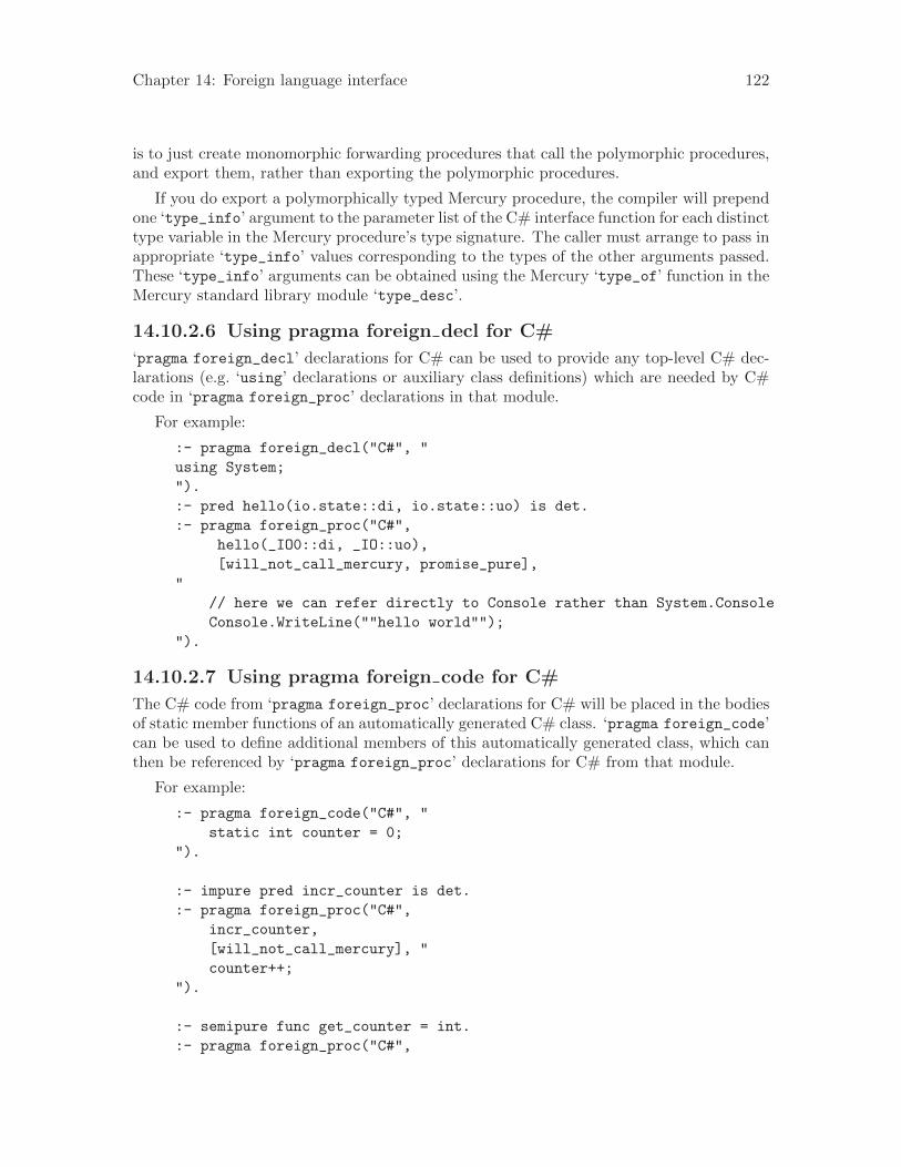
Chapter 14: Foreign language interface 122
is to just create monomorphic forwarding procedures that call the polymorphic procedures,and export them, rather than exporting the polymorphic procedures.
If you do export a polymorphically typed Mercury procedure, the compiler will prependone ‘type_info’ argument to the parameter list of the C# interface function for each distincttype variable in the Mercury procedure’s type signature. The caller must arrange to pass inappropriate ‘type_info’ values corresponding to the types of the other arguments passed.These ‘type_info’ arguments can be obtained using the Mercury ‘type_of’ function in theMercury standard library module ‘type_desc’.
14.10.2.6 Using pragma foreign decl for C#
‘pragma foreign_decl’ declarations for C# can be used to provide any top-level C# dec-larations (e.g. ‘using’ declarations or auxiliary class definitions) which are needed by C#code in ‘pragma foreign_proc’ declarations in that module.
For example:
:- pragma foreign_decl("C#", "
using System;
").
:- pred hello(io.state::di, io.state::uo) is det.
:- pragma foreign_proc("C#",
hello(_IO0::di, _IO::uo),
[will_not_call_mercury, promise_pure],
"
// here we can refer directly to Console rather than System.Console
Console.WriteLine(""hello world"");
").
14.10.2.7 Using pragma foreign code for C#
The C# code from ‘pragma foreign_proc’ declarations for C# will be placed in the bodiesof static member functions of an automatically generated C# class. ‘pragma foreign_code’can be used to define additional members of this automatically generated class, which canthen be referenced by ‘pragma foreign_proc’ declarations for C# from that module.
For example:
:- pragma foreign_code("C#", "
static int counter = 0;
").
:- impure pred incr_counter is det.
:- pragma foreign_proc("C#",
incr_counter,
[will_not_call_mercury], "
counter++;
").
:- semipure func get_counter = int.
:- pragma foreign_proc("C#",
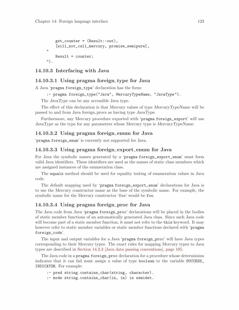
Chapter 14: Foreign language interface 123
get_counter = (Result::out),
[will_not_call_mercury, promise_semipure],
"
Result = counter;
").
14.10.3 Interfacing with Java
14.10.3.1 Using pragma foreign type for Java
A Java ‘pragma foreign_type’ declaration has the form:
:- pragma foreign_type("Java", MercuryTypeName, "JavaType").
The JavaType can be any accessible Java type.
The effect of this declaration is that Mercury values of type MercuryTypeName will bepassed to and from Java foreign procs as having type JavaType.
Furthermore, any Mercury procedure exported with ‘pragma foreign_export’ will useJavaType as the type for any parameters whose Mercury type is MercuryTypeName.
14.10.3.2 Using pragma foreign enum for Java
‘pragma foreign_enum’ is currently not supported for Java.
14.10.3.3 Using pragma foreign export enum for Java
For Java the symbolic names generated by a ‘pragma foreign_export_enum’ must formvalid Java identifiers. These identifiers are used as the names of static class members whichare assigned instances of the enumeration class.
The equals method should be used for equality testing of enumeration values in Javacode.
The default mapping used by ‘pragma foreign_export_enum’ declarations for Java isto use the Mercury constructor name as the base of the symbolic name. For example, thesymbolic name for the Mercury constructor ‘foo’ would be foo.
14.10.3.4 Using pragma foreign proc for Java
The Java code from Java ‘pragma foreign_proc’ declarations will be placed in the bodiesof static member functions of an automatically generated Java class. Since such Java codewill become part of a static member function, it must not refer to the this keyword. It mayhowever refer to static member variables or static member functions declared with ‘pragmaforeign_code’.
The input and output variables for a Java ‘pragma foreign_proc’ will have Java typescorresponding to their Mercury types. The exact rules for mapping Mercury types to Javatypes are described in Section 14.3.3 [Java data passing conventions], page 105.
The Java code in a pragma foreign_proc declaration for a procedure whose determinismindicates that it can fail must assign a value of type boolean to the variable SUCCESS_
INDICATOR. For example:
:- pred string.contains_char(string, character).
:- mode string.contains_char(in, in) is semidet.
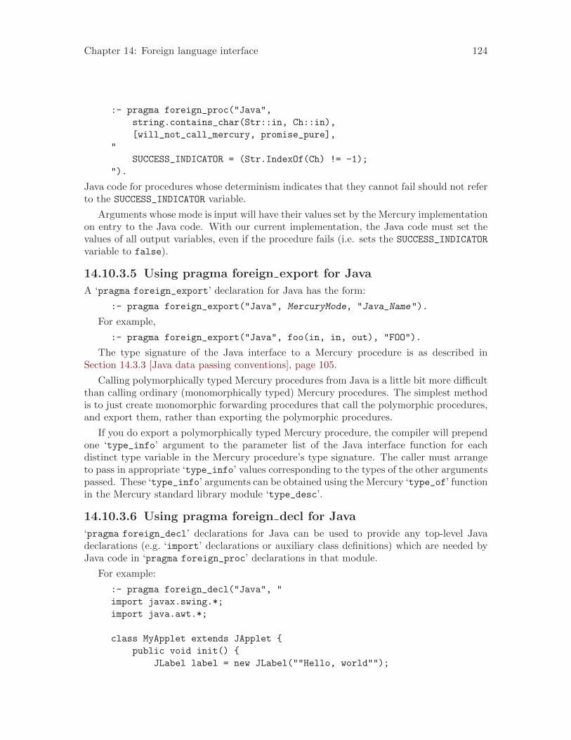
Chapter 14: Foreign language interface 124
:- pragma foreign_proc("Java",
string.contains_char(Str::in, Ch::in),
[will_not_call_mercury, promise_pure],
"
SUCCESS_INDICATOR = (Str.IndexOf(Ch) != -1);
").
Java code for procedures whose determinism indicates that they cannot fail should not referto the SUCCESS_INDICATOR variable.
Arguments whose mode is input will have their values set by the Mercury implementationon entry to the Java code. With our current implementation, the Java code must set thevalues of all output variables, even if the procedure fails (i.e. sets the SUCCESS_INDICATORvariable to false).
14.10.3.5 Using pragma foreign export for Java
A ‘pragma foreign_export’ declaration for Java has the form:
:- pragma foreign_export("Java", MercuryMode, "Java_Name").
For example,
:- pragma foreign_export("Java", foo(in, in, out), "FOO").
The type signature of the Java interface to a Mercury procedure is as described inSection 14.3.3 [Java data passing conventions], page 105.
Calling polymorphically typed Mercury procedures from Java is a little bit more difficultthan calling ordinary (monomorphically typed) Mercury procedures. The simplest methodis to just create monomorphic forwarding procedures that call the polymorphic procedures,and export them, rather than exporting the polymorphic procedures.
If you do export a polymorphically typed Mercury procedure, the compiler will prependone ‘type_info’ argument to the parameter list of the Java interface function for eachdistinct type variable in the Mercury procedure’s type signature. The caller must arrangeto pass in appropriate ‘type_info’ values corresponding to the types of the other argumentspassed. These ‘type_info’ arguments can be obtained using the Mercury ‘type_of’ functionin the Mercury standard library module ‘type_desc’.
14.10.3.6 Using pragma foreign decl for Java
‘pragma foreign_decl’ declarations for Java can be used to provide any top-level Javadeclarations (e.g. ‘import’ declarations or auxiliary class definitions) which are needed byJava code in ‘pragma foreign_proc’ declarations in that module.
For example:
:- pragma foreign_decl("Java", "
import javax.swing.*;
import java.awt.*;
class MyApplet extends JApplet {
public void init() {
JLabel label = new JLabel(""Hello, world"");

Chapter 14: Foreign language interface 125
label.setHorizontalAlignment(JLabel.CENTER);
getContentPane().add(label);
}
}
").
:- pred hello(io.state::di, io.state::uo) is det.
:- pragma foreign_proc("Java",
hello(_IO0::di, _IO::uo),
[will_not_call_mercury],
"
MyApplet app = new MyApplet();
// ...
").
14.10.3.7 Using pragma foreign code for Java
The Java code from ‘pragma foreign_proc’ declarations for Java will be placed in thebodies of static member functions of an automatically generated Java class. ‘pragmaforeign_code’ can be used to define additional members of this automatically generatedclass, which can then be referenced by ‘pragma foreign_proc’ declarations for Java fromthat module.
For example:
:- pragma foreign_code("Java", "
static int counter = 0;
").
:- impure pred incr_counter is det.
:- pragma foreign_proc("Java",
incr_counter,
[will_not_call_mercury],
"
counter++;
").
:- semipure func get_counter = int.
:- pragma foreign_proc("Java",
get_counter = (Result::out),
[will_not_call_mercury, promise_semipure],
"
Result = counter;
").
14.10.4 Interfacing with Erlang
14.10.4.1 Using pragma foreign type for Erlang
An Erlang ‘pragma foreign_type’ declaration has the form:
:- pragma foreign_type("Erlang", MercuryTypeName, "").

Chapter 14: Foreign language interface 126
The effect of this declaration is that Mercury values of type MercuryTypeName willbe passed to and from Erlang foreign procs as having some representation unknown toMercury.
14.10.4.2 Using pragma foreign export enum for Erlang
Values of Mercury enumeration types may be referred to from Erlang code using the conven-tion for discriminated union types described in Section 14.3.4 [Erlang data passing conven-tions], page 107. As such, ‘pragma foreign_export_enum’ declarations are neither requiredor supported for Erlang.
14.10.4.3 Using pragma foreign proc for Erlang
The input and output variables for a Erlang ‘pragma foreign_proc’ will be the Erlangrepresentations as described in Section 14.3.4 [Erlang data passing conventions], page 107.
The Erlang code in a pragma foreign_proc declaration for a procedure whose determin-ism indicates that it can fail must assign either ‘true’ or ‘false’ to the variable SUCCESS_INDICATOR. For example:
:- pred contains_char(list(char)::in, char::in) is semidet.
:- pragma foreign_proc("Erlang",
contains_char(Str::in, Ch::in),
[will_not_call_mercury, promise_pure, thread_safe],
"
SUCCESS_INDICATOR = (string:chr(Str, Ch) =/= 0)
").
Arguments whose mode is input will have their values set by the Mercury implementationon entry to the Erlang code. The Erlang code must set the values of all output variables,even if the procedure fails (i.e. sets the SUCCESS_INDICATOR variable to false).
14.10.4.4 Using pragma foreign export for Erlang
A ‘pragma foreign_export’ declaration for Erlang has the form:
:- pragma foreign_export("Erlang", MercuryMode, "Erlang_Name").
For example,
:- pragma foreign_export("Erlang", foo(in, in, out), "foo").
The type signature of the Erlang interface to a Mercury procedure is described inSection 14.3.4 [Erlang data passing conventions], page 107.
Calling polymorphically typed Mercury procedures from Erlang is a little bit more dif-ficult than calling ordinary (monomorphically typed) Mercury procedures. The simplestmethod is to just create monomorphic forwarding procedures that call the polymorphicprocedures, and export them, rather than exporting the polymorphic procedures.
If you do export a polymorphically typed Mercury procedure, the compiler will prependone ‘type_info’ argument to the parameter list of the Erlang interface function for eachdistinct type variable in the Mercury procedure’s type signature. The caller must arrange topass in appropriate ‘type_info’ values corresponding to the types of the other argumentspassed. These ‘type_info’ arguments can be obtained using the Mercury ‘type_of’ functionin the Mercury standard library module ‘type_desc’.
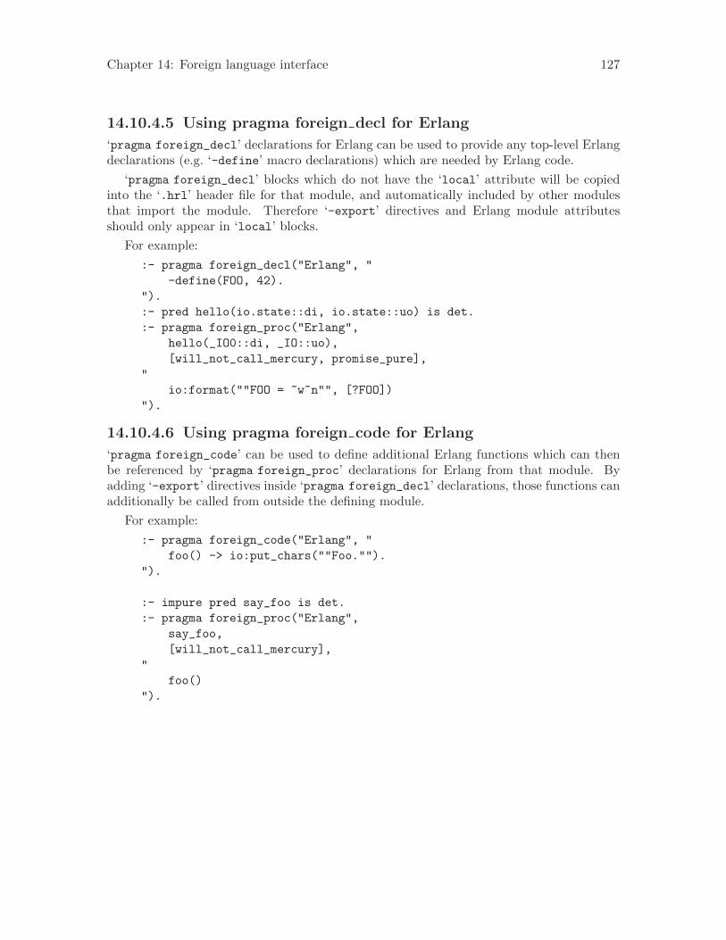
Chapter 14: Foreign language interface 127
14.10.4.5 Using pragma foreign decl for Erlang
‘pragma foreign_decl’ declarations for Erlang can be used to provide any top-level Erlangdeclarations (e.g. ‘-define’ macro declarations) which are needed by Erlang code.
‘pragma foreign_decl’ blocks which do not have the ‘local’ attribute will be copiedinto the ‘.hrl’ header file for that module, and automatically included by other modulesthat import the module. Therefore ‘-export’ directives and Erlang module attributesshould only appear in ‘local’ blocks.
For example:
:- pragma foreign_decl("Erlang", "
-define(FOO, 42).
").
:- pred hello(io.state::di, io.state::uo) is det.
:- pragma foreign_proc("Erlang",
hello(_IO0::di, _IO::uo),
[will_not_call_mercury, promise_pure],
"
io:format(""FOO = ~w~n"", [?FOO])
").
14.10.4.6 Using pragma foreign code for Erlang
‘pragma foreign_code’ can be used to define additional Erlang functions which can thenbe referenced by ‘pragma foreign_proc’ declarations for Erlang from that module. Byadding ‘-export’ directives inside ‘pragma foreign_decl’ declarations, those functions canadditionally be called from outside the defining module.
For example:
:- pragma foreign_code("Erlang", "
foo() -> io:put_chars(""Foo."").
").
:- impure pred say_foo is det.
:- pragma foreign_proc("Erlang",
say_foo,
[will_not_call_mercury],
"
foo()
").
Chapter 15: Impurity declarations 128
15 Impurity declarations
In order to efficiently implement certain predicates, it is occasionally necessary to ventureoutside pure logic programming. Other predicates cannot be implemented at all within theparadigm of logic programming, for example, all solutions predicates. Such predicates areoften written using the foreign language interface. Sometimes, however, it would be moreconvenient, or more efficient, to write such predicates using the facilities of Mercury. Forexample, it is much more convenient to access arguments of compound Mercury terms inMercury than in C, and the ability of the Mercury compiler to specialize code can makehigher-order predicates written in Mercury significantly more efficient than similar C code.
One important aim of Mercury’s impurity system is to make the distinction betweenthe pure and impure code very clear. This is done by requiring every impure predicate orfunction to be so declared, and by requiring every call to an impure predicate or functionto be flagged as such. Predicates or functions that are implemented in terms of impurepredicates or functions are assumed to be impure themselves unless they are explicitlypromised to be pure.
Please note that the facilities described here are needed only very rarely. The mainintent is for implementing language primitives such as the all solutions predicates, or forimplementing interfaces to foreign language libraries using the foreign language interface.Any other use of ‘impure’ or ‘semipure’ probably indicates either a weakness in the Mer-cury standard library, or the programmer’s lack of familiarity with the standard library.Newcomers to Mercury are hence encouraged to skip this section.
15.1 Choosing the right level of purity
Mercury distinguishes three “levels” of purity:
pure For pure procedures, the set of solutions depends only on the values of theinput arguments. They do not interact with the “real” world (i.e., do anyinput/output) without taking an io.state (see Chapter 3 [Types], page 27) asinput and returning one as output, and do not change the value of any datastructure that will not be undone on backtracking (unless the data structurewould be unreachable on backtracking). Note that equality axioms are impor-tant when considering the value of data structures. The declarative semanticsof pure predicates is never affected by the invocation of other predicates. It ispossible for the invocation of pure predicates to affect the operational behaviourof non-pure predicates and vice versa.
By default, Mercury predicates and functions are pure. Without using theforeign language interface, writing mode-specific clauses or calling other impurepredicates and functions, it is impossible to write impure code in Mercury.
semipure Semipure predicates are just like pure predicates, except that their declarativesemantics may be affected by the invocation of impure predicates. That is, theyare sensitive to the state of the computation other than as reflected by theirinput arguments, though they do not affect the state themselves.
impure Impure predicates may perform I/O or modify hidden state, even if these sideeffects alter the operational semantics of other code. However, impure predi-
Chapter 15: Impurity declarations 129
cates may not change the declarative semantics of pure code. They must betype-, mode-, determinism- and uniqueness correct.
15.2 Purity ordering
The three levels of purity have a total ordering defined upon them (which we will simplycall the purity), where pure > semipure > impure.
15.3 Semantics
It is important to the proper operation of impure and semipure code, to the flexibility ofthe compiler to optimize pure code, and to the semantics of the Mercury language, thata clear distinction be drawn between ordinary Mercury code and imperative code writtenwith Mercury syntax. How this distinction is drawn will be explained below; the purposeof this section is to explain the semantics of programs with impure predicates.
A declarative semantics of impure Mercury code would be largely useless, because thedeclarative semantics cannot capture the intent of the programmer. Impure predicates areexecuted for their side-effects, which by definition are not part of their declarative semantics.Thus it is the operational semantics of impure predicates that Mercury must specify, andMercury implementations must respect.
The operational semantics of a Mercury predicate which invokes impure code is a mod-ified form of the strict sequential semantics (see Chapter 13 [Semantics], page 95). Impuregoals may not be reordered relative to any other goals; not even “minimal” reordering asimplied by the modes is permitted. If any such reordering is needed, this is a mode error.However, pure and semipure goals may be reordered as the compiler desires (within thebounds of the semantics the user has specified for the program) as long as they are notmoved across an impure goal. Execution of impure goals is strict: they must be executed ifthey are reached, even if it can be determined that the computation cannot lead to successfultermination.
Semipure goals can be given a “contextual” declarative semantics. They cannot haveany side-effects, so it is expected that, given the context in which they are called (relativeto any impure goals in the program), their declarative semantics fully captures the intentof the programmer. Thus a semipure goal has a perfectly consistent declarative semantics,until an impure goal is reached. After that, it has another (possibly different) declarativesemantics, until the next impure goal is executed, and so on. Mercury implementationsmust respect this contextual nature of the semantics of semipure goals; within a singlecontext, an implementation may treat a semipure goal as if it were pure.
15.4 Declaring impure functions and predicates
Every Mercury predicate or function has exactly two purity values associated with it. Oneis the declared purity of the predicate or function, which is given by the programmer. Theother value is the inferred purity, which is calculated from the purity of goals in the bodyof the predicate or function.
A predicate is declared to be impure or semipure by preceding the word pred in its preddeclaration with impure or semipure, respectively. Similarly, a function is declared impureor semipure by preceding the word func in its func declaration with impure or semipure.That is, the declarations

Chapter 15: Impurity declarations 130
:- impure pred Pred(Arguments...).
:- semipure pred Pred(Arguments...).
:- impure func Func(Arguments...) = Result.
:- semipure func Func(Arguments...) = Result.
declare the predicate Pred and the function Func to be impure and semipure, respectively.
Type class methods may also be declared as impure or semipure by preceding the wordpred or func with the appropriate purity level. An instance of the type class must providemethod implementations that are at least as pure as the method declaration.
15.5 Marking a goal as impure
If predicate p/N is declared to be impure (semipure) then all calls to p/N must be annotatedwith impure (semipure):
impure p(X1, X2, ..., XN)
If function f/N is declared to be impure (semipure) then all applications of f/N mustbe obtained by unification with a variable and the unification goal as a whole be annotatedwith impure
impure X = f(X1, X2, ..., XN)
Any call or unification goal containing a non-local variable with inst any that appearsin a negated context (i.e., in a negation or in the condition of an if-then-else goal) must begiven an impure annotation because it may violate referential transparency.
Compound goals should not have purity annotations.
The compiler will report an error if a required purity annotation is omitted from a call orunification goal or if a semipure annotation is used where an impure annotation is required.The compiler will report a warning if a semipure goal is annotated with impure or a puregoal is annotated with semipure.
The requirement that impure or semipure calls be marked with impure or semipure
allows someone reading the code to tell which goals are not pure, making code which relieson side effects somewhat less mysterious. Furthermore, it means that if a call is not precededby impure or semipure, then the reader can rely on the call having a proper declarativesemantics, without hidden side-effects.
15.6 Promising that a predicate is pure
Predicates that are implemented in terms of impure or semipure predicates are assumed tohave the least of the purity of the goals in their body. The declared purity of a predicatemust not be more pure than the inferred purity; if it is, the compiler must generate anerror. If the declared purity is less pure than the inferred purity, the compiler should issuea warning (this is similar to the above case for goals). Because the inferred purity of thepredicate is calculated from the declared purity of the calls it executes, the lowest puritybound is propagated up from callee to caller through the program.
In some cases, the impurity of a predicate’s body is an implementation detail whichshould not be exposed to callers. These predicates are pure or semipure even thoughthey call impure or semipure predicates. The only way for the programmer to stop thepropagation of impurity is to explicitly promise that the predicate or function is pure orsemipure.

Chapter 15: Impurity declarations 131
Of course, the Mercury compiler cannot verify that the predicate’s purity matches thepromise, so it is the programmer’s responsibility to ensure this. If a predicate is promisedpure or semipure and is not, the behaviour of the program is undefined.
The programmer may promise that a predicate or function is pure or semipure using thepromise_pure and promise_semipure pragmas:
:- pragma promise_pure(Name/Arity).
:- pragma promise_semipure(Name/Arity).
Programmers should be very careful about mixing code that is promised pure withimpure predicates or functions that may manipulate the same hidden state (for example, theimpure predicates used to implement a predicate that is promised pure); the ‘promise_pure’declaration is supposed to promise that impure code cannot change the declarative semanticsof pure code. The module system can be used to minimize the possibility of making errorswith such code, by keeping impure predicates or functions behind the interface where codeis promised pure.
Note that the ‘promise_pure’, ‘promise_semipure’, and ‘promise_impure’ scopes de-scribed in Section 2.11 [Goals], page 10 may be used to promise purity at the finer level ofgoals within clauses.
15.7 An example using impurity
The following example illustrates how a pure predicate may be implemented using impurecode. Note that this code is not reentrant, and so is not useful as is. It is meant only as anexample.
:- pragma foreign_decl("C", "#include <limits.h>").
:- pragma foreign_decl("C", "extern MR_Integer max;").
:- pragma foreign_code("C", "MR_Integer max;").
:- impure pred init_max is det.
:- pragma foreign_proc("C",
init_max,
[will_not_call_mercury],
"
max = INT_MIN;
").
:- impure pred set_max(int::in) is det.
:- pragma foreign_proc("C",
set_max(X::in),
[will_not_call_mercury],
"
if (X > max) max = X;
").
:- semipure func get_max = (int::out) is det.
:- pragma foreign_proc("C",

Chapter 15: Impurity declarations 132
get_max = (X::out),
[promise_semipure, will_not_call_mercury],
"
X = max;
").
:- pragma promise_pure(max_solution/2).
:- pred max_solution(pred(int), int).
:- mode max_solution(pred(out) is multi, out) is det.
max_solution(Generator, Max) :-
impure init_max,
(
Generator(X),
impure set_max(X),
fail
;
semipure Max = get_max
).
15.8 Using impurity with higher-order code
Higher-order code can manipulate impure or semipure predicates and functions, providedthat explicit purity annotations are used in three places: on the higher-order types, onlambda expressions, and on higher-order calls. (There are no purity annotations on higher-order insts and modes, however.)
15.8.1 Purity annotations on higher-order types
Ordinary higher-order types, such as ‘pred(T1, T2)’ and ‘func(T1, T2) = T’, representonly pure predicates or pure functions. But for each ordinary higher-order type Foo, thereare two corresponding types ‘semipure Foo ’ and ‘impure Foo ’. These types can be used forhigher-order code that needs to manipulate impure or semipure procedures. For examplethe type ‘impure func(int) = int’ represents impure functions from int to int.
There are no implicit conversions and no subtyping relationship between ordinary higher-order types and the corresponding impure or semipure higher-order types. However, a valueof an ordinary higher-order type can be explicitly “converted” to a value of an impure (orsemipure) higher-order type by wrapping it in an impure (or semipure) lambda expressionthat just calls the pure higher-order term.
15.8.2 Purity annotations on lambda expressions
Purity annotations are required on lambda expressions that call semipure or impure code.Lambda expressions can be declared as ‘semipure’ or ‘impure’ by including such an an-notation before the ‘pred’ or ‘func’ identifier in the lambda expression. Such lambdaexpressions have the corresponding ‘semipure’ or ‘impure’ higher-order type. For example,the expression
(impure func(X) = Y :- semipure get_max(Y), impure set_max(X))

Chapter 15: Impurity declarations 133
is an example of an impure function lambda expression with type ‘(impure func(int) =
int)’, and the expression
(impure pred(X::in, Y::out) is det :-
semipure get_max(Y),
impure set_max(X))
is an example of an impure predicate lambda expression with type ‘impure pred(int,
int)’.
15.8.3 Purity annotations on higher-order calls
Any calls to impure or semipure higher-order terms must be explicitly annotated as such.For impure or semipure higher-order predicates, the annotation is indicated by putting‘impure’ or ‘semipure’ before the call. For example:
:- func foo(impure pred(int)) = int.
:- mode foo(in(pred(out) is det)) = out is det.
foo(ImpurePred) = X1 + X2 :-
% Using higher-order syntax.
impure ImpurePred(X1),
% Using the call/N syntax.
impure call(ImpurePred, X2).
For calling impure or semipure higher-order functions, the notation is different than whatyou might expect. In addition to using an ‘impure’ or ‘semipure’ operator on the unificationwhich invokes the higher-order function application, you must also use ‘impure_apply’ or‘semipure_apply’ rather than using ‘apply’ or higher-order syntax. For example:
:- func map(impure func(T1) = T2, list(T1)) = list(T2).
map(_ImpureFunc, []) = [].
map(ImpureFunc, [X|Xs]) = [Y|Ys] :-
impure Y = impure_apply(ImpureFunc, X),
impure Ys = map(ImpureFunc, Ys).
Chapter 16: Solver types 134
16 Solver types
Solver types are an experimental addition to the language supporting the implementationof constraint solvers. A program may place constraints on and between variables of a solvertype, limiting the values those variables may take on before they are actually bound. Forexample, if X and Y are variables belonging to a constrained integer solver type, we mightplace constraints upon them such that X > 3 + Y and Y =< 7. A later attempt to unify Y
with 10 will fail (it would violate the second constraint); similarly an attempt to unify X
with 5 and Y with 4 would fail (it would violate the first constraint).
16.1 The ‘any’ inst
Variables with solver types can have one of three possible insts: free, ground or any. Avariable with a solver type with inst any may not (yet) be semantically ground, in thefollowing sense: if a variable is semantically ground, then the set of values it unifies withform an equivalence class; if a variable is non-ground, then the set of values it unifies withdo not form an equivalence class.
More formally, X is ground if for values Y and Z that unify with X, it is the case that Yand Z also unify with each other. X is non-ground if there are values Y and Z that unifywith X, but which do not unify with each other.
A non-solver type value will have inst any if it is constructed using one or more inst anyvalues.
The builtin modes ia and oa are equivalent to in(any) and out(any) respectively.
16.2 Abstract solver type declarations
The type declarations
:- solver type t1.
:- solver type t2(T1, T2).
declare types t1/0 and t2/2 to be abstract solver types. Abstract solver type declarationsare identical to ordinary abstract type declarations except for the solver keyword.
16.3 Solver type definitions
A solver type definition takes the following form:
:- solver type solver_type
where representation is representation_type,
ground is ground_inst,
any is any_inst,
constraint_store is mutable_decls,
equality is equality_pred,
comparison is comparison_pred.
The representation attribute is mandatory. The ground inst and any inst attributesare optional and default to ground. The constraint_store attribute is mandatory: muta-ble decls must be either a single mutable declaration (see Section 9.6 [Module-local mutablevariables], page 71), or a comma separated list of mutable declarations in brackets. The

Chapter 16: Solver types 135
equality and comparison attributes are optional, although a solver type without equalitywould not be very useful. The attributes that are not omitted must appear in the ordershown above.
The representation type is the type used to implement the solver type. A two-tierscheme of this kind is necessary for a number of reasons, including
• a semantic gap is necessary to accommodate the fact that non-ground solver typevalues may be represented by ground representation type values (in the context of thecorresponding constraint solver state);
• this approach greatly simplifies the definition of equality and comparison predicates forthe solver type.
The ground inst is the inst associated with representation type values denoting ground
solver type values.
The any inst is the inst associated with representation type values denoting any solver_type values.
The compiler constructs four impure functions for converting between solver type valuesand representation type values (name is the function symbol used to name solver type andarity is the number of type parameters it takes):
:- impure func ’representation of ground name/arity’(solver_type) =
representation_type.
:- mode ’representation of ground name/arity’(in) =
out(ground_inst) is det.
:- impure func ’representation of any name/arity’(solver_type) =
representation_type.
:- mode ’representation of any name/arity’(in(any)) =
out(any_inst) is det.
:- impure func ’representation to ground name/arity’(representation_type) =
solver_type.
:- mode ’representation to ground name/arity’(in(ground_inst)) =
out is det.
:- impure func ’representation to any name/arity’(representation_type) =
solver_type.
:- mode ’representation to any name/arity’(in(any_inst)) =
out(any) is det.
These functions are impure because of the semantic gap issue mentioned above.
Solver types may be exported from their defining module, but only in an abstract form.This requires the full definition to appear in the implementation section of the module, andan abstract declaration like the following in its interface:
:- solver type solver_type.
If a solver type is exported, then its representation type, and, if specified, its equalityand/or comparison predicates must also exported from the same module.

Chapter 16: Solver types 136
If a solver type has no equality predicate specified, then the compiler will generate anequality predicate that throws an exception of type ‘exception.software_error/0’ whencalled.
Likewise, if a solver type has no equality comparison specified, then thecompiler will generate a comparison predicate that throws an exception of type‘exception.software_error/0’ when called.
If provided, any mutable declarations given for the constraint_store attribute areequivalent to separate mutable declarations; their association with the solver type is for thepurposes of documentation. That is,
:- solver type t
where ...,
constraint_store is [ mutable(a, int, 42, ground, []),
mutable(b, string, "Hi", ground, [])
],
...
is equivalent to
:- solver type t
where ...
:- mutable(a, int, 42, ground, []).
:- mutable(b, string, "Hi", ground, []).
16.4 Implementing solver types
A solver type is an abstraction, implemented using a combination of a private representationtype and a constraint store.
The constraint store is an (impure) piece of state used to keep track of the extantconstraints on variables of the solver type. This will typically be implemented using foreigncode.
It is important that changes to the constraint store are properly trailed (see Section 19.5[Trailing], page 151) so that changes can be undone on backtracking.
The solver type implementation should provide functions and predicates
• to construct and deconstruct solver type values,
• to place constraints on solver type variables,
• to convert any solver type variables to ground if possible (this is obviously an impureoperation — see Chapter 15 [Impurity], page 128),
• to convert solver type values to non-solver type values (again, this is impure and requiresthe argument solver type values be sufficiently ground),
• to ask questions about the extant constraints on solver type variables without con-straining them further (this too is impure because the set of constraints on a variablemay change during execution of the program).
16.5 Solver types and negated contexts
Mercury’s negation and if-then-else goals (and hence also inequalities and universal quan-tifications) are implemented using negation as failure, meaning that the failure to find a

Chapter 16: Solver types 137
proof of one statement is regarded as a proof of its negation. Negation as failure is soundprovided that no non-local variable becomes further bound during the execution of a goalwhich may be negated. This includes negated goals themselves, as well as the conditions ofif-then-elses, which are negated iff they fail without producing any solution, and the bodiesof pred or func expressions, which may be called or applied in one of the other contexts, orindeed in another pred or func expression.
Mercury checks that any solver variables that are used in the above contexts are used insuch a way that negation as failure remains sound. In the case of negation and if-then-elsegoals, if any non-local solver type variable or higher-order variable with inst any is usedin a negated context, the goal must be placed inside a promise_pure, promise_semipure,or promise_impure scope. The first two promises assert that (among other things) nosolver variable becomes further bound in the negated context. The third promise makes theweaker assertion that the goal satisfies the requirements of all impure goals (namely, thatit doesn’t interfere with the semantics of other pure goals).
In the case of pred and func expressions, Mercury allows three possibilities. The higher-order value may be considered ground, which means that all non-local variables used in thebody of the expression (including those with other higher-order values) must themselves beground. Higher-order values that are ground can be safely called or applied in any context,including negated contexts, since none of their (ground) non-local variables can becomefurther bound by doing so. Alternatively, the higher-order value may be considered to haveinst any, which allows non-local variables used in the body of the expression to have instany. Calling or applying these values may further bind non-local variables, so if this occursin a negated context then, as in the case of solver variables, a promise will be requiredaround the negation or if-then-else.
Pred and func expressions with inst any are written using any_pred and any_func inplace of pred and func, respectively.
The third possibility is that the higher-order value can be given an impure type (seeSection 15.8 [Higher-order impurity], page 132).
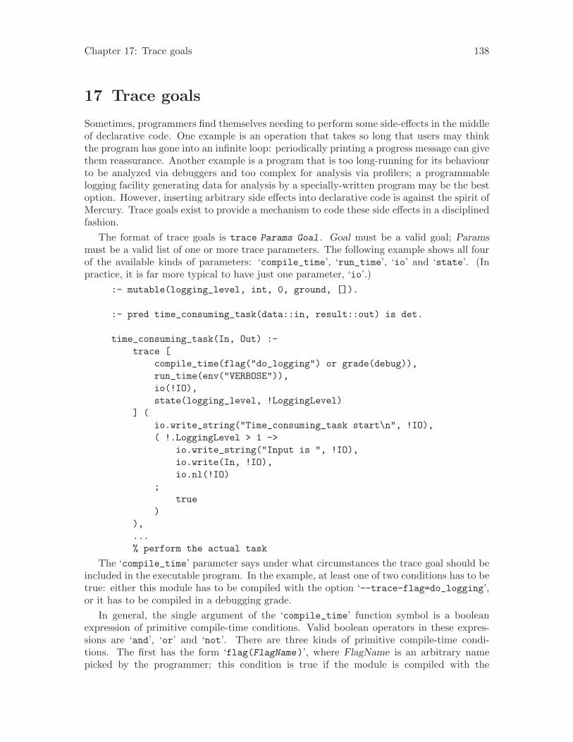
Chapter 17: Trace goals 138
17 Trace goals
Sometimes, programmers find themselves needing to perform some side-effects in the middleof declarative code. One example is an operation that takes so long that users may thinkthe program has gone into an infinite loop: periodically printing a progress message can givethem reassurance. Another example is a program that is too long-running for its behaviourto be analyzed via debuggers and too complex for analysis via profilers; a programmablelogging facility generating data for analysis by a specially-written program may be the bestoption. However, inserting arbitrary side effects into declarative code is against the spirit ofMercury. Trace goals exist to provide a mechanism to code these side effects in a disciplinedfashion.
The format of trace goals is trace Params Goal . Goal must be a valid goal; Paramsmust be a valid list of one or more trace parameters. The following example shows all fourof the available kinds of parameters: ‘compile_time’, ‘run_time’, ‘io’ and ‘state’. (Inpractice, it is far more typical to have just one parameter, ‘io’.)
:- mutable(logging_level, int, 0, ground, []).
:- pred time_consuming_task(data::in, result::out) is det.
time_consuming_task(In, Out) :-
trace [
compile_time(flag("do_logging") or grade(debug)),
run_time(env("VERBOSE")),
io(!IO),
state(logging_level, !LoggingLevel)
] (
io.write_string("Time_consuming_task start\n", !IO),
( !.LoggingLevel > 1 ->
io.write_string("Input is ", !IO),
io.write(In, !IO),
io.nl(!IO)
;
true
)
),
...
% perform the actual task
The ‘compile_time’ parameter says under what circumstances the trace goal should beincluded in the executable program. In the example, at least one of two conditions has to betrue: either this module has to be compiled with the option ‘--trace-flag=do_logging’,or it has to be compiled in a debugging grade.
In general, the single argument of the ‘compile_time’ function symbol is a booleanexpression of primitive compile-time conditions. Valid boolean operators in these expres-sions are ‘and’, ‘or’ and ‘not’. There are three kinds of primitive compile-time condi-tions. The first has the form ‘flag(FlagName)’, where FlagName is an arbitrary namepicked by the programmer; this condition is true if the module is compiled with the
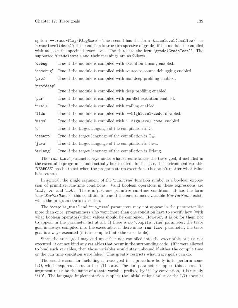
Chapter 17: Trace goals 139
option ‘--trace-flag=FlagName ’. The second has the form ‘tracelevel(shallow)’, or‘tracelevel(deep)’; this condition is true (irrespective of grade) if the module is compiledwith at least the specified trace level. The third has the form ‘grade(GradeTest)’. Thesupported ‘GradeTests’s and their meanings are as follows.
‘debug’ True if the module is compiled with execution tracing enabled.
‘ssdebug’ True if the module is compiled with source-to-source debugging enabled.
‘prof’ True if the module is compiled with non-deep profiling enabled.
‘profdeep’True if the module is compiled with deep profiling enabled.
‘par’ True if the module is compiled with parallel execution enabled.
‘trail’ True if the module is compiled with trailing enabled.
‘llds’ True if the module is compiled with ‘--highlevel-code’ disabled.
‘mlds’ True if the module is compiled with ‘--highlevel-code’ enabled.
‘c’ True if the target language of the compilation is C.
‘csharp’ True if the target language of the compilation is C#.
‘java’ True if the target language of the compilation is Java.
‘erlang’ True if the target language of the compilation is Erlang.
The ‘run_time’ parameter says under what circumstances the trace goal, if included inthe executable program, should actually be executed. In this case, the environment variable‘VERBOSE’ has be to set when the program starts execution. (It doesn’t matter what valueit is set to.)
In general, the single argument of the ‘run_time’ function symbol is a boolean expres-sion of primitive run-time conditions. Valid boolean operators in these expressions are‘and’, ‘or’ and ‘not’. There is just one primitive run-time condition. It has the form‘env(EnvVarName)’, this condition is true if the environment variable EnvVarName existswhen the program starts execution.
The ‘compile_time’ and ‘run_time’ parameters may not appear in the parameter listmore than once; programmers who want more than one condition have to specify how (withwhat boolean operators) their values should be combined. However, it is ok for them notto appear in the parameter list at all. If there is no ‘compile_time’ parameter, the tracegoal is always compiled into the executable; if there is no ‘run_time’ parameter, the tracegoal is always executed (if it is compiled into the executable).
Since the trace goal may end up either not compiled into the executable or just notexecuted, it cannot bind any variables that occur in the surrounding code. (If it were allowedto bind such variables, then those variables would stay unbound if either the compile timeor the run time condition were false.) This greatly restricts what trace goals can do.
The usual reason for including a trace goal in a procedure body is to perform someI/O, which requires access to the I/O state. The ‘io’ parameter supplies this access. Itsargument must be the name of a state variable prefixed by ‘!’; by convention, it is usually‘!IO’. The language implementation supplies the initial unique value of the I/O state as
Chapter 17: Trace goals 140
the value of ‘!.IO’ at the start of the trace goal; it requires the trace goal to give back thefinal unique value of the I/O state as the value of ‘!.IO’ current at the end of the tracegoal.
Note that trace goals that wish to do I/O must include this parameter in their parameterlist even if the surrounding code already has access to an I/O state. This is becauseotherwise, doing any I/O inside the trace goal would destroy the value of the current I/Ostate, changing the instantiation state of the variable holding it, and trace goals are notallowed to do that.
The ‘io’ parameter may appear in the parameter list at most once, since it doesn’t makesense to have two copies of the I/O state available to the trace goal.
Besides doing I/O, trace goals may read and possibly write the values of mutable vari-ables. Each mutable the trace goal wants access to should be listed in its own ‘state’ pa-rameter (which may therefore appear in the parameter list more than once). Each ‘state’parameter has two arguments: the first gives the name of the mutable, while the secondmust be the name of a state variable prefixed by ‘!’, e.g. ‘!LoggingLevel’. The lan-guage implementation supplies the initial value of the mutable as the value of (in this case)‘!.LoggingLevel’ at the start of the trace goal; at the end of the trace goal, it puts thevalue of ‘!.LoggingLevel’ current then back into the mutable.
The intention here is that trace goals should be able to access mutables that give theminformation about the parameters within which they should operate. The ability of tracegoals to actually update the values of mutables is intended to allow the implementationof trace goals whose actions depend on the actions executed by previous trace goals. Forexample, a trace goal could test whether the current input value is the same as the previousinput value, and if it is, then it can say so instead of printing the value out again. Anotherpossibility is a progress message which is printed not for every item processed, but for every1000th item, reassuring users without overwhelming them with a deluge of output.
This kind of code is the only intended use of this ability. Any program in which the valueof a mutable set by a trace goal is inspected by code that is not itself within a trace goalis explicitly violating the intended uses of trace goals. Only the difficulty of implementingthe required global program analysis prevents the language design from outlawing suchprograms in the first place.
The compiler will not delete trace goals from the bodies of the procedures containingthem. However, trace goals inside a procedure don’t prevent calls to that procedure frombeing optimized away, if such optimization is otherwise possible. (There is no point indebugging or logging operations that don’t actually occur.) In their effect on programoptimizations, trace goals function as a kind of impure code, but one with an implicitpromise pure around the clause in which they occur.

Chapter 18: Pragmas 141
18 Pragmas
The pragma declarations described below are a standard part of the Mercury language,as are the pragmas for controlling the foreign language interface (see Chapter 14 [For-eign language interface], page 97) and impurity (see Chapter 15 [Impurity], page 128).As an extension, implementations may also choose to support additional pragmas withimplementation-dependent semantics (see Chapter 19 [Implementation-dependent exten-sions], page 145).
18.1 Inlining
A declaration of the form
:- pragma inline(Name/Arity).
is a hint to the compiler that all calls to the predicate(s) or function(s) with name Nameand arity Arity should be inlined.
The current Mercury implementation is smart enough to inline simple predicates evenwithout this hint.
A declaration of the form
:- pragma no_inline(Name/Arity).
ensures the compiler will not inline this predicate. This may be used simply for performanceconcerns (inlining can cause unwanted code bloat in some cases) or to prevent possiblydangerous inlining when using low-level C code.
18.2 Type specialization
The overhead of polymorphism can in some cases be significant, especially where poly-morphic predicates make heavy use of class method calls or the builtin unification andcomparison routines. To avoid this, the programmer can suggest to the compiler that aspecialized version of a procedure should be created for a specific set of argument types.
18.2.1 Syntax and semantics of type specialization pragmas
A declaration of the form
:- pragma type_spec(Name/Arity, Subst).
:- pragma type_spec(Name(Modes), Subst).
suggests to the compiler that a specialized version of predicate(s) or function(s) with nameName and arity Arity should be created with the type substitution given by Subst appliedto the argument types. The second form of the declaration only suggests specialization ofthe specified mode of the predicate or function.
The substitution is written as a conjunction of bindings of the form ‘TypeVar = Type ’,for example ‘K = int’ or ‘(K = int, V = list(int))’.
The declarations
:- pred map.lookup(map(K, V), K, V).
:- pragma type_spec(map.lookup/3, K = int).
give a hint to the compiler that a version of ‘map.lookup/3’ should be created for integerkeys.
Chapter 18: Pragmas 142
Implementations are free to ignore ‘pragma type_spec’ declarations. Implementationsare also free to perform type specialization even in the absence of any ‘pragma type_spec’declarations.
18.2.2 When to use type specialization
The set of types for which a predicate or function should be specialized is best determinedby profiling your application. Overuse of type specialization will result in code bloat.
Type specialization of predicates or functions which unify or compare polymorphic vari-ables is most effective when the specialized types are builtin types such as int, float andstring, or enumeration types, since their unification and comparison procedures are simpleand can be inlined.
Predicates or functions which make use of type class method calls may also be candidatesfor specialization. Again, this is most effective when the called type class methods are simpleenough to be inlined.
18.2.3 Implementation specific details
The Melbourne Mercury compiler performs user-requested type specializations when in-voked with ‘--user-guided-type-specialization’, which is enabled at optimization level‘-O2’ or higher. However, for the Java back-end, user-requested type specializations are ig-nored.
18.3 Obsolescence
Declarations of the forms
:- pragma obsolete(Name/Arity).
:- pragma obsolete(Name/Arity,
[ReplName1/ReplArity1, ..., ReplNameN/ReplArityN]).
declare that the predicate(s) or function(s) with name Name and arity Arity are “obsolete”:they instruct the compiler to issue a warning whenever the named predicate(s) and/orfunction(s) are used. The second form tells the compiler to suggest the use of one of thelisted possible replacements.
Declarations of the forms
:- pragma obsolete_proc(PredName(ArgMode1, ..., ArgModeN)).
:- pragma obsolete_proc(PredName(ArgMode1, ..., ArgModeN),
[ReplName1/ReplArity1, ..., ReplNameN/ReplArityN]).
:- pragma obsolete_proc(FuncName(ArgMode1, ..., ArgModeN) = RetMode).
:- pragma obsolete_proc(FuncName(ArgMode1, ..., ArgModeN) = RetMode,
[ReplName1/ReplArity1, ..., ReplNameN/ReplArityN]).
similarly declare that the predicate named PredName with arity N, or the function namedFuncName with arity N, is obsolete when called in the specified mode. These forms alsoallow the specification of an optional list of possible replacements.
These declarations are intended for use by library developers, to allow gradual (ratherthan abrupt) evolution of library interfaces. If a library developer changes the interface ofa library predicate or procedure, they should leave its old version in the library, but mark itas obsolete using one of these declarations, and document how library users should modify

Chapter 18: Pragmas 143
their code to suit the new interface. The users of the library will then get a warning if theyuse obsolete features, and can consult the library documentation to determine how to fixtheir code. Eventually, when the library developer believes that users have had sufficientwarning, they can remove the old version entirely.
18.4 No determinism warnings
A declaration of the form
:- pragma no_determinism_warning(Name/Arity).
tells the compiler not to generate any warnings that the determinism declarations of pro-cedures of the predicate or function with name Name and arity Arity are not as tight asthey could be.
‘pragma no_determinism_warning’ declarations are intended for use in situations inwhich the code of a predicate has one determinism, but the declared determinism of theprocedure must be looser due to some outside requirement. One such situation is when aset of procedures are all possible values of the same higher-order variable, which requiresthem to have the same argument types, modes, and determinisms. If (say) most of theprocedures are det but some are erroneous (that is, they always throws an exception), theprocedures that are declared det but whose bodies have determinism erroneous will geta warning saying their determinism declaration could be tighter, unless the programmerspecifies this pragma for them.
18.5 No dead predicate warnings
A declaration of the form
:- pragma consider_used(Name/Arity).
tells the compiler to consider the predicate or function with name Name and arity Arity tobe used, and not generate any dead procedure/predicate/function warnings either for thenamed predicate, or for the other predicates and functions that it calls, either directly orindirectly.
‘pragma consider_used’ declarations are intended for use in situations in which thecode that was intended to call such a predicate or function is not yet written.
18.6 Source file name
The ‘source_file’ pragma and ‘#line ’ directives provide support for preprocessors andother tools that generate Mercury code. The tool can insert these directives into the gener-ated Mercury code to allow the Mercury compiler to report diagnostics (error and warningmessages) at the original source code location, rather than at the location in the automat-ically generated Mercury code.
A ‘source_file’ pragma is a declaration of the form
:- pragma source_file(Name).
where Name is a string that specifies the name of the source file.
For example, if a preprocessor generated a file ‘foo.m’ based on a input file ‘foo.m.in’,and it copied lines 20, 30, and 31 from ‘foo.m.in’, the following directives would ensurethat any error or warnings for those lines copied from ‘foo.m’ were reported at their originalsource locations in ‘foo.m.in’.

Chapter 18: Pragmas 144
:- module foo.
:- pragma source_file("foo.m.in").
#20
% this line comes from line 20 of foo.m
#30
% this line comes from line 30 of foo.m
% this line comes from line 31 of foo.m
:- pragma source_file("foo.m").
#10
% this automatically generated line is line 10 of foo.m
Note that if a generated file contains some text which is copied from a source file, andsome which is automatically generated, it is a good idea to use ‘pragma source_file’and ‘#line ’ directives to reset the source file name and line number to point back to thegenerated file for the automatically generated text, as in the above example.

Chapter 19: Implementation-dependent extensions 145
19 Implementation-dependent extensions
The Melbourne Mercury implementation supports the following extensions to the Mercurylanguage:
19.1 Fact tables
Large tables of facts can be compiled using a different algorithm that is more efficient andcan produce more efficient code.
A declaration of the form
:- pragma fact_table(Name/Arity, FileName).
tells the compiler that the predicate or function with name Name and arity Arity is definedby a set of facts in an external file FileName. Defining large tables of facts in this way allowsthe compiler to use a more efficient algorithm for compiling them. This algorithm uses lessmemory than would normally be required to compile the facts, so much larger tables arepossible.
Each mode is indexed on all its input arguments so the compiler can produce veryefficient code using this technique.
In the current implementation, the table of facts is compiled into a separate C file named‘FileName.c’. The compiler will automatically generate the correct dependencies for thisfile when the command ‘mmake main_module.depend’ is invoked. This ensures that the Cfile will be compiled to ‘FileName.o’ and then linked with the other object files when ‘mmakemain_module ’ is invoked.
The main limitation of the ‘fact_table’ pragma is that in the current implementation,predicates or functions defined as fact tables can only have arguments of types string, intor float.
Another limitation is that the ‘--high-level-code’ back-end does not support ‘pragmafact_table’ for procedures with determinism nondet or multi.
19.2 Tabled evaluation
(Note: “Tabled evaluation” has no relation to the “fact tables” described above.)
Ordinarily, the results of each procedure call are not recorded; if the same procedure iscalled with the same arguments, then the answer(s) must be recomputed again. For someprocedures, this recomputation can be very wasteful.
With tabled evaluation, the implementation keeps a table containing the previouslycomputed results of the specified procedure; this table is sometimes called the memo table(since it “remembers” previous answers). At each procedure call, the implementation willsearch the memo table to check whether the answer(s) have already been computed, and ifso, the answers will be returned directly from the memo table rather than being recomputed.This can result in much faster execution, at the cost of additional space to record answersin the table.
The implementation can also check at runtime for the situation where a procedure callsitself recursively with the same arguments, which would normally result in a infinite loop;

Chapter 19: Implementation-dependent extensions 146
if this situation is encountered, it can (at the programmer’s option) either throw an excep-tion, or avoid the infinite loop by computing solutions using a “minimal model” semantics.(Specifically, the minimal model computed by our implementation is the perfect model.)
The current Mercury implementation supports three different pragmas for tabling, tocover these three cases: ‘loop_check’, ‘memo’, and ‘minimal_model’.
• The ‘loop_check’ pragma asks only for loop checking. With this pragma, the memotable will map each distinct set of input arguments only to a single boolean sayingwhether a call with those arguments is currently active or not; the pragma’s only effectis to cause the predicate to throw an exception if this boolean says that the current callhas the same arguments as one of its ancestors, which indicates an infinite recursiveloop.
Note that loop checking for nondet and multi predicates assumes that calls to thesepredicates generate all their solutions and then fail. If a caller asks them only for somesolutions and then cuts away all later solutions (e.g. via a quantification that only askswhether a solution satisfying a particular test exists), then the cut-away call never getsa chance to record the fact that it is not longer active. The next call to that predicatewith the same arguments will therefore think that the previous call is still active, andwill consider this call to be an infinite loop.
• The ‘memo’ pragma asks for both loop checking and memoization. With this pragma,the memo table will map each distinct set of input arguments either to the set ofresults computed previously for those arguments, or to an indication that the call isstill active and thus those results are still being computed. This predicate will thus lookfor infinite recursive loops (and throw an exception if and when it finds one) but it willalso record all its solutions in the memo table, and will avoid recomputing solutionsthat are already available in the memo table.
• The ‘minimal_model’ pragma asks for the computation of a “minimal model” seman-tics. These differ from the ‘memo’ pragma in that the detection of what appears to bean infinite recursive loop is not fatal. The implementation will consider the apparentlyinfinitely recursive calls to fail if the call concerned has no way of computing any solu-tions it has not already computed and recorded, and if it does have such a way, thenit switches the execution to explore those ways before coming back to the apparentlyinfinitely recursive call.
Minimal model evaluation is applicable only to procedures that can succeed more thanonce, and only in grades that explicitly support it.
The syntax for each of these declarations is
:- pragma memo(Name/Arity).
:- pragma memo(Name/Arity, [list of tabling attributes]).
:- pragma loop_check(Name/Arity).
:- pragma loop_check(Name/Arity, [list of tabling attributes]).
:- pragma minimal_model(Name/Arity).
:- pragma minimal_model(Name/Arity, [list of tabling attributes]).
where Name/Arity specifies the predicate or function to which the declaration applies. Thedeclaration applies to all modes of the predicate and/or function named. At most one ofthese declarations may be specified for any given predicate or function.
Chapter 19: Implementation-dependent extensions 147
Programmers can also request the application of tabling only to one particular mode ofa predicate or function, via declarations such as these:
:- pragma memo(Name(in, in, out)).
:- pragma memo(Name(in, in, out), [list of tabling attributes]).
:- pragma loop_check(Name(in, out)).
:- pragma loop_check(Name(in, out), [list of tabling attributes]).
:- pragma minimal_model(Name(in, in, out, out)).
:- pragma minimal_model(Name(in, in, out, out), [list of tabling attributes]).
Because all variants of tabling record the values of input arguments, and all except‘loop_check’ also record the values of output arguments, you cannot apply any of thesepragmas to procedures whose arguments’ modes include any unique component.
Tabled evaluation of a predicate or function that has an argument whose type is aforeign type will result in a run-time error unless the foreign type is one for which the‘can_pass_as_mercury_type’ and ‘stable’ assertions have been made (see Section 14.4[Using foreign types from Mercury], page 108).
The optional list of attributes allows programmers to control some aspects of the man-agement of the memo table(s) of the procedure(s) affected by the pragma.
The ‘allow_reset’ attribute asks the compiler to define a predicate that, when called,resets the memo table. The name of this predicate will be “table reset for”, followed by thename of the tabled predicate, followed by its arity, and (if the predicate has more than onemode) by the mode number (the first declared mode is mode 0, the second is mode 1, andso on). These three or four components are separated by underscores. The reset predicatetakes a di/uo pair of I/O states as arguments. The presence of these I/O state argumentsin the reset predicate, and the fact that tabled predicates cannot have unique argumentstogether imply that a memo table cannot be reset while a call using that memo table isactive.
The ‘statistics’ attribute asks the compiler to define a predicate that, whencalled, returns statistics about the memo table. The name of this predicate will be“table statistics for”, followed by the name of the tabled predicate, followed by its arity,and (if the predicate has more than one mode) by the mode number (the first declaredmode is mode 0, the second is mode 1, and so on). These three or four components areseparated by underscores. The statistics predicate takes three arguments. The second andthird are a di/uo pair of I/O states, while the first is an output argument that containsinformation about accesses to and modifications of the procedure’s memo table, both sincethe creation of the table, and since the last call to this predicate. The type of this argumentis defined in the file table builtin.m in the Mercury standard library. That module alsocontains a predicate for printing out this information in a programmer-friendly format.
The remaining two attributes, ‘fast_loose’ and ‘specified’, control how argumentsare looked up in the memo table. The default implementation looks up the value of eachinput argument, and thus requires time proportional to the number of function symbols inthe input arguments. This is the only implementation allowed for minimal model tabling,but for predicates tabled with the ‘loop_check’ and ‘memo’ pragmas, programmers can alsochoose some other tabling methods.
The ‘fast_loose’ attribute asks the compiler to generate code that looks up only the ad-dress of each input argument in the memo table, which means that the time required is linear

Chapter 19: Implementation-dependent extensions 148
only in the number of input arguments, not their size. The tradeoff is that ‘fast_loose’does not recognize calls as duplicates if they involve input arguments that are logicallyequal but are stored at different locations in memory. The following declaration calls forthis variant of tabling.
:- pragma memo(Name(in, in, in, out),
[allow_reset, statistics, fast_loose]).
The ‘specified’ attribute allows programmers to choose individually, for each inputargument, whether that argument should be looked up in the memo table by value or byaddress, or whether it should be looked up at all:
:- pragma memo(Name(in, in, in, out), [allow_reset, statistics,
specified([value, addr, promise_implied, output])]).
The ‘specified’ attribute should have an argument which is a list, and this list shouldcontain one element for each argument of the predicate or function concerned (if a func-tion, the last element is for the return value). For output arguments, the list elementshould be ‘output’. For input arguments, the list element may be ‘value’, ‘addr’ or‘promise_implied’. The first calls for tabling the argument by value, the second callsfor tabling the argument by address, and the third calls for not tabling the argument atall. This last course of action promises that any two calls that agree on the values of thevalue-tabled input arguments and on the addresses of the address-tabled input argumentswill behave the same regardless of the values of the untabled input arguments. In mostcases, this will mean that the values of the untabled arguments are implied by the valuesof the value-tabled arguments and the addresses of the address-tabled arguments, thoughthe promise can also be fulfilled if the table predicate or function does not actually use theuntabled argument for computing any of its output. (It is ok for it to use the untabledargument to decide what exception to throw.)
If the tabled predicate or function has only one mode, then this declaration can also bespecified without giving the argument modes:
:- pragma memo(Name/Arity, [allow_reset, statistics,
specified([value, addr, promise_implied, output])]).
Note that a ‘pragma minimal_model’ declaration changes the declarative semantics ofthe specified predicate or function: instead of using the completion of the clauses as thebasis for the semantics, as is normally the case in Mercury, the declarative semantics thatis used is a “minimal model” semantics, specifically, the perfect model semantics. Anythingwhich is true or false in the completion semantics is also true or false (respectively) inthe perfect model semantics, but there are goals for which the perfect model specifies thatthe result is true or false, whereas the completion semantics leaves the result unspecified.For these goals, the usual Mercury semantics requires the implementation to either loop orreport an error message, but the perfect model semantics requires a particular answer tobe returned. In particular, the perfect model semantics says that any call that is not truein all models is false.
Programmers should therefore use a ‘pragma minimal_model’ declaration only in caseswhere their intended interpretation for a procedure coincides with the perfect model forthat procedure. Fortunately, however, this is usually what programmers intend.
For more information on tabling, see K. Sagonas’s PhD thesis The SLG-WAM: A Search-Efficient Engine for Well-Founded Evaluation of Normal Logic Programs. See [[4]], page 158.

Chapter 19: Implementation-dependent extensions 149
The operational semantics of procedures with a ‘pragma minimal_model’ declaration cor-responds to what Sagonas calls “SLGd resolution”.
In the general case, the execution mechanism required by minimal model tabling is quitecomplicated, requiring the ability to delay goals and then wake them up again. The Mercuryimplementation uses a technique based on copying relevant parts of the stack to the heapwhen delaying goals. It is described in Tabling in Mercury: design and implementation byZ. Somogyi and K. Sagonas, Proceedings of the Eight International Symposium on PracticalAspects of Declarative Languages.� �
Please note: the current implementation of tabling does not support all the possiblecompilation grades (see the “Compilation model options” section of the Mercury User’sGuide) allowed by the Mercury implementation. In particular, minimal model tabling isincompatible with high level code and the use of trailing. 19.3 Termination analysis
The compiler includes a termination analyser which can be used to prove termination ofpredicates and functions. Details of the analysis is available in “Termination Analysis forMercury” by Chris Speirs, Zoltan Somogyi and Harald Sondergaard. See [[1]], page 158.
The analysis is based on an algorithm proposed by Gerhard Groger and Lutz Plumerin their paper “Handling of mutual recursion in automatic termination proofs for logicprograms.” See [[2]], page 158.
For an introduction to termination analysis for logic programs, please refer to “Termi-nation Analysis for Logic Programs” by Chris Speirs. See [[3]], page 158.
Information about the termination properties of a predicate or function can be given tothe compiler. Pragmas are also available to require the compiler to prove termination of agiven predicate or function, or to give an error message if it cannot do so.
The analyser is enabled by the option ‘--enable-termination’, which can be abbrevi-ated to ‘--enable-term’. When termination analysis is enabled, any predicates or functionswith a ‘check_termination’ pragma defined on them will have their termination checked,and if termination cannot be proved, the compiler will emit an error message detailing thereason that termination could not be proved.
The option ‘--check-termination’, which may be abbreviated to ‘--check-term’ or‘--chk-term’, forces the compiler to check the termination of all predicates in the module.It is common for the compiler to be unable to prove termination of some predicates andfunctions because they call other predicates which could not be proved to terminate orbecause they use language features (such as higher-order calls) which cannot be usefullyanalysed. In this case, the compiler only emits a warning for these predicates and functionsif the ‘--verbose-check-termination’ option is enabled. For every predicate or functionthat the compiler cannot prove the termination of, a warning message is emitted, but compi-lation continues. The ‘--check-termination’ option implies the ‘--enable-termination’option.
The accuracy of the termination analysis is substantially degraded if intermodule op-timization is not enabled. Unless intermodule optimization is enabled, the compiler mustassume that any imported predicate may not terminate.

Chapter 19: Implementation-dependent extensions 150
By default, the compiler assumes that a procedure defined using the foreign languageinterface will terminate for all input if it does not call Mercury. If it does call Mercury thenby default the compiler will assume that it may not terminate.
The foreign code attributes ‘terminates’/‘does_not_terminate’ may be used to forcethe compiler to treat a foreign proc as terminating/non-terminating irrespective of whetherit calls Mercury. As a matter of style, it is preferable to use foreign code attributes forforeign procs rather than the termination pragmas described below.
The following declarations can be used to inform the compiler of the termination prop-erties of a predicate or function.
:- pragma terminates(Name/Arity).
This declaration may be used to inform the compiler that this predicate or functionis guaranteed to terminate for any input. This is useful when the compiler cannot provetermination of some predicates or functions which are in turn preventing the compiler fromproving termination of other predicates or functions. This declaration affects not only thepredicate specified but also any other predicates that are mutually recursive with it.
:- pragma does_not_terminate(Name/Arity).
This declaration may be used to inform the compiler that this predicate may not termi-nate. This declaration affects not only the predicate specified but also any other predicatesthat are mutually recursive with it.
:- pragma check_termination(Name/Arity).
This pragma forces the compiler to prove termination of this predicate. If it cannot provethe termination of the specified predicate or function, then the compiler will quit with anerror message.
19.4 Feature sets
The Melbourne Mercury implementation supports a number of optional compilation modelfeatures, such as Section 19.5 [Trailing], page 151 or Section 19.2 [Tabled evaluation],page 145. Feature sets allow the programmer to assert that a module requires the presenceof one or more optional features in the compilation model. These assertions can be madeusing a ‘pragma require_feature_set’ declaration.
The ‘require_feature_set’ pragma declaration has the following form:
:- pragma require_feature_set(Features).
where Features is a (possibly empty) list of features.
The supported features are:
‘concurrency’This specifies that the compilation model must support concurrent executionof multiple threads.
‘single_prec_float’This specifies that the compilation model must use single precision floats. Thisfeature cannot be specified together with the ‘double_prec_float’ feature.
Chapter 19: Implementation-dependent extensions 151
‘double_prec_float’,This feature specifies tha the compilation model must use double precisionfloats. This feature cannot be specified together with the ‘single_prec_float’feature.
‘memo’ This feature specifies that the compilation model must support memoisation(see Section 19.2 [Tabled evaluation], page 145).
‘parallel_conj’This feature specifies that the compilation model must support parallel ex-ecution of conjunctions. This feature cannot be specified together with the‘trailing’ feature.
‘trailing’This feature specifies that the compilation model must support trailing, seeSection 19.5 [Trailing], page 151. This feature cannot be specified togetherwith the ‘parallel_conj’ feature.
‘strict_sequential’This feature specifies that a semantics that is equivalent to the strict sequentialoperational semantics must be used.
‘conservative_gc’This feature specifies that a module requires conservative garbage collection.This feature is only checked when using the C backends; it is ignored by thenon-C backends.
When a module containing a ‘pragma require_feature_set’ declaration is compiled,the implementation checks to see that the specified features are supported by the compila-tion model. It emits an error if they are not.
A ‘pragma require_feature_set’ may only occur in the implementation section of amodule.
A ‘pragma require_feature_set’ affects only the module in which it occurs; in partic-ular it does not affect any submodules.
If a module contains multiple ‘pragma require_feature_set’ declarations, then theimplementation should emit an error if any of them specifies a feature that is not supportedby the compilation model.
19.5 Trailing
In certain compilation grades (see the “Compilation model options” section of the MercuryUser’s Guide), the Melbourne Mercury implementation supports trailing. Trailing is ameans of having side-effects, such as destructive updates to data structures, undone onbacktracking. The basic idea is that during forward execution, whenever you perform adestructive modification to a data structure that may still be live on backtracking, youshould record whatever information is necessary to restore it on a stack-like data structurecalled the “trail”. Then, if a computation fails, and execution backtracks to before thoseupdates were performed, the Mercury runtime engine will traverse the trail back to themost recent choice point, undoing all those updates.
Chapter 19: Implementation-dependent extensions 152
The interface used is a set of C functions (which are actually implemented as macros)and types. Typically these will be called from C code within ‘pragma foreign_proc’ or‘pragma foreign_code’ declarations in Mercury code.
For an example of the use of this interface, see the module ‘extras/trailed_update/tr_array.m’in the Mercury extras distribution.
19.5.1 Choice points
A “choice point” is a point in the computation to which execution might backtrack whena goal fails or throws an exception. The “current” choice point is the one that was mostrecently encountered; that is also the one to which execution will branch if the currentcomputation fails.
When you trail an update, the Mercury engine will ensure that if execution ever back-tracks to the choice point that was current at the time of trailing, then the update will beundone.
If the Mercury compiler determines that it will never need to backtrack to a particularchoice point, then it will “prune” away that choice point. If a choice point is pruned, thetrail entries for those updates will not necessarily be discarded, because in general they maystill be necessary in case we backtrack to a prior choice point.
19.5.2 Value trailing
The simplest form of trailing is value trailing. This allows you to trail updates to memoryand have the Mercury runtime engine automatically undo them on backtracking.
• MR_trail_value()
Prototype:
void MR_trail_value(MR_Word *address, MR_Word value);
Ensures that if future execution backtracks to the current choice point, thenvalue will be placed in address.
• MR_trail_current_value()
Prototype:
void MR_trail_current_value(MR_Word *address);
Ensures that if future execution backtracks to the current choice point, thevalue currently in address will be restored.
‘MR_trail_current_value(address)’ is equivalent to ‘MR_trail_value(address,*address)’.
Note that address must be word aligned for both MR_trail_current_value() and MR_
trail_value(). (The address of Mercury data structures that have been passed to C viathe foreign language interface are guaranteed to be appropriately aligned.)
19.5.3 Function trailing
For more complicated uses of trailing, you can store the address of a C function on thetrail and have the Mercury runtime call your function back whenever future executionbacktracks to the current choice point or earlier, or whenever that choice point is pruned,

Chapter 19: Implementation-dependent extensions 153
because execution commits to never backtracking over that point, or whenever that choicepoint is garbage collected.
Note the garbage collector in the current Mercury implementation does not garbage-collect the trail; this case is mentioned only so that we can cater for possible future exten-sions.
• MR_trail_function()
Prototype:
typedef enum {
MR_undo,
MR_exception,
MR_retry,
MR_commit,
MR_solve,
MR_gc
} MR_untrail_reason;
void MR_trail_function(
void (*untrail_func)(void *, MR_untrail_reason),
void *value
);
A call to ‘MR_trail_function(untrail_func, value)’ adds an entry to thefunction trail. The Mercury implementation ensures that if future executionever backtracks to the current choicepoint, or backtracks past the current choi-cepoint to some earlier choicepoint, then (*untrail_func)(value, reason)
will be called, where reason will be ‘MR_undo’ if the backtracking was due toa goal failing, ‘MR_exception’ if the backtracking was due to a goal throw-ing an exception, or ‘MR_retry’ if the backtracking was due to the use of the“retry” command in ‘mdb’, the Mercury debugger, or any similar user requestin a debugger. The Mercury implementation also ensures that if the currentchoice point is pruned because execution commits to never backtracking toit, then (*untrail_func)(value, MR_commit) will be called. It also ensuresthat if execution requires that the current goal be solvable, then (*untrail_
func)(value, MR_solve) will be called. This happens in calls to solutions/2,for example. (MR_commit is used for “hard” commits, i.e. when we commit to asolution and prune away the alternative solutions; MR_solve is used for “soft”commits, i.e. when we must commit to a solution but do not prune away all thealternatives.)
MR gc is currently not used — it is reserved for future use.
Typically if the untrail func is called with reason being ‘MR_undo’, ‘MR_exception’, or‘MR_retry’, then it should undo the effects of the update(s) specified by value, and then freeany resources associated with that trail entry. If it is called with reason being ‘MR_commit’or ‘MR_solve’, then it should not undo the update(s); instead, it may check for floundering(see the next section). In the ‘MR_commit’ case it may, in some cases, be possible to also freeresources associated with the trail entry. If it is called with anything else (such as ‘MR_gc’),then it should probably abort execution with an error message.
Chapter 19: Implementation-dependent extensions 154
Note that the address of the C function passed as the first argument of MR_trail_
function() must be word aligned.
19.5.4 Delayed goals and floundering
Another use for the function trail is check for floundering in the presence of delayed goals.
Often, when implementing certain kinds of constraint solvers, it may not be possible toactually solve all of the constraints at the time they are added. Instead, it may be necessaryto simply delay their execution until a later time, in the hope the constraints may becomesolvable when more information is available. If you do implement a constraint solver withthese properties, then at certain points in the computation — for example, after executinga negated goal — it is important for the system to check that there are no outstandingdelayed goals which might cause failure, before execution commits to this execution path.If there are any such delayed goals, the computation is said to “flounder”. If the check forfloundering was omitted, then it could lead to unsound behaviour, such as a negation failingeven though logically speaking it ought to have succeeded.
The check for floundering can be implemented using the function trail, by simply calling‘MR_trail_function()’ to add a function trail entry whenever you create a delayed goal,and putting the appropriate check for floundering in the ‘MR_commit’ and ‘MR_solve’ casesof your function. The Mercury extras distribution includes an example of this: see the‘ML_var_untrail_func()’ function in the file ‘extras/trailed_update/var.m’.) If yourfunction does detect floundering, then it should print an error message and then abortexecution.
19.5.5 Avoiding redundant trailing
If a mutable data structure is updated multiple times, and each update is recorded on thetrail using the functions described above, then some of this trailing may be redundant. Itis generally not necessary to record enough information to recover the original state of thedata structure for every update on the trail; instead, it is enough to record the originalstate of each updated data structure just once for each choice point occurring after the datastructure is allocated, rather than once for each update.
The functions described below provide a means to avoid redundant trailing.
• MR_ChoicepointId
Declaration:
typedef ... MR_ChoicepointId;
The type MR_ChoicepointId is an abstract type used to hold the identity of achoice point. Values of this type can be compared using C’s ‘==’ operator orusing ‘MR_choicepoint_newer()’.
• MR_current_choicepoint_id()
Prototype:
MR_ChoicepointId MR_current_choicepoint_id(void);
MR_current_choicepoint_id() returns a value indicating the identity of themost recent choice point; that is, the point to which execution would backtrack ifthe current computation failed. The value remains meaningful if the choicepoint
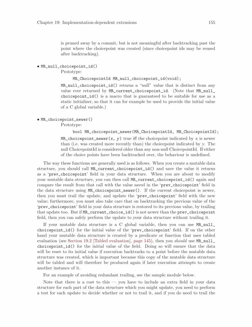
Chapter 19: Implementation-dependent extensions 155
is pruned away by a commit, but is not meaningful after backtracking past thepoint where the choicepoint was created (since choicepoint ids may be reusedafter backtracking).
• MR_null_choicepoint_id()
Prototype:
MR_ChoicepointId MR_null_choicepoint_id(void);
MR_null_choicepoint_id() returns a “null” value that is distinct from anyvalue ever returned by MR_current_choicepoint_id. (Note that MR_null_
choicepoint_id() is a macro that is guaranteed to be suitable for use as astatic initializer, so that it can for example be used to provide the initial valueof a C global variable.)
• MR_choicepoint_newer()
Prototype:
bool MR_choicepoint_newer(MR_ChoicepointId, MR_ChoicepointId);
MR_choicepoint_newer(x, y) true iff the choicepoint indicated by x is newerthan (i.e. was created more recently than) the choicepoint indicated by y. Thenull ChoicepointId is considered older than any non-null ChoicepointId. If eitherof the choice points have been backtracked over, the behaviour is undefined.
The way these functions are generally used is as follows. When you create a mutable datastructure, you should call MR_current_choicepoint_id() and save the value it returnsas a ‘prev_choicepoint’ field in your data structure. When you are about to modifyyour mutable data structure, you can then call MR_current_choicepoint_id() again andcompare the result from that call with the value saved in the ‘prev_choicepoint’ field inthe data structure using MR_choicepoint_newer(). If the current choicepoint is newer,then you must trail the update, and update the ‘prev_choicepoint’ field with the newvalue; furthermore, you must also take care that on backtracking the previous value of the‘prev_choicepoint’ field in your data structure is restored to its previous value, by trailingthat update too. But if MR_current_choice_id() is not newer than the prev_choicepointfield, then you can safely perform the update to your data structure without trailing it.
If your mutable data structure is a C global variable, then you can use MR_null_
choicepoint_id() for the initial value of the ‘prev_choicepoint’ field. If on the otherhand your mutable data structure is created by a predicate or function that uses tabledevaluation (see Section 19.2 [Tabled evaluation], page 145), then you should use MR_null_
choicepoint_id() for the initial value of the field. Doing so will ensure that the datawill be reset to its initial value if execution backtracks to a point before the mutable datastructure was created, which is important because this copy of the mutable data structurewill be tabled and will therefore be produced again if later execution attempts to createanother instance of it.
For an example of avoiding redundant trailing, see the sample module below.
Note that there is a cost to this — you have to include an extra field in your datastructure for each part of the data structure which you might update, you need to performa test for each update to decide whether or not to trail it, and if you do need to trail the
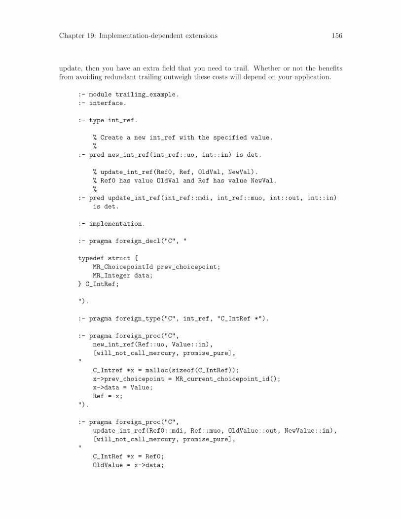
Chapter 19: Implementation-dependent extensions 156
update, then you have an extra field that you need to trail. Whether or not the benefitsfrom avoiding redundant trailing outweigh these costs will depend on your application.
:- module trailing_example.
:- interface.
:- type int_ref.
% Create a new int_ref with the specified value.
%
:- pred new_int_ref(int_ref::uo, int::in) is det.
% update_int_ref(Ref0, Ref, OldVal, NewVal).
% Ref0 has value OldVal and Ref has value NewVal.
%
:- pred update_int_ref(int_ref::mdi, int_ref::muo, int::out, int::in)
is det.
:- implementation.
:- pragma foreign_decl("C", "
typedef struct {
MR_ChoicepointId prev_choicepoint;
MR_Integer data;
} C_IntRef;
").
:- pragma foreign_type("C", int_ref, "C_IntRef *").
:- pragma foreign_proc("C",
new_int_ref(Ref::uo, Value::in),
[will_not_call_mercury, promise_pure],
"
C_Intref *x = malloc(sizeof(C_IntRef));
x->prev_choicepoint = MR_current_choicepoint_id();
x->data = Value;
Ref = x;
").
:- pragma foreign_proc("C",
update_int_ref(Ref0::mdi, Ref::muo, OldValue::out, NewValue::in),
[will_not_call_mercury, promise_pure],
"
C_IntRef *x = Ref0;
OldValue = x->data;

Chapter 19: Implementation-dependent extensions 157
/* Check whether we need to trail this update. */
if (MR_choicepoint_newer(MR_current_choicepoint_id(),
x->prev_choicepoint))
{
/*
** Trail both x->data and x->prev_choicepoint,
** since we’re about to update them both.
*/
assert(sizeof(x->data) == sizeof(MR_Word));
assert(sizeof(x->prev_choicepoint) == sizeof(MR_Word));
MR_trail_current_value((MR_Word *)&x->data);
MR_trail_current_value((MR_Word *)&x->prev_choicepoint);
/*
** Update x->prev_choicepoint to indicate that
** x->data’s previous value has been trailed
** at this choice point.
*/
x->prev_choicepoint = MR_current_choicepoint_id();
}
x->data = NewValue;
Ref = Ref0;
").

Chapter 20: Bibliography 158
20 Bibliography
[1]
Chris Speirs, Zoltan Somogyi and Harald Sondergaard, Termination Analysis for Mercury.In P. Van Hentenryck, editor, Static Analysis: Proceedings of the 4th International Sympo-sium, Lecture Notes in Computer Science. Springer, 1997. A longer version is available fordownload from http://www.mercurylang.org/documentation/papers/mu_97_09.ps.gz.
[2]
Gerhard Groger and Lutz Plumer, Handling of mutual recursion in automatic terminationproofs for logic programs. In K. Apt, editor, The Proceedings of the Joint InternationalConference and Symposium on Logic Programming, pages 336–350. MIT Press, 1992.
[3]
Chris Speirs, Termination Analysis for Logic Programs, Technical Report 97/23, Depart-ment of Computer Science, The University of Melbourne, Melbourne, Australia, 1997.Available from http://www.mercurylang.org/documentation/papers/mu_97_23.ps.gz.
[4]
K. Sagonas, The SLG-WAM: A Search-Efficient Engine for Well-Founded Evaluationof Normal Logic Programs, PhD thesis, SUNY at Stony Brook, 1996. Available fromhttp://user.it.uu.se/~kostis/Thesis/thesis.ps.gz.
[5]
B. Demoen and K. Sagonas, CAT: the Copying Approach to Tabling, In C. Palamidessi, H.Glaser and K. Meinke, editors, Principles of Declarative Programming, 10th InternationalSymposium, PLILP’98, Lecture Notes in Computer Science, Springer, 1998. Available formhttp://user.it.uu.se/~kostis/Papers/cat.ps.gz.