
Newton‘s Mechanics Stellar Orbits Gravity Leibniz Galilei Gaub1WS 2014/15.

The mechanics of marine sediment gravity flows
JEFFREY D. PARSONS*, CARL T. FRIEDRICHS†, PETER A. TRAYKOVSKI‡, DAVID MOHRIG§, JASIM IMRAN¶, JAMES P.M. SYVITSKI**, GARY PARKER††,
PERE PUIG‡‡, JAMES L. BUTTLES§ and MARCELO H. GARCÍA††
*School of Oceanography, University of Washington, Seattle, WA 98195, USA (Email: [email protected])†Virginia Institute of Marine Science, College of William & Mary, Gloucester Point, VA 23062, USA
‡Woods Hole Oceanographic Institution, Woods Hole, MA 02543, USA§Department of Earth, Atmospheric and Planetary Science, Massachusetts Institute of Technology, Cambridge, MA 02139, USA
¶Department of Civil and Environmental Engineering, University of South Carolina, Columbia, SC 29208, USA**Institute of Arctic and Alpine Research, University of Colorado, Boulder, CO 80309, USA
††Department of Civil and Environmental Engineering, University of Illinois, Urbana, IL 61801, USA‡‡Geologia Marina i Oceanografia Fisica, Institut de Ciencies del Mar, Barcelona E-08003, Spain
ABSTRACT
Sediment gravity flows, particularly those in the marine environment, are dynamically interestingbecause of the non-linear interaction of mixing, sediment entrainment/suspension and water-columnstratification. Turbidity currents, which are strongly controlled by mixing at their fronts, are thebest understood mode of sediment gravity flows. The type of mixing not only controls flow anddeposition near the front, but also changes the dynamics of turbidity currents flowing in self-formedchannels. Debris flows, on the other hand, mix little with ambient fluid. In fact, they have been shownto hydroplane, i.e. glide on a thin film of water. Hydroplaning enables marine debris flows to runoutmuch farther than their subaerial equivalents. Some sediment gravity flows require external energy,from sources such as surface waves. When these flows are considered as stratification-limited turbidity currents, models are able to predict observed downslope sediment fluxes. Most marinesediment gravity flows are supercritical and thus controlled by sediment supply to the water column.Therefore, the genesis of the flows is the key to their understanding and prediction. Virtually everysubaqueous failure produces a turbidity current, but they engage only a small percentage of theinitially failed material. Wave-induced resuspension can produce and sustain sediment gravity flows.Flooding rivers can also do this, but the complex interactions of settling and turbulence need to bebetter understood and measured to quantify this effect and document its occurrence. Ultimately,only integrative numerical models can connect these related phenomena, and supply realistic pre-dictions of the marine record.
Keywords Gravity flows, turbidity currents, debris flows, hydroplaning, fluid mud, sur-face waves.
INTRODUCTION
A sediment gravity flow is any flow by which sediment moves due to its contribution to the density of the surrounding fluid. Sediment gravityflows are not limited to the oceans, or even Earth.However, Earth’s oceans represent one of the bestplaces for observation of this unusual phenomenon.The oceans are particularly prone to sediment grav-
ity flows because the particle (sediment) density isgenerally of the same order of magnitude as, butstill larger than, the interstitial fluid. As a result,sediment gravity-flow deposits are ubiquitous in themarine sediment record. Reconstructing the attri-butes of the sediment record and tying those to theclimate at the time of deposition is fundamental tothe study of modern marine geology. In additionto palaeoclimate information contained within the
CMS_C06.qxd 4/27/07 9:18 AM Page 275

276 J.D. Parsons et al.
sediment record, marine stratigraphy is an impor-tant practical concern as the source for much of theworld’s remaining petroleum reserves.
Sediment gravity flows can be divided into five broad categories. Each flow type has a rangeof concentrations, Reynolds numbers, durationand grain size, which are summarized in Table 1.Submarine slides are large-scale mass-movementevents where particle–particle interactions are dom-inant and interstitial pore fluids play only a minorrole. Slides are primarily a result of tectonic forcesand cannot be easily treated with fluid-mechanical(continuum) models. They are most often studiedby geophysicists and geotechnical engineers andtheir characteristics have been summarized by Leeet al. (this volume, pp. 213–274). Debris flows arefast-moving masses of poorly sorted material whereparticle–particle interactions are important andrheology is a function of interstitial fluid pressureand internal friction. Debris flows are differentiatedfrom slides by their heightened internal deforma-tion and fluid-like properties. Turbidity currents aredilute mass concentrations (Cm < 10 kg m−3), fullyturbulent (Reynolds numbers Re > 104) flows ofpoorly sorted sediment. In addition to these threetraditional categories of sediment gravity flows, two have emerged recently. Commonly through-out this volume, these gravity flows are describedas ‘fluid muds’. However, mechanistically it iseasiest to divide them into wave-supported sedi-ment gravity flows and estuarine fluid muds.Wave-supported sediment gravity flows (WSSGF)require wave-induced resuspension for transport,
while estuarine fluid muds result from a con-vergence of sediment transport within an estuaryor sediment-rich shelf environment. Within thispaper, estuarine fluid muds are discussed in alimited manner, but have been summarized inWright & Friedrichs (2006).
Mention of the term sediment gravity flow, turbid-ity current or debris flow with regard to marinedeposits is virtually absent from the scientific literature prior to 1950. Flysch deposits, marine-derived sandstones interbedded with shale, havebeen studied since the nineteenth century, but their formative mechanisms were not understood untilKuenen & Migliorini (1950) linked turbidity cur-rents to these deposits. Turbidity currents gainedfurther recognition from an analysis of the 1929Grand Banks slope failure. Seagoing oceanographerssampled the deposit and mapped the bathymetryassociated with the slide. They proposed that a seismic event produced a turbidity current that trav-elled rapidly along the seafloor and broke several‘new’ transatlantic communication cables (Heezen& Ewing, 1952). The speed of front could be cal-culated because the timing of the cable breaks wasknown precisely. The speed was considerably fasterthan typical ocean currents (> 10 m s−1), indicatingthat a new type of current, driven by the negativebuoyancy resulting from the sediment itself, wasresponsible for the flow.
Petroleum geologists originally employed anci-ent analogues to interpret the sedimentary struc-ture of sandstone reservoirs because little wasknown about the bottom of the ocean. Later, a
Table 1 Categorization of different types of sediment gravity flows: Re is the relevant Reynolds numberdescribing the overall layer thickness
Type of flow Duration Speed Concentration Coarsest grain size Rheology Re(m s−1)
Submarine slide Minutes > 1? > 1000 kg m−3 Blocks (> 100 m3) Non-Newtonian? < 1Debris flow Minutes to hours 0.1–10 > 1000 kg m−3 Boulders (< 100 m3) Non-Newtonian < 100Estuarine fluid muds > Hours > 0.5 > 10 kg m−3 Silty sand Non-Newtonian < 100Wave-supported Hours 0.05–0.3 > 10 kg m−3 Sand Non-Newtonian? 1–104
sediment gravity flow
Turbidity current Minutes to days > 0.3 < 10 kg m−3 Coarse sand Newtonian > 104
CMS_C06.qxd 4/27/07 9:18 AM Page 276

The mechanics of marine sediment gravity flows 277
rich nomenclature was developed to describe thesetypes of deposits. Central to the analyses was theidea of a deposit associated with a failure ofpoorly sorted material (Bouma, 1962). The Boumasequence consists of a series of layers each formedby a separate phase of a waning, turbulent turbid-ity current (Fig. 1). In his analysis, Bouma (1962)associated the vertical structure of a single bed (turbidite) with the energy of a turbidity currentpassing over a particular location and waning withtime. Although its core principles and relevancehave been called into question in recent years(Shanmugam & Moiola, 1995; Shanmugam, 1997),it remains one of the most well accepted and iden-tifiable stratigraphic elements in sedimentology(Kneller, 1995; Kneller & Buckee, 2000). Despiteimprovements in remote-sensing technology (e.g.seismic tomography: Normark et al., 1993), whichmade large-basin models possible (i.e. sequencestratigraphy), the connection of outcrop features tobasin-scale variability has been difficult to manage.
The results of numerous outcrop studies spawneda small group of researchers to conduct physicalexperiments of the flow hypothesized in the Boumasequence. Following advances in experimental tech-niques for investigating saline gravity currents(Keulegan, 1957a,b), researchers were motivated to perform laboratory experiments of turbiditycurrents (Kuenen, 1965; Middleton, 1966). Fieldgeologists have benefited greatly from these simple
experiments, which supplemented their physicalintuition in the analysis of ancient deposits (Kneller& Buckee, 2000).
Engineers and physicists have been drawn to tur-bidity currents because of their complex interac-tion of buoyancy, sediment entrainment/depositionand stratified turbulence. One of the first conceptsdirectly attributable to this analysis was ignition.Ignition, or autosuspension, refers to the ability ofa turbidity current to produce enough bed shear(through its motion) to increase its load, and there-fore its density, with time. The increase in drivingforce (i.e. negative buoyancy) propels the flowfaster, causing more entrainment, making the flowaccelerate, and so on. Suggested first by Bagnold(1962) in a thought experiment, ignition was laterrigorously examined in a series of seminal papers(Parker, 1982; Fukushima et al., 1985; Parker et al.,1986). For many years, it was an abstract concept;however, recent laboratory experiments have pro-duced an ignitive flow in the laboratory (Pantin,2001).
Aside from work regarding ignition, the analyt-ical tools that engineers and physicists brought to bear on turbidity currents have yielded manysimple and powerful models describing a varietyof sediment gravity flows. Gravity-current-frontmechanics have been treated using scaling ana-lysis (Simpson & Britter, 1979; Huppert & Simpson,1980), while the initial numerical investigations of
Ta - massive, graded, coarse-grained
Failure
Te - massive pelagic mud capTd - thinly laminated fine-grain material
Tb - laminated coarse-grained
Tc - cross-bedded, ripple lamination
Front
Fig. 1 Schematic of a sediment gravity flow generated from a failure such as the Grand Banks slide. Diagram of thedeposit (a turbidite) depicts the bedding (Ta–Te) left from such an event (Bouma, 1962; Kneller, 1995).
CMS_C06.qxd 4/27/07 9:18 AM Page 277

278 J.D. Parsons et al.
turbidity-current mechanics came more recently(Bonnecaze et al., 1995; Choi, 1998). In the realm ofdebris-flow research, where yield-strength modelshad been used from the earliest predictive work onthe subject (Johnson, 1965), large-scale experimentsoutlined the importance of pore-water pressure andthe inherent weakness of these models (Iverson,1997). Iverson (1997) provided an exhaustive reviewof the subject, while Iverson & Denlinger (2001) presented a comprehensive numerical debris-flowmodel based upon these experiments. Advances in the fundamental mechanics of stratified fluidsalso have paved the way for analysis of dilute, fine-grained sediment transport. Particularly relevanthave been the analysis (Howard, 1961) and experi-ments (Thorpe, 1971, 1973) associated with thedevelopment of the Richardson-number criterionin stratified mixing layers.
During the same time that theoretical and experi-mental advances in the understanding of debrisflows and turbidity currents were being made,seagoing researchers addressed the problems ofdownslope transport, driven by oceanographicvariables (i.e. waves and tides), as it pertained tothe ultimate burial of terrestrial material. Focus initially was paid to the investigation of sandyturbidity currents (Inman et al., 1976). However, the hazards associated with this effort have beenprohibitive in submarine canyons (Inman et al.,1976). Even slow-moving, estuarine fluid mudshave consistently made for instrument problems(Kineke & Sternberg, 1992).
Barriers between theoretical, experimental andfield-based studies remain today; however, theSTRATAFORM (STRATA FORmation on Margins)programme was one of the first programmes tomerge the strengths of these disciplines in anattempt to develop a holistic approach to theproblem of sediment gravity flows (Nittrouer &Kravitz, 1996). As a result, fundamental discov-eries have been made in the mechanics of large sediment gravity flows and their relation to the geological record. The ability to model these nat-ural phenomena has advanced also because of thebreakthroughs.
In this paper, recent progress will be outlined with regard to the capability of numerical, phys-ical and analytical models to capture the physicsof marine sediment gravity flows, as well as theinsight these models lend to the mechanics of
continental-margin sediment transport. The paperis organized into three sections representing threedominant modes of transport on the northernCalifornia margin: turbidity currents, debris flowsand wave-supported sediment gravity flows. Tur-bidity currents are the best studied and mostdilute sediment gravity flow. The other two types ofgravity flows represent two end-members commonin the ocean: wave-supported sediment gravityflows, which require an external energy source to support the sediment load; and debris flows,where particle–particle interactions are import-ant. Submarine slides, the fourth mode of gravity flow, have been covered in Lee et al. (this volume,pp. 213–274), while estuarine fluid muds havebeen summarized by Wright & Friedrichs (2005).A fourth section describes the interaction of these phenomena, an area of intense research.
TURBIDITY CURRENTS
Turbidity currents are dilute, turbulent flows drivenby the horizontal pressure gradient resulting fromthe increase of hydrostatic pressure due to theaddition of particles. They belong to a larger classof flows called gravity currents. Gravity currentsare any flows where some constituent is added indilute concentrations to produce a density contrastin a fluid, where that constituent can be anythingfrom salt or temperature to sand. Conservativegravity currents do not interact with their bound-ary and therefore conserve their buoyancy flux as they propagate downslope. Their runout, the distance over which the currents travel, is strictlya function of the buoyancy that they supply to the water column. The relation between these twoprincipal forces (gravity and buoyancy) has beenexploited in the past to produce relatively simplemodels that conserve buoyancy flux. However,geologists are primarily interested in flows thatdeposit or erode along their path. The morpho-logy of the turbidite deposits can be widely vary-ing because of the complex interactions occurringwithin these currents. A treatment of the dynamicsof conservative gravity currents, common to alldilute gravity flows, is necessary to describe the rich phenomena associated with flows that inter-act strongly with the topography that has been constructed by previous flows.
CMS_C06.qxd 4/27/07 9:18 AM Page 278

The mechanics of marine sediment gravity flows 279
Basic mechanics
Gravity currents can be divided into conservativeand non-conservative flows, and they can also be categorized according to their duration. Lock-exchange, or fixed-volume, gravity currents arecaused by a fixed-volume release of dense material.Failure-induced turbidity currents are a good ex-ample of lock-exchange flows (e.g. the 1929 GrandBanks event).
Continuous turbidity currents are possiblewhen the supply of sediment is naturally (in thecase of a river mouth) or unnaturally (in the caseof a mining operation) continuous. Lock-exhangeflows approach continuous flows asymptotically,however (Huppert & Simpson, 1980). Continuousflows are simpler to analyse theoretically and ex-perimentally. As a result, some of the first quan-titative work on mixing associated with gravity currents (i.e. Ellison & Turner, 1959) was on this type
of flow. García & Parker (1993) were able to utilizeflow steadiness in continuous turbidity currents to examine interaction with the bed in a series ofphysical experiments. The result was a sedimententrainment model, which serves as the basis fornearly every turbidity-current numerical modelproposed to date (Table 2).
In order to understand turbidity-current dyn-amics, many numerical models have been pro-posed within the past few years (Table 2). All ofthese have adapted some version of the shallow-water equations to predict runout and flow char-acteristics. The shallow-water equations are theReynolds-averaged conservation of momentumand mass equations, with the invocation of theBoussinesq, hydrostatic and boundary-layer approx-imations (see Box 1). These equations implicitlyassume that sediment concentration is a passivetracer (i.e. sediment always travels with the fluidparcel with which it originated). These equations
Box 1 The shallow-water equations
Beginning with the incompressible Navier–Stokes equations, which describe the conservation of mass and momentumof a single-phase fluid with density ρ over an arbitrary control volume
= + ν∇2P [momentum] (B1.1a)
∇ · P = 0 [mass] (B1.1b)
where DP/Dt is the ‘total derivative’, or ‘material derivative’ described by
= + (P · ∇)P (B1.2)
Here P is the velocity field P = uî + vN + wO, ν is the kinematic viscosity and p is the pressure. By assuming that Lx, Ly
>> Lz and ∂n/∂xn, ∂n/∂yn<< ∂n/∂zn (i.e. the boundary-layer approximation), Eqs B1.1a & b simplify to
+ u + w = − + ν [x-direction momentum] (B1.3a)
+ v + w = − + ν [y-direction momentum] (B1.3b)
+ + = 0 [mass] (B1.3c)
Reynolds averaging Eqs B1.3a–c consist of the application of the following rules (of u) to both u and v
= = 0, = , = + , = ( ) + ( ), = ∇2E (B1.4)∇2uu′v′∂
∂yuv
∂∂y
∂(uv)
∂y
∂u′2
∂x
∂E2
∂x
∂u2
∂x
∂E
∂x
∂u
∂x
∂E′∂t
∂u′∂t
∂vh
∂y
∂uh
∂x
∂h
∂t
∂ 2v
∂z2
∂p
∂y
1
ρ∂v
∂z
∂v
∂y
∂u
∂t
∂ 2u
∂z2
∂p
∂x
1
ρ∂u
∂z
∂u
∂x
∂u
∂t
∂P
∂t
DP
Dt
∇p
ρDP
Dt
CMS_C06.qxd 4/27/07 9:18 AM Page 279

280 J.D. Parsons et al.
are sometimes ‘depth-averaged’, or integrated, overthe thickness of the flow (see Box 1). Newer modelsusing turbulence-closure schemes do not requirethese approximations (Härtel et al., 2000a,b; Felix,2001; Choi & García, 2002; Imran et al., 2004).Figure 2 illustrates the parameters involved inthese simulations, as well as the variables used forturbidity currents throughout this section.
The models vary in three important respects: (i) sediment entrainment; (ii) turbulent mixingalong and within the gravity current; and (iii) thefront condition. These are summarized for eachmodel, along with model characteristics, in Table 2.As mentioned previously, the bottom-boundarycondition is most often modelled with the entrain-ment formulation developed by García & Parker
Folding the Reynolds stress into the bed shear-stress vector Rb
τ bx = ρ − + ν , τ by = ρ − + ν (B1.5)
Invoking the Boussinesq and hydrostatic approximations causes the pressure gradient term (in x, the same is true iny) to become
= − (B1.6)
where ρsed is the density of the sediment in suspension and C is the volumetric concentration of sediment. Definingthe submerged specific gravity of the sediment R = (ρsed − ρ)/ρ, and layer-averaged velocities
U = �h
0
Edz, V = �h
0
6dz (B1.7)
Integrating Eq. B1.3 over the flow thickness h and over topography of height η and substituting in Eqs B1.4–B1.7 yields
+ U + V = − g′(η + h) − [x-direction momentum] (B1.8a)
a b c d
+ U + V = − g′(η + h) − [y-direction momentum] (B1.8b)
+ + = 0 [mass] (B1.8c)
e f
where g′ = gR�h
0
Cydy is the layer-averaged reduced gravitational acceleration.
Equations B1.8a–c are the shallow-water equations, the most common governing equations used in numerical turbidity-current models. Term a describes the unsteadiness of the flow. Term b represents the global convective accelerationterms, which describe the change in the velocity caused by the convection (spatial change) of a fluid parcel from onelocation to another (Granger, 1985). Term c is the driving force, the excess density and resulting pressure gradientsupplied by the sediment in suspension. Term d is the dissipation term. Term e is the unsteadiness in mass at a particular location, while the terms in f are the fluxes of mass into and out of that same location. Newer models,which solve for turbulent dissipation (term d) explicitly, typically use Eqs B1.3a–c for their starting point, along withsome model of subgrid-scale motions (i.e. a higher-order turbulence-closure model). Direct numeric simulations solveEqs B1.1a & b directly for all scales of interest (from millimetres to the basin size), although only conservative flowsof a few centimetres in height have been performed to date.
1 4 2 4 3{
∂Vh
∂y
∂Uh
∂x
∂h
∂t
τby
ρh
∂∂y
∂V
∂y
∂V
∂x
∂V
∂t
{1 4 2 4 31 4 2 4 3{
τbx
ρh
∂∂x
∂U
∂y
∂U
∂x
∂U
∂t
1
h
1
h
∂[(ρsed − ρ)Cg]
∂x
1
ρ∂p
∂x
1
ρ
JL
44
∂E
∂z
44v′w′
GI
JL
44
∂E
∂z
44u′w′
GI
ρu′w′
CMS_C06.qxd 4/27/07 9:18 AM Page 280

The mechanics of marine sediment gravity flows 281
Tab
le 2
Sum
mar
y of
rec
entl
y pr
opos
ed t
urbi
dit
y-cu
rren
t m
odel
s. T
he c
olum
ns f
or m
ixin
g, e
ntra
inm
ent
and
fro
nt c
ond
itio
n lis
t th
e m
odel
s us
edto
des
crib
e th
e re
spec
tive
asp
ects
of
the
flow
Mod
elD
imen
sion
Solu
tion
met
hod
Mix
ing
Entr
ainm
ent
Fron
t co
nditi
on
Bonn
ecaz
e et
al.
(199
5)2.
5Fi
nite
-diff
eren
ceEl
lison
& T
urne
r(1
959)
Gar
cía
& P
arke
r (1
993)
Hup
pert
& S
imps
on(1
980)
*C
hoi (
1998
)2.
5Fi
nite
-ele
men
tPa
rker
et
al.(
1987
)G
arcí
a (1
994)
Hup
pert
& S
imps
on (
1980
)Im
ran
et a
l.(1
998)
2.5
Fini
te-d
iffer
ence
Park
er e
t al
.(19
87)
Gar
cía
& P
arke
r (1
991)
†A
rtifi
cial
vis
cosi
tyBo
nnec
aze
& L
iste
r (1
999)
2.5
Fini
te-d
iffer
ence
Ellis
on &
Tur
ner
(195
9)G
arcí
a &
Par
ker
(199
3)H
uppe
rt &
Sim
pson
(19
80)*
Brad
ford
& K
atop
odes
(19
99a)
2.5
Fini
te-e
lem
ent
Park
er e
t al
.(19
87)
Gar
cía
(199
4)O
rigi
nal
Sala
held
in e
t al
.(20
00)
1.5
Fini
te-d
iffer
ence
Park
er e
t al
.(19
87)
Gar
cía
(199
4)A
rtifi
cial
vis
cosi
tyC
hoi &
Gar
cía
(200
1)1.
5Fi
nite
-ele
men
tPa
rker
et
al.(
1987
)G
arcí
a &
Par
ker
(199
1)H
uppe
rt &
Sim
pson
(19
80)
Kas
sem
& I
mra
n (2
004)
3Fi
nite
-diff
eren
cek-e
‡?
Ori
gina
lFe
lix (
2001
)2
Fini
te-d
iffer
ence
Mel
lor
& Y
amad
a (1
974)
Gar
cía
& P
arke
r (1
991)
Ori
gina
lPr
atso
n et
al.
(200
1)1.
5Fi
nite
-diff
eren
cePa
rker
et
al.(
1987
)G
arcí
a (1
994)
Hup
pert
& S
imps
on (
1980
)C
hoi &
Gar
cía
(200
2)2
Fini
te-d
iffer
ence
k-e
NA
NA
– s
tead
y-bo
dy fl
owIm
ran
et a
l.(2
004)
3Fi
nite
-diff
eren
cek-e
Gar
cía
& P
arke
r (1
993)
Ori
gina
lH
uang
et
al.(
2005
)3
Fini
te-d
iffer
ence
k-e
Gar
cía
& P
arke
r (1
993)
Ori
gina
l
NA
: not
app
licab
le.
*Bon
neca
ze e
t al
.(19
95)
and
Bon
neca
ze &
Lis
ter
(199
9) u
se a
mod
ified
Hup
pert
& S
imps
on (
1980
) fr
ont
cond
itio
n, w
hich
req
uire
s th
e in
ters
titi
alfl
uid
wit
hin
the
turb
idit
y cu
rren
t to
be
som
ewha
t d
ense
r th
an t
he a
mbi
ent.
†Im
ran
et a
l.(1
998)
mod
ify
Gar
cía
& P
arke
r (1
991)
to
acco
unt
for
the
effe
cts
des
crib
ed i
n G
arcí
a &
Par
ker
(199
3) i
n an
ori
gina
l m
anne
r.‡S
ee t
ext
for
dis
cuss
ion
of k
- εtu
rbul
ence
clo
sure
sch
eme.
CMS_C06.qxd 4/27/07 9:18 AM Page 281

282 J.D. Parsons et al.
(1991, 1993). Entrainment rates based upon theshear velocity avoid the controversy over assign-ing critical shear stresses (Smith & McLean, 1977;Lavelle & Mojfeld, 1987). However, the García &Parker (1991, 1993) formulation is not perfect. It was developed for a particular set of conditions (i.e. steady flow, sandy, well-sorted sediment, andmoderately erosive shear stresses). It has beensuccessfully extended to unsteady flows (Admiraalet al., 2000) and turbidity currents where the sedi-ment distribution is non-uniform (García, 1994).However, extension beyond the dimensionlessranges cited in these papers, or the original work,should be made with caution.
Mixing along the interface is another property thatmust be estimated. Early models were constrainedby computation time and therefore used simpleempirical relations (Ellison & Turner, 1959; Parkeret al., 1987). These relations are typically based uponthe flux Richardson number Rif = g′h/U2, where Uis the velocity of the current, g′ is the reducedgravitational acceleration induced by the addi-tion of sediment and h is the depth of current. Theflux Richardson number Rif in a turbidity-currentmodel is a result, rather than an initial estimation.It is possible therefore to calculate the degree of mixing and the effective entrainment velocity we
along the turbidity current (Fig. 2).The drag associated with bottom (i.e. the bottom-
boundary layer) must also be parameterized becausethe (depth-averaged) shallow-water equations donot account for the turbulence produced there. Thisis commonly done by invoking a drag coefficientcD in a formulation for the shear velocity u* (i.e. u*
2 = cDU2). A wide range of drag coefficients are possible (and many simulations choose to varythis parameter); however, a fixed value towards the
lower end of the range (0.002 < cD < 0.06) given byParker et al. (1987) is usually selected.
Recent modelling efforts have been able to avoidusing empirical relations for mixing and interactionwith the bottom by implementing higher-orderturbulence-closure schemes on vertically resolvedequations of motion (e.g. Eq. B1.3; Felix, 2001;Choi & García, 2002; Imran et al., 2004; Kassem & Imran, 2004). The most popular of these is thek-εε turbulence closure scheme. Felix (2001) usedthe ‘2.5-equation’ turbulence scheme described by Mellor & Yamada (1982). The Mellor-Yamadamethod incorporates certain assumptions appro-priate for flows dominated by stratification. How-ever, both of these models describe situations wellonly when mixing is not intense (Ri > 0.25).
Choi & García (2002) compared higher-orderturbulence closure schemes to an established laboratory-derived data set. Their results showedthat the assumptions made in layer-averagedmodels are valid and agree well with the higher-order model. However, when mixing becomes sig-nificant, higher-order terms in the conservation ofturbulent energy equation become dominant (Choi& García, 2002). In this case, even 2.5-equationturbulence-closure schemes (Mellor & Yamada,1982) are incapable of accurately describing thevelocity field at arbitrary length-scales, owing to thestrong influence of fluid-mechanical instabilities(and the importance of variability at small length-scales). In gravity currents, these regions of intensemixing most often occur at the front.
The treatment of the front is the most import-ant of any assumption made in a turbidity currentmodel. The dynamics there play a key role in regulating the overall runout of the flow. As aresult, these complicated dynamics, and the recentadvances made in understanding them, will betreated in a separate section. However, it is import-ant to consider the various ways the front has beentreated in numerical models. The simplest meansof treating the front is by dampening it out withthe use of an artificial viscosity. Imran et al. (1998)adopted this approach in the development of a fast, robust numerical scheme. Imran et al. (1998)were able to perform an exhaustive analysis of the turbidity currents and the deposit geometriesthey generated because of the ease of computa-tion. However, the most popular way to treat thefront is to identify the front grid cell and impose
wey
Uf
hf
DE
h
ρ0
Q
qmixf hUqmixQ +=
RCgg =′
ρ1
01 ρρ += RC
Fig. 2 Schematic of a turbidity current flowing down afixed slope. See text for descriptions of all terms;definitions are provided in the list of nomenclature.
CMS_C06.qxd 4/27/07 9:18 AM Page 282

The mechanics of marine sediment gravity flows 283
a ‘front condition’. In this method, the first gridpoint of the flow is propagated a certain distancegiven the density and height of the current. Typic-ally, the condition is that of Huppert & Simpson(1980), which uses a Froude number: Frd = Uf/= 1.19 for deeply submerged flows (h/H < 0.075), orFrd = Uf/ = H 1/3/2h1/3 for shallow flows (h/H >0.075). The Froude number is a dimensionlessquantity that expresses the relative importance ofbuoyancy and inertia.
Vertically resolved models capable of describ-ing unsteady flows do not need to model the front specifically (i.e. Felix, 2001; Imran et al., 2004;Kassem & Imran, 2004; Huang et al., 2005). Grossnumerical instabilities generated in layer-averagedmode are not a significant problem in verticallyresolved simulations. However, the fronts in k-εand Mellor-Yamada simulations are not entirely realistic. Many features described in the subse-quent section are muted or absent. This is theresult of incomplete resolution of all length scalesof motion. At the time of this writing, it is uncer-tain how close these altered fronts are to naturalflows; however, they are most likely insignific-ant for the single-deposit, channelized flows the models were intended to describe.
Frontal dynamics
Front dynamics play a key role in the transportwithin any gravity current and provide a variableboundary condition to the flow. The front also
g′h
g′h
moves more slowly than the body due to enhancedmixing there. At the front, the entire thickness ofthe gravity current mixes with the ambient fluid,causing the actual transport of material to be some-what greater than what would be expected from theproduct of the front velocity, Uf, and the currentheight, h. Analysis has been slow to develop forfront-dominated flows because the details withinthe front make traditional analytical techniquesintractable (Benjamin, 1968). All existing numericalmodels (at least those described in the previous section) are incapable of resolving the small scalesrequired for the resolution of the fluid-mechanicalinstabilities at the leading edge of the flow. Phys-ical experiments likewise suffer from the difficultyof following a dynamic front.
As a result, most experiments have focused on uncovering the underlying physical processesand developing empirical relationships for theprediction of frontal mixing based upon bulk current characteristics. Britter & Simpson (1978), and later Simpson & Britter (1979), were the firstto quantitatively describe a gravity-current front.They used a laboratory apparatus to arrest asteady conservative (saline) gravity current andmeasure the flux of material mixed out of the front(Fig. 3). Their experiments indicated that whenthe flux mixed out of the front, qmix was madedimensionless with the front velocity, Uf, and thereduced gravitational acceleration, g′ (for explana-tions of terms, see Fig. 2); the dimensionless mixrate g′qmix/U f
3 was constant and equal to 0.1. These
clear water flow
conveyor belt
front
false bottom valve slot
weir
tailbox
pumpmixingtank
pumpheadbox
constant headtank
Fig. 3 Schematic of a laboratoryflume capable of arresting a gravitycurrent front. The diagram illustratesthe general principle upon which thestudies of Britter & Simpson (1978)and Parsons & García (1998) werebased.
CMS_C06.qxd 4/27/07 9:18 AM Page 283

284 J.D. Parsons et al.
workers drew on earlier qualitative observations to determine that most of the mixing was associ-ated with the Kelvin–Helmholtz instability, theresult of a vortex-intensification process associatedwith shear. It is extremely common in naturalflows and results in everything from vortex streetsbehind blunt objects to the raised front seen in mostgravity currents.
More recently, Hallworth et al. (1996) added a pH-dependent dye to dense fluid that formed afixed-volume gravity current. The dye illustratedthe point at which a gravity current would mix a certain volume of ambient fluid (or a certainamount was mixed out of the current, dependingon your perspective). By comparing gravity currentsthat traversed a fixed bed (no-slip boundary) anda free surface (slip boundary), they ascertained thatthe lobe-clefts induced approximately half the mix-ing in bottom-bounded (no-slip) gravity currents.These flows, however, were of different sizes, and nomention of Reynolds (scale) effects was made.
The problem with these early experiments was their extremely small scale. There has been agrowing appreciation that frontal dynamics and the processes of turbulent mixing in these flowshave been overly simplified (Droegemeier &Wilhelmson, 1987; García & Parsons, 1996; Lingel,1997; Parsons & García, 1998; Härtel et al., 2000a).Nearly all of these works agree that large flows (i.e.high Reynolds number) mix fluid more efficientlythan their smaller counterparts do. As computa-tional speed has advanced, it is now possible tosolve directly the Navier–Stokes equations at all relevant scales of motion for small, conservativegravity currents (i.e. Eq. B1.1, where a turbulence-closure scheme is no longer required). Härtel et al.(2000a,b) performed a series of direct-numericalsimulation experiments on conservative (saline)gravity-current fronts. Direct-numerical simulationcan solve the Navier–Stokes equations (Eq. B1.1)directly at all the length scales of motion. Compu-tationally, this is extremely expensive and can bedone realistically only for laboratory-scale experi-ments. As a result, the three-dimensional results ofHartel et al. (2000a,b) were limited to bulk Reynoldsnumbers Re = Ufhf/ν of less than 1000, while theirtwo-dimensional results extended to bulk Reynoldsnumbers in excess of 105. The Reynolds numbersexpress the relative importance of inertia and viscosity.
Härtel et al. (2000b) used the three-dimensionalresults and their companion two-dimensional flowsto identify a fluid-mechanical instability that wasthe result of the no-slip condition at the bed. Witha stability analysis of the local region around thenose, they were able to identify a fluid-mechan-ical instability that arises from the elevation of the nose within a gravity current. The topology of the fronts looked very different than the classicconception of lobe and clefts. The difference wasprimarily that the dominant mode (wavenumber)of the instability was extremely small comparedwith the height of the front. Lobes and clefts havetraditionally been characterized as an instability that roughly scales with height of the flow. The lobesand clefts of Härtel et al. (2000b) also did notextend beyond the nose to the highest portion ofthe front.
In unpublished experiments performed by John Simpson, even small-Reynolds-number flowsevolve from a high-wavenumber instability into thecommon lobe-and-cleft form. Figure 4 illustrates the evolution of a front that had an instantane-ous change in boundary condition. John Simpsonperformed the experiment about 30 yr ago usingthe facility described in Fig. 3. To change theboundary condition, a front was arrested on top of the motionless conveyor belt. Then, the beltwas quickly started at velocity equal to the meanvelocity in the overbearing flow. As can be seen in Fig. 4, the wavenumber of the initial instabilitydecreases as the flow evolves into its final, equi-librium state.
Complementing this analytical work, Parsons &García (1998) used a device similar to, but muchlarger than, Britter & Simpson (1978). Although their experiments could only realize fully turbul-ent conditions for a limited number of parametercombinations, flow visualization by laser-inducedfluorescence allowed them to study the morpho-logy of the secondary structures with the decay of the Kelvin–Helmholtz billow. Two differentapproaches were taken. In the first set of experi-ments, Parsons & García (1998) investigated thespanwise development of the Kelvin–Helmholtz billow. They noted finger-like structures behindthe billow (within the Kelvin–Helmholtz core),similar to observations of stratified-mixing layers(Sullivan & List, 1994). These structures were foundto be responsible for the build-up of the turbulent
CMS_C06.qxd 4/27/07 9:18 AM Page 284

The mechanics of marine sediment gravity flows 285
cascade, the increase in mixing for larger flows and the approach to fully turbulent behaviour(Broadwell & Briedenthal, 1982).
Later experiments sought to understand thephysical origin of the finger-like structures (Parsons,1998). In this set of experiments, the flow wasvisualized in the spanwise direction (i.e. parallel to the front). Using a stratified-mixing-layer ana-logue, Parsons (1998) noticed a similarity to theKlaasen–Peltier instability observed in stratified-mixing layers (Schowalter et al., 1994). The Klaasen–Peltier instability occurs when dense fluid is forcedover light fluid by the Kelvin–Helmholtz instabil-ity in a stratified flow (Klaasen & Peltier, 1985).Baroclinic torque causes the thin layer of densematerial ejected into the lighter ambient fluid tobecome unstable in the spanwise direction (Fig. 5).The result is a pair of counter-rotating, streamwisevortices. The vortices will grow to the size of themixing layer, in this case, roughly the size of thefront. Figure 5 shows a series of flow visualizationphotographs illustrating the breakage of the ejec-tion sheet and the transport of that dense materialto the Kelvin–Helmholtz core. Considering thatmost of the work regarding the Klaasen–Peltierinstability requires some initial perturbation, it isreasonable to assume that the instability posed byHärtel et al. (2000b) initiates the development of thelarger Klaasen–Peltier streamwise vortices. In aseparate analysis, however, Parsons (1998) showedthat the Klaasen–Peltier instability is responsible for most of the extra mixing produced at largeReynolds numbers.
It is important to note that all of the aboveresults (Parsons & García, 1998; Härtel, 2000a,b)were obtained from experiments of conservative(e.g. saline) gravity-current fronts. Extension of the dynamics to non-conservative flows com-prised of sediment is not trivial. A single turbidity-current-front experiment has been run (Parsons,1998). The results are fraught with potential prob-lems (e.g. the unrealistically low bed shear in theentrance section of the device). Problems aside, thedimensionless mix rate measured was nearly triplethe value compared with a conservative flow of similar conditions (i.e. similar Froude and Reynoldsnumber). It is difficult to speculate about themechanism responsible for the dramatic increasein mixing, or whether the increase is simply anexperimental artefact. Only future experimentation,either numerical (direct-numerical simulation) orphysical (laboratory), can explain whether there are additional complications to the analysis of turbidity-current fronts.
Turbidity-current fans
It is important to remember that one of the mostimportant applications to the knowledge gainedabout turbidity currents is the interpretation ofturbidites. Although turbidity currents transportmaterial everywhere they travel, these flows onlydeposit material in areas of reduced bed shear. In these areas, material will be sorted dependingon the temporal and spatial variability within theflow itself (Kneller, 1995; Kneller & McCaffrey,
initiation ofno-slip
boundary
Flow
Fig. 4 Unpublished drawings of JohnSimpson showing the development oflobes and clefts in a gravity currentwith the floor impulsively arrested.Note that the frequency of lobes andclefts decreases with time.
CMS_C06.qxd 4/27/07 9:18 AM Page 285

286 J.D. Parsons et al.
2003). A number of models have been presentedwhich have attempted to deal with the complexitiesof the depositional patterns from unconfined (i.e.three dimensional) turbidity currents (Imran et al.,1998; Bradford & Katopodes, 1999b). Unfortuately,there have been few experimental data to supportthese conclusions. When data have become avail-able, they generally have been in two-dimensionalconfigurations (García, 1990), strongly influencedby scale effects (Kneller & McCaffrey, 1995), orboth (Bradford & Katopodes, 1999a).
Despite these limitations, Imran et al. (1998)derived a theory about channel formation basedupon their innovative numerical model. Using athought experiment, Imran et al. (1998) describedthe bulk behaviour of an expanding turbidity current from a finite source. A graphical descrip-tion of their thought experiment appears alongsidethe deposit from a model run of Imran et al. (1998)in Fig. 6. The theory makes use of the non-linearrelationship between shear velocity and the entrain-ment rate. The formulation of García & Parker
s 6.0 = t0 = t
t = 0.7 s t = 0.77 s
5 cm
bed
1 cm
1
2
3
3 4
5
4
Fig. 5 Streamwise vorticity formation and deposition of filaments from the broken ejectionsheet to a Kelvin–Helmholtz corewithin a gravity current front: 1, filaments or fingers in the core ofKelvin–Helmholtz billow; 2, largestreamwise vortex associated withKlaasen–Peltier instability; 3 & 4,smaller Kelvin–Helmholtz-inducedvortices rotating in the opposite senseof the large Klaasen–Peltier vortex; 5, source of dense material fordownstream filaments. The viewshown is a plane dissecting across a gravity-current front. Flow isprimarily perpendicular to (out of)the plane of the page.
CMS_C06.qxd 4/27/07 9:18 AM Page 286

The mechanics of marine sediment gravity flows 287
(1993) indicates that the entrainment rate E ∝ u*5.
Deposition rate D is linearly proportional to the volumetric concentration C and the settlingvelocity of the sediment ws (i.e. D ∝ wsCb), whichis related to the square of the shear velocity u*. The periphery of the flow will therefore becomedepositionally dominated, while the core can re-main erosional. The result, as shown in Fig. 6, is theconstruction of levees beside a central channel. Alevee is a deposit along the periphery of a channelthat acts to contain flow within the channel.
A fan is made of many deposits that ultimatelyinfluence the future locus of deposition, so model-ling of the effects of successive flows is extremelydifficult. Most of the efforts have been focused on resolving the deposit of a single flow (Luthi, 1981; Imran et al., 1998). The experiments of Luthi(1981) represented the first step towards large-
experimental confirmation of turbidity currents.The turbidite deposits were found to be symmet-rical with respect to the centreline of the deposit. The deposits were also dramatically thinner awayfrom the source. The levee features seen in Imranet al. (1998), where the currents were dominantlydepositional and were not expected to produceerosional features, were not developed.
To rectify this gap in laboratory data, experimentshave examined a series of flow deposits from a single pulsed source in the MIT ExperimentalGeomorphology and Sedimentology Laboratory(Parsons et al., 2002). These experiments were ableto observe more realistic fan geometries, althoughthe results must be considered to be preliminary(i.e. only two fans were made). The flows werebuoyantly driven and large (Re > 105). The frontsof these flows exceeded the criterion established for fully turbulent flow by the experiments ofParsons & García (1998), like the earlier single-bedexperiments of Luthi (1981). Two fans were pro-duced, with the second fan consisting of morethan 30 deposits. These individual deposits wereapproximately 5 mm near the source, and thinnedto a few grain diameters (~100 µm) at the distal edgeof the fan surface.
Similar to Luthi (1981), the first few beds weregenerally symmetrical, as were the flows that pro-duced them. However, after approximately 5–10event beds, the deposits began to form a deposi-tional mound on the left-hand side of the tank. Themound had a depressed centre, which tended tofocus later flows and deposition. Figure 7 illustratestwo flows: (A) the first flow in the production of thesecond fan; (B) a flow representing the later stagesin the development of the depositional mound(run 14). It is clear that the lobes and clefts at thefront controlled the direction and the intensity ofthe flow in all of the currents where deposition wasconcentrated in a depositional mound.
Unlike the first fan, where only one depositionalmound formed, the second fan (because it possessedmore event beds) contained several lobe switches.After 19 event beds, a particularly coarse run was made. The coarse material deposited quicklywithin the central depression of the depositionallobe. Consequently, future deposition was steeredfarther to the left section of the tank, forming a new depositional lobe (Fig. 8). After approximatelyanother six flows, a final lobe was formed on the
Depositional pattern(channel with levees)
Deposition rateErosion rate
y (m) x (m)
η (m)
A
B
0
20
10
500
1000
1500
2000
00
2500
2000
1500
1000
500
0
Fig. 6 Turbidite channel formation. (A) An expandingturbidity current will necessarily produce topographythat tends to further confine the flow with time. Thedistribution of deposition rate is nearly always linearlydependent on concentration (and intensity of flow),whereas erosion rate is highly non-linear. (B) Numericalresults of Imran et al. (1998) that illustrate the depositfrom a channelizing flow.
CMS_C06.qxd 4/27/07 9:18 AM Page 287

288 J.D. Parsons et al.
opposite (right) side of the tank. The result, shownin Fig. 8, is a lumpy cone.
Internal structure was also resolved in the secondfan. It appeared that the centre depression, at leastin the case of the first depositional mound, was similar in many ways to channel forms discussedin Imran et al. (1998). Due to limitations in the run-out of the flow and the strength of the initial flow,the flows were not strongly erosional and there-
fore were not efficient at producing topography.Channels represent the dominant form observed in natural turbidite fans and require a separate treatment.
Uf = 22 cm s-1
channelmega-lobe
centre line
Uf = 16 cm s-1
1 m
A
B
Fig. 7 Development of asymmetric turbidity flows. (A) An initial turbidity current flowing over flattopography. (B) A turbidity current flowing overtopography generated from previous events. Clarity of the later experiment (B) is degraded because of low concentrations (~0.001 kg m−3) of suspendedsediment from earlier runs. A lobate shape was observed in both currents, although the poorphotographic quality of (B) obscures the later current.Velocities were calculated from image analysis ofpreceding images. Both vectors were obtained at a 25° angle from the source.
extreme-left lobe initial left lobe (runs 8 – 20)
50 cm
tankdiagonal
late (runs 25+) right lobePlan
Oblique left
late right lobenear-source scour hole
tankdiagonal
extreme-left lobe
A
B
Fig. 8 Photographs of the shape of the final depositformed by Parsons et al. (2002). (A) Plan and (B) obliqueleft view. The deposit has several mounds correspondingto three distinct depocentres. The transfer from onedepocentre to another was usually sudden. Internalstructure consistent with three mounds was alsoobserved and documented (Parsons et al., 2002). Theorigin of the bedforms is uncertain, although Parsons et al. (2002) suggested that they are either ‘conventional’unidirectional ripples or miniature sand waves, whichscale with the current thickness.
CMS_C06.qxd 4/27/07 9:18 AM Page 288

The mechanics of marine sediment gravity flows 289
Channelization and channel processes
Submarine channels formed by turbidity currentsin deep water are often bounded by natural levees,and tend to divide into distributaries in thedownslope direction. As discussed in the previoussection, turbidity currents force the quasi-periodicformation of depositional lobes and channel avul-sions necessary to build up an entire fan surface(Imran et al., 1998). Like fluvial channels, mean-dering is perhaps the most commonly observedplanform among submarine channels. Although not common, straight (Klaucke et al., 1998) andbraided (Ercilla et al., 1998) channel patterns havealso been observed in the submarine environment.The length of submarine channels varies from a fewkilometres to several thousand kilometres.
Widely studied submarine channel systems in-clude those of the Bengal, Indus, North AtlanticMid-Ocean Channel (NAMOC), Mississippi and the Amazon. These channels are thousands ofkilometres long and many of them display plan-form characteristics that are remarkably similar to subaerial meandering channels (Pirmez, 1994).With recent advances in three-dimensional-seismic-imaging techniques, numerous small-scale channelsare also being found buried in shallow as well asdeep-water settings (Kolla et al., 2001). Like manyof the largest subaqueous channels, these buriedchannels show intricate meandering patterns andsimple to very complex architecture. High chan-nel sinuosity, bend cutoffs, point bars, scroll bars,meander belts, chute channels and pools, andcrevasse splays are some of the quasi-fluvial fea-tures recognized in many subaqueous channels(Hagen et al., 1994; Klaucke & Hesse, 1996; Peakallet al., 2000, Kolla et al., 2001).
There are, however, some significant differencesbetween channels in submarine and subaerial envir-onments. Submarine channels may display leveeasymmetry due to the effect of the Coriolis forcethat is not prevalent in even the largest of subaerialchannels (Klaucke et al., 1998). Flow strippingoccurs in submarine channels when a large part of the upper portion turbidity current is ‘stripped’from the main body of the flow and begins to pro-pagate away from the confined channel to other portions of the depositional fan (Piper & Normark,1983). Nested-mound formations are also found onthe outsides of channel bends (Clark & Pickering,1996). These are also thought to be unique to sub-
marine environments. In many muddy submarinefans, channels are surrounded by high naturallevees and have beds perched well above the elevation of the adjacent non-channelized regions(Flood et al., 1991). Highly perched channels can-not generally be maintained on subaerial fluvial fans except by artificial means. Continuous mixingbetween a turbidity current and the ambient waterleads to increased flow thickness. Consequently, thedilute upper part of a turbidity current easily spillsin the lateral direction, and builds the levee systemby depositing dominantly fine-grained sediment.Significant flow stripping can occur at channelbends where centrifugal force causes highly exag-gerated superelevation of the interface between theturbidity current and the ambient water.
Considerable progress has been made in under-standing and quantifying the initiation, deforma-tion and migration of meander bends in rivers(Ikeda et al., 1981, Beck et al., 1983; Johannesson,1988; Johannesson & Parker, 1989a,b; Seminara &Tubino, 1989; Howard, 1992; Sun et al., 1996). Theflow field (and related mechanics) in a meander-ing subaqueous channel is a complex process,however. Based upon observations of fluvialchannel morphology, scientists have developedseveral conceptual models of submarine channelmorphology (Peakall et al., 2000). These conceptualmodels are speculative since little is known aboutthe mechanics of a turbidity current in a subma-rine channel, especially the two most importantmechanisms: spilling and stripping. Most experi-mental and numerical studies involving turbid-ity currents have been conducted in a straight,confined channel configuration. However, sub-marine channels are rarely straight and the currenttypically delivers material to adjacent areas. Inorder to understand the morphology of submarinefans, it is important to understand the underly-ing fluid mechanics of not only the flow inside thechannel, but also the lateral flow that spills intooverbank areas. One of the most pressing questionsthat remain to be addressed is how a turbidity current can maintain its momentum over thou-sands of kilometres of channel length while it isexpected to continuously lose its momentum bywater entrainment, and overbanking. Mechanisticmodels developed by various researchers fail toaddress this issue, as the loss of sediment due tospilling and stripping cannot be included in thesemodels. The simple force balance derived by
CMS_C06.qxd 4/27/07 9:18 AM Page 289

290 J.D. Parsons et al.
Komar (1969) is still frequently used to estimate therelationship between flow velocity and sedimenttransport in a subaqueous channel (Hay, 1987;Pirmez, 1994; Klaucke et al., 1998).
Imran et al. (1999) developed a two-dimensionalmodel to study depth-averaged primary and lateralvelocity and the superelevation of flow thicknessin a subaqueous channel with a sinuous planform.A steady well-developed conservative current wasconsidered and it was assumed that the secondaryflow had a vertical structure similar to that in ameandering open-channel flow. In order to obtainan analytical solution, the flow was constrainedwithin the channel and it was not allowed lateraloverflow. However, to understand the processes of flow stripping, channel migration and variationof flow deposit, it is of foremost importance toresolve the structure of a current that is allowed tovary in time and in all three spatial directions, andis not necessarily forced to remain constrainedwithin a channel.
Kassem & Imran (2004) utilized a robust three-dimensional numerical model (described above,Table 2) to simulate a turbidity current travellingin a sinuous channel within a horizontal domainthat is unbounded. The model was applied to a laboratory-scale channel with sine-generatedplanform and the current was allowed to spill overthe banks of the channel on both sides. Initially, the
basin was assumed to be sediment-free. Heavierfluid was then injected at the upstream end. Thecurrent proceeded forward until it reached thedownstream end where it was allowed to leave the basin. The incoming heavier fluid had a velocityof 161 mm s−1 and a density of 1033 kg m−3, whilethe ambient density was set at 1000 kg m−3. As a result, the inlet densimetric Froude number was1.22 indicating a mildly supercritical flow. Figure 9shows a contour map of fluid density at a horizontalplane 60 mm above the channel bottom (slightlyabove the bank) after 300 s of flow. The current has entrained ambient water from above and at the front, resulting in an increased thickness in the downstream direction. Within a short distancefrom the inlet, the current thickness has exceededthe bank height and the current has started to spillinto the overbank area. Spilling has been symmet-rical where the reach is straight, but as soon as thecurrent has approached a channel bend, the flowhas begun to react to the curvature. Near the bendapices, the flow has become highly superelevated,and a significant amount of flow stripping hasoccurred near the outer bank (Fig. 9). Asymmetryof the density distribution has occurred inside thechannel as well as in the overbank area.
The computed velocity distribution and flowdensity in the lateral direction at a cross-section 0.75 m downstream of the channel inlet are shown
Distance downstream of inlet (x-direction, m)
Dis
tanc
e in
y-d
irect
ion
(m)
0
1.5
0.5
1.0
2.0
2.5
-0.5
-1.0
-1.5
-2.0
Density (kg m-3)
0.5 1.5 2.5 3.5 4.5 5.5 6.5 7.5
1001 1006 1012 1017
Fig. 9 Modelled density distributionin a horizontal plane slightly abovethe channel bank of a sinuoussubmarine channel. The densitycontour map clearly shows the effectof spilling and stripping processes.(After Kassem & Imran, 2004.)
CMS_C06.qxd 4/27/07 9:18 AM Page 290

The mechanics of marine sediment gravity flows 291
in Fig. 10. The thickness of the turbidity current at this section is larger than the inflow thicknessdue to entrainment of the ambient fluid. The in-creased thickness leads to the continuous processof spilling to the overbank area. Figure 10 also illustrates that there is a vertical gradient in the density of the current. A dense lower part and anoverlying dilute plume characterize the concentra-tion profile. This is consistent with the sediment-concentration structure observed in laboratoryturbidity currents (García, 1990; Lee & Yu, 1997).The magnitude of the lateral velocity inside thechannel in a straight reach is not significant com-pared with the streamwise velocity. However, abovethe channel, lateral flow associated with overflowis important (Fig. 9). As the flow depth exceeds thebank height, the current begins to spill onto areasoutside of the channel. This process is referred in the literature as overspill (Hiscott et al., 1997).Overspill results in the formation of continuous levees, including inner-bend levees and inflectionpoints within bends on submarine fans (Peakall et al., 2000).
The driving force of a turbidity current in the lateral direction is the same as that in the stream-wise direction (i.e. pressure gradient generated by a density difference). Since there is a density difference between the current of supralevee fluidand the surrounding ambient lower-density water,a pressure difference is developed that forces thecurrent to move out of the channel. The overspill
generates a lateral velocity in the upper part of the density current that increases from zero at thechannel centreline to a maximum near the bank.However, the magnitude of the lateral velocity inthe overbank area remains small compared with thestreamwise velocity inside the channel. This indic-ates that inertia in the uppermost portion of the current maintains significant streamwise momen-tum there, whereas a small portion is draggedacross the levee due to the lateral velocity. Such an observation agrees with the interpretation made by Hesse (1995) that overspill is a slow gradual process. Development of spatially extensive over-spill has important geological implications, becauseit can create levees with a width that can be an orderof magnitude larger than the channel width.
In subaerial channels, the centrifugal force gen-erated by curvature in a bend is balanced by asuperelevated air–water interface. While travellingthrough a channel bend, the interface between a density current and the clear water above isexpected to be superelevated in the same fashion.The degree of superelevation of flow around bendsis modest in a subaerial channel (i.e. in the orderof a few centimetres). However, in the subaque-ous case, a superelevation comparable to the flowthickness at channel bends is common (Hay, 1987;Imran et al., 1999). The difference in behaviour is the result of the excess density difference, orreduced-gravitational-acceleration term g’, which isequivalent to the gravitational-acceleration term g
1029
1023
1003
100910121012
Distance in y-direction (m)
Dis
tan
cein
z-d
irect
ion
(m)
-0.2 -0.1 0 0.1 0.2
0
0.1
0.2
0.01 m s-1
1017
Fig. 10 Distribution of density (kg m−3) and lateral velocity in thestraight reach at a section 0.75 m fromthe inlet (Fig. 9). The lateral velocityis close to zero inside the channel.Just above the channel bank thelateral velocity increases, leading toenhanced spilling. (After Kassem &Imran, 2004.)
CMS_C06.qxd 4/27/07 9:18 AM Page 291

292 J.D. Parsons et al.
(i.e. 9.81 m s−2) in rivers. For turbidity currents, thevalue is typically ~0.01 g.
The density field at the cross-section of the firstbend apex of the channel is shown in Fig. 11 (theplan view is shown in Fig. 9). The different layers ofthe turbidity current are found to be superelevatedto differing degrees. The inclination of the con-centration layers increases from the bottom to themiddle of the density current and then decreasesupward until the top of the current is reached. The fluid density on the outer bank approaches that inside the channel, because of the outward flowand inclination of different flow layers, causing a significant loss in flow density. Flow stripping isthought to be a major submarine-channel processresponsible for discrete overbank sedimentation andintrachannel deposition, including nested-moundformation at sharp bends, initiation of channelabandonment and channel plugging (Peakall et al.,2000; Normark & Serra, 2001). Flow stripping atchannel bends is more dramatic than the continu-ous overspill that occurs throughout the channellength. Flow stripping can occur also due to theeffect of Coriolis force (Komar, 1969; Klaucke et al.,1998). In a Coriolis-force-dominated flow, leveeheight should be always larger on one bank. How-ever, if the centrifugal force is the dominant causeof stripping, larger levee height should alternatebetween the two banks.
In rivers, a relatively small superelevation of flowdepth, a parabolic or linear distribution of depth-averaged streamwise velocity between the inner and the outer bank, and a single cell of secondarycirculation characterize flow in a meander bend. In submarine meandering channels, centrifugaleffects are also expected to cause secondary flow.Significant tilting of the different layers within a turbidity current has already been described inFig. 11. The inclination of the density and velocityfields generates secondary circulation (Fig. 12).Figure 12 shows the velocity vectors in the lateral-vertical plane at the first bend apex of the channel.The circulation patterns observed here clearly differ from the familiar single-cell helical flow inthe cross-section of a sinuous river. The differencebetween the circulation due to an open-channel(river) flow and a turbidity current can be attributedto the vertical structure of the primary velocity and the dominance of the flow-stripping process.Figure 13 shows the vertical structure of the lateraland the streamwise velocity at the channel cen-treline. The lateral velocity reverses direction at several locations above the bed, indicating complexcirculation patterns. Since the flow is allowed toleave the confines of the channel, a net lateral flowis established towards the outside of the channel.Except for a very small vertical distance near thechannel bottom and near the top of the current,
1025
10221017
101310171008
1007
1002
1002
Distance in y-direction (m)
Dis
tanc
ein
z-di
rect
ion
(m)
0.4 0.5 0.6 0.7 0.8
0
0.1
0.2
0.3
Fig. 11 Density (kg m−3) distributionat the cross-section of a bend apex.Different layers of the stratified flow show varied degree ofsuperelevation. There is a significantdifference in density of the current inthe outer and inner overbank area.(After Kassem & Imran, 2004.)
CMS_C06.qxd 4/27/07 9:18 AM Page 292

The mechanics of marine sediment gravity flows 293
Distance in y-direction (m)
Dis
tanc
e in
z-d
irect
ion
(m)
0.01 m s-1
Fig. 12 Distribution of lateralvelocity at a bend apex. Thestreamlines display the formation of a suppressed near-bed circulationcell and strong outward flow. At this cross-section, strippingcompletely dominates over spill.(After Kassem & Imran, 2004.)
Dis
tanc
ein
z-di
rect
ion
(m)
-0.1 0 0.1 0.2 0.3
-0.01 0 0.01 0.02 0.03
0
0.1
0.2
0.3
0.4
uv
v (m s-1)
u (m s-1)
Fig. 13 Vertical structure ofstreamwise (u) and lateral (v) velocity at a bend apex. Multiple reversals of the lateral velocity clearly indicate a complex circulation field.(After Kassem & Imran, 2004.)
CMS_C06.qxd 4/27/07 9:18 AM Page 293

294 J.D. Parsons et al.
centrifugal force completely dominates over thepressure-gradient force, resulting in the suppres-sion of the channel-confined circulation cell.
The simulations of Kassem & Imran (2004) illus-trate the complexity in the flow–bed interactionsin a single-event turbidity current. Recent work has begun to focus on the problem over arbitrary(irregular) topography (Huang et al., 2005). The ability to model multiple flows over arbitrarytopography has been a major barrier to interpret-ing recent studies of turbidite sequences. To date,no simulation has been run over undulating topo-graphy. Undulations in the seascape are difficult tomodel because they can produce ponding withinan individual turbidity current. Ponding occurswhen sediment-laden fluid piles up behind anobstruction. It is extremely common in naturalsystems and it is an important process in the formation of thick turbidite beds (Lamb et al.,2004b). Several different approaches are beingundertaken to overcome this problem. The moststraightforward is to simply suppress numericalinstabilities within the simulation using extra arti-ficial viscosity, similar to the method that Imran et al. (1998) used to stabilize a turbidity-current front. However, this approach sacrifices realism in the vicinity of the bed-height changes, often the place of greatest interest. Other ongoing workis focused on using direct-numerical simulation of turbidity currents (Eckhart Meiburg, personalcommunication). These simulations are essentiallyidentical to laboratory experiments, so they remainsubject to the scale effects of previous laboratoryinvestigations (Parsons et al., 2002).
Observations of turbidity currents
The first serious attempt at observing a turbiditycurrent came in the late 1960s with monitoring of Scripps Canyon offshore of La Jolla, California(Inman et al., 1976). However, the flows observedin this study were so violent that the instrumenta-tion was always lost during the events, makingdetailed analysis of the flows impossible. The lackof observational data on turbidity currents has led to an undercurrent of skepticism about theirimportance, particularly on modern continentalmargins (Shanmugam, 1997). However, within thepast few years, a number of novel observations havebeen made that verify the existence of modern
turbidity currents and underscore their power tosculpt continental margins.
Khripounoff et al. (2003) was the first investiga-tion to record a turbidity current throughout its lifetime. This study deployed two moorings in4000 m water depth on the Congo Fan. One of themoorings was inside the Congo Fan Channel. It was equipped with electromagnetic current metersat 30 m and 150 m above the bed (mab) and a sediment trap and an optical backscatter sensor(OBS) at 40 mab. The other mooring was locatedapproximately 5 km away from the fan channel onthe broad, flat fan levee. It had sediment traps at 30 mab and 400 mab and current meters 10 mabove each trap. At 2200 PST on 8 March 2001, the150 mab current meter on the channel mooringrecorded a velocity of 1.21 m s−1 averaged over 1 h.This occurred at exactly the same time as an increasein turbidity observed by the OBS at 40 mab. Thelowermost current meter was also broken at thistime. The sediment trap at 40 mab simultaneouslywas filled with terrigenous sediment, includingplant debris and wood fragments. Considering thatthe average currents in the area were typically lessthan 10 cm s−1, Khripounoff et al. (2003) hypo-thesized that they observed a turbidity current in the channel at that time. Heightened sedimentconcentrations were observed at the levee stationsome 3 days later, although no high-velocity frontwas ever observed.
Monterey Canyon has also been the site ofintense turbidity-current observation within thepast 5 yr (Johnson et al., 2001; Paull et al., 2003; Xu et al., 2004). Johnson et al. (2001) were the firstto find a strong connection between flooding of the Salinas River and turbidity-current activitywithin Monterey Canyon. The modern SalinasRiver mouth is located just over 1 km from theMonterey Canyon head. Using a single long-termmooring deployed within the canyon, Johnson et al. (2001) identified several turbidity currents over several years by a substantial decrease insalinity (>> 0.1 psu) and an increase in turbidity asobserved by a transmissometer at 200 mab. It wasnoticed that these departures typically occurred just after large flood events on the Salinas River.Paull et al. (2003) deployed a bottom tripod in theMonterey Canyon during the winter of 2000–2001.The tripod, replete with a CTD (conductivity-temperature-depth) sensor and an electromagnetic
CMS_C06.qxd 4/27/07 9:18 AM Page 294
The mechanics of marine sediment gravity flows 295
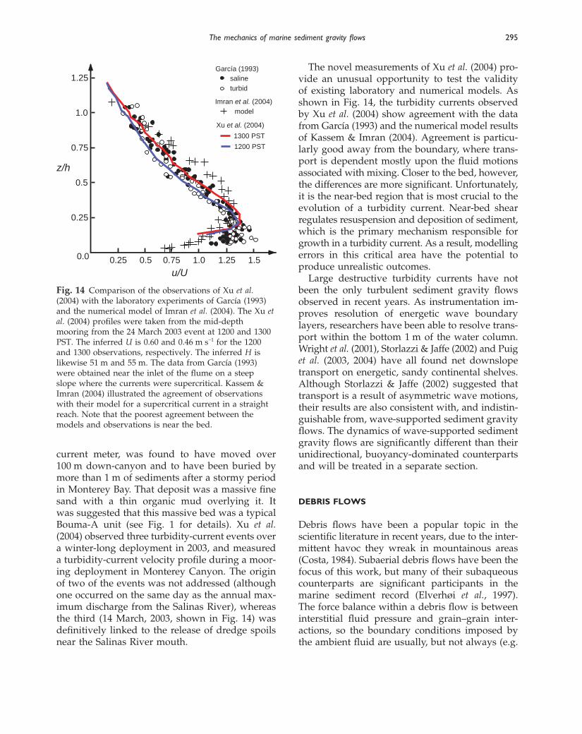
current meter, was found to have moved over 100 m down-canyon and to have been buried bymore than 1 m of sediments after a stormy periodin Monterey Bay. That deposit was a massive finesand with a thin organic mud overlying it. It was suggested that this massive bed was a typicalBouma-A unit (see Fig. 1 for details). Xu et al.(2004) observed three turbidity-current events overa winter-long deployment in 2003, and measureda turbidity-current velocity profile during a moor-ing deployment in Monterey Canyon. The originof two of the events was not addressed (althoughone occurred on the same day as the annual max-imum discharge from the Salinas River), whereasthe third (14 March, 2003, shown in Fig. 14) wasdefinitively linked to the release of dredge spoilsnear the Salinas River mouth.
The novel measurements of Xu et al. (2004) pro-vide an unusual opportunity to test the validity of existing laboratory and numerical models. Asshown in Fig. 14, the turbidity currents observedby Xu et al. (2004) show agreement with the datafrom García (1993) and the numerical model resultsof Kassem & Imran (2004). Agreement is particu-larly good away from the boundary, where trans-port is dependent mostly upon the fluid motionsassociated with mixing. Closer to the bed, however,the differences are more significant. Unfortunately,it is the near-bed region that is most crucial to theevolution of a turbidity current. Near-bed shear regulates resuspension and deposition of sediment,which is the primary mechanism responsible forgrowth in a turbidity current. As a result, modellingerrors in this critical area have the potential toproduce unrealistic outcomes.
Large destructive turbidity currents have notbeen the only turbulent sediment gravity flowsobserved in recent years. As instrumentation im-proves resolution of energetic wave boundary layers, researchers have been able to resolve trans-port within the bottom 1 m of the water column.Wright et al. (2001), Storlazzi & Jaffe (2002) and Puiget al. (2003, 2004) have all found net downslopetransport on energetic, sandy continental shelves.Although Storlazzi & Jaffe (2002) suggested thattransport is a result of asymmetric wave motions,their results are also consistent with, and indistin-guishable from, wave-supported sediment gravityflows. The dynamics of wave-supported sedimentgravity flows are significantly different than theirunidirectional, buoyancy-dominated counterpartsand will be treated in a separate section.
DEBRIS FLOWS
Debris flows have been a popular topic in the scientific literature in recent years, due to the inter-mittent havoc they wreak in mountainous areas(Costa, 1984). Subaerial debris flows have been thefocus of this work, but many of their subaqueouscounterparts are significant participants in themarine sediment record (Elverhøi et al., 1997). The force balance within a debris flow is betweeninterstitial fluid pressure and grain–grain inter-actions, so the boundary conditions imposed by the ambient fluid are usually, but not always (e.g.
García (1993)
turbid
saline
modelImran et al. (2004)
Xu et al. (2004)
1300 PST
1200 PST
0.0 0.25 0.5 0.75 1.0 1.25 1.5
0.25
0.5
0.75
1.0
1.25
z/h
u/U
Fig. 14 Comparison of the observations of Xu et al.(2004) with the laboratory experiments of García (1993)and the numerical model of Imran et al. (2004). The Xu etal. (2004) profiles were taken from the mid-depthmooring from the 24 March 2003 event at 1200 and 1300PST. The inferred U is 0.60 and 0.46 m s−1 for the 1200and 1300 observations, respectively. The inferred H islikewise 51 m and 55 m. The data from García (1993)were obtained near the inlet of the flume on a steepslope where the currents were supercritical. Kassem &Imran (2004) illustrated the agreement of observationswith their model for a supercritical current in a straightreach. Note that the poorest agreement between themodels and observations is near the bed.
CMS_C06.qxd 4/27/07 9:18 AM Page 295

296 J.D. Parsons et al.
hydroplaning), of little consequence. As a result,many of the concepts formulated for subaerial flowscan be extended to the marine environment.
Central to any discussion of debris flows is thetopic of rheology. Rheology is the study of themovement of a material under an applied stress.It is highly dependent on the grain size and mineralogy of the constituent material, the watercontent of the sample, and a host of other geo-technical (lithological) parameters. A detailed de-scription of subaqueous-debris-flow and slide rheology has been presented in Lee et al. (this volume, pp. 213–274). In the present paper, recentadvances will be discussed in the resolution of the mechanics for fluids of arbitrary rheology (i.e. non-Newtonian fluids).
Basic mechanics
As mentioned in Lee et al. (this volume, pp. 213–274), rheology of debris flow material plays animportant role in the stability and mobility of theflow itself. Two models have emerged, which havedifferent underlying assumptions about the rela-tionship between stress and strain in debris flows.The first, oldest, and simplest is the Herschel–Bulkley model, which characterizes the relation-ship between the imposed stress τx and the strainrate ∂u/∂z through a power law. Mathematically,this relationship can be expressed as
τx − τ0 = Kn
(1)
for a two-dimensional flow in the x–z plane, withvelocity strictly in the x-direction. Here the yieldstrength τ0, K and n are all empirically derived and material specific. These parameters can havea large range of values, which are generally scaledependent (Parsons et al., 2001b). However, forthe largest flows (volumes in excess of 0.001 km3),they tend to approach a fixed value (Dade &Huppert, 1998).
A common simplification of the Herschel–Bulkleymodel is the Bingham-plastic model. A Bingham-plastic model occurs when n = 1 in Eq. 1. In thiscase, µ becomes equivalent to a dynamic viscosity(units: Pa · s = N · s m−2). The dynamic viscosity ofmost natural debris flows is > 100 Pa s (Whipple
KK
∂u∂z
HH
& Dunne, 1992), so Reynolds numbers of debrisflows are usually in the order of 1. As a result, tur-bulence is generally thought to be unimportant.Bingham materials, like paint, also have a tend-ency to ‘freeze’ once their thickness becomes lessthan that required to shear the material. That is, thecritical thickness
hcr = (2)
where ρ is the density of the debris flow material(usually ~2.2 kg m−3) and β is the bed slope. TheBingham model (viscoelasticity) is particularly relevant when hcr is a significant portion of the flow thickness. This is often the case when eitherthe material is clay-rich or when the flows beingstudied are small (Parsons et al., 2001b). Viscoelasticeffects are generally less important when the flowsbecome large and coarse-grained (Iverson, 1997; Leeet al., this volume, pp. 213–274).
A more sophisticated approach is to assume thatthere are two distinct phases present within a single flow. Dubbed mixture theory, the governingequations being solved are similar to those discussedwith regard to the shallow-water equations (see Box 1). For highly concentrated mixtures, com-plications arise as the density is not fixed, but is a function of the solids content within the flow. Thegoverning equations become increasingly complexwith the addition of the second phase, so analyticalsolutions are limited (Denlinger & Iverson, 2001).Even numerical solutions of mixture theory are com-putationally demanding, particularly when flow isover irregular (i.e. realistic) topography (Denlinger& Iverson, 2001, 2004).
Considering the potential importance of inter-granular friction in the dissipation of energy in largesubmarine debris flows, future modelling studiesare likely to use mixture theory. However, mixturetheory has never been adapted for the marineenvironment. Hydroplaning, which was discoveredduring the STRATAFORM programme and will be discussed next, presents unusual challenges nottypically encountered in subaerial applications. It is uncertain how to incorporate the mechanics of the ambient fluid (important for hydroplaning)into the formulation derived in Box 2. As a resultof this uncertainty and the general lack of coarse
τ0
ρg tan β
CMS_C06.qxd 4/27/07 9:18 AM Page 296

The mechanics of marine sediment gravity flows 297
Box 2 Mixture theory (Iverson, 1997; Iverson & Denlinger, 2001)
Beginning with the conservation of momentum and mass
ρ = −∇ · (Ts + Tf + T′) + ρS [momentum] (B2.1a)
∂ρ/∂t + ∇ · (ρP) = 0 [mass] (B2.1b)
Unlike in the single-phase shallow-water equation derivation (see Box 1), the density of the fluid ρ is not constant,but dependent on the mixture of the volume of solids (sediment) Vs and fluid Vf, such that
ρ = ρsVs + ρfVf (B2.2)
T′ is the stress tensor associated with the relative motion of the solid and fluid components with respect to the flowas a whole, so
T′ = −ρsVs(Ps − P)(Ps − P) − ρfVf(Pf − P)(Pf − P) (B2.3)
where the subscripts f and s denote fluid and solid phase, respectively. The relative stress T′ is assumed negligibleand the reference frame is taken with respect to the solid phase only, which simplifies Eqs B2.1 to
ρ = −∇ · (Ts + Tf ) + ρS [momentum] (B2.4a)
∇ · Ps = 0 [mass] (B2.4b)
Now assuming a rigid boundary and depth averaging the conservation equations (i.e. similar to Eq. B1.8), it is foundthat
+ + = 0 (B2.5a)
ρ + + = −�h
0
+ + + + + − ρdfgx dz (B2.5b)
where Ts(ij) and Tf(ij) are the ij component in the stress tensor for the solid and fluid phase, respectively. U and V arethe depth-averaged velocities in the x and y direction. Equation B2.5a is the (final) conservation of mass equationand Eq. B2.5b is the x-direction conservation of momentum. Note that the conservation of mass is identical to its shallow-water-equation equivalent (i.e. Eq. B1.8c). The y-direction conservation of momentum is obtained by inter-changing x with y and U with V.
Using Leibniz’ theorem to evaluate the solid stress portion of the right-hand side of Eq. B2.5b
−�h
0
+ + dz = + + τbx (B2.6)
where {s(ij) is the ijth component of the depth-averaged stress and τbx = Ts(zx)4z=0 is the bed shear stress in the x-direction.Again, the same equation holds for the y-direction when x and y are interchanged. The weight of the slurry is
{s(zz) + {f(zz) = ρgzh/2 (B2.7)
which can be related to the depth-averaged normal stresses (e.g. {s(xx)). Here, Iverson & Denlinger (2001) used a lateral stress coefficient kact/pass derived from Coulomb theory. By definition
{s(xx) + {s(yy) = kact/pass{s(zz) (B2.8)
The lateral stress coefficient takes a value of 1 if Coulomb failure does not occur within the material. However, theprimary case of interest is when failure occurs, such that it can be shown from Coulomb theory that
∂(h{s(yx))
∂y
∂(h{s(xx))
∂x
JL
∂Ts(zx)
∂z
∂Ts(yx)
∂y
∂Ts(xx)
∂x
GI
JL
∂Tf(zx)
∂z
∂Ts(zx)
∂z
∂Tf(yx)
∂y
∂Ts(yx)
∂y
∂Tf(xx)
∂x
∂Ts(xx)
∂x
GI
JL
∂ (UVh)
∂y
∂(U2h)
∂x
∂ (Uh)
∂t
GI
∂(Vh)
∂x
∂ (Uh)
∂x
∂h
∂t
DPs
Dt
DP
Dt
CMS_C06.qxd 4/27/07 9:18 AM Page 297

298 J.D. Parsons et al.
kact/pass = (B2.9)
where φint is the internal friction angle of the solid material composing the debris flow. Assuming that the fluid withinthe debris flow is hydrostatic ({s(zz) = pbed/2), and substituting this into Eqs B2.7 and B2.8, the depth-averaged com-ponents of the solid-phase stress tensor become
{s(xx) = {s(yy) = kact/pass[(ρgzh − pbed)/2] (B2.10)
The normal stresses are geometrically related to the tranverse shear stresses (via ‘Mohr’s circle’) in a Coloumb mix-ture, such that
{s(yx) = {s(xy) = −sgn(∂U/∂y){kact/pass[(ρgzh − pbed)/2]}sin φint (B2.11)
The bed shear stress τbx is similarly related to the normal stresses (i.e. through Mohr’s circle), through the frictionangle at the bed φbed · φbed > φint, if there is bed roughness. The resulting expression is
{s(zx) = −sgn(U)(ρgzh − pbed)tan φbed (B2.12)
The fluid stresses are more straightforward. Here the fluid stresses are expressed as they are on the right-hand sideof Eq. B1.3
−�h
0
+ + dz = −�h
0
− Vfµ + + dz (B2.13)
where µ is the dynamic viscosity of interstitial fluid. The first term on the right-hand side is the product of the pressure gradient at the bed and the flow depth h, owing to the hydrostatic approximation. Integration of the nexttwo terms requires an application of Leibniz’ theorem, which simplifies to the simple product of the existing termswhen a ‘slab approximation’ (∂h/∂x = 0) is made. A slab approximation is implicit in the application of the Coulombequations to the problem at hand. Finally, the application of a no-slip boundary and an assumption of a parabolicvertical velocity profile yields the last term, such that
−�h
0
+ + dz = −h + Vfµh + Vfµh − 3Vfµ (B2.14)
Combining Eqs B2.10–B2.12 and B2.14 results in the final x-direction conservation of momentum equation
ρ + + = −sgn(U)(ρgzh − pbed)tan φbed − 3Vfµ (B2.15)
a b
−hkact/pass (ρgzh − pbed) − h + Vfµh
c
−sgn hkact/pass (ρgzh − pbed)sin φint + Vfµh + ρgxh
d e
Equation B2.5a combined with Eq. B2.15 and its y-direction complement (interchanging x and U with y and V) arethe final governing equations. Term a is the material derivative describing debris-flow motion, b is the bed shearstress, c is the streamwise normal stress, d is the transverse stress and e is the driving (gravity induced) stress. For adetailed description of the conservation of mass equation (B2.5a), see Box 1. For more details regarding the assump-tions made in the derivation above, consult the primary work of Iverson & Denlinger (2001).
! @
∂ 2U
∂y2
∂∂y
DF
∂U
∂y
AC
1 4 4 4 4 4 4 4 2 4 4 4 4 4 4 4 3
∂ 2u
∂x 2
∂pbed
∂x
∂∂x
1 4 4 4 4 4 2 4 4 4 4 4 31 4 4 4 4 2 4 4 4 4 3
U
h
JL
∂(UVh)
∂y
∂(U2h)
∂x
∂(Uh)
∂t
GI
U
h
∂ 2U
∂y2
∂ 2U
∂x2
∂pbed
∂x
JL
∂Tf(zx)
∂z
∂Tf(yx)
∂y
∂Tf(xx)
∂x
GI
JL
DF
∂ 2U
∂z2
∂ 2U
∂y2
∂ 2U
∂x2
AC
∂p
∂x
GI
JL
∂Tf(zx)
∂z
∂Tf(yx)
∂y
∂Tf(xx)
∂x
GI
1 + sin2 φint
1 − sin2 φint1 4 4 4 4 4 4 4 4 4 2 4 4 4 4 4 4 4 4 3
CMS_C06.qxd 4/27/07 9:18 AM Page 298

The mechanics of marine sediment gravity flows 299
material in the deep-sea environment, all of the analysis performed to date on submarine debrisflows has assumed a Bingham or Herschel–Bulkleyrheology.
Hydroplaning
Although submarine debris flows share manysimilarities with their better-studied subaerialcounterparts, they differ in striking ways. Recentlaboratory comparisons of subaqueous and sub-aerial debris flows and their products have not onlyhighlighted these differences, but have providedphysical explanations for the differences as well(Mohrig et al., 1998, 1999; Marr et al., 2001; Tonioloet al., 2004). The physical insight gained in thesestudies is guiding the development of numericalmodels for submarine debris flows (Harbitz et al.,2003). The knowledge also aids the interpretationof ancient debris-flow deposits. Since most of theavailable data on submarine debris flows consistof geometric and compositional information fromtheir deposits, advancing inversion methods areessential. Inverse models and the informationgleaned from them are particularly useful in con-straining runout and emplacement processes.
Laboratory experiments have documented thesignificant role of ambient-fluid density on the beha-viour of subaqueous and subaerial debris flows.Water is about 800 times more dense than air, sothe inertial forces associated with a debris flow, accelerating fluid out of its path as it moves down-slope produce substantially larger dynamic pressuresat the front of a subaqueous flow (as compared witha subaerial debris flow). Accentuating this effect is the relatively small difference (by about a factorof two) between the density of the ambient fluid(water) and the debris-flow slurry. When pressuresdevelop that are comparable in magnitude to thesubmerged weight per unit bed area of the flow, it can no longer displace water from its contact area with the bed fast enough and a layer of fluid begins to separate the debris from the bed.Mohrig et al. (1998) proposed that the instigationof dynamic hydroplaning is suitably character-ized by a densimetric Froude number Frd = Uf/
, where Uf is the head velocity of the flowor slide, g′ is the reduced gravitational acceleration(i.e. (ρ1 − ρ0)g/ρ0, with g the gravitation accelera-tion, ρ1 the density of the debris flow and ρ0 the
g′h cos β
ambient density), h is the average thickness of the flow or slide and β denotes the slope of the bed. The densimetric Froude number describesthe balance between hydrodynamic pressure andthe submerged debris load. It has been used withgreat success in scaling the effects of the resultantpressure force on a moving body (Brown, 1975).Laboratory flows constrain hydroplaning to caseswhere Frd is greater than 0.4, a value that is con-sistent with fast moving, natural debris flows(Mohrig et al., 1998).
The initial laboratory experiments that deter-mined the conditions for and the consequences of hydroplaning were all conducted in the ‘FishTank’, a glass-walled tank 10 m long, 3 m high and 1 m wide in the St Anthony Falls Laboratory.Suspended within the Fish Tank is a 0.2-m widechannel, sufficiently narrow to ensure conditionsfor two-dimensional flow. The tank was filled withwater or drained for subaqueous and subaerialruns, respectively. The front velocities for most of the observed subaqueous debris flows weregreater than their subaerial counterparts. The sub-aqueous runout distances were also larger (Mohrig et al., 1998, 1999). Direct observation revealed thatthe thin layer of water that penetrated beneath the front of the hydroplaning debris flow acted as a lubricant (Figs 15A & B & 16). These easilysheared lubricating layers of water dramaticallyreduced the bed resistance acting on the debris,thereby increasing their relative mobility. Averagethicknesses for the lubricating layers were small and in all cases < 2% of the thickness of the over-riding debris flow or slide.
The thickness of a lubricating water layer beneatha hydroplaning debris flow was always observedto decrease with distance from the flow front. Thisspatial change in layer thickness caused a differ-ence in forward velocity between the debris ridingon a discrete layer of water and the trailing portionof the flow that was more attached to the bed. Theresult was a stretching and attenuation of the flowdirectly behind its front. In some runs, the headautoacephalates (i.e. separates from the body),causing a new head to form. The detached blocksslid to the end of the channel in front of the newlyformed head of the flow. These isolated outrunnerblocks (Figs 17 & 18) are commonly observedassociated with the deposits of submarine debrisflows (Prior et al., 1984; Lipman et al., 1988; Nissen
CMS_C06.qxd 4/27/07 9:18 AM Page 299
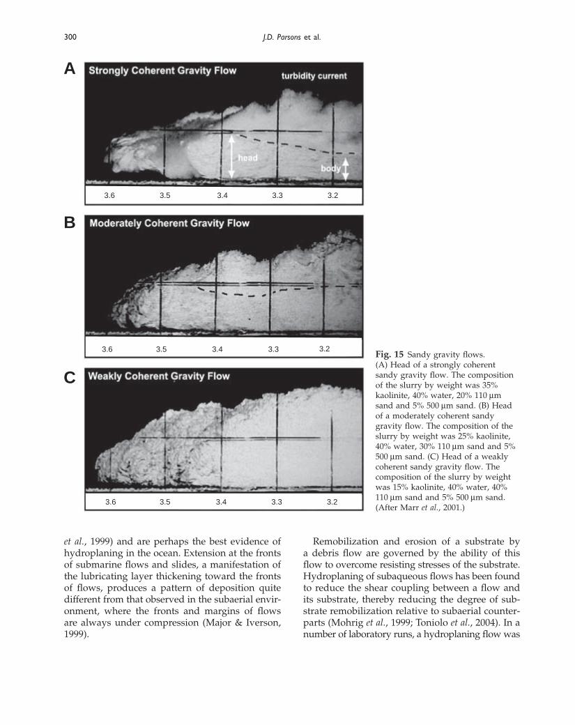
300 J.D. Parsons et al.
et al., 1999) and are perhaps the best evidence ofhydroplaning in the ocean. Extension at the frontsof submarine flows and slides, a manifestation ofthe lubricating layer thickening toward the frontsof flows, produces a pattern of deposition quite different from that observed in the subaerial envir-onment, where the fronts and margins of flows are always under compression (Major & Iverson,1999).
Remobilization and erosion of a substrate by a debris flow are governed by the ability of this flow to overcome resisting stresses of the substrate.Hydroplaning of subaqueous flows has been foundto reduce the shear coupling between a flow andits substrate, thereby reducing the degree of sub-strate remobilization relative to subaerial counter-parts (Mohrig et al., 1999; Toniolo et al., 2004). In anumber of laboratory runs, a hydroplaning flow was
A
B
C
3.6 3.5 3.4 3.3 3.2
3.6 3.5 3.4 3.3 3.2
3.6 3.5 3.4 3.3 3.2
Fig. 15 Sandy gravity flows. (A) Head of a strongly coherentsandy gravity flow. The compositionof the slurry by weight was 35%kaolinite, 40% water, 20% 110 µmsand and 5% 500 µm sand. (B) Headof a moderately coherent sandygravity flow. The composition of theslurry by weight was 25% kaolinite,40% water, 30% 110 µm sand and 5%500 µm sand. (C) Head of a weaklycoherent sandy gravity flow. Thecomposition of the slurry by weightwas 15% kaolinite, 40% water, 40%110 µm sand and 5% 500 µm sand.(After Marr et al., 2001.)
CMS_C06.qxd 4/27/07 9:18 AM Page 300

The mechanics of marine sediment gravity flows 301
found to have moved over a very soft substratewithout reactivating any measurable amount of therecent deposit. The role of a thin lubricating layeron reducing the transmission of shear stress froman overriding flow into the bed was quantitativelydeveloped by Harbitz et al. (2003).
Further experiments on subaqueous debris flowsin the Fish Tank have focused on the role of claycontent on the dynamics and deposition of sub-aqueous debris flows (Marr et al., 2001). Studieswere performed using pre-mixed slurries contain-ing 110 µm sand, clay and water. The experimentsindicated that as little as 0.7–5% by weight of bentonite clay or 7–25% by weight of kaolinite clayat water contents ranging from 25 to 40% by weightwas required to generate coherent gravity flows
Fig. 17 A glide blockautoacephalated from the body of asubaqueous debris flow. (A) Viewlooking upstream of a subaqueousdebris-flow deposit that passed overan antecedent deposit. Most of thematerial did not participate inhydroplaning; however, a small mass(an outrunner block) hydroplanednear the front. The path of theoutrunner block can be seen in theglide track just downstream of themain flow mass. (B) Plan view of theglide block that autoacephalated andhydroplaned off the main platform(just below the view of camera in A).
with a substantial basal debris-flow component. At lower clay contents, the flows were transitionalto highly concentrated turbidity currents. Increasedwater content also favoured the formation of tur-bidity currents.
Examination of the boundary between debrisflows and turbidity currents is important for identifying and interpreting sediment gravity-flowdeposits, but also for the creation of a turbidity current from failed material. Transition from debrisflows to turbidity currents is discussed at length in
A B
outrunner block
piece ofblock
primary debris-flowdeposit
glide track
glide trackGlide block!!Glide block!!
1 km
glide block
Fig. 16 Hydroplaning head of an unconfinedsubaqueous debris flow. The photograph was taken froman underwater video camera looking upstream.
Fig. 18 Multibeam bathymetric image of the depositsfrom two submarine flows in a Norwegian fjord. Thedeposits were caused by an adjacent subaerial landslidethat flowed into the fjord in 1996. A single glide block(black arrow) hydroplaned to the opposite side of thefjord (path of white arrow). (Image appears courtesy ofAnders Elverhøi.)
CMS_C06.qxd 4/27/07 9:18 AM Page 301
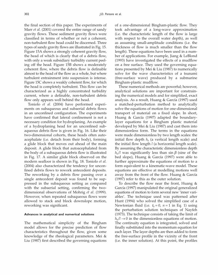
302 J.D. Parsons et al.
the final section of this paper. The experiments ofMarr et al. (2001) covered the entire range of sandygravity flows. These sediment gravity flows wereclassified in terms of whether or not a coherent, non-turbulent flow head could be discerned. Threetypes of sandy gravity flows are illustrated in Fig. 15.Figure 15A shows a strongly coherent gravity flow,the head of which is clearly that of a debris flow,with only a weak subsidiary turbidity current peel-ing off the head. Figure 15B shows a moderatelycoherent flow, where the debris flow is definablealmost to the head of the flow as a whole, but whereturbulent entrainment into suspension is intense.Figure 15C shows a weakly coherent flow, for whichthe head is completely turbulent. This flow can becharacterized as a highly concentrated turbidity current, where a definable, non-turbulent debrisflow only appears well behind the head.
Toniolo et al. (2004) have performed experi-ments on subaqueous and subaerial debris flowsin an unconfined configuration. The experimentshave confirmed that lateral confinement is not a necessary condition for hydroplaning. An exampleof a hydroplaning head for an unconfined sub-aqueous debris flow is given in Fig. 16. Like theirtwo-dimensional cohorts, these heads often auto-acephalate (i.e. detach from their body), forming a glide block that moves out ahead of the maindeposit. A glide block that autoacephalated fromthe body of a subaqueous debris flow is illustratedin Fig. 17. A similar glide block observed on themodern seafloor is shown in Fig. 18. Toniolo et al.(2004) also characterized the tendency for uncon-fined debris flows to rework antecedent deposits.The reworking by a debris flow passing over a single antecedent deposit was found to be sup-pressed in the subaqueous setting as compared with the subaerial setting, confirming the two-dimensional observations of Mohrig et al. (1999).However, when repeated subaqueous flows wereallowed to stack and block downslope motion,reworking was significant.
Advances in analytical and numerical solutions
The mathematical simplicity of the Binghammodel allows for the precise prediction of flow characteristics throughout the flow, given someknowledge of the rheological parameters. Mei & Liu (1987) first described the governing equations
of a one-dimensional Bingham-plastic flow. Theytook advantage of a long-wave approximation(i.e. the characteristic length of the flow is large with respect to the overall water depth), as well as assuming small-amplitude conditions (i.e. thethickness of flow is much smaller than the flowlength). These equations have been used in a num-ber of applications. For example, Jiang & LeBlond(1993) have investigated the effects of a mudflowon a free surface. They used the governing equa-tions presented by Mei & Liu (1987) to numericallysolve for the wave characteristics of a tsunami(free-surface wave) produced by a submarineBingham-plastic mudflow.
These numerical methods are powerful; however,analytical solutions are important for constrain-ing the numerical models and for simplified, exactanalysis. As a result, Huang & García (1997) useda matched-perturbation method to analyticallysolve the equations of motion for one-dimensionaltransport of material on a fixed slope. In short,Huang & García (1997) adapted the boundary-layer equations for a Bingham plastic materialdeveloped by Mei & Liu (1987) and cast them intodimensionless form. The terms in the equationswere made dimensionless by two length scales: theinitial flow depth h0 (a vertical length scale) and the initial flow length l (a horizontal length scale).By assuming the characteristic dimensionless depthh0/l was significantly less than sin β (sine of the bed slope), Huang & García (1997) were able to further approximate the equations of motion to aform equivalent to a kinematic-wave model. Theseequations are effective at modelling motions wellaway from the front of the flow. Huang & García(1997) refer to this as the outer solution.
To describe the flow near the front, Huang &García (1997) manipulated the original generalizedequations of motion to form several new ‘inner vari-ables’. The technique used was patterned afterHunt (1994) who solved the simplified case of aNewtonian fluid (i.e. τ0 = 0, n = 1 in Eq. 1) using the perturbation solution techniques of Nayfeh(1973). The technique consists of taking the limit ofh0/l → 0 in the dimensionless equations of motion.The continuity equation is integrated, solved andfinally substituted into the momentum equation foreach layer. The layer depths are then added to formthe free-surface profile in the vicinity of the front(i.e. the inner solution). At this point, the profiles
CMS_C06.qxd 4/27/07 9:18 AM Page 302

The mechanics of marine sediment gravity flows 303
near the front and the outer solution are redimen-sionalized. Doing so, Huang & García (1997) foundthat the characteristic length scales l and h0 dropout, leaving a solution entirely of known variables.The result is shown in Fig. 19 as the composite solution. It is asymptotically accurate both near thefront and along the body. After a number of tests,Huang & García (1997) found that the solution isgenerally acceptable after the flow runs out threetimes the initial height.
Huang & García (1998) extended the results ofHuang & García (1997) for the more general case ofa Herschel–Bulkley fluid (Eq. 1). Due to the addi-tion of another variable (the exponent, n in Eq. 1),the analysis becomes increasingly complicated.Despite the complications, Huang & García (1998)were able to find a solution in a similar manner,thus forming a composite solution capable of char-acterizing the complex behaviour associated withthe more generalized rheological model.
Imran et al. (2001a,b) have extended the ana-lytical model of Huang & García (1998) to form‘BING’, a one-dimensional integral numerical modelof Herschel–Bulkley subaerial and subaqueousmuddy debris flows. The bilinear case does not havea closed-form asymptotic solution. Pratson et al.(2001) have used it and a shallow-water-equation
model for turbidity currents, ‘BANG’, to comparethe stacked deposits of turbidity currents and sub-marine debris flows. Hydroplaning is not yet in-corporated in BING. Criteria have been developedby Huang & García (1999) to assess the point atwhich hydroplaning will occur in standard one-dimensional Herschel–Bulkley flows. Resolutionof the mechanics once the flow begins to hydro-plane requires additional theory, however. In thisvein, Harbitz et al. (2003) have modified lubricationtheory to describe the equilibrium hydroplaning ofa thin block over a sloping bed. Their theoreticalformulation provides insight into the dynamics ofautoacephalated glide blocks.
Another challenge remaining is to extend thenumerical models of debris flows into two dimen-sions. It may seem that numerical models of realistic, two-dimensional debris flows should beattainable, particularly considering the analyticalsolutions available in the one-dimensional case (andthe success of two-dimensional turbidity-currentmodels). However, numerical models of higher-dimensional debris flows have proved to be particu-larly difficult. Unlike the one-dimensional modelsdiscussed above, matching analytical solutions are not easily available for the higher-dimensionalcase. Further, most finite-difference schemes are particularly sensitive to the moving boundary atthe debris-flow front. As a result, researchers areforced to solve the moving-boundary problem witha finite-element approach, similar to that taken byChoi & García (2001) for turbidity currents. Workproceeds to capture the dynamics of debris flowsin realistic geometries, but results have yet to befully tested.
Observations of submarine debris flows
In the search for oil, the petroleum companies andthe corporations that service their data-acquisitionneeds have imaged large portions of the seafloor.These new data have illustrated that submarine-debris-flow deposits are relatively common geo-logical features. Figure 20 provides an interestingcontrast between debris-flow deposits on twovery different continental margins, both of whichare actively being explored for petroleum. Theseexamples depict the dichotomy in debris-flow pro-cesses that is embodied in the two different rheo-logical models discussed in this paper.
0.3
0.2
0.1
00 5 10
initialcondition
Krone &Wright (1987) outer solution
compositesolution
h (m
)
x (m)
t = 4.1 s
Fig. 19 Comparison of the matched-asymptotic solutionof Huang & García (1997) with the experimental resultsof Krone & Wright (1987). Experimental conditions (other than those shown) are sin β = 0.06, τy = 42.5 Pa, µ = 0.22 Pa-s, ρ = 1073 kg m−3. The slight discrepancybetween the height of the flow in the experiment and inthe theory is most likely a result of the loss of materialdue to coating of the sidewalls in the flume.
CMS_C06.qxd 4/27/07 9:18 AM Page 303

304 J.D. Parsons et al.
Figure 20A & B illustrates two seismic cross-sections of an erosive, blocky debris flow com-prised primarily of fractured carbonate on theNova Scotian margin. The flow that produced thedeposit travelled over 10 km down a relativelyuniform slope of 9°. As can be seen in the image,the flow was extremely erosive, embedding itselfin the underlying stratigraphy. Similar seabedploughing has been observed in other large sub-marine debris flows (Prior et al., 1984). Large blocksthat appear to retain the stratigraphy of their source
are also common, and have been previously docu-mented in large, carbonate debris-flow deposits(Hine et al., 1992). Finally, the structure of theseabed surrounding the deposit is disturbed, evenbeyond the point at which the flow stopped. All ofthese characteristics suggest significant interactionwith the bed and substantial energy loss associ-ated with frictional contacts. To properly predictdebris-flow runout in this type of setting wouldrequire mixture theory (see Box 2). However, it is important to mention that even mixture theory
B
100 m 2 km
A1 km
100 m
deposit length (~9 km)
large blocks
deposit width (~10.4 km)
large block
dip lineconvolutedbedding
strike line
convolutedbedding
2 km
glide track
debris flow
pressureridges
outrunnerblock A
outrunnerblock B
C
Fig. 20 Contrast of different types of submarine debris flows. (A) Interpreted seismic (dip) cross-section of a blockysubmarine debris-flow deposit from the Nova Scotian continental margin. The blue area corresponds to the debris-flowdeposit, while orange corresponds to a region of deformed bedding found around the primary deposit. Regionsassociated with the debris-flow deposit (composed of ancient lithified carbonate-reef fragments) and deformed bedding(siliciclastic mud) were confirmed from several cores. (B) Interpreted strike cross-section from the same Nova Scotiadebris flow. (Data appear courtesy of L.G. Kessler.) (C) Depositional signature of a fine-grained, subaqueous debris flow.The image is a ‘time’ slice obtained from three-dimensional seismic tomography of the Nigerian margin (Nissen et al.,1999). The streaks seen in the figure are qualitatively identical to the smear that connects the outrunner block to itsparent in Fig. 17.
CMS_C06.qxd 4/27/07 9:18 AM Page 304

The mechanics of marine sediment gravity flows 305
does not include processes likely present in theNova Scotian case (e.g. fluidization from seismicand acoustic waves; Melosh, 1979).
Figure 20C is a ‘time slice’ from a seismic cubeacquired from the West African margin (Nissen et al., 1999). A time slice represents a single reflectorin the seismic cube, so it essentially yields a mapof an ancient seafloor. Highlighted in green are glidetracks from outrunner blocks circled in red. Thesefeatures bear an uncanny resemblance to the glidetracks and outrunner blocks seen in Fig. 18. Alsopresent are ‘pressure ridges’ commonly found inlaboratory experiments of Bingham-like materials(Major & Pierson, 1992; Parsons et al., 2001b). Onthe muddy, siliciclastic margin of West Africa, a single-phase fluid model (e.g. in Huang & García(1997) and the Fish Tank experiments) appears toencapsulate the most important physical processes.
WAVE-SUPPORTED SEDIMENT GRAVITY FLOWS
Wave-supported sediment gravity flows and estu-arine fluid muds, unlike debris flows and turbid-ity currents, have been studied primarily in thenatural environment. They result from a balancebetween wave, tidal and gravity-driven motions.Unlike the traditional conceptions of a sedimentgravity flow, they require some additional energysource (waves, tides or currents) to maintain their integrity. Due to difficulties associated withsampling the large fluxes of sediment close to thebed, progress in understanding their dynamics on continental shelves has come largely fromrecent multi-investigator studies (e.g. AmasSeds,STRATAFORM). These analyses are discussed be-low, along with the presentation of a model that iscapable of predicting transport based upon basicsedimentological variables (e.g. wave orbital velo-city Uw, critical bed shear stress τcr).
Estuarine fluid muds have been found in manycoastal settings where sediment supply exceedstransport capacity (Wells, 1983; Wright et al., 1990;Kineke et al., 1996). However, conditions are notamenable to the formation of estuarine fluid mudson the shelf near the Eel River. Much of theknowledge about the mechanics of estuarine fluidmuds stems from the work done on the Amazonshelf (Kineke & Sternberg, 1992, 1995; Trowbridge& Kineke, 1994; Cacchione et al., 1995; Kineke et al.,
1996). In particular, Trowbridge & Kineke (1994) setforth a simple model of an impulsively generated,periodic boundary layer, which can be applied toall boundary layers dominated by fine sediment,and will be used below to describe wave-supportedsediment gravity flows. Work in other locales hasdocumented that tidally derived fluid muds arecommon and important for the cross-shelf trans-port of sediment, as well as the construction of shelfclinoforms in many settings (e.g. Fly River margin,Papua New Guinea; Walsh et al., 2004).
Unlike estuarine fluid muds, wave-supportedsediment gravity flows were commonly observedon the northern California margin. As discussed in Hill et al. (this volume, pp. 49–99), high con-centrations of wave-suspended sediment isolatednear the bed are an important cause for downslopetransport on the Eel shelf during and after floodevents (Fig. 21). Wave-supported sediment gravityflows are also important for creating mid-shelfflood deposits. These flows are fundamentally dif-ferent from other gravity flows discussed in thispaper, because the turbulent energy required to keepthe sediment in suspension is supplied primarilyby surface waves and not by the flow itself. Thiswas seen in the observations made at a 60-m Eelshelf site (K60) during January 1998 (Fig. 21). Thethickness of the highly concentrated near-bedlayer is roughly equivalent to the wave-boundary-layer height predicted by
δw = (3)
where the wave friction factor fw is described by Swart (1974), ω is the radial frequency and Uw is the root-mean-square wave orbital velocity(Traykovski et al., 2000). Further support for the role of waves comes from the correlation of wavecessation with the collapse of the gravity-flowlutocline (i.e. turbidity discontinuity). As will beshown below, similar behaviour has been seen in laboratory experiments.
Wave-boundary-layer mechanics
The internal mechanics within wave boundarylayers, due to their fluid-mechanical complexity(highly sheared, unsteady flows confined within
fw
δUw
ω
CMS_C06.qxd 4/27/07 9:18 AM Page 305
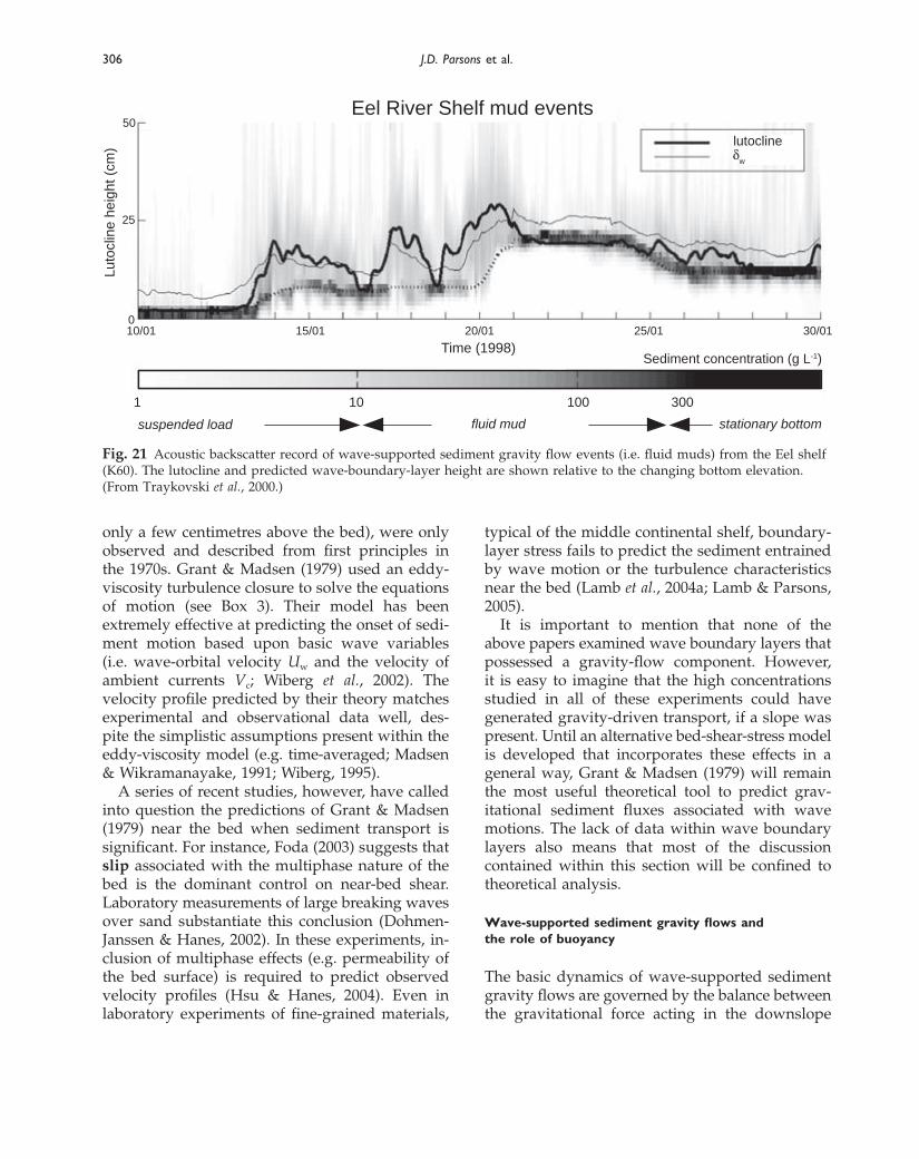
306 J.D. Parsons et al.
only a few centimetres above the bed), were onlyobserved and described from first principles inthe 1970s. Grant & Madsen (1979) used an eddy-viscosity turbulence closure to solve the equationsof motion (see Box 3). Their model has beenextremely effective at predicting the onset of sedi-ment motion based upon basic wave variables (i.e. wave-orbital velocity Uw and the velocity ofambient currents Vc; Wiberg et al., 2002). Thevelocity profile predicted by their theory matchesexperimental and observational data well, des-pite the simplistic assumptions present within theeddy-viscosity model (e.g. time-averaged; Madsen& Wikramanayake, 1991; Wiberg, 1995).
A series of recent studies, however, have calledinto question the predictions of Grant & Madsen(1979) near the bed when sediment transport issignificant. For instance, Foda (2003) suggests thatslip associated with the multiphase nature of thebed is the dominant control on near-bed shear.Laboratory measurements of large breaking wavesover sand substantiate this conclusion (Dohmen-Janssen & Hanes, 2002). In these experiments, in-clusion of multiphase effects (e.g. permeability ofthe bed surface) is required to predict observedvelocity profiles (Hsu & Hanes, 2004). Even in laboratory experiments of fine-grained materials,
typical of the middle continental shelf, boundary-layer stress fails to predict the sediment entrainedby wave motion or the turbulence characteristicsnear the bed (Lamb et al., 2004a; Lamb & Parsons,2005).
It is important to mention that none of theabove papers examined wave boundary layers thatpossessed a gravity-flow component. However, it is easy to imagine that the high concentrationsstudied in all of these experiments could havegenerated gravity-driven transport, if a slope waspresent. Until an alternative bed-shear-stress modelis developed that incorporates these effects in a general way, Grant & Madsen (1979) will remainthe most useful theoretical tool to predict grav-itational sediment fluxes associated with wavemotions. The lack of data within wave boundarylayers also means that most of the discussion contained within this section will be confined to theoretical analysis.
Wave-supported sediment gravity flows and the role of buoyancy
The basic dynamics of wave-supported sedimentgravity flows are governed by the balance betweenthe gravitational force acting in the downslope
Eel River Shelf mud events
lutoclineδ
w
Luto
clin
e he
ight
(cm
)50
25
010/01 15/01 20/01 25/01 30/01
Time (1998)Sediment concentration (g L-1)
fluid mud stationary bottomsuspended load
1 10 100 300
Fig. 21 Acoustic backscatter record of wave-supported sediment gravity flow events (i.e. fluid muds) from the Eel shelf(K60). The lutocline and predicted wave-boundary-layer height are shown relative to the changing bottom elevation.(From Traykovski et al., 2000.)
CMS_C06.qxd 4/27/07 9:18 AM Page 306

Box 3 Shear stress and velocity distribution within wave boundary layers (Grant & Madsen, 1979)
Once again beginning with the incompressible, irrotational Navier–Stokes equations, which describe the conserva-tion of mass and momentum over an arbitrary control volume
= + ν∇2P (B3.1)
Defining an eddy viscosity K
K = κ4u*cw4z (B3.2)
where 4u*cw 4 is the total shear stress both from wave and currents, κ is the von Karman constant. Also defining thewave motions at the outer edge of the wave boundary layer
P∞ = 4Tw 4exp(iωt) (B3.3)
where i = −1, Tw is the near-bed wave orbital velocity (outside the wave boundary layer) and ω is the wave frequency. Assuming that the convective acceleration terms are encapsulated within the eddy-viscosity model K andthe background current is much smaller, Eq. B3.1 becomes
= − + κ4P*cw4z (B3.4)
If vertical velocities near the bed are assumed negligible, the y-direction of Eq. B3.4 yields
= − (B3.5)
Substituting Eq. B3.5 into Eq. B3.4 and defining (uw − u∞) = w0 = 4w0 4exp(iωt) yields
z − i4w04= 0 (B3.6)
Making the change of variables, Eq. B3.6 becomes
ζ − i34w04= 0 (B3.7)
Applying the boundary conditions,
near bed ⇒ w0 → −u∞ at ζ0 = kbω/30κ4u*cw4at the top of the boundary layer ⇒ w0 → 0 as ζ → ∞,
the general solution of Eq. B3.7 given these boundary conditions is
w0 = A1(Ber 2 ζ + i Bei 2 ζ ) + A2(Ker 2 ζ + i Kei 2 ζ ) (B3.8)
where Ber, Bei, Ker and Kei are Kelvin functions of zeroth order. A1 = 0 because Ber and Bei become large for ζ → ∞,which allows for the solution of the second integration constant
A2 = (B3.9)(Ker 2 ζ + i Kei 2 ζ )
Substituting Eq. B3.9 into Eq. B3.8 and exchanging variables yields the velocity profile
uw = 1 − u∞ (B3.10)Ker 2 ζ 0 + i Kei 2 ζ 0
DF
AC
−u∞
DF
∂4w0 4∂ζ
AC
∂∂ζ
DF
∂Pw
∂z
κ 4P*cw 4ω
AC
∂∂z
∇pw
ρ∂P∞
∂t
DF
∂Pw
∂z
AC
∂∂z
∇pw
ρ∂Pw
∂t
∇p
ρDP
Dt
Ker 2 ζ + i Kei 2 ζ
CMS_C06.qxd 4/27/07 9:18 AM Page 307

308 J.D. Parsons et al.
direction and the vertical distribution of shear stressin the water column
g′ sin β = dτ/dz (4)
where g′ is the reduced gravitational accelerationwith respect to the ambient water column, τ is theshear stress and z is the direction perpendicular tothe bed. The value of g′ is given by (ρ1 − ρ0)g/ρ0,where g is the gravitation acceleration, ρ1 is the density within the gravity flow and ρ0 is the ambi-ent seawater density. For sediment-driven flows, g′ = RCg, where C is the volumetric sediment con-centration and R = (ρsed − ρ0)/ρ0 is the submergedweight of the sediment in water. Integration of Eq. 4 over the wave-boundary-layer thickness yieldsthe familiar Chezy balance between frictional dragon the stationary seafloor τb, interfacial drag τi
from the water above and the gravitational force
(τb + τi)/ρa = B sin β (5)
where B is the depth-integrated reduced gravita-tional acceleration or ‘buoyancy’, given by
B = gR�0
δ w
Cdz (6)
Other terms such as Coriolis acceleration, largerscale pressure gradients and fluid accelerations aregenerally found or assumed to be small and there-fore can be neglected (Traykovski et al., 2000).
Determination of the buoyancy B and the dis-tribution of shear in the water column dτ/dz interms of measurable sedimentological properties(e.g. wave-orbital velocity, settling velocity) is central to any wave-supported sediment gravityflow model. As part of the STRATAFORM pro-gramme, several different approaches to model-ling these quantities have been investigated. To calculate the buoyancy B, two different analyseshave been used. The first assumes that the waveboundary layer is in equilibrium and well mixed.The result is an approximation akin to the Exnerapproximation used in classic sediment-transporttheory. However, in wave-supported sedimentgravity flows, the large values of sediment con-centration strongly stratify the water column andsuppress turbulence. Therefore, an alternative ap-proach to modelling the buoyancy has been devel-
oped to determine the maximum suspended loadpossible without suppressing the turbulence belowthat level.
Regardless of approach, relation of the sedi-ment in suspension to commonly measured wavevariables requires a model for the near-bed sedi-ment concentration. The near-bed sediment con-centration can often be calculated by equating theupward and downward flux of sediment. Here, thebalance will be considered as it applies to gravityflows trapped near the bed. Assuming that thedownward flux of sediment occurs through ballisticsettling with a settling velocity ws, the volumetricdepositional flux D = Cbws, where Cb is the near-bedvolumetric concentration and ws is the settlingvelocity of the sediment. Upward sediment fluxfrom the seabed is parameterized by an entrainmentrate E = Ews, where E is the dimensionless entrain-ment rate. From early studies, it was noted that thedimensionless entrainment rate could be altern-atively thought of as a concentration. As a result,E is sometimes called the reference concentrationrequired for sediment resuspension (Smith &McLean, 1977; Harris & Wiberg, 2001).
Description of the dimensionless entrainmentrate in terms of water-column properties has beenthe focus of innumerable studies over the past 30 yr. Two of these models have emerged as themost popular. García & Parker (1991, 1993), dis-cussed at length in the section on turbidity currents,is most often used by numerical modellers becauseit prescribes, for all entrainment rates, the distanceabove the bed at which E is to be observed (i.e. 5%of the total flow depth). The model of Smith &McLean (1977), on the other hand, is constructedsuch that the distance above the bed correspond-ing to E is also an empirical function. Prescriptionof the reference height (i.e. the height at which E is obtained) and the dimensionless entrainmentrate makes numerical modelling on fixed gridsdifficult, but it allows for greater flexibility in theformation of the model. It is also well tailored to temporal observations made at a fixed distanceabove the bed. As a result, the Smith & McLean(1977) formulation has been used primarily to calculate entrainment fluxes from field data, whereparticle size and behaviour (i.e. flocculated versusunflocculated) may differ significantly from thenon-cohesive, sandy flows explored by García &Parker (1991). The Smith & McLean (1977) model
CMS_C06.qxd 4/27/07 9:18 AM Page 308

The mechanics of marine sediment gravity flows 309
has been tested extensively with tripod measure-ments on many margins (including the Eel) withfine-sand and silty beds (Cacchione et al., 1999;Harris & Wiberg, 2001). The model has the generalform
E = (7)
where Ss = (τb − τcr)/τcr is the excess shear stress, τb is the bed shear stress, τcr is the critical shear stress to initiate motion, n is the porosity of the bed and γ0 is an empirical constant. It also requiresa formulation for the reference height. However, it will be shown that the reference height is not a relevant parameter in the calculation of the near-bed buoyancy.
To calculate the concentration distribution in thewave boundary layer, the upward flux of sedimentabove the reference height must also be known. The flux of sediment due to turbulent diffusion isusually thought to scale with the shear velocity, u*. If these quantities are assumed to be directlyrelated, the ratio of ws/u* determines the shape ofthe steady-state concentration profile. If u* >> ws
(which is the case for fine sediment within the energetic wave boundary layers), then the con-centration within the wave boundary layer will notvary significantly with depth. Sediment-inducedstratification can, of course, modify this verticaldependence. Modelling results (discussed in sub-sequent sections) show that stratification dominatesat the top of the wave boundary layer. Observationsfrom site K60 on the Eel shelf show that when currents are weak, very little sediment escapes thebottom 0.1 m of the water column. For example, concentrations of approximately 1 kg m−3 were typ-ically observed at ~0.1 mab in areas that had con-centrations in excess of 10 kg m−3 within the waveboundary layer (Fig. 21).
As a result, a model can be constructed thatassumes that the net flux into or out of the waveboundary layer is zero (i.e. E = D). Finally, whenthe concentration within the wave boundary layeris assumed to be roughly constant with depth(consistent with a strongly turbulent boundarylayer) and equal to the near-bed volumetric con-centration Cb, the buoyancy B becomes
B = gREδw (8)
(1 − n)γ0Ss
1 + γ0Ss
while sediment load per unit area of the waveboundary layer Ls is
Ls = = ρsedEδw (9)
Since the dimensionless entrainment rate E scaleswith the bottom shear stress, which is related towave velocity squared (from Eq. 7), and the wave-boundary-layer height δw scales linearly with thewave velocity, the buoyancy of the wave boundarylayer B and the sediment load transported withinit (Ls) scales with wave velocity to the third power(Fig. 22).
Vertical distribution of momentum and sediment concentration
An alternative approach to estimating suspendedload carried by a wave-supported sediment gravityflow is to calculate the maximum possible sedimentconcentration that still allows for the generation ofshear-induced turbulence. This limit occurs whenthe gradient Richardson number Ri is near itscritical value, Ricr = 0.25, where
Ri = − (10)
where u is the local velocity and g′ is the localreduced gravitational acceleration. Qualitatively, anegative-feedback mechanism is thought to main-tain the gradient Richardson number near its critical value in highly energetic environmentswith unlimited supplies of easily suspended finesediment. If Ri < Ricr, intense turbulence suspendsmore sediment, increasing stratification ∂g′/∂z,which increases Ri toward Ricr. If Ri > Ricr, produc-tion of turbulence by shear instability is dramat-ically reduced, sediment settles out of the water column and Ri decreases towards Ricr. In tidally con-trolled, sediment-laden shelves and estuaries, Ri hasbeen observed to be close to Ricr (Geyer & Smith,1987; Trowbridge & Kineke, 1994; Friedrichs et al.,2000). These effects may also play an important rolein controlling stratification in bottom boundarylayers in general (Trowbridge, 1992; Trowbridge &Lentz, 1998).
Trowbridge & Kineke (1994) have applied the Ricr
constraint to the momentum-deficit portion of a
∂g′/∂z(∂u/∂z)2
ρsedBRg
CMS_C06.qxd 4/27/07 9:18 AM Page 309

310 J.D. Parsons et al.
tidal boundary layer containing a fluid mud byapproximating the periodic tidal pressure gradientas an impulse. Support for the use of an impulsivelystarted flow to approximate an oscillatory boundarylayer is provided by the classic laminar Rayleighand Stokes solutions, which indicate that a com-parison of the two cases is meaningful if carriedout when the free-stream speed in the oscillatoryflow reaches a relative maximum (Trowbridge &Kineke, 1994).
Here, the scaling of Trowbridge & Kineke (1994) is applied to a wave boundary layer withthe additional assumption that the momentum-deficit layer encompasses most of the boundarylayer. The momentum-deficit layer is illustrated,along with various models and laboratory data, in Fig. 23. The assumption that the momentum-deficit layer is large with respect to the near-walllayer (where friction from the bed is dominant) is equivalent to the constraint imposed by Wrightet al. (2001) that the critical Richardson numberthrough most of the wave boundary layer is equal to
Ricr = Rif = B/U 2w (11)
where Uw is wave orbital velocity at the top of the wave boundary layer (i.e. z = δw) and Ricr is thecritical Richardson number approximately equal to 0.25 (Howard, 1961). The quantity B/U 2
w issometimes called a flux Richardson number. FluxRichardson numbers are usually constructed interms of bulk-flow parameters as opposed to thelocal definition implied in the gradient Richardsonnumber (Eq. 10). The relationship described in Eq. 11 is supported by its ability to approximatethe sediment load predicted by the boundary-layer-equilibrium model described in the previoussection (Fig. 22). The sediment load within thewave boundary layer using Eq. 11 is described by
Ls = = (12)
Applying Eq. 11 to the solutions of Trowbridge &Kineke (1994), the depth-varying similarity solu-tions for the vertical distribution of the amplitudeof wave motions uw, buoyancy anomaly b = RCg/ρsed and the eddy viscosity K are then given by
uw = Uw(z/δw)2 (13)
ρsedRicrU2w
RgρsedBRg
0
5
10
15
20
25
30
35
40
0 0.1 0.2 0.3 0.4 0.5 0.6 0.7 0.8
Sed
imen
t loa
d L
s (k
g m
-2)
Wave orbital velocity Uw (m s-1)
boundary-layer equilibriumstratification limited
Fig. 22 Wave-velocity dependence on the predicted sediment load within a fluid mud. The boundary-layer-equilibriumsolution is derived assuming no net transport into or out of the wave boundary layer (Eq. B3.4). The stratification-limited solution is found using the expression proposed by Wright et al. (2001) (Eq. B3.7). The particular boundary-layer-equilibrium solution shown here assumes fw = 0.04, γ0 = 0.0024 (after Smith & McLean, 1977), n = 0.35 and τcr = 0.1 Pa,while the stratification-limited solution assumes Ricr = 0.25 (after Howard, 1961). Both solutions assume ρsed = 2650 kg m−3.It should be noted that alternative combinations of the empirical parameters (in particular, fw and γ0) are capable ofproducing significant deviation between the two expressions. However, alteration of these variables does not change theunderlying similarity between the two non-linear relationships shown in the figure.
CMS_C06.qxd 4/27/07 9:18 AM Page 310

The mechanics of marine sediment gravity flows 311
b = (14)
K = [(δw/z) − (z/δw)2] (15)
where u*w is the shear velocity associated with the waves only. Figure 23 shows data from a tidalboundary layer for which Eqs 12–15 seem to applyreasonably well (Trowbridge & Kineke, 1994). Thefigure also shows data from analogous laboratoryexperiments.
Based upon Traykovski et al. (2000) and Wrightet al. (2001), the range of values during periods of rapid flood deposition at 60-m depth off the Eel River are bracketed by Uw = 0.3–0.6 m s−1 andδw = 0.05–0.1 m, which results in depth-averagedconcentrations in the order of 100 kg m−3 in the waveboundary layer (Fig. 24A & B). Using a wave frictionfactor fw = 0.04 (discussed previously) and assum-ing a hindered settling velocity of ~0.1 mm s−1
(Mehta, 1989) gives wsUw/u2* ~ 0.01.
The above formulation (Eqs 13–15) breaks downnear the bed where the modelled eddy diffusiv-ity tends to infinity. In reality, very near the bed,gravity-driven motions will begin to dominate theproduction of shear. This region is extremely smalland the gravity-driven component is large in the
δwu2*w
∂Uw
4U 2w[1 − (z/δw)3]
3δw
case of fine-grained sediments (typical on contin-ental shelves receiving modern sediment), so the lawof the wall is assumed to hold, such that Kwall =κu*wz, where κ = 0.4 is the von Karman constant.A sensible transition from near-wall to momentum-deficit scaling should then occur where K = Kwall.Trowbridge (1992) suggested that the transitionshould occur where the production term in the turbulent-energy balance, P = Kwall(duw/dz)2, pre-dicted by Eqs 13–15 exceeds turbulent productionpredicted by the law of the wall, namely, Pwall = u3
*w/κz. It turns out that K = Kwall and P = Pwall both yield
δwall =1/2
δw (16)
For the above conditions on the Eel River shelf, Eq. 16 predicts δwall/δw ≈ 0.3 (Fig. 24C & D). If pro-duction in the wall layer is estimated using theGrant & Madsen (1979) solution for uw instead, then P/Pwall ≈ 0.3 at δwall/δw ≈ 0.2. These values aresimilar to the dimensionless height at which walleffects become important in unidirectional gravity-current experiments, when those heights are madedimensionless with the gravity-current thickness(Parsons, 1998; Buckee et al., 2001).
The law of the wall produces a velocity profilethat is inconsistent with Eq. 13. Superimposed
DF
u*w
2κUw
AC
momentum-deficitlayer
near-wall layer
0 0.2 0.4 0.6 0.8 1.0
1.0
0.8
0.6
0.4
0.2
0
Dimensionless concentration/velocity C/Cmax
, U/Umax
Dim
ensi
onle
ss h
eigh
t abo
ve b
ed z
/h
Fig. 23 Illustration of near-wall andmomentum-deficit regions withinlaboratory and natural sedimentgravity flows. Solid triangles andopen circles represent velocity and sediment-concentration data,respectively, from Trowbridge &Kineke (1994). The maximum value ofthe velocity in their observations wasUmax = 1.8 m s−1, while the maximumconcentration was Cmax = 35 kg m−3.Crosses and asterisks are laboratory-derived velocity and sediment-concentration data from García &Parker (1993). In these experiments,Umax = 0.13 m s−1 and Cmax = 10 kg m−3.
CMS_C06.qxd 4/27/07 9:18 AM Page 311

312 J.D. Parsons et al.
0
0.2
0.4
0.6
0.8
1.0
uw (m s-1) Cm (kg m-3)
0
0.2
0.4
0.6
0.8
1.0
0
0.2
0.4
0.6
0.8
1.0
0
0.2
0.4
0.6
0.8
1.0
0 0.2 0.4 0.6 0.8 101 102 103
10-110-210-310-110-210-310-6 10-5 10-4 10010-5 10-4
z/δ
wz
/δw
P (m2 s-3)K (m2 s-1)
A B
C DFig. 24 Comparison of (A) velocity,(B) concentration, (C) eddy-diffusivityand (D) turbulence-productionprofiles between Grant & Madsen(1979) and the extended theory ofTrowbridge & Kineke (1994). In allcases, solid lines correspond toTrowbridge-Kineke, while Grant-Madsen is shown as dashed lines.Cases where Uw = 0.6 m s−1 are shownin bold, while thinner linescorrespond to Uw = 0.3 m s−1.
qg (kg m-2 s-2)ug (m s-1)
z/δ
w
z/δ
w
A B0.05 0.10 0.15 0.20 0.250 0 5 10 15 20 25 30 35 40
0
0.1
0.2
0.3
0.4
0.5
0.6
0.7
0.8
0.9
1.0
0
0.1
0.2
0.3
0.4
0.5
0.6
0.7
0.8
0.9
1.0
Fig. 25 Profiles of the downslope flux using the matched analysis described in Eq. B4.1. The plot is bracketed by the Uw
= 0.6 m s−1 case in bold, and Uw = 0.3 m s−1 (thin line). The results shown assume a slope β = 0.5°. All other parameterscorrespond to the analysis described in Fig. 22.
on Fig. 24A are profiles for uw using the wave-boundary-layer solution of Grant & Madsen (1979).The true solution for uw in the lower boundary layer is likely to be some intermediate profile, assuggested by the field data displayed in Fig. 25. The
velocity profile close to the bed probably resem-bles the solution of Grant & Madsen (1979), whilevelocities nearest the lutocline (the top of the waveboundary layer, z ~ δw) resemble the solution ofTrowbridge & Kineke (1994). For the discussion of
CMS_C06.qxd 4/27/07 9:18 AM Page 312

The mechanics of marine sediment gravity flows 313
wave-supported sediment gravity flows to follow,it is important to recognize that Eq. 15 predicts that shear in the upper portion of the momentum-deficit layer is crucial for regulating the con-centration in the lower half of the boundary layer,unlike more conventional, sandy wave boundarylayers. In sandy wave boundary layers, the dimen-sionless entrainment rate E determines concentra-tion throughout the boundary layer because theenergy required to mobilize the bed (sand) issignificantly greater than the energy required tothoroughly mix the near-bed water column.
The formulation in Box 4 was derived in anattempt to find the simplest possible solutions forwave-supported sediment gravity flows that rea-sonably represent the underlying physics, includ-ing the vertical structure of the mean current. In anattempt to make the problem more tractable analyt-ically, several assumptions were made.
1 A critical Richardson number Ricr was imposedthroughout the momentum-deficit layer (i.e. δwall < z< δw) and δwall << δw was assumed.
2 Interfacial drag and entrainment at the top of theboundary layer were neglected, while simultaneouslyassuming the sediment fall velocity to be small.3 The structure of the momentum-deficit layer at peakwave orbital velocity was assumed equivalent to animpulsively forced layer and the resulting concen-tration and eddy diffusivity profiles were assumed toapply under wave-averaged conditions.4 The eddy diffusivity and turbulent-energy produc-tion were matched at the transition from the wall tomomentum-deficit layers (i.e. z = δwall), even thoughthis results in a highly unrealistic discontinuity in thewave-orbital-velocity profile.
The discontinuity in wave-orbital-velocity profilemay not critically undermine the predicted struc-ture of the gravity current. The original formula-tion of Grant & Madsen (1979) for combined-flowboundary layers also possesses similar breaks in theestimation of the eddy diffusivity. These breaks havebeen shown to be negligible, owing to the relativelyminor role that the eddy diffusivity plays in the regulation of the velocity profile, particularly near
Box 4 Calculation of the total flux in a wave-supported sediment gravity flow
The above solutions for K(z > δwall) and Kwall(z < δwall) are assumed to be applicable to the mean conditions representedby Eq. 3 (neglecting interfacial drag at z = δw). Since most of the shear in the wall layer (i.e. z < δwall) is concentratedvery near the bed, the solution for the time-averaged downslope velocity (Fig. 25A) between z0 = kr/30 (assumingrough-wall conditions) and δwall is approximated by
ug = log(z/z0) (B4.1)
For δwall < z < δw, the time-averaged downslope velocity is given by
ug = ugwall(δwall) + Ricr(U3w/u*w) sin β[F(Z) − F(δwall/δw)] (B4.2)
where Z = and F(Z) = �z
0
dZ
The depth-dependent, gravitational sediment flux qg is given by the product of the downslope velocity and themass of sediment in a given fluid parcel (Fig. 25B). Since shear in the near-wall and momentum-deficit layers is concentrated near the bottom and top of the boundary layer, respectively, the following approximate relationshipshold for depth-averaged downslope velocity Ug and depth-integrated downslope transport Q
Ug = ugwall(δwall) = log(δwall/z0) (B4.3)
Q = = log(δwall/z0) (B4.4)ρsRi2
crU4w sin β
Rgκu*w
ρsUgB
Rg
RicrU2w sin β
κu*w
2(3Z − 4Z2 + Z5)
3(1 − Z3)
z
δw
RicrU2w sin β
κu*w
CMS_C06.qxd 4/27/07 9:18 AM Page 313

314 J.D. Parsons et al.
the bed (Madsen & Wikramanayake, 1991). In addi-tion, because the gravity current is most sensitiveto conditions nearest the upper and lower extremesof the boundary layer, the break occurs in a relat-ively insignificant region.
The Mellor & Yamada (1982) turbulence-closurescheme, as implemented by Reed et al. (1999), wasused to test the applicability of the assumptionsmade in the analysis described above. Gravitationalforcing was included in the model by adding adownslope pressure-gradient term that is propor-tional to the sediment concentration and bottomslope. The model accounts for sediment-inducedstratification by the modification of stability para-meters that are functions of the flux Richardsonnumber B/U 2
w.The velocity profiles generated by this model
show a gravity-forced flow with a maximum down-slope (negative) velocity near the top of the waveboundary layer (Fig. 26). The model varied the
empirical parameter γ0 in the Smith & McLean(1977) entrainment model to identify the valuethat best fit the current-meter data for the 60-m Eelshelf site (K60). The observed seaward flow wasmatched with γ0 ~ 0.005, resulting in concentra-tions of 300 kg m−3 in the lower half of the waveboundary layer and maximum offshore velocitiesof 0.3–0.4 m s−1. The empirically derived value ofγ0 is consistent with the range of earlier observationsfor the Californian margin (Drake & Cacchione,1985). The concentration profiles show a low-gradient, well-mixed region near the seafloor anda steep-gradient, stratified region above. A smalldimensionless entrainment rate E produces a well-mixed region that extends to the top of the waveboundary layer. As E is increased, the stratificationextends farther into the wave boundary layer. Atextremely large entrainment rates, the stratifiedregion extends to the seafloor. In the limit of vanish-ing E, the eddy diffusivity is similar to the neutral
10-2
10-1
100
10
A B C
1
102
-50 0 50
Velocity (cm s-1)
z/δ w
MeanWaveEMCM
10-2
10-1
100
101
102
0
Sediment concentration (g L-1)
200 400 600
0.00
25
0.00
5
0.01
0.02
0.00
1
γ 0 =
0
10-2
10-1
100
101
102
0
Eddy diffusivity (cm2 s-1)
2 4 6 8
κu wz*
Fig. 26 Results of a k-ε numerical model for fine-grained sediment in a wave boundary layer. (A) Velocity. (B)Concentration. (C) Eddy diffusivity. Elevation above the bed z is non-dimensionalized by the wave boundary thicknessδw in all plots. The resuspension parameter γ0 in the Smith & McLean (1977) entrainment formulation was varied toobtain various concentration profiles (B). The gravity-flow velocity increases with increasing γ0 (i.e. increasing E in C).Eddy diffusivity (thin lines in C) shows a dramatic decrease at the top of the wave boundary layer. A neutral eddy-diffusivity profile (K = κu*wz) is also shown for reference.
CMS_C06.qxd 4/27/07 9:18 AM Page 314

The mechanics of marine sediment gravity flows 315
solution of Ke = κu*wz, consistent with sandy bound-ary layers (Grant & Madsen, 1979). As sedimentload increases, there is only a slight change in theeddy diffusivity within the lower portion of thewave boundary layer, but a drastic decrease ineddy diffusivity occurs at the top of the waveboundary layer due to density stratification. Thelocation of this stratified region becomes closer tothe seafloor as the sediment load is increased.
The model was also used to examine the role of density stratification in limiting the maximumsediment load as predicted by Eq. 12. The modelpredicts that for small dimensionless entrainmentrates, the flux Richardson number is an increasingfunction of the dimensionless entrainment rate E(Fig. 27). However, once the wave boundary layerbegins to stratify (i.e. entrainment rates become largeand entrained sediment overwhelms the near-beddensity), the flux Richardson number tends towardsa constant around 0.3.
Finally, to use Eqs 13–16 and B4.1–B4.4 for pre-diction of downslope sediment fluxes, a way needsto be established to estimate the bed shear stressassociated with the various motions. A commonmethod to estimate the wave-averaged shear stressat the base of the wave boundary layer is the time-averaged quadratic formulation given by Grant & Madsen (1979), Feddersen et al. (2000) andWright et al. (2001). As seen in Box 5, if a classicquadratic-drag representation is applied to a wave-suspended gravity current, the result is a dragcoefficient that is unexpectedly large and inverselyproportional to bed slope. However, for Eel shelfconditions, the above analysis yields cDcr = 0.014−0.017. These values lie within the large range of dragcoefficients (0.002 < cD < 0.06) assembled by Parkeret al. (1987) for both laboratory and natural flows.Other natural complexities associated with wave-supported sediment gravity flows on large slopeswill be treated in the next section.
Observations of wave-supported sediment gravity flows
Wave-supported sediment gravity flows require a substantial sediment supply and strong wavemotions. As a result, most observations of theseflows have been close to the coast, usually on therelatively flat continental shelf (Traykovski et al.,2000; Ogston et al., 2000). Hill et al. (this volume,pp. 49–99) describe wave-supported sedimentgravity flows and their transport across the Eelshelf, while their operation is described below forthe head of Eel Canyon, a location that meets bothconditions for such flows. These conditions makeEel Canyon anomalous among modern slope features, but typical of most canyon systems dur-ing lowstands of sea level. As a result of researchon the shelf and open slope adjacent to the Eel River, it was realized that a considerable amountof material was making its way into Eel canyon(Mullenbach, 2002; Drexler et al., 2006). As a result,the canyon was instrumented to identify processesassociated with sediment transport from the con-tinental shelf to the Eel Canyon. The canyon ob-servations represent a data set that may yieldadditional insight into the mechanics of wave-supported sediment gravity flows.
Among other instruments, a benthic boundary-layer tripod was deployed from January to April2000 in the northern thalweg of the Eel Canyon at120 m depth. Instruments mounted on the tripodincluded two Marsh McBirney electromagnaticcurrent-meters placed at 0.3 m and 1 m above thebottom (mab), as well as a pressure sensor locatedat 1.4 mab. These instruments were programmed tosample every hour and collect 450 samples at 1 Hz(7.5 min of data per burst). The tripod also wasequipped with a downward-looking video systemplaced at 1.8 mab that took clips of 7 s every 4 h forseabed-roughness observation. Qualitative analysis
2w
fU
BR
i=
0.05 0.10 0.15 0.20 0.25 0.300
E
0.1
0.2
0.3
0.4
0
Fig. 27 Flux Richardson number Rif = B/U2
w derived from a k-ε modelof fluid mud as a function of thedimensionless entrainment rate E.
CMS_C06.qxd 4/27/07 9:18 AM Page 315

316 J.D. Parsons et al.
of the turbidity of the water, using the opacity of thevideo images, provided temporal evolution of thesuspended-sediment concentration during the entiredeployment. Opacity units ranged from 100 whenthe monitor screen was black, due to large amountsof suspended sediment in the water, to 5 when the
image of the seabed was perfectly clear. Addition-ally, an upward-looking 300 kHz acoustic Dopplercurrent-meter profiler (ADCP, RD Instruments) wasmounted on the tripod and measured the currentcomponents (north, east and vertical) every hourat 1-m bins, profiling from 60–115 m water depth
Box 5 Assessment of friction
Beginning with a simple force balance to estimate the bed shear stress (Grant & Madsen, 1979)
τb = ρcD⟨U⟩⟨ ⟩ (B5.1)
where ρ is the gravity-flow density, cD is a non-dimensional bottom drag coefficient, < > represents a temporal average,U and V are the velocities in the downslope direction and cross-slope direction at the top of the bottom boundarylayer, respectively. If interfacial drag at the top of gravity flow is neglected, assuming Ug >> <U> and ρ/ρ0 ≈ 1, andthen substituting Eq. B5.1 into Eq. 5
B sin β = cDUgUmax (B5.2)
where Umax = ⟨ ⟩ is the characteristic velocity amplitude at the top of the wave boundary layer. Assumingthat the waves, current and gravitational flow (i.e. slope) are aligned
Umax = (B5.3)
where Vc is the strength of the wave-averaged current at the top of the wave boundary layer.If the wave orbital velocity Uw is much larger than either Ug or Vc, then combining Eqs 11, B5.2 and B5.3 provides
a compact formula for the velocity of the gravity current (Wright et al., 2001)
Ug = (B5.4)
Taking the product of Eq. 12 and Eq. B5.4 yields the depth-integrated downslope sediment transport due to the grav-ity current
Q = (B5.5)
Equating Eqs B4.3 and B4.4 with Eqs B5.3 and B5.4 gives
cD = (B5.6)
If the balance in Eq. B5.2 is expressed using a classical quadratic drag representation of a turbidity current (Komar,1977; Traykovski et al., 2000)
B sin β = cDcrU2g (B5.7)
Combining Eqs B5.2 and B5.5 yields
cDcr = (B5.8)c2
D
Ricr sin β
κu*w
Uw log(δwall/z0)
ρsedU3wRi2
cr sin βRgcD
UwRicr sin βcD
U2w + U2
g + V2c
U2 + V2
U2 + V2
CMS_C06.qxd 4/27/07 9:18 AM Page 316

The mechanics of marine sediment gravity flows 317
(i.e. from 5 to 60 mab). The mean backscatter signalmeasured by the four ADCP transducers was alsoused as an estimate of the suspended-sediment concentration and provided information about thedistance above the seabed that particles were sus-pended in the water column.
The temporal evolution of estimates for near-bottom suspended-sediment concentration reflecteda clear link with storm events, but not with the
Eel River discharge. Increases in the wave orbitalvelocity during storms clearly coincided with highvalues of camera opacity and ADCP backscatter,suggesting a sediment-transport mechanism asso-ciated with surface-wave activity (Fig. 28). Puig et al. (2003) discussed in detail observational datacollected within the Eel Canyon.
Data analysis of large storm events revealedthat when camera opacity values reached 100 units
11/1
/00
18/1
/00
25/1
/00
1/2/
00
8/2/
00
15/2
/00
22/2
/00
29/2
/00
7/3/
00
14/3
/00
21/3
/00
28/3
/00
4/4/
00
0
20
40
60
80
100
110
100
90
80
70
60
Dep
th (
m)
0
20
40
60
80
100
0
10
20
30
40
0
1000
2000
3000
4000
5000 a Eel River discharge (m3 s-1)
b Orbital velocity at 60-m depth (cm s-1)
c Orbital velocity at 120-m depth (cm s-1)
d ADCP backscatter
e Camera opacity
Sampling days
Fig. 28 Complete time series obtained from the tripod deployment at the head of Eel Canyon. See text for descriptionof observations. (From Puig et al., 2004.)
CMS_C06.qxd 4/27/07 9:18 AM Page 317

318 J.D. Parsons et al.
(‘black screen’) for several hours, current velocityat 0.3 mab was much higher (~0.15 m s−1) thancurrent velocity at 1 mab and was directed down-canyon (Fig. 29). These near-bottom current profilescombined with the high estimates of suspended-sediment concentration indicate the presence ofstorm-induced flows driven by negative buoyancyresulting from very high suspended-sediment con-
centrations. These gravity flows transport largeamounts of sediment toward deeper parts of themargin.
Coinciding with the occurrence of a gravity flow,the near-bottom current components recorded at the ‘burst’ time-scale (1 Hz) oscillate at the sameperiodicity as the pressure and were primarily oriented in the along-canyon direction (Fig. 30). This
29/2
/00
1/3/
00
2/3/
00
3/3/
00
4/3/
00
5/3/
00
6/3/
00
7/3/
00Sampling days
110
100
90
80
70
60
Dep
th (
m)
-20
-10
0
10
20-40
-20
0
20
400
20
40
60
80
0
20
40
60
80
100e Camera opacity
d ADCP backscatter
c ∆ current speed (100 cmab - 30 cmab) (cm s-1)
b Along-canyon velocity 30 cmab (cm s-1)
a Orbital velocity (cm s-1)
up-canyon
down-canyon
60-m depth
120-m depth
Fig. 29 Detailed time series from a time of high suspended-sediment concentration. Note that the increases in turbidity(camera opacity) and downslope flow come immediately (no time lag) after the wave orbital velocity increases. (From Puig et al., 2004.)
CMS_C06.qxd 4/27/07 9:18 AM Page 318

The mechanics of marine sediment gravity flows 319
up- and down-canyon current fluctuation at highfrequencies denotes a clear influence of the surfacewave activity on the currents at 120-m depth, whichmay also contribute to maintenance of the gravityflow while it is transported down-canyon.
These gravity flows occur repeatedly through the same stormy period every time that the waveorbital velocity increases, lasting for several hoursas long as the wave orbital velocity maintainshigh values (Figs 29 & 30). This behaviour sug-gests that the gravity-driven processes are notcaused by a catastrophic event removing sedi-ment temporarily deposited at the head of thecanyon, but by a continuous process throughout a given storm.
Sediment resuspension by waves appears to be the most probable mechanism for creating highsuspended-sediment concentration at the canyonhead. However, the rapid formation of the gravity flow, immediately after the increase of the waveorbital velocity, suggests that traditional waveresuspension is probably not the only mechanismcontributing to their formation (Puig et al., 2004).
Particle-by-particle entrainment of sediment intosuspension requires time to develop high enoughnear-bottom suspended-sediment concentrationto generate fluid-mud suspension, regardless of bed shear stresses (Admiraal et al., 2000). If theentrainment model of García & Parker (1993) isassumed, and the wave characteristics obtainedfrom the tripod are used, the time required to forma wave-supported gravity flow from the onset of strong wave activity is longer (> 1 h) than theobserved time of arrival (< 1 h).
Along with generating shear stresses, wave-orbital motions also increase fluid pressure withinthe sediment bed, which, depending on the re-sistance of the seabed, can result in liquefaction(Clukey et al., 1985, Verbeek & Cornelisse, 1997).During a given storm, infiltration pressures oscillatein wave pulses, while shear-induced excess pore-water pressure builds up progressively. Liquefactionmay occur as a direct response to the waves, if thesediment grain structure collapses due to excesspore-water pressure. In addition, the critical shearstress for sediment erosion decreases to almost zero
Time (s)
118
119
120
100 cmab30 cmab
b Along-canyon velocity (cm s-1)
up-canyon
down-canyon
a Pressure (dbar)
-60
-40
-20
0
20
40
60 120 240 300 360 420 4801800
Fig. 30 Burst time series (1 Hz) from the two electromagnetic currentmeters at 30 cm and 100 cm above the bed. Note that the lowestmeasurement (30 cm above the bed)has higher downslope velocities.These velocities are stronglymodulated by the wave-inducedmotions, however. (From Puig et al.,2004.)
CMS_C06.qxd 4/27/07 9:18 AM Page 319

320 J.D. Parsons et al.
and the volume of the transportable sediment underhigh wave stresses can increase considerably, dueto the disintegration of the bed structure.
Sediment liquefaction can easily occur in un-consolidated cohesive sediments with high watercontent and containing organic matter, such as thosefound at the head of the Eel canyon (Mullenbach& Nittrouer, 2000). Therefore, development ofexcess pore-water pressure may cause potentialliquefaction of sediment deposited at the head ofthe canyon and induce transport of sediment asgravity flows (Puig et al., 2004). Additional shearstresses such as those imposed by elevated slopesat the canyon head may help to initiate sedimenttransport. Liquefaction may provide an alternativemechanism to resuspension from the seabed forinducing fluid-mud suspensions in high-wave-energy regimes. Therefore, the occurrence of storm-induced gravity flows at the head of submarinecanyons could be more frequent than previouslyassumed. Further bottom-boundary-layer measure-ments (both in the head of the canyon and in themain channel) will be necessary to fully under-stand contemporary downslope sediment transportthrough submarine canyons.
ORIGIN AND TRANSFORMATION OF SEDIMENTGRAVITY FLOWS
A continental margin aggrades and progrades itssedimentary deposits over time as affected bychanges to its boundary conditions (sea level, base level, sediment supply, ocean energy). As themargin slowly evolves, different transport pro-cesses begin to dominate the shaping of a margin.However, the studies examined so far in this paperhave focused primarily on separate processes. Theintegration of the phenomena is vitally importantfor understanding and modelling observed strati-graphy and downslope transport of material. Theneed for modelling interactions in the creation andalteration of sediment gravity flows was under-stood during the STRATAFORM programme andefforts were made to develop innovative strategiesfor examining these interactions. This section is a summary of that work, as well as the broadervision of a single, integrated numerical model,SEDFLUX, which is capable of producing realisticstratigraphic architecture.
Failure-induced formation
The 1929 Grand Banks slide long ago motivatedworkers to understand the episodic processes asso-ciated with sediment gravity flows (Lee et al., thisvolume, pp. 213–274). It also motivated what has been called the ‘turbidity-current paradigm’ – i.e.most transport beyond the slope was caused by failure-induced debris flows and related turbid-ity currents (Shanmugam & Moiola, 1995). From the first subaqueous debris flows performed at St Anthony Falls Laboratory, it was clear thatmost, if not all, debris flows (subaqueous failures)produce a turbidity current on their upper surface.Although mixing is strongly suppressed as a resultof the large sediment load, shear on the upper surface of a debris flow is generally enough toentrain the finest material from the debris flow into the ambient fluid. The ambient fluid does notpossess the stratification due to sediment load, andtherefore readily mixes the material entrained intothe water column. This material quickly initiatesan efficient, gravity-driven, turbulent flow: i.e. a turbidity current.
Considering that failures along the contin-ental margin are common (Lee et al., this volume,pp. 213–274 for details), many submarine turbiditycurrents are most likely generated from the collapseof previously stable sedimentary deposits. Theproduction of turbidity currents from these eventsmust involve a significant reduction in sedimentconcentration, from about 40–60% in the failingdeposit, to typically < 10% in the turbidity currentsthemselves. Processes associated with this trans-formation are incompletely understood in spite oftheir importance to defining the initial conditionsfor the currents. Laboratory studies of subaqueousdebris flows have helped to constrain some of theconditions for turbidity-current production fromsubmarine slides and slumps (Mohrig et al., 1998;Marr et al., 2001). These measurements have beendirected at answering two basic questions. Whatvolume fraction of sediment from the original densesource is worked into an overriding turbidity current? What percentage of the original flow isdiluted through the ingestion of ambient seawaterwith movement downslope?
The degree to which sediment is exchangedbetween a subaqueous debris flow and its sub-sidiary turbidity current is related to the coherence
CMS_C06.qxd 4/27/07 9:18 AM Page 320

The mechanics of marine sediment gravity flows 321
of the debris flow (i.e. the ability of a slurry to resist breaking apart and becoming fully turbul-ent under the severe dynamic stresses associated with the head of a debris flow; Marr et al., 2001).Coherence describes the extent to which the headof a flow erodes, breaks apart or entrains ambientwater for a given dynamic pressure and shear stress.Marr et al. (2001) found that the transformation of weakly to moderately coherent debris flowsprimarily occurs via entrainment of ambient fluidinto the slurry, resulting in wholesale dilution. Thetransformation of moderately to strongly coherentdebris flows primarily occurs via grain-by-grain erosion of sediment from the fronts of flows andits subsequent suspension in the overlying watercolumn. While transformation of weakly coherentdebris flows is more efficient than that of stronglycoherent debris flows, the conversion to turbiditycurrents was found to be relatively inefficient (i.e.most of the sediment remained in the dense slurryphase). Inefficiency in the transfer of sediment toa subsidiary turbidity current is a consequence of nearly all of the exchange occurring just at thevery front of a debris flow. The front is extremelysmall relative to the total surface area of the flow,but it is the only location on a debris flow that is subjected to significant dynamic stresses. The fluid adjacent to the slurry is accelerated rapidly,reducing stress at other interfacial points, and thuspreventing transfer of material from the debris flowto the dilute flow above (Mohrig et al., 1998).
Sediment concentration (1-porosity)D
ista
nce
abov
e be
d (c
m)
turbidity current 1
turbidity current 2
debris flows0
5
10
15
20
25
30
0
5
10
15
20
25
30
10.10.010.0010.000110-6 10-510-7
Fig. 31 Sediment concentrationprofiles for two turbidity currents andtheir affiliated subaqueous debrisflows. A rack of siphons suspendedwithin the water column was used to sample the concentration andcomposition of suspended sedimentin turbidity currents. (From Mohrig &Marr, 2003.)
Transformation to turbidity currents by theplucking of individual grains from the heads ofstrongly coherent debris flows has been studied byMohrig et al. (1998) for an original slurry made upof 34% water, 33% clay and silt, and 33% sand byvolume. All grains were quartz; there were no clayminerals. Even for fast-moving subaqueous debrisflows travelling a distance ~200 times their averagethickness, the fraction of sediment eroded from the debris flow and incorporated in the turbiditycurrent was < 1% of the total volume of sedimentin the system. Sediment-concentration profiles fortwo different turbidity currents and their affiliateddebris flows are shown in Fig. 31. These measuredprofiles show a 100-fold reduction in sediment con-centration across the debris-flow–turbidity-currentinterface. Given that the slurry composition andboundary conditions were not varied, the differencein sediment concentration between the two turbid-ity currents in Fig. 31 is primarily a function of thedebris-flow velocity and hence the front-erosion rate.The turbidity currents were up to approximatelysix times the average thickness of the associ-ated debris flow. In cases where the debris flowdeposited before reaching the end of the flume, the turbidity current would peel off and continueadvancing downslope (Fig. 32). At the end of eachrun, a layer of sediment deposited from the turbiditycurrent was seen mantling the top of the debris flow, as well as any exposed section of the channel bed out in front of the flow. All of these turbidites
CMS_C06.qxd 4/27/07 9:18 AM Page 321

322 J.D. Parsons et al.
were enriched in the finer grain sizes relative to thedebris flow that was their source (Mohrig et al., 1998;Mohrig & Marr, 2003).
Wave/tide-induced formation
Early examinations of Scripps Canyon, California,illustrated the potential for wave-induced suspen-sion of sand on the inner shelf to trigger turbiditycurrents where the steep topography of shelf-breakcanyons dissects the nearshore (Inman et al., 1976).The classic picture of the mangled rebar is an indication that the turbidity-current strength wassufficient to entrain large amounts of material fromthe seabed and the canyon walls (Fig. 33). Thesecurrents were fed from surf-zone resuspension andfocusing from infra-gravity waves (i.e. a rip-currentcell). Similar canyons along the sandy westernmargin of southern California and Mexico appearto be formed and supplied in this manner. Theupper Eel Canyon and outer portion of the Eel shelf provide examples of deeper shelf settings
where a wave-induced suspension of mud oversteep topography may transform into a turbiditycurrent. Model simulations by Scully et al. (2002,2003) suggest that both the seaward and southernboundaries of the Eel shelf flood deposit result from divergent gravity flows that accelerate sea-ward over increasingly steep bathymetry, possiblytransitioning into autosuspending turbidity currents(also see Hill et al. (this volume, pp. 49–99) andSyvitski et al. (this volume, pp. 459–529)).
On more gently sloping shelves, high-concen-tration wave- or tide-induced suspensions mayaccelerate downslope in a manner analogous to an internal bore as strong waves or tidal currentsabate (Wright et al., 2001). When waves or tidal currents are strong, mixing near the seabed reducesthe velocity at which a gravity current can movedownslope (Scully et al., 2002). If ambient currentsdiminish rapidly, mixing near the seabed may be reduced more quickly than the sediment can settle, and gravity currents may briefly accelerate.On gently sloping shelves such internal bores are short lived. With sin β < cD/Ricr, shear induced bythe gravity current itself cannot compensate for the energy lost from the waves or tides. The innershelf of the Middle Atlantic Bight provides anexample where suspension by wave groups inducesshort-lived gravity currents of fine sand duringstorms (Wright et al., 2002). Tripod observations at 12 m depth off Duck, NC, documented periodsof accelerated seaward flux for sand 0.1 mab last-ing a few tens of seconds during lulls followinggroups of higher waves. The inner shelf off themouth of the Huanghe River provides an examplewhere periodic suspension of mud by tidal cur-rents releases metre-thick gravity currents around
Fig. 33 Bent support pole used in the turbidity-currentobservations of Inman et al. (1976). Measuring stickshown is a standard 12 in (0.3 m) ruler.
Fig. 32 Turbidity current advancingahead of the affiliated debris-flowdeposit. A 0.1 × 0.1 m grid is markedon the glass wall of the channel.(From Mohrig & Marr, 2003.)
Turbidity current
CMS_C06.qxd 4/27/07 9:18 AM Page 322

The mechanics of marine sediment gravity flows 323
slack water that last 2–3 h (Wright et al., 2001).Observations of gravity flows off Duck and theHuanghe River both indicate Ri > Ricr followingslackening of ambient currents, consistent withthe rapid collapse of the water column and sin β< cD/Ricr.
Much work remains in understanding the detailsof the transformation from a wave-induced suspen-sion to a turbidity current. For example, turbiditycurrents tend to be coarser and more dilute thancritically stratified, wave-supported gravity flows.Liquefaction could also be important in mobiliz-ing material in these flows (Puig et al., 2004). In fact, pore-pressure increase is a common mechan-ism invoked to explain the production of subaerialdebris flows (Iverson, 1997). Work has begun onunderstanding how a lutocline can form in an ener-getic environment. Field observations of ancientstorm deposits have also given some constraints on the ability of fine-grained flows to generatesediment gravity flows in these settings (Myrow &Hiscott, 1991; Myrow & Southard, 1996). However,no physical experiments have investigated thesecomplicated flows. Observations of active processesin the field have been made (Wheatcroft et al., thisvolume, pp. 101–155), but it has proven difficultto resolve both the resuspension and the subsequentmovement of the resuspended material due to grav-ity. As a result, physical and numerical experimentswill be important for the rectification of not onlythe flows themselves, but also the deposits that theseinteresting flows produce.
Direct formation from river loading
River-derived sediment gravity flows, or hyper-pycnal plumes, have been hypothesized to occurfrom the earliest studies of turbidity currents andthe deposits they produce (Bell, 1942). Hyperpycnalplumes result when the sediment in suspension in a river becomes gravitationally unstable andimmediately falls to the seabed due to its collectivedensity being larger than the ambient ocean water.Mulder & Syvitski (1995) first postulated that if concentrations of 40 kg m−3 or greater were presentin a river, the density of the river water would begreater than the ocean water and a hyperpycnalplume would necessarily result. In this analysis, an extensive data set of the world’s rivers wasassembled and showed that many small mountain-
ous streams could produce these flows in geologicaltime as a result of the strongly non-linear relation-ship between sediment entrainment (García &Parker, 1993). Larger rivers, such as the Amazon,could never do so, as the sediment concentrationsof their discharges are relatively constant and low(~1 kg m−3).
Recent work on the stability of buoyant layers ofsediment-laden fluid has shown that the criterionset forth in Mulder & Syvitski (1995) is conser-vative, and that sediment-laden surface plumesare generally unstable at lower concentrations (< 1 kg m−3; McCool & Parsons, 2004). The fluid-mechanical process resulting from gravitationalinstability in a stratified sediment-laden fluid iscalled convective sedimentation (Fig. 34). Max-worthy (1999) was the first to establish that a lock-exchange, fresh, sediment-laden surface plume isunstable when it overrides saline water. In an un-related study, Hoyal et al. (1999) demonstrated thatin experiments of sugar-laden water and particles,buoyant surface layers free of sugar, but con-taining sediment, were universally unstable (withconditions generally being limited to Cm > 1 kg m−3).They set forth a stability criterion based upon a crit-ical Grashof number (the product of a Reynoldsand Froude number). However, neither Hoyal et al.(1999) nor Maxworthy (1999) quantified the flux of sediment across the stratified interfaces in theirexperiments, nor did they identify the reducedcritical sediment concentration above which sedi-ment-laden fluid was unstable for typical oceano-graphic conditions.
As a result, Parsons et al. (2001a) attempted to identify the stability field in the absence of turbulence and to compare that to natural riverine-plume processes. Using a device designed to produce an interface without the production ofturbulence, Parsons et al. (2001a) observed twodistinct patterns of convective sedimentation: fin-gering and leaking. Fingering occurred when bul-bous plumes emanated from the sediment–salineinterface. Fingering was similar to the convectiveplumes seen by Hoyal et al. (1999) and Maxworthy(1999). It was also similar to sedimentary double-diffusion, even though the interfaces examined werestable with respect to this phenomenon (Green, 1987;Parsons & García, 2000). Leaking was typified by a series of discrete breaks in the sediment–saline interface, similar to low-Reynolds-number
CMS_C06.qxd 4/27/07 9:18 AM Page 323

324 J.D. Parsons et al.
multiphase simulations of the upper mantle(Bergantz & Ni, 1999). Leaking was not observedin other vigorously mixed experiments, and there-fore Parsons et al. (2001a) hypothesized that itwould have little application in fully turbulentenvironments (i.e. natural river plumes). Fingering,on the other hand, was observed in the buoyantturbidity currents of Maxworthy (1999) and Parsonset al. (2001a). The criterion for stability with respectto both phenomena was approximately 1 kg m−3,though this limit somewhat depended upon thermalgradients.
Other recent experiments have shown that tur-bulent mixing intensifies surface-plume instabilityand reduces the sediment concentration requiredfor the onset of hyperpycnal flow to as little as 0.38 kg m−3 in intensely mixed environments. Fromexperimental results, McCool & Parsons (2004) iden-tified the key dimensionless quantity responsiblefor the vertical flux of sediment associated with con-vective sedimentation. The removal of sedimentfrom the surface layer was dependent primarily on a single variable, enabling the formulation of a simple predictive relationship
= 1.5 × 10⁵ (17)
where Q is the vertical mass flux of sedimentassociated with convective sedimentation, ρ is thedensity of the ambient fluid, ε is the viscous dis-sipation rate, ν is the kinematic viscosity of the ambient fluid, C is the volumetric concentration ofsediment in the surface layer and u is the charac-teristic velocity of the surface layer. McCool &Parsons (2004) also used the formulation to pre-dict the removal rates of sediment from Eel Riverplume. Their results compared favourably with theobservations made by Hill et al. (2000).
Regardless of the fluid mechanical details of the different experiments, all of these observationsindicate that convective-sedimentation processes arerobust when concentrations exceed a few grams perlitre. The ramifications of this on the dynamics ofriver plumes are shown schematically in Fig. 35,which marks a striking resemblance to the diver-gent plumes described by Kineke et al. (2000). Adivergent plume occurs when riverine-derivedsediment is simultaneously delivered to a buoy-
Cενu4
Qρu
t = 0 t = 8 s
t = 18 s t = 32 s
initial fingering
bottom-trappedturbidity current
1 cm
surface-ridinggravity current
convectivefinger plume
a b
c d
Fig. 34 Sequence of photographsfrom a strongly scavenged plume.The sequence was obtained from anexperiment illustrated in Parsons et al. (2001a). The surface-plumesediment concentration Cm = 12 kg m−3.Although it is difficult to see in the photographs, a turbidity currentmoves from the left to right at thebottom of the tank with a velocity in excess of 0.01 m s−1.
CMS_C06.qxd 4/27/07 9:18 AM Page 324

The mechanics of marine sediment gravity flows 325
ant surface plume and the bottom boundary layer.Kineke et al. (2000) based the idea upon field meas-urements obtained from the Sepik River mouth. The Sepik delivers a large amount of sediment to a steep continental slope in an intensely mixedenvironment. River-mouth sediment concentra-tions are typically between 0.1 and 1.0 g m−3, usu-ally exceeding the criterion set forth by McCool & Parsons (2004). Despite the presence of a fresh,sediment-laden surface plume, most of the Sepiksediment delivered to the ocean left within a bottom layer in the form of a sediment gravity flow. The sediment gravity flow was confined to anarrow submarine canyon that intruded into theriver mouth. Convective sedimentation provides a reasonable explanation for the divergent natureof the Sepik River mouth.
It is important to note that in the experiments discussed above, particle concentrations couldhave been locally (i.e. at the interface) enhanced by turbulent processes. Preferential concentration
was first suggested by Maxey (1987) to describe the increase in apparent settling velocity in largesimulations of particles falling in the presence ofisotropic turbulence. He noted that particles fallingin a turbulent medium migrate towards areas ofdiminished vorticity. As a result, they preferentiallyconcentrate, raising the local density, ultimately aiding one another in falling through the fluid.Simulations to date have focused entirely on aerosoldynamics (Hogan & Cuzzi, 2001), but the relevantvariable, the Stokes number vk/ws, where vk is theKolmogorov velocity-scale, is similar in oceanicenvironments. It remains uncertain whether pre-ferential concentration occurred in the physicalexperiments mentioned above or whether it is an important mechanism in the natural oceanic environment. If it is, divergent river plumes, andthe sediment gravity flows that they produce,may prove to be even more common than currentlythought.
Linkages between phenomena
While the laboratory and theoretical (analytical)studies discussed above can isolate the dynamicsassociated with a few processes simultaneously, it remains difficult for them to deal with all of the sediment transport mechanisms observed in the coastal ocean, particularly when the water-column height is changing. Coupled process–response numerical models provide a solution tothis need. This class of models employs a spectrumof sediment-transport mechanisms (fluvial-deltaicdeposition, wave and tidal dispersion, alongshoretransport, shelf boundary-layer transport, fluid-mud migration, upwelling and downwelling, oceancirculation, hyper- and hypopycnal plume transport,sediment failure, debris-flow and turbidity-currenttransport, nepheloid transport, internal-wave re-suspension, and contour currents). These and otherprocesses are intimately coupled to one another with evolving boundary conditions such as sea-level fluctuations. The resulting deposits thereforerange from those formed under the influence of asingle dominant process, to those influenced by anadmixture of many processes. Integrative modelsallow scientists to run sensitivity experiments onthe multitude of possible realizations in order tocover the natural range of deposit types. These coupled models are therefore the storehouse of
Convectivesedimentation
Buoyant plume
Remnant buoyant plume
Initial buoyant plume
Hyperpycnal plume (turbidity current)
Final divergentdispersal state
Clear saline water
Fig. 35 A schematic diagram of the divergent-plume-formation process observed in the experiments ofParsons et al. (2001a) and McCool & Parsons (2004).
CMS_C06.qxd 4/27/07 9:18 AM Page 325

326 J.D. Parsons et al.
sediment-transport knowledge on dynamics, inputranges and conditions, and process interactions. For details on these kinds of numerical models, the reader is referred to Syvitski et al. (this volume,pp. 459–529) and Paola (2001).
To understand how integrative models aidunderstanding of sediment-gravity-flow processes,uncoupled models must first be described, as they are the building blocks to a coupled model.Pratson et al. (2000) used single-component numer-ical models to illustrate the distinction betweendebris-flows and turbidity-current dynamics andhow their contrasting styles of deposition shape acontinental margin. The models predict that whenbegun on a slope that extends onto a basin floor,a debris flow will form a deposit that begins nearits point of origin and gradually thicken basinward,ending abruptly at its head. By contrast, depositionfrom an ignitive turbidity current (i.e. one thatcauses significant erosion) will largely be restrictedto the basin floor and will be separated from its origin on the slope by a zone of no deposition. Themodelling effort chose not to worry about a num-ber of phenomena, in order to focus considerationon the comparison of debris-flow-dominated slopes(i.e. arctic margins) to turbidity-current-dominatedslopes (i.e. Mediterranean).
In contrast, an integrative model should deal with the phenomena not considered in such an un-coupled modelling approach. First, the sedimentsource location and characteristics (volume, sedi-ment properties) to be transported by a gravity flowwould need to be predicted. Turbidity currentscould be introduced either as a hyperpycnal riverflood (Imran & Syvitski, 2000; Lee et al., 2002), or from sediment failure. Sediment failure could also create debris flows. Therefore, an integrativemodel needs to have the facility to simulate riverfloods that become hyperpycnal and produce excesspore pressures, while simultaneously modellingdestabilizing earthquake accelerations, and theevolving properties of the seafloor (bulk density as affected by compaction, grain size, porosity).Second, the integrative model needs to deter-mine the time of occurrence for each sedimentfailure, and which of the various gravity-flowmechanisms would be appropriate to carry thefailed sediment mass. Third, an integrative modelshould also use routines to reshape existingdeposits (e.g. a debris-flow deposit), by currents thatflow along the seafloor. Further, an integrative
model should separate individual gravity-flowdeposits and hemipelagic deposition, changing boththe nature of the seafloor that subsequent gravityflows encounter, and the developing morphologyof the margin. Finally, and again for illustrative purposes, the single-component model may use aseafloor-erosion closure scheme based on cohesion-less sediment (Pratson et al., 2001), whereas anintegrative model should employ more realisticand depth-dependent properties of the seafloor(Skene et al., 1997). For example, Kubo & Nakajima(2002) used the cohesionless sediment-closurescheme of Fukushima et al. (1985) when comparingnumerical model results with laboratory experi-ments, and the shear-strength approach of Mulderet al. (1998) when using the same turbidity-currentmodel to simulate sediment waves observed atthe field scale.
An example of an integrated model is sedflux(Syvitski et al., 1999; Syvitski & Hutton, 2001),which simulates the fill of sedimentary basins(Fig. 36). It can examine the location and attributesof sediment failure on continental margins, and the runout of their associated sediment gravityflows. The model domain interacts with the evolving boundary conditions of sea-level fluctu-ations, floods, storms, tectonic and other relevant processes to control the rate and size of slopeinstabilities. By tracking deposit properties (porepressures, grain size, bulk density and porosity) and their impact by earthquake loading, a finite-slope factor-of-safety analysis of marine depositsexamines failure potential. A routine determineswhether the failed material will travel down-slope as a turbidity current or a debris flow. A fulldescription of sedflux is provided by Syvitski et al. (this volume, pp. 459–529).
Sedflux has been used to examine how hyperpycnal-flow deposits can interlayer withhemipelagic sedimentation to create the large sedi-ment wave fields located on the margins of manyturbidity-current channels, or the wave fields on theslopes off river mouths (Lee et al., 2002). Numericalexperiments demonstrate that if a series of turbid-ity currents flow across a rough seafloor, sedimentwaves tend to form and migrate upslope. Hemi-pelagic sedimentation between turbidity currentevents facilitates this upslope migration of the sedi-ment waves. Morehead et al. (2001) used sedfluxas a source-to-sink numerical model to evaluatewhich process dominates the observed variability
CMS_C06.qxd 4/27/07 9:18 AM Page 326

The mechanics of marine sediment gravity flows 327
in a sedimentary record in two coastal basins.During the last glacial stage, the Eel River suppliedmore sediment with a less variable flux to theocean compared with the modern river, which isdominated by episodic events. Model results showthis change in the variability of sediment flux tobe as important to the deposit character as is thechange in the volume of sediment supply. Due to thecomplex interaction of flooding events and ocean-storm events, the more episodic flood deposits ofrecent times are less well preserved than the flooddeposits associated with a glacial-stage climate. In Knight Inlet, British Columbia, the evolvingboundary conditions (rapidly prograding coastline,secondary transport by gravity flows from sedi-ment failures) are a strong influence on the sedi-mentary record. Gravity-flow deposits punctuate thesedimentary record otherwise dominated by hemi-pelagic sedimentation from river plumes. Missingtime intervals due to sediment failures take awaythe advantage of the otherwise amplified litholog-ical record of discharge events, given the enclosednature of the fjord basin.
O’Grady & Syvitski (2001) used sedflux to evalu-ate the evolution of the two-dimensional shape ofsiliciclastic continental slopes by isolating the effectof river plumes, shelf energy, sediment failure,gravity flows, subsidence and sea-level fluctuations
on the shape of the slope profile. Simulation resultsshow that hemipelagic sedimentation along withshelf storms produce simple clinoforms of vary-ing geometry. Oblique clinoforms are formed inassociation with low-energy conditions, and sigmoidgeometries are associated with more energeticwave conditions. Simulated slope failure steepensthe upper continental slope and creates a more textured profile. Topographic smoothing inducedby bottom boundary-layer transport enhances thestability of the upper continental slope. Differentstyles of sediment gravity flows (turbidity currents,debris flows) affect the profile geometry differently(Fig. 36). Debris flows accumulate along the baseof the continental slope, leading to slope prograda-tion. Turbidite deposition principally occurs onthe basin floor and the continental slope remainsa zone of erosion and sediment bypass. Sea-levelchange and flexural subsidence surprisingly showsmaller impacts on profile shape.
CONCLUSIONS
Over the course of the past several years, signific-ant advances have been made in not only theunderstanding of the mechanics driving sedimentgravity flows, but also in the interactions with the
Debris flows
Turbidity currents
Combined
steep upperslope
Dep
th (
m)
Distance (km)6004002000
500
1000
0
0
500
1000
0
500
1000
sand silt clay
A
B
C
Fig. 36 sedflux realizations of anideal basin where the sedimentsupply and sea level were the same in all three runs. Subsidence was notengaged. The time domain of each of the runs was 2 Myr. Sedimentfailures were allowed to move solelyas: (A) debris flows; (B) turbiditycurrents (with concomitant fandevelopment on the continental rise).(C) The model was allowed todetermine which of the gravity-flowtransport mechanisms carried thefailed material, as determined by theproperties of failed sediment mass.
CMS_C06.qxd 4/27/07 9:18 AM Page 327

328 J.D. Parsons et al.
many forms these flows can take. Physical experi-ments are a powerful tool for resolving the processesthat transport material under the influence ofgravity. From the ‘discovery’ of hydroplaning to therealization of convective sedimentation processes,new phenomena have been uncovered that haveenabled a better understanding of the complexitiesof the marine sediment record. These results alsohelp us to construct increasingly more accurateand detailed simulations. As illustrated in the previous section, the power of a physics-based,numerical simulation is promising. As computa-tion speeds increase, the ability of these models to produce realistic stratigraphy in arbitrary settingswill only improve.
However, there is much work to be done. Many of the experiments described herein have ‘discovered’ physical processes that are dependentupon variables not traditionally measured in fieldstudies. Commonly these processes are influencedby physics at fundamentally different length andtime-scales, which cannot be measured easily orincorporated into a traditional numerical model. For instance, both hydroplaning debris flows andconvective sedimentation are regulated by phys-ical processes that have not been observed directlyin the field. Developing the models that are cap-able of incorporating these microscale effects intolarge-scale numerical models will remain a chal-lenging problem in the years to come. Only whenthese challenges are met, will numerical models be robust enough to predict stratigraphy in anarbitrary environment.
ACKNOWLEDGEMENTS
A special thanks is given to Joe Kravitz whosteadfastly supported much of the research con-tained within this manuscript. He also provided the unusual opportunity for several of us to concentrate on producing high-quality, scientific theses, through his defence of the now defunctAASERT fellowship programme. Financial sup-port of JDP during the writing of this documentwas provided by ONR (N00014-03-10138) and NSF(EAR-0309887). Thanks are also due to the manygraduate and undergraduate student assistantswho loaded sand, mixed sediment and debuggedthousands of lines of code during the course of the
STRATAFORM programme. The final version of the paper benefited from thorough and insightfulreviews by Mike Field, Gail Kineke, Dave Cacchione,Chris Paola, Chuck Nittrouer, Joe Kravitz and ananonymous reviewer.
NOMENCLATURE
Symbol Definition DimensionsA1, A2 constants of integrationB depth-integrated L2 T−2
reduced gravitational acceleration (buoyancy)
b local buoyancy anomaly L T−2
C volumetric concentrationCb near-bed volumetric
concentrationCm mass concentration M L−3
Cmax maximum volumetric concentration near bed
cD drag coefficientD deposition rate L T−1
E entrainment rate L T−1
E dimensionless entrainment rate
Frd densimetric Froude number
fw wave friction factorg gravitational L T−2
accelerationg′ reduced gravitational L T−2
accelerationh depth of gravity flow Lh0 depth of flow at source Lhcr critical height of L
Bingham materialhf front height Lî unit vector in x-directionN unit vector in y-directionK eddy diffusivity L2 T−1
Kwall eddy diffusivity L2 T−1
evaluated in the near-wall region of a wave boundary layer
O unit vector in z-directionkact/pass lateral stress coefficientkr bed roughness LLs sediment load with a M L−2
fluid mud
CMS_C06.qxd 4/27/07 9:18 AM Page 328

The mechanics of marine sediment gravity flows 329
Lx length scale in Lx-direction
Ly length scale in Ly-direction
Lz length scale in Lz-direction
l length of flow at source Ln exponent in Herschel–
Bulkley formulationnp porosity of bed;
volumetric ratio of pores to solids
P production of turbulent L2 T−3
energyPwall production of turbulent L2 T−3
energy in the near-wallregion of a wave boundary layer
p pressure M L−1 T−2
Q mass flux of sediment M T−1
qmix volumetric flux L2 T−1
associated with mixing per unit width
qg down-slope sediment M L−1 T−1
flux as a function of height above bed z
R submerged specific gravity of sediment
Re Reynolds numberRi gradient Richardson
numberRicr critical gradient
Richardson number (usually taken to be 1/4; Howard, 1961)
Rif flux Richardson numberSs excess shear stressTa–e Bouma unit a–eTf stress tensor in fluid M L−1 T−2
phase of a debris flowTs stress tensor in solid M L−1 T−2
phase of a debris flowT′ stress tensor associated M L−1 T−2
with relative motionsof liquid–solid phase
Ts(ij) ijth component of solid- phase stress tensor
Tf(ij) ijth component of fluid- phase stress tensor
t time T
U depth-averaged velocity L T−1
in streamwise directionUg velocity associated with L T−1
gravitational motion in a fluid mud
Uf front velocity L T−1
Umax maximum relevant L T−1
velocity in a wave-supported gravity current
Uw root-mean-square L T−1
velocity at the top of the wave boundary layer
P generic velocity vectoruw root-mean-square L T−1
velocity (as a function of z) within wave boundary layer
u local down-slope L T−1
velocityu′ velocity fluctuations in L T−1
down-slope velocityu∞ velocity at a great L T−1
distance away from the bed
u* shear velocity L T−1
u*cw shear velocity associated L T−1
with both waves andcurrents
u*w shear associated with L T−1
waves onlyu′w′ correlation of streamwise L2 T−2
and vertical velocityfluctuations
V depth-averaged velocity L T−1
in flow-perpendicular(spanwise) direction
Vc oceanic current velocity L T−1
Vf volume of fluid L3
Vs volume of solids L3
v local spanwise velocity L T−1
vk Kolmogorov velocity L T−1
scalew0 dummy velocity variable
used in Grant & Madsen (1979) wave-boundary-layer derivation
ws settling velocity of L T−1
sedimentwe entrainment velocity L T−1
CMS_C06.qxd 4/27/07 9:18 AM Page 329

330 J.D. Parsons et al.
x direction (horizontal) parallel to dominant motion (down-slope, streamwise)
y direction (horizontal) perpendicular to dominant motion (spanwise)
Z non-dimensional height above the bed (z/δw)
z direction perpendicular to the seabed
z0 roughness height Lβ bed slopeγ0 empirical resuspension
parameter in Smith & McLean (1977) entrainment model
δw thickness of wave Lboundary layer
δwall thickness of near-wall Lregion of a fluid mud
ε viscous dissipation rate L2 T−3
φbed friction of bed surface (bed angle of repose)
φint angle of internal friction (internal angle of repose)
η bed height mκ von Karman constantµ coefficient in Herschel– M L−1 T−1
Bulkley model; dynamicviscosity in Bingham model
ν kinematic viscosity L2 T−1
ρ local density M L−3
ρ0 ambient water density M L−3
(1.026 kg m−3
for seawater, 1 kg m−3 forfreshwater)
ρ1 gravity-flow density M L−3
ρsed density of sediment M L−3 (where particles relevant,
assumed 2650 kg m−3)
ρs density of solid phase M L−3
within a debris flowρf density of fluid phase M L−3
within a debris flowτ0 yield strength M L−1 T−2
τb bed shear stress M L−1 T−2
τcr critical shear stress M L−1 T−2
τi interfacial shear stress M L−1 T−2
on upper surface ofgravity flow
ζ dummy variable used in Grant & Madsen (1979) wave-boundary-layer derivation
REFERENCES
Admiraal, D.M., García, M.H. and Rodriguez, J.F.(2000) Entrainment response of bed sediment totime-varying flows. Water Resour. Res., 36, 335–348.
Bagnold, R.A. (1962) Auto-suspension of transported sediment; turbidity currents. Proc. Roy. Soc. London,A1322, 315–319.
Beck, S., Melfi, D. and Yalamanchili, K. (1983) Lateralmigration of the Genesee river, New York. In: RiverMeanders, Proceedings of the ASCE Conference on Rivers,pp. 510–517. American Society of Civil Engineers, New York.
Bell, H.S. (1942) Density currents as agents for trans-porting sediment. J. Geol., 50, 512–547.
Benjamin, T.B. (1968) Gravity currents and related phenomena. J. Fluid Mech., 31, 209–248.
Bergantz, G.W. and Ni, J. (1999) A numerical study of sedimentation by dripping instabilities in viscousfluids. Int. J. Multiphase Flow, 25, 307–320.
Bonnecaze, R.T. and Lister, J.R. (1999) Particle-drivengravity currents down planar slopes. J. Fluid Mech.,390, 75–91.
Bonnecaze, R.T., Hallworth, M.A., Huppert, H.E. andLister, J.R. (1995) Axisymmetrical particle-drivengravity currents. J. Fluid Mech., 294, 93–121.
Bouma, A.H. (1962) Sedimentology of some Flysch Deposits:a Graphic Approach to Facies Interpretation. Elsevier,Amsterdam.
Bradford, S.F. and Katopodes, N.D. (1999a) Hydro-dynamics of turbid underflows. I: Formulation andnumerical analysis. J. Hydraul. Eng., 125, 1006–1015.
Bradford, S.F. and Katopodes, N.D. (1999b) Hydro-dynamics of turbid underflows. II: Aggradation,avulsion and channelization. J. Hydraul. Eng., 125,1016–1028.
Britter, R.E. and Simpson, J.E. (1978) Experiments on the dynamics of gravity current head. J. Fluid Mech.,88, 223–240.
Broadwell, J.E. and Breidenthal, R.E. (1982) A simplemodel of mixing and chemical reaction in a turbulentshear layer. J. Fluid Mech., 125, 397–410.
CMS_C06.qxd 4/27/07 9:18 AM Page 330

The mechanics of marine sediment gravity flows 331
Brown, A.L. (1975) Mathematical analysis for pneumatictire hydroplaning. Am. Soc. Test. Mater. Spec. Tech.Publ., 793, 75–94.
Buckee, C., Kneller, B. and Peakall, J. (2001) Turbulencestructure in steady, solute-driven gravity currents. In:Particulate Gravity Currents (Eds W.D. McCaffrey, B.C.Kneller and J. Peakall), pp. 173–188. Special Publica-tion 31, International Association of Sedimentologists.Blackwell Science, Oxford.
Cacchione, D.A., Drake, D.E., Kayen, R.W., et al. (1995)Measurements in the bottom boundary layer on the Amazon subaqueous delta. Mar. Geol., 125, 235–257.
Cacchione, D.A., Wiberg, P.L. Lynch, J. Irish, J. and Traykovski, P. (1999) Estimates of suspended-sediment flux and bedform activity on the inner portion of the Eel continental shelf. Mar. Geol., 154,83–97.
Choi, S.-U. (1998) Layer-averaged modeling of two-dimensional turbidity currents with a dissipative-Galerkin finite element method, Part 1: formulationand application example. J. Hydraul. Res., 36, 339–362.
Choi, S.-U. and García, M.H. (2001) Spreading of gravity plumes on an incline. Coast. Eng. Jpn, 43,221–237.
Choi, S.-U. and García, M.H. (2002) k-ε turbulence model-ing of density currents developing two dimensionalon a slope. J. Hydraul. Eng., 128, 55–62.
Clark, J.D. and Pickering, K.T. (1996) Architectural ele-ments and growth patterns of submarine channels:applications to hydrocarbon exploration. Bull. Am.Assoc. Petrol. Geol., 80, 194–221.
Clukey, E.C., Kulhawy, F.H., Liu, P.L.F. and Tate, G.B.(1985) The impact of wave loads and pore-waterpressure generation on initiation of sediment trans-port. Geo-Mar. Lett., 5, 177–183.
Costa, J.E. (1984) Physical geomorphology of debrisflows. In: Developments and Applications of Geomorpho-logy (Eds J.E. Costa and P.J. Fleisher), pp. 269–317.Springer-Verlag, Berlin.
Dade, W.B. and Huppert, H.E. (1998) Long-runoutrockfalls. Geology, 26, 803–806.
Denlinger, R.P. and Iverson, R.M. (2001) Flow of variablyfluidized granular masses across three-dimensional terrain 2. Numerical predictions and experimentaltests. J. Geophys. Res., 106, 553–566.
Denlinger, R.P. and Iverson R.M. (2004) Granularavalanches across irregular three-dimensional terrain:1. Theory and computation. J. Geophys. Res., 109, Art.No. F01014.
Dohmen-Janssen, C.M. and Hanes, D.M. (2002) Sheet flow dynamics under monochromatic nonbreakingwaves. J. Geophys. Res., 107, Art. No. 3149.
Drake, D.E. and Cacchione, D.A. (1985) Seasonal vari-ation in sediment transport on the Russian Rivershelf, California. Cont. Shelf Res., 4, 495–514.
Drexler, T.M., Nittrouer, C.A. and Mullenbach, B.L.(2006) Impact of local morphology on sedimentationin a submarine canyon, ROV studies in Eel Canyon.J. Sediment. Res., 76, 839–853.
Droegemeier, K.K. and Wilhelmson, R.B. (1987) Numer-ical simulation of thunderstorm outflow dynamics,Part 1: Outflow sensitivity experiments and turbulencedynamics. J. Atmos. Sci., 44, 1180–1210.
Ellison, T.H. and Turner, J.S. (1959) Turbulent entrain-ment in stratified flows. J. Fluid Mech., 6, 423–448.
Elverhøi, A., Norem, H., Andersen, E.S., et al. (1997) Onthe origin and flow behavior of submarine slides on deep-sea fans along the Norwegian Barents Sea continental margin. Geo-Mar. Lett., 17, 119–125.
Ercilla, G., Alonso, B., Baraza, J., et al. (1998) New high-resolution acoustic data from the ‘Braided System’ ofthe Orinoco deep sea fan. Mar. Geol., 146, 243–250.
Feddersen, F., Guza, R.T., Elgar, S. and Herbers, T.H.C.(2000) Velocity moments in along-bottom stress para-meterizations. J. Geophys. Res., 105, 8673–8686.
Felix, M. (2001) A two-dimensional numerical model for a turbidity current. In: Particulate Gravity Currents(Eds W.D. McCaffrey, B.C. Kneller and J. Peakall), pp. 71–81. Special Publication 31, International Association of Sedimentologists. Blackwell Science,Oxford.
Flood, R.D., Manley, P.L., Kowsmann, R.O., Appi, C.J.and Pirmez, C. (1991) Seismic facies and late Quater-nary growth of Amazon submarine fan. In: Seismic Facies and Sedimentary Processes of Modern and AncientSubmarine Fans (Eds P. Weimer and M.H. Link), pp. 415–433. Spring-Verlag, New York.
Foda, M.A. (2003) Role of wave pressure in bedload sediment transport. J.Waterw. Port Coast. Ocean Eng.,129, 243–249.
Friedrichs, C.T., Wright, L.D., Hepworth, D.A. andKim, S.C. (2000) Bottom-boundary-layer processesassociated with fine sediment accumulation in coastalseas and bays. Cont. Shelf Res., 20, 807–841.
Fukushima, Y., Parker, G. and Pantin, H.M. (1985)Prediction of ignitive turbidity currents in ScrippsSubmarine Canyon. Mar. Geol., 67, 55–81.
García, M.H. (1990) Depositing and Eroding TurbiditySediment-driven Flows: Turbidity Currents. Project ReportNo. 306, St Anthony Falls Hydraulics Laboratory,University of Minnesota, Minneapolis, 179 pp.
García, M.H. (1993) Hydraulic jumps in sediment-drivenbottom currents. J. Hydraul. Eng., 119, 1094–1117.
García, M.H. (1994) Depositional turbidity currentsladen with poorly sorted sediment. J. Hydraul. Eng.,120, 1240–1263.
CMS_C06.qxd 4/27/07 9:18 AM Page 331

332 J.D. Parsons et al.
García, M. and Parker, G. (1991) Entrainment of bed sediment into suspension. J. Hydraul. Eng., 117, 414–435.
García, M. and Parker, G. (1993) Experiments on theentrainment of sediment into suspension by a densebottom current. J. Geophys. Res., 98, 4793–4807.
García, M.H. and Parsons, J.D. (1996) Mixing at thefront of gravity currents. Dyn. Atmos. Oceans, 24,197–205
Geyer, W.R. and Smith, J.D. (1987) Shear instability in a highly stratified estuary. J. Phys. Oceanogr., 17,1668–1679.
Granger, R.A. (1985) Fluid Mechanics. CBS CollegePublishing, New York.
Grant, W.D. and Madsen, O.S. (1979) Combined wave andcurrent interaction with a rough bottom. J. Geophys. Res.,84, 1797–1808.
Green, T. (1987) The importance of double diffusion to the settling of suspended material. Sedimentology,34, 319–331.
Hagen, R.A., Bergersen, D., Moberly, R. and Coulbourn,W.T. (1994) Morphology of a large meandering sub-marine canyon system the Peru–Chile forearc. Mar.Geol., 119, 7–38.
Hallworth, M.A., Huppert, H.E., Phillips, J.C. and Sparks,R.S.J. (1996) Entrainment into two-dimensional andaxisymmetric turbulent gravity currents. J. FluidMech., 308, 289–311.
Harbitz, C., Parker, G., Elverhøi, A., Mohrig, D. and Harff, P. (2003) Hydroplaning of debris glide blocks:analytical solutions and discussion. J. Geophys. Res.(Solid Earth), 108, Art. No. 2349.
Harris, C.K. and Wiberg, P.L. (2001) A two-dimensional,time-depedent model of suspended sediment trans-port and bed reworking for continental shelves. Com-put. Geosci., 27, 675–690.
Härtel, C., Meiburg, E. and Necker, F. (2000a) Analysisand direct numerical simulation of the flow at agravity-current head, Part 1. Flow topology and frontspeed for slip and no-slip boundaries. J. Fluid Mech.,418, 189–212.
Härtel, C., Carlsson, F. and Thunblom, M. (2000b)Analysis and direct numerical simulation of the flowat a gravity-current head, Part 2. The lobe-and-cleftinstability. J. Fluid Mech., 418, 213–229.
Hay, A.E. (1987) Turbidity currents and submarinechannel formation in Rupert Inlet, British Columbia,Part 2: the roles of continuous and surge type flow.J. Geophys. Res., 92, 2883–2900.
Heezen, B.C. and Ewing, W.M. (1952) Turbidity currentsand submarine slumps and the 1929 Grand Banksearthquake. Am. J. Sci., 250, 849–873.
Hesse, R. (1995) Long-distance correlation of spill-overturbidites on the western levee of the Northwest
Atlantic Mid-Ocean Channel (NAMOC), LabradorSea. In: Atlas of Deep Water Environments: ArchitecturalStyle in Turbidite Systems (Eds K.T. Pickering, R.N.Hiscott, N.H. Kenyon, F. Ricci Lucchi and R.D. Smith),pp. 276–281. Chapman and Hall, London.
Hill, P.S., Milligan, T.G. and Geyer, W.R. (2000) Controlson effective settling velocity of suspended sedimentin the Eel River flood plume. Cont. Shelf Res., 20,2095–2111.
Hine, A.C., Locker, S.D., Tedesco, L.P., Mullins, H.T.,Hallock, P., Belknap, D.F., Gonzales, J.L., Neumann,A.C. and Snyder, S.W. (1992) Megabreccia sheddingfrom modern low-relief carbonate platforms, Nicara-guan Rise. Geol. Soc. Am. Bull., 104, 928–943.
Hiscott, R.N., Hall, F.R. and Pirmez, C. (1997) Turbidity-current overspill from the Amazon channel: Textureof the silt/sand load, pale flow from anisotropy ofmagnetic susceptibility and implications for flowprocesses. Proc. ODP Sci. Res., 155, 53–78.
Hogan, R.C. and Cuzzi, J.N. (2001) Stokes and Reynoldsnumber dependence of preferential concentration insimulated three-dimensional turbulence. Phys. Fluids,13, 2938–2945.
Howard, A.D. (1992) Modeling channel migration andfloodplain sedimentation in meandering streams. In:Lowland Floodplain Rivers, Geomorphological Perspectives(Eds P.A. Carling and G.E. Petts), pp. 1–41. JohnWiley & Sons, New York.
Howard, L.N. (1961) Note on a paper from John W. Miles.J. Fluid Mech., 10, 509–512.
Hoyal, D.C.J.D., Bursik, M.I. and Atkinson, J.F. (1999)Settling-driven convection: a mechanism of sedi-mentation from stratified fluids. J. Geophys. Res., 104,7953–7966.
Hsu, T.J. and Hanes, D.M. (2004) Effects of wave shapeon sheet flow sediment transport. J. Geophys. Res., 109,Art. No. C05025.
Huang, H.Q., Imran, J. and Pirmez, C. (2005) Numericalmodel of turbidity currents with a deforming bottomboundary. J. Hydraul. Eng., 131, 283–293.
Huang, X. and García, M.H. (1997) Perturbation solutionfor Bingham-plastic mudflows. J. Hydraul. Eng., 123,986–994.
Huang, X. and García, M.H. (1998) A Herschel–Bulkleymodel for mud flow down a slope. J. Fluid Mech., 374,305–333.
Huang, X. and García, M.H. (1999) Modeling of non-hydroplaning mudflows on continental slopes. Mar.Geol., 154, 131–142.
Hunt, B. (1994) Newtoninan fluid mechanics treatmentof debris flows and avalanches. J. Hydraul. Eng., 120,1350–1363.
Huppert, H.E. and Simpson, J.E. (1980) Slumping of gravity currents. J. Fluid Mech., 99, 785–799.
CMS_C06.qxd 4/27/07 9:18 AM Page 332

The mechanics of marine sediment gravity flows 333
Ikeda, S., Parker, G. and Sawai, K. (1981) Bend theory ofriver meanders, Part 1: linear development. J. FluidMech., 112, 363–377.
Imran, J. and Syvitski, J.P.M. (2000) Impact of extremeriver events on the coastal ocean. Oceanography, 13,85–92.
Imran, J., Parker, G. and Katapodes, N. (1998) A numer-ical model of channel inception on submarine fans.J. Geophys. Res., 103, 1219–1238.
Imran, J., Parker, G. and Pirmez, C. (1999) A nonlinearmodel of flow in meandering submarine and subaerialchannels. J. Fluid Mech., 400, 295–331.
Imran, J., Harff, P. and Parker, G. (2001a) A numericalmodel of submarine debris flows with graphical userinterface. Comput. Geosci., 27, 717–729.
Imran, J., Parker, G., Locat, J. and Lee, H. (2001b) A 1-D numerical model of muddy subaqueous and sub-aerial debris flows. J. Hydraul. Eng., 127, 959–968.
Imran, J., Kassem, A. and Khan, S.M. (2004) Three-dimensional modeling of density current. I. Flow instraight confined and unconfined channels. J. Hydraul.Res., 42, 578–590.
Inman, D.L., Nordstrum, C.E. and Flick, R.E. (1976)Currents in submarine canyons: an air–sea–landinteraction. Ann. Rev. Fluid Mech., 8, 275–310.
Iverson, R.M. (1997) The physics of debris flows. Rev.Geophys., 35, 245–296.
Iverson, R.M. and Denlinger, R.P. (2001) Flow of variablyfluidized granular masses across three-dimensional terrain 1. Coulomb mixture theory. J. Geophys. Res.,106, 537–552.
Jiang, L. and LeBlond, P.H. (1993) Numerical modelingof an underwater Bingham plastic mudslide and thewave which it generates. J. Geophys. Res., 98, 10303–10317.
Johannesson, H. (1988) Theory of river meanders. Unpub-lished PhD thesis, Department of Civil Engineering,University of Minnesota.
Johannesson, H. and Parker, G. (1989a) Linear theory of river meanders. In: River Meandering (Eds S. Ikedaand G. Parker), pp. 181–213. American GeophysicalUnion, Washington, DC.
Johanneson, H. and Parker, G. (1989b) Secondary flowin mildly sinuous channel. J. Hydraul. Eng., 115,289–308.
Johnson, A.M. (1965) A model for debris flow. UnpublishedPhD thesis, Pennsylvania State University, Univer-sity Park.
Johnson, K.S., Paull, C.K., Barry, J.P. and Chavez, F.P.(2001) A decadal record of underflows from a coastalriver into the deep sea. Geology, 29, 1019–1022.
Kassem, A. and Imran, J. (2001) Simulation of turbidunderflow generated by the plunging of a river.Geology, 29, 655–658.
Kassem, A. and Imran, J. (2004) Three-dimensionalmodeling of density current. II. Flow in sinuous con-fined and unconfined channels. J. Hydraul. Res., 42,591–602.
Keulegan, G.H. (1957a) An Experimental Study of theMotion of Saline Water from Locks into Fresh WaterChannels. Report 5168, US National Bureau of Stan-dards, Washington, DC.
Keulegan, G.H. (1957b) Form Characteristics of ArrestedSaline Wedges. Report 5482, US National Bureau ofStandards, Washington, DC.
Khripounoff, A., Vangriesheim, A., Babonneau, N., et al.(2003) Direct observation of intense turbidity currentactivity in the Zaire submarine valley at 4000 mwater depth. Mar. Geol., 194, 151–158.
Kineke, G.C. and Sternberg, R.W. (1992) Measurementsof high concentration suspended sediments usingthe optical backscatterance sensor. Mar. Geol., 108,253–268.
Kineke, G.C. and Sternberg, R.W. (1995) Distribution offluid muds on the Amazon continental shelf. Mar.Geol., 125, 193–233.
Kineke, G.C., Sternberg, R.W., Trowbridge, J.H. andGeyer, W.R. (1996) Fluid-mud processes on theAmazon continental shelf. Cont. Shelf Res., 16, 667–696.
Kineke, G.C., Woolfe, K.J., Kuehl, S.A., et al. (2000)Sediment export from the Sepik River, Papua NewGuinea: Evidence for a divergent dispersal system.Cont. Shelf Res., 20, 2239–2266.
Klaasen G.P. and Peltier, W.R. (1985) The onset of turbulence in finite amplitude Kelvin-Helmholtz billows. J. Fluid Mech., 155, 1–35.
Klaucke, I. and Hesse, R. (1996) Fluvial features in the deep-sea: new insights from the glacigenic sub-marine drainage system of the Northwest AtlanticMid-Ocean Channel in the Labrador Sea. Sediment.Geol., 106, 223–234.
Klaucke, I., Hesse, R. and Ryan, W.B.F. (1998) Morpho-logy and structure of a distal submarine trunk channel: the North-West Atlantic Mid-Ocean Channelbetween lat 53°N and 44°30′N. Geol. Soc. Am. Bull.,110, 22–34.
Kneller, B. (1995) Beyond the turbidite paradigm:Physical models for deposition of turbidites andtheir implications for reservoir prediction. In: Char-acterization of Deep Marine Clastic Systems (Eds A.J. Hartley and D.J. Prosser), pp. 31–49. SpecialPublication 94, Geological Society Publishing House,Bath.
Kneller, B. and Buckee, C. (2000) The structure andfluid mechanics of turbidity currents: a review of some recent studies and their geological implica-tions. Sedimentology, 47, 62–94.
CMS_C06.qxd 4/27/07 9:18 AM Page 333

334 J.D. Parsons et al.
Kneller, B. and McCaffrey, B. (1995) Modelling the effectsof salt-induced topography on deposition from tur-bidity currents. In: GCSSEPM Foundation 16th AnnualResearch Conference Proceedings, pp. 137–145.
Kneller, B.C. and McCaffrey, W.D. (2003) The inter-pretation of vertical sequences in turbidite beds: theinfluence of longitudinal flow structure. J. Sediment.Res., 73, 706–713.
Kolla, V., Bourges, P., Urruty, J. and Safa, P. (2001)Evolution of deep-water tertiary sinuous channels offshore Angola (West Africa) and implications forreservoir architecture. Bull. Am. Assoc. Petrol. Geol., 85,1373–1405.
Komar, P.D. (1969) The channelized flow of turbidity currents with application to Monterey deep-sea fanchannel. J. Geophys. Res., 74, 4544–4557.
Krone, R.B. and Wright, V. (1987) Laboratory andNumerical Study of Mud and Debris Flow. Report of the Department of Civil Engineering, University ofCalifornia, Davis, pp. 1–2.
Kubo, Y. and Nakajima, T. (2002) Laboratory experi-ments and numerical simulation of sediment wave formation by turbidity currents. Mar. Geol., 192,105–121.
Kuenen, Ph.H. (1965) Experiments in connection with turbidity currents and clay suspensions. In: Sub-marine Geology and Geophysics (Eds W.F. Whittard andR. Bradshaw), pp. 47–74. Butterworths, London.
Kuenen, Ph.H. and Migliorini, C.I. (1950) Turbidity currents as a cause of graded bedding. J. Geol., 58,91–127.
Lamb, M.P. and Parsons, J.D. (2005) High-density sus-pensions formed under waves. J. Sediment. Res., 75,386–397.
Lamb, M.P., D’Asaro E. and Parsons, J.D. (2004a)Turbulent structure of high-density suspensionsformed under waves. J. Geophys. Res., 109, Art. No. C12026.
Lamb, M.P., Hickson, T., Marr, J.G., et al. (2004b)Surging versus continuous turbidity currents: Flowdynamics and deposits in an experimental intraslopeminibasin. J. Sediment. Res., 74, 148–155.
Lavelle, J.W. and Mofjeld, H.O. (1987) Do criticalstresses for incipient motion and erosion really exist?J. Hydraul. Eng., 113, 370–385.
Lee, H.Y. and Yu, W.S. (1997) Experimental study of reservoir turbidity current. J. Hydraul. Eng., 123,520–528.
Lee, H.J., Syvitski, J.P.M., Parker, G., et al. (2002)Turbidity-current generated sediment waves: modelingand field examples. Mar. Geol., 192, 79–104.
Lingel, S.L. (1997) Scaling effects on the mixing process of lock-exchange gravity currents. Unpublished PhDthesis, University of Washington, Seattle.
Lipman, P.W., Normark, W.R., Moore, J.G., Wilson, J.B.and Gutmacher, C.E. (1988) The giant submarineAlika Debris Slide: Mauna Loa, Hawaii. J. Geophys.Res., 93, 4279–4299.
Luthi, S. (1981) Experiments on non-channelized turbiditycurrents and their deposits. Mar. Geol., 40, M59-M68.
Madsen, O.S. and Wikramanayake, P.N. (1991) SimpleModels for Turbulent Wave-currents Bottom Bound-ary Layer Flow. Contract Report DRP-91-1, CoastalEngineering Research Center, US Army Corps ofEngineers, Vicksberg, MS.
Major, J.J. and Iverson, R.M. (1999) Debris-flow deposi-tion: Effects of pore-fluid pressure and friction con-centrated at flow margins. Geol. Soc. Am. Bull., 111,1424–1434.
Major, J.J. and Pierson, T.C. (1992) Debris flow rheology:Experimental analysis of fine grained slurries. WaterResour. Res., 28, 841–857.
Marr, J.G., Harff, P.A., Shanmugam, G. and Parker, G.(2001) Experiments on subaqueous sandy gravityflows: the role of clay and water content in flowdynamics and depositional structures. Geol. Soc. Am.Bull., 113, 1377–1386.
Maxey, M.R. (1987) The gravitational settling of aerosolparticles in homogeneous turbulence and randomflow fields. J. Fluid Mech., 174, 442–465.
Maxworthy, T. (1999) The dynamics of sedimentingsurface gravity currents. J. Fluid Mech., 392, 27–44.
McCool, W.W. and Parsons, J.D. (2004) Sedimentationfrom buoyant fine-grained suspensions. Cont. Shelf Res.,24, 1129–1142.
Mehta, A.J. (1989) On estuarine cohesive sediment sus-pension behavior. J. Geophys. Res., 94, 14303–14314.
Mei, C.C. and Liu, K.F. (1987) A Bingham-plastic modelfor a muddy seabed under long waves. J. Geophys. Res.,92, 14581–14594.
Mellor, G.L. and Yamada, T. (1974) Hierarchy of turbu-lence closure models for planetary boundary layers.J. Atmos. Sci., 31, 1791–1806.
Mellor, G.L. and Yamada, T. (1982) Development of a turbulence closure model for geophysical fluidproblems. Rev. Geophys., Space Phys., 20, 851–875.
Melosh, H.J. (1979) Acoustic fluidization – new geologicprocess. J. Geophys. Res., 84, 7513–7520.
Middleton, G.V. (1966) Experiments on density andturbidity currents: Motion of the head. Can. J. EarthSci., 3, 523–546.
Mohrig, D. and Marr, J.G. (2003) Constraining theefficiency of turbidity current generation from sub-marine debris flows and slides using laboratoryexperiments. Mar. Petrol. Geol., 20, 883–899.
Mohrig, D., Whipple, K.X., Hondzo, M., Ellis, C. andParker, G. (1998) Hydroplaning of subaqueous debrisflows. Geol. Soc. Am. Bull., 110, 387–394.
CMS_C06.qxd 4/27/07 9:18 AM Page 334

The mechanics of marine sediment gravity flows 335
Mohrig, D., Elverhøi, A. and Parker, G. (1999) Experi-ments on the relative mobility of muddy subaqueousand subaerial debris flows and their capacity to remobilize antecedent deposits. Mar. Geol., 154, 117–129.
Morehead, M., Syvitski, J.P. and Hutton, E.W.H. (2001)The link between abrupt climate change and basinstratigraphy: a numerical approach. Global Planet.Change, 28, 115–135.
Mulder, T. and Syvitski, J.P.M. (1995) Turbidity currentsgenerated at river mouths during exceptional dis-charges to the world oceans. J. Geol., 103, 285–299.
Mulder, T., Syvitski, J.P.M. and Skene, K. (1998) Model-ing of erosion and deposition by sediment gravityflows generated at river mouths. J. Sediment. Res., 67,124–137.
Mullenbach, B.L. (2002) Characterization of modern off-shelfsediment export on the Eel margin, northern California.Unpublished PhD thesis, University of Washington,Seattle.
Mullenbach, B.L. and Nittrouer, C.A. (2000) Rapiddeposition of fluvial sediment in the Eel Canyon,northern California. Cont. Shelf Res., 20, 2191–2212.
Myrow, P.M. and Hiscott, R.N. (1991) Shallow-water gravity-flow deposits, Chapel Island Formation, south-east Newfoundland, Canada. Sedimentology, 38, 935–959.
Myrow, P.M. and Southard, J.B. (1996) Tempestitedeposition. J. Sediment. Res., 66, 875–887.
Nayfeh, A.H. (1973) Perturbation Methods. John Wiley &Sons, New York.
Nissen, S.E., Haskell, N.L., Steiner, C.T. and Coterill, K.L.(1999) Debris flow outrunner blocks, glide tracksand pressure ridges identified on the Nigerian con-tinental slope using 3-D seismic coherency. LeadingEdge, 18, 595–599
Nittrouer, C.A. and Kravitz, J.H. (1996) STRATAFORM:a program to study the creation and interpretation ofsedimentary strata on continental margins. Oceano-graphy, 9, 146–152.
Normark, W.R. and Serra, F. (2001) Vertical tectonics in northern Escanaba Trough as recorded by thick late Quaternary turbidites. J. Geophys. Res., 106,13793–13802.
Normark, W.R., Posamentier, H. and Mutti, E. (1993)Turbidite systems: State of the art and future direc-tions. Rev. Geophys., 31, 91–116.
Ogston, A.S., Cacchione, D.A., Sternberg, R.W. andKineke, G.C. (2000) Observations of storm and riverflood-driven sediment transport on the northernCalifornia continental shelf. Cont. Shelf Res., 20,2141–2162.
O’Grady, D.B. and Syvitski, J.P.M. (2001) Predictingprofile geometry of continental slopes with a multi-
process sedimentation model. In: Geological Modelingand Simulation: Sedimentary Systems (Eds D.F. Merriamand J.C. Davis), pp. 99–117. Kluwer Academic/Plenum Publishers, New York.
Pantin, H.M. (2001) Experimental evidence for auto-suspension. In: Particulate Gravity Currents (EdsW.D. McCaffrey, B.C. Kneller and J. Peakall), pp. 189–205. Special Publication 31, InternationalAssociation of Sedimentologists. Blackwell Science,Oxford.
Paola, C. (2001) Quantitative models of sedimentarybasin filling. Sedimentology, 47, 121–178.
Parker, G. (1982) Conditions for the ignition of catastro-phically erosive turbidity currents. Mar. Geol., 46,307–327.
Parker, G., Fukushima, Y. and Pantin, H.M. (1986) Self-accelerating turbidity currents. J. Fluid Mech., 171,145–181.
Parker, G., García, M., Fukushima, Y. and Yu, W. (1987)Experiments on turbidity currents over an erodiblebed. J. Hydraul. Res., 25, 123–147.
Parsons, J.D. (1998) Mixing mechanisms in density intru-sions. Unpublished PhD thesis, University of Illinois,Urbana-Champaign.
Parsons, J.D. and García, M.H. (1998) Similarity ofgravity current fronts. Phys. Fluids, 10, 3209–3213.
Parsons, J.D. and García, M.H. (2000) Enhanced sedi-ment scavenging due to double-diffusive convection.J. Sediment. Res., 70, 47–52.
Parsons, J.D., Bush, J.W.M. and Syvitski, J.P.M. (2001a)Hyperpycnal plumes with small sediment concen-trations. Sedimentology, 48, 465–478.
Parsons, J.D., Whipple, K.X. and Simoni, A. (2001b)Laboratory experiments of the grain-flow, fluid-mudtransition in well-graded debris flows. J. Geol., 109,427–447.
Parsons, J.D., Schweller, W.J., Stelting, C.W., et al.(2002) A preliminary experimental study of turbiditefans. J. Sediment. Res., 72, 619–628.
Paull, C.K, Ussler, W., Greene, H.G., et al. (2003)Caught in the act: the 20 December 2001 gravity flow event in Monterey Canyon. Geo-Mar. Lett., 22,227–232.
Peakall, J., McCaffrey, B. and Kneller, B. (2000) A pro-cess model for the evolution and architecture of sinuous submarine channels. J. Sediment. Res., 70,434–448.
Piper, D.J.W. and Normark, W.R. (1983) Turbiditedepositional patterns and flow characteristics, Navysubmarine fan, California Borderland. Sedimentology,30, 681–694.
Pirmez, C. (1994) Growth of a submarine meandering channel-levee system on the Amazon Fan. UnpublishedPhD thesis, Columbia University, New York.
CMS_C06.qxd 4/27/07 9:18 AM Page 335

336 J.D. Parsons et al.
Pratson, L., Imran, J., Parker, G., Syvitski, J.P. andHutton, E. (2000) Debris flow versus turbidity cur-rents: a modeling comparison of their dynamics and deposits. In: Fine-Grained Turbidite Systems (Eds A.H. Bouma and C.G. Stone), pp. 57–71. Memoir 72, American Association of Petroleum Geologists;Special Publication 68, Society for Sedimentary Geo-logy, Tulsa, OK.
Pratson, L.F., Imran, J., Hutton, E., Parker, G. andSyvitski, J.P.M. (2001) BANG1D: a one-dimensionalLagrangian model of turbidity current mechanics.Comput. Geosci., 27, 701–716.
Prior, D.B., Bornhold, B.D. and Johns, M.W. (1984)Depositional characteristics of a submarine debrisflow. J. Geol., 92, 707–727.
Puig, P., Ogston, A.S., Mullenbach, B.L., Nittrouer, C.A.and Sternberg, R.W. (2003) Shelf-to-canyon sediment-transport processes on the Eel continental margin(northern California). Mar. Geol., 193, 129–149.
Puig, P., Ogston, A.S., Mullenbach, B.L., et al. (2004)Storm-induced density-driven currents at the head of the Eel submarine canyon. J. Geophys. Res., 109, Art. No. C03019
Reed, C.W., Niedoroda, A.W. and Swift, D.J.P. (1999)Modeling sediment entrainment and transport pro-cesses limited by bed armoring. Mar. Geol., 154,143–154.
Salaheldin, T.M., Imran, J., Chaudhry, M.H. and Reed,C. (2000) Role of fine-grained sediment in turbiditycurrent flow dynamics and resulting deposits. Mar.Geol., 171, 21–38.
Schowalter, D.G., Van Atta, C.W. and Lasheras, J.C.(1994) A study of streamwise vortex structure in astratified shear layer. J. Fluid Mech., 281, 247–281.
Scully, M.E., Friedrichs, C.T. and Wright, L.D. (2002)Application of an analytical model of criticallystratified gravity-driven sediment transport anddeposition to observations from the Eel River con-tinental shelf, northern California. Cont. Shelf Res., 22, 1951–1974.
Scully, M.E., Friedrichs, C.T. and Wright, L.D. (2003)Numerical modeling of gravity-driven sedimenttransport and deposition on an energetic continentalshelf: Eel River, northern California. J. Geophys. Res.,108, Art. No. 3120.
Seminara, G. and Tubino, M. (1989) Alternate bars and meandering: free, forced and mixed interaction. In: River Meandering (Eds S. Ikeda and G. Parker), pp. 267–320, American Geophysical Union, Wash-ington, DC.
Shanmugam, G. (1997) The Bouma Sequence and the turbidite mind set. Earth-Sci. Rev., 42, 201–229.
Shanmugam, G. and Moiola, R.J. (1995) Reinterpreta-tion of depositional processes in a classic flysch
sequence (Pennsylvanian Jackfork Group), Ouachitamountains, Arkansas. Bull. Am. Assoc. Petrol. Geol., 79,672–695.
Simpson, J.E. and Britter, R.E. (1979) The dynamics of the head of a gravity current advancing over a horizontal surface. J. Fluid Mech., 94, 477–495.
Skene, K., Mulder, T. and Syvitski, J.P.M. (1997) INFLO1:a model predicting the behaviour of turbidity cur-rents generated at a river mouth. Comput. Geosci., 23, 975–991.
Smith, J.D. and McLean, S.R. (1977) Spatially averagedflow over a wavy surface. J. Geophys. Res., 82, 1735–1746.
Storlazzi, C.D. and Jaffe, B.E. (2002) Flow and sedi-ment suspension events on the inner shelf of centralCalifornia. Mar. Geol., 181, 195–213.
Sullivan, G.D. and List, E.J. (1994) On mixing and transport at a sheared density interface. J. FluidMech., 273, 213–239.
Sun, T., Meakin, P. and Jøssang, T. (1996) A simulationmodel for meandering rivers. Water Resour. Res., 32,2937–2954.
Syvitski, J.P.M. and Hutton, E.H. (2001) 2D sedflux 1.0C:an advanced process-response numerical model forthe fill of marine sedimentary basins. Comput. Geosci.,27, 731–754.
Syvitski, J.P.M., Pratson, L. and O’Grady, D. (1999)Stratigraphic Predictions of Continental Margins forthe Navy. In: Numerical Experiments in Stratigraphy:Recent Advances in Stratigraphic and Computer Simula-tions (Eds J. Harbaugh, L. Watney, G. Rankey, et al.),pp. 219–236. Memoir 62, Society of Economic Pale-ontologists and Mineralogists, Tulsa, OK.
Thorpe, S.A. (1971) Experiments on the instability ofstratified shear flows: miscible fluids. J. Fluid Mech.,46, 299–319.
Thorpe, S.A. (1973) Experiments on instability and turbulence in a stratified shear flow. J. Fluid Mech.,61, 731–751.
Toniolo, H., Harff, P., Marr, J., Paola, C. and Parker, G.(2004) Experiments on reworking by successive un-confined subaqueous and subaerial muddy debrisflows, J. Hydraul. Eng., 130, 38–48.
Traykovski, P., Geyer, W.R., Irish, J.D. and Lynch, J.F.(2000) The role of wave-induced density-driven fluidmud flows for cross-shelf transport on the Eel Rivercontinental shelf. Cont. Shelf Res., 20, 2113–2140.
Trowbridge, J.H. (1992) A simple description of thedeepening and structure of a stably stratified flowdriven by a surface stress. J. Geophys. Res., 97, 15529–15543.
Trowbridge, J.H. and Kineke, G.C. (1994) Structure anddynamics of fluid muds on the Amazon continentalshelf. J. Geophys. Res., 99, 865–874.
CMS_C06.qxd 4/27/07 9:18 AM Page 336

The mechanics of marine sediment gravity flows 337
Trowbridge, J.H. and Lentz, S.J. (1998) Dynamics of thebottom boundary layer on the northern Californiashelf. J. Phys. Oceanogr., 28, 2075–2093.
Verbeek, H. and Cornelisse, J.M. (1997) Erosion and liquefaction of natural mud under surface waves. In: Cohesive Sediments (Eds N. Burt, R. Parker and J. Watts), pp. 353–363. John Wiley & Sons, NewYork.
Walsh, J.P., Nittrouer, C.A., Palinkas, C.M., et al. (2004)Clinoform mechanics in the Gulf of Papua, NewGuinea, Cont. Shelf Res., 24, 2487–2510.
Wells, J.T. (1983) Dynamics of coastal fluid muds in low-, moderate-, high-tide-range environments. Can.J. Fish. Aquat. Sci., 40, 130–142.
Whipple, K.X. and Dunne, T. (1992) The influence ofdebris-flow rheology on fan morphology, OwensValley, California. Geol. Soc. Am. Bull., 104, 887–900.
Wiberg, P.L. (1995) A theoretical investigation ofboundary-layer flow and bottom shear-stress forsmooth, transitional and rough flow under waves. J. Geophys. Res., 100, 22667–22679.
Wiberg, P.L., Drake, D.E., Harris, C.K. and Noble, M.(2002) Sediment transport on the Palos Verdes shelfover seasonal to decadal time scales. Cont. Shelf Res.,22, 987–1004.
Wright, L.D. and Friedrichs, C.T. (2006) Gravity drivensediment transport on continental shelves: a statusreport. Cont. Shelf Res., 26, 2092–2107.
Wright, L.D., Wiseman, W.J.Jr., Yang, Z.-S., et al. (1990)Processes of marine dispersal and deposition of sus-pended silts off the modern mouth of the Huanghe(Yellow) River. Cont. Shelf Res., 10, 1–40.
Wright, L.D., Friedrichs, C.T., Kim, S.C. and Scully,M.E. (2001) Effects of ambient currents and waves on gravity-driven sediment transport on continentalshelves. Mar. Geol., 175, 25–45.
Wright, L.D., Friedrichs, C.T. and Scully, M.E. (2002)Pulsational gravity-driven sediment transport on twoenergetic shelves. Cont. Shelf Res., 22, 2443–2460.
Xu, J.P., Noble, M.A. and Rosenfeld, L.K. (2004) In-situmeasurements of velocity structure within turbiditycurrents. Geophys. Res. Lett., 31, Art. No. L09311.
CMS_C06.qxd 4/27/07 9:18 AM Page 337


