©The McGraw-Hill Companies, Inc. 2008McGraw-Hill/Irwin Time Series and Forecasting Lesson 12.
45
©The McGraw-Hill Companies, Inc. 2008 McGraw-Hill/Irwin Time Series and Forecasting Lesson 12
-
Upload
gavyn-moberly -
Category
Documents
-
view
222 -
download
0
Transcript of ©The McGraw-Hill Companies, Inc. 2008McGraw-Hill/Irwin Time Series and Forecasting Lesson 12.
©The McGraw-Hill Companies, Inc. 2008McGraw-Hill/Irwin
Time Series and Forecasting
Lesson 12
Goals
• Define the components of a time series• Compute moving average• Determine a linear trend equation• Compute a trend equation for a nonlinear trend• Use a trend equation to forecast future time periods and to
develop seasonally adjusted forecasts• Determine and interpret a set of seasonal indexes• Deseasonalize data using a seasonal index• Test for autocorrelation
2
Time Series
What is a time series?– a collection of data recorded over a period of time
(weekly, monthly, quarterly)– an analysis of history, it can be used by
management to make current decisions and plans based on long-term forecasting
– Usually assumes past pattern to continue into the future
3
Components of a Time Series
• Secular Trend – the smooth long term direction of a time series
• Cyclical Variation – the rise and fall of a time series over periods longer than one year
• Seasonal Variation – Patterns of change in a time series within a year which tends to repeat each year
• Irregular Variation – classified into:Episodic – unpredictable but identifiableResidual – also called chance fluctuation and unidentifiable
4
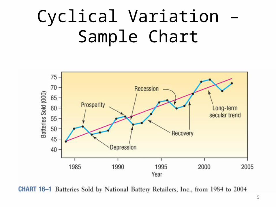
Cyclical Variation – Sample Chart
5
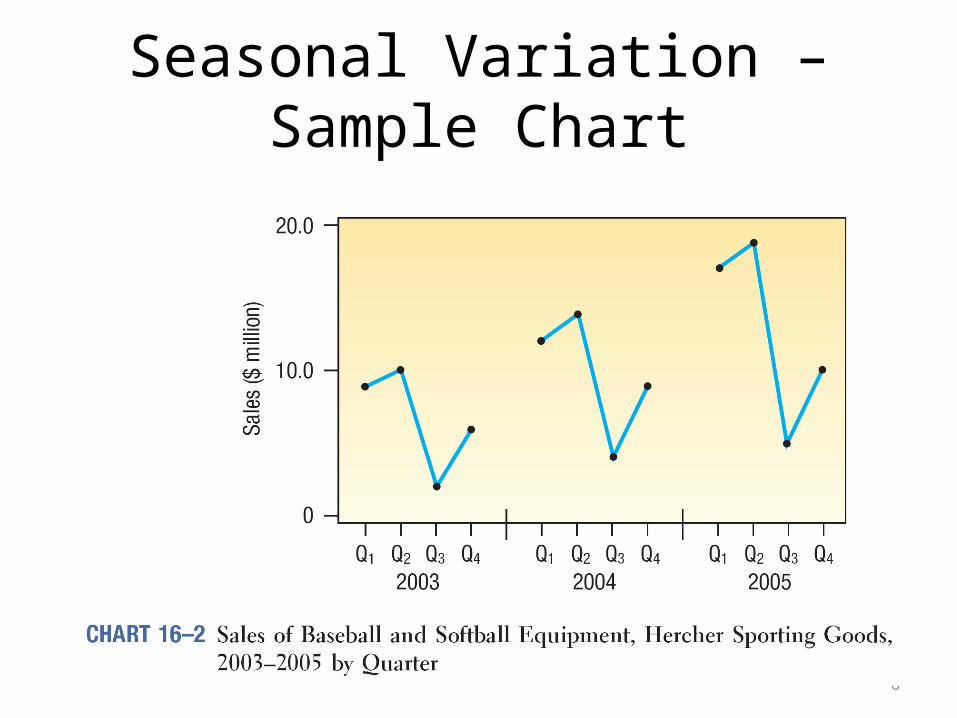
Seasonal Variation – Sample Chart
6

Secular Trend – Home Depot Example
7
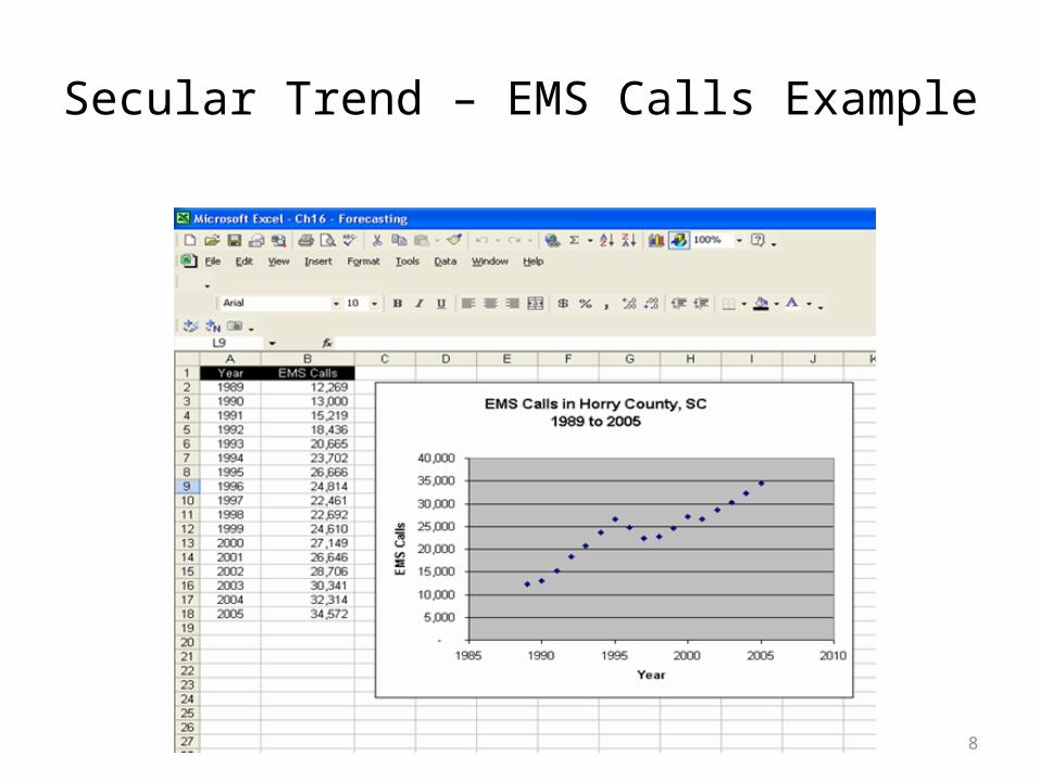
Secular Trend – EMS Calls Example
8
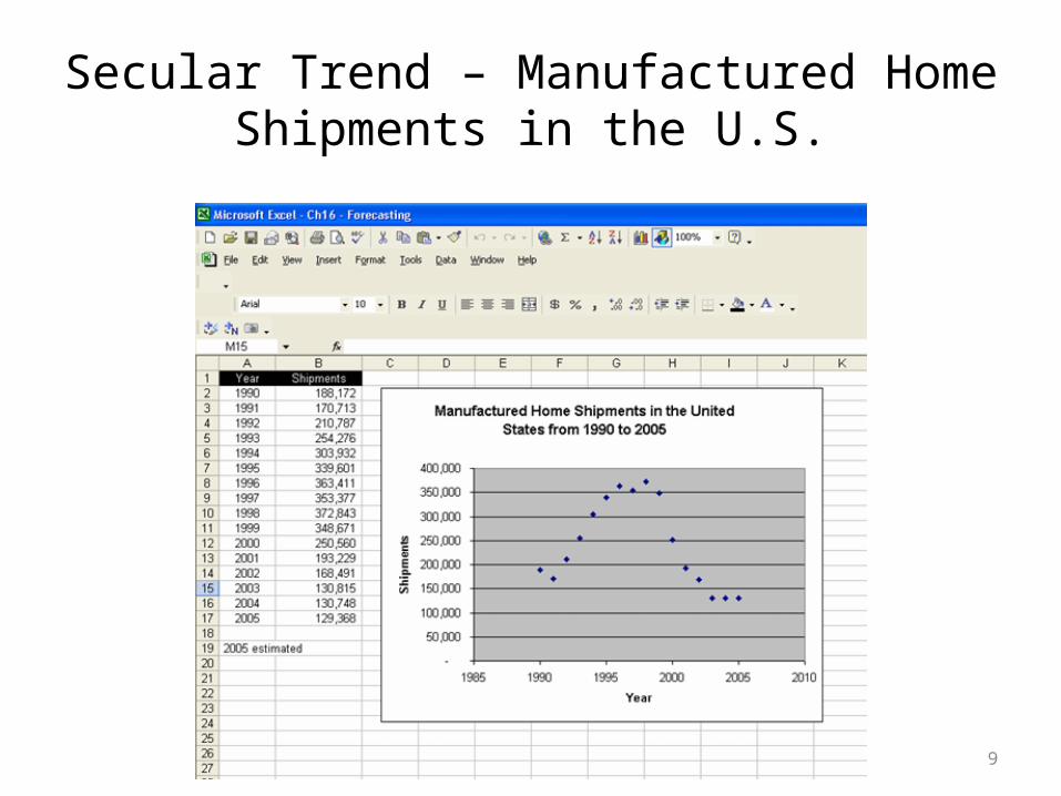
Secular Trend – Manufactured Home Shipments in the U.S.
9
The Moving Average Method
• Useful in smoothing time series to see its trend
• Basic method used in measuring seasonal fluctuation
• Applicable when time series follows fairly linear trend that have definite rhythmic pattern
10
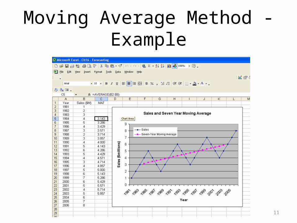
Moving Average Method - Example
11
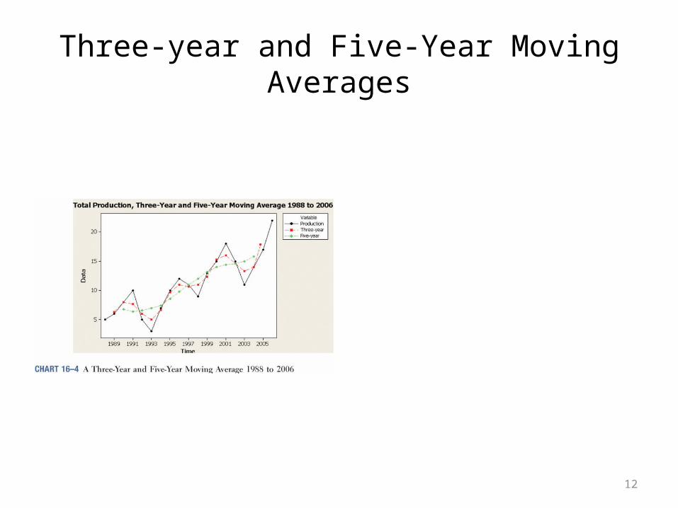
Three-year and Five-Year Moving Averages
12

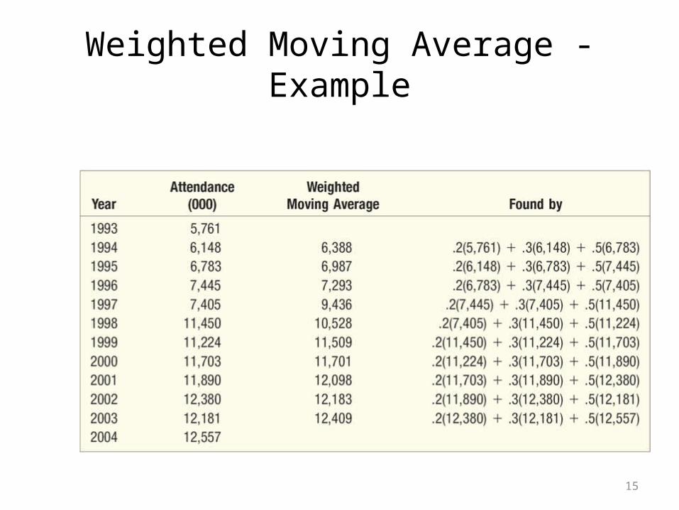
Weighted Moving Average
• A simple moving average assigns the same weight to each observation in averaging
• Weighted moving average assigns different weights to each observation
• Most recent observation receives the most weight, and the weight decreases for older data values
• In either case, the sum of the weights = 1
13
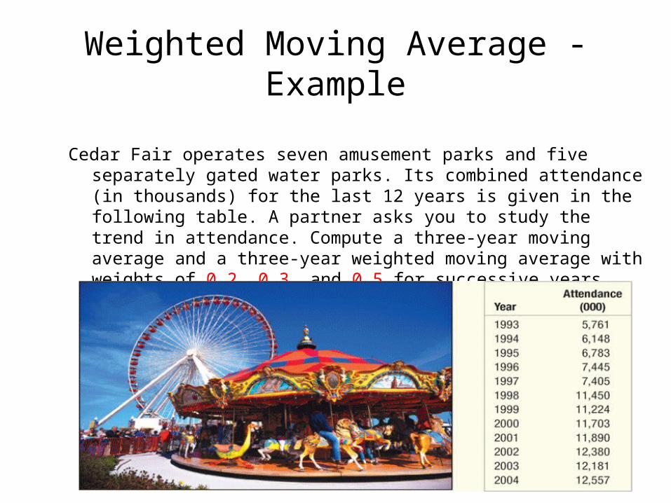
Weighted Moving Average - Example
Cedar Fair operates seven amusement parks and five separately gated water parks. Its combined attendance (in thousands) for the last 12 years is given in the following table. A partner asks you to study the trend in attendance. Compute a three-year moving average and a three-year weighted moving average with weights of 0.2, 0.3, and 0.5 for successive years.
14
Weighted Moving Average - Example
15
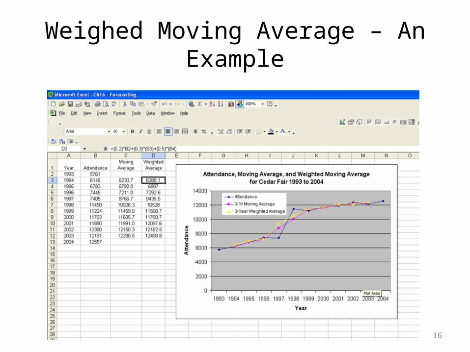
Weighed Moving Average – An Example
16
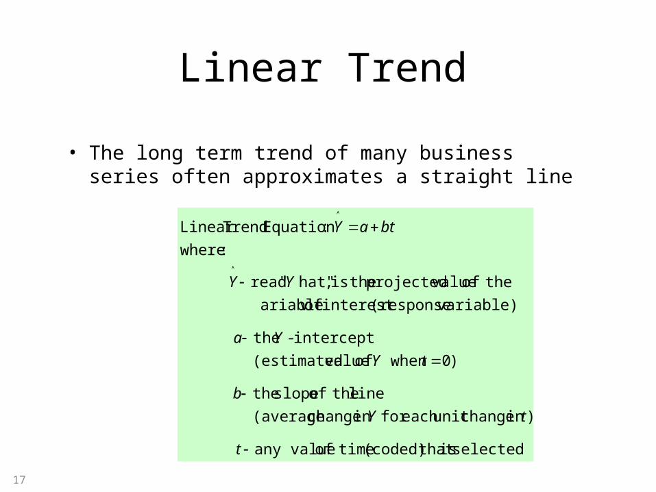
Linear Trend
• The long term trend of many business series often approximates a straight line
selected is that (coded) timeof any value
)in changeunit each for in change (average
line theof slope the
)0 when of value(estimated
intercept - the
variable)(responseinterest of ariable v
theof valueprojected theis ,hat" " read
:where
:Equation TrendLinear
t
tY
b
tY
Ya
YY
btaY
17
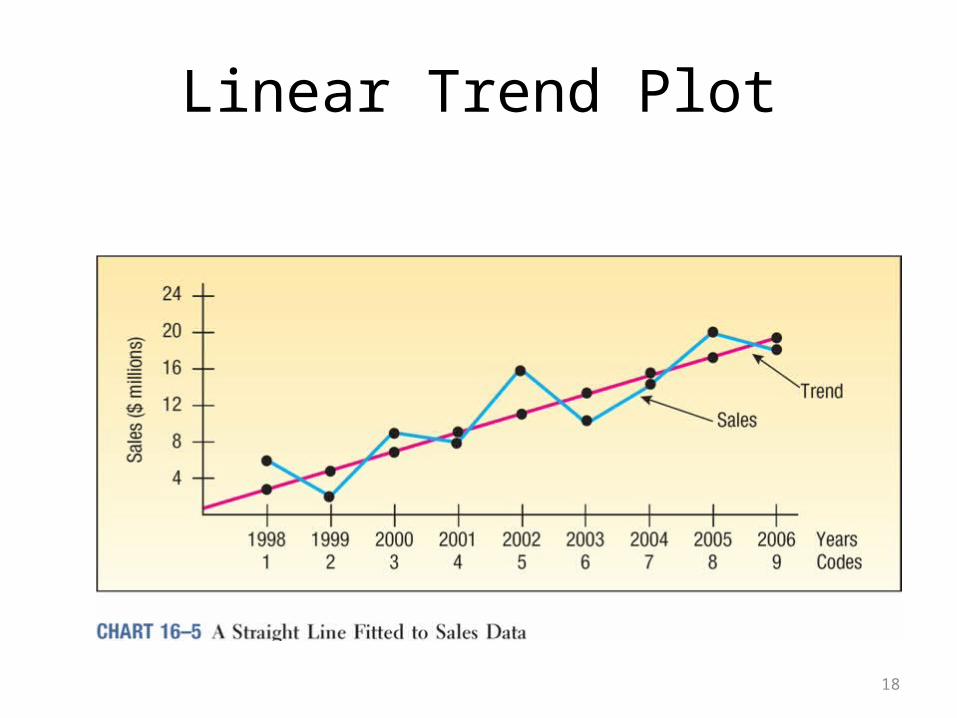
Linear Trend Plot
18

Linear Trend – Using the Least Squares Method
• Use the least squares method in Simple Linear Regression (Chapter 13) to find the best linear relationship between 2 variables
• Code time (t) and use it as the independent variable• E.g. let t be 1 for the first year, 2 for the second, and
so on (if data are annual)
19
Year
Sales
($ mil.)
2002 7
2003 10
2004 9
2005 11
2006 13
Year t
Sales
($ mil.)
2002 1 7
2003 2 10
2004 3 9
2005 4 11
2006 5 1320
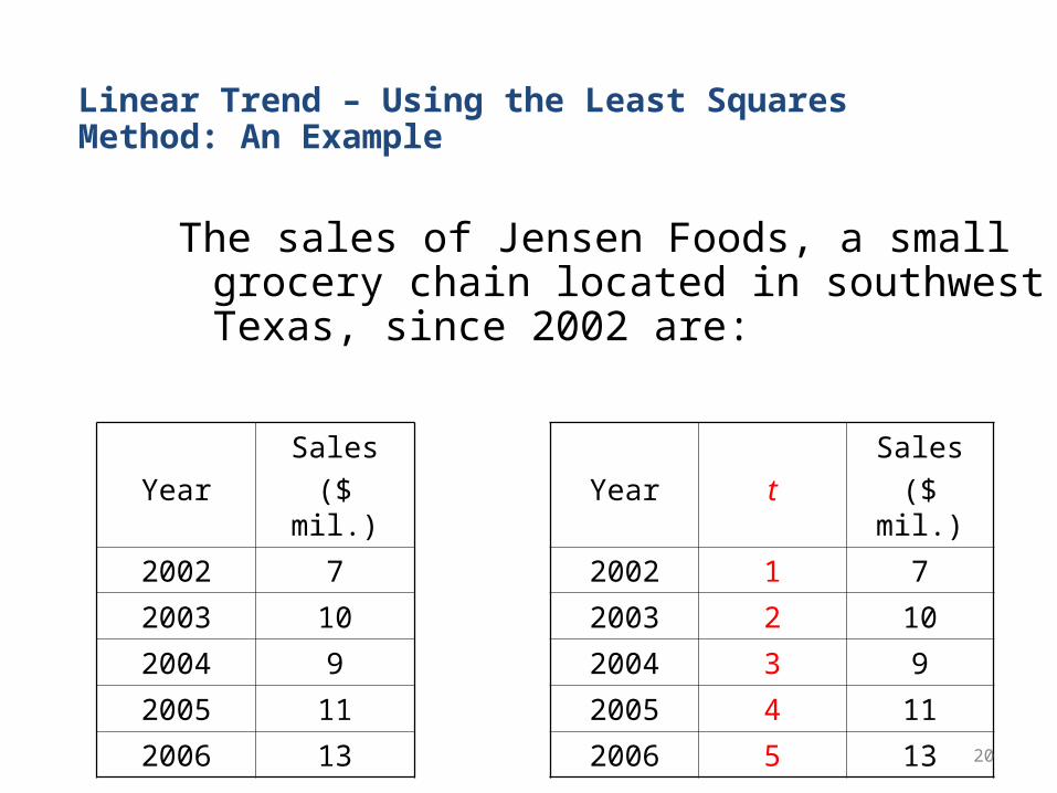
The sales of Jensen Foods, a small grocery chain located in southwest Texas, since 2002 are:
Linear Trend – Using the Least Squares Method: An Example

Linear Trend – Using the Least Squares Method: An Example Using Excel
21
Nonlinear Trends
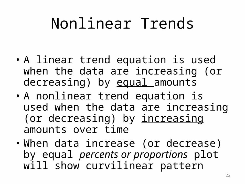
• A linear trend equation is used when the data are increasing (or decreasing) by equal amounts
• A nonlinear trend equation is used when the data are increasing (or decreasing) by increasing amounts over time
• When data increase (or decrease) by equal percents or proportions plot will show curvilinear pattern
22

Log Trend Equation – Gulf Shores Importers Example
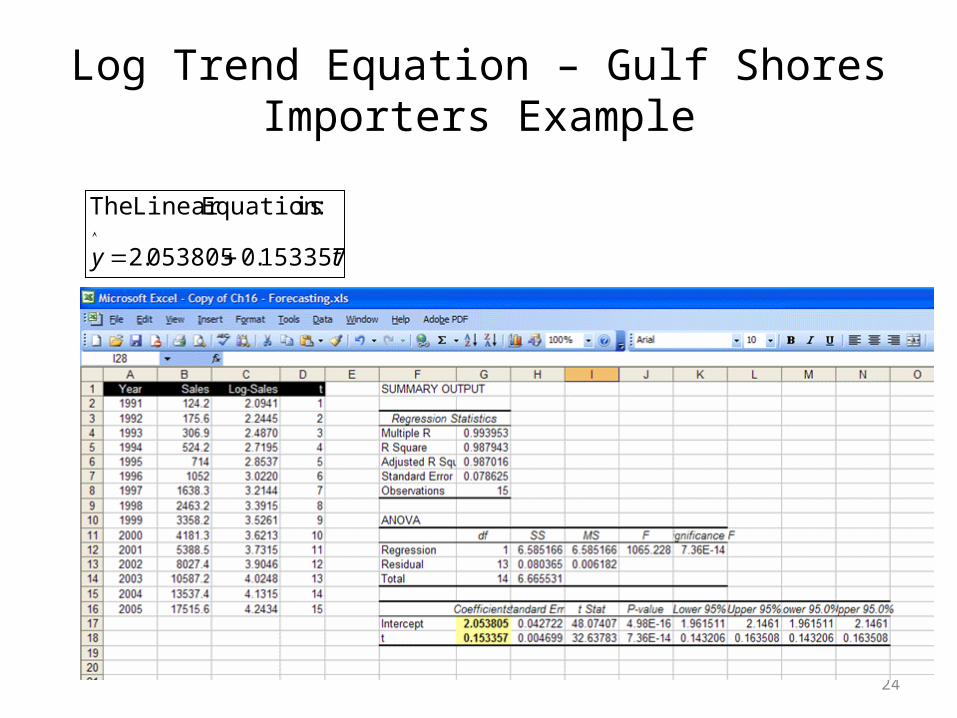
• Top graph is plot of the original data
• Bottom graph is the log base 10 of the original data which now is linear(Excel function:
=log(x) or log(x,10)• Using Data Analysis in
Excel, generate the linear equation
• Regression output shown in next slide
23
Log Trend Equation – Gulf Shores Importers Example
ty 153357.0053805.2
:isEquation Linear The
24
Log Trend Equation – Gulf Shores Importers Example
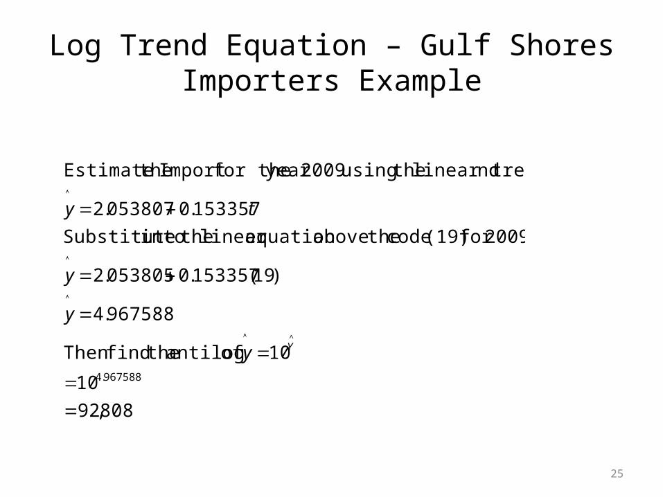
808,92
10
10of antilog thefindThen
967588.4
)19(153357.0053805.2
2009for (19) code theaboveequation linear theinto Substitute
153357.0053807.2
ndlinear tre theusing 2009year for theImport theEstimate
967588.4
^
Yy
y
y
ty
25
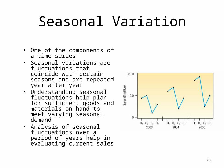
Seasonal Variation
• One of the components of a time series
• Seasonal variations are fluctuations that coincide with certain seasons and are repeated year after year
• Understanding seasonal fluctuations help plan for sufficient goods and materials on hand to meet varying seasonal demand
• Analysis of seasonal fluctuations over a period of years help in evaluating current sales
26
Seasonal Index
• A number, usually expressed in percent, that expresses the relative value of a season with respect to the average for the year (100%)
• Ratio-to-moving-average method – The method most commonly used to compute the
typical seasonal pattern– It eliminates the trend (T), cyclical (C), and
irregular (I) components from the time series
27
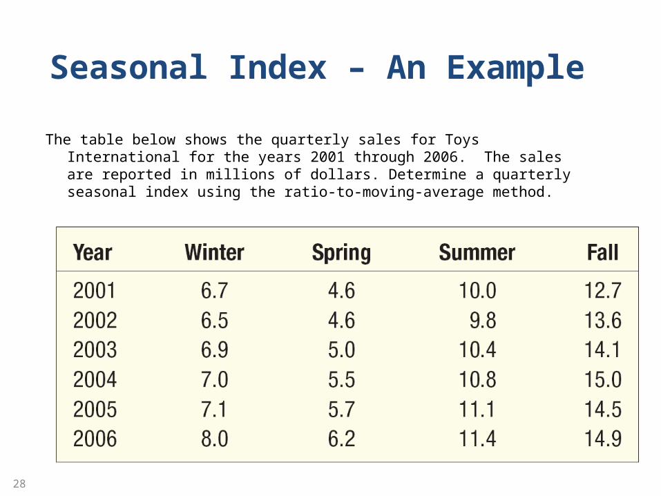
The table below shows the quarterly sales for Toys International for the years 2001 through 2006. The sales are reported in millions of dollars. Determine a quarterly seasonal index using the ratio-to-moving-average method.
28
Seasonal Index – An Example
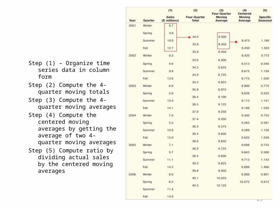
Step (1) – Organize time series data in column form
Step (2) Compute the 4-quarter moving totals
Step (3) Compute the 4-quarter moving averages
Step (4) Compute the centered moving averages by getting the average of two 4-quarter moving averages
Step (5) Compute ratio by dividing actual sales by the centered moving averages
29
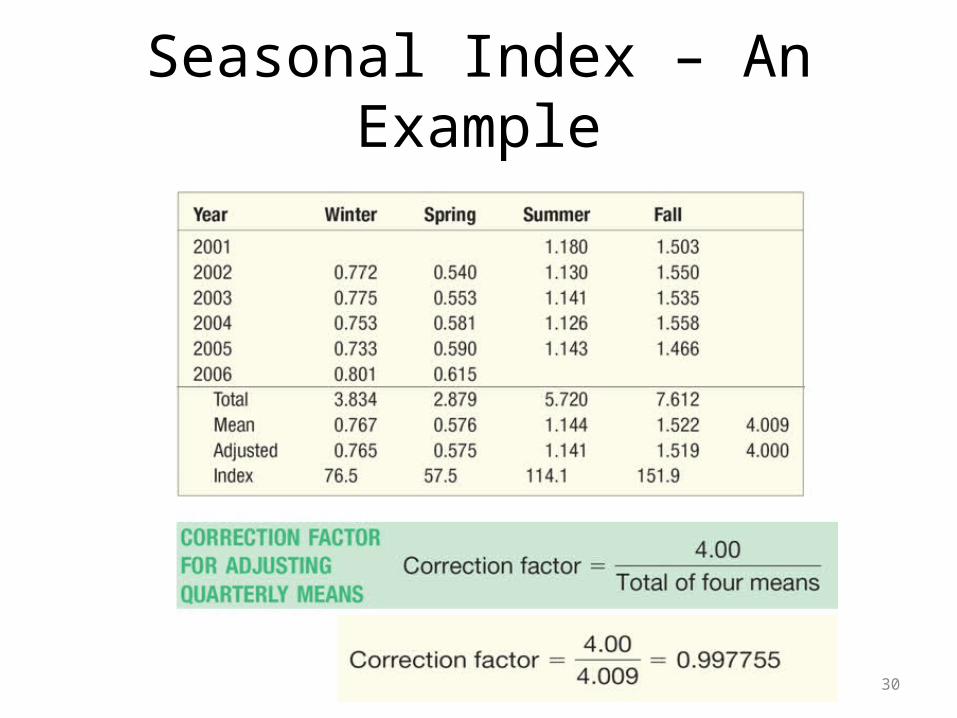
Seasonal Index – An Example
30

Actual versus Deseasonalized Sales for Toys International
Deseasonalized Sales = Sales / Seasonal Index
31

Actual versus Deseasonalized Sales for Toys International – Time Series Plot using Minitab
32
33
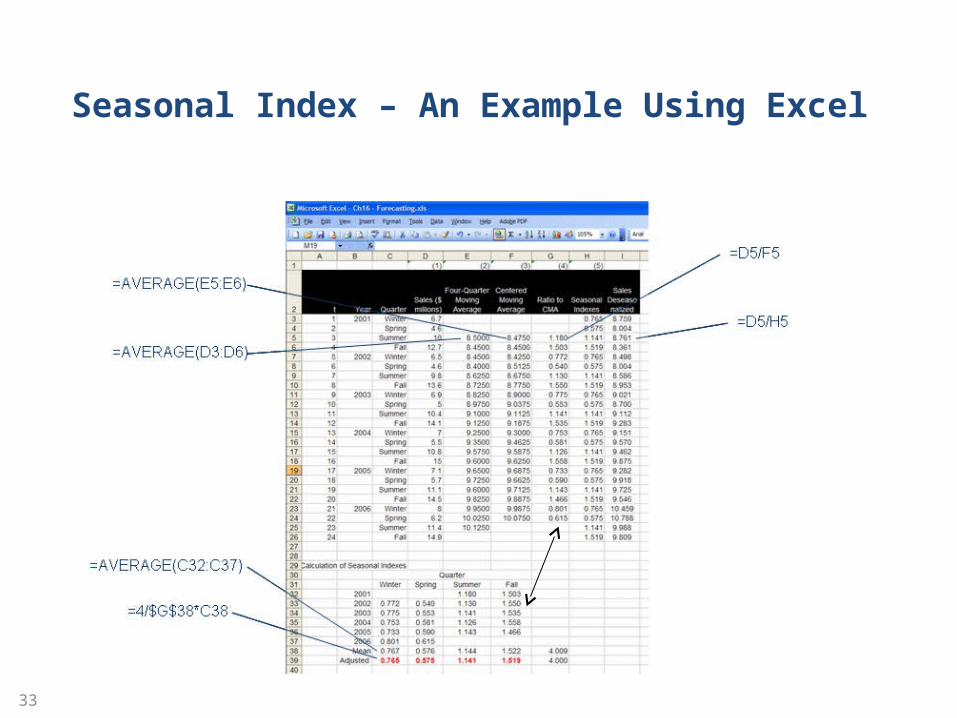
Seasonal Index – An Example Using Excel

34
Seasonal Index – An Example Using Excel
35
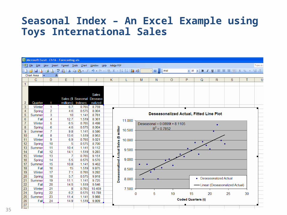
Seasonal Index – An Excel Example using Toys International Sales
Seasonal Index – An Example Using Excel
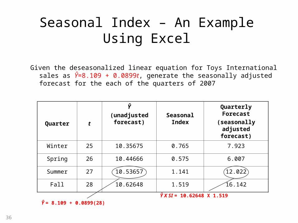
Given the deseasonalized linear equation for Toys International sales as Ŷ=8.109 + 0.0899t, generate the seasonally adjusted forecast for the each of the quarters of 2007
Quarter t
Ŷ
(unadjusted forecast)
Seasonal Index
Quarterly Forecast
(seasonally adjusted forecast)
Winter 25 10.35675 0.765 7.923
Spring 26 10.44666 0.575 6.007
Summer 27 10.53657 1.141 12.022
Fall 28 10.62648 1.519 16.142
36
Ŷ = 8.109 + 0.0899(28)
Ŷ X SI = 10.62648 X 1.519
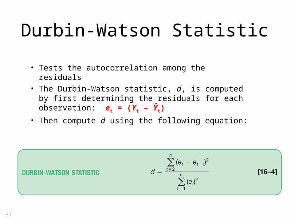
Durbin-Watson Statistic
• Tests the autocorrelation among the residuals• The Durbin-Watson statistic, d, is computed by first
determining the residuals for each observation: et = (Yt – Ŷt)
• Then compute d using the following equation:
37
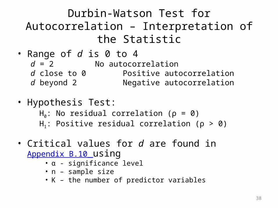
Durbin-Watson Test for Autocorrelation – Interpretation of the Statistic
• Range of d is 0 to 4d = 2 No autocorrelationd close to 0 Positive autocorrelationd beyond 2 Negative autocorrelation
• Hypothesis Test:H0: No residual correlation (ρ = 0)H1: Positive residual correlation (ρ > 0)
• Critical values for d are found in Appendix B.10 using• α - significance level• n – sample size• K – the number of predictor variables
38
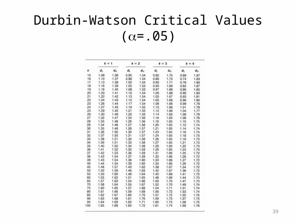
Durbin-Watson Critical Values (=.05)
39
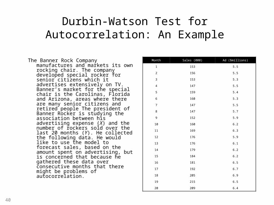
Durbin-Watson Test for Autocorrelation: An Example
The Banner Rock Company manufactures and markets its own rocking chair. The company developed special rocker for senior citizens which it advertises extensively on TV. Banner’s market for the special chair is the Carolinas, Florida and Arizona, areas where there are many senior citizens and retired people The president of Banner Rocker is studying the association between his advertising expense (X) and the number of rockers sold over the last 20 months (Y). He collected the following data. He would like to use the model to forecast sales, based on the amount spent on advertising, but is concerned that because he gathered these data over consecutive months that there might be problems of autocorrelation.
Month Sales (000) Ad ($millions)
1 153 5.5
2 156 5.5
3 153 5.3
4 147 5.5
5 159 5.4
6 160 5.3
7 147 5.5
8 147 5.7
9 152 5.9
10 160 6.2
11 169 6.3
12 176 5.9
13 176 6.1
14 179 6.2
15 184 6.2
16 181 6.5
17 192 6.7
18 205 6.9
19 215 6.5
20 209 6.4
40
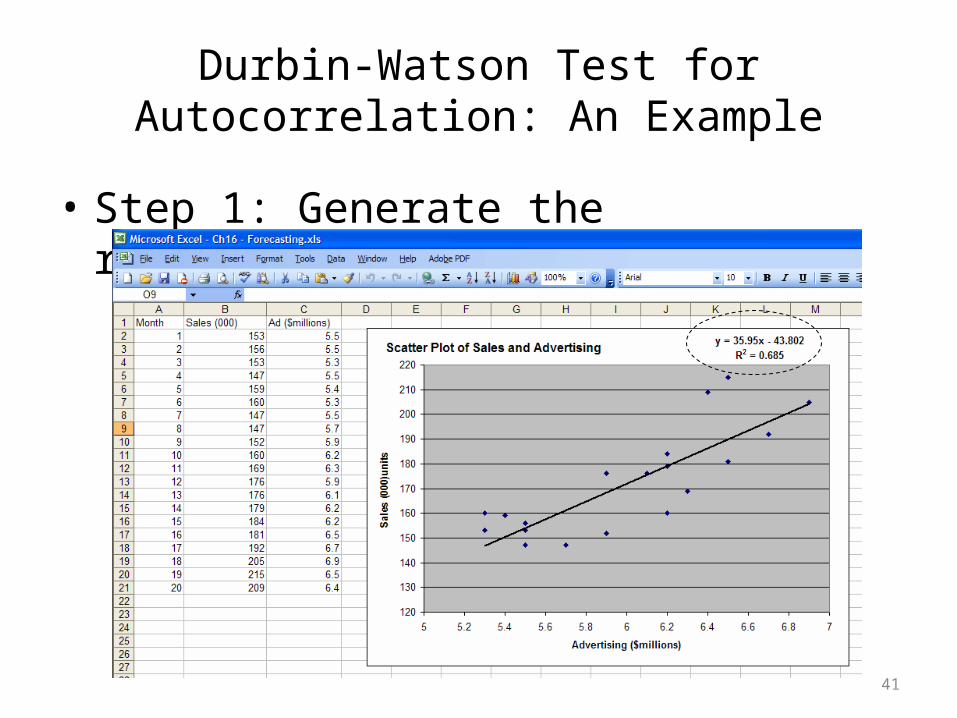
Durbin-Watson Test for Autocorrelation: An Example
• Step 1: Generate the regression equation
41

Durbin-Watson Test for Autocorrelation: An Example
• The resulting equation is: Ŷ = - 43.802 + 35.95X• The coefficient (r) is 0.828• The coefficient of determination (r2) is 68.5%
(note: Excel reports r2 as a ratio. Multiply by 100 to convert into percent)
• There is a strong, positive association between sales and advertising
• Is there potential problem with autocorrelation?
42
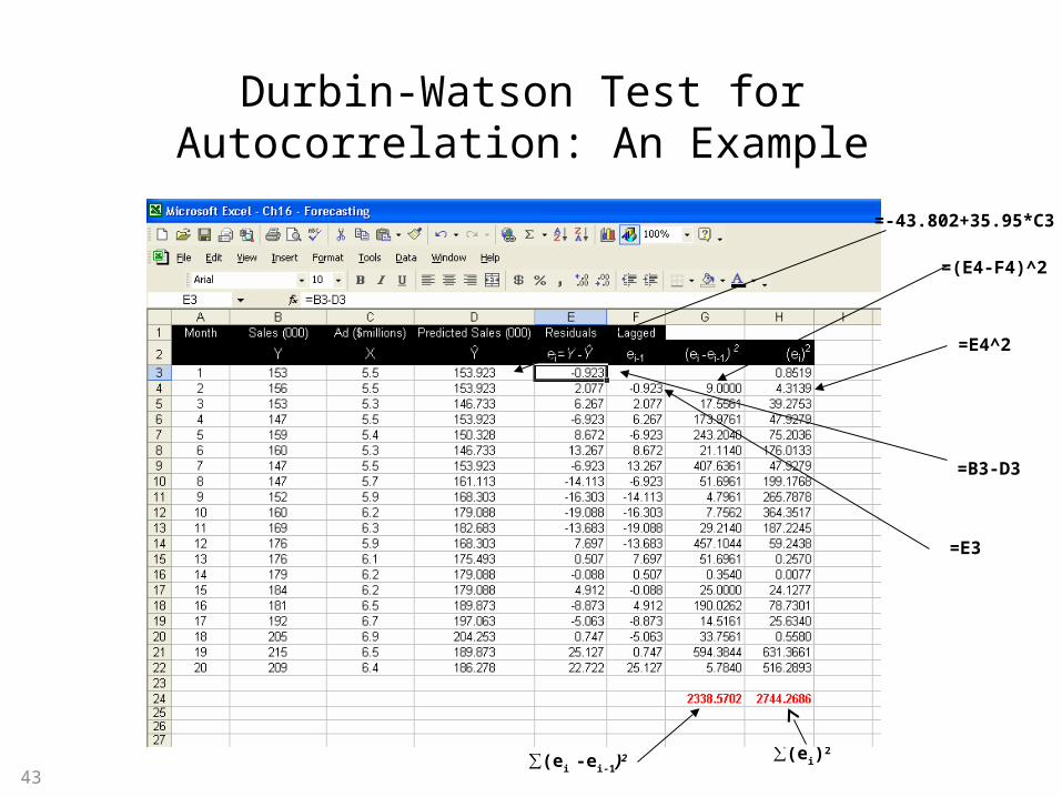
Durbin-Watson Test for Autocorrelation: An Example
∑(ei -ei-1)2 ∑(ei)
2
43
=E4^2
=(E4-F4)^2
=-43.802+35.95*C3
=B3-D3
=E3
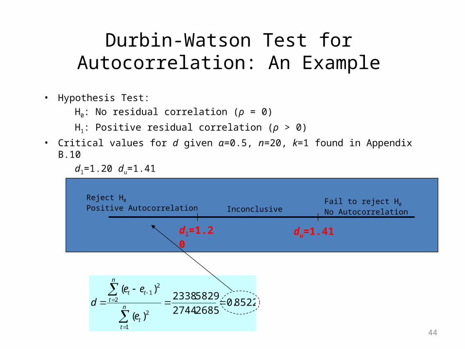
Durbin-Watson Test for Autocorrelation: An Example
• Hypothesis Test:H0: No residual correlation (ρ = 0)
H1: Positive residual correlation (ρ > 0)
• Critical values for d given α=0.5, n=20, k=1 found in Appendix B.10dl=1.20 du=1.41
44
8522.02685.2744
5829.2338
)(
)(
1
2
2
21
n
tt
n
ttt
e
eed
dl=1.20 du=1.41
Reject H0
Positive Autocorrelation InconclusiveFail to reject H0
No Autocorrelation

End of Lesson 12Refer to textbook Chapter 16
45