The maximum entropy approach for aposteriori estimation of model and

data errorsSvetlana Losa

Alfred Wegener Institute for Polar and Marine ResearchBremerhaven, Germany

Thanks to Gennady Kivman, Jens Schröter, Sergey Danilov, Vladimir Ryabchenko, Frank Janssen, Tijana Janjić

))0(()()),0(|)(()),(( 0 xppxtxCptx fft !!!! =

!

Lp (x) = F,

Data assimilation in oceanography (state xi and parameter estimation)

Dynamical model L is model operator

uncertainies in nitial condition x(0), model parameters p, external forcing F

Observational data H is observational operator

We are not confident about the model and data uncertainties.

Do we need the uncertainties quantification?

defined on a Xt×P space, x(t)∈ Xt, p∈P

!

H(x) = d,

!

"(x, p | d) = C"(d | x)"(x, p)

!

"(x, p) = C"(p)"0(x(0)) " f (x(k#t) | x((k $1)#t), p)k=1

M

%

!

He(") = # "(x | d)X$ ln "(x | d)

µ(x)dx%

Principle of Maximum Entropy (general formulation, Kivman et al., 2001)

!

xi = Mmxm + Md xd

!

Mm + Md = I!

Mm = L*L,

!

He(M) = "trace(Md lnMd + Mm lnMm ) = " [#i ln#i + (1" #i)ln(1" #i)]i=1

N

$

!

Md = H*H

!

(xi) = Argmin [L(x, t) " F(t)]2dt0

T# + $ (H(x) " d)2

m=1

M%&

' (

) * +

µ(x) is the lowest information about x.The maximum probable x or mean with respect to ρ(x|d) is

L*, H* reflect our assumptions on the model and data error covariances.Operators Mm and Md are nonnegative, self-adjoint and

M is an operator-valued measure.

We have to find β which would maximize He(M) … or correspondent term in the cost function (Maximum Data Cost, MDC)

Popova’s Ecosystem Model (1995) (generalized inversion)

PhytoplanktonPhytoplankton

ZooplanktonZooplankton

NutrientsNutrients

DetritusDetritus

The flow network between 4 biogeochemical {P, Z, N, D}The flow network between 4 biogeochemical {P, Z, N, D}components, components, xx, possesses , possesses 1919 biological biological parameters,parameters, p p..

66 of them have been of them have been adjustedadjusted for each cell of 5 for each cell of 500x5x500 grid gridcovering the North Atlanticcovering the North Atlantic

Assimilated data:Monthly mean satellite CZCS surface chlorophyll averagedover 1979 – 1985.

Solar irradiation

Method : a weak constraintvariational technique(Losa et al, 2004)

!

(x, p) = Argmin [dxdt

" Lp (x)]2dt

0

T# + $ (H(x) " d)2

m=1

M%

& ' (

) * +

!

r =" H(x) # d 2

m=1

M$dxdt

# Lp (x)%

& ' (

) *

2

dt0

T+

Inference about the model and the data (Which is better: the model or the data)

P

The ratio of the terms in the cost function

Annual model equation residuals normalizedby the total biological source ⇒

P

Z

D

N

!

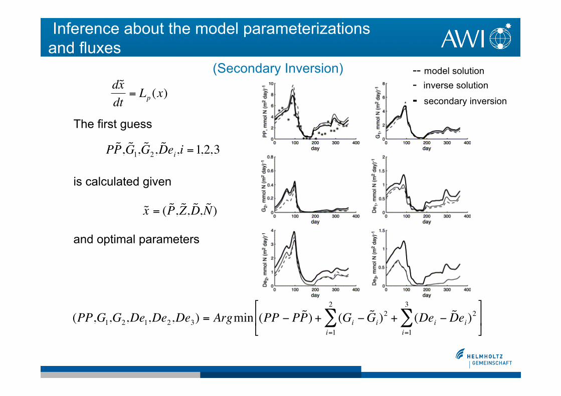
(PP,G1,G2,De1,De2,De3) = Argmin (PP " P ˜ P ) + (Gi " ˜ G i)2 + (Dei " ˜ D ei)

2

i=1

3

#i=1

2

#$

% &

'

( )

Inference about the model parameterizations and fluxes (Secondary Inversion)

!

˜ x = ( ˜ P , ˜ Z , ˜ D , ˜ N )

The first guess

is calculated given

and optimal parameters

!

P ˜ P , ˜ G 1, ˜ G 2, ˜ D ei,i =1,2,3!

d˜ x dt

= Lp (x)

-- model solution- inverse solution

- secondary inversion

August horizontal distribution of the surfacechlorophyll “a” in the North Atlantic

(Popova’s NPZD coupled to 3D POP gcm)

Losa et al., 2006

Model with const param SeaWiFs dataModel with variable param

Annual composite of classified coccolithophorid blooms in SeaWiFS imagery dating from October 1997 to September 1999 ( (Iglesias-Rodríguez et al., 2002)

The bloom class is white, the non-coccolithophorid bloom class is blue, the land is black, and ice is gray.

Strong thermal stratification

Water temperature between 50C and 150C

High solar radiation (low values of α parameter)

Declining nutrients

Decreasing zooplankton grazing pressure (escaping grazing control)

Assimilating NOAA’s SST data into an operationalcirculation model of the North and Baltic Seas

BSHcmodNOAA SST

Extraction and combination of the information from two different sources - themodel and the data - in order to improve our understanding of both sources

and, therefore, of reality itself

12 hourly-around 00:00 and 12:00,- composites of SST measured by the Advanced Very High Resolution Radiometer (AVHRR)aboard polar orbiting satellites

ρta(x(t1|d1)=Cρd(d1|x(t1)ρt

f(x(t1))ρt

f(x(t1)=Cρf(x(t)|x(0))ρ0(x(0))

BSHcmod run at the NOAA SSTGerman Maritime and Hydrographic Agency (BSH)

!

x(tn )a = x(tn )

f ,m +Kn (dn "Hx(tn )f ,m )

Sequantial statistical approach (Kalman type filtering)

!

Kn = Pnf H(HPn

f HT + R)"1

xf, xa denote forecast and analysis of state vector (at time tn at all grid points) dn - observations available (at tn) Pn

f - forecast error covariance matrix R - observational error covariance matrix

SEIK Filter is implemented locally (PDAF, Nerger et al., 2006) but with differentformulations of data error correlation.

When calculating He(M), the Kalman gain K could be considered

globally over a certain period of time locally (for validation of localization conditions)Use SVD decomposition

Ensemble based Singular Evolutive Interpolated Kalman filter (SEIK, Pham, 2001)

Improvement of SST analysis and forecast

Improvement of SST forecast

Experiment He(M)

σsst=0.6 oC 3.99

σsst=0.8 oC 4.33

σsst=1.2 oC 3.90

Comparison with independent information

Experiment He(M)

σsst=0.6 oC 3.99

σsst=0.8 oC 4.33

σsst=1.2 oC 3.90

Sensitivity of the forecast quality

Experiment He(M)

σsst=0.6oC, Pfs 3.57

σsst=0.8oC, Pfs 4.17

σsst=0.8oC 4.33

Comparison with independent information

Experiment He(M)

σsst=0.6oC, Pfs 3.57

σsst=0.8oC, Pfs 4.17

σsst=0.8oC 4.33

Comparison with independent information

Deviation from MARNET SST Daten

Station RMS (oC) Bias (oC) Model LSEIK NOAA Model LSEIK NOAA Arkona 0.88 0.58 0.61 -0.29 0. 0.04 Darβ 1.27 0.81 0.69 -0.55 -0.17 0.01 Kiel 0.79 0.49 0.61 -0.13 0.07 0.08 Fehm 0.63 0.43 0.56 -0.16 0.03 0.16 Ems 0.67 0.45 0.49 0.33 0.2 0.17 Dbucht 0.97 0.53 0.57 -0.34 -0.03 0.27 nsb 0.73

Normaler Text

Increment Analysis

Improvement of SST forecast in the North and the BalticSeas when sequentially assimilating satellite data

Bias reduction

Bias without DA with LSEIK filter

ConclusionsWe have demonstrated two examples of the PME implementation for a posteriori estimating the modeland data errors in data assimilation problem.

The chlorophyll satellite data assimilation based on a posteriori choosing of the data weight allowed usto compare the quality of the data and ecosystem model prediction and discern the low quality of thesatellite data for high latitudes and for the coastal region of the North Atlantic.

The procedure of the secondary inversion of biogeochemical fluxes makes it possible to restore themass balance broken while performing the weak constraint parameter estimation and to refine theestimates of the biogeochemical fluxes.

The spatial distribution of the biogeochemical parameters is in a good agreement with independentinformation about spices composition/distribution and their physiology.

Implementation of the PME for assessing prior model and data error statistics in SST data ensemblebased assimilation for an operational forecasting model of the North and Baltic Seas revealed the bestagreement of the forecast with independent data under the assumptions on initial model and data errorstatistics, which produced the ME of the posterior distribution.

Investigation of the PME implementation in a local analysis content is of our further interest.

ReferencesBoltzmann, L., 1964: Lectures on Gas Theory. Cambridge University Press, 490 pp. [First published asVorlesungen über Gastheorie, Barth, 1896.].

Gibbs, J. W., 1902: Elementary Principles in Statistical Mechanics. Yale University Press, 207 pp.

Kivman, G. A., Kurapov, A. L., Guessen, A. V., 2001: An Entropy Approach to Tuning Weights andSmoothing in the Generalized Inversion. J. Atmos. Oceanic Technol., 18, 266–276.

Losa, S. N, Kivman, G. A., Ryabchenko, V. A., 2004: Weak constraint parameter estimation for a simpleocean ecosystem model: what can we learn about the model and data?, Journal of Marine Systems, Volume45, Issues 1-2, Pages 1-20, ISSN 0924-7963, 10.1016/j.jmarsys.2003.08.005.

Losa, S. N., Vézina, A., Wright, D., Lu, Y., Thompson, K., Dowd, M., 2006: 3D ecosystem modelling in theNorth Atlantic: Relative impacts of physical and biological parameterizations. Journal of Marine Systems,Volume 61, Issues 3-4, Pages 230-245, ISSN 0924-7963, 10.1016/j.jmarsys.2005.09.011.

Nerger, L., S. Danilov, W. Hiller, and J. Schröter. Using sea level data to constrain a finite-element primitive-equation model with a local SEIK filter. Ocean Dynamics 56 (2006) 634

Shannon, C. E., 1948: A mathematical theory of communication. Bell Syst. Tech. J.,27, 379–423, 623–655.

Tarantola, A., 1987: Inverse Problem Theory: Methods for Data Fitting and Model Parameter Estimation.Elsevier, 613 pp.

van Leeuwen, P. J., and G. Evensen, 1996: Data assimilation and inverse methods in terms of aprobabilistic formulation. Mon. Wea. Rev.,124, 2898–2913.