The Matplotlib User’s Guide

John Hunterand

Darren Dale

March 3, 2007

2

Contents

1 Introduction 51.1 Migrating from MATLABTM . . . . . . . . . . . . . . . . . . . . . . . . . . . . . . . . . . . . . . . 6

2 Installation and Setup 92.1 Installing . . . . . . . . . . . . . . . . . . . . . . . . . . . . . . . . . . . . . . . . . . . . . . . . . 9

2.1.1 Quickstart on windows . . . . . . . . . . . . . . . . . . . . . . . . . . . . . . . . . . . . . . 92.1.2 Package managers: (rpms, apt, fink) . . . . . . . . . . . . . . . . . . . . . . . . . . . . . . . 92.1.3 Compiling matplotlib . . . . . . . . . . . . . . . . . . . . . . . . . . . . . . . . . . . . . . . 102.1.4 Trial Run . . . . . . . . . . . . . . . . . . . . . . . . . . . . . . . . . . . . . . . . . . . . . 11

2.2 Backends . . . . . . . . . . . . . . . . . . . . . . . . . . . . . . . . . . . . . . . . . . . . . . . . . 112.3 Integrated development environments . . . . . . . . . . . . . . . . . . . . . . . . . . . . . . . . . . 122.4 Interactive . . . . . . . . . . . . . . . . . . . . . . . . . . . . . . . . . . . . . . . . . . . . . . . . . 132.5 Numerix . . . . . . . . . . . . . . . . . . . . . . . . . . . . . . . . . . . . . . . . . . . . . . . . . . 14

2.5.1 Choosing Numeric, numarray, or NumPy . . . . . . . . . . . . . . . . . . . . . . . . . . . . 142.6 Customization using matplotlibrc . . . . . . . . . . . . . . . . . . . . . . . . . . . . . . . . . . . 15

2.6.1 RC file format . . . . . . . . . . . . . . . . . . . . . . . . . . . . . . . . . . . . . . . . . . 152.6.2 Which rc file is used? . . . . . . . . . . . . . . . . . . . . . . . . . . . . . . . . . . . . . . . 152.6.3 In the event of a problem . . . . . . . . . . . . . . . . . . . . . . . . . . . . . . . . . . . . . 16

3 The pylab interface 173.1 Simple plots . . . . . . . . . . . . . . . . . . . . . . . . . . . . . . . . . . . . . . . . . . . . . . . . 173.2 More on plot . . . . . . . . . . . . . . . . . . . . . . . . . . . . . . . . . . . . . . . . . . . . . . . 19

3.2.1 Multiple lines . . . . . . . . . . . . . . . . . . . . . . . . . . . . . . . . . . . . . . . . . . . 193.2.2 Controlling line properties . . . . . . . . . . . . . . . . . . . . . . . . . . . . . . . . . . . . 20

3.3 Color arguments . . . . . . . . . . . . . . . . . . . . . . . . . . . . . . . . . . . . . . . . . . . . . . 223.4 Loading and saving data . . . . . . . . . . . . . . . . . . . . . . . . . . . . . . . . . . . . . . . . . 22

3.4.1 Loading and saving ASCII data . . . . . . . . . . . . . . . . . . . . . . . . . . . . . . . . . 223.4.2 Loading and saving binary data . . . . . . . . . . . . . . . . . . . . . . . . . . . . . . . . . 233.4.3 Processing several data files . . . . . . . . . . . . . . . . . . . . . . . . . . . . . . . . . . . 24

3.5 axes and figures . . . . . . . . . . . . . . . . . . . . . . . . . . . . . . . . . . . . . . . . . . . . . . 243.5.1 figure . . . . . . . . . . . . . . . . . . . . . . . . . . . . . . . . . . . . . . . . . . . . . . 243.5.2 subplot . . . . . . . . . . . . . . . . . . . . . . . . . . . . . . . . . . . . . . . . . . . . . 253.5.3 axes . . . . . . . . . . . . . . . . . . . . . . . . . . . . . . . . . . . . . . . . . . . . . . . 27

3.6 Text . . . . . . . . . . . . . . . . . . . . . . . . . . . . . . . . . . . . . . . . . . . . . . . . . . . . 293.6.1 Basic text commands . . . . . . . . . . . . . . . . . . . . . . . . . . . . . . . . . . . . . . . 293.6.2 Text properties . . . . . . . . . . . . . . . . . . . . . . . . . . . . . . . . . . . . . . . . . . 293.6.3 Text layout . . . . . . . . . . . . . . . . . . . . . . . . . . . . . . . . . . . . . . . . . . . . 303.6.4 mathtext . . . . . . . . . . . . . . . . . . . . . . . . . . . . . . . . . . . . . . . . . . . . . . 32

3.7 Images . . . . . . . . . . . . . . . . . . . . . . . . . . . . . . . . . . . . . . . . . . . . . . . . . . . 343.7.1 Axes images . . . . . . . . . . . . . . . . . . . . . . . . . . . . . . . . . . . . . . . . . . . 34

3

3.7.2 Figure images . . . . . . . . . . . . . . . . . . . . . . . . . . . . . . . . . . . . . . . . . . . 363.7.3 Scaling and color mapping . . . . . . . . . . . . . . . . . . . . . . . . . . . . . . . . . . . . 363.7.4 Image origin . . . . . . . . . . . . . . . . . . . . . . . . . . . . . . . . . . . . . . . . . . . 37

3.8 Bar charts, histograms and errorbar plots . . . . . . . . . . . . . . . . . . . . . . . . . . . . . . . . . 383.9 Pseudocolor and scatter plots . . . . . . . . . . . . . . . . . . . . . . . . . . . . . . . . . . . . . . . 383.10 Spectral analysis . . . . . . . . . . . . . . . . . . . . . . . . . . . . . . . . . . . . . . . . . . . . . 383.11 Axes properties . . . . . . . . . . . . . . . . . . . . . . . . . . . . . . . . . . . . . . . . . . . . . . 403.12 Legends and tables . . . . . . . . . . . . . . . . . . . . . . . . . . . . . . . . . . . . . . . . . . . . 403.13 Navigation . . . . . . . . . . . . . . . . . . . . . . . . . . . . . . . . . . . . . . . . . . . . . . . . . 40

3.13.1 Classic toolbar . . . . . . . . . . . . . . . . . . . . . . . . . . . . . . . . . . . . . . . . . . 403.13.2 toolbar2 . . . . . . . . . . . . . . . . . . . . . . . . . . . . . . . . . . . . . . . . . . . . . . 40

3.14 Event handling . . . . . . . . . . . . . . . . . . . . . . . . . . . . . . . . . . . . . . . . . . . . . . 423.15 Customizing plot defaults . . . . . . . . . . . . . . . . . . . . . . . . . . . . . . . . . . . . . . . . . 43

4 Font finding and properties 45

5 Collections 49

6 Tick locators and formatters 516.1 Tick locating . . . . . . . . . . . . . . . . . . . . . . . . . . . . . . . . . . . . . . . . . . . . . . . 516.2 Tick formatting . . . . . . . . . . . . . . . . . . . . . . . . . . . . . . . . . . . . . . . . . . . . . . 526.3 Example 1: major and minor ticks . . . . . . . . . . . . . . . . . . . . . . . . . . . . . . . . . . . . 526.4 Example 2: date ticking . . . . . . . . . . . . . . . . . . . . . . . . . . . . . . . . . . . . . . . . . . 54

7 Cookbook 577.1 Plot elements . . . . . . . . . . . . . . . . . . . . . . . . . . . . . . . . . . . . . . . . . . . . . . . 57

7.1.1 Horizontal or vertical lines/spans . . . . . . . . . . . . . . . . . . . . . . . . . . . . . . . . . 577.1.2 Fill the area between two curves . . . . . . . . . . . . . . . . . . . . . . . . . . . . . . . . . 57

7.2 Text . . . . . . . . . . . . . . . . . . . . . . . . . . . . . . . . . . . . . . . . . . . . . . . . . . . . 577.2.1 Adding a ylabel on the right of the axes . . . . . . . . . . . . . . . . . . . . . . . . . . . . . 57

7.3 Data analysis . . . . . . . . . . . . . . . . . . . . . . . . . . . . . . . . . . . . . . . . . . . . . . . 587.3.1 Linear regression . . . . . . . . . . . . . . . . . . . . . . . . . . . . . . . . . . . . . . . . . 587.3.2 Polynomial regression . . . . . . . . . . . . . . . . . . . . . . . . . . . . . . . . . . . . . . 59

7.4 Working with images . . . . . . . . . . . . . . . . . . . . . . . . . . . . . . . . . . . . . . . . . . . 607.4.1 Loading existing images into matplotlib . . . . . . . . . . . . . . . . . . . . . . . . . . . . . 607.4.2 Blending several axes images using alpha . . . . . . . . . . . . . . . . . . . . . . . . . . . . 617.4.3 Creating a mosaic of images . . . . . . . . . . . . . . . . . . . . . . . . . . . . . . . . . . . 627.4.4 Defining your own colormap . . . . . . . . . . . . . . . . . . . . . . . . . . . . . . . . . . . 63

7.5 Output . . . . . . . . . . . . . . . . . . . . . . . . . . . . . . . . . . . . . . . . . . . . . . . . . . . 637.5.1 Printing to standard output . . . . . . . . . . . . . . . . . . . . . . . . . . . . . . . . . . . . 63

8 Matplotlib API 658.1 The matplotlib backends . . . . . . . . . . . . . . . . . . . . . . . . . . . . . . . . . . . . . . . . . 65

8.1.1 The renderer and graphics context . . . . . . . . . . . . . . . . . . . . . . . . . . . . . . . . 668.1.2 The figure canvases . . . . . . . . . . . . . . . . . . . . . . . . . . . . . . . . . . . . . . . . 67

8.2 The matplotlib Artists . . . . . . . . . . . . . . . . . . . . . . . . . . . . . . . . . . . . . . . . . . . 678.3 pylab interface internals . . . . . . . . . . . . . . . . . . . . . . . . . . . . . . . . . . . . . . . . . . 67

A A sample matplotlibrc 73

B mathtext symbols 79

C matplotlib source code license 81

4

Chapter 1

Introduction

matplotlib is a library for making 2D plots of arrays in python. Although it has its origins in emulating the MATLABTM

graphics commands, it does not require MATLABTM, and can be used in a pythonic, object oriented way. Althoughmatplotlib is written primarily in pure python, it makes heavy use of NumPy and other extension code to provide goodperformance even for large arrays.

matplotlib is designed with the philosophy that you should be able to create simple plots with just a few commands,or just one! If you want to see a histogram of your data, you shouldn’t need to instantiate objects, call methods, setproperties, and so forth; it should just work.

For years, I used to use MATLABTM exclusively for data analysis and visualization. MATLABTM excels at makingit easy to create nice looking plots. When I began working with EEG data, I found that I needed to write applicationsto interact with my data, and developed an EEG analysis application in MATLABTM. As the application grew incomplexity, interacting with databases, http servers, manipulating complex data structures, I began to strain againstthe limitations of MATLABTM as a programming language, and decided to start over in python. python more thanmakes up for all of matlab’s deficiencies as a programming language, but I was having difficulty finding a 2D plottingpackage (for 3D VTK more than exceeds all of my needs).

When I went searching for a python plotting package, I had several requirements:

• Plots should look great - publication quality. One important requirement for me is that the text looks good(antialiased, etc)

• Postscript output for inclusion with TEX documents

• Embeddable in a graphical user interface for application development

• Code should be easy enough that I can understand it and extend it.

• Making plots should be easy.

Finding no package that suited me just right, I did what any self-respecting python programmer would do: rolled upmy sleeves and dived in. Not having any real experience with computer graphics, I decided to emulate MATLABTM’splotting capabilities because that is something MATLABTM does very well. This had an added advantage: manypeople have a lot of MATLABTM experience, and thus they can quickly get up to steam plotting in python. From adeveloper’s perspective, having a fixed, MATLABTM-inspired user interface (the pylab interface) has been very useful,because the guts of the code base can be redesigned without affecting user code.

The matplotlib code is conceptually divided into three parts: the pylab interface is the set of functions providedby matplotlib.pylab which allow the user to create plots with code quite similar to MATLABTM figure generatingcode. The matplotlib frontend or matplotlib API is the set of classes that do the heavy lifting, creating and managingfigures, text, lines, plots and so on. This is an abstract interface that knows nothing about output. The backendsare device dependent drawing devices, aka renderers, that transform the frontend representation to hardcopy or adisplay device. Example backends: PS creates postscript hardcopy, SVG creates scalar vector graphics hardcopy, Agg

5

creates PNG output using the high quality antigrain library that ships with matplotlib - http://antigrain.com, GTKembeds matplotlib in a GTK application, GTKAgg uses the antigrain renderer to create a figure and embed it a GTKapplication, and so on for WX, Tkinter, Qt, FLTK. . . .

matplotlib is used by many people in many different contexts. Some people want to automatically generatepostscript files to send to a printer or publishers. Others deploy matplotlib on a web application server to generatePNG output for inclusion in dynamically generated web pages. Some use matplotlib interactively from the pythonshell in Tkinter on windows. My primary use is to embed matplotlib in a GTK EEG application that runs on windows,linux and OS X.

Because there are so many ways people want to use a plotting library, there is a certain amount of complexityinherent in configuring the library so that it will work naturally the way you want it to. Before diving into these details,let’s first explore matplotlib’s simplicity by comparing a typical matplotlib script with its analog in MATLABTM.

— JDH

1.1 Migrating from MATLABTM

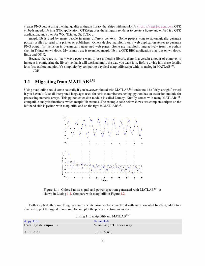
Using matplotlib should come naturally if you have ever plotted with MATLABTM and should be fairly straightforwardif you haven’t. Like all interpreted languages used for serious number crunching, python has an extension module forprocessing numeric arrays. This python extension module is called Numpy. NumPy comes with many MATLABTM-compatible analysis functions, which matplotlib extends. The example code below shows two complete scripts: on theleft hand side is python with matplotlib, and on the right is MATLABTM.

Figure 1.1: Colored noise signal and power spectrum generated with MATLABTM asshown in Listing 1.1. Compare with matplotlib in Figure 1.2.

Both scripts do the same thing: generate a white noise vector, convolve it with an exponential function, add it to asine wave, plot the signal in one subplot and plot the power spectrum in another.

Listing 1.1: matplotlib and MATLABTM

# py thon % ma t l abfrom p y l a b import ∗ % no import n e c e s s a r y

d t = 0 . 0 1 d t = 0 . 0 1 ;

6

t = a r a n g e ( 0 , 1 0 , d t ) t = [ 0 : d t : 1 0 ] ;nse = randn ( l e n ( t ) ) nse = randn ( s i z e ( t ) ) ;r = exp(− t / 0 . 0 5 ) r = exp(− t / 0 . 0 5 ) ;

cnse = conv ( nse , r ) ∗ d t cnse = conv ( nse , r ) ∗ d t ;cnse = cnse [ : l e n ( t ) ] cnse = cnse ( 1 : l e n g t h ( t ) ) ;s = 0 . 1∗ s i n (2∗ p i ∗ t ) + cnse s = 0 . 1∗ s i n (2∗ p i ∗ t ) + cnse ;

s u b p l o t ( 2 1 1 ) s u b p l o t ( 2 1 1 )p l o t ( t , s ) p l o t ( t , s )s u b p l o t ( 2 1 2 ) s u b p l o t ( 2 1 2 )psd ( s , 512 , 1 / d t ) psd ( s , 512 , 1 / d t )

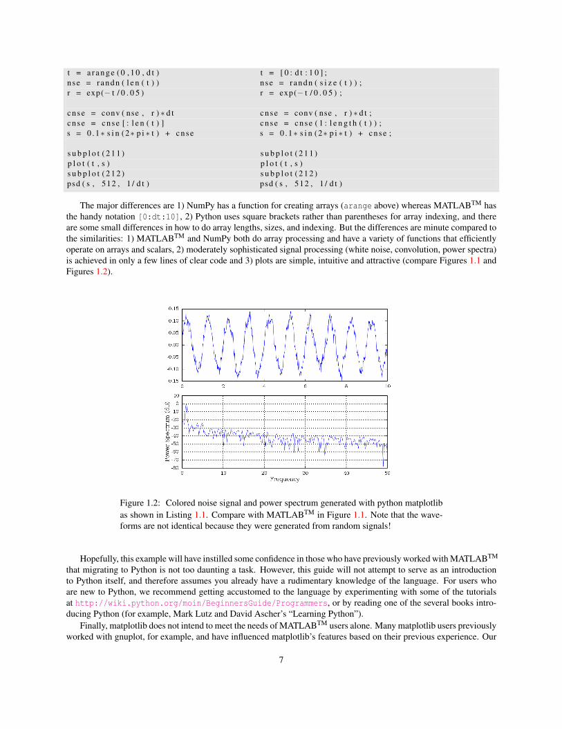
The major differences are 1) NumPy has a function for creating arrays (arange above) whereas MATLABTM hasthe handy notation [0:dt:10], 2) Python uses square brackets rather than parentheses for array indexing, and thereare some small differences in how to do array lengths, sizes, and indexing. But the differences are minute compared tothe similarities: 1) MATLABTM and NumPy both do array processing and have a variety of functions that efficientlyoperate on arrays and scalars, 2) moderately sophisticated signal processing (white noise, convolution, power spectra)is achieved in only a few lines of clear code and 3) plots are simple, intuitive and attractive (compare Figures 1.1 andFigures 1.2).

Figure 1.2: Colored noise signal and power spectrum generated with python matplotlibas shown in Listing 1.1. Compare with MATLABTM in Figure 1.1. Note that the wave-forms are not identical because they were generated from random signals!

Hopefully, this example will have instilled some confidence in those who have previously worked with MATLABTM

that migrating to Python is not too daunting a task. However, this guide will not attempt to serve as an introductionto Python itself, and therefore assumes you already have a rudimentary knowledge of the language. For users whoare new to Python, we recommend getting accustomed to the language by experimenting with some of the tutorialsat http://wiki.python.org/moin/BeginnersGuide/Programmers, or by reading one of the several books intro-ducing Python (for example, Mark Lutz and David Ascher’s “Learning Python”).

Finally, matplotlib does not intend to meet the needs of MATLABTM users alone. Many matplotlib users previouslyworked with gnuplot, for example, and have influenced matplotlib’s features based on their previous experience. Our

7

goal is to provide a flexible, powerful library that is capable of easily producing beautiful plots for scientists andengineers who work with Python.

8

Chapter 2

Installation and Setup

2.1 Installing

Matplotlib is known to work on linux, unix, win32 and OS X platforms. This chapter will begin with basic installationinstructions to help new users get going quickly. The suggested setup for matplotlib version 0.87.7 and later requirespython 2.3 or later, NumPy 1.0 or later and freetype. (If you are using python-2.3, matplotlib also requires setup-tools, which can be installed by running http://peak.telecommunity.com/dist/ez_setup.py. setuptools is notrequired for python-2.4 and later.) For interactive use of matplotlib, we recommend installing IPython and at least oneof the GUI toolkits. We suggest using the Tk GUI toolkit if you are just getting started.

2.1.1 Quickstart on windows

If you don’t already have python installed, you may want to consider using the Enthought edition of python, whichincludes everything you need to start plotting with matplotlib. Enthought’s Python distribution also includes a lot ofother goodies, like the wxPython GUI toolkit and SciPy - see http://www.enthought.com/python .

For standard Python installations, you should install NumPy before running the matplotlib installer. The windowsinstaller (*.exe) on the download page contains everything else you need to get up and running. We highly recommendinstalling PyReadline and IPython as well, (see http://ipython.scipy.org). The Tk GUI toolkit is generallyincluded with standard python installations.

There are many examples that are not included in the matplotlib windows installer. They can be found at http://matplotlib.sourceforge.net/matplotlib_examples_0.87.7.zip .

2.1.2 Package managers: (rpms, apt, fink)

RPMS

To build all the backends on a binary linux distro such as redhat, you need to install a number of the devel libs (andwhatever dependencies they require). I suggest

• matplotlib core: zlib, zlib-devel, libpng, libpng-devel, freetype, freetype-devel, freetype-utils

• gtk backend: gtk2-devel, gtk+-devel, pygtk2, glib-devel, pygtk2-devel, gnome-libs-devel, pygtk2-libglade

• tk backend: tcl, tk, tkinter

• wx, wxagg backend. The wxpython rpms.

9

Debian and Ubuntu

Vittorio Palmisano <redclay@email.it> maintails the debian packages at http://mentors.debian.net. He pro-vides the following instructions

• add these lines to your /etc/apt/sources.list:

deb http://anakonda.altervista.org/debian packages/deb-src http://anakonda.altervista.org/debian sources/

• then run

> apt-get update> apt-get install python-matplotlib python-matplotlib-doc

Alternatively, Andrew Straw maintains an Apt Repository of scientific Python packages:

• add these lines to your /etc/apt/sources.list:

deb http://debs.astraw.com/ dapper/deb-src http://debs.astraw.com/ dapper/

fink

fink users should use Jeffrey Whitaker’s matplotlib fink package, which includes support for the GTK, Tk, andWX GUI toolkits (see http://fink.sourceforge.net/pdb/package.php/matplotlib-py23 or http://fink.sourceforge.net/pdb/package.php/matplotlib-py24, or http://fink.sourceforge.net/pdb/package.php/matplotlib-py25).

2.1.3 Compiling matplotlibYou will need to have recent versions of freetype (>= 2.1.7), libpng and zlib installed on your system. If you are usinga package manager, make sure the devel versions of these packages are also installed (eg freetype-devel).

If you want to use a GUI backend, you will need either Tkinter, pygtk, PyQt, PyQt4 or wxpython installed on yoursystem, either from source or a package manager, including the devel packages. You can choose which backends toenable by setting the flags in setup.py, but the ’auto’ flags will work in most cases, as matplotlib checks the availabilityof each GUI toolkit and builds the backend accordingly.

If you have installed prerequisites to nonstandard places and need to inform matplotlib where they are, edit setu-pext.py an add the base dirs to the ’basedir’ dictionary entry for your sys.platform. Eg, if the header to some requiredlibrary is in /some/path/include/somheader.h, put /some/path in the basedir list for your platform.

Note that if you install matplotlib anywhere other than the default location, you will need to set the MATPLOTLIBDATAenvironment variable to point to the install base dir. Eg, if you install matplotlib with python setup.py build-prefix=/home/jdhunter then set MATPLOTLIBDATA to /home/jdhunter/share/matplotlib.

OS X

All of the backends run on OS X. fink users consult the fink discussion in section 2.1.2. Another option is http://www.stecf.org/macosxscisoft which packages many scientific packages for python on OS X, including matplotlib,although it is designed for astronomical analysis.

If you want to compile matplotlib yourself on OS X, make sure you read the compiling instructions in section2.1.3. You will need to install freetype2, libpng and zlib via fink or from src. You will also need the base libraries for agiven backend. Eg, if you want to run TkAgg, you will need a python with Tkinter; if you want to use WxAgg, installwxpython. See Section 2.2 for a more comprehensive discussion of the various backend requirements.

Note when running a GUI backend in OS X, you should launch your programs with pythonw rather than python,or you may get nonresponsive GUIs.

10

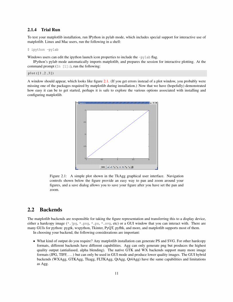
2.1.4 Trial RunTo test your matplotlib installation, run IPython in pylab mode, which includes special support for interactive use ofmatplotlib. Linux and Mac users, run the following in a shell:

$ ipython -pylab

Windows users can edit the ipython launch icon properties to include the -pylab flag.IPython’s pylab mode automatically imports matplotlib, and prepares the session for interactive plotting. At the

command prompt (In [1]:), run the following:

p l o t ( [ 1 , 2 , 3 ] )

A window should appear, which looks like figure 2.1. (If you get errors instead of a plot window, you probably weremissing one of the packages required by matplotlib during installation.) Now that we have (hopefully) demonstratedhow easy it can be to get started, perhaps it is safe to explore the various options associated with installing andconfiguring matplotlib.

Figure 2.1: A simple plot shown in the TkAgg graphical user interface. Navigationcontrols shown below the figure provide an easy way to pan and zoom around yourfigures, and a save dialog allows you to save your figure after you have set the pan andzoom.

2.2 BackendsThe matplotlib backends are responsible for taking the figure representation and transferring this to a display device,either a hardcopy image (*.jpg, *.png, *.ps, *.svg, etc) or a GUI window that you can interact with. There aremany GUIs for python: pygtk, wxpython, Tkinter, PyQT, pyfltk, and more, and matplotlib supports most of them.

In choosing your backend, the following considerations are important:

• What kind of output do you require? Any matplotlib installation can generate PS and SVG. For other hardcopyformats, different backends have different capabilities. Agg can only generate png but produces the highestquality output (antialiased, alpha blending). The native GTK and WX backends support many more imageformats (JPG, TIFF, . . . ) but can only be used in GUI mode and produce lower quality images. The GUI hybridbackends (WXAgg, GTKAgg, Tkagg, FLTKAgg, QtAgg, Qt4Agg) have the same capabilities and limitationsas Agg.

11

• Do you want to produce plots interactively from the python shell? Most GUIs have a mainloop and becomeunresponsive to outside input once they are launched. Thus you often need to use a custom shell to workinteractively with a GUI application from the shell (pycrust for wx, PyShell for gtk). A notable exception isTkinter, which can be controlled from a standard python shell or ipython. Fernando Perez, the author of ipython,has written a pylab mode for ipython that lets you use WX, GTK, Qt, Qt4 or Tk based backends interactivelyfrom the python shell. If you want to work interactively with matplotlib, the recommended approach is to useipython.

• What platform do you use most frequently? Do you want to embed matplotlib in an application that youdistribute across platforms? Do you need a GUI interface? Each of the python GUIs work on all major platforms,but some are easier than others to install. Each have different advantages: GTK is natural for linux and hasexcellent looking widgets but is a tough install on OS X. Tkinter is deployed with most python installationsbut has primitive looking widgets. wxpython has native widgets but can be difficult to install. Windows usersnote: the enthought edition of python from http://www.enthought.com/python comes with Tkinterand wxpython included. Now that Qt-4 has been released under the GPL for windows, the Qt backend is a newalternative with cross-platform compatibility.

• What features do you need? Some of the matplotlib features, including alpha blending, antialiasing, images andmathtext, are not ported to all backends. Agg and the *Agg hybrids support all matplotlib features (agg is a corematplotlib backend). Postscript, native GTK and native WX do not support alpha or antialiasing. SVG supportseverything except mathtext (which will hopefully be supported soon).

• Do you need dynamic images such as animation? The GUI backends vary in their ability to support rapidupdating of the image canvas. GTKAgg is currently the fastest backend for animation, with FLTKAgg a closesecond.

Once you have decided on which backends you want to use, make sure you have installed the required GUI toolkits(and devel versions if you are using a package manager). If you know you don’t want a particular backend or extension,you can set the appropriate flag to False in setup.py. Most users will want to keep the setup.py default BUILD_AGG =1. Exceptions to this are if you know you don’t need a GUI or you only want to produce vector graphics like postscript,svg or pdf. If you want to produce png output, keep BUILD_AGG = 1. Then install matplotlib and, if you have multiplebackends available to your matplotlib environment, edit your matplotlibrc files, as described in section 2.6, to selectyour default backend. Selecting your default backend may be important, especially if you intend to use matplotlib withan integrated development environment (IDE). This is described in the next section.

2.3 Integrated development environmentsIf you work primarily in an integrated development environment such as idle, pycrust, SciTE, or Pythonwin, youshould set your default backend to be compatible with the GUI your IDE uses. See Table 2.1 for a summary of thevarious python IDEs and their matplotlib compatibility.1

IDE GUI Backends and Optionsidle Tkinter Works best with TkAgg if idle is launched with the -n flagpycrust WX Works best with WX/WXAggpyshell GTK GTK/GTKAggScintilla and SciTE GTK Should work with GTK/GTKAgg backends but untestedEric3, Eric4 Qt, Qt4 works with QtAgg, Qt4Aggpythonwin MFC Unknown

Table 2.1: python IDEs and matplotlib compatibility.

1If you have experience with these or other IDEs and matplotlib backends to help me finish this table, please contact me or the matplotlib-develmailing list.

12

2.4 InteractiveThe recommended way to use matplotlib interactively from a shell is with IPython. IPython has a pylab mode(launched with ipython -pylab) that detects your matplotlibrc file and makes the right settings to run matplotlibwith your GUI of choice in interactive mode using threading. Ipython’s pylab mode is compatible with the Tk, GTK,WX and Qt GUI toolkits. GTK users will need to make sure that they have compiled GTK with threading for thisto work. Using ipython in pylab mode is basically a nobrainer because it knows enough about matplotlib internals tomake all the right settings for you.

peds−pc311 :~ > i p y t h o n −p y l a bPython 2 . 3 . 3 ( # 2 , Apr 13 2004 , 1 7 : 4 1 : 2 9 )Type "copyright" , "credits" or "license" f o r more i n f o r m a t i o n .

I P y t h o n 0 . 6 . 5 −− An enhanced I n t e r a c t i v e Python .? −> I n t r o d u c t i o n t o I P y t h o n ’s features.%magic -> Information about IPython’ s ’magic’ % f u n c t i o n s .h e l p −> Python ’s own help system.object? -> Details about ’ o b j e c t ’. ?object also works , ?? prints more.

Welcome to pylab , a matplotlib -based Python environment.help(matplotlib) -> generic matplotlib information.help(matlab) -> matlab -compatible commands from matplotlib.help(plotting) -> plotting commands.

In[1]: plot( rand(20), rand(20), ’go’ )

Note that you did not need to import any matplotlib names because in pylab mode ipython will import them foryou. ipython turns on interactive mode for you, and also provides a run command so you can run matplotlib scriptsfrom the matplotlib shell and then interactively update your figure. ipython will turn off interactive mode during a runcommand for efficiency, and then restore the interactive state at the end of the run.

>>> cd py thon / p r o j e c t s / m a t p l o t l i b / examples // home / j d h u n t e r / py thon / p r o j e c t s / m a t p l o t l i b / examples>>> run s i m p l e _ p l o t . py>>> t i t l e ( ’a new title’ , c o l o r =’r’ )

The pylab interface provides 4 commands that are useful for interactive control. Note again that the interactivesetting primarily controls whether the figure is redrawn with each plotting command. isinteractive returns theinteractive setting, ion turns interactive on, ioff turns it off, and draw forces a redraw of the entire figure. Thus whenworking with a big figure in which drawing is expensive, you may want to turn matplotlib’s interactive setting offtemporarily to avoid the performance hit

>>> run m y b i g f a t f i g u r e . py>>> i o f f ( ) # t u r n u p d a t e s o f f>>> t i t l e ( ’now how much would you pay?’ )>>> x t i c k l a b e l s ( f o n t s i z e =20 , c o l o r =’green’ )>>> draw ( ) # f o r c e a draw>>> s a v e f i g ( ’alldone’ , d p i =300)>>> c l o s e ( )>>> i o n ( ) # t u r n u p d a t e s back on>>> p l o t ( r and ( 2 0 ) , mfc=’g’ , mec=’r’ , ms=40 , mew=4 , l s =’--’ , lw =3)

If you are not using ipython -pylab, then by default, matplotlib defers drawing until the end of the script becausedrawing can be an expensive operation. Often you don’t want to update the plot every time a single property is changed,only once after all the properties have changed. But in interactive mode, eg from the standard python shell, you usuallydo want to update the plot with every command, eg, after changing the xlabel or the marker style of a line. To do this,you need to set interactive : True in your configuration file; see Section 2.6.

13

There are many python shells out there: the standard python shell, ipython, PyShell, pysh, pycrust. Some of theseare GUI dependent (PyShell/pycrust) and some are not (ipython, pysh). As discussed in backends Section 2.3, notall shells are compatible with all matplotlib backends because of GUI mainloop issues. With a non-GUI python shellsuch as the standard python shell or pysh, the TkAgg backend is the best choice for interactive use. Just set backend: TkAgg and interactive : True in your matplotlibrc file and fire up python. Then

# u s i n g m a t p l o t l i b i n t e r a c t i v e l y from t h e py thon s h e l l>>> from p y l a b import ∗>>> p l o t ( [ 1 , 2 , 3 ] )>>> x l a b e l ( ’hi mom’ )

should work out of the box. Note, in batch mode, ie when making figures from scripts, interactive mode can be slowsince it redraws the figure with each command. So you may want to think carefully before making this the defaultbehavior.

2.5 NumerixNumeric is the original python module for efficiently processing arrays of numeric data. While highly optimized forperformance and very stable, some limitations in the design made it inefficient for very large arrays, and developersdecided it was better to start with a new array package to solve some of these design problems. Thus numarray wasborn. In a sense, this caused the numerical python community to split into Numeric and numarray user groups. Toresolve this split, Travis Oliphant, one of the maintainers of Numeric, began work on a third package, based on theNumeric code base, which incorporated the advances made in numarray. This project is now called NumPy. NumPyis the successor to both Numeric and numarray, and is intended to reunite the numerical python community. An arrayinterface was developed in order to allow the three array packages to play well together and to easy migration toNumPy. Numeric is no longer undergoing active development, and the numarray release notes suggest users to switchto Numpy.

Matplotlib requires one of Numeric, numarray, or NumPy to operate. If you have no experience with any of thesepackages, you are strongly advised to install Numpy and read through some of the documentation before continuing.Since the array packages all play well together, we expect that in the near future, matplotlib will depend on NumPyalone. Until then, the matplotlib.numerix module, written by Todd Miller, allows you to choose between Numeric,numarray and NumPy at the prompt or in a config file. Thus when you do

# i m p o r t m a t p l o t l i b and a l l t h e numer ix f u n c t i o n sfrom p y l a b import ∗

you’ll not only get all the matplotlib pylab interface commands, but most of the Numeric, numarray or NumPy packageas well (depending on your numerix setting). All of the array creation and manipulation functions are imported,such as array, arange, take, where, etc. The other modules, such as mlab, fft and linear_algebra, are availableunder the numarray package structure. To make your matplotlib scripts as portable as possible with respect to yourchoice of array packages, it is advised not to explicitly import Numeric, numarray or NumPy. Rather, you should usematplotlib.numerix where possible, either by using the functions imported by pylab, or by explicitly importing thenumerix module, as in

# c r e a t e a numer ix namespaceimport m a t p l o t l i b . numer ix as nx = n . a r a n g e ( 1 0 0 )y = n . t a k e ( x , r a n g e ( 1 0 , 2 0 ) )

For the remainder of this manual, the term numerix is used to mean either the Numeric, numarray or NumPypackage.

2.5.1 Choosing Numeric, numarray, or NumPyTo select Numeric, numarray, or NumPy from the prompt, run your matplotlib script with

14

> python myscript.py --numarray # use numarray> python myscript.py --Numeric # use Numeric> python myscript.py --numpy # use NumPy

Typically, however, users will choose one option and make this setting in their rc file using either numerix : Numeric,numerix : numarray, or numerix : numpy; see Section 2.6.

2.6 Customization using matplotlibrc

Almost all of the matplotlib settings and figure properties can be customized with a plain text file matplotlibrc.This file is installed with the rest of the matplotlib data (fonts, icons, etc) into a directory determined by python’sinstallation module. Before compiling matplotlib, matplotlibrc resides in the same dir as setup.py and will becopied into your install path. Typical locations for this file are

C:\Python24\Lib\site-packages\matplotlib\mpl-data\matplotlibrc # windows/usr/lib/python2.4/site-packages/matplotlib/mpl-data/matplotlibrc # linux and friends

By default, the installer will overwrite the existing file in the install path, so if you want to preserve your changes,please move it to the .matplotlib directory in your HOME directory (and set the HOME environment variable ifnecessary).

In the rc file, you can set your backend (Section 2.2), your numerix setting (Section 2.5), whether you’ll be workinginteractively (Section 2.4) and default values for most of the figure properties.

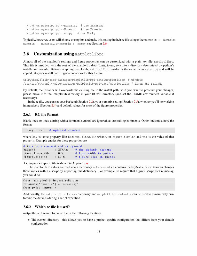
2.6.1 RC file formatBlank lines, or lines starting with a comment symbol, are ignored, as are trailing comments. Other lines must have theformat

key : v a l # o p t i o n a l comment

where key is some property like backend, lines.linewidth, or figure.figsize and val is the value of thatproperty. Example entries for these properties are

# t h i s i s a comment and i s i g n o r e dbackend : GTKAgg # t h e d e f a u l t backendl i n e s . l i n e w i d t h : 0 . 5 # l i n e wid th i n p o i n t sf i g u r e . f i g s i z e : 8 , 6 # f i g u r e s i z e i n i n c h e s

A complete sample rc file is shown in Appendix A.The matplotlib rc values are read into a dictionary rcParams which contains the key/value pairs. You can changes

these values within a script by importing this dictionary. For example, to require that a given script uses numarray,you could do

from m a t p l o t l i b import r cPa ramsrcParams [ ’numerix’ ] = ’numarray’from p y l a b import ∗

Additionally, the matplotlib.rcParams dictionary and matplotlib.rcdefaults can be used to dynamically cus-tomize the defaults during a script execution.

2.6.2 Which rc file is used?matplotlib will search for an rc file in the following locations

• The current directory - this allows you to have a project specific configuration that differs from your defaultconfiguration

15

• Your HOME dir. On linux and other UNIX operating systems, this environment variable is set by default.Windows users can set in the My Computer properties

• PATH/matplotlibrc where PATH is the return value of matplotlib.get_data_path(). This function lookswhere distutils would have installed the file - if it doesn’t find it there, it checks for the environment variableMATPLOTLIBDATA and uses that if found. The latter should be set if you are installing matplotlib to a non-standard location. Eg, if you install matplotlib with python setup.py build -prefix=/home/jdhunterthen set matplotlib data to /home/jdhunter/share/matplotlib.

• After all that, if it cannot find your rc file, it will issue a warning and use defaults. This is not recommended!

2.6.3 In the event of a problemmatplotlib uses a verbose setting, defined in the matplotlibrc file to determine how much information to report.

verbose.level : error # one of silent, error, helpful, debug, debug-annoyingverbose.fileo : sys.stdout # a log filename, sys.stdout or sys.stderrverbose.erro : sys.stderr # a log filename, sys.stdout or sys.stderr

These settings control how much information matplotlib gives you at runtime and where it goes. The verbosity levelsare: silent, error, helpful, debug, debug-annoying. At the error level, you will only get error messages.Any level is inclusive of all the levels below it. Ie, if your setting is helpful, you’ll also get all the error messages.If you setting is debug, you’ll get all the error and helpful messages. It is not recommended to make your settingsilent because you will not even get error messages. You can access the verbose instance in your code frommatplotlib import verbose.

The verbose.fileo setting gives the destination for any calls to the verbose report function. The verbose.errosetting gives the destination for any calls to verbose error reporting function. These objects can a filename or a fullpath to a filename, sys.stderr, or sys.stdout. You can override the rc default verbosity from the command line bygiving the flags -verbose-LEVEL where LEVEL is one of the legal levels, eg -verbose-error -verbose-helpful.

If you run into a problem and want to ask for help or report a bug to the mailing-list, please set verbose to helpfulor debug and paste the output into your report. Also, please include the shortest possible example code that reproducesthe problem. With the example code and verbose output, other readers of the mailing list have a much better chance ofunderstanding the problem and offering a solution. The email address is matplotlib-users@lists.sourceforge.net.Finally, for those who are using the development sources from the sourceforge subversion repository, please reportproblems to matplotlib-devel@lists.sourceforge.net instead of matplotlib-users@lists.sourceforge.net.You can subscribe to either mailing list at http://sourceforge.net/mail/?group_id=80706.

16

Chapter 3

The pylab interface

Although matplotlib has a full object oriented API (see Chapter 8), the primary way people create plots is via the pylabinterface, which can be imported with

from p y l a b import ∗

This import command brings in all of the matplotlib code needed to produce plots, the extra MATLABTM compati-ble, non-plotting functions found in matplotlib.mlab and all of the matplotlib.numerix code needed to create andmanipulate arrays. When you import pylab, you will get all of NumPy (or Numeric or numarray depending on yournumerix setting).

matplotlib is organized around figures and axes. The figure contains an arbitrary number of axes, which can beplaced anywhere in the figure you want, including over other axes. You can directly create and manage your ownfigures and axes, but if you don’t, matplotlib will try and do the right thing by automatically creating default figuresand axes for you.

There are two ways of working in the pylab interface: interactively or in script mode. When working interactively,you want every plotting command to update the figure. Under the hood, this means that the canvas is redrawn afterevery command that affects the figure. When working in script mode, this is inefficient. In this case, you only wantthe figure to be drawn once, either to the GUI window or saved to a file. To handle these two cases, matplotlibhas an interactive setting in matplotlibrc. When interactive : True, the figure will be redrawn with eachcommand. When interactive : False, the figure will be drawn only when there is a call to show or savefig.In the examples that follow, I’ll assume you have set interactive : True in your matplotlibrc file and areworking from an interactive python shell using a compatible backend. Please make sure you have read and understoodSections 2.2, 2.3, 2.4 and 2.6, before trying these examples.

3.1 Simple plotsJust about the simplest plot you can create is

>>> from p y l a b import ∗>>> p l o t ( [ 1 , 2 , 3 ] )

I have set my backend to backend : TkAgg, which causes the plot in Figure 2.1 to appear, with navigation controlsfor interactive panning and zooming.

I can continue to decorate the plot with labels and titles

>>> x l a b e l ( ’time (s)’ )>>> y l a b e l ( ’volts’ )>>> t i t l e ( ’A really simple plot’ )>>> g r i d ( True )

17

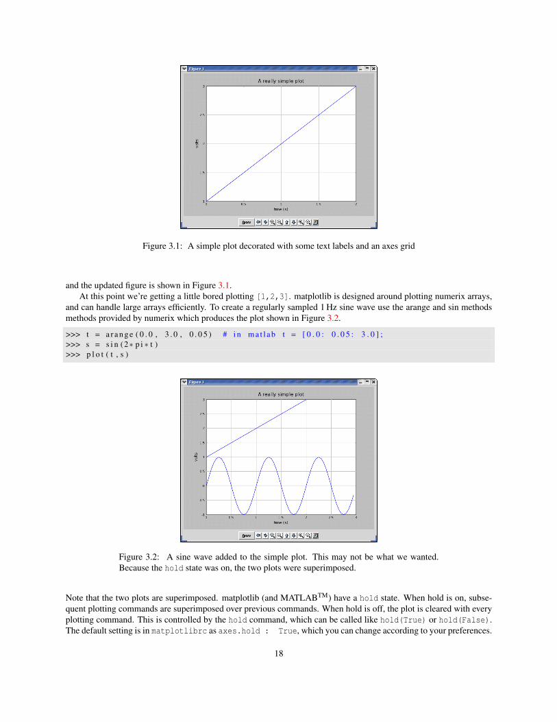
Figure 3.1: A simple plot decorated with some text labels and an axes grid

and the updated figure is shown in Figure 3.1.At this point we’re getting a little bored plotting [1,2,3]. matplotlib is designed around plotting numerix arrays,

and can handle large arrays efficiently. To create a regularly sampled 1 Hz sine wave use the arange and sin methodsmethods provided by numerix which produces the plot shown in Figure 3.2.

>>> t = a r a n g e ( 0 . 0 , 3 . 0 , 0 . 0 5 ) # i n ma t l ab t = [ 0 . 0 : 0 . 0 5 : 3 . 0 ] ;>>> s = s i n (2∗ p i ∗ t )>>> p l o t ( t , s )

Figure 3.2: A sine wave added to the simple plot. This may not be what we wanted.Because the hold state was on, the two plots were superimposed.

Note that the two plots are superimposed. matplotlib (and MATLABTM) have a hold state. When hold is on, subse-quent plotting commands are superimposed over previous commands. When hold is off, the plot is cleared with everyplotting command. This is controlled by the hold command, which can be called like hold(True) or hold(False).The default setting is in matplotlibrc as axes.hold : True, which you can change according to your preferences.

18

To clear the previous plot and reissue the plot command for just the sine wave, you can use cla to clear the currentaxes and clf to clear the current figure, or simply turn the hold state off.

>>> ho ld ( F a l s e )>>> p l o t ( t , s )

3.2 More on plot

3.2.1 Multiple linesplot is a versatile command, and will create an arbitrary number of lines with different line styles and markers. Thisexample plots a sine wave and a damped exponential using the default line styles

>>> c l f ( ) # c l e a r t h e f i g u r e>>> t = a r a n g e ( 0 . 0 , 5 . 0 , 0 . 0 5 )>>> s1 = s i n (2∗ p i ∗ t )>>> s2 = s1 ∗ exp(− t )>>> p l o t ( t , s1 , t , s2 )

If you plot multiple lines in a single plot command, the line color will cycle through a list of predefined colors. Thedefault line color and line style are determined by the rc parameters lines.style and lines.color. You can includean optional third string argument to each line in the plot command, which specifies any of the line style, marker styleand line color. To plot the above using a green dashed line with circle markers, and a red dotted line with circlemarkers, as shown in Figure 3.3,

>>> c l f ( )>>> p l o t ( t , s1 , ’g--o’ , t , s2 , ’r:s’ )>>> l e g e n d ( ( ’sine wave’ , ’damped exponential’ ) )

Figure 3.3: All line plots take an optional third string argument, which is composed of(optionally) a line color (eg, ’r’, ’g’, ’k’), a line style (eg, ’-’, ’–’, ’:’) and a line marker(’o’, ’s’, ’d’). The sine wave line (green dashed line with circle markers) is created with’g–o’. The legend command will automatically create a legend for all the lines in theplot.

The color part of the format string applies only to the facecolor of 2D plot markers like circles, triangles, and squares.The edgecolor of these markers will be determined by the default rc parameter lines.markeredgecolor and can bedefined for individual lines using the methods discussed below.

19

3.2.2 Controlling line propertiesIn the last section, we showed how to choose the default line properties using plot format strings. For finer grainedcontrol, you can set any of the attributes of a matplotlib.lines.Line2D instance. There are three ways to do this:using keyword arguments, calling the line methods directly, or using the set command. The line properties are shownin Table 3.1.

Property Valuealpha The alpha transparency on 0-1 scaleantialiased True or False - use antialised renderingcolor A matplotlib color argdata_clipping Whether to use numeric to clip datalabel A string optionally used for legendlinestyle One of - : -. -linewidth A float, the line width in pointsmarker One of + , o . s v x > <, etcmarkeredgewidth The line width around the marker symbolmarkeredgecolor The edge color if a marker is usedmarkerfacecolor The face color if a marker is usedmarkersize The size of the marker in points

Table 3.1: Line properties; see pylab.plot for more marker styles

Using keyword arguments to control line properties

You can set any of the line properties listed in Table 3.1 using keyword arguments to the plot command. The followingcommand plots large green diamonds with a red border

>>> p l o t ( t , s1 , m a r k e r s i z e =15 , marker =’d’ , \. . . m a r k e r f a c e c o l o r =’g’ , m a r k e r e d g e c o l o r =’r’ )

Using set to control line properties

You can set any of the line properties listed in Table 3.1 using the set command. Set operates on the return value ofthe plot command (a list of lines), so you need to save the lines. You can use an arbitrary number of key/value pairs

>>> l i n e s = p l o t ( t , s1 )>>> s e t ( l i n e s , m a r k e r s i z e =15 , marker =’d’ , \. . . m a r k e r f a c e c o l o r =’g’ , m a r k e r e d g e c o l o r =’r’ )

set can either operate on a single instance or a sequence of instances (in the example code above, lines is a lengthone sequence of lines). Under the hood, if you pass a keyword arg named something, set looks for a method ofthe object called set_something and will call it with the value you pass. If set_something does not exist, then anexception will be raised.

Using matplotlib.lines.Line2D methods

You can also call Line2D methods directly. The return value of plot is a sequence of matplotlib.lines.Line2Dinstances. Note in the example below, I use tuple unpacking with the “,” to extract the first element of the sequence asline: line, = plot(t, s1)

>>> l i n e , = p l o t ( t , s1 )>>> l i n e . s e t _ m a r k e r s i z e ( 1 5 )>>> l i n e . s e t _ m a r k e r ( ’d’ )

20

>>> l i n e . s e t _ m a r k e r f a c e c o l o r ( ’g’ )>>> l i n e . s e t _ m a r k e r e d g e c o l o r ( ’r’ )

Note, however, that we haven’t issued any pylab commands after the initial plot command so the figure will not beredrawn even though interactive mode is set. To trigger a redraw, you can simply resize the figure window a little orcall the draw method. The fruits of your labors are shown in Figure 3.4.

>>> draw ( )

Figure 3.4: Large green diamonds with red borders, created with three different recipes.

Abbreviated method names

Abbreviation Fullnameaa antialiasedc colorls linestylelw linewidthmec markeredgecolormew markeredgewidthmfc markerfacecolorms markersize

Table 3.2: Abbreviated names for line properties. You can use any of the line customiza-tion methods above with abbreviated names.

When working from an interactive python shell, typing ’markerfacecolor’ can be a pain – too many keystrokes.The matplotlib.lines.Line2D class provides a number of abbreviated method names, listed in Table 3.2.Thus you can, for example, call

# no a n t i a l i a s i n g , t h i c k g r e e n markeredge l i n e s>>> p l o t ( r a n g e ( 1 0 ) , ’ro’ , aa= F a l s e , mew=2 , mec=’g’ )

21

3.3 Color argumentsmatplotlib is fairly tolerant of a number of formats for passing color information. As discussed above, you can use andof the single character color strings listed in Table 3.3. Additionally, anywhere a color character string is accepted,you can also use a grayscale, hex, RGB color argument, or any legal hml color name, ebg “red” or “darkslategray”.

Figure 3.5: Lots of different ways to specify colors generated from Listing 3.1– notnecessarily recommended for aesthetic quality!

Listing 3.1: Wild and wonderful ways to specify colors; see Figure 3.5from p y l a b import ∗

# a x i s background i n da rk s l a t e g rays u b p l o t ( 1 1 1 , a x i s b g = ( 0 . 1 8 4 3 , 0 . 3 0 9 8 , 0 . 3 0 9 8 ) )t = a r a n g e ( 0 . 0 , 1 . 0 , 0 . 0 1 )s = s i n (2∗2∗ p i ∗ t )

# ye l l ow c i r c l e s wi th r e d edge c o l o rp l o t ( t , s , ’yo’ , m a r k e r e d g e c o l o r =’r’ )x l a b e l ( ’time (s)’ , c o l o r =’b’ ) # x l a b e l i s b l u ey l a b e l ( ’voltage (mV)’ , c o l o r =’0.5’ ) # y l a b e l i s l i g h t g r ayt i t l e ( "Don’t try this at home , folks" , c o l o r =’#afeeee’ )

3.4 Loading and saving datapylab provides support for loading and saving ASCII arrays or vectors with the load and save command. matplotlib.numerixprovides support for loading and saving binary arrays with the fromstring and tostring methods.

3.4.1 Loading and saving ASCII dataSuppose you have an ASCII file of measured times and voltages like so

22

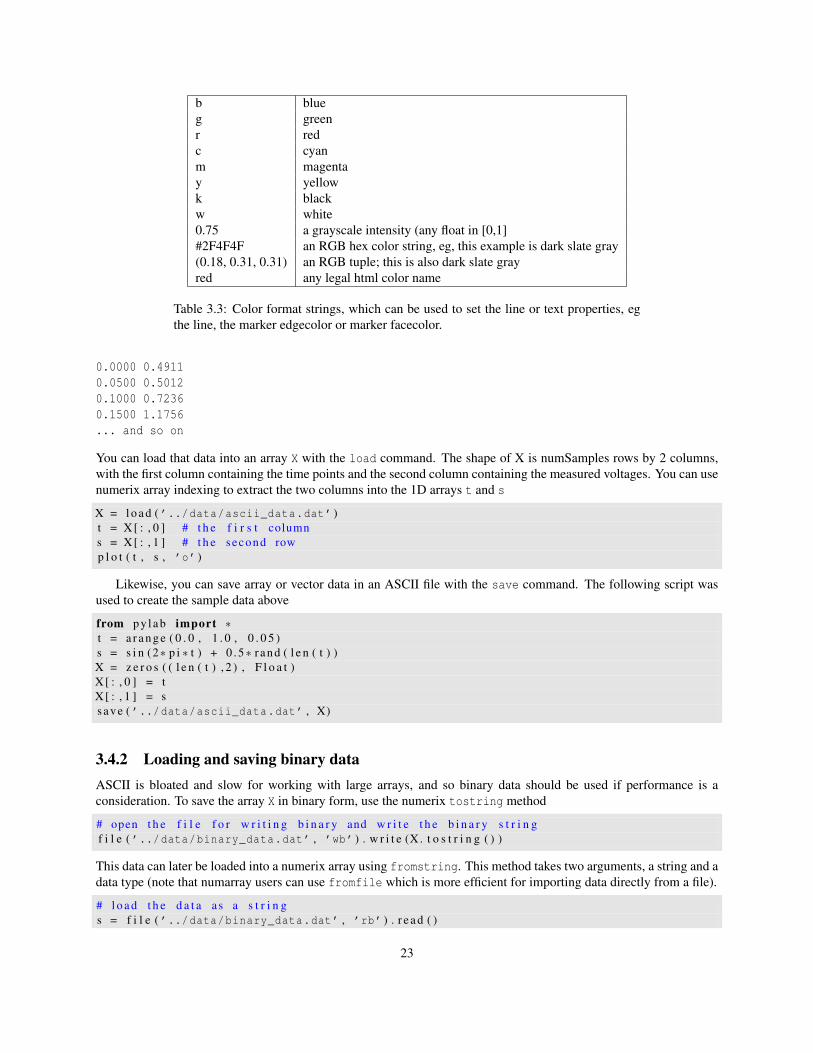
b blueg greenr redc cyanm magentay yellowk blackw white0.75 a grayscale intensity (any float in [0,1]#2F4F4F an RGB hex color string, eg, this example is dark slate gray(0.18, 0.31, 0.31) an RGB tuple; this is also dark slate grayred any legal html color name

Table 3.3: Color format strings, which can be used to set the line or text properties, egthe line, the marker edgecolor or marker facecolor.

0.0000 0.49110.0500 0.50120.1000 0.72360.1500 1.1756... and so on

You can load that data into an array X with the load command. The shape of X is numSamples rows by 2 columns,with the first column containing the time points and the second column containing the measured voltages. You can usenumerix array indexing to extract the two columns into the 1D arrays t and s

X = l o a d ( ’../data/ascii_data.dat’ )t = X [ : , 0 ] # t h e f i r s t columns = X[ : , 1 ] # t h e second rowp l o t ( t , s , ’o’ )

Likewise, you can save array or vector data in an ASCII file with the save command. The following script wasused to create the sample data above

from p y l a b import ∗t = a r a n g e ( 0 . 0 , 1 . 0 , 0 . 0 5 )s = s i n (2∗ p i ∗ t ) + 0 . 5∗ r and ( l e n ( t ) )X = z e r o s ( ( l e n ( t ) , 2 ) , F l o a t )X [ : , 0 ] = tX [ : , 1 ] = ssave ( ’../data/ascii_data.dat’ , X)

3.4.2 Loading and saving binary dataASCII is bloated and slow for working with large arrays, and so binary data should be used if performance is aconsideration. To save the array X in binary form, use the numerix tostring method

# open t h e f i l e f o r w r i t i n g b i n a r y and w r i t e t h e b i n a r y s t r i n gf i l e ( ’../data/binary_data.dat’ , ’wb’ ) . w r i t e (X. t o s t r i n g ( ) )

This data can later be loaded into a numerix array using fromstring. This method takes two arguments, a string and adata type (note that numarray users can use fromfile which is more efficient for importing data directly from a file).

# l o a d t h e d a t a as a s t r i n gs = f i l e ( ’../data/binary_data.dat’ , ’rb’ ) . r e a d ( )

23

# c o n v e r t t o 1D numer ix a r r a y o f t y p e F l o a tX = f r o m s t r i n g ( s , F l o a t )

# r e s h a p e t o numSamples rows by 2 columnsX. shape = l e n (X) / 2 , 2t = X [ : , 0 ] # t h e f i r s t columns = X[ : , 1 ] # t h e second rowp l o t ( t , s , ’o’ )

Note that although Numerix and numarray use different typecode arguments (Numeric uses strings whereas numarrayuses type objects), the matplotlib.numerix compatibility layer provides symbols which will work with either numerixrc setting.

3.4.3 Processing several data filesSince python is a programming language par excellence, it is easy to process data in batch. When I started the grad-ual transition from a full time MATLABTM user to a full time python user, I began processing my data in pythonand saving the results to data files for plotting in MATLABTM. When that became too cumbersome, I decided towrite matplotlib so I could have all the functionality I needed in one environment. Here is a brief example show-ing how to iterate over several data files, named basename001.dat, basename002.dat, basename003.dat, ...basename100.dat and plot all of the traces to the same axes. I’ll assume for this example that each file is a 1D ASCIIarray, which I can load with the load command.

ho ld ( True ) # s e t t h e ho ld s t a t e t o be onf o r i in r a n g e ( 1 , 1 0 1 ) : # s t a r t a t 1 , end a t 100

fname = ’basename%03d.dat’%i # %03d pads t h e i n t e g e r s wi th z e r o sx = l o a d ( fname )p l o t ( x )

3.5 axes and figuresAll the examples thus far used implicit figure and axes creation. You can use the functions figure, subplot, and axesto explicitly control this process. Let’s take a look at what happens under the hood when you issue the commands

>>> from p y l a b import ∗>>> p l o t ( [ 1 , 2 , 3 ] )

When plot is called, the pylab interface makes a call to gca() (“get current axes”) to get a reference to the currentaxes. gca in turn, makes a call to gcf to get a reference to the current figure. gcf, finding that no figure has beencreated, creates the default figure figure() and returns it. gca will then return the current axes of that figure if itexists, or create the default axes subplot(111) if it does not. Thus the code above is equivalent to

>>> from p y l a b import ∗>>> f i g u r e ( )>>> s u b p l o t ( 1 1 1 )>>> p l o t ( [ 1 , 2 , 3 ] )

3.5.1 figure

You can create and manage an arbitrary number of figures using the figure command. The standard way to create afigure is to number them from 1 . . .N. A call to figure(1) creates figure 1 if it does not exist, makes figure 1 active(gcf will return a reference to it), and returns the matplotlib.figure.Figure instance. The syntax of the figurecommand is

24

def f i g u r e ( num=1 ,f i g s i z e = None , # d e f a u l t s t o r c f i g u r e . f i g s i z ed p i = None , # d e f a u l t s t o r c f i g u r e . d p if a c e c o l o r = None , # d e f a u l t s t o r c f i g u r e . f a c e c o l o re d g e c o l o r = None , # d e f a u l t s t o r c f i g u r e . e d g e c o l o rf rameon = True , # whe the r t o draw t h e f i g u r e f rame) :

figsize gives the figure size in inches and is width by height. Eg, to create a figure 12 inches wide and 2 inches high,you can call figure(figsize=(12,2)). dpi gives the dots per inch of your display device. Increasing this numbereffectively creates a higher resolution figure. facecolor and edgecolor determine the face and edge color of the figurerectangular background. This is what gives the figure a gray background in the GUI figures such as Figure 2.1. Youcan turn this background completely off by setting frameon=False. The default for saving figures is to have a whiteface and edge color, and all of these properties can be customized using the rc parameters figure.* and savefig.*.

In typical usage, you will only provide the figure number, and let your rc parameters govern the other figureattributes

>>> f i g u r e ( 1 )>>> p l o t ( [ 1 , 2 , 3 ] )>>> f i g u r e ( 2 )>>> p l o t ( [ 4 , 5 , 6 ] )>>> t i t l e ( ’big numbers’ ) # f i g u r e 2 t i t l e>>> f i g u r e ( 1 )>>> t i t l e ( ’small numbers’ ) # f i g u r e 1 t i t l e

You can close a figure simply by clicking on the close “x” in the GUI window, or by issuing the close command.close can be used to close the current figure, a figure referenced by number, a given figure instance, or all figures

• close() by itself closes the current figure

• close(num) closes figure number num

• close(fig) where fig is a figure instance closes that figure

• close(’all’) closes all the figure windows

If you close a figure directly, eg close(2) the previous current figure is restored to the current figure. clf is used toclear the current figure without closing it.

If you save the return value of the figure command, you can call any of the methods provided by matplotlib.figure.Figure,for example, you can set the figure facecolor

>>> f i g = f i g u r e ( 1 )>>> f i g . s e t _ f a c e c o l o r ( ’g’ )

or use set for the same purpose

>>> s e t ( f i g , f a c e c o l o r =’g’ )

3.5.2 subplot

axes and subplot are both used to create axes in a figure. subplot is used more commonly, and creates axes assuminga regular grid of axes numRows by numCols. For example, to create two rows and one column of axes, you would usesubplot(211) to create the upper axes and subplot(212) to create the lower axes. The last digit counts across therows.

25

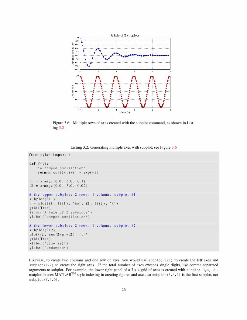
Figure 3.6: Multiple rows of axes created with the subplot command, as shown in List-ing 3.2

Listing 3.2: Generating multiple axes with subplot; see Figure 3.6

from p y l a b import ∗

def f ( t ) :’a damped oscillation’re turn cos (2∗ p i ∗ t ) ∗ exp(− t )

t 1 = a r a n g e ( 0 . 0 , 5 . 0 , 0 . 1 )t 2 = a r a n g e ( 0 . 0 , 5 . 0 , 0 . 0 2 )

# t h e upper s u b p l o t ; 2 rows , 1 column , s u b p l o t #1s u b p l o t ( 2 1 1 )l = p l o t ( t1 , f ( t 1 ) , ’bo’ , t2 , f ( t 2 ) , ’k’ )g r i d ( True )t i t l e ( ’A tale of 2 subplots’ )y l a b e l ( ’Damped oscillation’ )

# t h e lower s u b p l o t ; 2 rows , 1 column , s u b p l o t #2s u b p l o t ( 2 1 2 )p l o t ( t2 , cos (2∗ p i ∗ t 2 ) , ’r>’ )g r i d ( True )x l a b e l ( ’time (s)’ )y l a b e l ( ’Undamped’ )

Likewise, to create two columns and one row of axes, you would use subplot(121) to create the left axes andsubplot(122) to create the right axes. If the total number of axes exceeds single digits, use comma separatedarguments to subplot. For example, the lower right panel of a 3 x 4 grid of axes is created with subplot(3,4,12).matplotlib uses MATLABTM style indexing in creating figures and axes, so subplot(3,4,1) is the first subplot, notsubplot(3,4,0).

26

The subplot command returns a matplotlib.axes.Subplot instance, which is derived from matplotlib.axes.Axes.Thus you can call and Axes or Subplot method on it. When creating multiple subplots with the same axes, for examplethe same time axes, sometimes it helps to turn off the x tick labeling for all but the lowest plot. Here is some examplecode

s u b p l o t ( 2 1 1 )p l o t ( [ 1 , 2 , 3 ] , [ 1 , 2 , 3 ] )s e t ( gca ( ) , x t i c k l a b e l s = [ ] )

s u b p l o t ( 2 1 2 )p l o t ( [ 1 , 2 , 3 ] , [ 1 , 4 , 9 ] )

Likewise, with multiple columns and shared y axes, you may want turn off the ytick labels for all but the first row.The subplot command returns a matplotlib.axes.Subplot instance, which is derived from matplotlib.axes.Axes.Thus you can call and Axes or Subplot method on it. Subplot defines some helper methods (is_first_row, is_first_col,is_last_row, is_last_col, to help you conditionally set subplot properties, eg

c n t = 0f o r i in r a n g e ( numRows ) :

f o r j in r a n g e ( numCols ) :c n t += 1ax = s u b p l o t ( numRows , numCols , c n t )p l o t ( b lah , b l a h )i f ax . i s _ l a s t _ r o w ( ) : x l a b e l ( ’time (s)’ )i f ax . i s _ f i r s t _ c o l ( ) : y l a b e l ( ’volts’ )

Here is some example code to create multiple figures and axes, using the figure and subplot command to controlthe current figure and axes.

from p y l a b import ∗

t = a r a n g e ( 0 . 0 , 2 . 0 , 0 . 0 1 )s1 = s i n (2∗ p i ∗ t )s2 = s i n (4∗ p i ∗ t )

f i g u r e ( 1 )s u b p l o t ( 2 1 1 )p l o t ( t , s1 )s u b p l o t ( 2 1 2 )p l o t ( t , 2∗ s1 )

f i g u r e ( 2 )p l o t ( t , s2 )

# now s w i t c h back t o f i g u r e 1 and make some changes t o t h e upper# s u b p l o tf i g u r e ( 1 )s u b p l o t ( 2 1 1 )p l o t ( t , s2 , ’gs’ )s e t ( gca ( ) , ’xticklabels’ , [ ] )

show ( )

3.5.3 axes

When you need a finer grained control over axes placement than afforded by subplot, use the axes command.The axes command in initialized with a rectangle [left, bottom, width, height] in relative figure coordinates.

27

left, bottom = (0, 0) is the bottom left of the of the figure canvas, and a width/height of 1 spans the figurewidth/height. This to create an axes that entirely fills the figure canvas, you would do axes([0, 1, 0, 1]). Thismay not be a good idea, because it leaves no room for text labels. axes([0.25, 0.25, 0.5, 0.5]) creates an axesoffset by one quarter of the figure width and height on all sides.

There are several ways to use the axes command; in all cases, a matplotlib.axes.Axes instance is returned

• axes() by itself creates a default full subplot(111) window axis

• axes(rect, axisbg=’w’) where rect=[left, bottom, width, height] in normalized (0,1) units. axisbgis the background color for the axis, default white.

• axes(ax) where ax is an axes instance makes ax current.

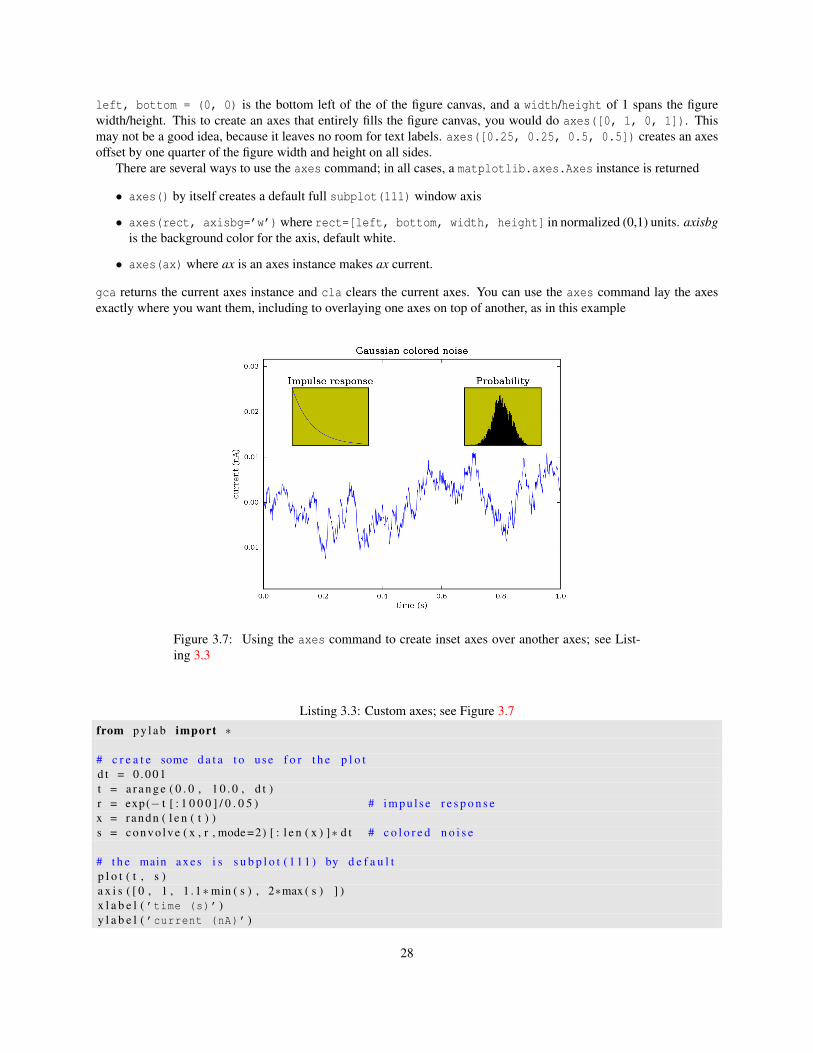
gca returns the current axes instance and cla clears the current axes. You can use the axes command lay the axesexactly where you want them, including to overlaying one axes on top of another, as in this example

Figure 3.7: Using the axes command to create inset axes over another axes; see List-ing 3.3

Listing 3.3: Custom axes; see Figure 3.7from p y l a b import ∗

# c r e a t e some d a t a t o use f o r t h e p l o td t = 0 .001t = a r a n g e ( 0 . 0 , 1 0 . 0 , d t )r = exp(− t [ : 1 0 0 0 ] / 0 . 0 5 ) # i m p u l s e r e s p o n s ex = randn ( l e n ( t ) )s = c o n v o l v e ( x , r , mode =2) [ : l e n ( x ) ]∗ d t # c o l o r e d n o i s e

# t h e main axes i s s u b p l o t ( 1 1 1 ) by d e f a u l tp l o t ( t , s )a x i s ( [ 0 , 1 , 1 . 1∗min ( s ) , 2∗max ( s ) ] )x l a b e l ( ’time (s)’ )y l a b e l ( ’current (nA)’ )

28

t i t l e ( ’Gaussian colored noise’ )

# t h i s i s an i n s e t axes ove r t h e main axesa = axes ( [ . 6 5 , . 6 , . 2 , . 2 ] , a x i s b g =’y’ )n , b in s , p a t c h e s = h i s t ( s , 400 , normed =1)t i t l e ( ’Probability’ )s e t p ( a , x t i c k s = [ ] , y t i c k s = [ ] )

# t h i s i s a n o t h e r i n s e t axes ove r t h e main axesa = axes ( [ 0 . 2 , 0 . 6 , . 2 , . 2 ] , a x i s b g =’y’ )p l o t ( t [ : l e n ( r ) ] , r )t i t l e ( ’Impulse response’ )s e t p ( a , x l im = ( 0 , . 2 ) , x t i c k s = [ ] , y t i c k s = [ ] )

3.6 Textmatplotlib has excellent text support, including newline separated text with arbitrary rotations and mathematical ex-pressions. freetype2 support produces very nice, antialiased fonts, that look good even at small raster sizes. It includesits own font_manager, thanks to Paul Barrett, which implements a cross platform, W3C compliant font finding algo-rithm. You have total control over every text property (font size, font weight, text location and color, etc) with sensibledefaults set in the rc file. And significantly for those interested in mathematical or scientific figures, matplotlib imple-ments a large number of TEX math symbols and commands, to support mathematical expressions anywhere in yourfigure. To get the most out of text in matplotlib, you should use a backend that supports freetype2 and mathtext,notably all the *Agg backends (see Section 2.2), or the postscript backend, which embeds the freetype fonts directlyinto the PS/EPS output file.

3.6.1 Basic text commandsThe following commands are used to create text in the pylab interface

• xlabel(s) - add a label s to the x axis

• ylabel(s) - add a label s to the y axis

• title(s) - add a title s to the axes

• text(x, y, s) - add text s to the axes at x, y in data coords

• figtext(x, y, s) - add text to the figure at x, y in relative 0-1 figure coords

3.6.2 Text propertiesThe text properties are listed in Table 3.4. As with lines, there are three ways to set text properties: using keywordarguments to a text command, calling set on a text instance or a sequence of text instances, or calling an instancemethod on a text instance. These three are illustrated below

# keyword a r g s>>> x l a b e l ( ’time (s)’ , c o l o r =’r’ , s i z e =16)>>> t i t l e ( ’Fun with text’ , h o r i z o n t a l a l i g n m e n t =’left’ )

# use s e t>>> l o c s , l a b e l s = x t i c k s ( )>>> s e t ( l a b e l s , c o l o r =g’, rotation=45)

29

# instance methods>>> l = ylabel(’ v o l t s ’)>>> l.set_weight(’ bo ld ’)

Property Valuealpha The alpha transparency on 0-1 scalecolor A matplotlib color argfamily set the font family, eg ’sans-serif’, ’cursive’, ’fantasy’fontangle the font slant, one of ’normal’, ’italic’, ’oblique’horizontalalignment ’left’, ’right’ or ’center’multialignment ’left’, ’right’ or ’center’ only for multiline stringsname the font name, eg, ’Sans’, ’Courier’, ’Helvetica’position the x,y locationvariant the font variant, eg ’normal’, ’small-caps’rotation the angle in degrees for rotated textsize the fontsize in points, eg, 8, 10, 12style the font style, one of ’normal’, ’italic’, ’oblique’text set the text string itselfverticalalignment ’top’, ’bottom’ or ’center’weight the font weight, eg ’normal’, ’bold’, ’heavy’, ’light’

Table 3.4: Properties of matplotlib.text.Text

See the example http://matplotlib.sourceforge.net/examples/fonts_demo_kw.py which makes extensiveuse of font properties for more information. See also Chapter 4 for more discussion of the font finder algorithm andthe meaning of these properties.

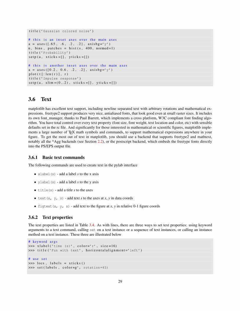
3.6.3 Text layoutYou can layout text with the alignment arguments horizontalalignment, verticalalignment, and multialignment. hor-izontalalignment controls whether the x positional argument for the text indicates the left, center or right side of thetext bounding box. verticalalignment controls whether the y positional argument for the text indicates the bottom,center or top side of the text bounding box. multialignment, for newline separated strings only, controls whether thedifferent lines are left, center or right justified. Here is an example which uses the text command to show the variousalignment possibilities. The use of transform=ax.transAxes throughout the code indicates that the coordinates aregiven relative to the axes bounding box, with 0,0 being the lower left of the axes and 1,1 the upper right.

Listing 3.4: Aligning text; see Figure 3.8from p y l a b import ∗from m a t p l o t l i b . p a t c h e s import R e c t a n g l e

# b u i l d a r e c t a n g l e i n axes c o o r d sl e f t , w id th = . 2 5 , . 5bottom , h e i g h t = . 2 5 , . 5r i g h t = l e f t + wid tht o p = bot tom + h e i g h tax = gca ( )p = R e c t a n g l e ( ( l e f t , bo t tom ) , width , h e i g h t ,

f i l l = F a l s e ,)

# axes c o o r d i n a t e s a r e 0 ,0 i s bot tom l e f t and 1 ,1 i s uppe r r i g h tp . s e t _ t r a n s f o r m ( ax . t r a n s A x e s )p . s e t _ c l i p _ o n ( F a l s e )

30

Figure 3.8: Aligning text with horizontalalignment, verticalalignment, and multialign-ment options to the text command; see Listing 3.4

ax . a d d _ p a t c h ( p )

ax . t e x t ( l e f t , bot tom , ’left top’ ,h o r i z o n t a l a l i g n m e n t =’left’ ,v e r t i c a l a l i g n m e n t =’top’ ,t r a n s f o r m =ax . t r a n s A x e s )

ax . t e x t ( l e f t , bot tom , ’left bottom’ ,h o r i z o n t a l a l i g n m e n t =’left’ ,v e r t i c a l a l i g n m e n t =’bottom’ ,t r a n s f o r m =ax . t r a n s A x e s )

ax . t e x t ( r i g h t , top , ’right bottom’ ,h o r i z o n t a l a l i g n m e n t =’right’ ,v e r t i c a l a l i g n m e n t =’bottom’ ,t r a n s f o r m =ax . t r a n s A x e s )

ax . t e x t ( r i g h t , top , ’right top’ ,h o r i z o n t a l a l i g n m e n t =’right’ ,v e r t i c a l a l i g n m e n t =’top’ ,

31

t r a n s f o r m =ax . t r a n s A x e s )

ax . t e x t ( r i g h t , bottom , ’center top’ ,h o r i z o n t a l a l i g n m e n t =’center’ ,v e r t i c a l a l i g n m e n t =’top’ ,t r a n s f o r m =ax . t r a n s A x e s )

ax . t e x t ( l e f t , 0 . 5 ∗ ( bot tom + t o p ) , ’right center’ ,h o r i z o n t a l a l i g n m e n t =’right’ ,v e r t i c a l a l i g n m e n t =’center’ ,r o t a t i o n =’vertical’ ,t r a n s f o r m =ax . t r a n s A x e s )

ax . t e x t ( l e f t , 0 . 5 ∗ ( bot tom + t o p ) , ’left center’ ,h o r i z o n t a l a l i g n m e n t =’left’ ,v e r t i c a l a l i g n m e n t =’center’ ,r o t a t i o n =’vertical’ ,t r a n s f o r m =ax . t r a n s A x e s )

ax . t e x t ( 0 . 5 ∗ ( l e f t + r i g h t ) , 0 . 5 ∗ ( bot tom + t o p ) , ’middle’ ,h o r i z o n t a l a l i g n m e n t =’center’ ,v e r t i c a l a l i g n m e n t =’center’ ,t r a n s f o r m =ax . t r a n s A x e s )

ax . t e x t ( r i g h t , 0 . 5 ∗ ( bot tom + t o p ) , ’centered’ ,h o r i z o n t a l a l i g n m e n t =’center’ ,v e r t i c a l a l i g n m e n t =’center’ ,r o t a t i o n =’vertical’ ,t r a n s f o r m =ax . t r a n s A x e s )

ax . t e x t ( l e f t , top , ’rotated\nwith newlines’ ,h o r i z o n t a l a l i g n m e n t =’center’ ,v e r t i c a l a l i g n m e n t =’center’ ,r o t a t i o n =45 ,t r a n s f o r m =ax . t r a n s A x e s )

a x i s ( ’off’ )

3.6.4 mathtextmatplotlib supports TEX mathematical expressions anywhere a text string can be used, as long as the string is delimitedby “$” on both sides, as in r′$5\lambda$′; embedded mathtext strings, such as in r′The answer is $5\lambda$′ arenot currently supported. A large set of the TEX symbols from the computer modern fonts are provided. Subscriptingand superscripting are supported, as well as the over/under style of subscripting with \sum, \int etc.

Note that matplotlib does not use or require that TEX be installed on your system, as it does not use it. Rather, it usesthe parsing module pyparsing to parse the TEX expression, and does the layout manually in the matplotlib.mathtextmodule using the font information provided by matplotlib.ft2font.The spacing elements \/ and \hspace{num} are provided. \/ inserts a small space, and \hspace{num} inserts afraction of the current fontsize. Eg, if num=0.5 and the fontsize is 12.0, \hspace{0.5} inserts 6 points of space.

The following accents are provided: \hat, \breve, \grave, \bar, \acute, \tilde, \vec, \dot, \ddot. All ofthem have the same syntax, eg to make an o you do \bar{o} or to make an o you do \ddot{o}. The shortcuts arealso provided, eg:

\"o \’e \‘e \~n \.x \^y

32

Licensing

The computer modern fonts this package uses are part of the BaKoMa fonts, which are (in my understanding) freefor noncommercial use. For commercial use, please consult the licenses in fonts/ttf and the author Basil K. Maly-shev - see also http://www.mozilla.org/projects/mathml/fonts/encoding/license-bakoma.txt and thefile BaKoMa-CM.Fonts in the matplotlib fonts dir.

Note that all the code in this module is distributed under the matplotlib license, and a truly free implementation ofmathtext for either freetype or ps would simply require deriving another concrete implementation from the Fonts classdefined in this module which used free fonts.

Using mathtext

Any text element can use math text. You need to use raw strings (preceed the quotes with an r), and surround thestring text with dollar signs, as in TEX.

# p l a i n t e x tt i t l e ( ’alpha > beta’ )

# math t e x tt i t l e ( r ’$\alpha > \beta$’ )

To make subscripts and superscripts use the underscore and caret symbols, as in

t i t l e ( r ’$\alpha_i > \beta^i$’ )

You can also use a large number of the TEX symbols, as in \infty, \leftarrow, \sum, \int; see Appendix Bfor a complete list. The over/under subscript/superscript style is also supported. To write the sum of xi from 0 to ∞

(∑∞i=0 xi), you could do

t e x t ( 1 , −0.6 , r ’$\sum_{i=0}^\infty x_i$’ )

The default font is italics for mathematical symbols. To change fonts, eg, to write ’sin’ in a roman font, enclosethe text in a font command, as in

t e x t ( 1 , 2 , r ’s(t) = $\cal{A}\rm{sin}(2 \omega t)$’ )

Here ’s’ and ’t’ are variable in italics font (default), ’sin’ is in roman font, and the amplitude ’A’ is in caligraphy font.The fonts \cal, \rm, \it and \tt are allowed.

Fairly complex TEX expressions render correctly; you can compare the expression

s = r’$\cal{R}\prod_{i=\alpha}^\infty a_i\rm{sin}(2 \pi f x_i)$’

rendered by TEX below and by matplotlib in Figure 3.9.

R∞

∏i=α

aisin(2π f xi) (3.1)

Listing 3.5: Using mathtext; see Figure 3.9from m a t p l o t l i b import r cPa ramsrcParams [ ’ps.useafm’ ]= F a l s efrom p y l a b import ∗# use a custom axes t o p r o v i d e room f o r t h e l a r g e l a b e l s used belowax = axes ( [ . 2 , . 2 , . 7 , . 7 ] , a x i s b g =’y’ )

# g e n e r a t e some random symbols t o p l o tx = rand ( 4 0 )p l o t ( x [ : −1 ] , x [ 1 : ] , ’go’ , m a r k e r e d g e c o l o r =’k’ , m a r k e r s i z e =14)

33

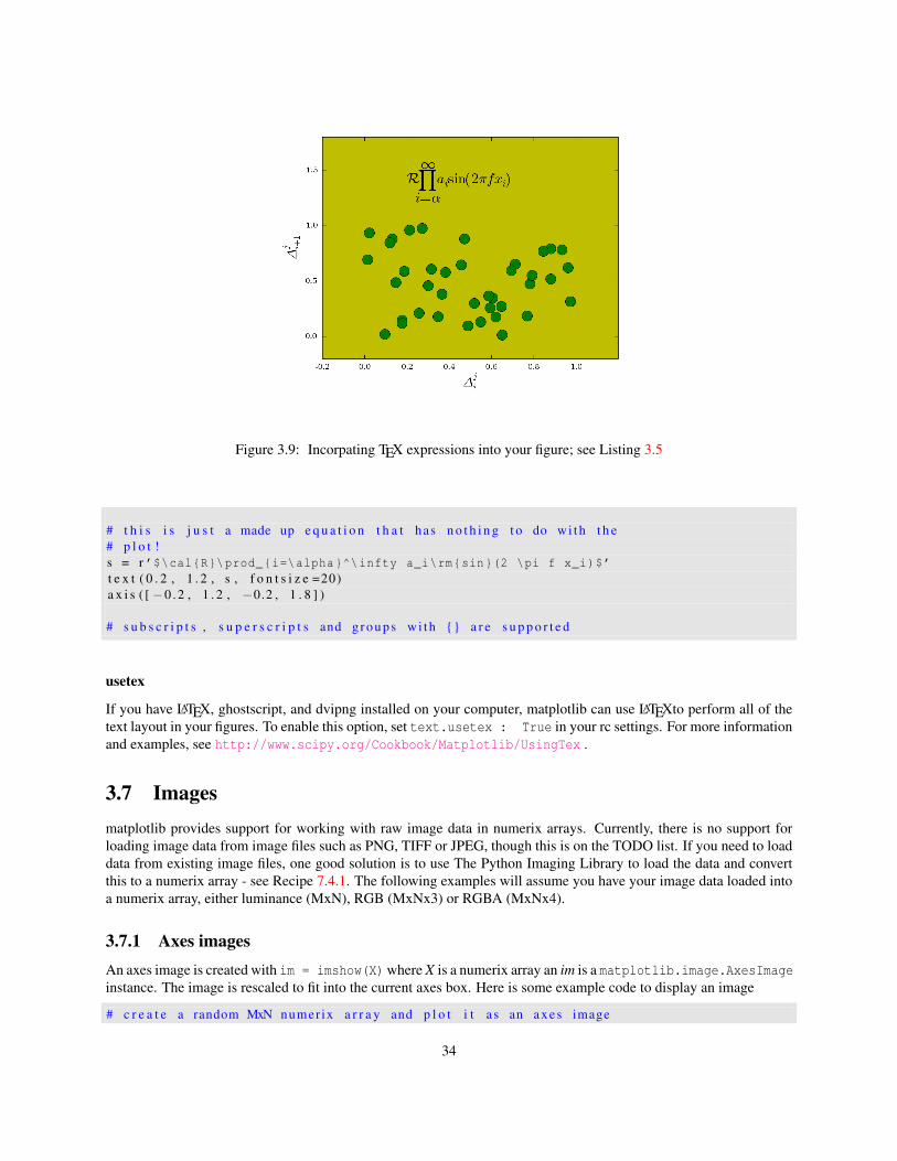
Figure 3.9: Incorpating TEX expressions into your figure; see Listing 3.5

# t h i s i s j u s t a made up e q u a t i o n t h a t has n o t h i n g t o do wi th t h e# p l o t !s = r ’$\cal{R}\prod_{i=\alpha}^\infty a_i\rm{sin}(2 \pi f x_i)$’t e x t ( 0 . 2 , 1 . 2 , s , f o n t s i z e =20)a x i s ( [ −0 .2 , 1 . 2 , −0.2 , 1 . 8 ] )

# s u b s c r i p t s , s u p e r s c r i p t s and g r ou ps wi th {} a r e s u p p o r t e d

usetex

If you have LATEX, ghostscript, and dvipng installed on your computer, matplotlib can use LATEXto perform all of thetext layout in your figures. To enable this option, set text.usetex : True in your rc settings. For more informationand examples, see http://www.scipy.org/Cookbook/Matplotlib/UsingTex .

3.7 Imagesmatplotlib provides support for working with raw image data in numerix arrays. Currently, there is no support forloading image data from image files such as PNG, TIFF or JPEG, though this is on the TODO list. If you need to loaddata from existing image files, one good solution is to use The Python Imaging Library to load the data and convertthis to a numerix array - see Recipe 7.4.1. The following examples will assume you have your image data loaded intoa numerix array, either luminance (MxN), RGB (MxNx3) or RGBA (MxNx4).

3.7.1 Axes imagesAn axes image is created with im = imshow(X)where X is a numerix array an im is a matplotlib.image.AxesImageinstance. The image is rescaled to fit into the current axes box. Here is some example code to display an image

# c r e a t e a random MxN numerix a r r a y and p l o t i t a s an axes image

34

from p y l a b import ∗X = rand ( 2 0 , 2 0 )im = imshow (X)

imshow a command in the pylab interface. This is a thin wrapper of the matplotlib.Axes.imshow method, whichcan be called from any Axes instance, eg ax.imshow(X).

There are two parameters that determine how the image is resampled into the axes bounding box: interpolationand aspect. The following interpolation schemes are available: bicubic, bilinear, blackman100, blackman256, black-man64, nearest, sinc144, sinc256, sinc64, spline16, and spline36. The default interpolation method is given by thevalue of image.interpolation in your matplotlibrc file. aspect can be either equal, auto, or some number, whichwill constrain the aspect ratio of the image. The default aspect setting is given by the value of the rc parameterimage.aspect.

The full syntax of the imshow command is

imshow (X, # t h e numer ix a r r a ycmap = None , # t h e m a t p l o t l i b . c o l o r s . Colormap i n s t a n c enorm = None , # t h e n o r m a l i z a t i o n i n s t a n c ea s p e c t =None , # t h e a s p e c t s e t t i n gi n t e r p o l a t i o n =None , # t h e i n t e r p o l a t i o n methoda l p h a = 1 . 0 , # t h e a l p h a t r a n s p a r e n c y v a l u evmin = None , # t h e min f o r image s c a l i n gvmax = None , # t h e max f o r image s c a l i n go r i g i n =None ) : # t h e image o r i g i n

When None, these parameters will assume a default value, in many cases determined by the rc setting. The meaningof cmap, norm, vmin, vmax, and origin will be explained in sections below.

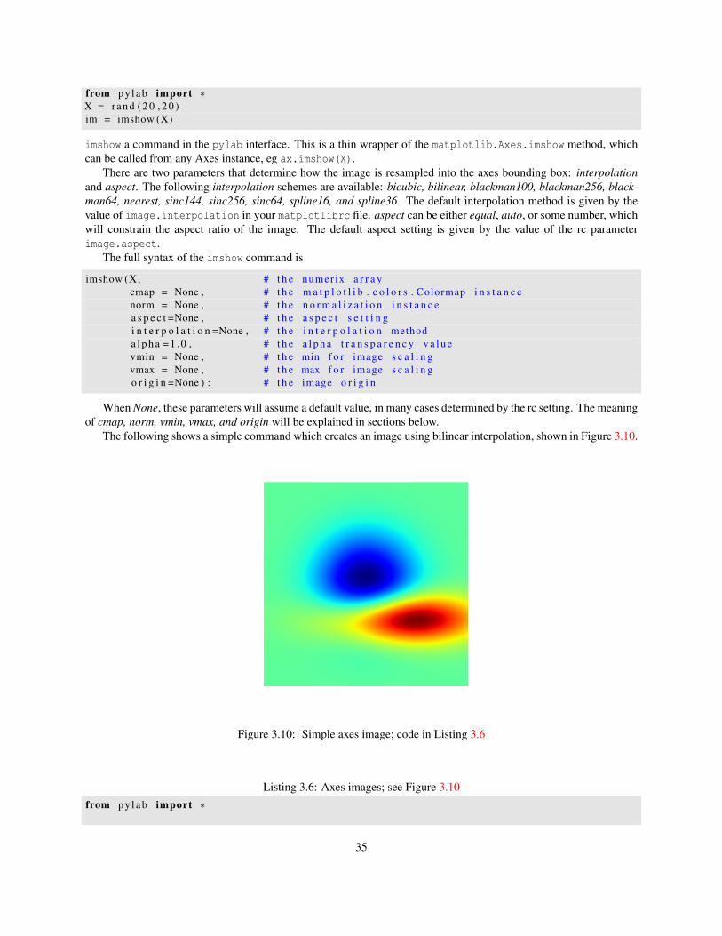
The following shows a simple command which creates an image using bilinear interpolation, shown in Figure 3.10.

Figure 3.10: Simple axes image; code in Listing 3.6

Listing 3.6: Axes images; see Figure 3.10from p y l a b import ∗

35

d e l t a = 0 .025# g e n e r a t e a mesh of x and y v e c t o r sx = y = a r a n g e ( −3.0 , 3 . 0 , d e l t a )X, Y = meshgr id ( x , y )# c r e a t e 2D g a u s s i a n d i s t r i b u t i o n sZ1 = b i v a r i a t e _ n o r m a l (X, Y, 1 . 0 , 1 . 0 , 0 . 0 , 0 . 0 )Z2 = b i v a r i a t e _ n o r m a l (X, Y, 1 . 5 , 0 . 5 , 1 , 1 )

# p l o t t h e d i f f e r e n c e o f G a u s s i a n s wi th b l i n e a r i n t e r p o l a t i o nim = imshow ( Z2−Z1 , i n t e r p o l a t i o n =’bilinear’ )a x i s ( ’off’ )

You can create an arbitrary number of axes images inside a single axes, and these will be composed via alphablending. However, if you want to blend several images, you must make sure that the hold state is True and that thealpha of the layered images is less than 1.0; if alpha=1.0 then the image on top will totally obscure the images below.Because the image blending is done using antigrain (regardless of your backend choice), you can blend images evenon backends which don’t support alpha (eg, postscript). This is because the alpha blending is done in the frontend andthe blended image is transferred directly to the backend as an RGB pixel array. See Recipe 7.4.2 for an example ofhow to layer images.

3.7.2 Figure imagesOften times you want to be able to look at your raw image data directly, without interpolation. This is the function offigure images, which do a pixel-by-pixel transfer of your image data to the figure canvas 1. Figure images are drawnfirst, and thus can become the background of other matplotlib drawing commands.

In the pylab interface, figure images are created with the figimage command, which unlike imshow, does notaccept an interpolation or aspect keyword argument because no image resampling is used. If the pixel extent of thefigure image extends beyond the figure canvas, the image will simply be truncated. The basic syntax is figimage(X,xo=0, yo=0) where X is luminance (MxN), RGB (MxNx3) or RGBA (MxNx4) numerix array and xo, yo are pixeloffsets from the origin (see Section 3.7.4). You can use figimage to create a figure image that fills the entire canvaswith no x or y offsets, or you can make multiple calls to figimage with different x and y offsets to create a mosaic ofimages, as shown in Recipe 7.4.3.

The full syntax of the figimage command is

f i g i m a g e (X, # t h e numer ix a r r a yxo =0 , # t h e x o f f s e tyo =0 , # t h e y o f f s e ta l p h a = 1 . 0 , # t h e a l p h a t r a n s p a r e n c ynorm=None , # t h e m a t p l o t l i b . c o l o r s . n o r m a l i z a t i o n i n s t a n c ecmap=None , # t h e m a t p l o t l i b . c o l o r s . Colormap i n s t a n c evmin=None , # t h e min f o r image s c a l i n gvmax=None , # t h e max f o r image s c a l i n go r i g i n =None ) # t h e image o r i g i n

The cmap, norm, vmin, vmax and origin arguments are explained in the sections below.pylab.figimage is a thin wrapper of matplotlib.figure.figimage and you can generate figure images di-

rectly with the pythonic API using fig.figimage(X) where fig is a Figure instance.

3.7.3 Scaling and color mappingIn addition to supporting raw image RGB and RGBA formats, matplotlib will scale and map luminance data forMxN float (luminance) arrays. The conversion from luminance data to RGBA occurs in two steps: scaling and colormapping.

1If you want a resampled image to occupy the full space of the figure canvas, you can achieve this by specifying a custom axes that fills thefigure canvas axes([0, 1, 0, 1]) and using imshow.

36

Scaling is the process of normalizing an MxN floating point array to the 0,1 interval, by mapping vmin to 0.0and vmax to 1.0, where vmin and vmax are user defined parameters. If either are None, the min and max of theimage data will be used, respectively. Scaling is handled by a matplotlib.colors.normalization instance, whichdefaults to normalization(vmin=None, vmax=None) - ie, the default is to scale the image so that the minimum ofthe luminance array is zero and the maximum of the luminance array is one.

Typically, you will not create a normalization instance yourself, but may set vmin or vmax in the keyword argu-ments of the image creation function. In this case, a normalization instance is created for you, and your vmin, vmaxsettings are applied. If you do supply a normalization instance for the norm argument, vmin and vmax will be ignored.See Table 3.5 for some examples of image normalization commands and their interpretation.

command interpretation»> imshow(X) X ≤ min(X)→ 0 and X ≥ max(X)→ 1»> imshow(X, vmax=10) X ≤ min(X)→ 0 and X ≥ 10 → 1»> imshow(X, vmin=0, vmax=10) X ≤ 0 → 0 and X ≥ 10 → 1»> anorm=normalize(2,8)»> imshow(X, norm=anorm) X ≤ 2 → 0 and X ≥ 8 → 1

Table 3.5: Example image normalization commands and their interpretation

Once the luminance data are normalized, they color mapper transforms the normalized data to RGBA using amatplotlib.colors.Colormap instance. Common colormaps are defined in matplotlib.cm, including cm.jet andcm.gray. If the cmap argument to an image command is None, the default is given by he rc parameter image.cmap.

The keyword arguments cmap, norm, vmin, vmax control color mapping and scaling in the image constructioncommands. Once the images have been created, several commands exist to interactively control the color map of thecurrent image. Like the current figure (gcf) and the current axes (gca), matplotlib keeps track of the current image(gci) to determine which image to apply the commands which affect image properties. To interactively set the imagenormalization limits, use clim(vmin=None, vmax=None), where vmin and vmax have the same meaning as above. Tointeractively change the colormap, use jet or gray (More colormaps and colormap commands are planned).. Theselatter commands not only change the colormap of the current image, they also set the default for future images.

For quantitative plotting of pseduocolor images, use the colorbar function to provide a colorbar associated withthe image, Here is an example interactive session controlling image scaling and color mapping with a colorbar

>>> imshow (X) # p l o t t h e luminance image X>>> c l im (−1 ,2) # s c a l e t h e image>>> j e t ( ) # use co lormap j e t>>> c o l o r b a r ( ) # add a c o l o r b a r t o t h e c u r r e n t axes>>> gray ( ) # use g r a y s c a l e ; image and c o l o r b a r a r e u p d a t e d

The image scaling and color mapping are handled by the mixin base class matplotlib.colors.ScalarMappable.

3.7.4 Image originDepending on your data, it may be more natural to plot your data with the image origin up (X[0,0] is upper left) ordown (X[0,0] is lower left). matplotlib supports these two modes with the origin parameter, which can be supplied asan optional keyword argument to the image commands imshow and figimage with the default set by the rc parameterimage.origin. To plot an image with the origin in the upper left, pass origin=’upper’ and with the image in thelower left, pass origin=’lower’, as shown in Figure 3.11.

Listing 3.7: Setting the image origin; see Figure 3.11from p y l a b import ∗

x = a r a n g e ( 1 0 0 . 0 ) ; x . shape = 10 ,10

s u b p l o t ( 2 1 1 )

37

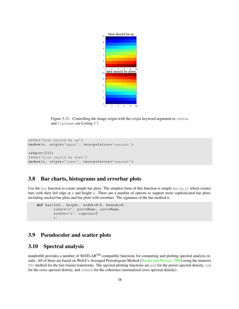
Figure 3.11: Controlling the image origin with the origin keyword argument to imshowand figimage; see Listing 3.7.

t i t l e ( ’blue should be up’ )imshow ( x , o r i g i n =’upper’ , i n t e r p o l a t i o n =’nearest’ )

s u b p l o t ( 2 1 2 )t i t l e ( ’blue should be down’ )imshow ( x , o r i g i n =’lower’ , i n t e r p o l a t i o n =’nearest’ )

3.8 Bar charts, histograms and errorbar plotsUse the bar function to create simple bar plots. The simplest form of this function is simply bar(x,y) which createsbars with their left edge at x and height y. There are a number of options to support more sophisticated bar plots,including stacked bar plots and bar plots with errorbars. The signature of the bar method is

def b a r ( l e f t , h e i g h t , w id th = 0 . 8 , bot tom =0 ,c o l o r =’b’ , y e r r =None , x e r r =None ,e c o l o r =’k’ , c a p s i z e =3) :

3.9 Pseudocolor and scatter plots

3.10 Spectral analysismatplotlib provides a number of MATLABTM compatible functions for computing and plotting spectral analysis re-sults. All of them are based on Welch’s Averaged Periodogram Method [Bendat and Piersol, 1986] using the numerixfft method for the fast fourier transforms. The spectral plotting functions are psd for the power spectral density, csdfor the cross spectral density, and cohere for the coherence (normalized cross spectral density).

38

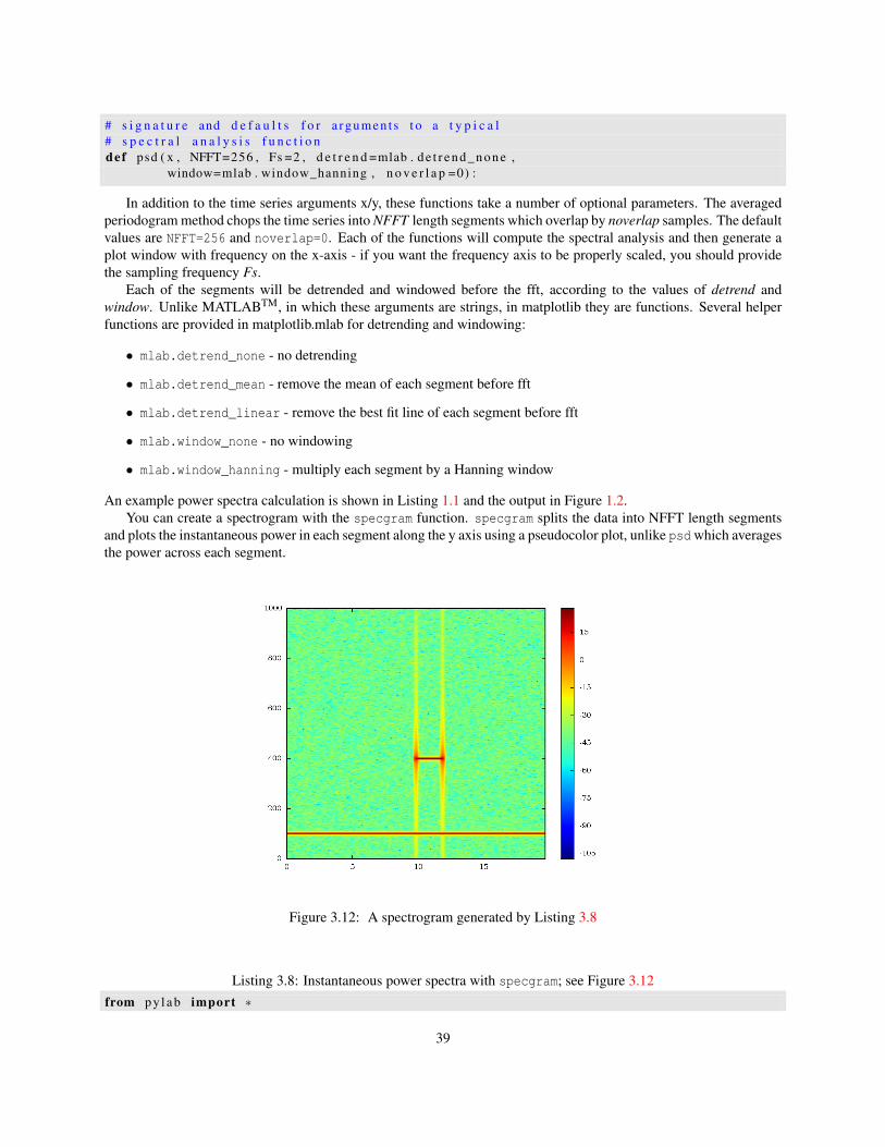
# s i g n a t u r e and d e f a u l t s f o r a rgumen t s t o a t y p i c a l# s p e c t r a l a n a l y s i s f u n c t i o ndef psd ( x , NFFT=256 , Fs =2 , d e t r e n d =mlab . d e t r e nd _n on e ,

window=mlab . window_hanning , n o v e r l a p =0) :

In addition to the time series arguments x/y, these functions take a number of optional parameters. The averagedperiodogram method chops the time series into NFFT length segments which overlap by noverlap samples. The defaultvalues are NFFT=256 and noverlap=0. Each of the functions will compute the spectral analysis and then generate aplot window with frequency on the x-axis - if you want the frequency axis to be properly scaled, you should providethe sampling frequency Fs.

Each of the segments will be detrended and windowed before the fft, according to the values of detrend andwindow. Unlike MATLABTM, in which these arguments are strings, in matplotlib they are functions. Several helperfunctions are provided in matplotlib.mlab for detrending and windowing:

• mlab.detrend_none - no detrending

• mlab.detrend_mean - remove the mean of each segment before fft

• mlab.detrend_linear - remove the best fit line of each segment before fft

• mlab.window_none - no windowing

• mlab.window_hanning - multiply each segment by a Hanning window

An example power spectra calculation is shown in Listing 1.1 and the output in Figure 1.2.You can create a spectrogram with the specgram function. specgram splits the data into NFFT length segments

and plots the instantaneous power in each segment along the y axis using a pseudocolor plot, unlike psd which averagesthe power across each segment.

Figure 3.12: A spectrogram generated by Listing 3.8

Listing 3.8: Instantaneous power spectra with specgram; see Figure 3.12from p y l a b import ∗

39

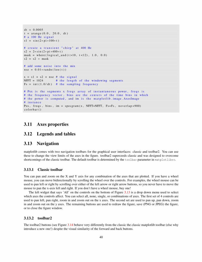
d t = 0 .0005t = a r a n g e ( 0 . 0 , 2 0 . 0 , d t )# a 100 Hz s i g n a ls1 = s i n (2∗ p i ∗100∗ t )

# c r e a t e a t r a n s i e n t " c h i r p " a t 400 Hzs2 = 2∗ s i n (2∗ p i ∗400∗ t )mask = where ( l o g i c a l _ a n d ( t >10 , t <12) , 1 . 0 , 0 . 0 )s2 = s2 ∗ mask

# add some n o i s e i n t o t h e mixnse = 0 .01∗ r andn ( l e n ( t ) )

x = s1 + s2 + nse # t h e s i g n a lNFFT = 1024 # t h e l e n g t h o f t h e windowing segmen t sFs = i n t ( 1 . 0 / d t ) # t h e s a m p l i n g f r e q u e n c y

# Pxx i s t h e segmen t s x f r e q s a r r a y o f i n s t a n t a n e o u s power , f r e q s i s# t h e f r e q u e n c y v e c t o r , b i n s a r e t h e c e n t e r s o f t h e t ime b i n s i n which# t h e power i s computed , and im i s t h e m a t p l o t l i b . image . AxesImage# i n s t a n c ePxx , f r e q s , b in s , im = specgram ( x , NFFT=NFFT , Fs=Fs , n o v e r l a p =900)c o l o r b a r ( )

3.11 Axes properties

3.12 Legends and tables

3.13 Navigationmatplotlib comes with two navigation toolbars for the graphical user interfaces: classic and toolbar2. You can usethese to change the view limits of the axes in the figure. toolbar2 superceeds classic and was designed to overcomeshortcomings of the classic toolbar. The default toolbar is determined by the toolbar parameter in matplotlibrc.

3.13.1 Classic toolbar

You can pan and zoom on the X and Y axis for any combination of the axes that are plotted. If you have a wheelmouse, you can move bidirectionally by scrolling the wheel over the controls. For examples, the wheel mouse can beused to pan left or right by scrolling over either of the left arrow or right arrow buttons, so you never have to move themouse to pan the x-axis left and right. If you don’t have a wheel mouse, buy one!

The left widget that says ’All’ on the controls on the bottom of Figure 3.13 is a drop down menu used to selectwhich axes the controls affect. You can select all, none, single, or combinations of axes. The first set of 4 controls areused to pan left, pan right, zoom in and zoom out on the x axes. The second set are used to pan up, pan down, zoomin and zoom out on the y axes. The remaining buttons are used to redraw the figure, save (PNG or JPEG) the figure,or to close the figure window.

3.13.2 toolbar2

The toolbar2 buttons (see Figure 3.14 behave very differently from the classic the classic matplotlib toolbar (else whyintroduce a new one!) despite the visual similarity of the forward and back buttons.

40

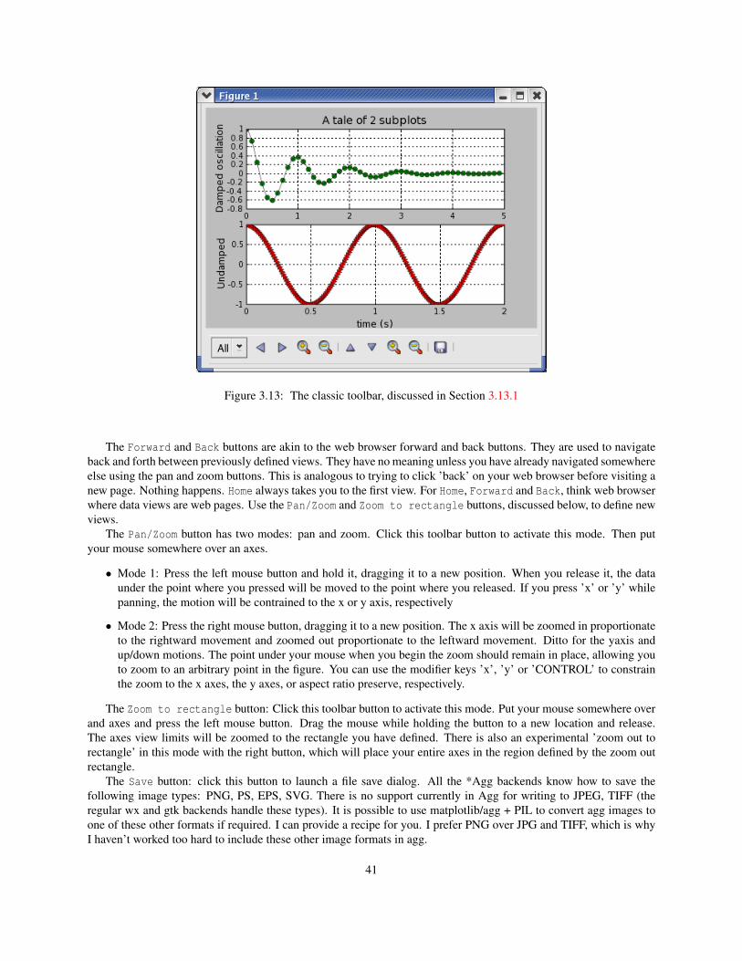
Figure 3.13: The classic toolbar, discussed in Section 3.13.1

The Forward and Back buttons are akin to the web browser forward and back buttons. They are used to navigateback and forth between previously defined views. They have no meaning unless you have already navigated somewhereelse using the pan and zoom buttons. This is analogous to trying to click ’back’ on your web browser before visiting anew page. Nothing happens. Home always takes you to the first view. For Home, Forward and Back, think web browserwhere data views are web pages. Use the Pan/Zoom and Zoom to rectangle buttons, discussed below, to define newviews.

The Pan/Zoom button has two modes: pan and zoom. Click this toolbar button to activate this mode. Then putyour mouse somewhere over an axes.

• Mode 1: Press the left mouse button and hold it, dragging it to a new position. When you release it, the dataunder the point where you pressed will be moved to the point where you released. If you press ’x’ or ’y’ whilepanning, the motion will be contrained to the x or y axis, respectively

• Mode 2: Press the right mouse button, dragging it to a new position. The x axis will be zoomed in proportionateto the rightward movement and zoomed out proportionate to the leftward movement. Ditto for the yaxis andup/down motions. The point under your mouse when you begin the zoom should remain in place, allowing youto zoom to an arbitrary point in the figure. You can use the modifier keys ’x’, ’y’ or ’CONTROL’ to constrainthe zoom to the x axes, the y axes, or aspect ratio preserve, respectively.

The Zoom to rectangle button: Click this toolbar button to activate this mode. Put your mouse somewhere overand axes and press the left mouse button. Drag the mouse while holding the button to a new location and release.The axes view limits will be zoomed to the rectangle you have defined. There is also an experimental ’zoom out torectangle’ in this mode with the right button, which will place your entire axes in the region defined by the zoom outrectangle.

The Save button: click this button to launch a file save dialog. All the *Agg backends know how to save thefollowing image types: PNG, PS, EPS, SVG. There is no support currently in Agg for writing to JPEG, TIFF (theregular wx and gtk backends handle these types). It is possible to use matplotlib/agg + PIL to convert agg images toone of these other formats if required. I can provide a recipe for you. I prefer PNG over JPG and TIFF, which is whyI haven’t worked too hard to include these other image formats in agg.

41

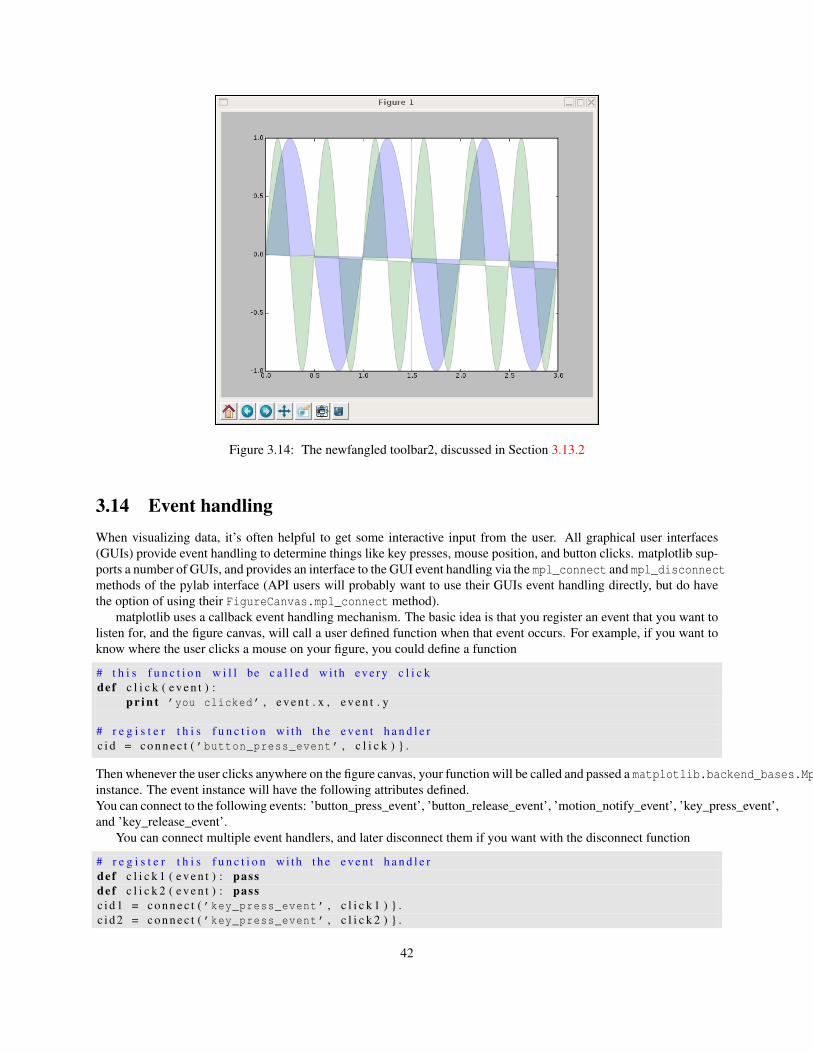
Figure 3.14: The newfangled toolbar2, discussed in Section 3.13.2

3.14 Event handlingWhen visualizing data, it’s often helpful to get some interactive input from the user. All graphical user interfaces(GUIs) provide event handling to determine things like key presses, mouse position, and button clicks. matplotlib sup-ports a number of GUIs, and provides an interface to the GUI event handling via the mpl_connect and mpl_disconnectmethods of the pylab interface (API users will probably want to use their GUIs event handling directly, but do havethe option of using their FigureCanvas.mpl_connect method).

matplotlib uses a callback event handling mechanism. The basic idea is that you register an event that you want tolisten for, and the figure canvas, will call a user defined function when that event occurs. For example, if you want toknow where the user clicks a mouse on your figure, you could define a function

# t h i s f u n c t i o n w i l l be c a l l e d wi th e v e r y c l i c kdef c l i c k ( e v e n t ) :

p r i n t ’you clicked’ , e v e n t . x , e v e n t . y

# r e g i s t e r t h i s f u n c t i o n wi th t h e e v e n t h a n d l e rc i d = c o n n e c t ( ’button_press_event’ , c l i c k ) } .

Then whenever the user clicks anywhere on the figure canvas, your function will be called and passed a matplotlib.backend_bases.MplEventinstance. The event instance will have the following attributes defined.You can connect to the following events: ’button_press_event’, ’button_release_event’, ’motion_notify_event’, ’key_press_event’,and ’key_release_event’.

You can connect multiple event handlers, and later disconnect them if you want with the disconnect function

# r e g i s t e r t h i s f u n c t i o n wi th t h e e v e n t h a n d l e rdef c l i c k 1 ( e v e n t ) : passdef c l i c k 2 ( e v e n t ) : passc i d 1 = c o n n e c t ( ’key_press_event’ , c l i c k 1 ) } .c i d 2 = c o n n e c t ( ’key_press_event’ , c l i c k 2 ) } .

42

Property Meaningx x position - pixels from left of canvasy y position - pixels from bottom of canvasbutton button pressed None, 1, 2, 3inaxes the Axes instance if mouse is over axes (or None)xdata x coord of mouse in data coords (None if mouse isn’t over axes)ydata y coord of mouse in data coords (None if mouse isn’t over axes)name The string name of the eventcanvas The FigureCanvas instance the event occured inkey The key press if any, eg ’a’, ’b’, ’1’. Also records ’control and ’shift’

Table 3.6: The event attributes

. . . l a t e r on . . . .d i s c o n n e c t ( c i d 1 ) # now on ly c l i c k 2 i s c o n n e c t e d

Here’s an example to get the mouse location in data coordinates as the mouse moves

# Connect t o t h e mouse move e v e n t and p r i n t t h e l o c a t i o n o f t h e mouse# i n d a t a c o o r d i n a t e s i f t h e mouse i s ove r an axesfrom p y l a b import ∗

p l o t ( a r a n g e ( 1 0 ) )

def on_move ( e v e n t ) :# g e t t h e x and y p i x e l c o o r d sx , y = e v e n t . x , e v e n t . y

i f e v e n t . i n a x e s :p r i n t ’data coords’ , e v e n t . xda ta , e v e n t . y d a t a

c o n n e c t ( ’motion_notify_event’ , on_move )

show ( )

3.15 Customizing plot defaults

43

44

Chapter 4

Font finding and properties

matplotlib.fonts.font_manager is module for finding, managing, and using fonts across-platforms. This moduleprovides a single FontManager that can be shared across backends and platforms. The findfont() method returnsthe best TrueType (TTF) font file in the local or system font path that matches the specified FontProperties. TheFontManager also handles Adobe Font Metrics (AFM) font files for use by the PostScript backend.

The design is based on the W3C Cascading Style Sheet, Level 1 (CSS1) font specification (http://www.w3.org/TR/1998/REC-CSS2-19980512). Future versions may implement the Level 2 or 2.1 specifications.

The font.family property has five values: ’serif’ (e.g. Times), ’sans-serif’ (e.g. Helvetica), ’cursive’ (e.g. Zapf-Chancery), ’fantasy’ (e.g. Western), and ’monospace’ (e.g. Courier). Each of these font families has a default list offont names in decreasing order of priority associated with them. You describe which family you want by choosing,eg, family=’serif’, and the font manager will search the font.serif list looking for one of the named fonts on yoursystem. The lists are user configurable, and reside in your matplotlibrc.

This allows you to choose your family in your matplotlib script and the font manager will try and find the best fontno matter which platform you run on.

• The font.style property has three values: normal (or roman), italic or oblique. The oblique style will be usedfor italic, if it is not present.

• The font.variant property has two values: normal or small-caps. For TrueType fonts, which are scalablefonts, small-caps is equivalent to using a font size of ’smaller’, or about 83

• The font.weight property has effectively 13 values: normal, bold, bolder, lighter, 100, 200, 300, ..., 900.Normal is the same as 400, and bold is 700. bolder and lighter are relative values with respect to the currentweight.

• The font.stretch property has 11 values: ultra-condensed, extra-condensed, condensed, semi-condensed,normal, semi-expanded, expanded, extra-expanded, ultra-expanded, wider, and narrower. This property is notcurrently implemented.

• The font.size property is the default font size for text, given in pts. 12pt is the standard value. Special textsizes for tick labels, axes, labels, title, etc. can be defined relative to font.size using the following values:xx-small, x-small, small, medium, large, x-large, xx-large, larger, or smaller. Special text sizes can also be anabsolute size, given in pts.

Here is an example using the font properties to illustrate the different fonts

from m a t p l o t l i b import r cPa ramsrcParams [ ’ps.useafm’ ]= F a l s efrom p y l a b import ∗

s u b p l o t ( 1 1 1 , a x i s b g =’w’ )

45

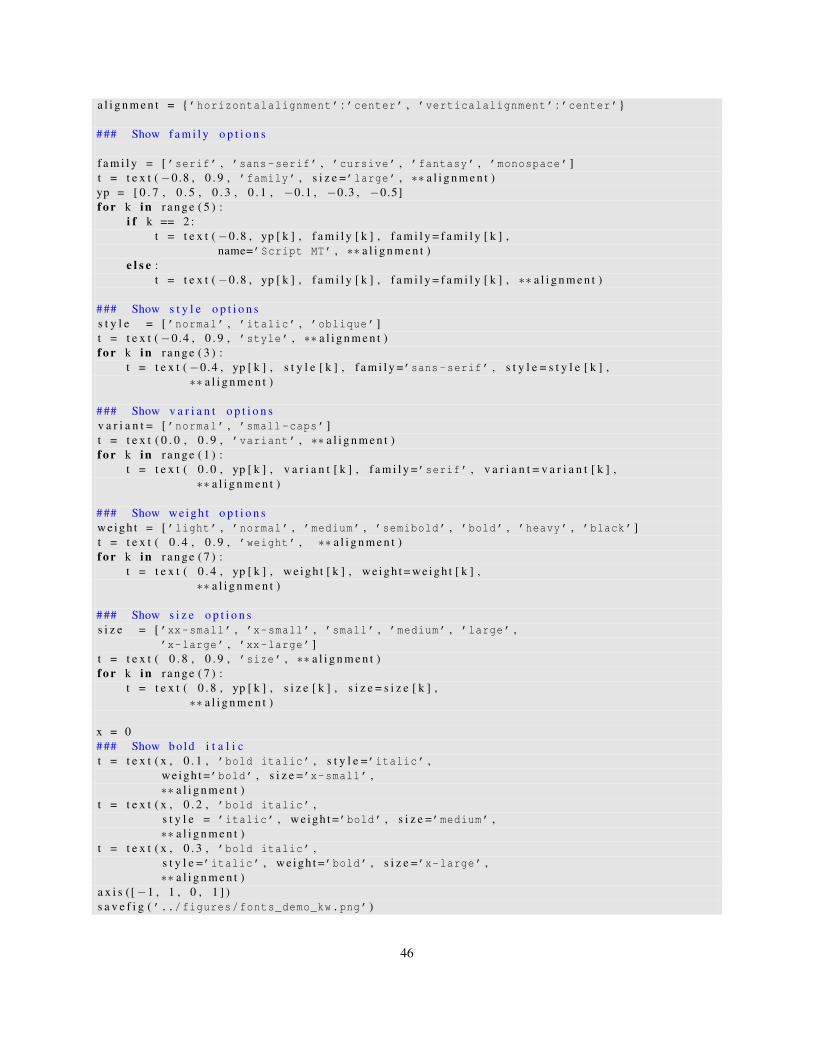
a l i g n m e n t = {’horizontalalignment’ : ’center’ , ’verticalalignment’ : ’center’}

### Show f a m i l y o p t i o n s

f a m i l y = [ ’serif’ , ’sans -serif’ , ’cursive’ , ’fantasy’ , ’monospace’ ]t = t e x t ( −0.8 , 0 . 9 , ’family’ , s i z e =’large’ , ∗∗ a l i g n m e n t )yp = [ 0 . 7 , 0 . 5 , 0 . 3 , 0 . 1 , −0.1 , −0.3 , −0.5]f o r k in r a n g e ( 5 ) :

i f k == 2 :t = t e x t ( −0.8 , yp [ k ] , f a m i l y [ k ] , f a m i l y = f a m i l y [ k ] ,

name=’Script MT’ , ∗∗ a l i g n m e n t )e l s e :

t = t e x t ( −0.8 , yp [ k ] , f a m i l y [ k ] , f a m i l y = f a m i l y [ k ] , ∗∗ a l i g n m e n t )

### Show s t y l e o p t i o n ss t y l e = [ ’normal’ , ’italic’ , ’oblique’ ]t = t e x t ( −0.4 , 0 . 9 , ’style’ , ∗∗ a l i g n m e n t )f o r k in r a n g e ( 3 ) :

t = t e x t ( −0.4 , yp [ k ] , s t y l e [ k ] , f a m i l y =’sans -serif’ , s t y l e = s t y l e [ k ] ,∗∗ a l i g n m e n t )

### Show v a r i a n t o p t i o n sv a r i a n t = [ ’normal’ , ’small -caps’ ]t = t e x t ( 0 . 0 , 0 . 9 , ’variant’ , ∗∗ a l i g n m e n t )f o r k in r a n g e ( 1 ) :

t = t e x t ( 0 . 0 , yp [ k ] , v a r i a n t [ k ] , f a m i l y =’serif’ , v a r i a n t = v a r i a n t [ k ] ,∗∗ a l i g n m e n t )

### Show we ig h t o p t i o n swe ig h t = [ ’light’ , ’normal’ , ’medium’ , ’semibold’ , ’bold’ , ’heavy’ , ’black’ ]t = t e x t ( 0 . 4 , 0 . 9 , ’weight’ , ∗∗ a l i g n m e n t )f o r k in r a n g e ( 7 ) :

t = t e x t ( 0 . 4 , yp [ k ] , we ig h t [ k ] , w e ig h t = w e ig h t [ k ] ,∗∗ a l i g n m e n t )

### Show s i z e o p t i o n ss i z e = [ ’xx-small’ , ’x-small’ , ’small’ , ’medium’ , ’large’ ,

’x-large’ , ’xx-large’ ]t = t e x t ( 0 . 8 , 0 . 9 , ’size’ , ∗∗ a l i g n m e n t )f o r k in r a n g e ( 7 ) :

t = t e x t ( 0 . 8 , yp [ k ] , s i z e [ k ] , s i z e = s i z e [ k ] ,∗∗ a l i g n m e n t )

x = 0### Show bo ld i t a l i ct = t e x t ( x , 0 . 1 , ’bold italic’ , s t y l e =’italic’ ,

we ig h t =’bold’ , s i z e =’x-small’ ,∗∗ a l i g n m e n t )

t = t e x t ( x , 0 . 2 , ’bold italic’ ,s t y l e = ’italic’ , w e ig h t =’bold’ , s i z e =’medium’ ,∗∗ a l i g n m e n t )

t = t e x t ( x , 0 . 3 , ’bold italic’ ,s t y l e =’italic’ , w e ig h t =’bold’ , s i z e =’x-large’ ,∗∗ a l i g n m e n t )

a x i s ([−1 , 1 , 0 , 1 ] )s a v e f i g ( ’../figures/fonts_demo_kw.png’ )

46

s a v e f i g ( ’../figures/fonts_demo_kw.eps’ )show ( )

47

48

Chapter 5

Collections

49

50

Chapter 6

Tick locators and formatters

The matplotlib.ticker module contains classes to support completely configurable tick locating and formatting.Although the locators know nothing about major or minor ticks, they are used by the Axis class to support majorand minor tick locating and formatting. Generic tick locators and formatters are provided, as well as domain specificcustom locators an formatters.

6.1 Tick locatingChoosing tick locations and formats is a difficult and essential part of making nice looking graphs. The matplotlib.tickermodule divides the workload between two bases classes: the locators and the formatters. Each axis (eg the xaxis andyaxis) has a major and minor tick locator and a major and minor tick formatter. The default minor tick locators alwaysreturn the empty list, ie, there are no minor ticks. Each of these can be set independently, and it is easy for the user tocreate and plug-in a custom tick locator or formatter.

The matplotlib.ticker.Locator class is the base class for all tick locators. The locators handle autoscalingof the view limits based on the data limits, and choosing the tick locations. The most generally useful tick locatoris MultipleLocator. You initialize this with a base, eg 10, and it picks axis limits and ticks that are multiples ofyour base. The class AutoLocator contains a MultipleLocator instance, and dynamically updates it based uponthe data and zoom limits. This should provide much more intelligent automatic tick locations both in figure creationand in navigation than in prior versions of matplotlib. See Tables 6.1 and 6.2 for a summary of the basic and date ticklocators.

Class SummaryNullLocator No ticksIndexLocator locator for index plots (eg where x = range(len(y))LinearLocator evenly spaced ticks from min to maxLogLocator logarithmically ticks from min to maxMultipleLocator ticks and range are a multiple of base; either integer or floatAutoLocator choose a MultipleLocator and dynamically reassign

Table 6.1: The basic tick locators

You can define your own locator by deriving from Locator. You must override the __call__ method, which returnsa sequence of locations, and you will probably want to override the autoscale method to set the view limits from thedata limits. If you want to override the default locator, use one of the above or a custom locator and pass it to the x ory axis instance. The relevant methods are

ax . x a x i s . s e t _ m a j o r _ l o c a t o r ( x m a j o r L o c a t o r )ax . x a x i s . s e t _ m i n o r _ l o c a t o r ( x m i n o r L o c a t o r )

51

Class SummaryMinuteLocator locate minutesHourLocator locate hoursDayLocator locate specifed days of the monthWeekdayLocator Locate days of the week, eg MO, TUMonthLocator locate months, eg 7 for julyYearLocator locate years that are multiples of baseRRuleLocator locate using a matplotlib.dates.rrulewrapper. The rrulewrapper is a simple wrapper around a dateutils.rrule https://moin.conectiva.com.br/DateUtil which allow almost arbitrary date tick specifications. See examples/date_demo_rrule.py.

Table 6.2: The tick locators specialized for date plots; these reside in thematplotlib.dates module

ax . y a x i s . s e t _ m a j o r _ l o c a t o r ( y m a j o r L o c a t o r )ax . y a x i s . s e t _ m i n o r _ l o c a t o r ( y m i n o r L o c a t o r )

The default minor locator is the NullLocator, eg no minor ticks on by default.

6.2 Tick formattingTick formatting is the process of converting the numeric tick location into a suitable string, and is controlled by classesderived from matplotlib.ticker.Formatter. The formatter operates on a single tick value (and its tick position)and returns a string to the axis. The tick formatters are summarized in Table 6.3.

Class SummaryNullFormatter no labels on the ticksFixedFormatter set the strings manually for the labelsFuncFormatter user defined function sets the labelsFormatStrFormatter use a sprintf format stringIndexFormatter cycle through fixed strings by tick positionScalarFormatter default formatter for scalars; autopick the fmt stringLogFormatter formatter for log axesDateFormatter use an strftime string to format the date

Table 6.3: The tick formatting classes

You can derive your own formatter from the Formatter base class by simply overriding the __call__ method. Theformatter class has access to the axis view and data limits.

To control the major and minor tick label formats, use one of the following methods::

ax . x a x i s . s e t _ m a j o r _ f o r m a t t e r ( x m a j o r F o r m a t t e r )ax . x a x i s . s e t _ m i n o r _ f o r m a t t e r ( x m i n o r F o r m a t t e r )ax . y a x i s . s e t _ m a j o r _ f o r m a t t e r ( y m a j o r F o r m a t t e r )ax . y a x i s . s e t _ m i n o r _ f o r m a t t e r ( y m i n o r F o r m a t t e r )

6.3 Example 1: major and minor ticksIn this example, the xaxis has major ticks that are multiples of 20 and minor ticks that are multiples of 5. The ticks areformatted with an integer format string formatter ’%d’. The minor ticks are unlabelled (NullFormatter).

The MultipleLocator ticker class is used to place ticks on multiples of some base. The FormatStrFormatteruses a string format string (eg’%d’ or ’%1.2f’ or ’%1.1f cm’ ) to format the tick.

52

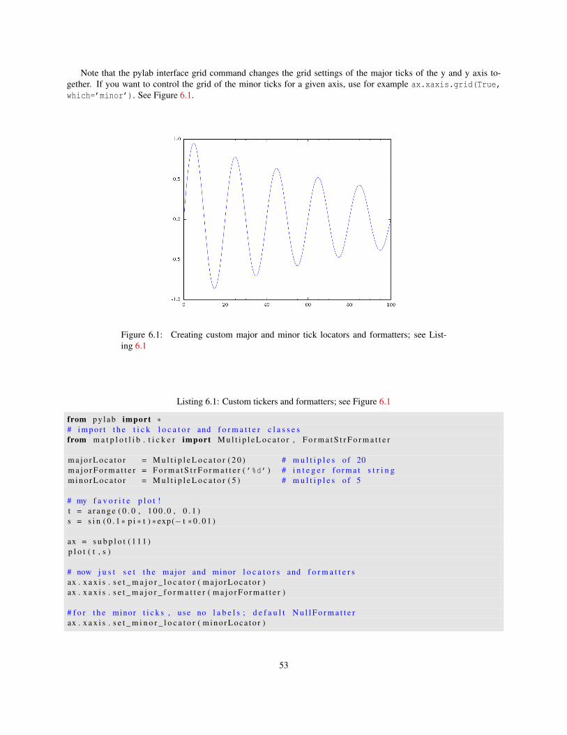
Note that the pylab interface grid command changes the grid settings of the major ticks of the y and y axis to-gether. If you want to control the grid of the minor ticks for a given axis, use for example ax.xaxis.grid(True,which=’minor’). See Figure 6.1.

Figure 6.1: Creating custom major and minor tick locators and formatters; see List-ing 6.1

Listing 6.1: Custom tickers and formatters; see Figure 6.1

from p y l a b import ∗# i m p o r t t h e t i c k l o c a t o r and f o r m a t t e r c l a s s e sfrom m a t p l o t l i b . t i c k e r import M u l t i p l e L o c a t o r , F o r m a t S t r F o r m a t t e r

m a j o r L o c a t o r = M u l t i p l e L o c a t o r ( 2 0 ) # m u l t i p l e s o f 20m a j o r F o r m a t t e r = F o r m a t S t r F o r m a t t e r ( ’%d’ ) # i n t e g e r f o r m a t s t r i n gm i n o r L o c a t o r = M u l t i p l e L o c a t o r ( 5 ) # m u l t i p l e s o f 5

# my f a v o r i t e p l o t !t = a r a n g e ( 0 . 0 , 1 0 0 . 0 , 0 . 1 )s = s i n ( 0 . 1 ∗ p i ∗ t ) ∗ exp(− t ∗0 . 0 1 )

ax = s u b p l o t ( 1 1 1 )p l o t ( t , s )

# now j u s t s e t t h e major and minor l o c a t o r s and f o r m a t t e r sax . x a x i s . s e t _ m a j o r _ l o c a t o r ( m a j o r L o c a t o r )ax . x a x i s . s e t _ m a j o r _ f o r m a t t e r ( m a j o r F o r m a t t e r )

# f o r t h e minor t i c k s , use no l a b e l s ; d e f a u l t N u l l F o r m a t t e rax . x a x i s . s e t _ m i n o r _ l o c a t o r ( m i n o r L o c a t o r )

53

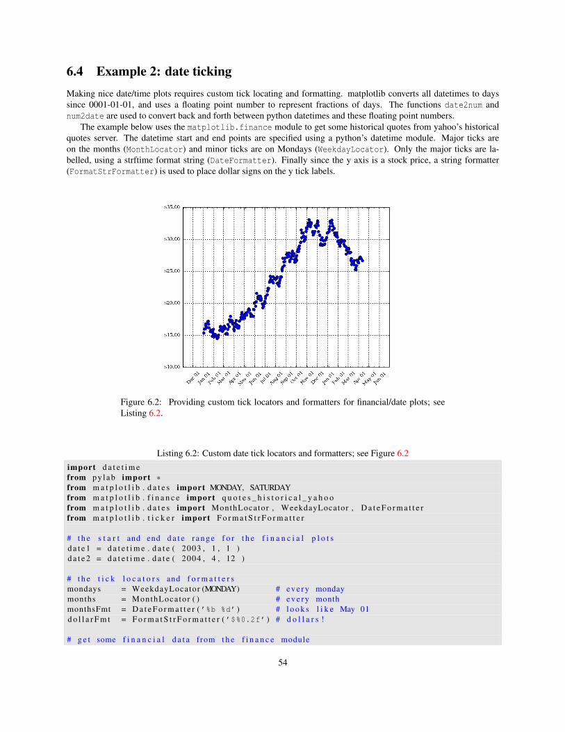
6.4 Example 2: date tickingMaking nice date/time plots requires custom tick locating and formatting. matplotlib converts all datetimes to dayssince 0001-01-01, and uses a floating point number to represent fractions of days. The functions date2num andnum2date are used to convert back and forth between python datetimes and these floating point numbers.

The example below uses the matplotlib.finance module to get some historical quotes from yahoo’s historicalquotes server. The datetime start and end points are specified using a python’s datetime module. Major ticks areon the months (MonthLocator) and minor ticks are on Mondays (WeekdayLocator). Only the major ticks are la-belled, using a strftime format string (DateFormatter). Finally since the y axis is a stock price, a string formatter(FormatStrFormatter) is used to place dollar signs on the y tick labels.

Figure 6.2: Providing custom tick locators and formatters for financial/date plots; seeListing 6.2.

Listing 6.2: Custom date tick locators and formatters; see Figure 6.2import d a t e t i m efrom p y l a b import ∗from m a t p l o t l i b . d a t e s import MONDAY, SATURDAYfrom m a t p l o t l i b . f i n a n c e import q u o t e s _ h i s t o r i c a l _ y a h o ofrom m a t p l o t l i b . d a t e s import MonthLocator , WeekdayLocator , D a t e F o r m a t t e rfrom m a t p l o t l i b . t i c k e r import F o r m a t S t r F o r m a t t e r

# t h e s t a r t and end d a t e r a n g e f o r t h e f i n a n c i a l p l o t sd a t e 1 = d a t e t i m e . d a t e ( 2003 , 1 , 1 )d a t e 2 = d a t e t i m e . d a t e ( 2004 , 4 , 12 )

# t h e t i c k l o c a t o r s and f o r m a t t e r smondays = WeekdayLocator (MONDAY) # e v e r y mondaymonths = MonthLocator ( ) # e v e r y monthmonthsFmt = D a t e F o r m a t t e r ( ’%b %d’ ) # l o o k s l i k e May 01d o l l a r F m t = F o r m a t S t r F o r m a t t e r ( ’$%0.2f’ ) # d o l l a r s !

# g e t some f i n a n c i a l d a t a from t h e f i n a n c e module

54

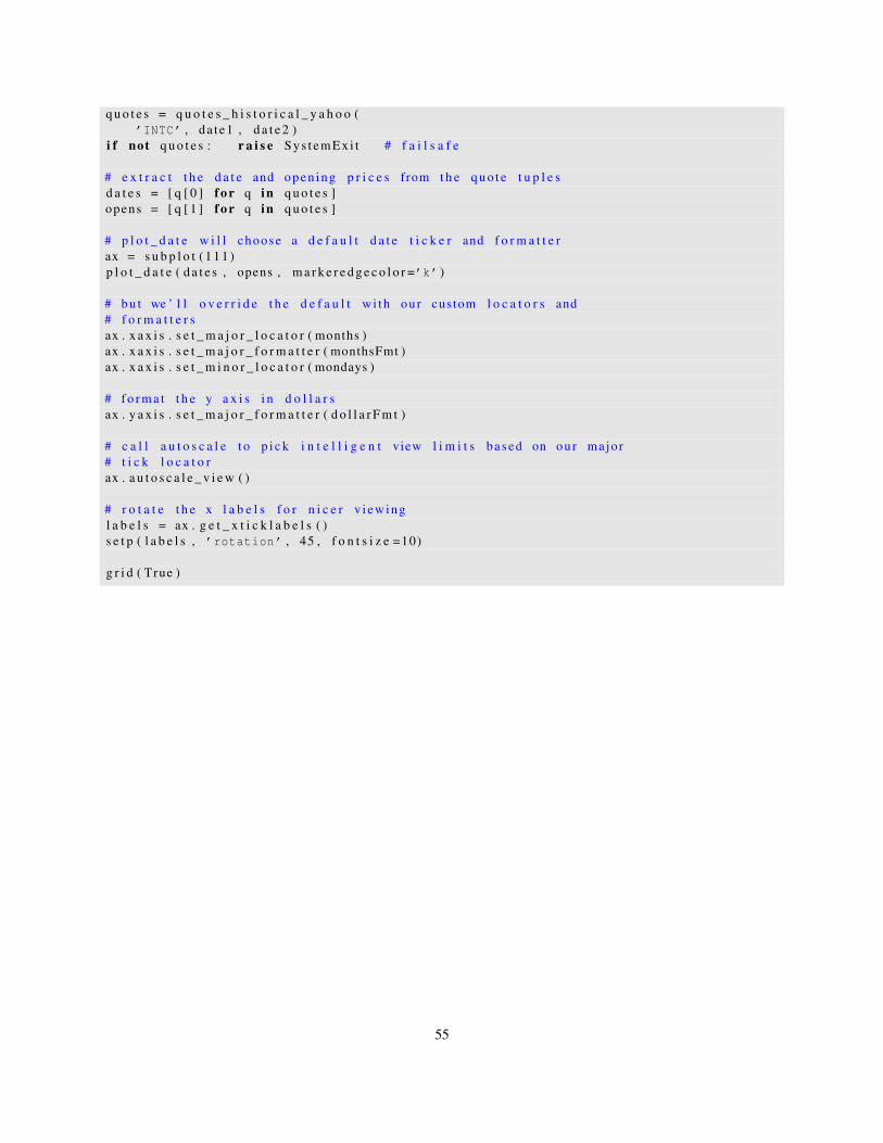
q u o t e s = q u o t e s _ h i s t o r i c a l _ y a h o o (’INTC’ , da t e1 , d a t e 2 )

i f not q u o t e s : r a i s e S y s t e m E x i t # f a i l s a f e

# e x t r a c t t h e d a t e and open ing p r i c e s from t h e q u o t e t u p l e sd a t e s = [ q [ 0 ] f o r q in q u o t e s ]opens = [ q [ 1 ] f o r q in q u o t e s ]

# p l o t _ d a t e w i l l choose a d e f a u l t d a t e t i c k e r and f o r m a t t e rax = s u b p l o t ( 1 1 1 )p l o t _ d a t e ( d a t e s , opens , m a r k e r e d g e c o l o r =’k’ )

# b u t we ’ l l o v e r r i d e t h e d e f a u l t w i th our custom l o c a t o r s and# f o r m a t t e r sax . x a x i s . s e t _ m a j o r _ l o c a t o r ( months )ax . x a x i s . s e t _ m a j o r _ f o r m a t t e r ( monthsFmt )ax . x a x i s . s e t _ m i n o r _ l o c a t o r ( mondays )

# f o r m a t t h e y a x i s i n d o l l a r sax . y a x i s . s e t _ m a j o r _ f o r m a t t e r ( d o l l a r F m t )

# c a l l a u t o s c a l e t o p i c k i n t e l l i g e n t view l i m i t s based on our major# t i c k l o c a t o rax . a u t o s c a l e _ v i e w ( )

# r o t a t e t h e x l a b e l s f o r n i c e r v i ewingl a b e l s = ax . g e t _ x t i c k l a b e l s ( )s e t p ( l a b e l s , ’rotation’ , 45 , f o n t s i z e =10)

g r i d ( True )

55

56

Chapter 7

Cookbook

7.1 Plot elements

7.1.1 Horizontal or vertical lines/spansIt is often useful to draw a line that stretches from the left to the right side of the axes at a given height, eg torepresent a y-axis threshold. In this case, the left and right are plotted in axes coordinates (0 and 1 respectively),and the y coordinate is in data coordinates. Plotted this way, the horizontal extent of the line will not change if youinteractively change the xlimits, eg by using the pan navigation tool. Although you can create these lines yourself usingmatplotlib.lines.Line2D instances and setting the appropriate transforms, several helper functions are providedto make this easier.

7.1.2 Fill the area between two curvesThe fill command takes a list of vertices and draws a polygon. A filled area between two curves is simply a largepolygon. All you need to do is get the vertices in the correct order, which basically means reversing the order of thex,y pairs in one of the lines, so that path across the vertices of the polygon is continuous. Here is a simple example

Listing 7.1: Fill the area between two curves; see Figure 7.1from p y l a b import ∗x1 = a r a n g e ( 0 , 2 , 0 . 0 1 )y1 = s i n (2∗ p i ∗x1 )y2 = s i n (4∗ p i ∗x1 ) + 2

# r e v e r s e x and y2 so t h e po lygon f i l l s i n o r d e rx = c o n c a t e n a t e ( ( x1 , x1 [ : : − 1 ] ) )y = c o n c a t e n a t e ( ( y1 , y2 [ : : − 1 ] ) )

p = f i l l ( x , y , f a c e c o l o r =’g’ )

7.2 Text

7.2.1 Adding a ylabel on the right of the axesTo make a ylabel on the right, use the text command. You need to set the transform to use axes coordinates(ax.transAxes), rotate the text vertically, make the horizontal alignment left, the vertical alignment centered. Notethat x, y = 1, 0.5 is the right, middle of the axes in axes coordinates. You also need to turn off clipping, so the text canappear outside the axes w/o being clipped by the axes bounding box, which is the default behavior.

57

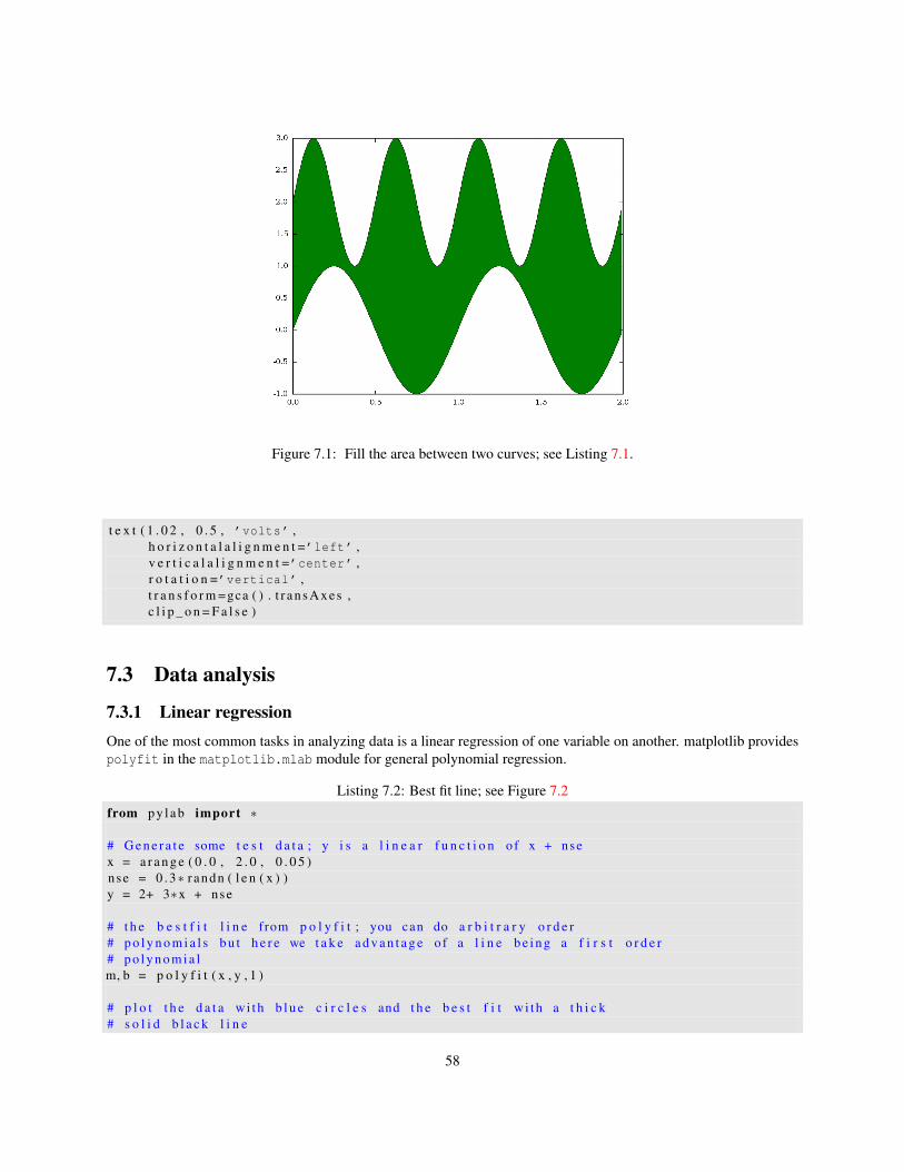
Figure 7.1: Fill the area between two curves; see Listing 7.1.

t e x t ( 1 . 0 2 , 0 . 5 , ’volts’ ,h o r i z o n t a l a l i g n m e n t =’left’ ,v e r t i c a l a l i g n m e n t =’center’ ,r o t a t i o n =’vertical’ ,t r a n s f o r m =gca ( ) . t r a n s A x e s ,c l i p _ o n = F a l s e )

7.3 Data analysis

7.3.1 Linear regressionOne of the most common tasks in analyzing data is a linear regression of one variable on another. matplotlib providespolyfit in the matplotlib.mlab module for general polynomial regression.

Listing 7.2: Best fit line; see Figure 7.2from p y l a b import ∗

# G e n e r a t e some t e s t d a t a ; y i s a l i n e a r f u n c t i o n o f x + nsex = a r a n g e ( 0 . 0 , 2 . 0 , 0 . 0 5 )nse = 0 . 3∗ r andn ( l e n ( x ) )y = 2+ 3∗x + nse

# t h e b e s t f i t l i n e from p o l y f i t ; you can do a r b i t r a r y o r d e r# p o l y n o m i a l s b u t h e r e we t a k e a d v a n t a g e o f a l i n e b e i n g a f i r s t o r d e r# p o l y n o m i a lm, b = p o l y f i t ( x , y , 1 )

# p l o t t h e d a t a wi th b l u e c i r c l e s and t h e b e s t f i t w i th a t h i c k# s o l i d b l a c k l i n e

58

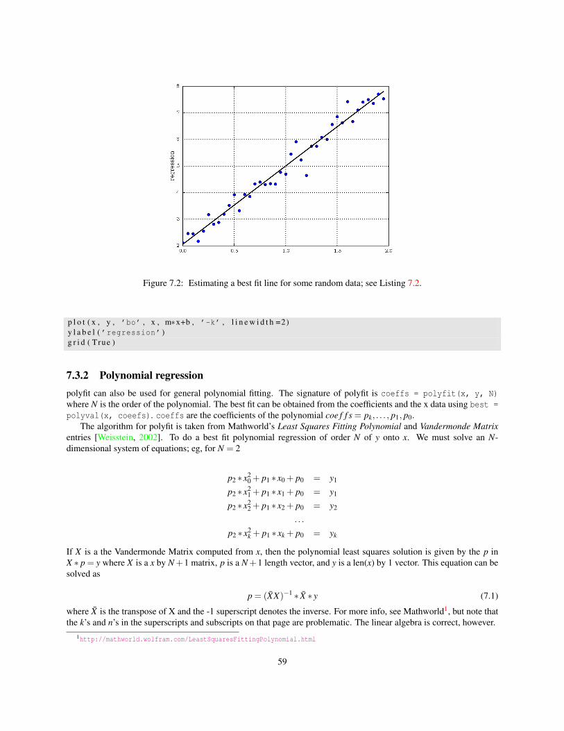
Figure 7.2: Estimating a best fit line for some random data; see Listing 7.2.

p l o t ( x , y , ’bo’ , x , m∗x+b , ’-k’ , l i n e w i d t h =2)y l a b e l ( ’regression’ )g r i d ( True )

7.3.2 Polynomial regressionpolyfit can also be used for general polynomial fitting. The signature of polyfit is coeffs = polyfit(x, y, N)where N is the order of the polynomial. The best fit can be obtained from the coefficients and the x data using best =polyval(x, coeefs). coeffs are the coefficients of the polynomial coe f f s = pk, . . . , p1, p0.

The algorithm for polyfit is taken from Mathworld’s Least Squares Fitting Polynomial and Vandermonde Matrixentries [Weisstein, 2002]. To do a best fit polynomial regression of order N of y onto x. We must solve an N-dimensional system of equations; eg, for N = 2

p2 ∗ x20 + p1 ∗ x0 + p0 = y1

p2 ∗ x21 + p1 ∗ x1 + p0 = y1

p2 ∗ x22 + p1 ∗ x2 + p0 = y2

. . .

p2 ∗ x2k + p1 ∗ xk + p0 = yk

If X is a the Vandermonde Matrix computed from x, then the polynomial least squares solution is given by the p inX ∗ p = y where X is a x by N +1 matrix, p is a N +1 length vector, and y is a len(x) by 1 vector. This equation can besolved as

p = (XX)−1 ∗ X ∗ y (7.1)

where X is the transpose of X and the -1 superscript denotes the inverse. For more info, see Mathworld1, but note thatthe k’s and n’s in the superscripts and subscripts on that page are problematic. The linear algebra is correct, however.

1http://mathworld.wolfram.com/LeastSquaresFittingPolynomial.html

59

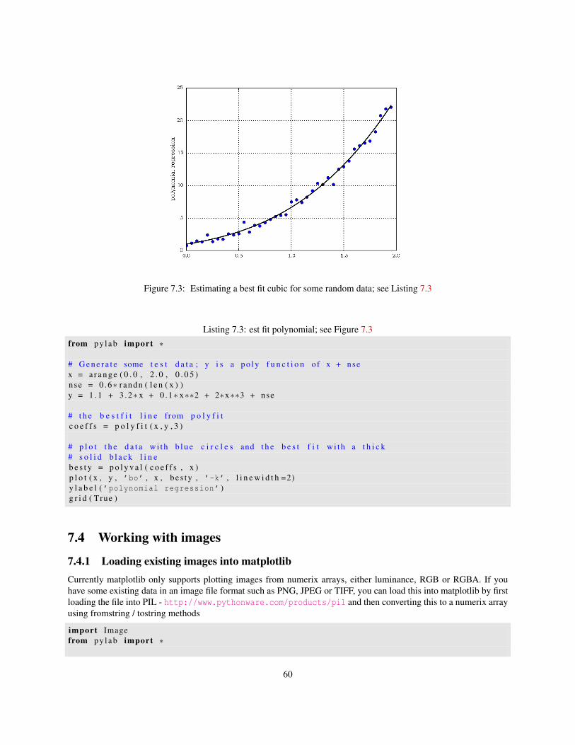
Figure 7.3: Estimating a best fit cubic for some random data; see Listing 7.3

Listing 7.3: est fit polynomial; see Figure 7.3from p y l a b import ∗

# G e n e r a t e some t e s t d a t a ; y i s a po ly f u n c t i o n o f x + nsex = a r a n g e ( 0 . 0 , 2 . 0 , 0 . 0 5 )nse = 0 . 6∗ r andn ( l e n ( x ) )y = 1 . 1 + 3 . 2∗ x + 0 . 1∗ x∗∗2 + 2∗x∗∗3 + nse

# t h e b e s t f i t l i n e from p o l y f i tc o e f f s = p o l y f i t ( x , y , 3 )

# p l o t t h e d a t a wi th b l u e c i r c l e s and t h e b e s t f i t w i th a t h i c k# s o l i d b l a c k l i n eb e s t y = p o l y v a l ( c o e f f s , x )p l o t ( x , y , ’bo’ , x , b e s t y , ’-k’ , l i n e w i d t h =2)y l a b e l ( ’polynomial regression’ )g r i d ( True )

7.4 Working with images

7.4.1 Loading existing images into matplotlibCurrently matplotlib only supports plotting images from numerix arrays, either luminance, RGB or RGBA. If youhave some existing data in an image file format such as PNG, JPEG or TIFF, you can load this into matplotlib by firstloading the file into PIL - http://www.pythonware.com/products/pil and then converting this to a numerix arrayusing fromstring / tostring methods

import Imagefrom p y l a b import ∗

60

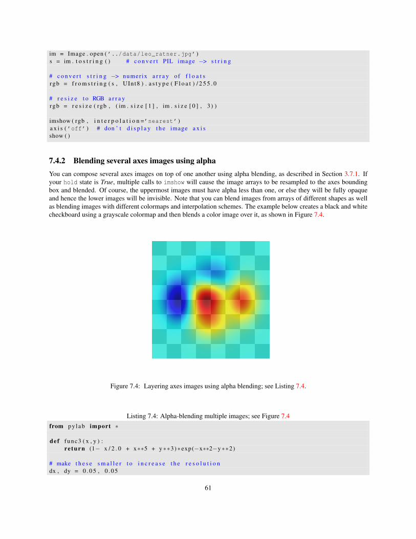
im = Image . open ( ’../data/leo_ratner.jpg’ )s = im . t o s t r i n g ( ) # c o n v e r t PIL image −> s t r i n g

# c o n v e r t s t r i n g −> numer ix a r r a y o f f l o a t srgb = f r o m s t r i n g ( s , UInt8 ) . a s t y p e ( F l o a t ) / 2 5 5 . 0

# r e s i z e t o RGB a r r a yrgb = r e s i z e ( rgb , ( im . s i z e [ 1 ] , im . s i z e [ 0 ] , 3 ) )

imshow ( rgb , i n t e r p o l a t i o n =’nearest’ )a x i s ( ’off’ ) # don ’ t d i s p l a y t h e image a x i sshow ( )

7.4.2 Blending several axes images using alphaYou can compose several axes images on top of one another using alpha blending, as described in Section 3.7.1. Ifyour hold state is True, multiple calls to imshow will cause the image arrays to be resampled to the axes boundingbox and blended. Of course, the uppermost images must have alpha less than one, or else they will be fully opaqueand hence the lower images will be invisible. Note that you can blend images from arrays of different shapes as wellas blending images with different colormaps and interpolation schemes. The example below creates a black and whitecheckboard using a grayscale colormap and then blends a color image over it, as shown in Figure 7.4.

Figure 7.4: Layering axes images using alpha blending; see Listing 7.4.

Listing 7.4: Alpha-blending multiple images; see Figure 7.4from p y l a b import ∗

def func3 ( x , y ) :re turn (1− x / 2 . 0 + x∗∗5 + y ∗∗3) ∗ exp(−x∗∗2−y ∗∗2)

# make t h e s e s m a l l e r t o i n c r e a s e t h e r e s o l u t i o ndx , dy = 0 . 0 5 , 0 . 0 5

61

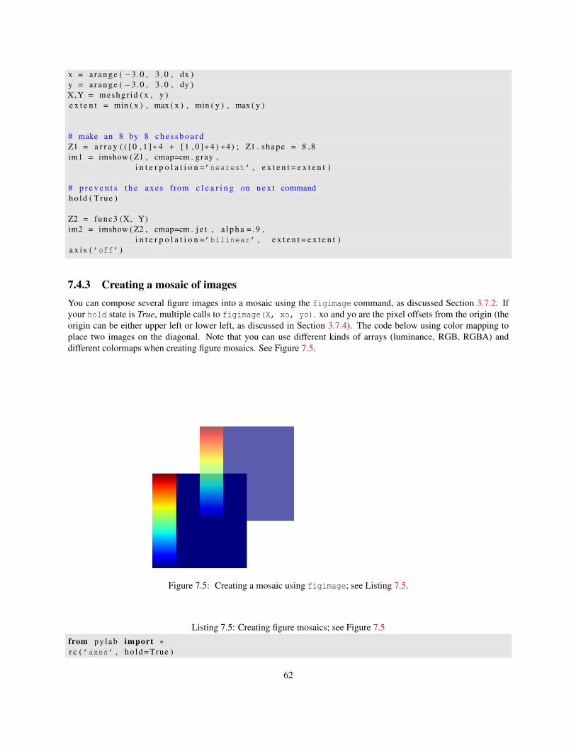
x = a r a n g e ( −3.0 , 3 . 0 , dx )y = a r a n g e ( −3.0 , 3 . 0 , dy )X,Y = meshgr id ( x , y )e x t e n t = min ( x ) , max ( x ) , min ( y ) , max ( y )

# make an 8 by 8 c h e s s b o a r dZ1 = a r r a y ( ( [ 0 , 1 ] ∗ 4 + [ 1 , 0 ] ∗ 4 ) ∗4) ; Z1 . shape = 8 ,8im1 = imshow ( Z1 , cmap=cm . gray ,

i n t e r p o l a t i o n =’nearest’ , e x t e n t = e x t e n t )

# p r e v e n t s t h e axes from c l e a r i n g on n e x t commandho ld ( True )

Z2 = func3 (X, Y)im2 = imshow ( Z2 , cmap=cm . j e t , a l p h a = . 9 ,

i n t e r p o l a t i o n =’bilinear’ , e x t e n t = e x t e n t )a x i s ( ’off’ )

7.4.3 Creating a mosaic of imagesYou can compose several figure images into a mosaic using the figimage command, as discussed Section 3.7.2. Ifyour hold state is True, multiple calls to figimage(X, xo, yo). xo and yo are the pixel offsets from the origin (theorigin can be either upper left or lower left, as discussed in Section 3.7.4). The code below using color mapping toplace two images on the diagonal. Note that you can use different kinds of arrays (luminance, RGB, RGBA) anddifferent colormaps when creating figure mosaics. See Figure 7.5.

Figure 7.5: Creating a mosaic using figimage; see Listing 7.5.

Listing 7.5: Creating figure mosaics; see Figure 7.5from p y l a b import ∗r c ( ’axes’ , ho ld =True )

62

r c ( ’image’ , o r i g i n =’upper’ )

Z = a r a n g e ( 4 0 0 0 0 . 0 ) ; Z . shape = 200 ,200Z [ : , 5 0 : ] = 1im1 = f i g i m a g e ( Z , xo =0 , yo =0)im2 = f i g i m a g e ( Z , xo =100 , yo =100 , a l p h a = . 8 )

7.4.4 Defining your own colormapPerry Greenfield has provided a nice framework with matplotlib.colors.LinearSegmentedColormap to definenew colormaps. You can create new colormaps fairly easy by following the example of jet in matplotlib.cm. Hereare the steps

• define your rgb linear segments in matplotlib.cm, following the lead of the _jet_data dictionary in that module

• add an entry to the datad dictionary in that module which maps rc string names for your color map to thedictionary you just defined.

• instantiate a single instance of your colormap in cm, following the example

j e t = c o l o r s . L inearSegmentedColormap ( ’jet’ , _ j e t _ d a t a , LUTSIZE )

• add a pylab function which has the same name as your colormap, following the example of pylab.jet.

Now anyone can use the colormap interactively from the shell, by setting it as the default image.cmap in rc, etc. Pleasesubmit your changes to the matplotlib-devel mailing list.

7.5 Output

7.5.1 Printing to standard outputIn some instances, it is nice to be able to print to a file object, eg sys.stdot, for example in a web application serverwhere the creation of a temporary file storing the images is a wasted step. The antigrain backend accepts a file objectto the savefig command and will print a PNG to it. Thus to print to standard output, you could do

import s y simport m a t p l o t l i b# t h i s i s n o t s u p p o r t e d a c r o s s a l l backends , a s o f m a t p l o t l i b −0.63m a t p l o t l i b . use ( ’Agg’ )from p y l a b import ∗p l o t ( [ 1 , 2 , 3 ] )s a v e f i g ( s y s . s t d o u t )

63

64

Chapter 8

Matplotlib API

The pylab interface does a lot of work for you under the hood, creating and managing multiple figure windows,directing your plotting commands to the current axes and figure, managing the interactive state, and so on. But that isall it does: all of the plotting is handled by a set of classes that the user can instantiate directly. If you are developinga GUI application, or simply don’t want any hidden magic in your plots, you can create any plots using pure OO codethat you could create with the pylab interface.

From a developer standpoint, the pylab interface has been a blessing in disguise. Because the interface was fixedby the Mathworks before the start of matplotlib provided considerable freedom to redesign the guts of the plottinglibrary – the object model can be totally revamped and the user interface remains fixed.

The matplotlib code is divided conceptually into 3 parts: the MATLABTM interface, the matplotlib Artists, and thebackend renderers. The pylab interface was covered in Chapter 3. This module pylab is comprised mainly of codeto manage the multiple figure windows across backends, and provide a thin, procedural wrapper around the objectoriented plotting code. The matplotlib Artists are a series of classes that derive from matplotlib.artist.Artist,so named because these are the objects that actually draw into the figure; see Figure 8.3. The backend renderers eachimplement a common drawing interface that actually puts the ink on the paper, eg creating a postscript document,filling an antigrain pixel buffer, or calling the gtk drawing code.

This chapter delves into matplotlib internals to give a clearer picture of how things work and how they are orga-nized. Some of this material may be of interest only to developers, but most of it should shed light for anyone whowants to be able to exploit the full capabilities of matplotlib. The normal path of figure creation in matplotlib is pylabinterface → creates artists → calls to the backend renderer. This section will invert that process, starting with thebackend, which is where the drawing actually takes place. This is the natural order of presentation because the back-end knows nothing about Artists, which in turn known nothing about the pylab interface. After the overview of thebackend API, there is a discussion of the matplotlib artists; this is the section that is most useful to users, particularlythose who want to embed matplotlib in an application. The final section shows how the pylab interface controls thebackends and artists – this section is probably of interest to developers and the terminally curious.

8.1 The matplotlib backends

The backend consists of a number of related base classes that together define a drawing API. The original backend wasGTK, and the drawing API is heavily based on the GTK drawing model, which is very simple. There are three essentialclasses defined in matplotlib.backend_bases: RendererBase, GraphicsContextBase and FigureCanvasBase. Inaddition, there are some classes for use with the GUI backends to define the interface to the toolbars and eventhandling. The RendererBase, aka renderer handles all the drawing primitives in display coordinates, typical renderermethods are draw_text and draw_lines. The GraphicsContextBase, aka textitgraphics context stores informationabout the graphics properties, such as linewidth, cap or join style, color, alpha translucency. The FigureCanvasBase,aka figure canvas, is primarily a container class to hold the Figure instance; this facilitates separation of the Figurefrom the backend dependent code. For GUI backends, the figure canvas should be a GUI widget embeddable in a GUI

65

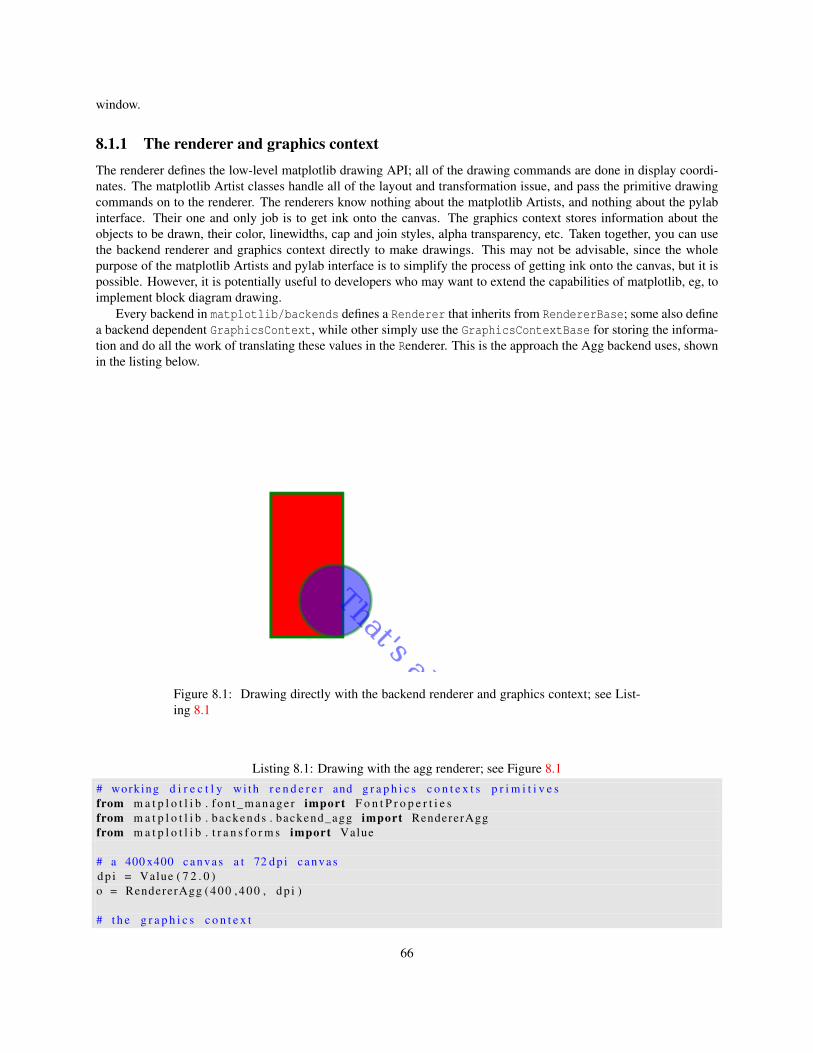
window.

8.1.1 The renderer and graphics contextThe renderer defines the low-level matplotlib drawing API; all of the drawing commands are done in display coordi-nates. The matplotlib Artist classes handle all of the layout and transformation issue, and pass the primitive drawingcommands on to the renderer. The renderers know nothing about the matplotlib Artists, and nothing about the pylabinterface. Their one and only job is to get ink onto the canvas. The graphics context stores information about theobjects to be drawn, their color, linewidths, cap and join styles, alpha transparency, etc. Taken together, you can usethe backend renderer and graphics context directly to make drawings. This may not be advisable, since the wholepurpose of the matplotlib Artists and pylab interface is to simplify the process of getting ink onto the canvas, but it ispossible. However, it is potentially useful to developers who may want to extend the capabilities of matplotlib, eg, toimplement block diagram drawing.

Every backend in matplotlib/backends defines a Renderer that inherits from RendererBase; some also definea backend dependent GraphicsContext, while other simply use the GraphicsContextBase for storing the informa-tion and do all the work of translating these values in the Renderer. This is the approach the Agg backend uses, shownin the listing below.

Figure 8.1: Drawing directly with the backend renderer and graphics context; see List-ing 8.1

Listing 8.1: Drawing with the agg renderer; see Figure 8.1# working d i r e c t l y wi th r e n d e r e r and g r a p h i c s c o n t e x t s p r i m i t i v e sfrom m a t p l o t l i b . f o n t _ m a n a g e r import F o n t P r o p e r t i e sfrom m a t p l o t l i b . backends . backend_agg import RendererAggfrom m a t p l o t l i b . t r a n s f o r m s import Value

# a 400 x400 c an va s a t 72 d p i c an va sd p i = Value ( 7 2 . 0 )o = RendererAgg ( 4 0 0 , 4 0 0 , d p i )

# t h e g r a p h i c s c o n t e x t

66

gc = o . new_gc ( )

# draw t h e background w h i t egc . s e t _ f o r e g r o u n d ( ’w’ )f a c e = ( 1 , 1 , 1 ) # w h i t eo . d r a w _ r e c t a n g l e ( gc , f ace , 0 , 0 , 400 , 400)

# t h e gc ’ s know a b o u t c o l o r s t r i n g s , and can h a n d l e any m a t p l o t l i b# c o l o r a rgumen t s ( hex s t r i n g s , rgb , f o r m a t s t r i n g s , e t c )gc . s e t _ f o r e g r o u n d ( ’g’ )gc . s e t _ l i n e w i d t h ( 4 )f a c e = ( 1 , 0 , 0 ) # must be rgbo . d r a w _ r e c t a n g l e ( gc , f ace , 10 , 50 , 100 , 200)

# draw a t r a n s l u c e n t e l l i p s ergb = ( 0 , 0 , 1 )gc . s e t _ a l p h a ( 0 . 5 )o . d raw_arc ( gc , rgb , 100 , 100 , 100 , 100 , 360 , 360 , 0 )

# draw a dashed l i n egc . s e t _ d a s h e s ( 0 , [ 5 , 1 0 ] )gc . s e t _ j o i n s t y l e ( ’miter’ )gc . s e t _ c a p s t y l e ( ’butt’ )gc . s e t _ l i n e w i d t h ( 3 . 0 )# broken wi th new API#o . d r a w _ l i n e s ( gc , ( 5 0 , 100 , 150 , 200 , 250) , ( 4 0 0 , 100 , 300 , 200 , 250) )

# draw some t e x t u s i n g t h e m a t p l o t l i b f o n t managerprop = F o n t P r o p e r t i e s ( s i z e =40)gc . s e t _ f o r e g r o u n d ( ’b’ )o . d r a w _ t e x t ( gc , 100 , 300 , "That’s all folks!" , prop , −45, 0 )

# t h e r e i s no s t a n d a r d r e n d e r e r i n t e r f a c e t o save t h e i n p u t t o a f i l e ,# as t h i s i s t h e j o b of t h e f i g u r e c an va s . Here I make t h e c a l l t h a t# t h e f i g u r e c an va s would make f o r t h e a n t i g r a i n r e n d e ro . _ r e n d e r e r . w r i t e _ p n g ( ’../figures/renderer_agg.png’ )

8.1.2 The figure canvases

8.2 The matplotlib Artists

8.3 pylab interface internals

Let’s look at the simplest matplotlib script and walk through what happens under the hood. This section will be ofinterest mainly to developers or those curious about matplotlib internals - it can be safely skipped by others. We’llassume you are using one of the GUI backends, eg GTKAgg and have are running this as a script (interactive :False)

from p y l a b import ∗p l o t ( [ 1 , 2 , 3 ] )show ( )

67

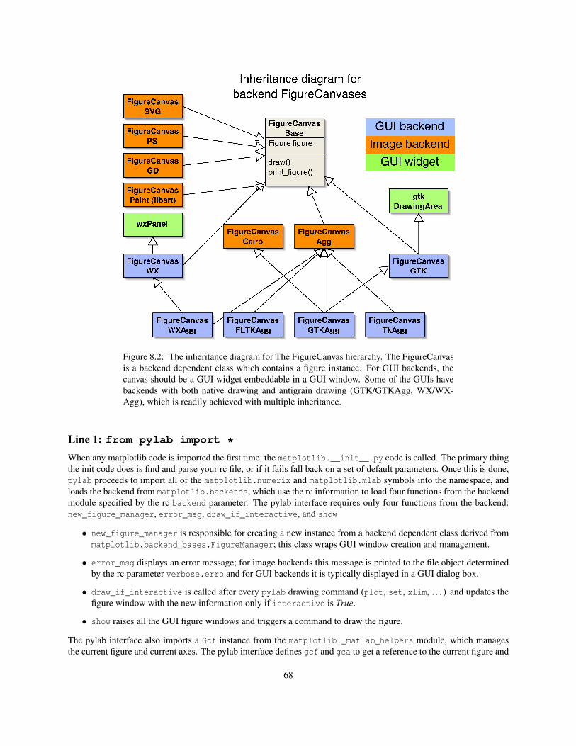
Figure 8.2: The inheritance diagram for The FigureCanvas hierarchy. The FigureCanvasis a backend dependent class which contains a figure instance. For GUI backends, thecanvas should be a GUI widget embeddable in a GUI window. Some of the GUIs havebackends with both native drawing and antigrain drawing (GTK/GTKAgg, WX/WX-Agg), which is readily achieved with multiple inheritance.

Line 1: from pylab import *

When any matplotlib code is imported the first time, the matplotlib.__init__.py code is called. The primary thingthe init code does is find and parse your rc file, or if it fails fall back on a set of default parameters. Once this is done,pylab proceeds to import all of the matplotlib.numerix and matplotlib.mlab symbols into the namespace, andloads the backend from matplotlib.backends, which use the rc information to load four functions from the backendmodule specified by the rc backend parameter. The pylab interface requires only four functions from the backend:new_figure_manager, error_msg, draw_if_interactive, and show

• new_figure_manager is responsible for creating a new instance from a backend dependent class derived frommatplotlib.backend_bases.FigureManager; this class wraps GUI window creation and management.

• error_msg displays an error message; for image backends this message is printed to the file object determinedby the rc parameter verbose.erro and for GUI backends it is typically displayed in a GUI dialog box.

• draw_if_interactive is called after every pylab drawing command (plot, set, xlim, . . . ) and updates thefigure window with the new information only if interactive is True.

• show raises all the GUI figure windows and triggers a command to draw the figure.

The pylab interface also imports a Gcf instance from the matplotlib._matlab_helpers module, which managesthe current figure and current axes. The pylab interface defines gcf and gca to get a reference to the current figure and

68

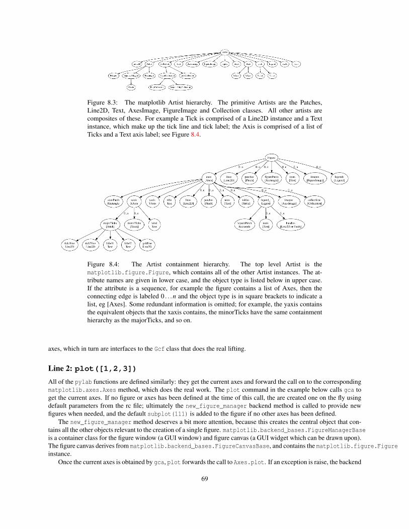
Figure 8.3: The matplotlib Artist hierarchy. The primitive Artists are the Patches,Line2D, Text, AxesImage, FigureImage and Collection classes. All other artists arecomposites of these. For example a Tick is comprised of a Line2D instance and a Textinstance, which make up the tick line and tick label; the Axis is comprised of a list ofTicks and a Text axis label; see Figure 8.4.

Figure 8.4: The Artist containment hierarchy. The top level Artist is thematplotlib.figure.Figure, which contains all of the other Artist instances. The at-tribute names are given in lower case, and the object type is listed below in upper case.If the attribute is a sequence, for example the figure contains a list of Axes, then theconnecting edge is labeled 0 . . .n and the object type is in square brackets to indicate alist, eg [Axes]. Some redundant information is omitted; for example, the yaxis containsthe equivalent objects that the xaxis contains, the minorTicks have the same containmenthierarchy as the majorTicks, and so on.

axes, which in turn are interfaces to the Gcf class that does the real lifting.

Line 2: plot([1,2,3])All of the pylab functions are defined similarly: they get the current axes and forward the call on to the correspondingmatplotlib.axes.Axes method, which does the real work. The plot command in the example below calls gca toget the current axes. If no figure or axes has been defined at the time of this call, the are created one on the fly usingdefault parameters from the rc file; ultimately the new_figure_manager backend method is called to provide newfigures when needed, and the default subplot(111) is added to the figure if no other axes has been defined.

The new_figure_manager method deserves a bit more attention, because this creates the central object that con-tains all the other objects relevant to the creation of a single figure. matplotlib.backend_bases.FigureManagerBaseis a container class for the figure window (a GUI window) and figure canvas (a GUI widget which can be drawn upon).The figure canvas derives from matplotlib.backend_bases.FigureCanvasBase, and contains the matplotlib.figure.Figureinstance.

Once the current axes is obtained by gca, plot forwards the call to Axes.plot. If an exception is raise, the backend

69

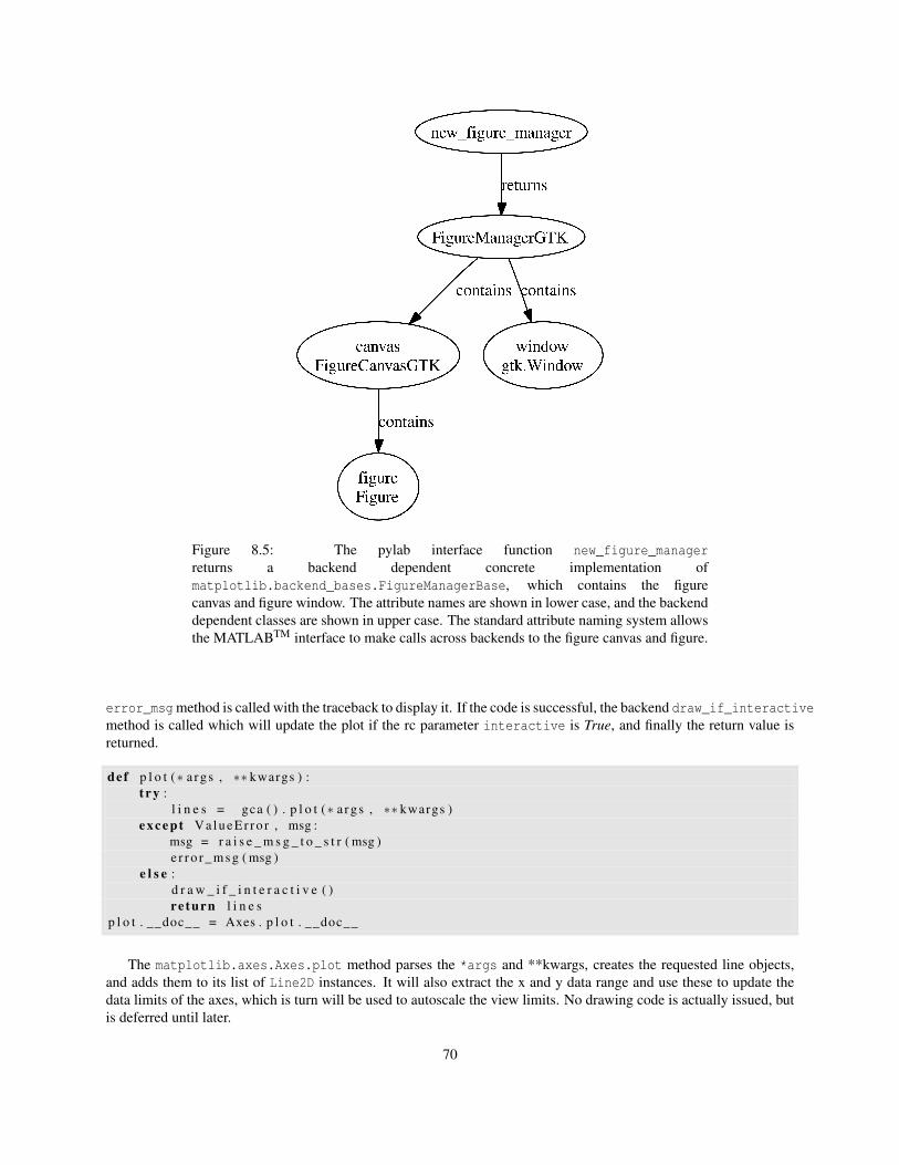
Figure 8.5: The pylab interface function new_figure_managerreturns a backend dependent concrete implementation ofmatplotlib.backend_bases.FigureManagerBase, which contains the figurecanvas and figure window. The attribute names are shown in lower case, and the backenddependent classes are shown in upper case. The standard attribute naming system allowsthe MATLABTM interface to make calls across backends to the figure canvas and figure.

error_msgmethod is called with the traceback to display it. If the code is successful, the backend draw_if_interactivemethod is called which will update the plot if the rc parameter interactive is True, and finally the return value isreturned.

def p l o t (∗ a rgs , ∗∗ kwargs ) :t r y :

l i n e s = gca ( ) . p l o t (∗ a rgs , ∗∗ kwargs )e xc ep t Val ueEr ro r , msg :

msg = r a i s e _ m s g _ t o _ s t r ( msg )e r r o r _ m s g ( msg )

e l s e :d r a w _ i f _ i n t e r a c t i v e ( )re turn l i n e s

p l o t . __doc__ = Axes . p l o t . __doc__

The matplotlib.axes.Axes.plot method parses the *args and **kwargs, creates the requested line objects,and adds them to its list of Line2D instances. It will also extract the x and y data range and use these to update thedata limits of the axes, which is turn will be used to autoscale the view limits. No drawing code is actually issued, butis deferred until later.

70

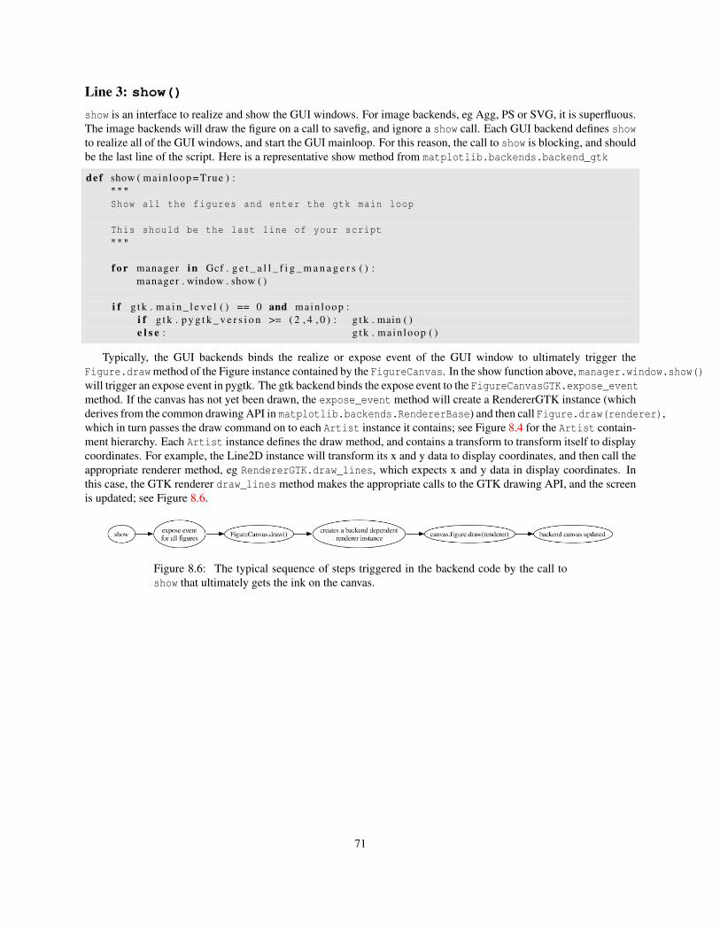
Line 3: show()show is an interface to realize and show the GUI windows. For image backends, eg Agg, PS or SVG, it is superfluous.The image backends will draw the figure on a call to savefig, and ignore a show call. Each GUI backend defines showto realize all of the GUI windows, and start the GUI mainloop. For this reason, the call to show is blocking, and shouldbe the last line of the script. Here is a representative show method from matplotlib.backends.backend_gtk

def show ( main loop =True ) :"""Show all the figures and enter the gtk main loop

This should be the last line of your script"""

f o r manager in Gcf . g e t _ a l l _ f i g _ m a n a g e r s ( ) :manager . window . show ( )

i f g t k . m a i n _ l e v e l ( ) == 0 and main loop :i f g t k . p y g t k _ v e r s i o n >= ( 2 , 4 , 0 ) : g t k . main ( )e l s e : g t k . main loop ( )

Typically, the GUI backends binds the realize or expose event of the GUI window to ultimately trigger theFigure.draw method of the Figure instance contained by the FigureCanvas. In the show function above, manager.window.show()will trigger an expose event in pygtk. The gtk backend binds the expose event to the FigureCanvasGTK.expose_eventmethod. If the canvas has not yet been drawn, the expose_event method will create a RendererGTK instance (whichderives from the common drawing API in matplotlib.backends.RendererBase) and then call Figure.draw(renderer),which in turn passes the draw command on to each Artist instance it contains; see Figure 8.4 for the Artist contain-ment hierarchy. Each Artist instance defines the draw method, and contains a transform to transform itself to displaycoordinates. For example, the Line2D instance will transform its x and y data to display coordinates, and then call theappropriate renderer method, eg RendererGTK.draw_lines, which expects x and y data in display coordinates. Inthis case, the GTK renderer draw_lines method makes the appropriate calls to the GTK drawing API, and the screenis updated; see Figure 8.6.

Figure 8.6: The typical sequence of steps triggered in the backend code by the call toshow that ultimately gets the ink on the canvas.

71

72

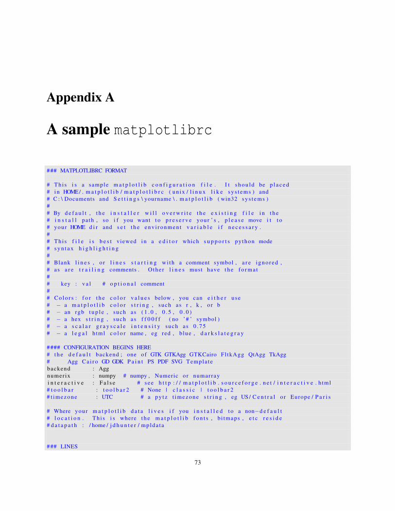
Appendix A

A sample matplotlibrc

### MATPLOTLIBRC FORMAT

# Th i s i s a sample m a t p l o t l i b c o n f i g u r a t i o n f i l e . I t s h o u l d be p l a c e d# i n HOME/ . m a t p l o t l i b / m a t p l o t l i b r c ( un ix / l i n u x l i k e s y s t e m s ) and# C : \ Documents and S e t t i n g s \ yourname \ . m a t p l o t l i b ( win32 s y s t e m s )## By d e f a u l t , t h e i n s t a l l e r w i l l o v e r w r i t e t h e e x i s t i n g f i l e i n t h e# i n s t a l l pa th , so i f you want t o p r e s e r v e your ’ s , p l e a s e move i t t o# your HOME d i r and s e t t h e e n v i r o n m e n t v a r i a b l e i f n e c e s s a r y .## Th i s f i l e i s b e s t viewed i n a e d i t o r which s u p p o r t s py thon mode# s y n t a x h i g h l i g h t i n g## Blank l i n e s , o r l i n e s s t a r t i n g wi th a comment symbol , a r e i g n o r e d ,# as a r e t r a i l i n g comments . O the r l i n e s must have t h e f o r m a t## key : v a l # o p t i o n a l comment## C o l o r s : f o r t h e c o l o r v a l u e s below , you can e i t h e r use# − a m a t p l o t l i b c o l o r s t r i n g , such as r , k , o r b# − an rgb t u p l e , such as ( 1 . 0 , 0 . 5 , 0 . 0 )# − a hex s t r i n g , such as f f 0 0 f f ( no ’# ’ symbol )# − a s c a l a r g r a y s c a l e i n t e n s i t y such as 0 . 7 5# − a l e g a l h tml c o l o r name , eg red , b lue , d a r k s l a t e g r a y

#### CONFIGURATION BEGINS HERE# t h e d e f a u l t backend ; one o f GTK GTKAgg GTKCairo Fl tkAgg QtAgg TkAgg# Agg C a i r o GD GDK P a i n t PS PDF SVG Templa tebackend : Aggnumer ix : numpy # numpy , Numeric o r numarrayi n t e r a c t i v e : F a l s e # s e e h t t p : / / m a t p l o t l i b . s o u r c e f o r g e . n e t / i n t e r a c t i v e . h tml# t o o l b a r : t o o l b a r 2 # None | c l a s s i c | t o o l b a r 2# t i m e z o n e : UTC # a p y t z t i m e z o n e s t r i n g , eg US / C e n t r a l o r Europe / P a r i s

# Where your m a t p l o t l i b d a t a l i v e s i f you i n s t a l l e d t o a non−d e f a u l t# l o c a t i o n . Th i s i s where t h e m a t p l o t l i b f o n t s , b i tmaps , e t c r e s i d e# d a t a p a t h : / home / j d h u n t e r / mp lda t a

### LINES

73

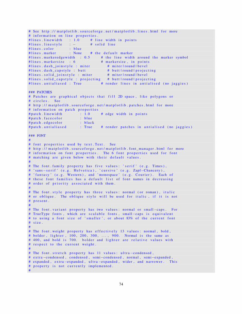
# See h t t p : / / m a t p l o t l i b . s o u r c e f o r g e . n e t / m a t p l o t l i b . l i n e s . h tml f o r more# i n f o r m a t i o n on l i n e p r o p e r t i e s .# l i n e s . l i n e w i d t h : 1 . 0 # l i n e wid th i n p o i n t s# l i n e s . l i n e s t y l e : − # s o l i d l i n e# l i n e s . c o l o r : b l u e# l i n e s . marker : None # t h e d e f a u l t marker# l i n e s . ma rk e redgewi d th : 0 . 5 # t h e l i n e wid th a round t h e marker symbol# l i n e s . m a r k e r s i z e : 6 # m a r k e r s i z e , i n p o i n t s# l i n e s . d a s h _ j o i n s t y l e : m i t e r # m i t e r | round | b e v e l# l i n e s . d a s h _ c a p s t y l e : b u t t # b u t t | round | p r o j e c t i n g# l i n e s . s o l i d _ j o i n s t y l e : m i t e r # m i t e r | round | b e v e l# l i n e s . s o l i d _ c a p s t y l e : p r o j e c t i n g # b u t t | round | p r o j e c t i n g# l i n e s . a n t i a l i a s e d : True # r e n d e r l i n e s i n a n t i a l i s e d ( no j a g g i e s )

### PATCHES# P a t c h e s a r e g r a p h i c a l o b j e c t s t h a t f i l l 2D space , l i k e p o l y go n s o r# c i r c l e s . See# h t t p : / / m a t p l o t l i b . s o u r c e f o r g e . n e t / m a t p l o t l i b . p a t c h e s . h tml f o r more# i n f o r m a t i o n on p a t c h p r o p e r t i e s# p a t c h . l i n e w i d t h : 1 . 0 # edge wid th i n p o i n t s# p a t c h . f a c e c o l o r : b l u e# p a t c h . e d g e c o l o r : b l a c k# p a t c h . a n t i a l i a s e d : True # r e n d e r p a t c h e s i n a n t i a l i s e d ( no j a g g i e s )

### FONT## f o n t p r o p e r t i e s used by t e x t . Text . See# h t t p : / / m a t p l o t l i b . s o u r c e f o r g e . n e t / m a t p l o t l i b . f o n t _ m a n a g e r . h tml f o r more# i n f o r m a t i o n on f o n t p r o p e r t i e s . The 6 f o n t p r o p e r t i e s used f o r f o n t# match ing a r e g i v e n below wi th t h e i r d e f a u l t v a l u e s .## The f o n t . f a m i l y p r o p e r t y has f i v e v a l u e s : ’ s e r i f ’ ( e . g . Times ) ,# ’ sans−s e r i f ’ ( e . g . H e l v e t i c a ) , ’ c u r s i v e ’ ( e . g . Zapf−Chancery ) ,# ’ f a n t a s y ’ ( e . g . Western ) , and ’ monospace ’ ( e . g . C o u r i e r ) . Each of# t h e s e f o n t f a m i l i e s has a d e f a u l t l i s t o f f o n t names i n d e c r e a s i n g# o r d e r o f p r i o r i t y a s s o c i a t e d wi th them .## The f o n t . s t y l e p r o p e r t y has t h r e e v a l u e s : normal ( o r roman ) , i t a l i c# o r o b l i q u e . The o b l i q u e s t y l e w i l l be used f o r i t a l i c , i f i t i s n o t# p r e s e n t .## The f o n t . v a r i a n t p r o p e r t y has two v a l u e s : normal o r sma l l−caps . For# TrueType f o n t s , which a r e s c a l a b l e f o n t s , sma l l−caps i s e q u i v a l e n t# t o u s i n g a f o n t s i z e o f ’ s m a l l e r ’ , o r a b o u t 83% of t h e c u r r e n t f o n t# s i z e .## The f o n t . we ig h t p r o p e r t y has e f f e c t i v e l y 13 v a l u e s : normal , bold ,# b o l d e r , l i g h t e r , 100 , 200 , 300 , . . . , 9 0 0 . Normal i s t h e same as# 400 , and bo ld i s 7 0 0 . b o l d e r and l i g h t e r a r e r e l a t i v e v a l u e s wi th# r e s p e c t t o t h e c u r r e n t we ig h t .## The f o n t . s t r e t c h p r o p e r t y has 11 v a l u e s : u l t r a −condensed ,# e x t r a−condensed , condensed , semi−condensed , normal , semi−expanded ,# expanded , e x t r a−expanded , u l t r a −expanded , wider , and n a r r o w e r . Th i s# p r o p e r t y i s n o t c u r r e n t l y implemented .#

74

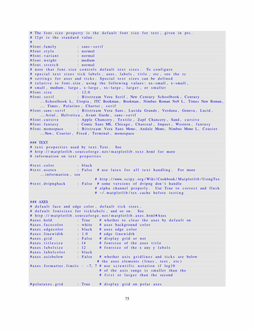
# The f o n t . s i z e p r o p e r t y i s t h e d e f a u l t f o n t s i z e f o r t e x t , g i v e n i n p t s .# 12 p t i s t h e s t a n d a r d v a l u e .## f o n t . f a m i l y : sans−s e r i f# f o n t . s t y l e : normal# f o n t . v a r i a n t : normal# f o n t . we ig h t : medium# f o n t . s t r e t c h : normal# n o t e t h a t f o n t . s i z e c o n t r o l s d e f a u l t t e x t s i z e s . To c o n f i g u r e# s p e c i a l t e x t s i z e s t i c k l a b e l s , axes , l a b e l s , t i t l e , e t c , s e e t h e r c# s e t t i n g s f o r axes and t i c k s . S p e c i a l t e x t s i z e s can be d e f i n e d# r e l a t i v e t o f o n t . s i z e , u s i n g t h e f o l l o w i n g v a l u e s : xx−sma l l , x−sma l l ,# sma l l , medium , l a r g e , x−l a r g e , xx−l a r g e , l a r g e r , o r s m a l l e r# f o n t . s i z e : 1 2 . 0# f o n t . s e r i f : B i t s t r e a m Vera S e r i f , New Cen tu ry Schoolbook , Cen tu ry

. . . Schoolbook L , Utopia , ITC Bookman , Bookman , Nimbus Roman No9 L , Times New Roman ,

. . . Times , P a l a t i n o , C h a r t e r , s e r i f# f o n t . sans−s e r i f : B i t s t r e a m Vera Sans , Luc ida Grande , Verdana , Geneva , Lucid ,

. . . A r i a l , H e l v e t i c a , Avant Garde , sans−s e r i f# f o n t . c u r s i v e : Apple Chancery , T e x t i l e , Zapf Chancery , Sand , c u r s i v e# f o n t . f a n t a s y : Comic Sans MS, Chicago , Charcoa l , Impact , Western , f a n t a s y# f o n t . monospace : B i t s t r e a m Vera Sans Mono , Andale Mono , Nimbus Mono L , C o u r i e r

. . . New , C o u r i e r , Fixed , Termina l , monospace

### TEXT# t e x t p r o p e r t i e s used by t e x t . Text . See# h t t p : / / m a t p l o t l i b . s o u r c e f o r g e . n e t / m a t p l o t l i b . t e x t . h tml f o r more# i n f o r m a t i o n on t e x t p r o p e r t i e s

# t e x t . c o l o r : b l a c k# t e x t . u s e t e x : F a l s e # use l a t e x f o r a l l t e x t h a n d l i n g . For more

. . . i n f o r m a t i o n , s e e# h t t p : / / www. s c i p y . o rg / Wiki / Cookbook / M a t p l o t l i b / UsingTex

# t e x t . dv ipnghack : F a l s e # some v e r s i o n s o f dv ipng don ’ t h a n d l e# a l p h a c h a n n e l p r o p e r l y . Use True t o c o r r e c t and f l u s h# ~ / . m a t p l o t l i b / t e x . cache b e f o r e t e s t i n g

### AXES# d e f a u l t f a c e and edge c o l o r , d e f a u l t t i c k s i z e s ,# d e f a u l t f o n t s i z e s f o r t i c k l a b e l s , and so on . See# h t t p : / / m a t p l o t l i b . s o u r c e f o r g e . n e t / m a t p l o t l i b . axe s . h tml #Axes# axes . ho ld : True # whe the r t o c l e a r t h e axes by d e f a u l t on# axes . f a c e c o l o r : w h i t e # axes background c o l o r# axes . e d g e c o l o r : b l a c k # axes edge c o l o r# axes . l i n e w i d t h : 1 . 0 # edge l i n e w i d t h# axes . g r i d : F a l s e # d i s p l a y g r i d o r n o t# axes . t i t l e s i z e : 14 # f o n t s i z e o f t h e axes t i t l e# axes . l a b e l s i z e : 12 # f o n t s i z e o f t h e x any y l a b e l s# axes . l a b e l c o l o r : b l a c k# axes . a x i s b e l o w : F a l s e # whe the r a x i s g r i d l i n e s and t i c k s a r e below

# t h e axes e l e m e n t s ( l i n e s , t e x t , e t c )# axes . f o r m a t t e r . l i m i t s : −7, 7 # use s c i e n t i f i c n o t a t i o n i f log10

# of t h e a x i s r a n g e i s s m a l l e r t h a n t h e# f i r s t o r l a r g e r t h a n t h e second

# p o l a r a x e s . g r i d : True # d i s p l a y g r i d on p o l a r axes

75

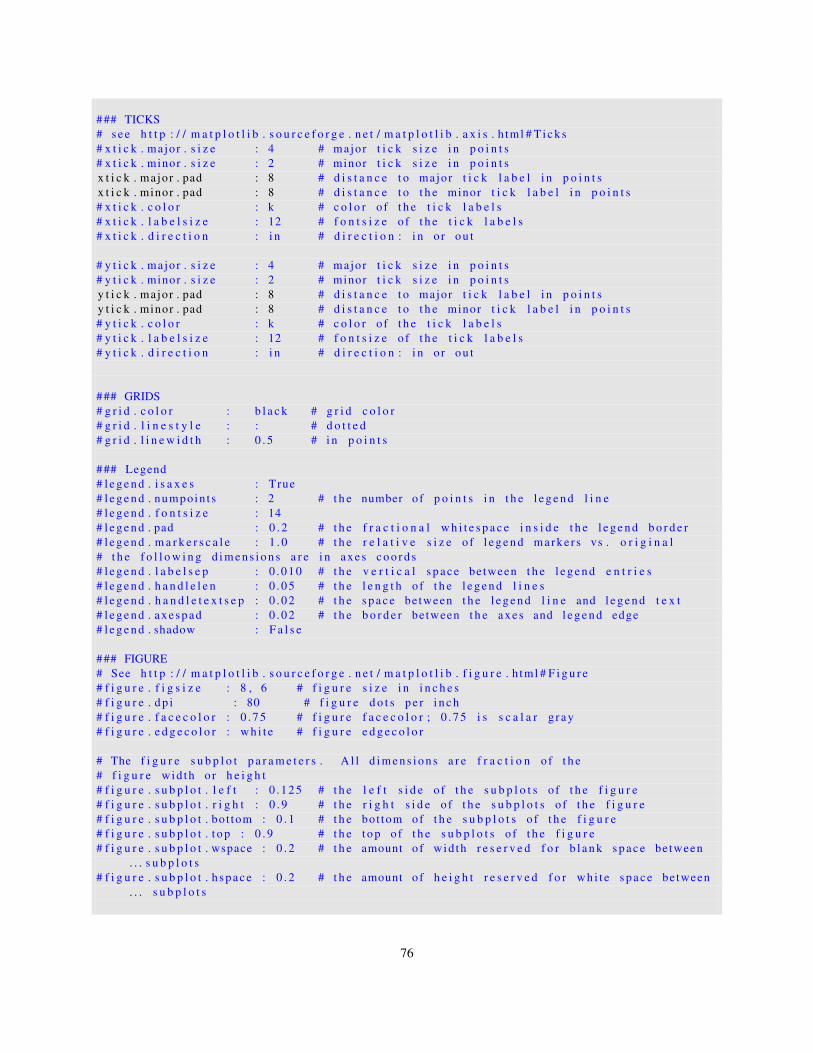
### TICKS# s e e h t t p : / / m a t p l o t l i b . s o u r c e f o r g e . n e t / m a t p l o t l i b . a x i s . h tml # T i c k s# x t i c k . major . s i z e : 4 # major t i c k s i z e i n p o i n t s# x t i c k . minor . s i z e : 2 # minor t i c k s i z e i n p o i n t sx t i c k . major . pad : 8 # d i s t a n c e t o major t i c k l a b e l i n p o i n t sx t i c k . minor . pad : 8 # d i s t a n c e t o t h e minor t i c k l a b e l i n p o i n t s# x t i c k . c o l o r : k # c o l o r o f t h e t i c k l a b e l s# x t i c k . l a b e l s i z e : 12 # f o n t s i z e o f t h e t i c k l a b e l s# x t i c k . d i r e c t i o n : i n # d i r e c t i o n : i n o r o u t

# y t i c k . major . s i z e : 4 # major t i c k s i z e i n p o i n t s# y t i c k . minor . s i z e : 2 # minor t i c k s i z e i n p o i n t sy t i c k . major . pad : 8 # d i s t a n c e t o major t i c k l a b e l i n p o i n t sy t i c k . minor . pad : 8 # d i s t a n c e t o t h e minor t i c k l a b e l i n p o i n t s# y t i c k . c o l o r : k # c o l o r o f t h e t i c k l a b e l s# y t i c k . l a b e l s i z e : 12 # f o n t s i z e o f t h e t i c k l a b e l s# y t i c k . d i r e c t i o n : i n # d i r e c t i o n : i n o r o u t

### GRIDS# g r i d . c o l o r : b l a c k # g r i d c o l o r# g r i d . l i n e s t y l e : : # d o t t e d# g r i d . l i n e w i d t h : 0 . 5 # i n p o i n t s

### Legend# l e g e n d . i s a x e s : True# l e g e n d . numpoin t s : 2 # t h e number o f p o i n t s i n t h e l e g e n d l i n e# l e g e n d . f o n t s i z e : 14# l e g e n d . pad : 0 . 2 # t h e f r a c t i o n a l w h i t e s p a c e i n s i d e t h e l e g e n d b o r d e r# l e g e n d . m a r k e r s c a l e : 1 . 0 # t h e r e l a t i v e s i z e o f l e g e n d marke r s vs . o r i g i n a l# t h e f o l l o w i n g d i m e n s i o n s a r e i n axes c o o r d s# l e g e n d . l a b e l s e p : 0 .010 # t h e v e r t i c a l s p a c e between t h e l e g e n d e n t r i e s# l e g e n d . h a n d l e l e n : 0 . 0 5 # t h e l e n g t h o f t h e l e g e n d l i n e s# l e g e n d . h a n d l e t e x t s e p : 0 . 0 2 # t h e s p a c e between t h e l e g e n d l i n e and l e g e n d t e x t# l e g e n d . axespad : 0 . 0 2 # t h e b o r d e r between t h e axes and l e g e n d edge# l e g e n d . shadow : F a l s e

### FIGURE# See h t t p : / / m a t p l o t l i b . s o u r c e f o r g e . n e t / m a t p l o t l i b . f i g u r e . h tml # F i g u r e# f i g u r e . f i g s i z e : 8 , 6 # f i g u r e s i z e i n i n c h e s# f i g u r e . d p i : 80 # f i g u r e d o t s p e r i n c h# f i g u r e . f a c e c o l o r : 0 . 7 5 # f i g u r e f a c e c o l o r ; 0 . 7 5 i s s c a l a r g ray# f i g u r e . e d g e c o l o r : w h i t e # f i g u r e e d g e c o l o r

# The f i g u r e s u b p l o t p a r a m e t e r s . A l l d i m e n s i o n s a r e f r a c t i o n o f t h e# f i g u r e wid th o r h e i g h t# f i g u r e . s u b p l o t . l e f t : 0 . 125 # t h e l e f t s i d e o f t h e s u b p l o t s o f t h e f i g u r e# f i g u r e . s u b p l o t . r i g h t : 0 . 9 # t h e r i g h t s i d e o f t h e s u b p l o t s o f t h e f i g u r e# f i g u r e . s u b p l o t . bo t tom : 0 . 1 # t h e bot tom of t h e s u b p l o t s o f t h e f i g u r e# f i g u r e . s u b p l o t . t o p : 0 . 9 # t h e t o p of t h e s u b p l o t s o f t h e f i g u r e# f i g u r e . s u b p l o t . wspace : 0 . 2 # t h e amount o f wid th r e s e r v e d f o r b l a n k s p a c e between

. . . s u b p l o t s# f i g u r e . s u b p l o t . h sp ac e : 0 . 2 # t h e amount o f h e i g h t r e s e r v e d f o r w h i t e s p a c e between

. . . s u b p l o t s

76

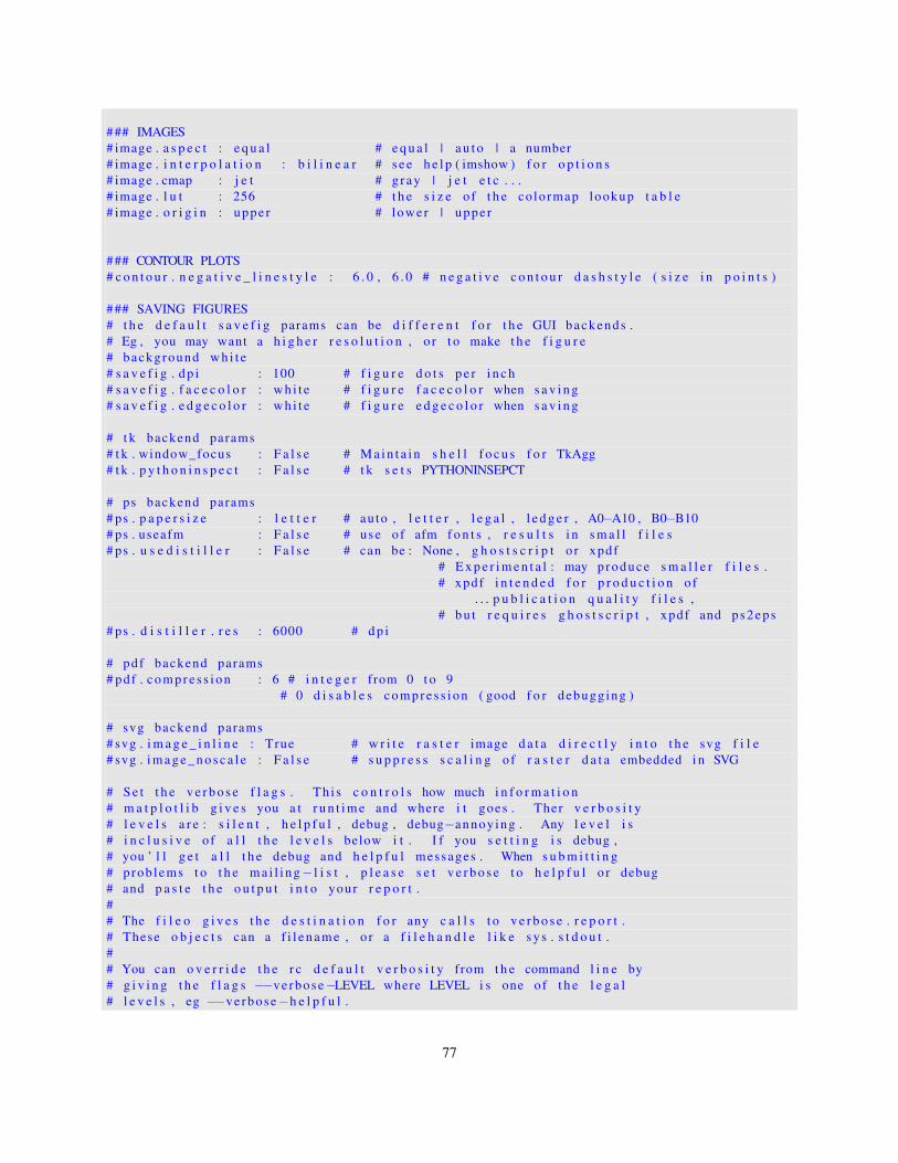
### IMAGES# image . a s p e c t : e q u a l # e q u a l | a u t o | a number# image . i n t e r p o l a t i o n : b i l i n e a r # s e e h e l p ( imshow ) f o r o p t i o n s# image . cmap : j e t # g ray | j e t e t c . . .# image . l u t : 256 # t h e s i z e o f t h e co lormap lookup t a b l e# image . o r i g i n : uppe r # lower | uppe r

### CONTOUR PLOTS# c o n t o u r . n e g a t i v e _ l i n e s t y l e : 6 . 0 , 6 . 0 # n e g a t i v e c o n t o u r d a s h s t y l e ( s i z e i n p o i n t s )

### SAVING FIGURES# t h e d e f a u l t s a v e f i g params can be d i f f e r e n t f o r t h e GUI backends .# Eg , you may want a h i g h e r r e s o l u t i o n , o r t o make t h e f i g u r e# background w h i t e# s a v e f i g . d p i : 100 # f i g u r e d o t s p e r i n c h# s a v e f i g . f a c e c o l o r : w h i t e # f i g u r e f a c e c o l o r when s a v i n g# s a v e f i g . e d g e c o l o r : w h i t e # f i g u r e e d g e c o l o r when s a v i n g

# t k backend params# t k . window_focus : F a l s e # M a i n t a i n s h e l l f o c u s f o r TkAgg# t k . p y t h o n i n s p e c t : F a l s e # t k s e t s PYTHONINSEPCT

# ps backend params# ps . p a p e r s i z e : l e t t e r # au to , l e t t e r , l e g a l , l e d g e r , A0−A10 , B0−B10# ps . useafm : F a l s e # use o f afm f o n t s , r e s u l t s i n s m a l l f i l e s# ps . u s e d i s t i l l e r : F a l s e # can be : None , g h o s t s c r i p t o r xpdf

# E x p e r i m e n t a l : may produce s m a l l e r f i l e s .# xpdf i n t e n d e d f o r p r o d u c t i o n o f

. . . p u b l i c a t i o n q u a l i t y f i l e s ,# b u t r e q u i r e s g h o s t s c r i p t , xpdf and ps 2e ps

# ps . d i s t i l l e r . r e s : 6000 # d p i

# pdf backend params# pdf . c o m p r e s s i o n : 6 # i n t e g e r from 0 t o 9

# 0 d i s a b l e s c o m p r e s s i o n ( good f o r debugg ing )

# svg backend params# svg . i m a g e _ i n l i n e : True # w r i t e r a s t e r image d a t a d i r e c t l y i n t o t h e svg f i l e# svg . i m a g e _ n o s c a l e : F a l s e # s u p p r e s s s c a l i n g o f r a s t e r d a t a embedded i n SVG

# S e t t h e v e r b o s e f l a g s . Th i s c o n t r o l s how much i n f o r m a t i o n# m a t p l o t l i b g i v e s you a t r u n t i m e and where i t goes . Ther v e r b o s i t y# l e v e l s a r e : s i l e n t , h e l p f u l , debug , debug−annoy ing . Any l e v e l i s# i n c l u s i v e o f a l l t h e l e v e l s below i t . I f you s e t t i n g i s debug ,# you ’ l l g e t a l l t h e debug and h e l p f u l messages . When s u b m i t t i n g# prob lems t o t h e m a i l i n g− l i s t , p l e a s e s e t v e r b o s e t o h e l p f u l o r debug# and p a s t e t h e o u t p u t i n t o your r e p o r t .## The f i l e o g i v e s t h e d e s t i n a t i o n f o r any c a l l s t o v e r b o s e . r e p o r t .# These o b j e c t s can a f i l e n a m e , o r a f i l e h a n d l e l i k e s y s . s t d o u t .## You can o v e r r i d e t h e r c d e f a u l t v e r b o s i t y from t h e command l i n e by# g i v i n g t h e f l a g s −−ve rbose−LEVEL where LEVEL i s one of t h e l e g a l# l e v e l s , eg −−ve rbose−h e l p f u l .

77

## You can a c c e s s t h e v e r b o s e i n s t a n c e i n your code# from m a t p l o t l i b i m p o r t v e r b o s e .# v e r b o s e . l e v e l : s i l e n t # one of s i l e n t , h e l p f u l , debug , debug−annoy ing# v e r b o s e . f i l e o : s y s . s t d o u t # a l o g f i l e n a m e , s y s . s t d o u t o r s y s . s t d e r r

78

Appendix B

mathtext symbols

79

80

Appendix C

matplotlib source code license

matplotlib is distributed under the Python Software Foundation (PSF) license, which permits commercial and noncom-mercial free use and redistribution as long as the conditions below are met. The VERSION string below is replacedby the current matplotlib version number with each release.

LICENSE AGREEMENT FOR MATPLOTLIB VERSION--------------------------------------

1. This LICENSE AGREEMENT is between the John D. Hunter ("JDH"), and theIndividual or Organization ("Licensee") accessing and otherwise usingmatplotlib software in source or binary form and its associateddocumentation.

2. Subject to the terms and conditions of this License Agreement, JDHhereby grants Licensee a nonexclusive, royalty-free, world-wide licenseto reproduce, analyze, test, perform and/or display publicly, preparederivative works, distribute, and otherwise use matplotlib VERSIONalone or in any derivative version, provided, however, that JDH’sLicense Agreement and JDH’s notice of copyright, i.e., "Copyright (c)2002-2004 John D. Hunter; All Rights Reserved" are retained inmatplotlib VERSION alone or in any derivative version prepared byLicensee.

3. In the event Licensee prepares a derivative work that is based on orincorporates matplotlib VERSION or any part thereof, and wants tomake the derivative work available to others as provided herein, thenLicensee hereby agrees to include in any such work a brief summary ofthe changes made to matplotlib VERSION.

4. JDH is making matplotlib VERSION available to Licensee on an "ASIS" basis. JDH MAKES NO REPRESENTATIONS OR WARRANTIES, EXPRESS ORIMPLIED. BY WAY OF EXAMPLE, BUT NOT LIMITATION, JDH MAKES NO ANDDISCLAIMS ANY REPRESENTATION OR WARRANTY OF MERCHANTABILITY OR FITNESSFOR ANY PARTICULAR PURPOSE OR THAT THE USE OF MATPLOTLIB VERSIONWILL NOT INFRINGE ANY THIRD PARTY RIGHTS.

5. JDH SHALL NOT BE LIABLE TO LICENSEE OR ANY OTHER USERS OF MATPLOTLIBVERSION FOR ANY INCIDENTAL, SPECIAL, OR CONSEQUENTIAL DAMAGES ORLOSS AS A RESULT OF MODIFYING, DISTRIBUTING, OR OTHERWISE USING

81

MATPLOTLIB VERSION, OR ANY DERIVATIVE THEREOF, EVEN IF ADVISED OFTHE POSSIBILITY THEREOF.

6. This License Agreement will automatically terminate upon a materialbreach of its terms and conditions.

7. Nothing in this License Agreement shall be deemed to create anyrelationship of agency, partnership, or joint venture between JDH andLicensee. This License Agreement does not grant permission to use JDHtrademarks or trade name in a trademark sense to endorse or promoteproducts or services of Licensee, or any third party.

8. By copying, installing or otherwise using matplotlib VERSION,Licensee agrees to be bound by the terms and conditions of this LicenseAgreement.

82

Bibliography

Julius S. Bendat and Allan G. Piersol. Random Data: Analysis and Measurement Procedures. John Wiley & Sons,New York, 1986.

Eric W. Weisstein. CRC Concise Encyclopedia of Mathematics. Chapman & Hall/CRC, second edition edition, 2002.

83