
The mathematics behind Computertomography - tu …bernstei/Tomo/Radontr.pdf · The mathematics...
54
Radon transforms The mathematics behind Computertomography PD Dr. Swanhild Bernstein, Institute of Applied Analysis, Freiberg University of Mining and Technology, International Summer academic course 2008, „Modelling and Simulation of Technical Processes“
Transcript of The mathematics behind Computertomography - tu …bernstei/Tomo/Radontr.pdf · The mathematics...

Radon transformsThe mathematics behind ComputertomographyPD Dr. Swanhild Bernstein, Institute of Applied Analysis,
Freiberg University of Mining and Technology,
International Summer academic course 2008,
„Modelling and Simulation of Technical Processes“

Historical remarks
C. Röntgen (1895) – X-rays
J. Radon (1917)– Mathematical Model
G. Grossmann (1935) – Tomography
G. Hounsfield, McCormack (1972) –Computerized assited tomography (CAT scan)
Why does it work?The physical priniples.
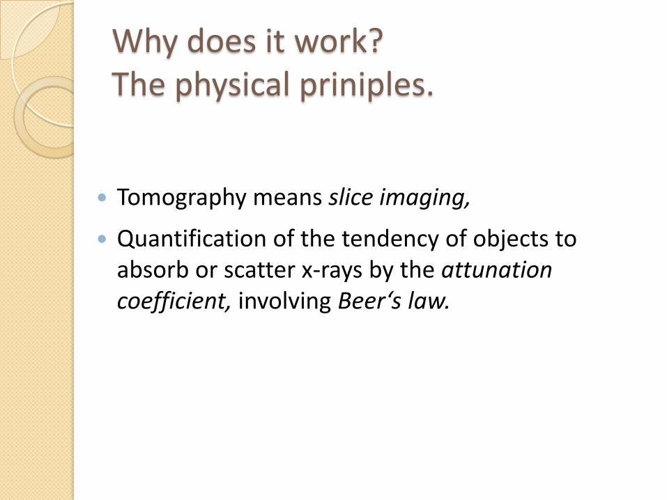
Tomography means slice imaging,
Quantification of the tendency of objects toabsorb or scatter x-rays by the attunationcoefficient, involving Beer‘s law.
Model
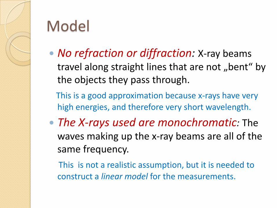
No refraction or diffraction: X-ray beamstravel along straight lines that are not „bent“ bythe objects they pass through.
This is a good approximation because x-rays have veryhigh energies, and therefore very short wavelength.
The X-rays used are monochromatic: The waves making up the x-ray beams are all of thesame frequency.
This is not a realistic assumption, but it is needed toconstruct a linear model for the measurements.

Beer‘s law: Each material encountered has a characteristic linear attenuation coefficient μfor x-rays of a given energy.
The intensity, I of the x-ray beam satisfies Beer‘slaw:
Here, s is the arc-length along the straight line
trajectory of the x-ray beam.
Model
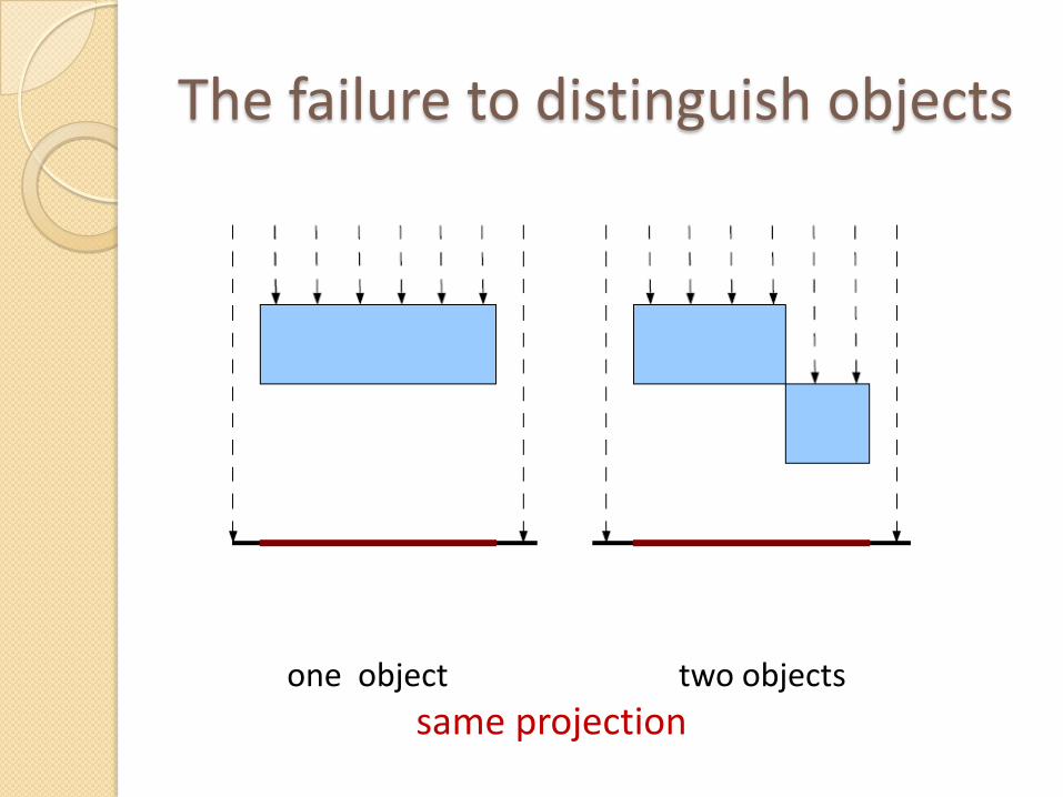
The failure to distinguish objects
one object two objects
same projection

Solution: more directions
Different angles lead to different projections. The more directions from which we makemeasurement, the more arrangements of objectswe can distinguish.

Analysis of a Point Source Device,2D model, what do we measure?

2D model, what do we measure?
Beer‘s law:
First order ordinary differential equation for theintensity I with boundary condition I at r=r0>0 equals I0.
Ex 1

2D model, what do we measure?
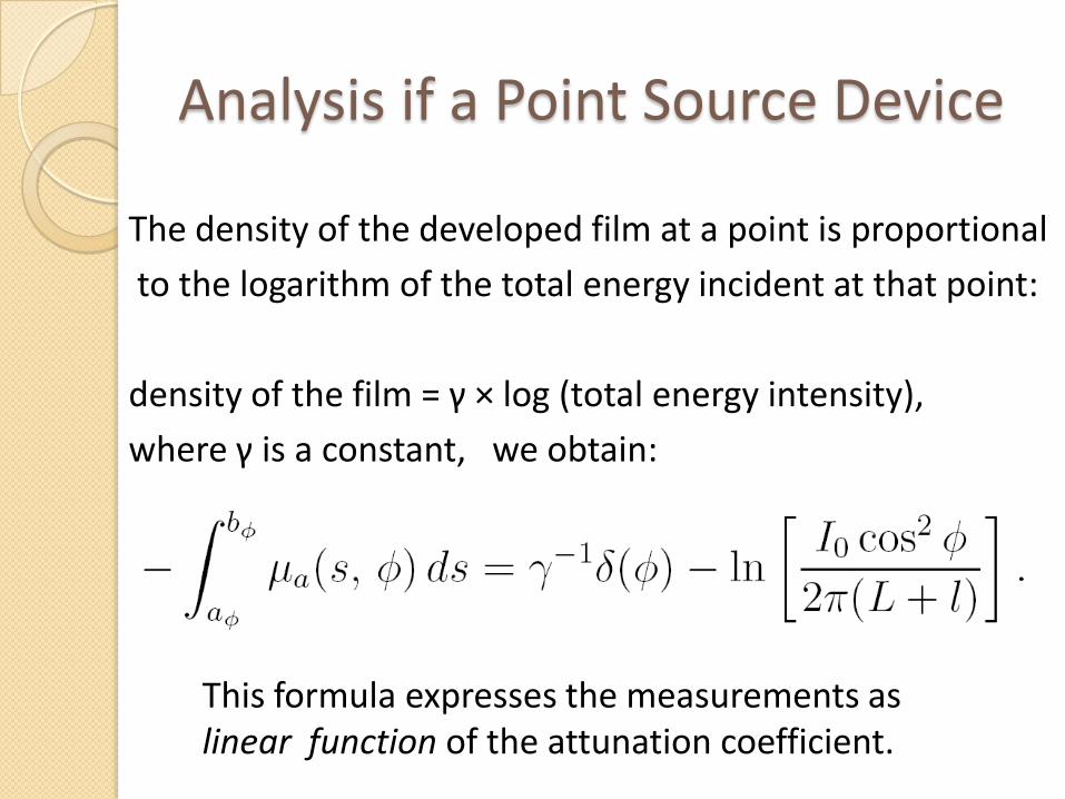
Analysis if a Point Source Device
The density of the developed film at a point is proportional
to the logarithm of the total energy incident at that point:
density of the film = γ × log (total energy intensity),
where γ is a constant, we obtain:
This formula expresses the measurements aslinear function of the attunation coefficient.

Oriented lines
t
t is the distant of the line from the origin,s is the parameter of the line.

Radon transform

Radon transform

Radon transform
The Radon transform can be defined, a priori for a function, f whose restriction to each line is locally integrable and
This is really two different conditions:1. The function is regular enough so that restricting it to any
line gives a locally integrable function,2. The function goes to zero rapidly enough for the improper
integrals to converge.
In applications functions of interest are usually piecewisecontinuous and zero outside of some disk.
Ex 2

Properties of the Radon transform
The Radon transform is linear:
The Radon transform of f is an even function:
The Radon transform is monotone: if f is a non-negative function then

Pencilgeometry (Nadelstrahlgeometrie)
Buzug, Einführung in die Computertomography, Springer Verlag , 2004

Back-projection formula
It is difficult to use the line integrals of a functiondirectly to reconstruct the function:
Results of the recontruction by back-projection
What is that??
Buzug, Einführung in die Computertomography, Springer Verlag , 2004

Fourier transform in 1D The Fourier transform of an absolutely integrable
function f, defined on the real line, is
Suppose that the Fourier transform of f is again an absolutely integrable function then

Square integrable functions
Ex 3
A (complex-valued) function f, defined on , is squareintegrable if
Examples: The function is not absolutely integrable but square integrable, thefunction
is absolutely integrable but not square integrable.
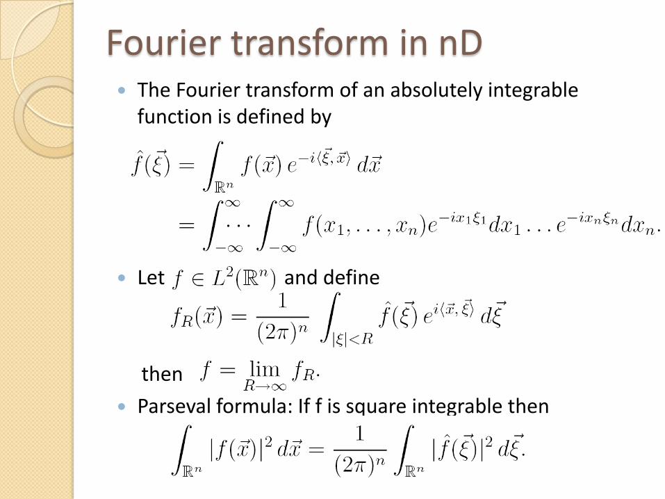
Fourier transform in nD The Fourier transform of an absolutely integrable
function is defined by
Let and define
then
Parseval formula: If f is square integrable then

Let f be an absolutely integrable function. For any real number r and unit vector , we have the identity
For a given vector the inner product ,
is constant along any line perpendicular to the direction
. The central slice theorem interprets the computionof the Fourier transform of as a two-step process:
1. First, integrate the function along lines perp. to .
2. Compute the one-dimensional Fourier transform ofthis function of the affine parameter.
Central Slice Theorem
Ex 4

Inverse Radon Transform andCentral Slice Theorem
3. Compute the one dimensional Fourier transform of
1. Choose a line L, determinedby the direction (Cartesiancoord.) or by the angle γ .Then the coorinate axis ξ showsin the same direction.
2. Integrate along all lines perp.to (those lines are parallelto the cood. axis η. We obtainthe Radon transform .
4. With u=q cos γ and v=q sin γ,we get F(u,v) = andf(x,y) is equal to the 2D inverseFourier transform of F(u,v).
Buzug, Einführung in die Computertomography, Springer Verlag , 2004

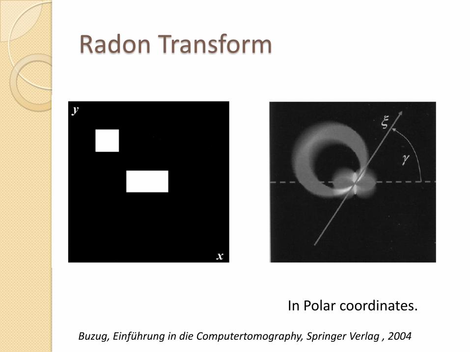
Radon Transform
Buzug, Einführung in die Computertomography, Springer Verlag , 2004

Radon Transform
In Cartesian coordinates.
Buzug, Einführung in die Computertomography, Springer Verlag , 2004
Radon Transform
In Polar coordinates.
Buzug, Einführung in die Computertomography, Springer Verlag , 2004

Radon Transform
Abdomen, Radon transform in Cartesian coord.
Buzug, Einführung in die Computertomography, Springer Verlag , 2004
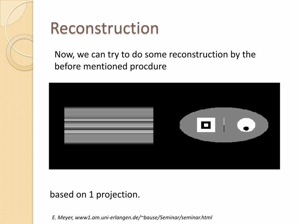
Reconstruction
based on 1 projection.
Now, we can try to do some reconstruction by thebefore mentioned procdure
E. Meyer, www1.am.uni-erlangen.de/~bause/Seminar/seminar.html

based on 4 projections.
Reconstruction
E. Meyer, www1.am.uni-erlangen.de/~bause/Seminar/seminar.html

based on 8 projections.
Reconstruction
E. Meyer, www1.am.uni-erlangen.de/~bause/Seminar/seminar.html

based on 30 projections.
Reconstruction
E. Meyer, www1.am.uni-erlangen.de/~bause/Seminar/seminar.html

based on 60 projections.
Reconstruction
What is the difference to the back-projection formula?
E. Meyer, www1.am.uni-erlangen.de/~bause/Seminar/seminar.html

Radon Inversion Formula
If f is an absolutely integrable function and ist Fourier transform is absolutely integrable too, then

Radon Inversion Formula If f is an absolutely integrable function and its Fourier
transform is absolutely integrable too, then
Filtered Back-Projection
1. The radial integral is interpreted as a filter applied tothe Radon transform. The filter acts only the affine parameter; is output of the filter is denoted
2. The angular integral is then interpreted as the back-projection of the filtered Radon transform.
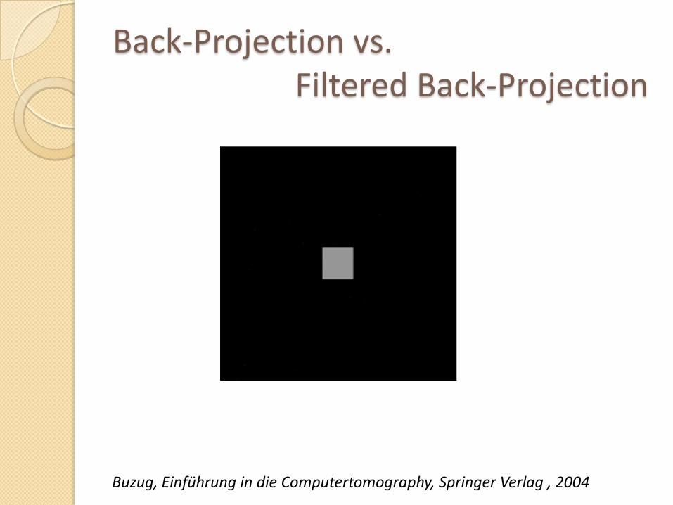
Back-Projection vs. Filtered Back-Projection
Buzug, Einführung in die Computertomography, Springer Verlag , 2004
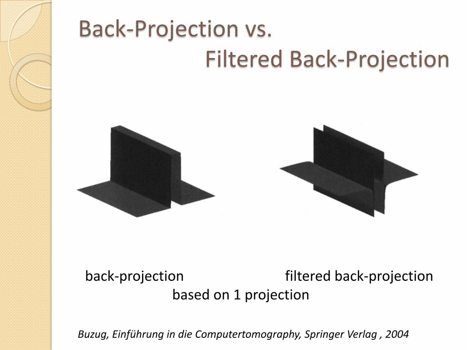
Back-Projection vs. Filtered Back-Projection
back-projection filtered back-projectionbased on 1 projection
Buzug, Einführung in die Computertomography, Springer Verlag , 2004
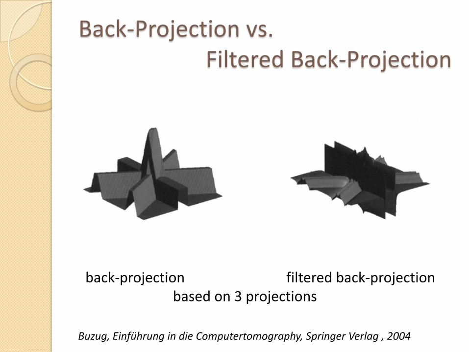
Back-Projection vs. Filtered Back-Projection
back-projection filtered back-projectionbased on 3 projections
Buzug, Einführung in die Computertomography, Springer Verlag , 2004
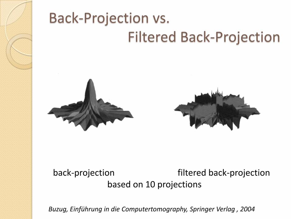
Back-Projection vs. Filtered Back-Projection
back-projection filtered back-projectionbased on 10 projections
Buzug, Einführung in die Computertomography, Springer Verlag , 2004
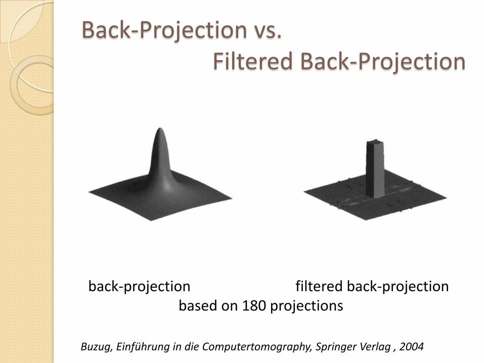
Back-Projection vs. Filtered Back-Projection
back-projection filtered back-projectionbased on 180 projections
Buzug, Einführung in die Computertomography, Springer Verlag , 2004

Back-Projection vs. Filtered Back-Projection
back-projection filtered back-projectionbased on 180 projections
Buzug, Einführung in die Computertomography, Springer Verlag , 2004

Back-Projection vs. Filtered Back-Projection
a) back-projection and b) filtered back-projection,based on 1, 2, 3, 10, 45 projections resp.
Buzug, Einführung in die Computertomography, Springer Verlag , 2004

Different Inversion formulas
We already had the Radon inversion formula:
We write |r| as sgn(r) r :

A Different Inversion formula We already had the Radon inversion formula:
Where we write |r|as sgn(r) r
denotes the 1D Fourier
transform with respect to t.
Suppose that g is square integrable on the real line. The
Hilbert transform of g is defined by
If is also absolutely integrable, then
We obtain

Mathematical Model for CT We consider a two-dimensional slice of an three-dimensional
object, the physical parameters of interest is the attenuationcoefficient f of the two-dimensional slice. According to Beer‘slaw, the intensity traveling along a line is attenuated accordingto the differential equation
where s is arclength along the line.
By comparing the intensity of an incident beam of x-rays to thatemitted, we measure the Radon transform of f:
Using the Radon inversion formula, the attenuation coefficient f is reconstructed from the measurements
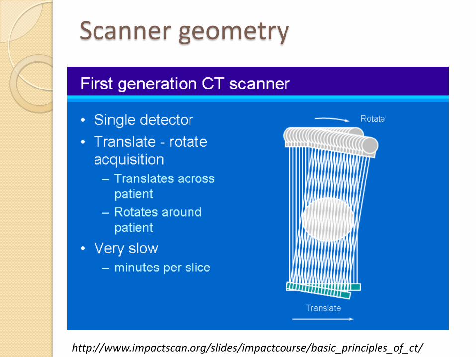
Scanner geometry
http://www.impactscan.org/slides/impactcourse/basic_principles_of_ct/
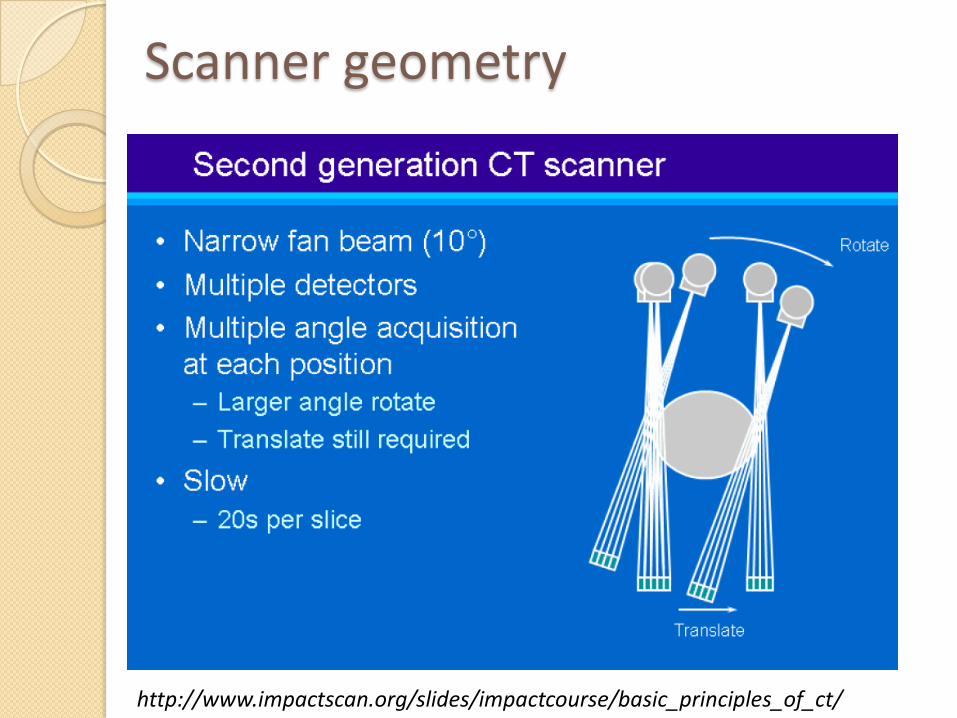
Scanner geometry
http://www.impactscan.org/slides/impactcourse/basic_principles_of_ct/

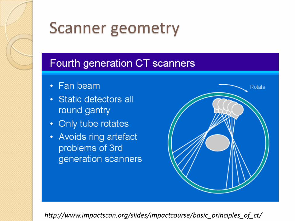
Scanner geometry
http://www.impactscan.org/slides/impactcourse/basic_principles_of_ct/
Scanner geometry
http://www.impactscan.org/slides/impactcourse/basic_principles_of_ct/

Radon transform - Polar gridFourier transform – Cartesian grid
Buzug, Einführung in die Computertomography, Springer Verlag , 2004

Why fan beam?
http://www.impactscan.org/slides/impactcourse/basic_principles_of_ct/
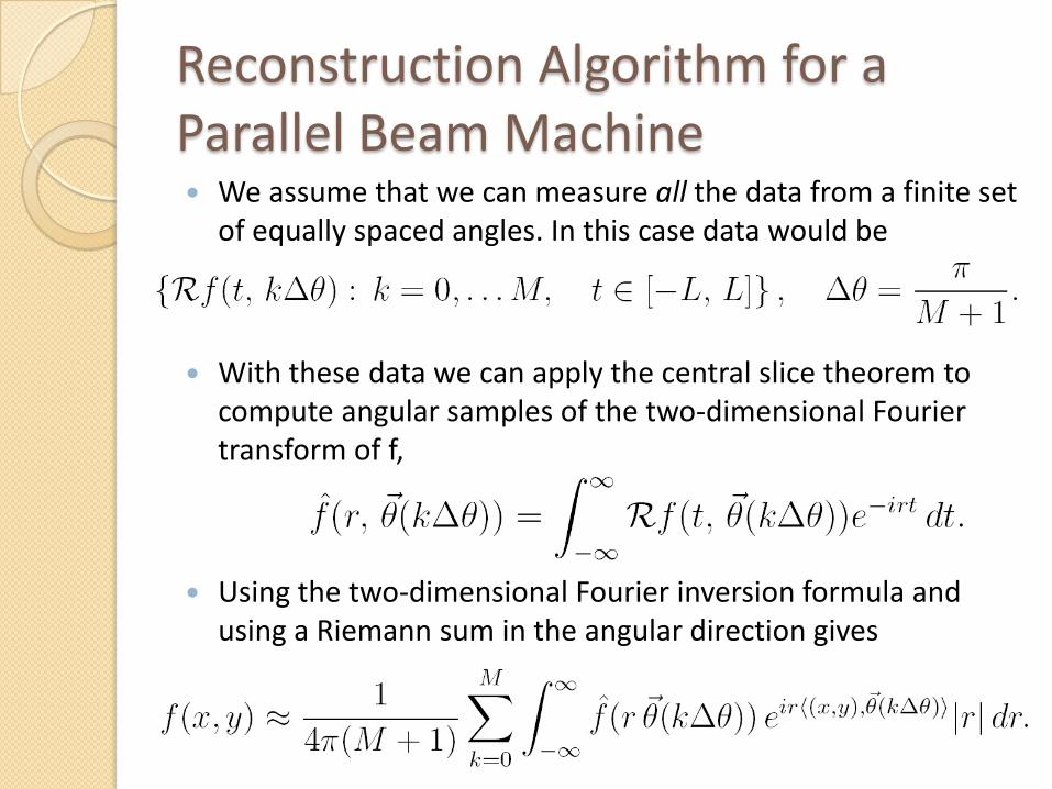
Reconstruction Algorithm for a Parallel Beam Machine We assume that we can measure all the data from a finite set
of equally spaced angles. In this case data would be
With these data we can apply the central slice theorem tocompute angular samples of the two-dimensional Fourier transform of f,
Using the two-dimensional Fourier inversion formula andusing a Riemann sum in the angular direction gives

Concluding remarks
The model present here is a CT-model, there exist othertypes of tomographical methods that are based on other mathematical models.
All mathematical models are based on so-called integral geometry and connected with wave equations.
Modern tomography even combines different methods:
fusion of CT-scan (grey)
and PET-scan (grey)
PET = Positron Emission
Tomography
http://www.sdirad.com/PatientInfo/pt_pet.htm

Most of the pictures are dealing with medical applications
but Computer tomography can be applied to more
applications, as for example:
Material sciencesTomographic visualisation of a metallic foam structure
http://www2.tu-berlin.de/fak3/sem/GB_index.html
Geologyhttp://www.geo.cornell.edu/geology/classes/Geo101/
101images_spring.html
Seismic tomography reveals a more
complex interior structure.
Archeology3D-Computer Tomography of
Prehispanic Sound Artifacts.
Supported by the Ethnological Museum Berlin and the St. Gertrauden Hospital, Berlin.
http://www.mixcoacalli.com/wp-content/uploads/2007/09/ct2.jpg
Concluding remarks

Bibliography
Charles L. Epstein, Introduction to the Mathematics ofMedical Imaging, Pearson Education, Inc., 2003
Thorsten M. Buzug, Einführung in die Computertomographie, Springer Verlag, 2004
Esther Meyer, Die Mathematik der Computertomogrphie, Seminarvortrag, www1.am.unierlangen.de/~bause/Seminar/seminar.html
Other pictures are fromwww.impactscan.org/slides/impactcourse/basic_principles_of_ct/
www.sdirad.com/PatientInfo/pt_pet.htm


