The macroeconomics of rational bubbles: a user’s guide

Alberto Martin and Jaume Ventura∗

February 2018

Abstract

This paper provides a guide to macroeconomic applications of the theory of rational bubbles.

It shows that rational bubbles can be easily incorporated into standard macroeconomic models,

and illustrates how they can be used to account for important macroeconomic phenomena. It also

discusses the welfare implications of rational bubbles and the role of policy in managing them.

Finally, it provides a detailed review of the literature.

JEL classification: E32, E44, O40

Keywords: bubbles, credit, business cycles, economic growth, financial frictions, pyramid schemes

∗Martin: amartin@crei.cat. Ventura: jventura@crei.cat. All authors: CREI, Universitat Pompeu Fabra and Bar-

celona GSE, Ramon Trias Fargas 25-27, 08005-Barcelona, Spain. We are grateful to Oscar Arce, Vladimir Asriyan,

Gadi Barlevy, Sergi Basco, Gene Grossman, Jian Jun Miao and Toan Phan for their comments on an earlier draft.

We also thank Joon Sup Park for pointing out an algebra mistake on an earlier draft. Janko Heineken and Ilja

Kantorovitch for provided superb research assistance. Martin acknowledges support from the Spanish Ministry of

Economy, Industry and Competitiveness (grant ECO2016-79823-P) and from the ERC (Consolidator Grant FP7-

615651–MacroColl). Ventura acknowledges support from the Spanish Ministry of Economy and Competitiveness

(grant ECO2014-54430-P) and from the ERC Horizon 2020 Research and Innovation Programme (grant agreement

693512). In addition, both authors acknowledge support from the Spanish Ministry of Economy and Competitive-

ness, through the Severo Ochoa Programme for Centres of Excellence in R&D (SEV-2015-0563), from the CERCA

Programme/Generalitat de Catalunya, from the Generalitat de Catalunya (grant 2014SGR-830 AGAUR), and from

the Barcelona GSE Research Network.

Recent decades have been characterized by large swings in asset prices. To illustrate this, the

top panels of Figures 1-4 depict the ratio of household net worth to GDP in Japan, the United

States, Spain and Ireland at different times over the last three decades. Loosely speaking, this ratio

captures the value of all assets in an economy and its evolution largely mirrors the behavior of real

estate and stock prices. As the figures shows, all of these countries have experienced episodes of

large increases in asset prices – entailing a creation of wealth of one GDP or more – followed by

sharp declines.

Besides their direct effect on household wealth, these fluctuations in asset prices have had

profound macroeconomic implications. This is illustrated in the middle and bottom panels of

Figures 1-4, which respectively depict the current account balance and the growth rates of output,

consumption, and the capital stock. There are two main messages from these panels. First, large

asset price booms were in most instances accompanied by large capital inflows, and their collapse

by sharp reversals in capital flows. Second, asset price booms were often accompanied by large

upswings in real activity – as measured by the growth rates of output, consumption and the capital

stock – and their collapse by economic busts. Indeed, most boom-bust episodes ended in economic

recessions, as depicted by the shaded bars in Figures 1-4.

In light of these developments, macroeconomists have felt the need to develop new models to

understand what drives these large swings in asset prices and how do they affect the macroeconomy.

We review here one class of models that rely on two simple premises or working hypotheses. The

first one is that asset prices are not only driven by fundamentals, but also by bubbles that respond to

random and capricious shifts in market psychology. The second hypothesis is that these bubbles are

consistent with individual rationality. In fact, shifts in market psychology can be easily incorporated

into standard macroeconomic models that rely on rational expectations, individual maximization,

and market clearing.

These two hypotheses define the research on the macroeconomics of rational bubbles. The

key words are macroeconomic and rational. Macroeconomic in the sense that this research is not

interested in explaining the causes and effects of pricing anomalies or pathologies in some specific

market, e.g. tulips, but rather in understanding large, widespread fluctuations in asset prices in

modern economies. Rational in the sense that one of its key insights is that there are multiple

market psychologies that are consistent with individual rationality. Whereas macroeconomists

typically focus on one such psychology, i.e., asset prices are equal to the fundamental, there is no

compelling reason to do so. Other psychologies may provide a more natural account of important

1

macroeconomic phenomena.

Two caveats are in order. The first is that this is a user’s guide, which is defined by the Oxford

English Dictionary as “a handbook containing instructions on how to use a device”. As such, it is

more technical than the usual survey or literature review. We want to tell readers what bubbles

do, but we also want to show them how and why. We do so through a series of simple models and

examples.

A second caveat is that this guide reflects our personal views, which have evolved over more than

a decade of working on the topic. Because of this, it draws heavily from our own research and reflects

our general narrative. Needless to say, many other researchers have contributed substantially to the

topic. We acknowledge this in a detailed literature review that explains how this line of research

has evolved and how the different contributions relate to each other.

The rest of the paper is organized as follows. Section 1 uses a small open economy model to show

how bubbles generate fluctuations in capital flows, investment, and output. This partial-equilibrium

framework allows us to identify and analyze some of the most important macroeconomic effects

of bubbles. Section 2 extends the analysis to a world economy model. This general-equilibrium

setting enables us to analyze the conditions for the existence of bubbles. It also allows us to explore

the interaction between financial globalization and bubbles, and to derive the welfare and policy

implications of bubbles. Section 3 contains the literature review. Finally, section 4 provides a brief

discussion of the main challenges that this research program is facing.

1 Bubbly boom-bust cycles

The popular notion of a bubble or bubbly episode refers to a situation in which, for no really good

reason, asset values and credit start growing rapidly. This marks the beginning of a period in which

investment expands sharply, typically financed by large capital inflows. Output and consumption

growth accelerate. Some of the new investments might seem unproductive, especially if they are

made in low productivity sectors such as real estate. But this is not perceived to be a major problem

contemporaneously. After all, the population enjoys a high level of consumption and well-being.

Eventually, again for no really good reason, asset values and credit drop, often quite dramati-

cally. This leads to a sudden collapse in investment and a reversal of capital flows. Output and

consumption growth stop abruptly and might even turn negative. Some of the investments made

during the expansionary phase turn out to have little value, and they might even be abandoned or

2

dismantled. The population now suffers a low level of consumption and well-being.

This is the stylized view of bubbly boom-bust cycles held by many economic analysts and

policymakers around the world, and it is based on experiences such as those shown in Figures 1-4.

Perhaps the most defining aspect of this view is that movements in asset values and credit do not

seem to be justified by major changes in economic conditions. Instead, they seem to be driven by

random and capricious shifts in market psychology. Another important aspect of this view is that

even in those cases in which investments are mostly unproductive or even useless, they still seem to

create value and raise wealth during the expansionary period. These aspects of bubbly episodes are

hard to generate in conventional macroeconomic models. But they are a central feature of models

of rational bubbles. Thus, a major selling point of the theory is that it can formalize this popular

view and make sense of it.

There is much more to the theory of rational bubbles than its ability to formalize this view, of

course. We shall show this amply here. But we have to start somewhere, and this constitutes an

excellent entry point to the macroeconomics of rational bubbles. Next, we construct this popular

view step by step, showing how each of the elements fits into a progressively more sophisticated and

nuanced story. To do this, we begin with a simple “lab economy” that provides a useful starting

point to explore the macroeconomic role of bubbles.

1.1 A simple lab economy

Imagine an economy that is only a very small part of a large world. This economy contains equal-

sized overlapping generations that live for two periods. All generations are endowed with one unit

of labor when young and their goal is to maximize expected consumption when old.1 Domestic

residents and foreigners interact in the credit market, where they exchange consumption goods

today for promises to deliver consumption goods in the future. Foreigners are willing to buy or

sell any credit contract that offers a gross expected return equal to R. We refer to R as the world

interest rate.

Production of consumption goods requires capital and labor, using a standard Cobb-Douglas

technology: Yt = A · Kαt ·(γt · Lt

)1−α; with A > 0, γ > 0 and α ∈ (0, 1); where Yt, Kt and Lt

denote output, the capital stock and the labor force, respectively. To produce one unit of capital for

period t+ 1, one unit of the final good is needed in period t. Capital depreciates at rate δ ∈ (0, 1),

1This assumption simplifies the analysis substantially since it implies that the young save all their income and use

it to construct portfolios with the highest possible expected return.

3

and it is reversible. The labor force is constant and equal to one. But labor productivity grows at

the rate γ ≥ 1. As usual we work with quantity variables expressed in efficiency units and denote

them with lowercase letters. For instance, we refer to kt as the capital stock, and we define it as

kt ≡ γ−t ·Kt.

Factor markets are competitive and factors earn their marginal product:

wt = (1− α) ·A · kαt (1)

rt = α ·A · kα−1t (2)

where wt and rt are the wage per effective worker and the rental per effective unit of capital,

respectively.

We make two assumptions throughout. All capital is owned by domestic firms, which receive

the capital income. All domestic firms are owned by domestic residents, who buy old firms and

create new ones at zero cost.2 Let vt be the market value of all firms after the rental has been

distributed to firm owners, but before new investments have been made. These firms own all the

undepreciated capital left after production, i.e. (1− δ) · kt. We think of vt as the value of all assets

contained in the country, that is, the theoretical counterpart of the net worth data shown in Figures

1-4.

Domestic residents may want to borrow from foreigners to purchase firms and to invest. We

introduce a friction that limits borrowing, though. Domestic courts can only seize the assets of

domestic residents, i.e., their firms, but not the rental income of capital. One interpretation of this

assumption is that the rental income can be “hidden” by domestic residents from the courts. As

a result, the young can only promise a payment of vt+1 to their creditors. Let ft be borrowing

or credit. Since contingent contracts are possible, young firm owners face the following borrowing

limit:3

R · ft ≤ γ · Etvt+1 (3)

where E denotes the expectation operator and we include it here because, as we shall see, v can

be stochastic. This borrowing limit links credit and asset values, and it is a key element of many

conventional macroeconomic models nowadays.

2This is an assumption about effective or ultimate control of assets. It does not preclude domestic firms to issue

and sell contingent credit contracts such as equity.3To implement this borrowing limit, entrepreneurs sell credit contracts that promise a contingent return equal to

Rt+1 =vt+1

Etvt+1·R. This contract maximizes promised payments in all possible histories.

4

Some readers might be wondering why our notation distinguishes between the price of firms and

the value of their capital. The reason, of course, is that bubbles create a wedge between these two

concepts, as we shall see shortly. But the overwhelming choice in current macroeconomic research

is to disregard this wedge and focus on equilibria in which these two quantities coincide:

vt = (1− δ) · kt (4)

If Equation (4) holds, we can write the maximization problem of the young as follows:

max γ · Etct+1 = (rt+1 + 1− δ) · γ · kt+1 −R · ft (5)

s. t. γ · kt+1 = wt + ft

R · ft ≤ (1− δ) · γ · kt+1

The young take the wage and rental as given and maximize expected old age consumption. The

latter equals the rental, i.e. rt+1·kt+1; plus the price obtained by selling their firms, i.e. (1− δ)·kt+1;

minus interest payments. This maximization is subject to two constraints. The first one is the

budget constraint, and it says that investment, i.e. γ·kt+1−(1− δ)·kt; plus the purchase of old firms,

i.e. (1− δ) · kt; must equal labor income plus borrowing. The second constraint is the borrowing

limit and it says that interest payments cannot exceed the value of firms, i.e. (1− δ) · γ · kt+1.

The choice variables in the maximization problem (5) are borrowing (ft) and the capital stock

(kt+1). If firms can costlessly merge or separate, or if they can buy and sell used capital, the concept

of firm becomes a veil. Choosing which specific firms to buy and create does not really matter.

The only thing that matters is how much capital is ultimately being held.

Maximization and market clearing imply that:

γ · kt+1 = min

{R

R+ δ − 1· (1− α) ·A · kαt , γ ·

(α ·A

R+ δ − 1

) 11−α}

(6)

Equation (6) is the law of motion of the capital stock and it contains two distinct regions. The

key variable that determines these regions is wealth, which here equals the wage of the young. If

kt weakly excceds a threshold k, wealth is high enough to ensure that the borrowing limit is not

binding.4 The young invest up to the point at which the return to capital equals the world interest

rate: rt+1 + 1− δ = R. If kt < k, wealth is too low and the borrowing limit is binding. The return

to capital exceeds the world interest rate: rt+1 + 1 − δ > R. As it is customary in models of the

4Formally, k =

[(α ·A

R+ δ − 1

) α1−α· γR· α

1− α

] 1α

.

5

financial accelerator type (of which this one is an example), when the borrowing limit binds the

capital stock is a multiple of wealth. This multiple is known as the financial multiplier since it

measures how many units of capital can be purchased for each unit of wealth. The intuition behind

this multiplier is well known. One additional unit of wealth allows the young to purchase one unit

of capital. This allows the young to borrow and raise the capital stock by1− δR

additional units.

And this allows them to borrow and raise the capital stock by

(1− δR

)2

additional units. And so

on. Thus, one unit of wealth allows the young to purchase 1 +1− δR

+

(1− δR

)2

+ ... =R

R+ δ − 1units of capital.

From any initial condition the capital stock monotonically converges to a unique steady state

kF . This convergence is fast if kt > k, but slow if kt < k. The borrowing limit is binding in the

steady state if the interest rate is low enough.5 These are definitely quiet dynamics. It might seem

that we have chosen the wrong economy to study the sort of messy and often dramatic events

that are associated with the popular view of bubbles. But events of this sort are lurking in the

background. To bring them to the fore, we just need to relax the assumption that firms are worth

the capital they own. There is no theoretical reason to keep this assumption, and there is much to

gain from relaxing it.

1.2 Building a theory of bubbly episodes

The theory of rational bubbles expands the set of equilibria under consideration. In particular, it

also considers equilibria in which the price of firms does not coincide with that of their capital:

vt = (1− δ) · kt + bt (7)

where bt is the bubble or bubble component of firm values. It is useful to think about this bubble

as the sum of bubbles attached to specific firms in the economy. Thus, the bubble has two sources

of dynamics: the growth of bubbles attached to old firms and the creation of new bubbles attached

to new firms. We can express this idea with the following notation:

γ · bt+1 = gt+1 · (bt + nt) (8)

Each period, the economy arrives with old bubbles bt attached to old firms. New firms are created

with new bubbles nt attached to them. Equation (8) recognizes that new bubbles in period t are

5In particular, if R < γ · α

1− α .

6

already old bubbles by period t+1, and it implicitly defines gt+1 as the growth rate of bubbles (old

and new) from period t to period t+ 1.

It is almost universally assumed that bubbles cannot be negative. This restriction is motivated

by appealing to some notion of free disposal. If a firm were to contain a negative bubble, the

argument goes, the owner could always start a new firm without bubble, transfer all the capital

from the old firm to it, and close the old firm. Naturally, there might be costs of opening/closing

firms and transferring capital among them. Or it might not be possible to start a new firm without

a bubble. We abstract from these complications and follow standard practice by assuming free

disposal of bubbles, i.e. bt ≥ 0 and nt ≥ 0.

Why do new bubbles pop up only in new firms? Is it possible that new bubbles pop up also in

old firms? Diba and Grossman (1988) argued that, if a firm contains a bubble, this bubble must

have started on the first date in which the firm was traded. Bubble creation after the first date of

trading would involve an innovation in the firm price. If markets are efficient, this innovation must

have had a zero expected value on the first date of trading. If there is free disposal of bubbles, this

innovation must be non-negative. Combining these two observations we reach the conclusion that

bubble creation must be exactly zero after the first date of trading. The Diba-Grossman argument

is sometimes invoked as a “proof” that bubbles cannot be created. This is obviously misleading,

since their argument does not impose any restriction on the size of new bubbles attached to new

firms. Moreover, one can also relax the assumptions of market efficiency and/or free disposal to

make it possible for new bubbles to pop up in old firms. To simplify the exposition, though, we

keep these two assumptions here.

As this discussion highlights, a key concept of the theory of rational bubbles is that of market

psychology. By this we mean a set of assumptions that define the bubble and its evolution. The

theory of rational bubbles is interested in the set of market psychologies that are consistent with

maximization and market clearing. Indeed, it is precisely the focus on this particular set that gives

the name to the theory. Sometimes, this set contains a unique market psychology.6 But usually the

set contains many market psychologies, and the modeler is forced to make a choice. This is the case

here. By choosing the specific market psychology that rules out bubbles, we obtained Equation (6)

and the quiet dynamics associated with it. What happens if we make another choice?

6If there is a unique rational market psychology, it is typically the one that rules out bubbles. But we know since

Tirole (1985) that there exist environments in which the unique rational market psychology must feature a bubble.

This case has been used recently by Allen, Barlevy and Gale (2017).

7

1.3 The wealth effect of new bubbles

We begin by considering a market psychology according to which the economy transits between

two states: zt ∈ {B,F}. During the bubbly state, new bubbles pop up with a combined size η > 0.

During the fundamental state, no new bubbles pop up. Let ϕ and ψ be the transition probabilities

from the bubbly to the fundamental state and vice-versa, respectively. With these assumptions,

we have that:

nt =

η if zt = B

0 if zt = F(9)

This is a stylized model of market psychology. Some periods investor sentiment is such that markets

are willing to finance investment on the basis of new bubbles. Some other periods, investor sentiment

is such that markets are unwilling to do so. The transition between these states is random and

unrelated to economic conditions.

Replacing Equation (4) with Equations (7) and (8), we can write the maximization problem of

the young as follows:

max γ · Etct+1 = (rt+1 + 1− δ) · γ · kt+1 + Etgt+1 · (xt · bt + nt)−R · ft (10)

s. t. γ · kt+1 + xt · bt = wt + ft

R · ft ≤ (1− δ) · γ · kt+1 + Etgt+1 · (xt · bt + nt) ,

where xt denotes bubble demand by the young as a share of the aggregate bubble. Now the

choice variables are borrowing (ft), the capital stock (kt+1) and the bubble demanded (xt). Bubble

creation nt is not a choice variable because, according to the market psychology of Equation (9),

it is exogenous. Once again, if firms can costlessly merge or separate, or if they can buy and sell

used capital, the concept of a firm becomes a veil. Choosing which specific firms to buy and create

does not really matter. The only thing that matters is how much capital and bubble are ultimately

being held.7

Individual maximization plus market clearing (xt = 1) implies,

Etgt+1 = R, (11)

7We are assuming here that mergers/separations and purchases/sales of capital do no affect the bubble component.

If they do, then firms are no longer a veil and we cannot take this shortcut. Note that the same assumption applies

to the capital stock. If its value or productivity is affected by mergers/acquisitions and purchases/sales, firms are no

longer a veil either.

8

i.e., expected bubble growth equals the world interest rate. The return to holding a bubble is its

growth since the bubble does not produce a rental or dividend. If expected bubble growth exceeded

the interest rate, the young would make a riskless profit by purchasing bubbles and borrowing to

finance these purchases.8 The demand for bubbles would be unbounded (i.e., xt →∞). If expected

bubble growth fell short of the interest rate, the young would make a riskless profit by lending

and shortselling bubbles to finance this lending.9 The demand for bubbles would be negative (i.e.,

xt → −∞). Thus, expected bubble growth must equal the interest rate.10

One of the most attractive features of the theory of rational bubbles is that market psychology

affects capital accumulation and growth, which are now given by:

γ · kt+1 = min

{R

R+ δ − 1· [(1− α) ·A · kαt + nt] , γ ·

(α ·A

R+ δ − 1

) 11−α}

(12)

Equation (12) is the law of motion of the capital stock under the new market psychology. Its shape

depends on the size of new bubbles, but it does not depend on the size of old bubbles. In the

fundamental state, nt = 0 and the law of motion is the same as before. In the bubbly state, nt = η

and the law of motion is shifted up for values of kt ≤ k. This means that, if the borrowing limit is

binding, bubbly episodes foster capital accumulation and growth.

Why do new bubbles foster capital accumulation? Why do old bubbles have no effect on capital

accumulation? The key difference is that new bubbles are free, whereas old bubbles need to be paid

for. When the young create firms with new bubbles, they anticipate that they will be wealthier

during old age when they sell these firms. Since they are constrained, they borrow against this

future wealth and use the funds to invest; i.e.Etgt+1 · nt

R= nt. Thus, new bubbles raise wealth,

and each additional unit of wealth can be leveraged to investR

R+ δ − 1units of capital. This is

the wealth effect of new bubbles. When the young purchase firms with old bubbles, they borrow

against these bubbles just enough to finance their purchase:Etgt+1 · bt

R= bt. Thus, old bubbles

affect neither wealth nor the capital stock.

Bubbles make the dynamics of our lab economy more interesting. From any initial condition,

the capital stock converges to the interval [kF , kB]. Once the economy has reached this interval,

8For instance, the young could sell credit contracts that offer a return Rt+1 = gt+1 + R − Etgt+1, and use the

proceeds to purchase bubbles. This would yield a riskless profit equal to Etgt+1 −R per unit of credit contract sold.9In this case, the young would like to shortsell bubbles and use the proceeds to purchase the credit contracts

described in the previous note.10As for unexpected bubble growth, i.e. gt+1 − Etgt+1, we leave it unspecified for now. Our justification is that

this growth does not play a role until section 1.5, and then we will be forced to make additional assumptions.

9

it fluctuates within it forever. We refer to the invariant or steady-state distribution of k as the

“steady state”. In this steady state, the economy perpetually transits between the bubbly and

fundamental states. In the bubbly state, asset values, foreign borrowing and investment are high

and the economy grows towards kB. Consumption and welfare also grow. In the fundamental

state, asset values, foreign borrowing and investment are low and the economy shrinks towards

kF . Consumption and welfare also shrink. Transitions between states are random and capricious,

without any really good reason. Figure 5 shows a simulated boom-bust cycle in our lab economy. As

the figure illustrates, these bubbly fluctuations capture quite closely the type of real-world episodes

shown in Figures 1-4.

A bubble shock is quite similar to a natural resource shock. To see this, imagine that oil or

some other natural resource were suddenly discovered, extracted and exported abroad. This export

revenue (nt) constitutes a windfall or wealth shock to domestic residents. If the borrowing limit is

not binding, this wealth shock does not affect capital accumulation. But if the borrowing limit is

binding, this shock leads to an increase in the capital stock and a surge in capital inflows. Net worth

increases more than proportionally with the change in the capital stock, to reflect the value of the

natural resource discovered. If eventually the natural resource is exhausted or a better synthetic

substitute is invented, export revenue stops and the wealth effect vanishes. All the effects of the

discovery are reversed, and the economy returns to its initial situation.

This comparison of shocks provides a clean intuition for what is going on in the bubbly economy.

Instead of exporting natural resources, domestic residents are exporting bubbles to the rest of the

world. Obviously, a difference between natural resources and bubbles is the source of their value,

that is, the reason why the rest of the world demands them. A natural resource such as oil derives

its value from its use in production, and its demand depends on the specific technologies that are

used. A bubble derives its value from its use as an asset or store of value, and its demand depends

on the specific market psychology that prevails. Whatever the source of value, though, natural

resources and bubbles raise wealth. If the borrowing limit is binding, wealth raises investment and

foreign borrowing.

1.4 The subsidy effect of new bubbles

We have just seen that our lab economy can experience bubbly boom-bust cycles in investment. But

many observers have emphasized that it is not only the size of investment that fluctuates sharply

10

during boom-bust cycles, but also its quality.11 The expansionary phase is often characterized

by low-quality investments, most notably in real estate, that seem to be chasing the bubble with

little or no concern for productive efficiency. These low-quality investments are often abandoned

or dismantled during the recessionary phase. Interestingly, this is exactly what happens in our lab

economy if we introduce low-quality investments and then add a small wrinkle to our model of

market psychology.

Let us assume that domestic residents can now invest in a low-quality capital ht that produces

output with a linear technology: yt = ρ · ht. This type of capital produces a rental equal to ρ.

Other than this, low-quality capital ht is similar to high-quality capital kt. To produce one unit of

any capital for period t+1, one unit of the final good is needed in period t; both capitals depreciate

at rate δ; both capitals are reversible, and their rental incomes cannot be seized by domestic courts

and are therefore not pledgeable to creditors. We say that ht is “low quality” because it delivers a

return that is below the world interest rate, i.e. ρ+ 1− δ < R.

Besides low-quality capital, we also add a new and realistic element to our model of market

psychology. Up to now, we have assumed that new bubbles are independent of the size and type of

investment undertaken by new firms. But often new bubbles seem to be associated or attached to

new firms in specific sectors or technologies, such as housing or high-tech industries. The larger is

the investment that goes to these sectors or technologies, the larger is the size of the new bubble. To

capture this feature of real-world market psychology, we now replace Equation (9) by the following

one:

nt =

η + σ ·h1−θt+1

1− θif zt = B

0 if zt = F

(13)

where σ > 0 and θ ∈ (0, 1). Equation (13) says that a fraction of bubble creation is attached to

low-quality capital. The more the representative young individual invests in this type of capital,

the larger is the new bubble that she receives. We keep all the other assumptions as in section 1.3.

With this additional investment option, the maximization problem of the young becomes:

max γ · Etct+1 = (rt+1 + 1− δ) · γ · kt+1 + (ρ+ 1− δ) · γ · ht+1 + Etgt+1 · (xt · bt + nt)−R · ft(14)

s. t. γ · (kt+1 + ht+1) + xt · bt = wt + ft

R · ft ≤ (1− δ) · γ · (kt+1 + ht+1) + Etgt+1 · (xt · bt + nt) ,

11Gopinath et al. (2017), for instance, have recently argued that the Spanish boom was accompanied by a declining

efficiency in the allocation of resources.

11

There is now an additional choice variable: the amount of low-quality capital (ht+1). Adding this

choice does not affect the equilibria analyzed in sections 1.1 and 1.3, because there is no reason to

invest in this type of capital in those environments. Since ρ + 1 − δ < R ≤ rt+1 + 1 − δ, it does

not pay to produce low-quality capital when it is possible to lend abroad or, even better, produce

high-quality capital.

Maximization together with clearing in the market for bubbles (i.e., xt = 1) implies that Equa-

tion (11) still holds. Under the market psychology of Equation (13), however, young individuals

have incentives to invest in low-quality capital to increase bubble creation. In this case, the demand

for high-quality capital becomes:

γ · kt+1 = min

{R

R+ δ − 1· [(1− α) ·A · kαt + nt]− γ · ht+1, γ ·

(α ·A

R+ δ − 1

) 11−α}

(15)

Equation (15) is a natural generalization of Equation (12). If the borrowing limit is not binding,

low-quality capital does not affect the demand for high-quality capital. If the borrowing limit is

binding, though, low-quality capital affects the demand for high-quality capital. For a given amount

of wealth, an increase in low-quality capital lowers the resources available for high-quality capital

one-for-one. In the bubbly state, though, low-quality capital “produces” new bubbles (see Equation

(13)) and this raises wealth and the resources available for overall investment. To determine the

net effect of these two forces, we need to know the equilibrium mix of capitals.

In the bubbly state, this mix is determined as follows:

ρ+σ

γ· h−θt+1 ·

R

R+ δ − 1· α ·A · kα−1t+1 = α ·A · kα−1t+1 if zt = B (16)

Equation (16) says that investments in both types of capital are such that their marginal returns

are equalized. The marginal return to high-quality capital is its rental, i.e. α · A · kα−1t+1 . The

marginal return to the low-quality capital has two components. The first one is also its rental, i.e.

ρ. The second one is the subsidy effect of new bubbles, and one can think of it as the return to

producing bubbles. At the margin, producing an additional unit of low-quality capital produces

σ · h−θt+1 worth of new bubbles. One unit of new bubbles allows the young to purchaseR

R+ δ − 1units of high-quality capital, and each of these delivers a rental equal to α ·A · kα−1t+1 .

Somewhat paradoxically, the worse low-quality investments are, the more they facilitate high-

quality investments. The latter are maximized if ρ = 0. In this case, the only reason to invest

12

in low-quality capital is to produce new bubbles to finance high-quality investments.12 If ρ > 0,

investment in low-quality capital also yields a rental and this induces the young to invest beyond

the point that maximizes the resources available for high-quality investments. The larger is ρ, the

larger is this incentive. If ρ < θ · rt+1, low-quality investments produce more bubbles than needed

to finance themselves, and this facilitates or crowds in high-quality investments. If ρ > θ · rt+1,

low-quality investments do not produce enough bubbles to finance themselves, and this obstructs

or crowds out high-quality ones.13

In the fundamental state, low-quality capital is neither produced nor used:

ht+1 = 0 if zt = F (17)

Once low-quality capital is unable to “produce” bubbles, the subsidy effect disappears and its return

falls below the world interest rate. If there is any low-quality capital when the economy transitions

to the fundamental state, it is always preferable to dismantle it, convert it back into goods and use

these goods to lend abroad or to produce high-quality capital.14

The dynamics of our lab economy are still very much the same as those described in the

previous section. The only novelty is that, during expansions, young agents devote resources to

the production of low-quality capital in order to chase the bubble. Once the economy enters a

recession there is no longer a bubble to chase, these investments stop and existing low-quality

capital is dismantled. These low-quality investments might appear wasteful if one looks exclusively

12Equations (13) and (15) can be used to show that the level of ht+1 that maximizes kt+1 is defined as follows:

σ

γ· h−θt+1 ·

R

R+ δ − 1= 1

Equation (16) shows that this exactly defines the equilibrium level of ht+1 if ρ = 0.13To see this, combine Equations (13) and (15) to determine that the presence of ht+1 raiseses kt+1 if and only if

RR+δ−1

· σγ· h

1−θt+1

1−θ − h1−θt+1 > 0, that is, if and only if

ht+1 <

(R

R+ δ − 1· σγ· 1

1− θ

) 1θ

But we know from Equation (16) that, in equilibrium,

ht+1 =

(R

R+ δ − 1· σγ· rt+1

rt+1 − ρ

) 1θ

The result follows from these two observations.14Here the assumption that capital is reversible simplifies the discussion without affecting our arguments. If capital

were irreversible, it would not be possible to dismantle it and, instead, its price would drop below one and remain low

throughout the fundamental state. Investment in low-quality investment would be zero, and its stock would decline

at the rate of depreciation.

13

at their rental income and neglects the subsidy effect. But this would be misleading, because

low-quality investments produce valuable bubbles.

Stressing again the formal similarity between bubble and natural resource shocks, we note that

the formation of bubbles might have effects similar to those of the Dutch disease. To show this,

one simply needs to follow well-trodden paths and assume that the social return to high-quality

capital exceeds its private return due to external learning-by-doing and/or spillovers in knowledge

production. If low-quality capital crowds out high-quality capital during the expansionary phase

of the boom-bust cycle, this might inefficiently reduce growth in the long run. Knowing that there

is this option is useful for the modeler, since Dutch-disease effects are likely to be relevant in

applications. But we shall not pursue this thought further here.15 Instead, we turn our attention

to the old bubbles that have been conspicuously absent from the discussion so far.

1.5 The overhang effect of old bubbles

Up to now we have focused exclusively on the effects of new bubbles. Indeed, we have not even

specified how old bubbles behave, except for showing that their expected growth equals the world

interest rate in all periods. This may not seem like a realistic model of market psychology since, as

the episodes outlined in the introduction suggest, real-world bubbles appear to alternate between

periods of rapid growth and crashes.

Let us then refine our model of market psychology by assuming that a fraction µ of the old

bubbles bursts in the transition from the bubbly to the fundamental state. Expected bubble growth

is still given by Equation (11), but now realized bubble growth during the bubbly state is given by:

gt+1 =

1

1− ϕ · µ· Etgt+1 if zt+1 = B

1− µ1− ϕ · µ

· Etgt+1 if zt+1 = Fif zt = B (18)

while in the fundamental state this realized growth is given by:

gt+1 = Etgt+1 if zt = F (19)

In both states, expected bubble growth equals the world interest rate. In the bubbly state, holding

bubbles is risky. If the economy remains in the bubbly state, the return to the bubble is above the

15Our lab economy offers an interesting insight that is reminiscent of the Dutch disease result. If low-quality

investments crowd out high-quality ones, the wage falls and so does savings. As a result, growth might slow down in

the future. Obviously, this result depends on our assumption that the low-quality sector is the capital-intensive one,

and it would be reversed if we were to assume that the low-quality sector is the labor-intensive one.

14

world interest rate. But this just compensates bubble owners for the loss of a fraction µ of their

bubbles when the economy transitions to the fundamental state. Once there, holding bubbles is

safe. As a result, bubble growth equals the world interest rate.

With this market psychology, owners of old bubbles also experience wealth shocks. The size

and time distribution of these shocks depends on our assumptions. If ϕ is small and µ is large, for

instance, we have that bubble owners receive (on average) a large sequence of small positive wealth

shocks during a bubbly episode. The episode ends however with a single very large negative wealth

shock. This does not seem too unrealistic a model of market psychology, by the way.

Owners of old bubbles must come up with the resources to purchase them, and they receive the

wealth shocks associated with them. Where do these resources come from? How are they affected

by these shocks? Up to now, the owners of old bubbles have been the foreigners.16 Since we have

not modeled the rest of the world yet, we cannot really say where do foreigners find the resources

to purchase bubbles, or what do they do with the wealth shocks associated with them. A full and

satisfactory answer to these questions must wait until the next section, when we take a look at the

rest of the world and examine the general equilibrium implications of bubbles.

We can obtain some preliminary answers, though, by “forcing” domestic residents to hold some

old bubbles. To do this, we add another small wrinkle to our model of market psychology.17

Whenever a firm owner defaults on her credit contracts and is taken to court, all of the bubbles

attached to her firms burst. It is well known that litigation is costly, but here it neither uses

resources nor distorts incentives. Instead, it is the market that punishes litigation with the loss

of the bubble. This does not seem too unrealistic and it shows that not even the most efficient

courts might be able to eliminate all litigation costs. We then make two assumptions about the

interaction between debtors and creditors. Ex-post bargaining is efficient and litigation never takes

place in equilibrium. Ex-post bargaining is such that creditors obtain a fraction φ of the surplus,

which in this case is the size of the bubble. Under these assumptions, the borrowing limit is now

given by:

R · ft ≤ (1− δ) · γ · (kt+1 + ht+1) + φ · Etgt+1 · (bt + nt) (20)

16Some readers might find this terminology a bit puzzling. Are bubbles not a component of firm prices? And are

these firms not owned by domestic residents? What we mean, of course, is that credit contracts are such that all the

risk associated with changes in the value of old bubbles are held by foreigners. Since these contracts are rolled over

forever, one can say that foreigners effectively own the bubbles.17Another way to do this would be to limit the set of contracts that are available. For instance, we could impose

the popular but ad-hoc restriction that credit contracts cannot be contingent.

15

Equation (20) simply says that the young cannot borrow against the whole value of their firm since

creditors know that during old age they would have to agree to a reduction in debt equal to a

fraction 1− φ of the bubble to avoid litigation. Thus, the borrowing limit is the value of the firm,

i.e. γ · Etvt+1 minus a fraction of the bubble, i.e. (1− φ) · γ · Etbt+1. This forces the young to

effectively hold a fraction 1− φ of the bubble.

Expected bubble growth must now equal:

Etgt+1 =R · α ·A · kα−1t+1

φ · α ·A · kα−1t+1 + (1− φ) · (R+ δ − 1)(21)

The best intuition for this result comes from examining the limiting cases. As φ→ 1, we have that

Etgt+1 → R. Domestic residents can borrow to finance the bubble and the cost of this is the world

interest rate. As φ → 0, we have that Etgt+1 =R

R+ δ − 1· α · A · kα−1t+1 . Domestic residents must

reduce their holdings of capital to finance the bubble and the cost of this is the return to capital.

For intermediate values of φ, domestic residents can borrow part of the cost of the bubble, but must

finance the rest by reducing their holdings of capital. Thus, the return to the bubble is somewhere

in between the world interest rate and the return to capital. Whatever the case, though, realized

bubble growth is still given by Equations (18) and (19).

We must replace Equation (15) by the following generalization:18

γ·kt+1 = min

{R

R+ δ − 1·[(1− α) ·A · kαt +

φ · Etgt+1

R· (bt + nt)− bt

]− ht+1, γ ·

(α ·A

R+ δ − 1

) 11−α}

(22)

Since φ · Etgt+1 ≤ R, old bubbles reduce the capital stock. The reason is that the young can no

longer pledge them fully to foreigners, so that they need to use some of their own resources to

purchase them. They do so expecting that the next generation of young entrepreneurs does the

same. And future generations keep doing so following this logic. Thus, the bubble is like a debt

that is passed across generations and absorbs part of the resources that would have been used to

invest in capital. This is the overhang effect of old bubbles, and it always crowds investment out,

reducing the capital stock.

The overhang effect has important implications for the dynamics of our lab economy. Bubbly

episodes, for instance, need not be expansionary. To see this, note that wealth effect of new

bubbles is smaller if borrowing against them is restricted. As φ → 0, the wealth effect of new

bubbles vanishes and the overhang effect of old bubbles is maximized. In this limit, the shape of

18Equations (16)-(17) still hold. Whether bubbles are pledgeable or not, the marginal returns to both types of

capital must be equalized in equilibrium.

16

the law of motion depends on old bubbles, but not on new bubbles. In this extreme case, bubbly

episodes are contractionary and reduce the capital stock. This case is just the opposite of the

limiting case φ→ 1 that we have been focusing upon until now.

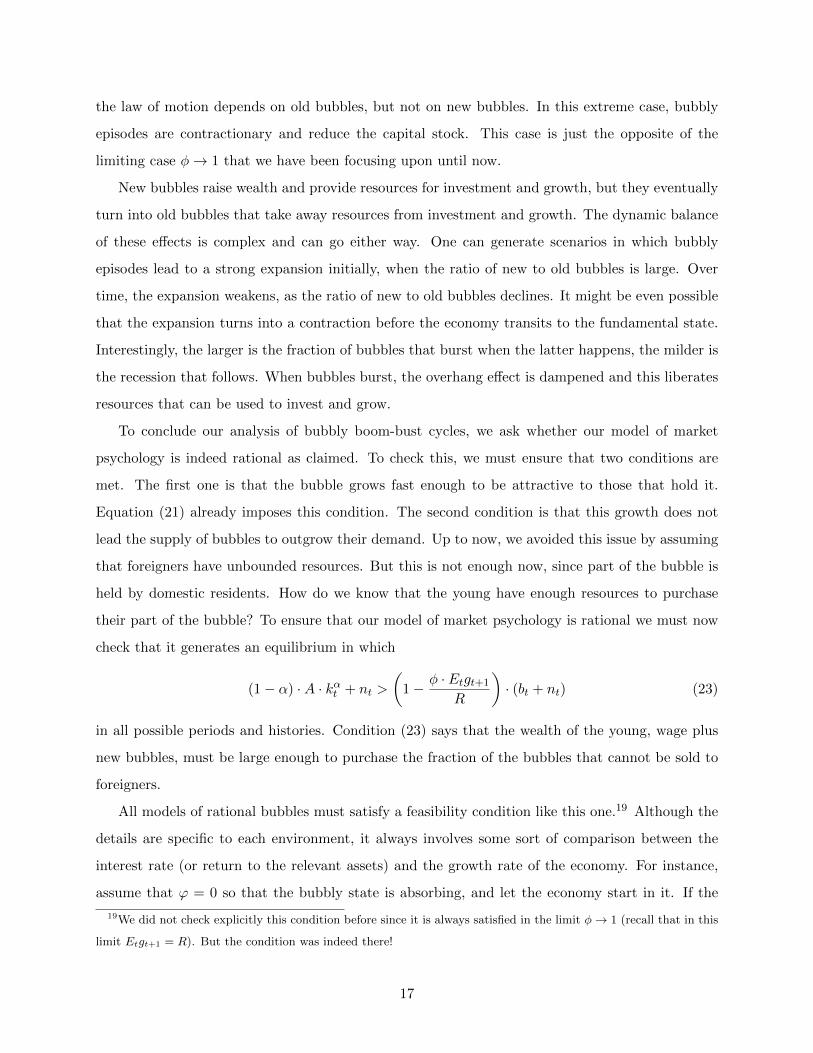
New bubbles raise wealth and provide resources for investment and growth, but they eventually

turn into old bubbles that take away resources from investment and growth. The dynamic balance

of these effects is complex and can go either way. One can generate scenarios in which bubbly

episodes lead to a strong expansion initially, when the ratio of new to old bubbles is large. Over

time, the expansion weakens, as the ratio of new to old bubbles declines. It might be even possible

that the expansion turns into a contraction before the economy transits to the fundamental state.

Interestingly, the larger is the fraction of bubbles that burst when the latter happens, the milder is

the recession that follows. When bubbles burst, the overhang effect is dampened and this liberates

resources that can be used to invest and grow.

To conclude our analysis of bubbly boom-bust cycles, we ask whether our model of market

psychology is indeed rational as claimed. To check this, we must ensure that two conditions are

met. The first one is that the bubble grows fast enough to be attractive to those that hold it.

Equation (21) already imposes this condition. The second condition is that this growth does not

lead the supply of bubbles to outgrow their demand. Up to now, we avoided this issue by assuming

that foreigners have unbounded resources. But this is not enough now, since part of the bubble is

held by domestic residents. How do we know that the young have enough resources to purchase

their part of the bubble? To ensure that our model of market psychology is rational we must now

check that it generates an equilibrium in which

(1− α) ·A · kαt + nt >

(1− φ · Etgt+1

R

)· (bt + nt) (23)

in all possible periods and histories. Condition (23) says that the wealth of the young, wage plus

new bubbles, must be large enough to purchase the fraction of the bubbles that cannot be sold to

foreigners.

All models of rational bubbles must satisfy a feasibility condition like this one.19 Although the

details are specific to each environment, it always involves some sort of comparison between the

interest rate (or return to the relevant assets) and the growth rate of the economy. For instance,

assume that ϕ = 0 so that the bubbly state is absorbing, and let the economy start in it. If the

19We did not check explicitly this condition before since it is always satisfied in the limit φ→ 1 (recall that in this

limit Etgt+1 = R). But the condition was indeed there!

17

borrowing limit is not binding, the bubble grows at the world interest rate, so that:

limt→∞

b =

R

γ −R· η if R < γ

∞ if R ≥ γ(24)

If R ≥ γ, the bubble grows without bound and eventually exceeds the wealth of the young. Standard

backward induction arguments rule this out, and this leads us to conclude that our assumed market

psychology is not rational in this case. If R < γ, the bubble converges to a finite value and Condition

(23) is satisfied if η is not too large.20 In this case, we conclude that our assumed market psychology

is rational. If the borrowing limit were not binding and/or the transition probability ϕ were positive,

the calculations would be more involved but the idea would be pretty much the same. The interest

rate must be low enough to ensure that the bubble does not outgrow the wealth of the young.

The bottom line of this discussion is that, for bubbly boom-bust cycles to happen, our lab

economy must be inserted into a world economy that is capable of supplying plenty of financing

(so that a large part of the bubble is exported) at low interest rates (so that the part of the bubble

that remains at home does not grow too fast). Is this a plausible description of the world economy?

Can such an environment explain the type of boom-bust episodes discussed in the introduction?

To answer these questions, we need to move beyond the borders of our lab economy and explore

the rest of the world.

2 The bubbly world economy

Many observers refer to the last 45 years as the era (or new era) of financial globalization.21 It

all started in the early 1970s in industrial countries, with the abandonment of the Bretton Woods

system and the removal of capital controls and many other restrictions to cross-border transactions.

The effects of this policy reversal were amplified by new trends in the 1980s. Industrial countries de-

regulated their financial markets, and new technologies facilitated the development of sophisticated

financial products. But the major impulse to financial globalization came in a second wave during

the early 1990s, when many emerging markets joined the world financial system. Up to then,

the private sectors in these developing economies had been prevented from participating in global

markets, which was a privilege retained by their sovereigns. The painful sovereign debt crisis of the

20If R ≤ φ · γ, Condition (23) is satisfied for any value of η. If φ · γ < R < γ, Condition (23) is satisfied if η is not

too large.21See, for instance Eichengreen and Bordo (2002), or Beck, Claessens and Schmukler (2013)

18

1980s uncovered the weakness of this model and led to its downfall. Capital controls were removed

and market-friendly policies were adopted throughout the emerging world.

The entry of emerging markets into the world financial system has coincided with profound

changes in the world economic environment. The first of these is cheap credit. Interest rates have

declined steadily since the early 1990s, reaching zero or even turning negative. Low interest rates

are a feature of systems with financial repression where funds are limited and rationed. But the

world financial system could not be farther away from such systems. If anything, financial markets

have incorporated large pools of savings from the emerging world, which move rapidly around the

globe in search of assets or stores of value.22 This is what Ben Bernanke famously described as

a global savings glut. As our lab economy showed us, low interest rates and plenty of financing

create the sort of environment that is conducive to bubbly boom-bust cycles. It is therefore not

surprising to find that financial integration with the emerging world has also been accompanied by

a marked increase in the frequency of credit booms and busts. More surprising, though, are the

so-called global imbalances, which refer to large capital flows from emerging economies with fast

productivity growth like China to advanced economies with slower productivity growth like the

United States. Most observers expected financial integration with emerging markets to be followed

by large capital flows in the opposite direction.

In this section, we use the theory of rational bubbles to explore the relationship between financial

globalization and bubbles. This relationship is complex and goes both ways, as we argue. Financial

globalization with emerging markets may well have created a bubble-friendly environment, but

bubbles have played a critical role shaping the effects of globalization as well. To show this, we

proceed again step by step, explaining first how to create bubbly environments, deriving then a

couple of important additional effects of old bubbles, and finally mixing all these ingredients to

develop a view of financial globalization with bubbles. We conclude the section by exploring the

implications for welfare and policy.

2.1 Creating bubbly environments

How do we create a bubbly environment? In the lab economy, it was just enough to assume that the

world interest rate, R, lies below the long-run growth rate, γ. Once we adopt a global perspective,

the world interest rate becomes an endogenous variable and it cannot be treated parametrically. A

bubbly environment is still a low interest rate environment. But to create one, we need to take a

22See, for instance, Caballero et al. (2008) and Coeurdacier et al. (2015).

19

detailed look at the determinants of the world interest rate.

Let us consider a world economy with many countries. All countries have the same population,

but they differ from the lab economy of the previous section in three respects. First, factor markets

are global and the wage and rental therefore depend on the world capital stock and not the country’s

capital stock. Thus, Equations (1)-(2) still apply, but now kt must be interpreted as the world

capital stock, and wt and rt as the common wage and rental.23 Second, only a fraction ε of each

country’s residents can manage and own capital. We refer to these individuals as entrepreneurs.

The rest cannot do so, and we refer to them as savers.24 Third, consumption goods are not

perishable and can be stored from one period to the next one. A literal way to think about storage

is as inventory accumulation. But there are other interpretations, as we shall show later. The rest

of our assumptions regarding preferences, technology, demography and domestic courts remain the

same as before.

As is customary by now, we must specify a market psychology to complete the model. We adopt

again the familiar market psychology of section 1.3. Recall that in this market psychology there is

no subsidy effect of bubbles, so that Equation (9) holds, and bubbles are fully pledgeable, so that

Equation (11) also applies. What kind of environments make such a market psychology rational?

What does the modeler have to do to create them?

The steady-state dynamics of the world capital stock are as follows:25

γ · kt+1 = min

{1

δ· [ε · (1− α) ·A · kαt + nt] , (1− α) ·A · kαt − bt

}(25)

The aggregate resource constraint of the economy says that the total wealth of the economy, which

consists of the wage, must be allocated to the three available assets: capital, bubbles, and storage.

23Since moving capital and labor physically is costly, the assumption of global factor markets can only be justified

if technologies allow factors of production located in different countries to embed their contributions to production in

specialized intermediate inputs. Trading these inputs would then lead to the equalization of factor prices. Technologies

have certainly evolved in this direction, and trade in intermediates has exploded in the last couple of decades. But

we are still far away from having factor markets that are truly global. We adopt this assumption because it helps

tremendously to provide clean and instructive derivations of the theoretical results we are after. But it is admittedly

unrealistic, and we shall remove it in section 2.3.24Since not all countries need to have the same proportion of savers, one could think of our lab economy as a

country without savers. But nothing of substance would really change from our analysis in section 1 if we added

savers to the lab economy. The only change would be that, when we referred to wealth, we would now refer to

“entrepreneurial” wealth. And when we referred to borrowing, we would now refer to “entrepreneurial” borrowing.25Here we are using the assumption that

α · γ1− α + 1− δ > 1. This condition implies that, in any steady state, the

return to investment is higher than the return to storage.

20

Equation (25) says that there are two regimes. In one regime, the interest rate equals the return

to storage, i.e., Rt+1 = 1, and the three assets are used in equilibrium. We refer to this case as the

“partial intermediation” regime. The borrowing limit is binding and some savings remain in the

hands of savers, who store them. Investment is limited or determined by entrepreneurial wealth.

In the second regime, the interest rate is higher than the return to storage:

Rt+1 = min

{γ · [(1− δ) · kt+1 + Etbt+1]

(1− ε) · (1− α) ·A · kαt, α ·A · kα−1t+1 + 1− δ

}(26)

and only capital and bubbles are held in equilibrium. We refer to this case as the “full intermedi-

ation” regime. The borrowing limit might be binding or not, but all savings end up in the hands

of entrepreneurs. If the borrowing limit is binding, the interest rate is determined by “cash-in-the-

market”, i.e. the ratio of entrepreneurial collateral to savings of the savers. If the borrowing limit

is not binding, the interest rate equals the return to investment.

The effects of bubbles depend on the regime. In the partial intermediation regime, the wealth

effect of new bubbles raises the capital stock at the expense of storage, with a constant interest

rate. Old bubbles have no effect on the capital stock. Thus, new and old bubbles have the same

effect as in the lab economy! But old bubbles are no longer held by foreigners with unbounded

resources. Instead, they are held by savers who reduce their holdings of stored goods. Interestingly,

this places a general-equilibrium limit to the effects of bubble creation: the complete elimination

of storage.

In the full intermediation regime, this limit has been reached and new bubbles no longer affect

capital accumulation. Interestingly, old bubbles have an overhang effect now. New and old bubbles

have the same effect as they did in the lab economy when they were not pledgeable, i.e. φ = 0.

But here we have assumed that they are pledgeable, i.e. φ = 1. What is going on? In the

economy of section 1.5, the overhang effect was a partial-equilibrium effect. Our assumption that

the bubble was not pledgeable forced entrepreneurs to hold part of it. The remaining part was

held by foreigners, and the latter had unbounded resources. Now, the overhang effect is a general-

equilibrium effect. Entrepreneurs need not hold any part of the bubble. But the rest of the world

no longer has unbounded resources. The larger is the bubble, the smaller are the resources that

are available for capital accumulation.

To create bubbly environments, note first that the equilibrium interest rate is (weakly) increasing

in the bubble. Calculate the steady-state interest rate in the absence of bubbles, i.e., in the history

21

in which the economy remains always in the fundamental state:

R∞ =

1 if ε < δ

min

{1− δ1− ε

,α · γ1− α

+ 1− δ}

if ε ≥ δ(27)

Since the interest rate is weakly increasing in the bubble, any equilibrium bubble must grow at

least at rate R∞. Thus, we need R∞ < γ for bubbles to be possible. Otherwise, any bubble would

eventually exceed the wealth of the economy. If R∞ < γ, a bubble can always exist and its size

will be limited by the need to keep the interest rate below the growth rate.26

The traditional literature on rational bubbles considers economies in which the borrowing limit

is not binding and R∞ equals the return to investment. This approach has been criticized on two

grounds however. Under these conditions, bubbles are only possible if additional investments are

dynamically inefficient and reduce steady state consumption. Abel et al. (1989) argued that this

condition was not met in the data, and even though Geerolf (2013) has recently challenged this view,

it is fair to say that most macroeconomists still believe that investment is dynamically efficient.

The second critique is that, if the borrowing limit is not binding, bubbles are contractionary and

should be associated with reductions in the capital stock and output. This seems to be contrary to

empirical evidence that shows that asset prices tend to be pro-cyclical. Mostly for these two reasons,

recent research on rational bubbles has focused instead on environments in which the borrowing

limit is binding and R∞ is lower than the return to investment. In this case, bubbles exist in

environments in which average investment is dynamically efficient and bubbles are expansionary.

We shall also follow this route here and, from now on, we focus exclusively on environments in

which the borrowing limit is binding.

We conclude this section with a comment on the concept of storage. A literal interpretation

of storage is inventory accumulation. But one could also interpret storage as low-quality capital,

as in section 1.4. In this case the return to “storage” would be ρ + 1 − δ instead of one. Thus, a

reduction in storage could also be interpreted as a reduction in inefficient investments. A simple

variation on the model shows that there is also a third possibility. Assume now that the young

attach a positive value to consumption during youth. In particular, young savers in generation t

maximize,

Ut = ct,t + β · Etct,t+1 (28)

26In some environments, bubbles lower the interest rate. In this case, they can exist even if R∞ > γ. Interestingly,

in this case small bubbles do not exist, but large enough bubbles that lower the interest below the growth rate do

exist. See Martin and Ventura (2012) for an example.

22

where β is the rate of time preference. Now, the return to “storage” would be β−1 instead of one.

Thus, a reduction in storage could also be interpreted as a reduction in early consumption. The

appropriate interpretation of “storage” depends on the context in which the theory is applied, and

the modeler has at least these three choices.

2.2 Are old bubbles always contractionary?

In the models we have developed so far new bubbles can only be expansionary while old bubbles

can only be contractionary. It seems to us that, under reasonable assumptions, the notion that new

bubbles are expansionary should be quite robust. But we know that the conclusion that old bubbles

are contractionary is not robust. To show this, we use now a popular market psychology according

to which no new bubbles are created, and either there is no bubble (the bubbleless equilibrium), or

the bubble has existed forever and it is stationary (the bubbly equilibrium). This market psychology

generates two possible steady-state situations with a constant bubble. A bubbleless steady state in

which the interest rate equals R∞, and a bubbly steady state in which the interest rate equals γ.27

Let us apply this market psychology first to the world economy of the previous section. The

law of motion of the capital stock is (recall that we are assuming from now on that the borrowing

limit is binding):

γ · kt+1 =Rt+1

Rt+1 + δ − 1· ε · (1− α) ·A · kαt . (29)

Thus, in any steady state we have that:

k =

[R

R+ δ − 1· ε · (1− α) ·A

γ

] 11−α

(30)

In the bubbleless equilibrium R = R∞, while in the bubbly equilibrium R = γ. Since the capital

stock declines with R, we just confirm our earlier finding that if bubbles exist, i.e. R∞ < γ; they

raise the interest rate and are therefore contractionary.

Let us now consider a simple modification of the model in which individuals live for three

periods: youth, middle age and old age. The young are endowed with 1 − ε units of labor, while

the middle-aged are endowed with ε units. Assume also that young individuals are savers, while

middle-aged individuals are entrepreneurs. Superficially, this model looks almost identical to the

one of the previous section. There are gains from intermediating resources between savers and

entrepreneurs, but financial frictions – and the wealth of entrepreneurs – limits the extent to which

27This type of modeling is quite restrictive, and we do not recommend it in applications. But it does simplify the

analysis dramatically, and this makes it convenient for theoretical explorations of specific mechanisms.

23

this can be done. But the life-cycle structure of this model introduces a crucial innovation: now,

the entrepreneurs of period t are the savers of period t−1, so that the wealth of the former depends

on the return to the savings of the latter.

The law of motion of the capital stock in this modified economy is given by:

γ · kt+1 =Rt+1

Rt+1 + δ − 1·[ε · (1− α) ·A · kαt +

Rtγ· (1− ε) · (1− α) ·A · kαt−1

]. (31)

The key novelty here is that entrepreneurial wealth has two components: wages plus the return to

savings. In any steady state, we now have that:

k =

[R

R+ δ − 1·(ε+

1− εγ·R)· (1− α) ·A

γ

] 11−α

(32)

It is not clear now whether the steady state capital stock is decreasing or increasing with R. On

the one hand, a high interest rate lowers the multiplier and reduces entrepreneurial leverage. This

is the familiar bubble overhang effect of old bubbles that lowers capital accumulation. On the other

hand, a high interest rate raises entrepreneurial wealth and this raises capital accumulation. This

is the liquidity effect of old bubbles since, by raising the interest rate, old bubbles make it cheaper

to carry funds across periods. If bubbles exist, i.e. if R∞ < γ, they still raise the interest rate.

But this need not be contractionary.28 To see this, consider the case in which δ = 1, so that the

financial multiplier equals one. The overhang effect vanishes, only the liquidity effect operates, and

old bubbles raise capital accumulation.

2.3 Financial globalization with bubbles

Let us now bring our focus back to financial globalization. To do this, we consider a world with

local factor markets and countries that differ in their level of financial development. In a subset of

countries j ∈ C, which we call Core, domestic courts can seize the revenues obtained through the

sale of firms so that their entrepreneurs face the familiar borrowing limit in Equation (3). In the

remaining set of countries j ∈ P , which we call Periphery, domestic courts are unable to seize any

income and their entrepreneurs cannot borrow. Let π be the share of the world population that

lives in Periphery countries. Throughout, we consider two possible market psychologies for each

country j. The first one is the fundamental one in which there are no bubbles nj,t = 0. The second

one is the bubbly market psychology we used in section 1.3 in which nj,t is given by Equation (9).

28In this modified model R∞ = max

{1,

1− δ1− ε ·

γ

γ + δ − 1

}< γ.

24

Consider an initial situation in which Core countries participate in a world credit market, but

Periphery countries do not (1970s and 1980s). The capital stocks of the different countries evolve

as follows

γ · kj,t+1 =Rt+1

Rt+1 + δ − 1·[ε · (1− α) ·A · kαj,t + nj,t

], for j ∈ C, (33)

γ · kj,t+1 = ε · (1− α) ·A · kαj,t + nj,t, for j ∈ P . (34)

The main difference between capital accumulation in Core and Periphery countries is the size of

the financial multiplier. This multiplier is above one in Core countries, since their entrepreneurs

are subject to the borrowing limit in Equation (3). The financial multiplier is one in Periphery

countries, since their entrepreneurs cannot borrow. The interest rate in Core countries is given by:

Rt+1 = max

γ ·∑j∈C

[(1− δ) · kj,t+1 + Etbj,t+1]

(1− ε) · (1− α) ·A ·∑j∈C

kαj,t, 1

. (35)

If their combined entrepreneurial collateral is large enough relative to the wealth of their savers,

the interest rate in Core countries is determined by “cash-in-the-market” and storage is not used

in equilibrium. Otherwise, the interest rate equals one and storage is used in equilibrium. In

Periphery countries, the interest rate equals one so that savers are indifferent between storage and

credit. However, this interest rate is only notional since the equilibrium amount of credit is zero.

Entrepreneurs would like to borrow at this rate, but they have no collateral to offer. Periphery

savers are forced to use storage.

Let us assume that:

γ <1− δ1− ε

< ε−1 · α · γ1− α

+ 1− δ. (36)

In Core countries, bubbles are fully pledgeable and their expected growth must equal the world

interest rate. But the first inequality in assumption (36) says that this interest rate is above the

growth rate. In Periphery countries, bubbles are not pledgeable and their expected growth in

equilibrium must equal the return to investment. But the second inequality in assumption (36)

says that this return to investment is above the growth rate. Thus, bubbles are not possible in

any country. The only feasible market psychology is the fundamental one and the Core-Periphery

world exhibits quiet dynamics. There are no shocks and all countries monotonically converge to

their respective steady states. Given that countries differ only in their level of financial development,

there is full convergence within regions but not across regions. Core countries converge to a steady

state with a higher capital stock and a higher interest rate than Periphery countries.

25

Let us consider now what happens if Periphery countries join the world credit market (1990s-

today). The world interest rate, which now applies to all countries, becomes:

Rt+1 = max

γ ·∑j∈C

[(1− δ) · kj,t+1 + Etbj,t+1]

(1− ε) · (1− α) ·A ·∑

j∈C∪Pkαj,t

, 1

. (37)

The entry of Periphery countries into the world financial market does not raise entrepreneurial

collateral, because Periphery entrepreneurs are still unable to borrow due to the inefficiency of

their domestic courts. But Periphery savers can now lend to Core entrepreneurs, and this raises the

wealth of savers in the market. Thus, the world interest rate drops and capital flows from Periphery

to Core. These capital flows raise world efficiency because they convert Periphery storage into Core

capital.

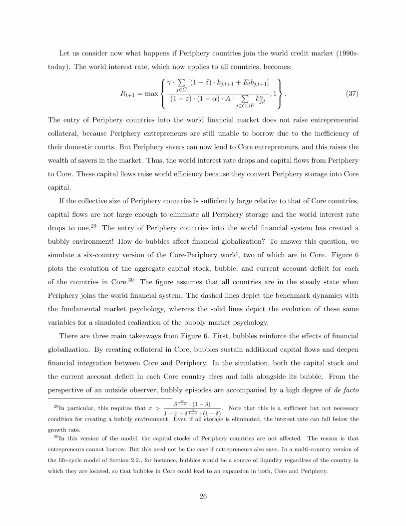
If the collective size of Periphery countries is sufficiently large relative to that of Core countries,

capital flows are not large enough to eliminate all Periphery storage and the world interest rate

drops to one.29 The entry of Periphery countries into the world financial system has created a

bubbly environment! How do bubbles affect financial globalization? To answer this question, we

simulate a six-country version of the Core-Periphery world, two of which are in Core. Figure 6

plots the evolution of the aggregate capital stock, bubble, and current account deficit for each

of the countries in Core.30 The figure assumes that all countries are in the steady state when

Periphery joins the world financial system. The dashed lines depict the benchmark dynamics with

the fundamental market psychology, whereas the solid lines depict the evolution of these same

variables for a simulated realization of the bubbly market psychology.

There are three main takeaways from Figure 6. First, bubbles reinforce the effects of financial

globalization. By creating collateral in Core, bubbles sustain additional capital flows and deepen

financial integration between Core and Periphery. In the simulation, both the capital stock and

the current account deficit in each Core country rises and falls alongside its bubble. From the

perspective of an outside observer, bubbly episodes are accompanied by a high degree of de facto

29In particular, this requires that π >δ

α1−α · (1− δ)

1− ε+ δα

1−α · (1− δ). Note that this is a sufficient but not necessary

condition for creating a bubbly environment. Even if all storage is eliminated, the interest rate can fall below the

growth rate.30In this version of the model, the capital stocks of Periphery countries are not affected. The reason is that

entrepreneurs cannot borrow. But this need not be the case if entrepreneurs also save. In a multi-country version of

the life-cycle model of Section 2.2., for instance, bubbles would be a source of liquidity regardless of the country in

which they are located, so that bubbles in Core could lead to an expansion in both, Core and Periphery.

26

financial integration, whereas reversals to the fundamental state are accompanied by retrenchment.

This leads to the second point, which is that the capital flows sustained by bubbles are volatile.

Indeed, as the figure shows, Core countries experience surges in inflows and sudden stops driven

solely by market psychology. Third, because they are country-specific, bubbles lead to dispersion

within Core. Although both Core countries are fundamentally identical to one another, market

psychology can favor any one of them over the other. The general insight here is that the global

allocation of savings will be determined both by bubbles and by productivity and, in principle,

there is no reason for both forces to coincide.

2.4 Managing bubbles

Up to now, we have focused exclusively on the positive aspects of bubbles, namely when they can

exist and how they affect macroeconomic dynamics. We have shown the reader how the theory

of rational bubbles can help us interpret the boom-bust episodes of recent years. We now turn to

some normative issues and explore both the desirability of bubbles and the role, if any, of policy in

managing them. Both questions have been the object of a lively, if often unstructured, debate in

the academic and policy communities. But the theory of rational bubbles has much to offer to this

debate.

In the bubbly economy, market psychology is an essential component of equilibrium. This

raises two central questions. Which is the most desirable market psychology? Can the policy

maker implement it? Much has been written about these questions, and a thorough treatment of

them would require more space than we have at our disposal. We therefore address them within

the context of a particular example, the Core-Periphery world of the previous section. Although

the setting is specific, the insights that it delivers are easily generalizable to other environments.

2.4.1 What should governments do?

We return to the Core-Periphery world and assume that there is a global planner with the ability

to coordinate the market on its preferred psychology. Which one would she select? Answering this

question requires defining the objective function of the planner. This is not trivial because bubbles

entail a complex web of intra- and inter-generational transfers. One common approach, which we

adopt here, is to assume that the planner’s goal is to maximize some measure of welfare in the

steady state. Since the only source of uncertainty in this world is market psychology itself, the

planner selects a “deterministic” market psychology with a constant rate of bubble creation , i.e.,

27

nj,t = ηj , and no shocks to the return of old bubbles, i.e., gj,t+1 = Rt+1, for all t and j ∈ C. Note

that we need only specify the market psychology for Core, as we know that in Periphery the only

admissible psychology is nj,t = bj,t = 0, for all t and j ∈ P .

All market psychologies of this type yield a deterministic steady state, which is characterized

by the following set of equations:

kj =g

g + δ − 1·[ε ·A · (1− α) · kαj + ηj

]for j ∈ C, (38)

kj =

[ε ·A · (1− α)

γ

] 11−α

for j ∈ P , (39)

g = max

γ ·∑j∈C

[(1− δ) · kj + bj ]

(1− ε) · (1− α) ·A ·∑

j∈C∪Pkαj, 1

. (40)

where g denotes the world interest rate, which must equal the growth rate of bubbles in all countries.

Equation (38) implicitly defines the steady-state capital stock in Core countries solely as a function

of g and ηj . Equation (39) instead shows that, because its entrepreneurs are cut-off from the

credit market, the capital stock in Periphery is independent of bubbles and the world interest rate.

Equation (40), in turn, characterizes the world interest rate. Finally, note that there are two market

psychologies under which bj > 0: if g = γ, it must be that ηj = 0, or; if g < γ, it must be that

ηj > 0 and bj = ηj · g · (γ − g)−1.31

Which psychology would a global planner choose? To answer this question, let us first cha-

racterize the set of Pareto-optimal allocations. This may seem like a complicated task, given that

this world is populated by savers and entrepreneurs in many different countries. But it is actually

quite simple.32 An allocation can only be Pareto-optimal if storage is not used. The intuition is

simple: if storage is being used, it is always possible to increase bubble creation – and thus invest-

ment – in some country without reducing investment (and therefore welfare) anywhere else. Once

31Indeed, by evaluating Equation (8) in steady state and setting nj,t = ηj for all t, we obtain,

γ · bj = g · (bj + ηj) , for j ∈ C,

so that bj > 0 only if γ = g and ηj = 0, or if γ > g in which case,

bj =g

γ − g · ηj .

32In Core, the welfare of entrepreneurs equals only the rental income of capital because undepreciated capital has

been fully pledged to creditors. In Periphery, instead, the welfare of entrepreneurs equals the entire capital income.

The steady-state welfare of savers, in turn, equals their labor income times the market interest rate.

28

storage is completely eliminated, any additional increase in bubble creation comes at the expense

of investment somewhere else and cannot be Pareto-improving.

Indeed, there is a continuum of Pareto-optimal allocations in the Core-Periphery world, each

of them sustained by a different market psychology. Although the use of storage is eliminated in

all of them, these allocations differ in their bubbles, their capital stocks, and their interest rates,

which can lie anywhere between 1 and γ. Whether one market psychology is preferred over another

depends on the relative weights that the global planner assigns to the different type of individuals.

If the planner favors entrepreneurs, she will prefer allocations with the lowest interest rate to

maximize investment. If instead the planner favors savers, she may prefer allocations with higher

interest rates even if this comes at the expense of investment.

This discussion illustrates some key normative implications of the theory of rational bubbles.

Perhaps the main one is that, far from the widespread notion that bubbles are undesirable, the

theory suggests that they can be Pareto-improving.33 Naturally, different bubbles have different

effects on global output and its distribution.34 But characterizing the set of optimal bubbles is

only the first step towards a proper analysis of policy. The other is thinking about implementation,

which raises further questions of its own. First, the world is not run by a global planner but rather

by a collection of individual governments. It is natural to expect each government to favor bubble

creation in its own economy even if this comes at the expense of investment elsewhere in the world.

As in other areas of international economics, this creates a need for policy coordination on which

we shall not elaborate here. We turn instead to a second crucial point: once governments have

decided on their preferred market psychology, what can they do to induce it?

2.4.2 What can governments do?

This section considers the problem of governments that, having settled on a preferred market

psychology, want to implement the corresponding allocation. One possible approach is to assume

that governments can choose this psychology directly, for instance, by forcing individuals to act

in a certain way and punishing those that deviate. This is not very interesting, however. An

33This need not be the case, of course, as bubbles may also entail costs. They may redirect investment towards

unproductive uses, as we have seen, they may be too volatile, or they may become too large thereby leading to

inefficiently severe crises when they burst (see, for instance, Caballero and Krishnamurthy 2006).34These effects of bubbles, moreover, are model-specific. In the Core-Periphery world, for instance, it is the wealth

effect of bubble creation that enables entrepreneurs to expand their investment. In the life-cycle model of Section

2.2., instead, the liquidity effect of old bubbles can do the trick.

29

alternative approach, which we have developed over various papers and follow here, is to endow

governments with specific policy tools and study how these tools can be used to re-create the

transfers implemented by the preferred bubble, thereby implementing the desired allocation.35

Since bubbles implement these transfers through the credit market, it is reasonable to begin by

looking at credit market interventions.

Let us assume that governments want to implement the Pareto-optimal allocation associated

with market psychology {ηj}j∈C . To do so, we assume that governments in Core are able to

subsidize and/or tax their entrepreneurs. In particular, we assume that the government of country

j ∈ C promises to give its entrepreneurs of generation t a gross transfer of sj,t+1 units of the

consumption good during old age. These transfers can be negative and/or contingent on the state

of the economy, and we assume that they can be pledged by entrepreneurs to outside creditors.

We do not allow for cross-country subsidies, though. Thus, positive transfers in country j ∈ C are

financed through a tax on the country’s young entrepreneurs; negative transfers, in turn, generate

a revenue that is distributed among young entrepreneurs.

These interventions can be thought of as credit management policies. Given policies {sj,t}j∈Cfor all t, we can define:

nsj,t =γ · Etsj,t+1

g− sj,t. (41)

Thus, nsj,t represents the net transfers to young entrepreneurs in country j, i.e., the difference

between the present value of subsidies that they will obtain in old age and the taxes paid in young

age. This difference can be positive or negative. The key observation is that there are now three

sources of entrepreneurial wealth: wages, new bubbles, and net transfers, i.e., entrepreneurial wealth

equals wj,t + nj,t + nsj,t. Moreover, there are now three sources of collateral: undepreciated capital,

bubbles, and gross transfers, i.e., collateral equals (1− δ) · kj,t+1 + Et {bj,t+1 + sj,t+1}.

As this discussion makes it clear, these interventions replicate the effects of bubbles. For in-

stance, to implement the desired allocation, governments simply need to set sj,t = bj − bj,t, which

implies that nsj,t = ηj − nj,t for any market psychology {nj,t}j∈C . That is, governments can repli-

cate any allocation by appropriately designing state-contingent policies! In our case, this requires

“leaning against market psychology”. In countries and times where the bubble is low relative to

the desired benchmark, the policy requires the corresponding government to subsidize credit. In

countries and times where the bubble is high relative to the desired benchmark, the policy requires

the corresponding government to tax credit.

35See, for instance, Martin and Ventura (2015, 2016).

30

A salient feature of these policies is that they are expectationally robust, in the sense that they

implement the desired allocation regardless of market psychology. That is, they do not target asset

prices, but instead insulate the economy from their fluctuations. Note that these policies achieve

their objectives even if their adoption changes market psychology.

Bubbles create a web of inter and intra generational transfers. The key insight of this section is

that, if governments have the necessary tools to replicate these transfers, they can always replicate

the desired bubble. We have focused here on the case of taxes and subsidies on credit, but nothing

changes if we allow governments to finance these policies through debt. Moreover, depending on

the setup, these interventions can also be interpreted as capital controls or bailouts.

What if governments do not have this full set of tools at their disposal? They may, for instance,

have only a limited ability to tax and/or subsidize entrepreneurs. Or, as in some monetary models,

they may be able to influence the real interest rate, which in turn determines the equilibrium growth

rate of old bubbles. Although such limitations certainly curtail governments’ ability to replicate

a desired bubble, they do not change the general nature of the problem. At times, the observed

bubble is too small relative to the desired one and policy should try to raise its size; at other times,

the observed bubble is too large relative to the desired one and policy should try to reduce its size.

3 A guide to the literature

In the previous sections, we have used simple models and examples to convey the main positive and

normative insights of the theory of rational bubbles for macroeconomics. We now provide a brief

guide to the literature that has developed these insights and built on them to generate additional

results.

3.1 The traditional view of bubbles

The seminal papers in the theory of rational bubbles are Samuelson (1958) and Tirole (1985).

Samuelson showed how, in an endowment economy with overlapping-generations, rational bubbles

could offer a remedy to the problem of dynamic inefficiency. Tirole extended these insights to the

classic Diamond (1965) model of capital accumulation, providing the first full treatment of bubbles

in a production economy. We describe below his results.

In the absence of frictions, the interest rate in the Diamond (1965) model equals the marginal

return to investment, i.e., the return to capital accumulation. It is well-known that the equilibrium

31

in this model can be dynamically inefficient, which happens whenever the steady-state interest

rate lies below the growth rate of the economy. These are situations in which the capital stock is

excessive and its return is too low. Tirole (1985) showed that, in such situations, there exists an

alternative bubbly steady state in which agents are willing to hold rational bubbles. This steady

state has two key features relative to the standard fundamental one. First, both the capital stock

and output are lower, because bubbles divert resources away from capital accumulation. This is

nothing but the overhang effect of old bubbles that we have discussed so extensively. Second,

welfare is higher, because the capital stock eliminated by the bubble is inefficient to begin with.

Both results correspond exactly to our analysis of the world economy of section 2.1, for the case in

which the borrowing limit is not binding.

These first findings were derived in highly stylized models and it was not obvious how robust they

were to some natural generalizations of the environment. One such generalization is the inclusion

of non-reproducible factors of production such as land, which provide rents to their owners. In

equilibrium, the price of these factors must equal the discounted value of the stream of rents that

they are expected to generate in the future. This is problematic, because dynamic inefficiency –

which generates the low interest rates necessary for the existence of bubbles – may imply infeasibly

high prices of non-reproducible factors. Tirole (1985) partially explored this connection and showed

that sometimes, in the presence of rents, the unique market psychology must feature a bubble! Rhee

(1991) focused specifically on land, and showed that its presence is not incompatible with dynamic

inefficiency insofar as the land share of output vanishes asymptotically.

Another unappealing feature of this early work is that it focused on deterministic bubbles, which

display a very predictable behavior and never burst. The fact that real-world bubbles are anything

but predictable prompted the study of stochastic bubbles like the ones we have used throughout this

guide. Blanchard (1979) and Blanchard and Watson (1982) used partial-equilibrium asset-pricing

models to show that such bubbles can be consistent with rational expectations. They also argued

that stochastic bubbles could display a wide range of behavior, and studied conditions under which

their presence could be verified econometrically. Weil (1987) studied the existence of stochastic

bubbles in general equilibrium, extending Tirole (1985) to the case of bubbles that have a constant,

exogenous, probability of collapsing.

This theory of rational bubbles provided an elegant and powerful way to think about real-world

bubbles, suggesting that it would be widely used by macroeconomists. But this did not happen.

A first drawback of the theory is its prediction that bubbles can only arise under low interest

32

rates, which – in the basic models discussed above – is equivalent to dynamic inefficiency. As we

anticipated in section 2.1, the empirical validity of the latter was questioned in an influential paper

by Abel et al. (1989). Although their findings have been recently questioned by Geerolf (2013),

the predominant view has been for many years that real economies are dynamically efficient. This

appeared to limit the relevance of the theory of rational bubbles, but only if one sticks to the

frictionless models in which the theory was first developed. In the presence of frictions, in fact,

the interest rate need not accurately reflect the return to capital and bubbles may exist even if the

economy is efficient.

One set of papers made this point in the context of endogenous growth. Saint-Paul (1992),

Grossman and Yanagawa (1993), and King and Ferguson (1993), for instance, extended the analysis

of Tirole (1985) to economies with endogenous growth due to externalities in capital accumulation.

The key insight of these papers is that, in the presence of such externalities, the market interest

rate underestimates the true return to investment. Thus, the interest rate can be low enough

for bubbles to exist even if the economy is dynamically efficient. In these models, bubbles reduce

capital accumulation exactly as in Tirole (1985). But their welfare implications are different because

these economies accumulate too little, as opposed to too much, capital to begin with. By reducing

capital accumulation, bubbles slow down the long-term growth rate of the economy so that there

always exists a future generation that is harmed. Note that these insights are closely related to

our discussion of the Dutch disease in section 1.4., and they would also arise in our example in the

presence of externalities.

Another set of papers showed that bubbles could arise in dynamically efficient economies if

there are financial frictions. Woodford (1990), Kocherlakota (1992), Azariadis and Smith (1993),

and Woodford and Santos (1997), for instance, showed how frictions such as borrowing constraints

and adverse selection could depress equilibrium interest rates and create bubbly environments. The

role of various financial frictions in creating this type of environments has since then been analyzed

in the literature, from the lack of insurance markets (e.g. Aoki et al. (2014)) to borrowing limits

like the ones we have explored here (e.g. Hirano and Yanagawa (2016)).

3.2 A new view of bubbles

Even if one accepts that the existence of bubbles does not require dynamic inefficiency, there is a

second implication of the basic models that seemed unpalatable; namely, bubbles crowd out capital

accumulation and reduce output. This prediction seemed particularly troubling in the aftermath of

33

the dot-com boom and bust of the late 1990s, during which the performance of the United States

economy closely tracked the growth and subsequent collapse of the stock market. If there was ever

a boom-bust episode where the theory of rational bubbles should apply, this was it. And yet, it

highlighted the theory’s limitations.

To address this issue, Olivier (2000) used an endogenous growth model to show that the effects

of bubbles depend on the asset on which they appear. Bubbles on equity, in particular, can raise

the market value of firms thereby enhancing firm creation, investment, and growth. Bubbles on

unproductive assets, in turn, have the typical crowding-out effect and reduce growth. The key

insight of the model, in fact, is that bubbles on equity have similar effects to subsidies on R&D.

This is closely related to the subsidy effect of section 1.4., with the difference that Olivier (2000)

focuses on the case in which the bubble subsidizes productive investment.

But most of the recent literature on rational bubbles has focused instead on models with fi-

nancial frictions. This has been partly due to the widespread introduction of financial accelerator

mechanisms, like those in Bernanke and Gertler (1989) and Kiyotaki and Moore (1997), into ma-

croeconomic models. Financial frictions not only relax the conditions for the existence of bubbles,

as we have already mentioned, but they also enable bubbles to expand the capital stock and output.

Different strands of literature emphasize different mechanisms for this expansionary effect, most of

which have already been discussed throughout this guide. The common theme that underlies all

of them is that bubbles enable the transfer of resources, from agents who do not want to invest to

those that do.

A first strand of the literature stresses the wealth effect of bubble creation, which we first in-

troduced in Martin and Ventura (2012) and has since then been explored in a series of papers. In

these models, newly created bubbles reallocate resources because they are sold by productive to

unproductive agents, either directly or indirectly through the credit market. This wealth effect of

bubble creation has been a recurrent theme throughout sections 1 and 2, and we shall not dwell

on it here. It suffices to say that all the main insights derived in the context of our stylized exam-

ples survive in richer environments, with more general preferences and alternative credit market

specifications (see Martin and Ventura 2011, 2015 and 2016).

A second strand of literature stresses the role of bubbles as providers of liquidity, as in the

model of section 2.2. In these models, bubbles enable agents to transfer resources over time, from

periods in which they are unproductive to periods in which they are productive. Thus, rational

agents are willing to hold bubbles because they expect to sell them or borrow against them in the

34

future, when the time comes to invest. Some examples of this line of research include Caballero

and Krishnamurthy (2006), Kocherlakota (2009), Farhi and Tirole (2012), Miao and Wang (2017)

and Guerron-Quintana et al. (2017).

Finally, a third strand of literature highlights the general equilibrium effects of bubbles, which

can induce price changes that enable the transfer of production factors from unproductive to pro-

ductive agents. Ventura (2012) and Ventura and Voth (2015), for instance, study environments in

which unproductive and productive agents compete for existing factors of production like capital

and labor. When unproductive agents purchase bubbles, they reduce their production and thus

their demand for capital and/or labor. The consequent fall in the price of these factors enable

productive but constrained agents to expand their production, thereby leading to a boom.

3.3 Macroeconomic applications

Building on these insights, there has been an explosion of research in recent years trying to explain

a wide array of macroeconomic phenomena.

Let us start with financial markets. There is mounting evidence of a link between asset bubbles,

credit booms and busts, and financial crises (e.g. Schularik and Taylor (2012), Jorda et al. (2015)).

Martin and Ventura (2016) and Miao and Wang (2017) explore this connection in general equili-

brium models of credit and bubbles, in many ways similar to the world economy of section 2.1. In

these models, the bursting of a bubble pushes the economy into a recession but it does not lead

to defaults or unemployment because credit contracts are state-contingent and prices are flexible.

In related settings, Ikeda and Phan (2016) and Bengui and Phan (2016) introduce non-contingent

contracts to generate defaults, while Miao and Wang (2016) and Hanson and Phan (2017) introduce

nominal rigidities to generate unemployment.

Delving deeper into financial markets, various papers have explicitly introduced financial inter-

mediaries to analyze how their presence shapes the effects of bubbly booms and busts. Aoki and

Nikolov (2015), Miao and Wang (2015), Martin and Ventura (2016 online appendix), and Freixas

and Perez-Reyna (2016) are some examples in this regard. In general, these models are similar

to the examples explored throughout this guide, with the difference that both entrepreneurs and

financial intermediaries are subject to borrowing limits. Bubbles can relax or tighten these limits

for financial intermediaries through the same mechanisms outlined above. The key insight is that

it is not just the size of the bubble, but also its location – i.e., whether it is created and/or held by

financial intermediaries or entrepreneurs – that matters for economic activity.

35

The location of a bubble is also important in determining the allocation of resources across firms

and sectors. Queiros (2017a) provides empirical evidence in this regard. Miao and Wang (2014),

Basco (2016) and Tripathy (2017) develop models to study the role of bubbles in determining the

cross-sector allocation of resources. Much in the spirit of the subsidy effect discussed in section 1.4,

these papers identify conditions under which bubbles can reduce efficiency (and potentially growth)

by reallocating resources towards less productive uses. One specific sector that has received much

attention is housing, both because of its size and because it exhibits large fluctuations. Arce and

Lopez-Salido (2011), Basco (2014), Zhao (2015), and Huber (2016) develop models of rational

bubbles to study the macroeconomic implications of fluctuations in housing. Finally, for all this

sector-level research, there has been almost no work on the firm-level implications of bubbles. This

is somewhat surprising given the growing interest of macroeconomists on firm dynamics. Two

exceptions are Tang (2017) and Queiros (2017b), who study models of heterogeneous firms with

entry and exit and explore the effects of bubbles on competition, on average productivity, and on

its dispersion across firms.

On the international sphere, bubbles affect the allocation of resources across countries, as we

illustrated through the Core-Periphery world. The role of bubbles in shaping the size, direction,

and volatility of capital flows has been explored in a number of papers. Kraay and Ventura (2007)

and Ikeda and Phan (2015) use models of rational bubbles to account for global imbalances between

the United States and the developing world. Basco (2014) and Rondina (2017) are closest to the

Core-Periphery example in section 2.3, as they provide formal models in which, due to asymme-

tric financial development, financial globalization itself creates a bubbly environment. In Martin

and Ventura (2015), we construct a multi-country model and explore the positive and normative

implications of bubbles for capital flows and for the global allocation of resources.

Finally, there is a large literature on the ability (or not) of macroeconomic policy to manage

bubbles and their effects. Here, the desirability and effectiveness of policy depends on the tools at

the authority’s disposal. In Martin and Ventura (2015, 2016), we provide a formal analysis of the

policy results illustrated in section 2.4, which assume that the government has the necessary tools

to reproduce the transfers induced by bubbles. In Martin and Ventura (2011, 2016), we also explore

whether a government with limited ability to tax can nonetheless manage bubbles by issuing public

debt. Arce and Lopez Salido (2011) study policy interventions meant to eliminate bubbles on the

“wrong” assets, which generate distortions, and foster them on the “right” assets. Other papers

have focused not on the ability of policy to replicate the desired bubble, but rather on its role in

36

preventing crises or mitigating their effects. These interventions can be both ex ante in the form

of macroprudential regulation (e.g. Caballero and Krishnamurthy 2006), or ex post in the form of

bailouts (e.g. Hirano et al. 2015).

Most of this literature on policy has a fiscal flavor to it, focusing almost exclusively on the

role that taxes and subsidies can play in managing bubbles. The role of monetary policy has been

much less explored, although it has featured prominently in the academic and policy debate for a

long time (e.g. Bernanke and Gertler 2001). This is now changing. Gali (2014) and Barlevy et al.

(2017) study how a monetary authority can, by controlling the interest rate, affect the evolution

of bubbles. Asriyan et al. (2016) construct a model of money, credit and bubbles and show that

market psychology can itself be a source of nominal rigidity if expectations are set in nominal

terms. They also explore the general equilibrium effects of bubbles, and of monetary policy, both

outside and inside of the liquidity trap. More recently, Gali (2017), Ikeda (2017) and Dong et al.

(2017) explore the interaction of monetary policy and bubbles in models with nominal rigidities

and long-lived agents, which renders these models more suitable for quantitative analysis.

The key takeaway from these papers is not that policy should eliminate bubbles, as is commonly

argued in informal discussions. Rather, policy should “lean against market psychology”, making

the bubble larger when it is too small and reducing it when it is too large.

This brings us to our last point on this tour of the literature. Most of the papers surveyed

here use OLG structures with short lifespans, which are extremely useful to explore the theoretical

mechanisms at hand. These models are hard to solve once individuals are long-lived, however,

because they give rise to a large degree of inter-generational heterogeneity. This is one of the

reasons for which macroeconomics has adopted models with infinitely-lived agents for quantitative

work. These models, however, are known to be inconsistent with rational bubbles. So how do we

construct macroeconomic models of rational bubbles for quantitative analysis?

There are currently two approaches being explored in the literature. The first is to develop

OLG models with perpetual youth as in Yaari (1965) and Blanchard (1985), in which agents face

a certain probability of death: these models have the advantage of preserving the OLG structure,

and thus all of the basic results discussed above, while maintaining tractability for quantitative

analysis. This is the approach recently adopted by Gali (2017). The second approach, used by

Kocherlakota (2009) and Miao and Wang (2017) among others, is based once again on financial

frictions. In a nutshell, it consists of assuming that some assets have a special status as collateral.

From the perspective of potentially constrained agents, bubbles on these assets have the additional

37

benefit – over and above their growth rate – of relaxing the borrowing limit. Hence, bubbles need

not grow at the rate of interest to be attractive and may exist in infinite horizon models. Although

an in-depth discussion of this approach is beyond the scope of this guide, we refer the interested

reader to Miao (2014) for a survey.

4 Where do we go from here?

This paper has provided a user’s guide to the theory of rational bubbles for macroeconomists. It

has sought to introduce macroeconomists to the main positive and normative aspects of the theory,

and to illustrate its usefulness in accounting for important macroeconomic phenomena. We would

like to conclude by pointing out the two main challenges that we see as the literature moves forward.

The first challenge is empirical. To assess the macroeconomic effects of bubbles, we need to

measure them. This is difficult, because the fundamental value of an asset is not observable.

Thus, any attempt to compare an asset’s market and fundamental values is only as reliable as the

underlying model that is used to assess fundamentals. This problem lies at the heart of the large

discrepancy of findings in the empirical literature on bubbles.36 Most of this literature, moreover,

tests for the existence of bubbles in a particular asset or asset class. From a macroeconomic

standpoint, it seems more relevant to measure the aggregate bubble, i.e. the bubble component of

the economy’s entire stock of assets.

Measuring this aggregate bubble may seem like wishful thinking. But macroeconomists have

experience measuring unobservables, most notably the aggregate productivity of an economy. More

than half a century ago, Solow taught the profession how to use aggregate input and output data

to derive a model-based measure of aggregate TFP. In much the same vein, macroeconomists could

use data on asset prices and aggregate capital income from the national accounts to derive a model-

based measure of the economy’s aggregate bubble, or an aggregate “bubble residual”. In Carvalho

et al. (2012), we took a first step in this direction and used national accounts to estimate the

fundamental value of household net worth in the United States between 1950 and 2010. We found

large discrepancies between this estimated value and the actual net worth as reported in the Federal

Reserve’s flow of funds data, especially during recent decades. But our exercise merely scratched

the surface, and there is much to be done along this front.

The second challenge is both empirical and conceptual. One of the running themes of this guide

36Two excellent examples are Froot and Obstfeld (1991) and LeRoy (2004). See Gurkaynak (2008) for a survey.

38

is that, in standard macroeconomic models, multiplicity may be more prevalent than we typically

care to admit. Once we accept that there may be many market psychologies that are consistent with

rationality, how do we chose among them? Should we choose the market psychology that, within a

set of constraints, best fits the data? This is the approach recently used by Guerron-Quintana et

al. (2017), who develop a macroeconomic model of bubbles and use it to estimate the persistence

and volatility of productivity and psychology shocks on post-war US data (incidentally, the data is

strongly consistent with the presence of bubbles). An alternative and complementary strategy is

to appeal to theory and develop new refinement techniques that can be used to reduce the set of

admissible market psychologies.

These challenges are far from minor, and they raise difficult questions going forward. But they

also point to an exciting path ahead, one that must be tread on if the theory of bubbles is to

become an integral part of the macroeconomist’s toolkit.

39

5 Figures

1983 1988 1993 19984.5

5.0

5.5

6.0

6.5

7.0Japan private net worth/GDP

1983 1988 1993 1998

1.5

2.0

2.5

3.0

3.5

4.0

Japan CA as % of GDP

1983 1988 1993 1998

05

0

5

10

So−rc s: / a%th data: /or%d / a%th and incom databas , other data: JST (2017)

Japan growth rates (annual)

RGDP Real Consumption pc Real Investment

Figure 1: Bubbly episode in Japan.

40

1993 1998 2003 2008 20133.5

4.0

4.5

5.0

USA private net worth/GDP

1993 1998 2003 2008 201306

05

04

03

02

01USA CA as % of GDP

1993 1998 2003 2008 201302

0

2

4

So−rc s: / a%th data: /or%d / a%th and incom databas , other data: JST (2017)

USA growth rates (annual)

RGDP Real Consumption pc Real Capital

Figure 2: Dot-com and housing boom in USA.

41

1993 1998 2003 2008 20134.5

5.5

6.5

7.5

8.5Spain private net worth/GDP

1993 1998 2003 2008 2013010.0

07.5

05.0

02.5

0.0

Spain CA as % of GDP

1993 1998 2003 2008 2013020

010

0

10

So−rc s: / a%th data: /or%d / a%th and incom databas , other data: JST (2017)

Spain growth rates (annual)

RGDP Real Consumption pc Real Investment

Figure 3: Housing boom in Spain.

42

2002 2004 2006 2008 2010 20122.5

3.0

3.5

4.0Ireland private net worth/GDP

2002 2004 2006 2008 2010 2012

−6

−4

−2

0

2Ireland CA as % of GDP

2002 2004 2006 2008 2010 2012−20

−10

0

10

20

Sources: wealth: Central Bank of Ireland, other data: OECD

Ireland growth rates (annual)

RGDP Real Consumption pc Real Investment

Figure 4: Housing boom in Ireland.

43

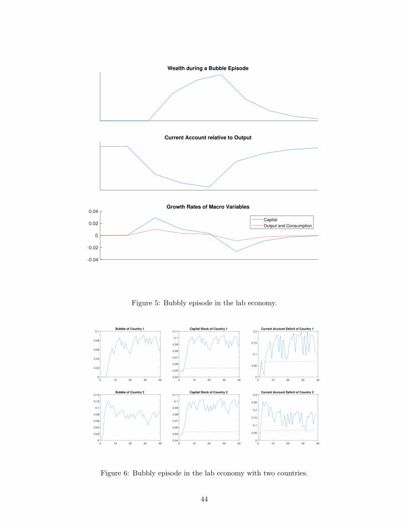
Wealth during a Bubble Episode

Current Account relative to Output

-0.04

-0.02

0

0.02

0.04Growth Rates of Macro Variables

Capital

Output and Consumption

Figure 5: Bubbly episode in the lab economy.

0 10 20 30 40

0.04

0.05

0.06

0.07

0.08

0.09

0.1

0.11

Capital Stock of Country 1

0 10 20 30 40

0

0.02

0.04

0.06

0.08

0.1

Bubble of Country 1

0 10 20 30 40

0

0.05

0.1

0.15

0.2

Current Account Deficit of Country 1

0 10 20 30 40

0.04

0.05

0.06

0.07

0.08

0.09

0.1

0.11

Capital Stock of Country 2

0 10 20 30 40

0

0.02

0.04

0.06

0.08

0.1

0.12

0.14

Bubble of Country 2

0 10 20 30 40

0

0.05

0.1

0.15

0.2

0.25

0.3

Current Account Deficit of Country 2

Figure 6: Bubbly episode in the lab economy with two countries.

44

References

[1] Abel, A. B. et al. (1989). Assessing Dynamic Effciency: Theory and Evidence. In: The Review

of Economic Studies 56.1, pp. 1-19.

[2] Aoki, K., T. Nakajima, and K. Nikolov (2014). Safe Asset Shortages and Asset Price Bubbles.

In: Journal of Mathematical Economics 53.C, pp. 164-174.

[3] Aoki, K. and K. Nikolov (2015). Bubbles, Banks and Financial Stability. In: Journal of Mo-

netary Economics 74, pp. 33-51.

[4] Arce, O. and D. Lopez-Salido (2011). Housing Bubbles. In: American Economic Journal:

Macroeconomics 3.1, pp. 212-241.

[5] Asriyan, V., L. Fornaro, A. Martin, and J. Ventura (2016). Monetary Policy for a Bubbly

World. In: National Bureau of Economic Research No. w22639.

[6] Azariadis, C. and B. D. Smith (1993). Adverse Selection in the Overlapping Generations Model:

the Case of Pure Exchange. In: Journal of Economic Theory 60.2, pp. 277-305.

[7] Barlevy, G., D. Gale, and F. Allen (2017). On Interest Rate Policy and Asset Bubbles. In:

2017 Meeting Papers, Society for Economic Dynamics.

[8] Basco, S. (2014). Globalization and Financial Development: A Model of the Dot-Com and the

Housing Bubbles . In: Journal of International Economics 92.1, pp. 78-94.

[9] Basco, S. (2016). Switching Bubbles: From Outside to Inside Bubbles. In: European Economic

Review 87, pp. 236 255.

[10] Beck, T., S. Claessens, S. Schmukler, et al. (2013). Financial globalization and crises: overview.

In: The Evidence and Impact of Financial Globalization, Elsevier Inc, pp. 1-12.

[11] Bengui, J. and T. Phan (2016). Asset Pledgeability and Endogenously Leveraged Bubbles. In:

mimeo, University of North Carolina at Chapel Hill.

[12] Bernanke, B. and M. Gertler (1989). Agency Costs, Net Worth, and Business Fluctuations.

In: The American Economic Review 79.1, pp. 14-31.

[13] Bernanke, B. and M. Gertler (2001). Should Central Banks Respond to Movements in Asset

Prices. In: The American Economic Review 91.2, pp. 253-257.

45

[14] Blanchard, O. J. (1979). Speculative Bubbles, Crashes and Rational Expectations. In: Econo-

mics letters 3.4, pp. 387-389.

[15] Blanchard, O. J. and M. W. Watson (1982). Bubbles, Rational Expectations and Financial

Markets. In: National Bureau of Economic Research, working paper.

[16] Blanchard, O. J. (1985). Debt, Deficits, and Finite Horizons. In: Journal of political Economy

93.2, pp. 223-247.

[17] Caballero, R. and A. Krishnamurthy (2006). Bubbles and Capital Flow Volatility: Causes and

Risk Management. In: Journal of Monetary Economics 53.1, pp. 33-53.

[18] Caballero, R. J., E. Farhi, and P.-O. Gourinchas (2008). An Equilibrium Model of Global

Imbalances and Low Interest Rates . In: The American Economic Review 98.1, pp. 358.

[19] Carvalho, V., A. Martin, and J. Ventura (2012). Understanding Bubbly Episodes. In: American

Economic Review 102.3, pp. 95-100.

[20] Coeurdacier, N., S. Guibaud, and K. Jin (2015). Credit Constraints and Growth in a Global

Economy. In: The American Economic Review 105.9, pp. 2838-2881.

[21] Diamond, P. A. (1965). National Debt in a Neoclassical Growth Model . In: The American

Economic Review 55.5, pp. 1126-1150.

[22] Diba, B. T. and H. I. Grossman (1988). The Theory of Rational Bubbles in Stock Prices. In:

The Economic Journal 98.392, pp. 746-754.

[23] Dong, F., J. Miao, and P. Wang (2017). Asset Bubbles and Monetary Policy. In: mimeo,

Boston University.

[24] Eichengreen, B. and M. D. Bordo (2002). Crises Now and Then: What Lessons from the Last

Era of Financial Globalization. In: National Bureau of Economic Research, working paper.

[25] Farhi, E. and J. Tirole (2012). Bubbly Liquidity. In: The Review of Economic Studies 79.2,

pp. 678-706.

[26] Freixas, X. and D. Perez-Reyna (2016). Gilded Bubbles. In: mimeo, Universitat Pompeu Fabra.

[27] Froot, K. and M. Obstfeld (1991). Intrinsic Bubbles: the Case of Stock Prices. In: American

Economic Review 81.5, pp. 1189-1214.

46

[28] Gali, J. (2014). Monetary Policy and Rational Asset Price Bubbles. In: The American Econo-

mic Review 104.3, pp. 721-752.

[29] Gali, J. (2017). Monetary Policy and Bubbles in a New Keynesian Model with Overlapping

Generations. In: mimeo, CREI.

[30] Geerolf, F. (2013). Reassessing Dynamic Effciency. In: mimeo, UCLA.

[31] Gopinath, G., et al. (2017). Capital allocation and productivity in South Europe. In: The

Quarterly Journal of Economics 132.4, pp. 1915-1967.

[32] Grossman, G. M. and N. Yanagawa (1993). Asset Bubbles and Endogenous Growth. In: Jour-

nal of Monetary Economics 31.1, pp. 3-19.

[33] Guerron-Quintana, P., T. Hirano, and R. Jinnai (2017). Recurrent Bubbles, Economic Fluc-

tuations and Growth. In: mimeo, Boston College.

[34] Gurkaynak, R. (2008). Econometric Tests of Asset Price Bubbles: Taking Stock. In: Journal

of Economic Surveys 22.1, pp. 166-186.

[35] Hanson, A., and T. Phan (2017). Bubbles, Wage Rigidity, and Persistent Recessions. In: Eco-

nomic Letters 151, pp. 66-70.

[36] Hirano, T., M. Inaba, and N. Yanagawa (2015). Asset Bubbles and Bailouts. In: Journal of

Monetary Economics 76, S71-S89.

[37] Hirano, T. and N. Yanagawa (2016). Asset Bubbles, Endogenous Growth, and Financial Fricti-

ons. In: The Review of Economic Studies 84.1, pp. 406-443.

[38] Huber, S. J. (2016). Preference for Housing Services and Rational House Price Bubbles. In:

mimeo, University of Amsterdam.

[39] Ikeda, D. (2017). Monetary Policy, Inflation and Rational Asset Price Bubbles. In: mimeo,

Bank of England.

[40] Ikeda, D., and T. Phan (2015). Asset Bubbles and Global Imbalances. In: mimeo, University

of North Carolina at Chapel Hill.

[41] Ikeda, D. and T. Phan (2016). Toxic asset bubbles . In: Economic Theory 2.61, pp. 241-271.

47

[42] Jorda, O., M. Schularick, and A. M. Taylor (2015). Leveraged Bubbles. In: Journal of Monetary

Economics 76, S1-S20.

[43] Jorda, O., M. Schularick, and A. M. Taylor (2017). Macro Financial History and the New

Business Cycle Facts. In: NBER Macroeconomics Annual 31.1, pp. 213-263.

[44] King, I. and D. Ferguson (1993). Dynamic Inefficiency, Endogenous Growth, and Ponzi Games.

In: Journal of Monetary Economics 32.1, pp. 79-104.

[45] Kiyotaki, N. and J. Moore (1997). Credit Cycles. In: Journal of Political Economy 105.2, pp.

211-248.

[46] Kocherlakota, N. (1992). Bubbles and constraints on debt accumulation. In: Journal of Eco-

nomic Theory 57.1, pp. 245-256.

[47] Kocherlakota, N. (2009). Bursting Bubbles: Consequences and Cures. In: mimeo, University

of Minnesota.

[48] Kraay, A. and J. Ventura (2007). The Dot-Com Bubble, the Bush Defcits, and the US Current

Account. In: G7 Current Account Imbalances: Sustainability and Adjustment, University of

Chicago Press, pp. 457-496.

[49] LeRoy, S. (2004). Rational Exuberance. In: Journal of Economic Literature 42.3, pp. 783-804.

[50] Martin, A. and J. Ventura (2011). Theoretical Notes on Bubbles and the Current Crisis. In:

IMF Economic Review 59.1, pp. 6-40.

[51] Martin, A. and J. Ventura (2012). Economic Growth with Bubbles. In: American Economic

Review 102.6, pp. 3033-3058.

[52] Martin, A. and J. Ventura (2015). The International Transmission of Credit Bubbles: Theory

and Policy. In: Journal of Monetary Economics 76, S37-S56.

[53] Martin, A. and J. Ventura (2016). Managing Credit Bubbles. In: Journal of the European

Economic Association 14.3, pp. 753-789.

[54] Miao, J. (2014). Introduction to Economic Theory of Bubbles. In: Journal of Mathematical

Economics 53, pp. 130-136.

48

[55] Miao, J. and P. Wang (2014). Sectoral Bubbles, Misallocation, and Endogenous Growth. In:

Journal of Mathematical Economics 53, pp. 153 163.

[56] Miao, J. and P. Wang (2015). Banking Bubbles and Financial Crises. In: Journal of Economic

Theory 157, pp. 763-792.

[57] Miao, J. and P. Wang (2016). Stock Market Bubbles and Unemployment. In: Economic Theory

61.2, pp. 273-307.

[58] Miao, J. and P. Wang (2017). Asset Bubbles and Credit Constraints. In: mimeo, Boston

University.

[59] Olivier, J. (2000). Growth-Enhancing Bubbles. In: International Economic Review 41.1, pp.

133-152.

[60] Queiros, F. (2017a). The Real Side of Stock Market Exuberance. In: mimeo, Universitat

Pompeu Fabra.

[61] Queiros, F. (2017b). Asset Bubbles and Product Market Competition. In: mimeo, Universitat

Pompeu Fabra.

[62] Rhee, C. (1991). Dynamic Inefficiency in an Economy with Land. In: The Review of Economic

Studies 58.4, pp. 791-797.

[63] Rondina, G. (2017). Bubbly Financial Globalization. In: mimeo, University of Colorado.

[64] Saint-Paul, G. (1992). Fiscal Policy in an Endogenous Growth Model. In: Quarterly Journal

of Economics 107.4, pp. 1243-1259.

[65] Samuelson, P. A. (1958). An Exact Consumption-loan Model of Interest with or without the

Social Contrivance of Money . In: The Journal of Political Economy 66.6, pp. 467 482.

[66] Schularick, M. and A. M. Taylor (2012). Credit Booms gone Bust: Monetary Policy, Leverage

Cycles, and Financial Crises, 1870 2008 . In: The American Economic Review 102.2, pp.

1029-1061.

[67] Tang, H. (2017). Asset Price Bubbles and the Distribution of Firms: A Theory of Economic

Expansions with an Application to Spain. In: mimeo, Universitat Pompeu Fabra.

49

[68] Tirole, J. (1985). Asset Bubbles and Overlapping Generations. In: Econometrica 53.6, pp.

1071-1100.

[69] Tripathy, J. (2017). Bubbly Equilibria with Credit Misallocation. In: mimeo, Universitat Pom-

peu Fabra.

[70] Ventura, J. (2012). Bubbles and Capital Flows. In: Journal of Economic Theory 147.2, pp.

738 758.

[71] Ventura, J. and H.-J. Voth (2015). Debt Into Growth: How Sovereign Debt Accelerated the

First Industrial Revolution. In: mimeo, CREI.

[72] Weil, P. (1987). Confidence and the Real Value of Money in Overlapping Generation Models.

In: Quarterly Journal of Economics 102.1, pp. 1-22.

[73] Woodford, M. (1990). Public Debt as Private Liquidity. In: The American Economic Review

80.2, pp. 382-388.

[74] Woodford, M. and M.S. Santos (1997). Rational asset pricing bubbles. In: Econometrica 65-1,

pp. 19-57.

[75] Yaari, M. E. (1965). Uncertain Lifetime, Life Insurance, and the Theory of the Consumer. In:

The Review of Economic Studies 32.2, pp. 137-150.

[76] Zhao, B. (2015). Rational Housing Bubble. In: Economic Theory 60.1, pp. 141-201.

50