The lukewarm frontier:

Some cosmological consequences of ‘low-energy’ physics

Thesis by

Daniel Grin

In Partial Fulfillment of the Requirements

for the Degree of

Doctor of Philosophy

California Institute of Technology

Pasadena, California

2010

(Defended May 28, 2010)

ii

c© 2010

Daniel Grin

All Rights Reserved

iii

“The effort to understand the universe is one of the very few things that lifts human life a little

above the level of farce, and gives it some of the grace of tragedy.”

– Steven Weinberg, 1993 [1]

“Our knowledge can only be finite, while our ignorance must necessarily be infinite.”

– Karl Popper, 1963 [2]

iv

Acknowledgments

My journey to and through graduate school was made possible and immeasurably more pleasant by

early nourishment, thoughtful mentorship, and the company of fellow travelers.

I begin by thanking my advisor, Prof. Marc Kamionkowski. Marc is rare in his deep curiosity

and broad-ranging interests as a cosmologist. I aspire to his scientific taste, to his example of how

to choose and solve problems. He has been a thoughtful advisor, pointing me to research problems

that are pedagogically and scientifically valuable, guiding me to cogent solutions, and reading my

manuscripts to help shape them into clear explanations of our work. He has been generous with his

time and his resources, allowing me to travel to fascinating conferences and summer schools. In this

difficult year for our department, he has exemplified availability and provided solace.

In the last two years, I have had the pleasure of collaborating with Prof. Chris Hirata, who has

generously shared his time, patience, and insight with me. Chris has acquainted me with the beauty

and cosmological utility of atomic physics and radiative transfer. Chris’s attention to detail and

ability to connect seemingly disparate areas of physics have inspired and guided me.

I thank my dedicated collaborators in the research presented in this thesis: Yacine Ali-Haımoud,

Andrew Blain, Robert Caldwell, Giovanni Covone, Chris Hirata, Eric Jullo, Marc Kamionkowski,

Jean-Paul Kneib, and Tristan Smith.

I thank Andrew Benson for introducing me to the rich physics behind dark matter halo and galaxy

formation, and for being a constructive sounding board for ideas and numerical experiments.

My father Leonid, mother Marina, and sister Rada never ceased believing in me, and I am deeply

grateful for their unwavering support, good humor, and reliable willingness to help. My earliest

memories involving science are of discovering science fiction, model rockets, and the night sky with

Marc Hoag, now my friend of 26 years. Marc lent me a copy of Kip Thorne’s book Black Holes

and Time Warps [3], planting my fascination with astrophysics. Thank you Kip for writing such an

inviting book. Kip’s lectures on general relativity and classical physics at Caltech were a paragon

of simplicity and clarity. It was a treat to TA for him. The teachers at Germantown Friends School

taught me the value of systematic thinking and hard work. My ninth grade biology teacher in

Los Gatos, John McDonald, taught me to embrace failure and strive for humility. My high-school

v

calculus teacher Jeanne-Marie Rachlin was exceptionally clear and supportive, helping me to begin

university math/physics courses with a running start. I’ve been lucky to call David Hembry a friend

for seventeen years. I continue to profit from thoughtful discourse with him about science, politics,

literature, and he has been a caring and supportive friend throughout. His diverse interests and wide

ken continue to inspire me. Aaron Silberstein has helped me to stay light-hearted and to appreciate

the fortune of my circumstances.

My professors and fellow physics students at Princeton helped lay the foundation for the fun I

had in graduate school. Zigmund Kermish taught us about the power of physical intuition (Ziggy is

always right) and was generous with his friendship. Tom Jackson relieved us with his understated

and brilliant humor. Erik Encarnacion (meta-physicist) never let us forget that a world of strife and

moral complexity exists outside the realm of gedankenexperimenten and laboratories.

Adrienne Erickcek and I did not finish squabbling over couch space at problem sessions during

our undergraduate years, so we followed one another to Great Britain and then Caltech. She has

been an attentive, caring, and insightful friend for eleven years, has cheered me at my best, but-

tressed me at my worst, and taught me to advocate for myself. I aspire to her diligence and insight

as a cosmologist. No one could ask for more from a friend or colleague.

Others at Caltech have contributed significantly to my well-being and academic progress. Tristan

Smith (the Park Ranger) has been a steadfast friend and a terrific travel partner in the Southwest.

He has been the first person I go to when I want to discuss a scientific idea or question. He has

always been willing to exchange new ideas and book suggestions, scientific and humanistic. I have

wonderful officemates. Nate Bode has shared wisdom, life experience, and stories of his gallant

voyages. Conversations with Nate are wonderful, be they about physics, music, or anything else,

because Nate doesn’t stop asking questions ’till he gets at the heart of the matter. Nate has also

made sure that I remember to occasionally look out the window. Yacine Ali-Haımoud has taught

me to never give up in the quest for an analytic solution, and I’ve enjoyed discussing the gory details

of recombination with him. He has been a good friend and brought levity to the office. Anthony

Pullen has been a model of diligence and efficiency, a fun study partner in first-year courses, and a

good-humored friend.

Anthony ‘Badgie’ Miller was a terrific roommate, tolerant of my forgetfulness, and indulgent of

my eccentricities. We enjoyed blasting classical music on his speakers and learned to love Los An-

geles together. Vaclav Cvicek followed in his stead, and he has kept me on my toes with late night

discussions in which I have to justify all of cosmology in five sentences or less. He’s also put up with

vi

my catastrophes in the kitchen, tumbling heavy objects, and has been a steadfast friend. Above all,

he has introduced me to Jara Cimrman’s externism.

I am thankful for the open-mindedness, and humility of Daniel Babich. Dan regularly took time to

share his problem-solving acumen and company with the graduate students in 158 Bridge.

I have enjoyed the wit and company of Hernan Garcia, Anusha Narayan, Jenny Roizen, usually

over lunch. I thank them for their patience with the etymological squabbles between Nate Bode and

me.

I am thankful for the friendship of all my fellow astronomy graduate students at Caltech. Spe-

cial thanks go to my incoming class: Ann Marie-Cody, Thiago Goncalves, and Hilke Schlichting. It

was always a pleasure to encounter Milan Bogosavljevic in the hallway. He reminded me to laugh

at myself with regularity. Karın Menendez-Delmestre has always taken the time to check in and say

a kind word.

Insofar as I am still sane, it is thanks to the distraction of music. Delores Bing runs a great chamber

music program at Caltech with grace and patience. It has been a privilege to perform music of

Beethoven, Brahms, Dvorak, Martinu, Messiaen, and Schubert in Dabney Lounge. I shared this

musical fun with my friends Jenelle Bray, Kevin Engel, Adrienne Erickcek, Nicholas Fette, George

Hines, Chris Kovalchick, Calvin Kuo, Yousi Ma, Anthony Miller, Hui Khoon Ng, Angela Shih, Jing

Shen, Lisa Tracy, Christina Vizcarra, Lillian Wang, Jackson Wang, Tina Wang, and June Wicks.

Delores has coached our chamber groups to successful performances many times over. The staff

at KUSC FM (above all Jim Svejda) have broadened my musical horizons and gotten me through

many a work-harried evening (and sunrise) with their thoughtful choices and commentary.

I am grateful to many others for their friendship during my time at Caltech: Lotty Ackerman,

Esfandiar Alizadeh, Mustafa Amin, Michael Armen, Doron Bergman, Laura Book, Mike Boyle, Jus-

tus Brevik, Geoff Chang, Michael Cohen, Ben Collins, Nicole Czakon, Chaim Danzinger, Natalie

Deffenbaugh, Tudor Dimofte, Olivier Dore, Vera Gluscevic, Leo Goldmakher, Daniel Haas, Lynn

Kamerlin, David Kantor, Jeff Kaplan, Matthew Kelley, Mike Kesden, David Kopp, Neil Halelamien,

Chaim Hanoka, Peggy Hsu, Elisabeth Krause, Zuli Kurji, Andy Lamperski, Nicholas Law, Sam Lee,

Michael Mendenhall, Diana Negoescu, David Nichols, Evan O’Connor, Rory Perkins, Annika Peter,

Harald Pfeiffer, Prof. Sterl Phinney, Paige Randall, Jonathan Pritchard, Christine Romano, John

Saunders, Prof. Re’em Sari, Iggy Sawicki, Mark Scheel, Kevin Setter, Kai Shen, Kris Sigurdson,

Brian Standley, Jenn Stockdill, Eve Stenson, Sherry Suyu, Aileen Tang, Kana Takematsu, Amanda

vii

Tavel, Ryan Trainor, Amy Trangsrud, Sarah Tulin, Sean Tulin, Tristan Ursell, Ramon van Handel,

and Todd Zoltan.

My research would grind to a halt were it not for the able and cheerful work of Caltech admin-

istrative staff, including Gina Armas, JoAnn Boyd, Helen Ticehurst, and Gita Patel. I owe special

thanks to Shirley Hampton, who made sure that recommendation letters arrived on time, and kept

the cosmology sub-group of TAPIR smoothly running. Chris Mach keeps the TAPIR computers

up and running, and saved me from near oblivion after an “rm -r *” crisis. I am grateful to the

staff of the Caltech Health Center, especially Maggie Ateia, Divina Bautista, Helena Kopecky, Alice

Sogomanian, and Paulette Theresa.

My deepest thanks go to my fiancee Sarah Tarlow. Her love, patience, and support have been

unwavering, unconditional, and indispensable. I will strive to fill our new home with warmth to

compensate for the dreary New Jersey weather.

viii

Abstract

In this thesis, we present four projects featuring low characteristic energy scales relative to the

scales relevant for supersymmetric dark matter production or inflation. We present a telescope

search for decaying relic axions in the 3−8 eV mass range. We utilize larger telescope exposure and

superior cluster mass modeling to improve sensitivity. Our results impose new stringent limits to

the two-photon coupling or relic density of axions. We extend these results to non-standard sterile

neutrinos.

We then reconsider cosmological constraints to axions. Our understanding of physics before

big-bang nucleosynthesis is tenuous, and after arguing that a non-standard thermal history before

nucleosynthesis is plausible and perhaps even natural, we calculate the abundance and typical mo-

menta of thermal axions in such scenarios. We generalize existing cosmological constraints to axions,

showing that the allowed axion mass range expands significantly in non-standard thermal histories.

We then estimate the sensitivity of future experiments to axion masses and reheating temperatures.

We then study the ∼ eV-scale physics of cosmological hydrogen recombination, computing the

recombination history while resolving all ∼ 104 states of hydrogen up to a maximum n ∼ 250 and

studying the associated convergence problem. We show that the recombination history is sufficiently

converged for analysis of microwave anisotropy data from the Planck satellite if the maximum

n ∼ 128, and that previously ignored electric quadrupole transitions are indeed negligible to the

precision necessary for Planck.

We conclude by presenting a new astrophysical limit to effective field theories of gravity in which

the graviton propagator is damped at energies greater than a milli-eV.

ix

Contents

Acknowledgments iv

Abstract viii

1 Introduction and Summary 1

2 A Telescope Search for Decaying Relic Axions 3

2.1 Introduction . . . . . . . . . . . . . . . . . . . . . . . . . . . . . . . . . . . . . . . . . 3

2.2 Theory . . . . . . . . . . . . . . . . . . . . . . . . . . . . . . . . . . . . . . . . . . . . 6

2.3 Constraints in the literature . . . . . . . . . . . . . . . . . . . . . . . . . . . . . . . . 17

2.4 Observations . . . . . . . . . . . . . . . . . . . . . . . . . . . . . . . . . . . . . . . . 20

2.4.1 Imaging Data . . . . . . . . . . . . . . . . . . . . . . . . . . . . . . . . . . . . 20

2.4.2 VIMOS Spectra . . . . . . . . . . . . . . . . . . . . . . . . . . . . . . . . . . 20

2.4.3 Reduction of IFU data . . . . . . . . . . . . . . . . . . . . . . . . . . . . . . . 22

2.5 Analysis . . . . . . . . . . . . . . . . . . . . . . . . . . . . . . . . . . . . . . . . . . . 25

2.5.1 Strong Lensing and Cluster Mass Maps . . . . . . . . . . . . . . . . . . . . . 25

2.5.2 Extraction of One Dimensional Spectra . . . . . . . . . . . . . . . . . . . . . 26

2.5.3 Limits on the two-photon coupling of axions . . . . . . . . . . . . . . . . . . . 29

2.5.4 Revision of past telescope constraints to axions . . . . . . . . . . . . . . . . . 32

2.5.5 Simulation of Analysis Technique . . . . . . . . . . . . . . . . . . . . . . . . . 33

2.5.6 Cross-Correlation Analysis . . . . . . . . . . . . . . . . . . . . . . . . . . . . 34

2.5.7 Sterile neutrinos . . . . . . . . . . . . . . . . . . . . . . . . . . . . . . . . . . 37

2.5.8 Ongoing Work . . . . . . . . . . . . . . . . . . . . . . . . . . . . . . . . . . . 38

2.6 Conclusions . . . . . . . . . . . . . . . . . . . . . . . . . . . . . . . . . . . . . . . . . 39

3 Thermal axion constraints in non-standard thermal histories 41

3.1 Introduction . . . . . . . . . . . . . . . . . . . . . . . . . . . . . . . . . . . . . . . . . 41

3.2 Two non-standard thermal histories: Low-temperature reheating and kination . . . . 46

3.3 Axion production in non-standard thermal histories . . . . . . . . . . . . . . . . . . 48

3.4 Constraints to axions . . . . . . . . . . . . . . . . . . . . . . . . . . . . . . . . . . . . 52

3.4.1 Constraints to the axion mass from Ωmh2 . . . . . . . . . . . . . . . . . . . . 55

3.4.2 Constraints to the axion mass from CMB/LSS data . . . . . . . . . . . . . . 55

3.5 Axions as relativistic degrees of freedom at early times . . . . . . . . . . . . . . . . . 59

x

3.6 Conclusions . . . . . . . . . . . . . . . . . . . . . . . . . . . . . . . . . . . . . . . . . 61

4 Cosmological hydrogen recombination: The effect of extremely high-n states 64

4.1 Introduction . . . . . . . . . . . . . . . . . . . . . . . . . . . . . . . . . . . . . . . . . 64

4.2 The standard multilevel atom . . . . . . . . . . . . . . . . . . . . . . . . . . . . . . . 68

4.2.1 Basic framework . . . . . . . . . . . . . . . . . . . . . . . . . . . . . . . . . . 68

4.2.2 Radiative transfer and escape probabilities . . . . . . . . . . . . . . . . . . . 70

4.2.2.1 Line overlap . . . . . . . . . . . . . . . . . . . . . . . . . . . . . . . 71

4.2.3 Matter and radiation temperatures . . . . . . . . . . . . . . . . . . . . . . . . 73

4.2.4 The steady-state approximation . . . . . . . . . . . . . . . . . . . . . . . . . . 74

4.3 Recombination with high-n states . . . . . . . . . . . . . . . . . . . . . . . . . . . . . 75

4.3.1 Are high-n states well-defined and physical? . . . . . . . . . . . . . . . . . . . 76

4.3.2 Computational challenges . . . . . . . . . . . . . . . . . . . . . . . . . . . . . 80

4.3.3 Rates . . . . . . . . . . . . . . . . . . . . . . . . . . . . . . . . . . . . . . . . 80

4.3.3.1 Bound-bound rates . . . . . . . . . . . . . . . . . . . . . . . . . . . 81

4.3.3.2 Bound-free rates . . . . . . . . . . . . . . . . . . . . . . . . . . . . . 82

4.3.4 Sparse-matrix technique . . . . . . . . . . . . . . . . . . . . . . . . . . . . . . 83

4.3.5 Numerical methods . . . . . . . . . . . . . . . . . . . . . . . . . . . . . . . . . 86

4.4 Extension to electric quadrupole transitions . . . . . . . . . . . . . . . . . . . . . . . 86

4.4.1 Rates . . . . . . . . . . . . . . . . . . . . . . . . . . . . . . . . . . . . . . . . 87

4.4.2 Inclusion in multilevel atom code . . . . . . . . . . . . . . . . . . . . . . . . . 88

4.5 Results . . . . . . . . . . . . . . . . . . . . . . . . . . . . . . . . . . . . . . . . . . . . 89

4.5.1 State of the gas . . . . . . . . . . . . . . . . . . . . . . . . . . . . . . . . . . . 89

4.5.1.1 Populations of angular momentum sublevels . . . . . . . . . . . . . 89

4.5.1.2 The effect of collisions . . . . . . . . . . . . . . . . . . . . . . . . . . 91

4.5.1.3 Populations of Rydberg energy levels . . . . . . . . . . . . . . . . . 96

4.5.2 Population inversion in the primordial plasma . . . . . . . . . . . . . . . . . . 98

4.5.3 The effect of extremely high-n states on recombination histories . . . . . . . . 102

4.5.4 Code comparisons . . . . . . . . . . . . . . . . . . . . . . . . . . . . . . . . . 103

4.5.5 The effect of high-n states on CMB anisotropies . . . . . . . . . . . . . . . . 106

4.5.5.1 The visibility function . . . . . . . . . . . . . . . . . . . . . . . . . . 108

4.5.6 Statistical significance of corrections to the recombination history . . . . . . . 112

4.5.7 The effect of electric quadrupole transitions on recombination histories and

the CMB . . . . . . . . . . . . . . . . . . . . . . . . . . . . . . . . . . . . . . 113

4.6 Conclusions . . . . . . . . . . . . . . . . . . . . . . . . . . . . . . . . . . . . . . . . . 118

5 Lower Limit to the Scale of an Effective Theory of Gravitation 121

xi

A King/NFW surface density profiles 128

B The effect of updated cluster mass-profiles on constraints obtained from A1413,

A2256, and A2218 129

C WKB approximation for radial dipole integrals 132

D Radial bound-bound quadrupole integrals 134

xii

List of Figures

2.1 Electric dipole moment of a neutron. . . . . . . . . . . . . . . . . . . . . . . . . . . . 7

2.2 Axions couple to photons via PQ+electromagnetically charged Dirac fermions. . . . 10

2.3 Axions couple to photons via mixing with pions. . . . . . . . . . . . . . . . . . . . . 10

2.4 Axions acquire mass by mixing with pions. . . . . . . . . . . . . . . . . . . . . . . . 11

2.5 Allowed axion parameter space, compiled from many experiments. . . . . . . . . . . 17

2.6 Allowed axion parameter space if axion two-photon coupling vanishes. . . . . . . . . 21

2.7 Image of the galaxy cluster Abell 2667 (A2667) with overlaid strong-lensing contours. 22

2.8 Image of the galaxy cluster Abell 2390 (A2390) with overlaid strong-lensing contours. 23

2.9 Surface mass density map of A2667. . . . . . . . . . . . . . . . . . . . . . . . . . . . 26

2.10 Surface mass density map of A2390. . . . . . . . . . . . . . . . . . . . . . . . . . . . 27

2.11 Average one-dimensional sky subtracted spectra of clusters A2667 and A2390. . . . . 29

2.12 Constraints on intensity/surface density ratio 〈Iλ/Σ12〉. . . . . . . . . . . . . . . . . 30

2.13 Upper limits to the two-photon coupling parameter ξ of the axion. . . . . . . . . . . 33

2.14 Comparison of existing limits to ξ with past and estimated future limits to ξ. . . . . 35

2.15 Limits on the combination ξ(

Ωah2)1/2

. . . . . . . . . . . . . . . . . . . . . . . . . . 36

2.16 Slice of simulated IFU data cube. . . . . . . . . . . . . . . . . . . . . . . . . . . . . . 37

2.17 Cross-correlation g(l) between spectra of A2667 and A2390. . . . . . . . . . . . . . . 38

3.1 Temperature T (a) as a function of scale factor, in a low-temperature reheating (LTR)

scenario. . . . . . . . . . . . . . . . . . . . . . . . . . . . . . . . . . . . . . . . . . . . 48

3.2 Hubble parameter H(T ) and radiation/matter energy densities as a function of tem-

perature, in a LTR scenario. . . . . . . . . . . . . . . . . . . . . . . . . . . . . . . . . 49

3.3 Thermal axion freeze-out temperature TF as a function of the reheating temperature

Trh, in a LTR scenario. . . . . . . . . . . . . . . . . . . . . . . . . . . . . . . . . . . . 50

3.4 Axion abundance Ωa as a function of Trh, in a LTR scenario. . . . . . . . . . . . . . 53

3.5 Upper limit to the axion mass from the evolution of horizontal branch (HB) stars in

globular clusters. Limits are shown as a function of the up/down quark mass ratio

r = mu/md, for four different axion models, parameterized by the value of E/N . The

region above the line is excluded, while below the line is allowed. Limits to ga→γγ are

taken from Refs. [4, 5] and generalized to varying r and E/N . . . . . . . . . . . . . . 54

3.6 Cosmological upper limits to thermal axion mass ma as a function of Trh, in a LTR

scenario. . . . . . . . . . . . . . . . . . . . . . . . . . . . . . . . . . . . . . . . . . . . 56

xiii

3.7 Origin of LSS limits to axions, from Ref. [6]. . . . . . . . . . . . . . . . . . . . . . . 57

3.8 Estimated improvement of accessible thermal axion parameter space in LTR scenarios,

with future observations. . . . . . . . . . . . . . . . . . . . . . . . . . . . . . . . . . . 59

3.9 Effective neutrino number N effν as a function of reheating temperature Trh for 3 dif-

ferent axion masses. . . . . . . . . . . . . . . . . . . . . . . . . . . . . . . . . . . . . 61

3.10 Axion parameter space in LTR scenarios accessible through future measurements of

the 4He mass fraction Yp. . . . . . . . . . . . . . . . . . . . . . . . . . . . . . . . . . 62

4.1 Evolution of the ratio of matter/radiation temperatures TM/TR as a function of red-

shift z. . . . . . . . . . . . . . . . . . . . . . . . . . . . . . . . . . . . . . . . . . . . . 74

4.2 Shell numbers at which stimulated emission, Debye screening, and collisions begin to

significantly broaden Hydrogen energy levels. . . . . . . . . . . . . . . . . . . . . . . 79

4.3 Schematic of the sparse rate matrix T. . . . . . . . . . . . . . . . . . . . . . . . . . . 84

4.4 Deviations from statistical equilibrium between different l states for z ' 1301, 1391,

and 1488. . . . . . . . . . . . . . . . . . . . . . . . . . . . . . . . . . . . . . . . . . . 90

4.5 Deviations from statistical equilibrium between different l states for z ' 555, 835,

and 1255. . . . . . . . . . . . . . . . . . . . . . . . . . . . . . . . . . . . . . . . . . . 91

4.6 The effect of l = 2 Balmer lines on the populations of different l states. . . . . . . . . 92

4.7 Ratio of radiative to collisional depopulation rates of the n = 150 energy shell. . . . 94

4.8 Ratio of radiative to collisional depopulation rates of the n = 50 energy shell. . . . . 95

4.9 Importance of collisions as a function of redshift . . . . . . . . . . . . . . . . . . . . 96

4.10 Populations of atomic hydrogen energy shells as a function of n, compared to values

in Boltzmann equilibrium with n = 2, for z ' 555, 631, 835, and 1255. . . . . . . . . 97

4.11 Populations of atomic hydrogen energy shells as a function of n, compared to values

in Saha equilibrium with the continuum, for z ' 555, 631, 835, and 1255. . . . . . . 98

4.12 Populations of atomic hydrogen energy shells as a function of z, compared to values

in Saha equilibrium with the continuum, for n = 48, 71, and 94. . . . . . . . . . . . 99

4.13 Population inversion between the n = 49 and n′ = 50 energy levels. . . . . . . . . . . 103

4.14 Recombination histories xe(z) as a function of nmax. . . . . . . . . . . . . . . . . . . 104

4.15 Convergence of relative errors in recombination histories xe(z) as a function of nmax. 105

4.16 Comparison of RecSparse output for xe(z) with results of Chluba et. al . . . . . . 106

4.17 Convergence of recombination histories in Refs. [7–9]. . . . . . . . . . . . . . . . . . 107

4.18 Effect of successively higher values of nmax on the CMB temperature anisotropy power

spectrum (CTT` ). . . . . . . . . . . . . . . . . . . . . . . . . . . . . . . . . . . . . . . 109

4.19 Effect of successively higher values of nmax on the CMB E-mode polarization anisotropy

power spectrum (CEE` ). . . . . . . . . . . . . . . . . . . . . . . . . . . . . . . . . . . 110

xiv

4.20 Effect of high-n states on the visibility function. . . . . . . . . . . . . . . . . . . . . . 111

4.21 Effect of E2 quadrupole transitions in atomic hydrogen on recombination history xe(z).114

4.22 Schematic indicating the effect of quadrupole transitions with n < 5 on the early

cosmic recombination history. . . . . . . . . . . . . . . . . . . . . . . . . . . . . . . . 115

4.23 Schematic indicating the effect of quadrupole transitions with n ≥ 5 on the early

cosmic recombination history. . . . . . . . . . . . . . . . . . . . . . . . . . . . . . . . 116

4.24 Schematic indicating the effect of quadrupole transitions with any n on the late cosmic

recombination history. . . . . . . . . . . . . . . . . . . . . . . . . . . . . . . . . . . . 117

4.25 Effect of E2 quadrupole transitions in atomic hydrogen on the CMB temperature

anisotropy power spectrum (CTT` ). . . . . . . . . . . . . . . . . . . . . . . . . . . . . 118

4.26 Effect of E2 quadrupole transitions in atomic hydrogen on the CMB E-mode polar-

ization anisotropy power spectrum (CEE` ). . . . . . . . . . . . . . . . . . . . . . . . . 119

5.1 Feynman diagrams for light deflection. . . . . . . . . . . . . . . . . . . . . . . . . . . 123

xv

List of Tables

2.1 Upper limits to line intensity and ξ. . . . . . . . . . . . . . . . . . . . . . . . . . . . 34

2.2 Upper limits to ξ obtained using cross-correlation method. . . . . . . . . . . . . . . . 39

B-1 Summary of observations and cluster properties in Refs. [10, 11]. . . . . . . . . . . . 130

B-2 Best-fit parameters for the mass model of A2218, determined from a strong-lensing

analysis. . . . . . . . . . . . . . . . . . . . . . . . . . . . . . . . . . . . . . . . . . . . 131

1

Chapter 1

Introduction and Summary

Modern cosmology offers an embarrassment of riches. Thanks to projects like BOOMERANG [12],

COBE [13], WMAP [14–17], the 2dF/SDSS surveys [18–21], the High-Z supernova search, and the

Supernova Cosmology Project [22–25], cosmology has become a precise science. Our understanding

of the universe’s contents and history is impressive. We know that the universe is flat, that its

matter content is dominated by non-baryonic dark matter, and that its baryonic content suffices to

explain light-element abundances. We know that the cosmological energy budget was dominated by

radiation for temperatures T ≤ 4 MeV [26], that the cosmological expansion is accelerating ‘today,’

and that the initial density perturbations were nearly scale-invariant, Gaussian, and adiabatic. These

are the riches of modern cosmology.

They are also its embarrassments. We do not know which (if any) of the particles in the myriad

of proposed extensions to the standard model (SM) of particle physics constitutes the dark matter,

although axions, weakly interacting massive particles (WIMPs) and sterile neutrinos are a few

plausible candidates. We have no firm anchor on the cosmological expansion history prior to big-

bang nucleosynthesis (BBN), though the observed spectrum of density fluctuations is consistent with

an early inflationary epoch. If the universe inflates, we must still identify the responsible field(s)

(the inflatons). There is no satisfying fundamental explanation of the apparent milli-eV energy scale

of the current cosmological acceleration.

Fortunately, ongoing and future planned experiments/surveys promise to break this impasse.

The ADMX/CAST [27, 28] experiments continue to search for dark matter/solar axions. Telescope

axion searches are chipping away at the thermal axion window. Experimental searches based on

axion-nucleon couplings and cosmological large-scale structure surveys should probe a wide range of

axion masses more definitively. In the case of WIMP dark matter, the trifecta of the Large Hadron

Collider (LHC) [29, 30], the Fermi γ-ray space telescope [31], and direct detection experiments like

CDMS/ZEPLIN/XENON [32–34] offer the possibility of detecting super-symmetric partners in the

lab and then confirming their identity as the dark matter. The recently launched Planck satellite will

begin to meaningfully test inflationary models through extremely precise measurements of cosmic

microwave background (CMB) anisotropies [35].

Much of the mystery and future promise in cosmology has to do with physics at several famous

high energy scales:

1. The Planck scale: mpl ∼ 1019 GeV. This is the putative scale at which string theory (or

2

any theory of quantum gravity) becomes relevant. The inflaton and cosmologically dominant

moduli fields may emerge from string theory.

2. The GUT (grand unified theory) scale: EGUT ∼ 1016 GeV. This scale may be relevant for

inflationary physics and baryogenesis.

3. The Peccei-Quinn scale [36]: 107 GeV ∼< fa ∼< 1012 GeV. If the dark matter is an axion or a

saxion, this scale will be relevant for dark matter physics.

4. The electroweak scale: E ∼ 250 GeV. If the dark matter is a neutralino or a gravitino, this

scale will be relevant for understanding the dark matter. This scale may also be important in

models of the origin of the cosmic baryon asymmetry.

Experimental and observational leverage on this physics, however, passes to us through a lower

energy filter. To understand the axion, inflation, and the CMB, we must deal with the ∼ 5 eV

energies accessible to optical telescopes, the ∼ 10 − 100 MeV temperatures preceding BBN (when

thermal axions fall out of chemical equilibrium), the ∼ eV temperature at matter-radiation equality

(when density perturbations begin to grow), and the ∼ 0.25 eV temperatures at photon-baryon de-

coupling. If care is not taken in modeling the recombination of the primordial plasma (the formation

of the first hydrogen atoms), inferences about the early universe made using data from Planck or

other next-generation CMB experiments (e,g., CMBPol [37]) should not be trusted: the experimen-

tal error bars will be comparable to or smaller than corrections that result from using a more precise

atomic physics model of recombination [38–41]. In the case of the cosmic acceleration, new physics

seems to kick in at the milli-eV energy scale.

In this thesis, we present several research projects in which these lower energy scales feature

prominently. Results from a new telescope search for decaying thermal axions are presented in

Chapter 2, along with extensions to non-standard sterile neutrinos and an implication for the early

thermal history of the universe. In Chapter 3, we determine the effect of late-time entropy gen-

eration in the range 10 MeV < T < 100 MeV and kination models on thermal axion production

and cosmological axion constraints. Chapter 4 features new computations of cosmological hydrogen

recombination including ∼ 104 states of the Rydberg atom and a tower of electric quadrupole tran-

sitions in atomic hydrogen. We compute and discuss the effects of this physics on CMB anisotropies

and parameter estimation, compare our results with other recent work, and describe a series of on-

going and future extensions of this work. In Chapter 5, we present an astrophysical limit to ‘fading’

effective field theories of gravity.

The bulk of our work in each chapter has been published in refereed journals and is reproduced

here with permission: Chapter 2 in Ref. [42], Chapter 3 in Ref. [43], Chapter 4 in Ref. [44], and

Chapter 5 in Ref. [45]. Additional pedagogical or introductory material has been added, as have

several new results. New material is pointed out at the beginning of each chapter.

3

Chapter 2

A Telescope Search for Decaying Relic

Axions1

2.1 Introduction

Axions are an obvious dark-matter candidate in some of the most conservative extensions of the

standard model of particle physics. The magnitude of the charge-parity (CP) violating term in

quantum chromodynamics (QCD) is tightly constrained by experimental limits to the electric dipole

moment of the neutron, presenting the strong CP problem [46–49]. Fine tuning can be avoided

through the Peccei-Quinn (PQ) mechanism, in which a new symmetry (the Peccei-Quinn symmetry)

is introduced, along with a new pseudoscalar particle, the axion. These ingredients dynamically drive

the CP violating term to zero [4, 36, 50]. Via mixing with pions, axions pick up a mass, which is

set by the PQ scale [4].

Below a mass of 10−2 eV, axions will be produced through coherent oscillations of the PQ

pseudoscalar, yielding a population of cold relics that dominate the dark-matter density [50–52].

Above this mass, axions will be in thermal equilibrium at early times [50, 51]. Unless ma ∼> 15 eV,

the resulting relic density is insufficient to account for all the dark matter, but high enough that

axions will be a nontrivial fraction of the dark matter and likely constitute a larger fraction of the

mass density of the universe than either baryons or neutrinos [50]! In either case, axions might be

detectable through their couplings to standard-model particles.

The couplings of the axion are set by the PQ scale and the specific axion model [4, 50, 53].

In the Dine-Fischler-Srednicki-Zhitnitski (DFSZ) axion model, standard-model fermions (quarks

and leptons) carry PQ charge, and so axions couple to photon pairs both via electrically charged

standard-model leptons and via mixing with pions [54, 55]. In hadronic axion models, such as the

Kim-Shifman-Vainshtein-Zakharov (KSVZ) axion model [56, 57], axions do not couple to standard-

model leptons at tree level. Indeed, in the KSVZ model itself, axions do not even couple to standard

model quarks. In KSVZ models, axions couple to gluons through triangle diagrams involving exotic

fermions, to pions via gluons, and to photons via mixing with pions.

Constraints to the two-hadron couplings of axions come from stellar evolution arguments, from

the duration of the neutrino burst from SN1987a, and from the upper limit to their cosmological

1The material in this chapter was adapted from Telescope search for decaying relic axions, Daniel Grin andothers; Phys. Rev. D 75, 105018 (2006). Reproduced here with permission, copyright (2006) by the AmericanPhysical Society. Additional material has been added in Sec. 2.2 and 2.3.

4

density [4, 50, 58–62]. Upper limits to the two-photon coupling of the axion come from searches for

solar axions [63], from upper limits to the intensity of the diffuse extragalactic background radiation

(DEBRA) [51, 64], from stellar evolution arguments [4], from direct searches for cosmic axions [27]

and from upper limits to x-ray and optical emission by galaxies and clusters of galaxies [10, 11, 51].

Recent searches for vacuum birefringence report evidence for the existence of a light boson [65–71],

though in a region of parameter space already constrained by null solar axion searches [63, 72, 73].

The two-photon coupling of the axion will lead to monochromatic line emission from axion decays

to photon pairs. Although the lifetime of the axion is much longer than a Hubble time, the dark-

matter density in a galaxy cluster is sufficiently high that optical line emission due to the decay of

cluster axions could be detected. This line emission should trace the density profile of the galaxy

cluster. Telescope searches for this emission were first suggested in Ref. [74]. In Ref. [51], this

suggestion was extended to thermally produced axions. A telescope search for this emission was

first attempted in Refs. [10, 11], in which a null search imposed upper limits to the two-photon

coupling of the axion in the mass window 3 eV ≤ ma ≤ 8 eV. Less stringent constraints have been

obtained in searches for decaying galactic axions [10, 75].

In the past few years, high-precision cosmic microwave background (CMB) and large-scale-

structure (LSS) measurements have become available and allowed new constraints to axion pa-

rameters in this mass range. In particular, axions in the few-eV mass range behave like hot dark

matter and suppress small-scale structure in a manner much like neutrinos of comparable masses.

Reference [6] shows that such arguments lead to an axion-mass bound ma ≤ 1.05 eV. Still, given

uncertainties and model dependences, it is important in cosmology to have several techniques as

verification. For example, in extended, low-temperature (∼ MeV) reheating models [76–78], light

relics like axions and neutrinos have suppressed abundances, evading CMB/LSS bounds, but may

still show up in telescope searches for axion decay lines [43]. Finally, other dark-matter candidates

may show up in such searches; the sterile neutrino [79–82] is one example, which we will discuss be-

low. We are thus motivated to re-visit the searches of Refs. [10, 11] and see whether new telescopes,

techniques, and observations may yield improvements.

Refs. [10, 11] preceded the advent of observations of gravitational lensing by galaxy clusters,

however, and so the cluster mass density profiles assumed were not measured directly, but derived

using x-ray data and assumptions about the dynamical state of the clusters. The constraints reported

in Refs. [10, 11] depend on these assumptions. Today, gravitational-lensing data can be used to

determine cluster density profiles, independent of dynamical assumptions [83]. Thus, by using lensing

mass maps and by applying the larger collecting areas of modern telescopes, cluster constraints

to axions can both be tightened, and made robust. The high spatial resolution of integral field

spectroscopy allows the use of lensing mass maps to extract the component of intracluster emission

that traces the cluster mass profile. Cluster mass models can be used to derive an optimal spatial

5

weighting of the data, thus focusing on parts of the cluster where the highest signal is expected.

To this end, we have conducted a search for optical line emission from the two-photon decays

of thermally produced axions.2 We used spectra of the galaxy clusters Abell 2667 (A2667) and

Abell 2390 (A2390) obtained with the Visible Multi-Object Spectrograph (VIMOS) Integral Field

Unit (IFU), which has the largest field of view of any instrument in its class [84]. VIMOS is a

spectrograph mounted at the third unit (Melipal) of the Very Large Telescope (VLT), part of the

European Southern Observatory (ESO) in Chile [85]. In our analysis, we use mass models of the

clusters derived from strong-lensing data, obtained with the Hubble Space Telescope (HST), using

the Wide Field Planetary Camera #2 (WFPC-2).

We obtain new upper limits to the two-photon coupling of the axion in the mass window 4.5 eV ≤ma ≤ 7.7 eV (set by the usable wavelength range of the VIMOS IFU) of ξ ≤ 0.003− 0.017. The

two-photon coupling of the axion, ξ, is defined in Eq. (2.13) and discussed in Section 2.2. Although

we search a smaller axion mass range than Refs. [10, 11], our upper limits improve on past work

by a factor of 2.1− 7.1, depending on the candidate axion mass and how the limits of Ref. [10, 11]

are rescaled to correct for today’s best-fit cosmological parameters and more accurate cluster mass

profiles. Our data rule out standard hadronic and DFSZ models in the 4.5 eV − 7.7 eV window.

However, theoretical uncertainties in quark masses and pion couplings may allow for a much wider

range of values of ξ than standard hadronic and DFSZ models allow, as emphasized by Ref. [86],

thus motivating the search for axions with smaller values of ξ.

A quick estimate shows that our level of improvement is not unexpected: the collecting area of

the VLT is a factor of (8.1/2.1)2 greater than the 2.1m telescope at Kitt Peak National Observatory

(KPNO) used in Ref. [11]. Our integration time is a factor of 10.8 ksec/3.6 ksec greater. The IFU

allows us to cover 3.4 times as much of the field of view as the spectrographs used at KPNO. Thus

we estimate that our collecting area should be a factor of ∼ 160 higher than that of Ref. [11]. If

there is no signal, and if we are noise limited, we would expect a constraint to flux that is a factor

of ' 13 more stringent than that of Ref. [11], and, since Iλ ∝ ξ2, upper limits to ξ that are ' 3.5

times more stringent than those reported in Ref. [11].

We begin by reviewing the relevant theory and proceed to describe our observations. We then

summarize our data analysis technique. The new limits to axion parameter space are then discussed

along with other constraints. We conclude by pointing out the potential of conducting such work

with higher redshift clusters. For consistency with the assumptions used to derive the strong-lensing

maps used in our analysis, we assume a ΛCDM cosmology parameterized by h = 0.71, Ωm = 0.30,

and ΩΛ = 0.70, except where explicitly noted otherwise.

2Based on observations made with ESO Telescopes at the Paranal Observatories (program ID 71.A-3010), andon observations made with the NASA/ESA Hubble Space Telescope, obtained from the data archive at the SpaceTelescope Institute. STScI is operated by the association of Universities for Research in Astronomy, Inc. under theNASA contract NAS5-26555.

6

2.2 Theory

Axions were postulated in 1977 to solve the ‘strong-CP’ problem [36, 87, 88]. The weak sector has

long been know to violate CP (charge-parity) symmetry, specifically through the decays of neutral

kaons and B-mesons. No CP-violation has been detected in the strong sector, although no symmetry

(gauge or global) prevents one from adding a term of the form [46, 89]

Lθ = − g2s

64π2θεµνρκG

pµνGρκp = − g2

s

32π3θGpGp (2.1)

to the standard model (SM) Lagrangian, where gs is the strong coupling constant and θ is a dimen-

sionless constant. Here εµνρκ is the usual Levi-Civita tensor and Gpµν = εµνρκGpρκ is the dual of

the gluon field-strength tensor. Roman indices (e.g. p) denote QCD color indices, and a pair of up-

down repeated indices denotes a sum, as per the usual Einstein convention. Although such surface

terms are irrelevant to the dynamics of Abelian gauge theories, they turn out to correspond to an

unconserved current (the axial vector current, to be precise) in theories with a local non-Abelian

gauge symmetry, once the theory is regularized [46, 90].

This ‘because-we-can’ addition to the Lagrangian may seem logically wanting, but it turns out

that tunneling between the many degenerate vacua of QCD (which must be formally included

when evaluating matrix elements) naturally leads to an effective Lagrangian term of the form in

Eq. 2.1, where the physical QCD vacuum is |θ〉 =∑∞

n=−∞ e−inθ|n〉 and 0 ≤ θ ≤ 2π [4, 46]. It

is a straightforward exercise to see that terms proportional to F F or GG are CP-violating (recall

that Fµν = εµνρκFρκ, where Fρκ is the usual Maxwell field tensor from electromagnetism). It turns

out that one physical consequence of a θ-term in QCD is the prediction of a nonzero electric-dipole

moment for the neutron, given by dn ∼ 10−15 e cm, where e is the charge of of an electron [4, 47, 48].

If we imagine a toy model of a neutron, as two classical oppositely charged current loops, we see

that under a CP transformation (switch the charges and reverse the directions of each current), the

electric field points in the opposite direction while the magnetic field is unchanged. In other words,

a neutron electric dipole moment violates CP, as does any term of the form ~E · ~B, as we can see in

Fig. 2.1. Experimental limits impose the constraint dn ≤ 6 × 10−26 e cm, and so θ < 10−10, even

though one might naively expect this phase to be of order unity.

Moreover, when the weak-sector quark mass matrix M is diagonalized and made real through

SU(2) rotations and phase transformations (to identify physical mass eigenstates), an additional

term of the form in Eq. 2.1 results, and so the physical variable relevant to dn is in fact θ =

θ − arg det M [4]. Since θ and M correspond to physics in the distinct strong and weak sectors,

respectively, the near-vanishing of θ would require considerable fine tuning. In the spirit of solutions

to other fine tuning problems, Peccei and Quinn proposed making θ into a dynamical field ζ, with

a degenerate vacuum corresponding to a new global [Peccei-Quinn (PQ)] U(1) symmetry [36].

7

LCPV = 2GG

E B E B

CP

Figure 2.1 Toy model of a neutron as two classical oppositely charged current loops. Under a CPtransformation, the electric field flips directions, while the magnetic field stays pointed in the samedirection. Thus a neutron electric dipole moment violates CP symmetry.

When the physical vacuum is set by spontaneous symmetry breaking (with vacuum expectation

value v/√

2), we get a new Goldstone boson φ corresponding to the phase of the complex scalar

[36, 87, 88]. In the free field theory for ζ, φ would be an unconstrained flat direction, but couplings

of the form ζGG will introduce classical dynamics for φ that drive the net CP-violating phase to

zero. Quantum fluctuations in φ would correspond to a new particle, the axion [88].

As we shall see below, axion couplings are proportional to fπ/fa, where fa is the symmetry-

breaking scale. It was originally hoped that the axion might be the Goldstone boson of a two-

component Higgs (a very modest extension of the SM), with fa ∼ fEW, where the electroweak scale

fEW ∼ 102 GeV, but this possibility was quickly ruled out by accelerator experiments [4, 91]. In

its place, we have the invisible axion hypothesis, in which fa fEW, giving the axion extremely

weak couplings. Since fa could a priori span the huge range of scales fEW < fa < MPl (where

mPl ∼ 1019 GeV is the Planck mass), it is hard work to scan through axion parameter space.

Axion decay rates to photons in galaxy clusters will of course depend on the couplings of the

axion. We can understand axion couplings (and masses) using hadronic axion models and then

generalize to a larger family of models by expanding the set of allowed quantum numbers. In this

discussion, we follow closely the formalism for axion couplings laid out in Ref. [89]. In a hadronic

axion model, there is a new complex scalar ζ which carries PQ charge 2 and has a potential V (ζ).

There is also a family ψi of new Dirac fermions (i ∈ 1, N for some N), each of which transforms as

a triplet under QCD SU(3) (in other words, the new heavy fermions have standard QCD interactions

but also carry PQ charge). The new fermions are given mass through Yukawa interaction terms, that

is, we have terms of the form yiψi

LζψiR in the Lagrangian, where the yi are the Yukawa couplings and

ψ ≡ ψ†γ0. Here we have the standard Dirac matrices γµ from the SM along with γ5 = iγ0γ1γ2γ3,

8

as well as the usual projections onto left and right-handed spinors [90]:

ψiL =

1

2

(

1− γ5)

ψi,

ψiR =

1

2

(

1 + γ5)

ψi. (2.2)

The full Lagrangian density for the hadronic model then reads [89]

L = LSM + Lkin −∑

i

yi

(

ψi

LζψiR + Hermitian conjugate

)

− V (ζ)− g2s

32π2θGpµνGpµν , (2.3)

where LSM is the complete SM Lagrangian density. When the PQ symmetry is broken, ζ acquires a

vacuum expectation value, and so ζ = veiφ/v/√

2. The kinetic term Lkin has standard contributions

from ζ and the PQ-charged fermions. It turns out that a chiral rotation makes the axion’s couplings

to SM particles clearer:

ψ → eiβγ5

ψi,

ζ → eiβζ,

∆L =g2

s

16π2βGpµνGq,µνNδpq. (2.4)

Here N ≡ ∑

j Xj is the number of Dirac fermion families carrying PQ charge. Choosing β =

−φ/ (2Nfa) (where the axion decay constant fa ≡ v/N) and taking note of the fact that PQ-

charged Dirac fermions may also have electromagnetic (EM) charges under a U(1) symmetry, the

following Lagrangian density results after PQ symmetry-breaking:

L = LSM +1

2∂µφ∂

µφ− g2s

32π2

(

φ+ faθ)

faGpµνGq,µν −

e2

32π2

E

N

(

φ+ faθ)

faF µν Fµν . (2.5)

The electric charges Qj (in units of the fundamental charge e) of all the PQ-charged Dirac fermions

enter through the factor E = 2∑

j Q2j . Here F µν is the usual Maxwell tensor from electromagnetism

and F µν = εµνρκFρκ is its dual.

Well below the PQ symmetry breaking scale, the V (ζ) term may be neglected. Close to the

QCD phase transition, axions will acquire a mass from interactions with pions, and their classical

equations of motion will lead φ to have an expectation value, 〈φ〉 = −faθ, driving the net CP-

violating phase to vanish. There will still be quantum fluctuations about 〈φ〉, and these correspond

to a new massless particle, the axion. We define the axion field, A ≡ φ − 〈φ〉. To make the axion’s

coupling to photons transparent, we may perform another chiral rotation, this time on the SM quark

fields, q → eiaγ5/(2×3)q, where the factor of 3 is the number of SM quark flavors, analogous to the

9

chiral rotation already performed. The quark-axion Lagrangian after this transformation is

Lq,a = i∑

k

qk /Dqk +1

2(∂µA)

2+

1

6fa

∑

k

qkγµγ5qk∂µA

+∑

k

(

qkLmke

ia/(3fa)qkR + Hermitian conjugate

)

− e2

32π2

(

E

N− 4

3

)

A

faF µν Fµν , (2.6)

where k is an index sweeping over light SM quarks and mk denotes the mass of the kth light

SM quark. The slashed covariant derivative is /D = γµDµ, where Dµ is the standard electro-weak

covariant derivative [90]. The axion appears multiplying a CP-violating term in the Lagrangian, and

so it must be a pseudo-scalar and not a scalar particle. The classic KSVZ model [56, 57] corresponds

to the choice E/N = 0, but in fact any choice of quantum numbers is a priori possible. The DFSZ

[54, 55] model corresponds to a different scenario, where there are no exotic new fermions, but two

Higgs doublets which carry PQ charge, as well a new scalar to break the PQ symmetry. As a result,

SM quarks and leptons interact with the axion. By a similar procedure to the one just outlined, the

DFSZ Lagrangian can be transformed into one of the form given in Eq. (2.6), with E/N = 8/3, as

well as additional terms coupling axions to leptons.

If we are interested in the axion’s coupling to two photons ga→γγ at high energies, we may read

it off from the last term in Eq. (2.6),

ga→γγ = − e2

32π2fa

(

E

N− 4

3

)

. (2.7)

Recall that first term resulted from a chiral rotation on the PQ-charged fermions. Physically, if these

fermions also carry electromagnetic charge, this results in a contribution to ga→γγ . The second term

resulted from a chiral rotation which eliminated the axion coupling to gluons. Thus, through the

coupling of axions to gluons, and then gluons to SM quarks (which carry EM charge), there is an

additional contribution to ga→γγ . Of course at low energies below the QCD scale, the relevant

degrees of freedom are hadrons (mesons/baryons) and not quarks.

The mesons may be reasonably treated in chiral perturbation theory. A tedious but straight-

forward calculation then yields the leading-order axion couplings (after dropping terms that are

irrelevant below the QCD scale and diagonalizing the relevant mass matrix for the axion-meson

system):

ga→γγ =α

2πfa

[

E

N− 2

3

(4 + r)

(1 + r)

]

, (2.8)

ma =mπfπ

fa

√r

1 + r. (2.9)

Here r ≡ mu/md is the ratio of up-down quark masses, mπ ' 135 MeV is the mass of the neutral

10

pion π0, fπ = 93 MeV is the pion decay constant, and α is the usual fine-structure constant.

The first term results from axions coupling to PQ-charged fermions through triangle-anomaly

diagrams. Some PQ-charged fermions may also carry electromagnetic charge, and thus couple to

photons, yielding the axion-photon coupling diagram shown schematically in Fig. 2.2. The second

term results from axions coupling to gluons, which then couple to standard model quarks (e.g. pions).

Since pions have a two-photon coupling in chiral perturbation theory, this yields an additional

channel for axions to couple to photons, shown schematically in Fig. 2.3. The two terms may

interfere, leading to the minus sign in Eq. (2.8). The axion mass results from its mixing with

massive pions (this diagram should be generalized to include all manner of additional momentum

conserving gluon interactions), shown in Fig. 2.4. This process is relatively ineffective before the

QCD phase transition (for T ΛQCD, where ΛQCD is the energy scale of the QCD phase transition),

and so the axion mass depends on temperature. Roughly, the axion mass scales as [50, 92]

Ma (T ) ∼

0.1ma

(

ΛQCD

T

)3.7

if T ΛQCD,

ma if T ΛQCD,(2.10)

where both this scaling and a more precise value may be obtained from a finite-temperature field

theory calculation.

Figure 2.2 Anomaly diagram coupling axions to electromagnetism through new PQ-charged Diracfermions that also carry electromagnetic charge. Here ψ is a PQ-charged fermion, a is the axion,and γ denotes a photon.

Figure 2.3 Axions couple to pions through the aGG term (gluons are denoted by double curly lines),which then couples to quark pairs. Neutral pions are unstable and couple to electromagnetism. Theaxial vector current jµ5 obeys ∂µj

µ5 = −e2εαβµνFαβFµν/(

16π2)

.

Just from this interaction term in the Lagrangian density, we may estimate the decay rate of

11

1

Figure 2.4 Although axions are massless at high energies, they acquire mass through mixing withpions for E ∼< ΛQCD.

axions to pairs of photons Γa→γγ . From the definition of the electromagnetic stress tensor (Fµν =

∂µAν − ∂νAµ), we see that the matrix element for the decay diagram is |Ma→γγ | ∼ gaγγk2 =

k2/fa = αk2ma/(mπfπ) (in Fourier space, where Feynman rules are derived, the derivative operator

∂ → ikµ). For this simple estimate we have neglected pre-factors that depend on specific parameter

values of the axion model. The rate is proportional to |Ma→γγ |2 ∼ α2k4m2a/(

m2πf

2π

)

. The only

momentum scale in the problem is k ∼ ma, and we must multiply |Ma→γγ |2 by an additional factor

of 1/ma to get units of energy for the rate, and so

Γa→γγ ∼ α2 m5a

m2πf

2π

. (2.11)

Plugging in numerical values for mπ, fπ and α, we see that Γ ∼ 10−45 GeVm5a,eV, where ma,eV is

the axion mass in eV. Converting from natural to cgs units (dividing by ~), we see that the axion

lifetime

t =1

Γa→γγ∼ 1020 s. (2.12)

When phase-space factors are properly included [90], the full calculation yields an axion lifetime of

[4, 10]

τ = 6.8× 1024ξ−2m−5a,eV s,

where ξ ≡ 4

3(E/N − 1.92± 0.08) . (2.13)

This will produce a monochromatic axion-decay emission line, with rest frame wavelength [10]

λa = c/ν =2ch

mac2= 24, 800A/ma,eV, (2.14)

and a line width dominated by Doppler broadening for the typical kinematic parameters in an

astrophysical object.

The values of E and N depend on the axion model chosen, but by parameterizing τ in terms

12

of ξ, we will be able to probe ξ without prejudice for a particular model, by attempting to observe

light from axion decay. The negative sign in Eq. (2.13) comes from interference between the different

channels for the two-photon decay of axions. The uncertainty in the theoretical value of ξ comes

from uncertainties in the quark masses and pion-decay constant, and may in fact be larger than

indicated by Eq. (2.13). A complete cancellation of the axion’s two-photon coupling is possible for

models in which E/N = 2, and even for DFSZ axion models, in which E/N = 8/3 [86]. It is thus

hasty to claim that an upper limit on ξ truly rules out axions; it always pays to keep looking, though

in the long-run, experiments that depend on the non-vanishing hadronic couplings of axions may be

more definitive.

To predict the expected intensity of the optical signal due to axion decay, given the mass distri-

bution of a galaxy cluster, we need to know the total mass density in axions. If axions have masses

in the eV range, they are kept in thermal equilibrium in the early universe through the reactions

π+π− → π0a, π±π0 → π±a. The relevant chiral Lagrangian is [93]

Laπ = Caπ∂µA

fafπ

(

π0π+∂µπ− + π0π−∂µπ

+ − 2π+π−∂µπ0)

,

Caπ =1− r

3 (1 + r). (2.15)

From this Lagrangian the total axion production rate Γa,π from pions may be computed, and using

the criterion Γa,π (TF) = H (TF) for the axion freeze-out temperature TF, one can show that in the

eV mass range, 30 MeV < TF < 70 MeV [H (T ) is the temperature-dependent Hubble parameter].

We go through this computation in greater detail in Chapter 3.

More generally, axions with ma ≥ 10−2 eV do come into chemical equilibrium in the early

universe and freeze out while relativistic. Their mass density today is then obtained via standard

relativistic freeze-out arguments to be [10, 50, 51]:

Ωah2 =

ma,eV

130

(

10

g∗S,F

)

, (2.16)

where g∗S,F is the number of relativistic degrees of freedom when axions freeze out. Even if axions

are not a thermal relic, they may be quite important cosmologically. If the initial net-CP violating

phase φ = A0/fa 6= 0, the axion field will coherently oscillate once the axion acquires a mass, obeying

the equation of motion [50, 52, 94]

Ak + 3HAk +k2

a2Ak +M2

a (T ) fa sin

(

Ak

fa

)

= 0. (2.17)

Here a is the cosmological scale factor, k is the wave number of a Fourier mode Ak of the axion

field. If fa finf , where finf is the energy scale of inflation, then inflation will dilute any large

13

gradients, allowing us to drop the gradient energy term (k2Ak/a2). In this case, the axion field is

essentially a zero-temperature condensate of coherently oscillating bosons.3 At times early enough

that T ΛQCD, Ma (T ) H , and A is constant. Once Ma (T ) H , the axion may be treated as

a harmonic oscillator, and in an appropriate adiabatic limit, the energy density is [50]

ρa ∼Ma (T )

a3. (2.18)

In other words, coherently produced axions behave as cold dark matter (CDM) once T ΛQCD

[Ma (T ) = ma], and their relic density is [50, 52, 95]

Ωah2 ∼ 0.11

(

10−5

ma,eV

)76(

ΛQCD

200 MeV

)−0.7

f (A0)A20, (2.19)

where A0 is the initial value of the axion field in our causally connected patch and f (A0) is a

function incorporating anharmonic effects and corrections due to the continuous dependence of the

axion mass on temperature. After PQ symmetry breaking, ζ = veiA/fa/√

2, and so the initial value

of A corresponds to a misalignment of the initial CP-violating phase from 0. As the universe cools

and the axion mass grows, the CP-violating phase is driven to zero by the classical dynamics of the

axion field, but the initial value A0 is relevant to setting the axion density today.

Alternatively, PQ symmetry breaking could occur after inflation, that is, fa finf . In this case,

the universe today consists of patches with a spectrum of initial phases A0/fa. Naively, the relic

density would then be given by Eq. (2.19) using the root-mean-squared (rms) value for A0, but this

neglects the potentially huge contribution of gradient energy due to large inhomogeneities in A0.

These can lead to topological defects (global strings [50, 94, 96–100] and domain walls [94, 101]),

which decay into axions at late times and might enhance the density by a factor as high as ∼ 200

over that predicted by Eq. (2.19). Precise numerical values for relic densities in this case require

computationally intense simulations, and are still a subject of some controversy. In both cases, the

resulting axion populations at late time have extremely low velocities today (v/c < 10−13 [94]) and

are a sensible cold dark-matter candidate. A simple closure constraint (Ωa < 1) yields the limits

ma,eV ∼> 10−5 and ma,eV ∼> 10−3 in the fa finf and fa finf cases, respectively [94].

Since the axion is an energetically sub-dominant, second scalar field during inflation, quantum

fluctuations will be imprinted on it, and it will seed iso-curvature perturbations in addition to the

canonical inflationary adiabatic perturbations [102]. WMAP data limit iso-curvature perturbations

to account for at most 13% of the total primordial density perturbation [103]. This is still consistent

with a picture in which axions constitute all the cold dark matter, as long as the ratio rst of the

amplitudes of primordial tensor to scalar perturbations r ∼< 10−12, or if one admits the possibility

3This is not an abuse of terminology. The occupation number of of 10−6 eV axions with zero momentum couldbe as high as 1064 [50]!

14

of a large amount of entropy generation between 200 MeV and 1 MeV, or a finely tuned initial

PQ-violating phase θ [103, 104]. Upcoming CMB polarization experiments will probe the regime

r ∼> 10−2, and thus offer an interesting complementary test of the axion CDM hypothesis. If ADMX

detects CDM axions independently [27], one would expect either a null result for tensor modes in

any upcoming CMB B-mode polarization experiment, or infer fine-tuning/entropy generation. As

we discuss in the next chapter, the latter possibility is broadly consistent with a scenario in which

a 1− 100 TeV scalar (modulus field) comes to dominate the universe.

In any case, for the remainder of this discussion, we will restrict ourselves to thermal axions, as

our optical telescope search for axions lies in the window 4.5 < ma,eV < 7.7.

To calculate the expected axion line intensity from a galaxy cluster, we must predict their local

mass fraction within a galaxy cluster, xa = ρclustera /ρcluster

total , and not just their global mass fraction

Ωa/Ωmatter. Thermal relic axions in the mass range probed by our telescope search, which become

nonrelativistic when 4.5 eV ≤ T ≤ 7.7 eV, will have a velocity dispersion today of 〈v2a/c

2〉1/2 =

4.9 × 10−4m−1a,eV

4. For ma,eV ∼ 1, 〈v2a〉1/2 ∼ 100 km s−1. Galaxy clusters have typical velocity

dispersions of σ3D ∼ 1000 km s−1 〈v2a〉1/2, and so it is conceivable that axions might collapse into

galaxy clusters [10].

The mass fraction of a light particle in a bound system cannot be arbitrarily high, however, due

to phase space limitations. This is the well known Gunn-Tremaine limit [105]. It may be surprising

that a similar restriction applies to bosons, as their phase space density is not bounded. In terms of

particle number, however, even for bosons, the number density of particles in high occupancy states

is actually quite low. A slightly modified version of the Gunn-Tremaine argument thus extends to

axions [10, 106, 107], and it is important to verify that galaxy clusters have adequate phase space

for a cosmological axion mass fraction.

To make this point clearer, we review the arguments for the Gunn-Tremaine limit and then

generalize them to bosons. The phase space density of a single thermalized neutrino species in the

early universe is [105]

fν (~p) =2

h3

1

ep

kTν + 1, (2.20)

where ~p is the momentum, Tν is the neutrino temperature, h is the Planck constant, and k is

Boltzmann’s constant. Neutrinos decouple while relativistic, so even after they freeze out, fν (~p)

continues to obey Eq. (2.20) with Tν ∝ (1 + z), barring the usual jump Tν →(

114

)1/3Tν at e+e−

pair annihilation [50].

Neutrinos are weakly interacting, and thus nearly collisionless. The fine-grained phase space

density fν thus obeys the collisionless Boltzmann (Vlasov) equation; the fine grained phase density

of a comoving fluid parcel is conserved. The coarse grained phase space density q does not obey

4This velocity is a typical thermal axion velocity and does not obey the v/c < 10−13 condition which applies tocoherently produced axions.

15

the Vlasov equation; indeed, by the very definition of coarse graining, regions of high and low phase

density will get mixed in with one another as structure forms in the universe. It must, however,

be bounded from above by the fine-grained phase-space density. In a virialized halo, the velocity

distribution qi of the species i is reasonably modeled by a Maxwellian [105]:

qi(~r, v)d3v =

ni

(2πσ2)3/2

eΨ(~r)−v2/2

σ2i d3v, (2.21)

where σi is the one-dimensional velocity dispersion, Ψ(~r) is the gravitational potential defined with

its zero at the cluster center ~r = 0, and ni is the central number density of the ith species. The

velocity distribution is bounded from above by its value with the argument of the exponent set to

zero. The momentum of the ith species is ~pi = mi~vi, and so the momentum space phase space

density is qi = 1m3

iqi. The central number density ni = xiρ0/mi, where ρ0 is the total central mass

density of the halo and xi is a homogeneous mass fraction for i particles. The coarse-grained phase

space density thus obeys

qi(~r) ≤ qmaxi ,

qmaxi (~r) =

ρ0xi

m4i (2πσ2

i )3/2

. (2.22)

Now consider a neutrino species. Its fine-grained phase space density obeys fν ≤ 2/h3, and since

qmaxν ≤ fν , we have [105]

m4ν >

ρ0xνh3

2 (2πσ2)3/2

. (2.23)

Assuming that ρ(~r) is described by the relatively simple King profile (just as an example),

ρ0 = 9σ2/(

4πGr2c)

(where rc is a core radius and σ the velocity dispersion), we may simplify

Eq. (2.23) and evaluate it to yield

mν > (101 eV)x1/4ν σ

−1/4100 r

−1/4c,kpc, (2.24)

where rc is the core radius in kpc and σ100 = σ/(

1000 km s−1)

. In other words, if standard thermal

neutrinos are to make up the bulk of the dark matter in galaxies, they had better be rather heavy!

Now consider a boson, in particular the axion. The occupation number in a state with energy E

is given by the familiar Bose-Einstein distribution [10, 106, 107]:

fa (E) =1

eE/(kT ) − 1. (2.25)

There is a critical energy E∗ such that f > 1 for E < E∗. The number density of axions in high

occupancy states is then given by the usual thermal expressions, but with a smaller domain of

16

integration:

na,> ≡1

2π2

∫ ∞

E∗

E2dE

eE/(kT ) − 1' 0.08na. (2.26)

The Gunn-Tremaine argument then applies for the 92% of axions that are in low-occupancy (fa ≤ 1)

states, and similarly for a King profile we may obtain a similar constraint:

xa ≤ 6.5× 10−3σ1000a2250m

4a,eV. (2.27)

For a typical galaxy, σ1000 ∼ 0.2 and a250 ∼ 0.05, and so xa ≤ 3.3× 10−6m4a,eV. For a 3 eV axion

near the lower-frequency end of the optical search window, xa,eV < 3× 10−4, which is far too small

to accommodate a thermal cosmological fraction (Ωa/Ωmatter ∼ 0.15) of such axions. For a galaxy

cluster on the other hand, σ1000 ∼ 1 and a250 ∼ 1, so for a 3 eV axion, xa < 0.53, a constraint which

is more than ample to accommodate a cosmological mass fraction of axions. We note that in this

case the phase-space constraint is statistical [106, 107]. Some axions will be in high-occupancy states

at early times, and regions of high-occupancy will be be mixed into some galaxy clusters. Thus this

‘bosonic Gunn-Tremaine’ bound should be taken as a constraint on the mean mass fraction of axions

in galaxy cluster [106, 107]. The general expression for the line density due to axion decay is [10]

Iλ0 =Σa(R)c3

4π√

2πσλaτa(1 + zcl)4e− (λ0/(1+zcl)−λa)2

λ2a

c2

2σ2 . (2.28)

If the axion has a cosmological density given by Eq. (2.16) and xa > Ωa/Ωmatter, then the observer-

frame specific intensity from axion decay is

Iλo = 2.68× 10−18 ×m7

a,eVξ2Σ12 exp

[

− (λr − λa)2c2/(

2λ2aσ

2)

]

σ1000(1 + zcl)4S2(zcl)cgs, (2.29)

where λo denotes wavelength in the observer’s rest frame, λr = λo/(1 + zcl), cgs denotes units of

specific intensity (ergs cm−2 s−1 A−1

arcsec−2), S(zcl) ≡ da(zcl)/[

c/(

100 km s−1 Mpc−1)]

is a

dimensionless angular-diameter distance, and Σ12 ≡ Σ/(

1012Mpixel−2)

is the normalized surface

mass density of the cluster with a lensing-map pixel size of 0.5 arcsec. If for some reason (e.g.,

low-temperature reheating [43]), the cosmological axion mass density is lower than indicated by

Eq. (2.16), then the intensity in Eq. (2.29) is decreased accordingly.

The cluster mass density was determined by fitting parameterized potentials to the locations

of gravitationally lensed arcs. The intensity predicted by Eq. (2.29) is comparable with that of

the night-sky continuum, and so it is crucial to obtain a good sky subtraction when searching for

an axion-decay line in clusters. Fortunately, the spatial dependence of the cluster density and the

expected signal provides a natural way to separate the background from an axion signal, as discussed

in Section 2.5.2.

17

2.3 Constraints in the literature

To understand the state of play in contemporary axion constraints, we show a plot (Fig. 2.5) from

one of the many excellent review articles on axions by Georg Raffelt [5], modified to include more

recent constraints [5].

( )

A C

Co

llider c

on

str

ain

tseV

Figure 2.5 Allowed axion parameter space, compiled from many experiments. This plot is a modifiedversion of one in Ref. [5]. Red regions are excluded by the technique indicated, while the greenregion indicates the axionic dark matter window. See text in Sec. 2.3 for detailed discussion ofvarious limits.

The region of the plot marked CDM indicates a range of masses where the relic density of

cold axions would equal or exceed the total dark matter density. As mentioned above, theoretical

predictions for the cosmological relic density of cold axions are controversial due to disputes about

the importance of topological effects. The rest of this dense plot can be parsed by considering the

18

different couplings of axions one by one and enumerating some of the relevant experiments. In most

cases, we show the most stringent experimental constraint in a given mass window, for the least

strongly interacting axion model.

Some of the most robust constraints come from the axion-nucleon-nucleon coupling. In the

post-collapse core of a Type II supernova, nucleon axion bremmstrahlung (NN → NaN) would

cool the neutron-star-to-be. The extra energy-loss channel would shorten the neutrino burst from

the supernova (which carries away most of the supernova energy). Fortunately, 19 neutrinos were

detected from Supernova 1987A [4], and the duration of this burst excludes the hadronic axion

masses of 10−2 eV → 2 eV in the left grey region of Fig. 2.5. A more restrictive bound applies

for the DFSZ model. The bound shown here is for the hadronic axion model. At sufficiently high

masses, axions are so strongly interacting that most would get completely trapped in the core of the

collapsed star and do not significantly contribute to cooling (see Ref. [50] and references therein). At

higher masses still, the few axions that do make their way to us would have strong enough couplings

that they would have been directly detected in Super-Kamionkande (see Ref. [50] and references

therein), explaining the excluded region on the right in Fig. 2.5 labeled ‘Too many Super-K events.’

Most searches for axions rely on their two-photon coupling ga→γγ . For ma & 20 eV, axions

would contribute excessively to the UV radiation background, and so this mass range would seem

to be excluded. Meanwhile, the limit marked globular cluster stars comes from the fact that axions

would be produced in stellar plasmas through the a → γγ interaction, leading to an additional

cooling channel for stars. This would unacceptably shorten their helium burning lifetimes, and good

constraints are obtained from population statistics of HB (horizontal branch), AGB (asymptotic

giant branch), and RGB (red giant branch) stars in star clusters [59, 60, 70]. In Chapter 3, we

demonstrate how this limit is relaxed when the full model-dependence of ga→γγ is considered. DFSZ

axions would affect white-dwarf cooling through the coupling of axions to electrons. Recent work

has imposed new limits to DFSZ axions in the ∼ meV window, using the white-dwarf luminosity

function and white-dwarf astroseismology [108, 109]. A less stringent bound may also be obtained

from the lifetime of the sun [62]. Constraints from neutron-star lifetimes also exist, but are somewhat

unwieldy because of uncertainties in the neutron-star equation of state [110].

In RF (radio-frequency) cavities with strong magnetic fields, cosmological axions would reso-

nantly convert into photons [111]. Experiments based on this principle have been ongoing for years

and were first proposed by Pierre Sikivie in 1983. The latest and greatest is the ADMX (Axion

Dark Matter eXperiment) experiment [27, 112], and the resulting exclusion range is shown in Fig.

2.5. ADMX is an ongoing experiment: the use of SQUID (Superconducting QUantum INterference

Device) amplifiers has recently improved the sensitivity of ADMX to the axion-photon coupling by

an order of magnitude [112].

The two-photon interaction term of the axion is ga→γγa ~E · ~B, and polarized laser light sent down

19

an optical cavity would preferentially convert to axions if its polarization were aligned with a strong

imposed magnetic field, leading to dichroism (elliptical polarization) and birefringence (rotation of

the polarization plane) in a generic polarized beam [66–70, 113]. This technique was used by the

PVLAS (Polarizzazione del Vuoto con LASer) group, which claimed tenuous evidence for a new

∼meV pseudoscalar [65] (surprisingly in a region of mass-coupling parameter space that had long

ago already been ruled out by stellar evolution arguments, and was not related to the QCD axion

hypothesis [72, 73]). The PVLAS result has been tested by experiments utilizing the ‘light-shining-

through-walls principle’ [71, 114]: At the end of the cavity, photons must reflect off the mirror while

axions would in principle pass through. If a strongly magnetized cavity was placed down the axion

beamline, axions would in principle convert to photons beyond the reach of the first laser beam.

Both the γ-eV [115] experiment and an independent experiment in Toulouse [116] have now probed

the same axion mass range and found no evidence for a new pseudoscalar, disagreeing with the

PVLAS result at 3σ.

A similar idea can be applied to axions that might be streaming towards us from the sun after

being produced when x-rays scatter of protons and electrons in the solar plasma. These axions could

be converted back into x-ray photons in a magnetized cavity. This is essentially an astronomical

‘light-shining-through-walls’ experiment. The ongoing CAST (CERN Axion Solar Telescope) exper-

iment [28] has implemented this idea and ruled out the mass range of axions shown in Fig.2.5 for

extremely strong couplings outside the preferred space of models. The ongoing CDMS experiment

would also be sensitive to such solar axions [117], as is the Tokyo Axion helioscope [118].

Longer astronomical baselines for the conversion of photons to axion-like particles may be ob-

tained in the future using the spectra of Fermi sources [119, 120]. Anomalous absorption could

be a result of γ → a conversion in a magnetic field. More recently, there have been claims that

correlations in quasar polarizations may be the result of conversion from photons to axion-like par-

ticles [121]. Those results are still controversial, however, with disagreement about their statistical

significance [122].

As we have noted, cosmological thermal relic axions would decay in galaxy clusters to generate

a monochromatic emission line. The exclusion region of past telescope searches is marked telescope

in the constraint plot. Note that the precise size of this band depends on the axion model assumed

and on the value of the up-down quark mass ratio r, as discussed in the preceding section. The

up-down quark mass ratio r is surprisingly poorly known, since, as Frank Wilczek put it [123],

“Quarks everywhere are born free, but live in chains.” The spectrum of mesons does not yield an

adequate constraint to infer r, and going from the baryon masses to quark masses requires lattice

QCD-based computations; different groups using these techniques still disagree by as much as 50%

on the value of r [91]. As a result, there are reasonable parts of parameter space in which the

two-photon coupling of the axion would be extremely small, lifting almost all of the astro-physical

20

constraints [see Eq. (2.8)]. The hadronic axion mass window consistent with ADMX results [27] in

this case has been carefully determined in Ref. [89]. We show the allowed axion parameter space in

the case of a vanishing two-photon coupling in Fig. 2.6. We see that in this case, the allowed axion

mass window is huge, and more definitive experiments must be conducted.

Fortunately, even if the two-photon coupling of axions vanishes, their hadronic couplings will

not (they are not as model dependent or sensitive to r), and nuclear resonances in Li, Fe, Kr in

the sun would produce a beam of axions detectable via the same resonances on Earth. Preliminary

experiments have been conducted and yield upper limits to the hadronic axion mass in the ∼ keV

range [124–127]. The hadronic couplings of axions are also responsible for the rates keeping them

in thermal equilbrium in the early universe, and thus there are cosmological constraints to thermal

axions [6, 128–130], shown in Figs. 2.5 and 2.6. These limits are discussed at greater length in

Chapter 3.

2.4 Observations

2.4.1 Imaging Data

To construct the lensing models used in our analysis and to mask out IFU fibers corresponding to

cluster galaxies and other bright sources, we used images of A2667 and A2390 obtained with the HST

and the VLT. The cluster A2667 was observed with HST on October 10-11, 2001, using WFPC-2

in the F450W, F606W, and F814W filters, with total exposure times of 12.0 ksec, 4.00 ksec, and

4.00 ksec, respectively [131]. The cluster A2390 was observed with HST on December 10, 1994, using

WFPC-2 in the F555W and F814W filters and total exposure times of 8.40 ksec and 10.5 ksec [132].

After pipeline processing, standard reduction routines were used with both clusters to combine the

frames and remove cosmic rays. Figs. 2.7 and 2.8 are images of the cluster cores, with iso-mass

contours overlaid from our best-fit lensing models.

On May 30 and June 1, 2001, near-infrared J-band and H-band observations of A2667 were

obtained with ISAAC on the VLT [131]. The total exposure times for the J and H band ISAAC

data were 7.93 ksec and 6.53 ksec, respectively. The final seeing was 0.51′′ and 0.58′′ in the J and H

bands, respectively.

2.4.2 VIMOS Spectra

The massive galaxy clusters A2667 and A2390 were observed with VIMOS, between June 27 and 30,

2003 [131, 132]. The IFU is one of three modes available on VIMOS, and consists of 4 quadrants,

each containing 1600 fibers. We used an instrumental setup in which each fiber covered a region

of 0.67′′ in diameter. A single pointing covered a 54′′ × 54′′ region of the sky. Roughly 10% of

21

( )

A

Co

llider c

on

str

ain

ts

Figure 2.6 Allowed parameter space for hadronic axions if their two-photon coupling constantga→γγ = 0, compiled from many experiments. This plot is a modified version of one in Ref. [5]. Redregions are excluded by the technique indicated, while the green region indicates the axionic darkmatter window. See text in Sec. 2.3 for detailed discussion of various limits.

the IFU field of view is unresponsive because of incomplete fiber coverage. A low resolution blue

(LR-Blue) grism was used, covering the wavelength range 3500A to 7000A with spectral resolution

R ≈ 250 and dispersion 5.355A/pixel. The FWHM of the axion-decay line is 195A σ1000 m−1a,eV,

and so the LR-Blue grism can resolve this line, without spreading a faint signal over too many

wavelength pixels. Unfortunately, because spectra from contiguous pseudo-slits (sets of 400 spectra)

on the CCD overlap, the first and last 50 pixels on most of the raw spectra are unusable, reducing

the spectral range to 4000A− 6800A, corresponding to an axion mass-range of 4.5 ≤ ma,eV ≤ 7.7 at

the nearly identical redshifts (z ≈ 0.23) of the two clusters.

The total exposure time for each cluster was 10.8 ksec (4 × 2.70 ksec exposures). Calibration

22

Figure 2.7 Image of the Abell 2667 cluster core imaged with HST in the F450W, F606W, and F814Wfilters. The white (thin yellow) square shows the IFU field of view, which is 54” × 54”. North isto the top and east is to the left. Note the strongly magnified gravitational arc north-east of thecentral galaxy. The white curves correspond to iso-mass contours from the lens model; the darkgray (red) line is the critical line at the redshift of the giant arc. The field of view is centeredon αJ2000=23:52:28.4, δJ2000=−26:05:08. At a redshift of z = 0.233, the angular scale is 3.661kpc/arcsec.

frames were obtained after each of the exposures, and a spectrophotometric standard star was

observed. In order to compensate for the presence of a small set of bad fibers, we used an offset

between consecutive exposures. At a redshift of z = 0.233 (A2667), the IFU covers a physical region

of 198 kpc× 198 kpc in the plane of the cluster. At a redshift of z = 0.228 (A2390), the IFU covers

a physical region of 195 kpc× 195 kpc. Further observational details are discussed in Ref. [131].

2.4.3 Reduction of IFU data

If axions exist and are present in the halos of massive galaxy clusters, a distinct spectral feature will

appear in VIMOS-IFU data. At a rest-frame wavelength λa, we will observe a spatially extended

emission line whose intensity traces the projected dark-matter density. Revealing such a faint,

spatially extended signal requires great care in correcting for fiber efficiency and in subtracting the

sky background, because the instrument itself can impose spatial variation in the sky background

through varying IFU fiber efficiency.

The VIMOS-IFU data were reduced using the VIMOS Interactive Pipeline Graphical Interface

(VIPGI), and the authors’ own routines [133]. References [85, 131] give both a detailed description

of the methods and an assessment of the quality of VIPGI data reduction. The reduction steps that

23

Figure 2.8 Image of the Abell 2390 cluster core imaged with HST in the F450W, F606W, and F814Wfilters. The white (thin yellow) squares correspond to the IFU field of view in different pointings. Thewhite curves correspond to iso-mass contours from the lens model. The dark gray (red) line is thecritical line at the redshift of the giant arc, labelled 1. Each square is 54”× 54”. North is to the topand east is to the left. The field of view is centered on αJ2000=21:53:36.970, δJ2000=+17:41:44.66.At a redshift of z = 0.228, the angular scale is 3.601 kpc/arcsec.

precede the final combination of the dithered exposures into a single data cube are performed on a

quadrant by quadrant basis. The main steps are the following [85, 131, 133–135]: extract spectra

from the raw CCD data at each pointing, calibrate wavelength, remove cosmic rays, determine fiber

efficiencies, subtract the sky background, and calibrate flux.

The exposures were bias subtracted. Cosmic-ray hits were removed with an efficient automatic

routine based on a σ-clipping algorithm, which exploits the fact that cosmic-ray hits show strong

spatial gradients on the CCD [85], in contrast to the smoother spatial behavior of genuine emission

lines. In Ref. [11], spectra were obtained using a limited number of long-slit exposures, so the removal

of a small number of incorrectly identified cosmic-ray hits could thwart a search for line emission

from decaying axions. An axion-decay line, however, must smoothly track the density profile of the

cluster. Our spectra are highly spatially-resolved, and so cosmic-ray hits can be removed safely using

our cleaning algorithm. Using the raw CCD spectral traces, we verified that the signals removed by

the cleaning algorithm bore the distinctive visual signatures of cosmic-ray hits.

VIPGI usually determines fiber efficiencies by normalizing to the flux of bright sky lines; this

technique yielded data cubes with prominent bright and dark patches (each covering ∼ 20 × 20

fibers). It is conceivable that an accidental correlation of these patches with the cluster density

profile could lead to a spurious axion signal. To avoid this possibility, we measured fiber efficiency

using high signal to noise continuum arc-lamp exposures (analogous to flat-fielding for images and

henceforth referred to as flat-fielding). The resulting flat-fielded data cubes were much less patchy,

24

and were thus used for all subsequent analysis.

The VIMOS IFU does not have a dedicated set of fibers to determine the sky-background level.

VIPGI usually determines the sky statistically at each wavelength. VIPGI first groups the fibers in

each quadrant into three sets according to the shape of a user selected sky-emission line, and then

takes the statistical mode of the counts in each set and subtracts it from the counts measured in each

fiber in the set [133]. Although axions (and thus their decay luminosity) trace the centrally peaked

density profile of the cluster, the average decay luminosity would be wiped out by this procedure,

and lead to a spurious depression in measurements of ξ. The sky subtraction implemented in VIPGI

is thus unsuitable for our axion search and was not applied. A customized sky-subtraction was

applied, as discussed in Section 2.5.2.

Flux is calibrated separately for each IFU quadrant, using observations of a standard star. Fi-

nally, the four fully reduced exposures are combined. The final data cube for A2667 is made of 6806

spatial elements, each one containing a spectrum from 3500A to 7000A, and covers a sky area of

0.83 arcmin2, centered 5 arcsec south-west of the brightest cluster galaxy. The final data cube for

A2390 is made of 24, 645 spatial elements, each one containing a spectrum from 3500A to 7000A,

and covers a sky area of 3.11 arcmin2, centered 15 arcsec north-east of the brightest cluster galaxy.

The median spectral resolution is ' 18A. For further discussion of the process used to generate the

data cubes, see Refs. [85, 131].

After producing data cubes in VIPGI, we passed these data cubes to a secondary routine that

searches for emission from axion decay and estimates the noise in our spectra. The most obvious

source of error is Poisson counting noise. The number of photons observed at wavelength λ in the

jth spatial bin is just Nλ,j = E [Fλ,j/(hc/λ)] δtδλδA, where δA = 51.2m2 is the collecting area of

the Melipal telescope, δλ = 5.355A is the dispersion of a single VIMOS spectral pixel, δt is the

integration time, Fλ,j is the flux in the jth pixel at wavelength λ, and E is the end to end mean

efficiency of VIMOS mounted at Melipal. The Poisson counting noise is δNλ,j ≈√

Nλ,j , and so

δIλ,j ≈ Iλ,j/√

Nλ,j . A secondary error source is flux contamination from neighboring pixels. To

include this error, we use the 5% estimate of Ref. [85], calculate the ‘leakage’ contribution to noise

at each pixel by taking the mean flux of all the nearest neighboring pixels, and multiply it by 5%.

We also use time-logged measurements of the CCD bias and dark-current, with the appropriate

integration time, to calculate the additional noise from these sources.5 Finally we estimate the

flat-fielding noise using the rms difference between different sets of efficiency tables. These errors

are added in quadrature to obtain a data cube of the estimated errors in specific intensity.

In Refs. [10, 11], slit locations were chosen to avoid the locations of known galaxies, as well

as regions that showed statistical evidence for faint galaxies [136]. Likewise, we masked out IFU

fibers that fell on the locations of individual bright sources. Bright sources were identified in each

5http://www.eso.org/observing/dfo/quality/VIMOS/toc.html.

25

cluster image by tagging pixels where the image intensity exceeded the median by more than 1σ and

masking IFU fibers that fell on these pixels. Practically, this means that 40% of the fibers in each

data cube are left unmasked. The images used to generate this mask are broadband, and so this

masking technique will not mask out an axion-decay signal. The accidental inclusion of galaxies could

conceivably lead us to erroneously attribute their emission to axion decay. This is unlikely, given

that the spectra of cluster galaxies are dominated by continuum emission and line absorption. If we

see an indication of emission due to line decay, however, we may have to revise our masking criteria

to take account of this possibility. As we shall see later, we imposed upper limits to axion decay, and

can safely use the chosen masking criterion. The resulting masks were visually inspected to verify

that most of the masked fibers fall near galaxies. To extract the density dependent component of

the cluster spectra, we apply a mass map obtained from gravitational lensing observations.

2.5 Analysis

2.5.1 Strong Lensing and Cluster Mass Maps

To model the mass distribution of A2667 and A2390, we used both a cluster mass-scale component

(representing the contribution of the dark-matter halo and the intracluster medium) and cluster-

galaxy mass components as in Refs. [83, 137]. Cluster galaxies were selected according to their

redshift (when available, in the inner cluster region covered with VIMOS spectroscopy) or their

color, thus selecting galaxies belonging to the cluster red sequence. For A2667, ISAAC images were

used to determine J-H colors, whereas for A2390, HST images were used to determine I-V colors.

The lensing contribution from more prominent foreground galaxies was also included, rescaling their

lensing properties using the appropriate redshift.

All model components were parameterized using a smoothly truncated pseudo-isothermal mass

distribution model (PIEMD) [138], which avoids both the unphysical central-density singularity and

the infinite spatial extent of the singular isothermal model.

The galaxy mass components were chosen to have the same position, ellipticity and orientation

as their corresponding images. The K-band luminosity of the galaxies was computed, assuming a

typical E/S0 spectral energy distribution (redshifted but uncorrected for evolution of constituent

stellar populations). Their masses were estimated using the K-band luminosity, calculated assuming

a global mass to light ratio (M/L) and the Faber-Jackson relation [139]. The final mass model is

made of 70 components, including the large scale cluster halo and the individual galaxies. Using the

LENSTOOL ray-tracing code [140] with the HST images, we iteratively implemented the constraints

from the gravitational lenses. Lensing mass models with χ2 ≤ 1 were found by fitting the ellipticity,

orientation, center, and mass parameters (velocity dispersion, core radius, and truncation radius) of

the cluster scale component, as well as the truncation radius and velocity dispersion of the ensemble

26

Figure 2.9 Mass map of A2667. The intensity of the image scales with density (in units of1012M pix−2), where 1 pix = 0.50”. A density scale is provided on the bottom of the image.The horizontal extent of this map is 222.6”. The vertical extent is 200.0”. The thick black lineindicates the spatial extent of the IFU head on the mass map.

of cluster galaxies, using scaling relations for early-type galaxies [141]. Cluster galaxy redshifts

were measured using the IFU data [131]. The bright central galaxy and several galaxies near the

locations of strong-lensing arcs were modeled separately from the ensemble. The resulting cluster

density maps for A2667 and A2390 are shown in Figs. 2.9 and 2.10 [131, 132]. Statistical errors in

the mass model parameters were propagated through the relevant code to produce a fiber by fiber

map of statistical errors in Σ. These maps were then used to weight different IFU fibers and thus

maximize the signal to noise ratio of any putative line emission from axion decay.

2.5.2 Extraction of One Dimensional Spectra

Using density maps of A2667 and A2390, we can optimally weight averages over fibers to maximize

the contribution from high density regions of the cluster. This maximizes the signal to noise ratio

of our axion search by emphasizing IFU fibers where maximum signal from axion decay is expected.

These maps allow us to separate emission correlated with the mass profile of the cluster, which

could be due to axion decay, from a sky background that we assume to be spatially homogeneous.

Our technique is an IFU generalization of the long-slit ‘on-off’ sky-subtraction technique presented

in Refs. [10, 11]. The real sky background is certainly not perfectly homogeneous, but by making

this assumption, we are being maximally conservative. With our reduction method, any density

correlated spatial dependence in the sky background will show up as putative emission from axion

27

Figure 2.10 Mass map of A2390. The intensity of the image scales with density (in units of1012M pix−2), where 1 pix = 0.50”. A density scale is provided on the bottom of the image.The horizontal spatial extent of the map is 157.5”. The vertical extent is 150.0”. The thick blacklines indicate IFU pointings used to construct our data cubes.

decay. If evidence for a signal is seen, we will have to be careful to avoid being confused by sky line

emission. The projected surface density of the cluster at the location in the lens plane associated

with the ith fiber is denoted Σ12,i. Assuming that the only spatially dependent signal comes from

axions, we can then model the actual intensity Imodλ,i at a given wavelength λ and spatial pixel i

as Imodλ,i = 〈Iλ/Σ12〉Σ12,i + bλ, where bλ represents the contribution of a spatially homogeneous

sky signal, and Iλ,i is the specific intensity in the ith fiber at wavelength λ. Since the signal from

axion decay is bounded from above by the total component of the signal proportional to Σ12,i, a

measurement of 〈Iλ/Σ12〉 will either provide evidence of axion decay, or impose an upper limit on

〈Iλ/Σ12〉axion. Using a simple linear fit to separate the sky background from signal, we extract the

array 〈Iλ/Σ12〉 from each cluster data cube.

At a small number of wavelengths, this yielded negative (unphysical) values for one or both

fitted parameters. To avoid this, we fit for 〈Iλ/Σ12〉 and bλ, subject to the obvious constraints

〈Iλ/Σ12〉 ≥ 0 and bλ ≥ 0, estimating errors σλ,i as described in Section 2.4.3. Estimated errors in

Σ12 were also included in the fit. Residuals from the best fit are due to flux noise, imperfect masking

of galaxies, and variations in fiber efficiency unaccounted for by the flat-fielding procedure. As can

be seen directly from the unconstrained linear-least-squares solutions for the parameters 〈Iλ/Σ12〉and bλ, this procedure places higher weights on those VIMOS fibers that fall on higher density

portions of the cluster. In essence, we used our knowledge of the cluster density profile to extract

only the information that interests us, namely, that part of the emission that is correlated with the

28

cluster’s mass density profile. At some wavelengths, the best fit is 〈Iλ/Σ12〉 = 0 with very low noise.

We verified that these wavelengths coincide with those at which a naive linear fit yielded negative

values for 〈Iλ/Σ12〉. Thus there is no evidence for density correlated emission at these wavelengths.

At these wavelengths, the emission due to axion decay is bounded from above by the brightness of

the sky background, and so we used 〈Iλ/Σ12〉 ≤ bλ/〈Σ12〉 to obtain a conservative upper limit on

the flux. Decaying axions will produce line emission, so it might seem that an additional continuum

subtraction might be in order. The continuum component of the sky background, however, is already

subtracted using the techniques discussed, and an additional continuum subtraction step would be

erroneously aggressive.

As a test of our sky-subtraction technique, we also reimplemented the sky-subtraction technique

of Ref. [11] and implemented an ‘on-off’ subtraction by defining fibers further than 23′′ (A2667)

or 72′′ (A2390) from the cluster center (defined by the highest density point in the density maps)

as ‘sky’ fibers, spatially averaging the flux of these sky fibers at each wavelength, and subtracting

the resulting sky spectrum from each pixel in the ‘on’ cluster region. In this case, sky emission was

directly estimated from the data rather than modeled. In this case, the best fit for the signal is

given by⟨

IλΣ12

⟩

=

∑

iIλ,iΣ12,i

σ2λ,i

∑

i

Σ212,i

σ2λ,i

, (2.30)

where i is a label for the density at the location of a given IFU fiber, and σλ,i is the error in the

specific intensity.

In the case of A2667, even the fibers furthest from the cluster center fall on portions of the cluster

where emission due to axion decays will be of the same order of magnitude as at the center. The

sky-subtraction technique of Ref. [11] is thus entirely inappropriate for our data on A2667, as it will

subtract out a substantial fraction of any signal and return unjustifiably stringent limits to emission

from axion decay.

For A2390, the effective field of view is much larger, and so the emission expected from axion

decays in the outer fibers is much less. Over most of the wavelength range of our data for A2390,

the different sky-subtraction techniques agreed to within a factor of two, leading us to believe

that our sky-subtraction technique is trustworthy. We used the value for 〈Iλ/Σ12〉 obtained using

our sky-subtraction technique, as it is desirable to use the same sky-subtraction method for both

clusters to be self-consistent. Equation (2.30) and the corresponding best-fit result in the constrained

case essentially yield one-dimensional cluster spectra, rescaled by the cluster density, as shown in

Figs. 2.11 and 2.12. The specific intensity values in Fig. 2.11 were obtained by multiplying the

best-fit values of 〈Iλ/Σ12〉 from Eq. (2.30) by the mean 〈Σ12〉 =(

∑

i Σ12,i/σ2λ,i

)

/(

∑

i 1/σ2λ,i

)

. The

plotted spectrum is thus not the best-fit spectrum at any particular fiber, but an average cluster

spectrum. The signal to noise ratio of the one-dimensional spectrum appears to be higher for A2667

29

Figure 2.11 Average one-dimensional sky subtracted spectra of clusters A2667 and A2390. Intensity

is in units of 10−18 ergs cm−2 s−1 A−1

arcsec−2. Poorly subtracted sky emission lines at 5577A,5894A, and 6300A have not been removed.

than for A2390, in spite of the lower effective fiber number of the data cube for A2667. We believe

that this is the case because the data cube for A2390 was built using four nights of data, with slight

variations in sky intensity and efficiency from night to night. The subtraction is poorest around the

prominent sky line at 5577A. There is no obvious candidate for an emission line due to axion decay.

2.5.3 Limits on the two-photon coupling of axions

The expected strength of an axion decay line is set by ma,eV through Eq. (2.29), and the expected

Gaussian line profiles are shown on top of our appropriately normalized upper limits to flux in

Fig. 2.12 for several candidate axion masses. The narrow feature at 5577A, present in both panels of

Fig. 2.12, arises from the imperfect subtraction of a sky emission line. In the absence of a candidate

axion decay line, we proceed to put an upper limit on the coupling strength ξ of an axion to two

photons.

Since our best-fit values for Rλ ≡ 〈Iλ/Σ12〉 at each wavelength come with an error estimate σλ,

we can calculate a 95%-confidence limit to the line flux. We assume that the distribution of noise

peaks is Gaussian, and so the probability that an axion decay associated with a particular value of

Ra,λ yields a measured best-fit value less than Rλ is

Pλ =1√

2πσλ

∫ Rλ−Ra,λ

−∞e−x2

2σ2λ dx. (2.31)

30

Figure 2.12 Constraints on 〈Iλ/Σ12〉 as a function of wavelength λ for A2667 and A2390. CGS units

for specific intensity are ergs cm−2 s−1 A−1

arcsec−2, and Σ12 = Σ/(1012M pix−2), where Σ isthe projected mass density of the cluster, measured using strong lensing. The over-plotted dashedlines are theoretical Gaussian spectra for axion decays, with central wavelength λ0, correspondingto an axion mass of ma,eV = 24, 800A(1 + z)/λ0. The predicted amplitude is set by Eq. (2.29), andexceeds the measured values in both the top panel (ξ = 1.0) and the bottom panel (ξ = 0.03).

Eq. (2.31) yields the 95%-confidence limit on intensity from axion decay:

Ra,λ ≤ Rλ + 1.65σλ. (2.32)

At those wavelengths where the best-fit value is Rλ = 0, we have taken the roughly homogeneous

intensity of the sky as a very conservative upper limit on the intracluster emission. This is many σ

above the 95%-confidence limit, and so at these wavelengths, we just take Ra,λ ≤ Rλ without making

our estimate of the upper limit too conservative. Ultimately, we wish to combine the upper limits to

flux from the two clusters. One of the advantages of working with two clusters at slightly different

redshifts is that rest-frame wavelengths falling near sky lines (where limits to flux are generally quite

poor) at one redshift may no longer fall on sky emission lines at the redshift of the second cluster.

When this is the case, we excise wavelengths falling on or near sky lines from each spectrum. To

account for all the flux in a given candidate axion line, in each cluster spectrum, we calculate the

average intensity of non-excised data points in a 24, 800 [(1 + z)σ/c] A m−1a,eV window around a series

of putative line centers spanning the probed axion mass range. We weight the noise in the usual

way. Assuming that our spectra uniformly sample this bin and that flux errors are uniform across

31

the bin, we see by integrating the Gaussian profile given in Eq. (2.29) that

Ra,λ =2.30× 10−18 ξ2m7

a,eV

(1 + zcl)4S2(zcl)σ1000cgs. (2.33)

If axions have the standard thermal-freezeout abundance [Eq. (2.16)], then the limit on the axion

coupling is given by

ξ ≤[

σ1000(1+zcl)4S2(zcl)m

−7a,eV(λ)Ra,λ

2.30×10−18 cgs

]1/2

. (2.34)

If the cosmological axion abundance takes on some other value Ωah2, then the limit becomes

ξ√

Ωah2 ≤[

σ1000(1+zcl)4S2(zcl)m

−6a,eV(λ)Ra,λ

3.48×10−16 cgs

]1/2

. (2.35)

Since our real bins are not uniformly sampled (because of the excision of wavelengths that fall on

sky emission lines) and since the errors scale with the intensity value at a given wavelength, we make

a small correction to this expected value. Specifically,

Ra,λ =2.68× 10−18 ξ2m7

a,eV

(1 + zcl)4S2(zcl)

∑

j∈Tλ

Gj

σ2j

∑

j∈Tλ

1σ2

j

cgs,

where Gj = e− (λj /(1+zcl)−λa)2c2

2σ2λ2a . (2.36)

Here Tλ is the set of all non-excised wavelengths lying within the bin centered at wavelength λ, and

j labels wavelengths. The quality of sky background subtraction may vary as a result of spatial and

temporal variations in the sky background from night to night. If it is not due to axion decay, the

density correlated emission might also genuinely vary between clusters. The quantity Ra,λ, however,

will by definition be independent of these factors. A simple error weighted mean of the upper limits

obtained from the two clusters would thus erroneously increase the upper limit placed on ξ. If two

clusters yield different best-fit values for Rλ, Ra,λ must be bounded from above by the lesser of these

two. By comparing upper limits to Rλ obtained from A2390 with those obtained from A2667 and

choosing the lowest value at each wavelength, we obtained the maximum values of Ra,λ consistent

with the data. We then applied Eq. (2.36) to obtain an upper limit on ξ consistent with the spectra

of both clusters. To account for variation in the upper limits to ξ arising from systematic errors in

the cluster mass profiles, we repeated the preceding analysis, drawing Σ12,i from the best-fit NFW

(Navarro, Frenk, and White) and King profiles to the cluster mass profiles.

Analytic expressions for the volumetric and surface mass density for NFW and King profiles are

reviewed in Appendix A. We determined the mass profile parameters (a and σ for King profiles, c

and σ for NFW profiles) by fitting to our strong-lensing density maps. Using these different density

profiles and assuming that the mass fraction in axions is xa = Ωah2/(Ωmh

2), we obtain limits to

32

ξ. The cluster density at the location of a given IFU fiber varies from profile to profile, and so

different fibers receive higher weights when a one-dimensional spectrum is extracted. This explains

the variation in upper limits to ξ that arises when different density profiles are assumed. We show

the most conservative (with respect to choice of density profile) limit on ξ (assuming the thermal-

freezeout abundance of axions) at each candidate axion mass in Fig. 2.13. The upper limits to ξ

in adjacent points along the ma,eV axis are correlated due to overlapping bins. The narrow black

arrows near ma,eV = 5.43 and 4.83 mark sharp night-sky lines at λ = 5577A and λ = 6300A, where

sky subtraction is unreliable and useful limits to ξ cannot be obtained. Limits on ξ and specific

intensity at the putative line center are displayed for several candidate masses in Table 2.1. Our

data rule out the standard (E/N = 0 and E/N = 2) hadronic and DFSZ axion models in the mass

window 4.5 ≤ ma,eV ≤ 7.7, as seen in Fig. 2.14. However, theoretical uncertainties motivate the

search for axions with values of ξ smaller than those allowed by the standard hadronic and DFSZ

models.

If we relax the assumption that the cosmological axion abundance be given by Eq. (2.16), then

our null search implies the bound, shown in Fig. 2.15, to the combination ξ(Ωah2)1/2. We see that

if ξ ∼ 10−1, as is the case in the E/N = 2 hadronic model, then our results imply an upper limit

Ωah2 ∼< 10−4 in our mass range, roughly two orders of magnitude stronger than CMB/LSS limits

[6], which probe densities down to Ωah2 ∼ 10−2. Using Fig. 3.4, we see that if E/N = 2 hadronic

axions exist, Trh 10 MeV, imposing a very stringent constraint on the thermal history of the early

universe. We discuss this further in Chapter 3.3.

2.5.4 Revision of past telescope constraints to axions

As can be seen from Eq. (2.29), and from the fact that the mass fraction of the cluster in axions is

xa = Ωah2/(Ωmh

2), the upper limit on ξ derived from a given upper limit on flux depends on the

cluster mass model used and the cosmological parameters assumed. References [10, 11] date to a

time when the observationally favored cosmology was sCDM (Standard Cold Dark Matter: h = 0.5,

Ωm = 1.0, ΩΛ = 0). Moreover, the King profiles assumed in those analyses of A2218, A2256, and

A1413 were based on available x-ray emission profiles of the chosen clusters [10, 11] (and references

therein). The advent of modern x-ray instruments has improved x-ray-derived cluster mass profiles,

and gravitational-lensing studies have allowed measurements of cluster mass profiles, free of the

dynamical assumptions required to obtain a density profile from an x-ray temperature map. The

quoted upper limits of Refs. [10, 11] must thus be rescaled, and we have done so up to an ambiguity

in slit placement for A2218; details are discussed in Appendix B and the rescaled limits from past

work are shown alongside our own in Fig. 2.13. Our limits improve on the rescaled limits of Ref.

[10, 11] by a factor of 2.1− 7.1. Our final measurement of 〈Iλ/Σ12〉 is only noise limited at a small

fraction (' 10%) of the available wavelength range. The dominant uncertainty is systematic and

33

Figure 2.13 Upper limits to the two-photon coupling parameter ξ of the axion, derived directlyfrom upper limits to the intracluster flux of A2667 and A2390. Our data exclude the shadedregion. The solid and dashed lines show the upper limits reported in Refs. [10, 11], adjusted(optimistically and pessimistically) for differences between today’s best-fit measurements of thecosmological parameters/cluster mass profiles and the assumptions in Refs. [10, 11]. Details arediscussed in Appendix B. The mass range 4.5 eV ≤ ma ≤ 7.7 eV arises from the 4000A–6800Ausable wavelength range of VIMOS, which is smaller than that of the KPNO spectrograph used inRef. [11]. The narrow black arrows near 5.43 eV and 4.83 eV mark the sharp night-sky lines at5577A and 6300A, where sky subtraction is unreliable and useful limits to ξ cannot be obtained.The shaded exclusion region is derived by applying the cluster density profile (strong-lensing map,best-fit NFW profile, or best-fit King profile) at each candidate axion mass that yields the mostconservative upper limit on ξ.

comes from sky subtraction. The expected improvement estimated in the introduction assumed that

we are limited by Poisson noise in the measured flux, and is thus naive.

Previous cluster searches for axions used long-slit spectroscopy. Our use of IFU data is novel,

and it is conceivable that peculiarities of the data-reduction techniques used in IFU spectroscopy

may affect the sensitivity of our search. To explore this possibility, we have conducted a simulation.

2.5.5 Simulation of Analysis Technique

We simulate axion-decay emission in our data cube for A2667, using Eq. (2.29) and our lensing

derived projected density maps. We did this at a range of 10 candidate axion masses spanning the

full mass range of our search. We used 3 or 4 different values of ξ at each candidate mass. The first

value was chosen to be slightly below (5 − 10%) the limit on ξ set by preceding techniques, while

the second was chosen to be slightly above the upper limit. The third and fourth values were chosen

to be in considerable (factors of 2 and 10, respectively) excess of the upper limit. For all simulated

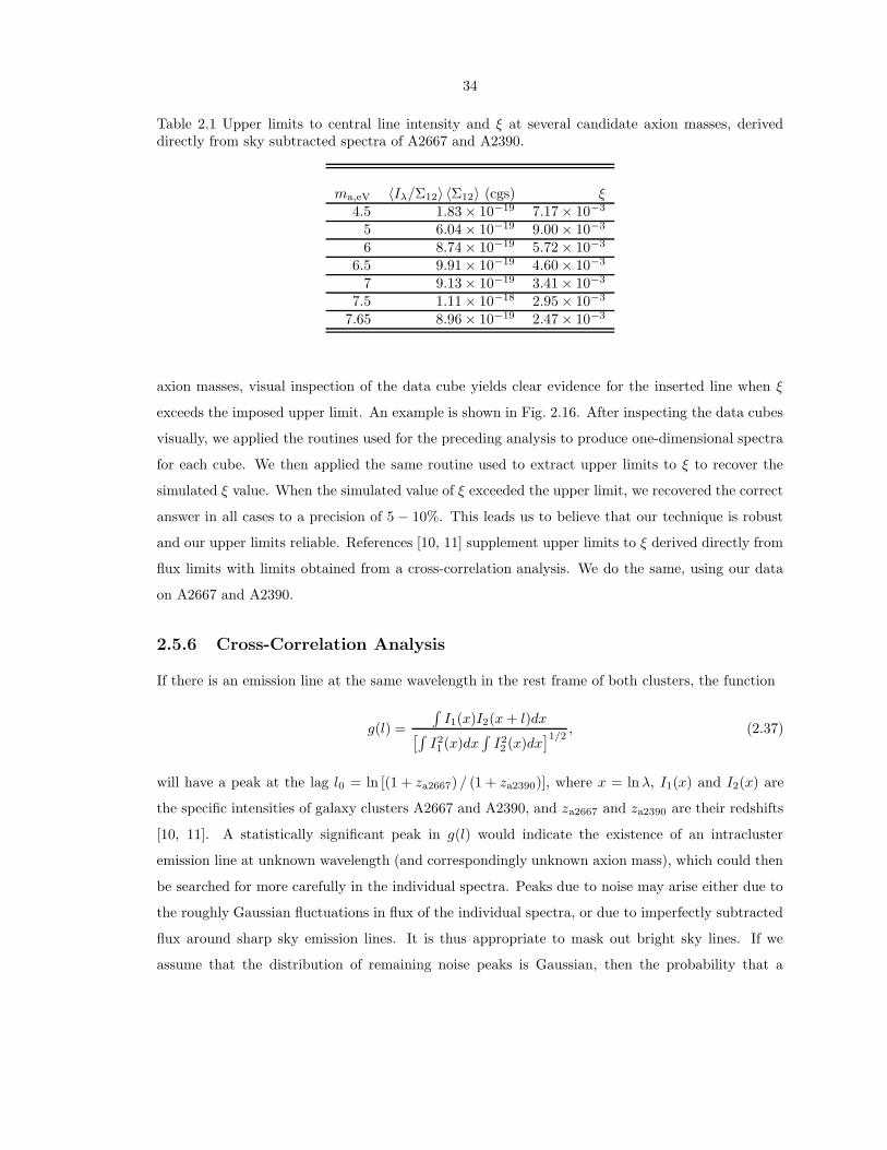
34

Table 2.1 Upper limits to central line intensity and ξ at several candidate axion masses, deriveddirectly from sky subtracted spectra of A2667 and A2390.

ma,eV 〈Iλ/Σ12〉 〈Σ12〉 (cgs) ξ4.5 1.83× 10−19 7.17× 10−3

5 6.04× 10−19 9.00× 10−3

6 8.74× 10−19 5.72× 10−3

6.5 9.91× 10−19 4.60× 10−3

7 9.13× 10−19 3.41× 10−3

7.5 1.11× 10−18 2.95× 10−3

7.65 8.96× 10−19 2.47× 10−3

axion masses, visual inspection of the data cube yields clear evidence for the inserted line when ξ

exceeds the imposed upper limit. An example is shown in Fig. 2.16. After inspecting the data cubes

visually, we applied the routines used for the preceding analysis to produce one-dimensional spectra

for each cube. We then applied the same routine used to extract upper limits to ξ to recover the

simulated ξ value. When the simulated value of ξ exceeded the upper limit, we recovered the correct

answer in all cases to a precision of 5− 10%. This leads us to believe that our technique is robust

and our upper limits reliable. References [10, 11] supplement upper limits to ξ derived directly from

flux limits with limits obtained from a cross-correlation analysis. We do the same, using our data

on A2667 and A2390.

2.5.6 Cross-Correlation Analysis

If there is an emission line at the same wavelength in the rest frame of both clusters, the function

g(l) =

∫

I1(x)I2(x+ l)dx[∫

I21 (x)dx

∫

I22 (x)dx

]1/2, (2.37)

will have a peak at the lag l0 = ln [(1 + za2667) / (1 + za2390)], where x = lnλ, I1(x) and I2(x) are

the specific intensities of galaxy clusters A2667 and A2390, and za2667 and za2390 are their redshifts

[10, 11]. A statistically significant peak in g(l) would indicate the existence of an intracluster

emission line at unknown wavelength (and correspondingly unknown axion mass), which could then

be searched for more carefully in the individual spectra. Peaks due to noise may arise either due to

the roughly Gaussian fluctuations in flux of the individual spectra, or due to imperfectly subtracted

flux around sharp sky emission lines. It is thus appropriate to mask out bright sky lines. If we

assume that the distribution of remaining noise peaks is Gaussian, then the probability that a

35

Figure 2.14 Comparison of existing limits to the two-photon coupling of a 4.5 eV−14 eV axion withthe projected sensitivity of our proposed observations of lensing cluster RDCS 1252 (z = 1.237).Flux limits and density profiles were assumed to be the same as those of A2667/A2390. The bestexisting upper limits to ξ in the higher mass window come from limits to the Diffuse ExtragalacticBackground Radiation (DEBRA), and were rescaled for consistency with today’s best-fit ΛCDMparameters and recent measurements [51, 64]. The limits reported in this and previous work, derivedusing optical spectroscopy of galaxy clusters, are shown for comparison [10, 11]. Regions inaccessibledue to night-sky emission lines are marked with narrow black arrows. The two solid horizontal linesindicate the predictions of the E/N = 2 hadronic and DFSZ axion models; the downward arrowsindicate that ξ is theoretically uncertain.

cross-correlation peak with height greater than or equal to s is due to noise is [10, 11]

P (≥ s) =

∫ ∞

s

e−x2/(4σ2g)dx√

πσg= 1− Erf

(

s

2σg

)

. (2.38)

Here, σg is the rms value of the antisymmetric component of g(l) and provides an estimate of

the correlation due to noise, since a Gaussian signal leads to a symmetric correlation function

[10, 142]. Equation (2.38) determines the statistical significance of peaks in g(l). Our analysis of

correlated spectra follows the treatment of Ref. [142]. We calculate g(l) using the sky subtracted

one-dimensional spectra of A2667 and A2390. With a cross-correlation technique, we are able to

perform a blind search for cluster rest-frame emission. We find no statistically significant (> 2σg)

cross-correlation peaks, as shown in Fig. 2.17.

We simulate our cross-correlation based search for an intracluster line in order to set alternative

upper limits to ξ [10, 11]. The limits reported in Ref. [11] were obtained using this technique. In our

simulation, we introduced ‘fake’ axion decay lines into both spectra and calculated the resulting g(l)

for a variety of values ma,eV, thus simulating the cross-correlation search for evidence of intracluster

emission. ξ was initially set to a value for which a very significant peak in g(l) appeared, and then

36

Figure 2.15 Limits on the combination ξ(

Ωah2)1/2

, derived directly from upper limits to the intr-acluster flux of A2667 and A2390. Our data exclude the shaded region. Data analysis proceeds asin the thermal case, but appropriate (more general) expressions for the intensity Iλ are used. Theseconstraints do not depend on the assumption that axions are produced thermally at early times.

ramped down until the peak at l0 ceased to be statistically significant; that is, until P (s) > 5%. At

that point, an upper limit on ξ was set. The cross-correlation peaks due to the axion line are well fit

by Gaussian curves throughout the ma,eV − ξ parameter space. Since the cross-correlation function

includes the contribution of flux away from the line center, rebinning was unnecessary.

To further distinguish between signal and noise peaks, we follow Ref. [10] in using the usual

criterion, |l− l0| ≤ σ, where σ is the width of the best Gaussian fit to g(l) around a cross-correlation

peak. We use this criterion in both the simulation and the cross-correlation search [10]. The resulting

limits to ξ at a series of candidate axion masses are shown in Table 2.2, and are on average a factor

of ∼ 1.5 less stringent than those derived directly from flux.

One aspect of the correlation analysis of Ref. [10] is troubling. Two noisy, imperfectly sky

subtracted spectra were correlated to search for a signal. The analysis of Ref. [10], however, uses

one real spectrum (containing noise and an imperfectly subtracted sky-background signal) with an

artificial axion line inserted, and a second, noiseless, template spectrum, containing only the artificial

axion line, but no imperfectly subtracted sky component. Thus, the method simulated in Ref. [10]

is not the same as the method used to actually search for evidence of an intracluster line, and by

artificially reducing the noise budget of the simulation, could lead to artificially stringent constraints.

The appropriate way to simulate the cross-correlation analysis is to correlate two real spectra with

artificial axion lines inserted, as we have done. Our data also place limits on the decay of other

37

Figure 2.16 The upper left panel of this figure shows a simulated 4255.2A slice of the A2667 IFUdata cube, with an axion-decay emission line inserted corresponding to ma,eV = 7.2 and ξ = 0.011.

The flux scale is in units of 10−18 erg s−1 cm−2 A−1

. This slice, which lies at the expected linecenter, shows evidence of the inserted axion line. The resulting ‘emission’ clearly traces the clustermass density profile. The lower left panel of this figure shows a simulated slice of the same datacube, but at 5267.2A, well away from the line center. As expected, no signature of axion emissionis present this far away in wavelength from the line center. The upper/lower right panels of thisfigure show 4255.2A/ 5267.2A slices, respectively, of the actual A2667 IFU data cube used for ouranalysis.

relics.

2.5.7 Sterile neutrinos

Our data might also be used to constrain the decay rate of other ∼ 5 eV relics, such as sterile

neutrinos [79–82]. Although the prevailing paradigm places the sterile-neutrino mass in the keV

range, some experimental data can be fit by introducing a hierarchy of sterile neutrinos, at least one

of which is in the 1− 10 eV range and could oscillate to produce photons in our observation window

[143, 144]. In our notation and in the me−,µ,τ ms limit (where ms is the sterile-neutrino mass),

the intensity of this signal is

⟨

Iλ,s

Σ12

⟩

= 2.4× 10−18Bm8

s,eV exp[

− (λr − λs)2c2/(

2λ2sσ

2)

]

σ1000(1 + zcl)4S2(zcl)cgs, (2.39)

where B is a model-dependent normalization factor, the oscillation is parameterized by a cumulative

mixing angle θ, and the additional power of mass arises from the late-time abundance of sterile

38

Figure 2.17 Cross-correlation function g(l) between sky subtracted spectra of clusters A2667 andA2390. No peaks with the desired statistical significance were seen, at the desired lag or elsewhere.A single cross-correlation peak is near the expected lag l = 0.00498 for an intracluster emission linecommon to A2667 and A2390. However, it is not statistically significant.

neutrinos [145]:

Ωsh2 = 0.3×m2

s,eV sin2 2θ. (2.40)

The flux limits in Table 2.1 impose the constraints B ≤ 8.03 × 10−5, 1.14 × 10−4, 9.41 ×10−5, 3.82×10−5, 2.28×10−5, 1.16×10−5, 8.12×10−6, and 5.61×10−6 for sterile-neutrino masses

of ms,eV = 4.50, 5.00, 5.50, 6.00, 6.50, 7.00, 7.50, and 7.65, respectively. In conventional models,

B = sin4 (2θ)/1011. The parameter B encodes the effects of both the early-universe production

and the decay of sterile neutrinos, which occurs at the rate Γs→ν+γ = 6.8× 10−38s−1m5s,eV sin2 2θ

[146–149]. By definition, B ≤ 10−11, and so optical data only constrain sterile neutrinos if some

novel mechanism increases the oscillation rate Γs→ν+γ by many orders of magnitude. The sharp

disparity between x-ray and optical constraints results from the Γ ∝ m5s scaling of the decay rate.

2.5.8 Ongoing Work

We have demonstrated the utility of applying integral field spectroscopy in concert with lensing data

to search for axions in z ' 0.2 galaxy clusters. Our technique could also be profitably applied to

higher redshift galaxy clusters. Although flux falls off as Iλ ∝ (1 + zcl)−4, the fact that we are

pushing to a higher mass range ma,eV = 24, 800A (1 + zcl) /λa increases the expected signal. Since

Iλ ∝ m7a,eV, the expected signal actually increases as Iλ ∝ (1 + zcl)

3. The most distant known

lensing cluster is RDCS 1252, at redshift z = 1.237 [150].

39

Table 2.2 Upper limits to ξ at several candidate axion masses, obtained from a simulation of thecross-correlation method, using spectra of A2667 and A2390.

ma,eV ξ4.5 2.73× 10−2

5 1.08× 10−2

6.0 9.35× 10−3

6.5 6.90× 10−3

7 4.44× 10−3

7.5 4.31× 10−3

7.65 2.16× 10−2

Using existing weak-lensing mass maps for this cluster [151] and creating our own strong-lensing

maps, we should be able to obtain a sky subtracted, spatially weighted spectrum of this cluster,

attaining flux levels similar to those we have obtained for A2667 and A2390. We will thus be able

to search for emission from decaying axions in the mass window 8 eV ≤ ma ≤ 14 eV. Assuming

identical cluster density profiles and flux limits, we estimate the range of ξ values accessible with

a telescope search for cluster axions in RDCS 1252. The tightest existing constraints to decaying

relic axions in this mass window come from limits to the diffuse extragalactic background radiation

(DEBRA) [51, 64]. As shown in Fig. 2.14, a VIMOS IFU search for axions in this mass window

would detect very weakly coupled axions, or alternatively, improve upper limits to ξ by two orders of

magnitude. Applying Eq. (2.16), we see that 8 eV− 14 eV axions would freeze out with abundance

0.12 ≤ Ωm ≤ 0.21. An axion detection in this mass window could thus account for most of the

dark matter; a telescope search in this mass window would provide a useful check of LSS constraints

to axion properties. Future discoveries of even higher redshift clusters could allow heavier axion

mass windows to be probed with cluster observations. We have obtained 18 hours of IFU data of

RDCS 1252 and the raw data have been reduced. At the moment, we are applying the existing

parameterized strong-lensing mass model of the cluster conduct a thermal new axion search.

2.6 Conclusions

The axion hypothesis offers attractive solutions to both the strong CP and dark-matter problems.

A series of null searches and astrophysical constraints has narrowed down the parameter space of

the axion to two mass windows, one between 10−5 eV and 10−3 eV, and the other between 3 eV

and 20 eV. Previous searches for optical emission from decaying axions in galaxy clusters have

constrained the two-photon coupling of the axion in the latter window. We have searched for axion-

decay light in the galaxy clusters A2667 and A2390, taking advantage of strong-lensing mass maps

of A2667/A2390 to free our analysis of dynamical assumptions. Use of the VIMOS IFU allowed an

40

increase in effective collecting area, thus increasing the sensitivity of our axion search. We observed

no evidence for emission from decaying axions in the mass window between 4.5 eV and 7.7 eV.

Conservatively, we improve on constraints to the two-photon coupling ξ of axions by a factor of

' 3, averaged over the entire mass range we explore. This work presents the first application of

IFU spectroscopy to constrain the nature of the dark matter and not just its spatial distribution.

To check that the stringency of our constraints is not an artifact of the rather complicated data-

reduction techniques inherent to IFU spectroscopy, we have simulated our technique by introducing

fake axion lines into our data cubes. Our analysis technique accurately recovers the value of ξ, and

the axion’s signature fades into the sky-background as ξ is ramped down below our reported upper

limits. Our simulations demonstrate the robustness of our technique, and our work highlights the

potential of IFU spectroscopy for more sensitive exploration of the axion mass window between 8 eV

and 14 eV.

Acknowledgments

The author thanks Giovanni Covone, Jean-Paul Kneib, Marc Kamionkowski, Andrew Blain, and

Eric Jullo for their contributions to the research described in this chapter. The author thanks Ted

Ressell and Matthew Bershady for helpful discussions. This research was supported by the Euro-

pean Community via the Marie Curie European Re-Integration Grant n.029159, the CNRS, DoE

DE-FG03-92-ER40701, NASA NNG05GF69G, the Gordon and Betty Moore Foundation, the Alfred

P. Sloan Foundation, and Research Corporation.

41

Chapter 3

Axion constraints in non-standard

thermal histories1

3.1 Introduction

The Peccei-Quinn (PQ) solution to the strong-CP problem yields the axion, a dark-matter candidate

[36, 47, 48]. If the axion mass ma ∼> 10−2 eV, axions will be produced thermally, with cosmological

abundance

Ωah2 =

ma

130 eV

(

10

g∗S,F

)

, (3.1)

where g∗S,F is the effective number of relativistic degrees of freedom when axions freeze out [50, 51,

86, 93]. Axions with masses in the ∼ eV range would contribute to the total density in roughly

equal proportion to baryons.

Axions in the ∼ eV mass range are relativistic when they decouple at TF = 30 − 50 MeV [93].

Free streaming then erases density perturbations, suppressing the matter power spectrum on scales

smaller than the axion free-streaming length [50, 152–154]. Light axions would also contribute to

the early integrated Sachs-Wolfe (ISW) effect [155]. Data from large-scale structure (LSS) surveys

and cosmic microwave-background (CMB) observations have been used to impose the constraint

ma ∼< 1 eV to light hadronic axions [6, 156, 157]. These arguments apply to any particle relativistic

at matter-radiation equality or cosmic microwave background (CMB) decoupling, thus imposing the

similar constraint∑

imν,i ∼< 1 eV to the sum of neutrino masses [16, 18, 154, 158–165].

These constraints rely on abundances computed assuming that radiation domination began earlier

than the chemical freeze-out of light relics. There is, however, no direct evidence for radiation

domination prior to big-bang nucleosynthesis (BBN) [166]. The transition to radiation domination

may be more gradual than typically assumed. In such a modified thermal history, two effects

may cause relic abundances to change. First, the Hubble expansion rate scales differently with

temperature T until radiation domination begins, leading to a different freeze-out temperature.

Second, entropy may be generated, suppressing relic abundances.

The universe could have reheated to a temperature as low as Trh ∼ 1 MeV, with standard

1The material in this chapter was adapted from Axion constraints in non-standard thermal histories, Daniel Grin,Tristan L. Smith, and Marc Kamionkowski; Phys. Rev. D 77, 085020 (2008). Reproduced here with permission,copyright (2008) by the American Physical Society. For the thesis, significant amounts of motivation and literaturereview were added in the introduction of this chapter. The discussion of the model-dependence of globular clusterlimits to axion properties is new. The discussions of pion equilibrium and axion production from nucleons wereextended as well.

42

radiation domination proceeding thereafter [26, 77, 78, 167–169]. This low-temperature reheating

(LTR) scenario may be modeled simply through the entropy-generating decay of a massive particle

φ into radiation, with fixed rate Γφ and initial value HI of the Hubble parameter. The scalar φ

may be the inflaton, oscillating as inflation ends and decaying into standard-model particles, or it

might be a secondary scalar, produced during preheating [170–174]. This decay softens the scaling

of temperature T with cosmological scale factor a, increasing the Hubble parameter H(T ) and

leading to earlier freeze-out for certain relics. Entropy generation then highly suppresses these relic

abundances.

Such low values of Trh are a far cry from the Planck and GUT (Grand Unified Theory) energy

scales of 1019 GeV and 1016 GeV, respectively. There are, however, several reasons to contemplate

such low-reheating temperatures. The first is epistemological. The simple fact is that we have very

little direct leverage on the thermal history of the universe before BBN. As long as neutrinos are

adequately thermalized and the expansion rate not too perturbed after T ∼< 10 MeV, the successful

predictions of BBN may be reproduced. Careful computations show that this constraint requires

Trh ≥ 4 MeV [78, 167], but this leaves many orders of magnitude to be explored. It thus behooves

us to at least consider the consequences of low reheating temperatures. It is also important not

to confuse the reheating temperature Trh (the temperature of the thermal plasma when radiation

domination begins) with Tmax, the maximum temperature ever achieved by the plasma after it

thermalizes [76, 169, 175, 176]. In a model driven by φ decays, Tmax may in fact be arbitrarily high

for a given value Trh. As a result, there is still acceptable parameter space for both electroweak

baryogenesis (if Trh > 100 GeV) as well as GUT baryogenesis [76, 169, 176] in models with LTR.

The second reason to seriously consider low values of Trh is that late-time entropy generation

can solve a classical flavor of cosmological problem, the overabundance of some ‘dangerous relic.’

For example, if gravitinos are thermally produced in the early universe, their relatively late decay

could change the expansion history during the sensitive BBN epoch, disassociate light nuclei after

they form, or inject energy afterwards and distort the CMB blackbody through the addition of a

chemical potential. These arguments impose the constraint Trh < 109 GeV [177]. In some areas

of supersymmetric parameter space, gravitinos may also be produced non-thermally through grav-

itational particle production. In that case, one obtains the considerably more stringent constraint

Trh ∼< 100 GeV [178].

The third reason to seriously consider low values of Trh relates to the second. Entropy generation

suppresses relic abundances and temperatures (for the case of thermal relics). The nature of dark

matter is as of yet unknown, though the list of candidates includes axions, weakly interacting

massive particles (WIMPs) such as neutralinos or gravitinos, heavy sterile neutrinos, and even

standard-model (SM) neutrinos. WIMPs are usually considered attractive dark matter candidates,

as a simple of order-magnitude estimate of the freeze-out abundance of a weakly-coupled massive

43

relic is generically close to the total dark matter density. This is the famous “WIMP miracle” [179].

Ongoing experiments, mainly the Large Hadron Collider (LHC), may detect supersymmetric

partner particles. They may turn out to have couplings and masses that yield exceedingly high

or low relic densities in the conventional thermal history, inconsistent with the usual “WIMP”

miracle. In that case, cosmologists might conclude that radiation domination began later than

usually assumed and was preceded by an epoch of entropy generation, or that the dark matter was

produced non-thermally [180]. It turns out that with an appropriate choice of reheating temperature

and direct couplings of the entropy-generating scalar to the SM, nearly any type of neutralino can

be made consistent with the total cosmological density of dark matter, Ωdh2 ' 0.12. In other words,

the usual cosmological constraints to WIMP properties are considerably relaxed if Trh is allowed to

take lower values [180].

Experiments like the LHC could thus drive the allowed values of Trh into a range much lower

than favored by conventional wisdom [181]. This could yield meaningful constraints on the very

early thermal history of the universe. It turns out that if a wino-like neutralino is detected at the

LHC, the demand that it constitute all/most of the dark matter would yield a fairly robust hint

of non-thermal dark matter production [180]. In this case of non-thermal dark matter production,

there is even a scenario called the ‘non-thermal WIMP miracle’ [182]. Here, the number density

of WIMPs approaches an attractor solution which balances the competing WIMP source of φ de-

cays/annihilations with WIMP annihilation. In fact, Ωdh2 ∼ 0.12 is obtained rather generically,

contradicting the usual heuristic claim that the standard thermal history provides a more natural

framework for obtaining the observed dark matter abundance.

Similarly, experiments like the Axion Dark Matter eXperiment (ADMX) [27] or CERN (Conseil

Europeen pour la Recherche Nucleaire) Axion Solar Telescope (CAST) [28] may discover an axion

with mass ma < 10−2 eV, which would be coherently produced in the early universe [111]. If ma is

sufficiently low, the relic density of such axions as computed by Eq. (2.19) may drastically exceed

Ωd. If the axion is the dark matter, an era of entropy generation may be invoked to adequately

dilute these ‘misalignment’ axions. If, on the other hand, WIMPs constitute the bulk of the dark

matter, an era of entropy generation may also be invoked to dilute non-thermal axions to negligible

densities. In other words the usual cosmological constraint (ma ∼> 10−5 eV) to the properties of

coherently-produced axions may be considerably relaxed if Trh is allowed to take lower values. More

precisely, in the LTR scenario, coherently produced axions (with fa finf) have abundance [76, 183]

Ωah2 ∼ 2× 10−7

( ma

10−5 eV

)−1.52(

Trh

MeV

)1.96

. (3.2)

If we saturate the BBN constraint on reheating by choosing Trh = 4 MeV, the constraint Ωah2 < 0.12

imposes the less stringent constraint that ma ∼> 10−8 eV, giving experiments searching for coherently

44

produced axions a few additional orders of magnitude in mass to search.

It is also possible (though depressing to consider) that the LHC, ADMX, CAST, CDMS (Cold

Dark Matter Search) [32], and the bevy of other current and future experiments designed to seek

super-symmetry or directly detect WIMP/axions will all fail to detect new particles. Other more

mundane dark matter candidates may be worth a second look in this case, specifically SM neutrinos.

It turns out that ∼ keV (warm) SM neutrino dark matter can be made compatible with cosmological

constraints if Trh ∼ MeV [76, 77]. Heavy, right-handed neutrinos are sometimes invoked to explain

SM neutrino masses using the ‘seesaw’ mechanism [143, 144, 184]. They would mix weakly with

SM neutrinos and be non-thermally produced in the early universe [80–82, 145, 185, 186]. Sterile

neutrinos in the ∼ keV range are a frequently discussed dark matter candidate [79, 148, 187–194],

and cosmological constraints on their mixing angles are considerably relaxed in the LTR scenario

[195–197].

The fourth reason to consider the LTR scenario is that it is actually quite natural [198]. Light

moduli fields abound in many realizations of string theory and M-theory, and their mass may very

well lie in the range 10 TeV ∼< mφ ∼< 100 TeV. These fields are gravitationally coupled, and thus

decay with width [198]

Γ ∼m3

φ

m2pl

, (3.3)

where mpl is the Planck mass. These scalars may dominate the energy budget of the universe

during the epoch following inflation and until radiation-domination. The reheating temperature

Trh is then obtained by setting Γ ∼ H(Trh) (We use the standard radiation dominated expression

H (Trh) ∼ T 2/mpl, as it should be valid at the transition temperature between the entropy-generating

and radiation-dominated epochs). The resulting reheating temperature is [182]

Trh ∼ 10 MeV( mφ

100 TeV

)3/2

, (3.4)

and so Trh ∼ 10 MeV is not as far-fetched as it may naively seem.

Kination models offer another alternative to the standard thermal history, invoking a period of

scalar-field kinetic-energy dominance [199], but no entropy production. During kination, ρφ ∝ a−6,

where a is the cosmological scale factor, and H (T ) ∝ T 3. This behavior is rather generic in

quintessential inflation models [200–202], where one scalar field is responsible for both primordial

inflation and ‘dark energy today.’ In these models, reheating typically occurs through gravitational

particle production. As the scalar rolls down its potential, it becomes kinetic-energy dominated, and

so ρφ ∝ a−6 damps away. Deep into matter domination, the small residual potential energy density

of φ becomes important again, relative to the matter density ρmatter. In quintessential inflation, this

is responsible for the late-time acceleration of a.

Kination has many appealing features, however, that depend in no way on its specific embedding

45

in a more complete model, but require only an era with ρ ∝ a−6 [203, 204]. The slightly larger Hubble

parameter during kination makes it easier to satisfy the out-of-equilibrium condition required for

successful baryogenesis [203]. It has been shown that successful electroweak baryogenesis is possible

in cosmologies with a kination epoch [203, 205, 206]. The lack of entropy generation in kination

models also means that a successfully generated baryon asymmetry is not diluted away.

Earlier freeze-out of WIMPs and other heavy relics leads to higher relic densities. As in the

case of low-temperature reheating, this means that cosmological constraints to WIMP properties

are relaxed [207, 208], and that collider experiments can be used to put meaningful constraints on

the duration of the kination epoch. One exciting possibility is that for 4 sensible benchmark models

in minimal supergravity, the combination of the LHC and ILC (International Linear Collider) will be

sufficient to discover a kination epoch preceding BBN (assuming of course, that the supersymmetric

particle discovered at colliders is also the dark matter) [29].

Past work has shown that cosmological constraints to neutrinos, weakly interacting massive

particles, and non-thermally produced axions are relaxed in the LTR [76, 77, 195] and kination

scenarios. Non-thermally produced axions (ma ∼< 10−2 eV) would be produced through coherent

oscillations of the PQ pseudoscalar [50–52], as discussed in Sec. 2.2. In this chapter, we obtain new

constraints to thermally-produced hadronic axions in the kination and LTR scenarios. Thermal

axions freeze out while relativistic, and so without entropy generation, their abundances change

more modestly than in the LTR case. While kination modestly loosens limits, LTR dramatically

changes the cosmologically allowed range of axion masses.

We begin by reviewing these modified thermal histories and calculating axion relic abundances.

We then generalize cosmological constraints to axions, allowing for low-temperature reheating and

kination. For reheating temperatures Trh ∼< 35 MeV, LSS/CMB limits to the axion mass are lifted;

constraints are also relaxed for higher Trh. Constraints from the total matter density are also

relaxed, but not completely lifted. For Trh ' 10 MeV, the new constraint is ma ∼< 1.4 keV, while

for Trh ' 35 MeV, we find that ma ∼< 43 eV. If Trh ∼> 170 MeV, standard results are recovered.

We thus see that for sufficiently low Trh, thermal axions are a warm dark matter candidate. After

estimating the ability of future large-scale-structure surveys to further constrain axion masses for a

variety of reheating temperatures, we derive modestly relaxed constraints to axions in the kination

scenario. We conclude by considering future possible constraints to the relativistic energy density

of axions in a low-temperature reheating model.

46

3.2 Two non-standard thermal histories: Low-temperature

reheating and kination

We now review the low-temperature reheating (LTR) scenario. We consider the coupled evolution

of unstable massive particles φ, which drive reheating, and radiation R, both in kinetic equilibrium.

The relevant distribution functions obey a Boltzmann equation with a decay term, and may be

integrated to yield [76, 77, 175]:

1

a3

d(

ρφa3)

dt= −Γφρφ,

1

a4

d(

ρRa4)

dt= Γφρφ, (3.5)

where ρφ and ρR denote the energy densities in the scalar field and radiation, respectively, Γφ is the

decay rate of the scalar to radiation, and a is the cosmological scale factor. The evolution of the

scale factor is given by the Friedmann equation, which is H2 = [8π/(3M2pl)] (ρφ + ρR) well before

matter or vacuum-energy domination. The reheating temperature Trh is defined by [50, 76, 175]

Γφ ≡√

4π3g∗,rh45

T 2rh

Mpl, (3.6)

where Mpl is the Planck mass and g∗,rh is the effective number of relativistic degrees of freedom

when T = Trh. In our calculation of the expansion history in LTR, we use g∗ calculated using the

methods of Refs. [50, 209], as tabulated for use in the DarkSUSY package [210]. We neglect the

axionic contribution to g∗ for simplicity and assume 3 massless neutrinos. The resulting ∼ 10%

error in g∗ leads to a comparable fractional error in the resulting axion relic abundance, and is thus

negligible at our desired level of accuracy.

We use dimensionless comoving densities [76, 175]:

Φ ≡ ρφT−1rh T−3

0 a3, R ≡ ρRa4T−4

0 , (3.7)

where T0 is the temperature today. At the beginning of reheating, φ dominates the energy density

and radiation is negligible. Thus, as initial conditions, we use ρR = 0 and ρφ = [3/ (8π)]M2plH

2I ,

where HI is the initial value of the Hubble parameter. The two physical free parameters in this

model are Trh and HI. The temperature is related to the radiation energy density by [50]

T =

[

30

π2g∗(T )

]1/4

ρ1/4R . (3.8)

We numerically integrate Eqs. (3.5) to obtain the dependence of T on a, and the results are shown

in Fig. 3.1. As the scalar begins to decay, the temperature rises sharply to a maximum at am =

(8/3)2/5

aI, where aI is the initial value of the scale factor, and then falls as T ∝ a−3/8. This shallow

47

scaling of temperature with scale factor results from the continual dumping of scalar-field energy

into radiation, and yields an unusually steep dependence of scale factor on temperature. As shown

in Figs. 3.1 and 3.2, when the comoving radiation energy density R overtakes Φ near T ∼ Trh, the

epoch of radiation domination begins, with the usual T ∝ a−1 scaling.

Well before reheating concludes, Φ is constant and ρR ρφ. If am a < a (Trh), an approximate

solution of Eqs. (3.5) for T (a) is then [76, 175]

T ' Tmax

(

a

am

)−3/8 [g∗ (Tm)

g∗ (T )

]1/4

Tmax = 4.2 GeV

[

10g∗,rhg2∗ (Tm)

]1/8

H1/4I,eVT

1/2rh,MeV, (3.9)

where g∗,rh = g∗ (Trh) and Tmax is the maximum temperature obtained (see Fig. 3.1). Here Trh,MeV

and HI,eV are the reheating temperature and initial value of the Hubble parameter, in units of MeV

and eV, respectively.

During reheating, the Hubble parameter is given by [76, 77]

H '[

5π3g2∗ (T )

9g∗,rh

]1/2(T

Trh

)2T 2

Mpl. (3.10)

At a given temperature, the universe thus expands faster during reheating than it would during

radiation domination, and the equilibrium condition Γ ≡ n 〈σv〉 ∼> H is harder to establish and

maintain. Relics with freeze-out temperature TF ≥ Tmax will thus have highly suppressed abundances

because they never come into chemical equilibrium. Relics with Trh ∼< TF ∼< Tmax come into chemical

equilibrium, but then freeze out before reheating completes. Their abundances are then reduced by

entropy production during reheating. In either case, species with TF ∼> Trh have highly suppressed

relic abundances.

Less radical changes to abundances follow in kination scenarios. During epochs dominated by

the kinetic energy of a scalar field, the energy density ρ scales according to ρ ∝ a−6 [199]. Thus

H (T ) ∝ T 3 or H ' Hrad (T ) (T/Tkin), where Hrad (T ) is the standard radiation-dominated H (T )

and Tkin denotes the transition temperature from kination to radiation domination. Kination yields

relic freeze-out temperatures somewhere between the standard and LTR values. There is, however,

no entropy generation during kination, leading to a less dramatic change in relic abundances. Note

that these conclusions are rather general, as we have not relied on any detailed properties of the

kination model, but only on the scaling H (T ) ∝ T 3 [166].

48

Figure 3.1 This plot shows the evolution of temperature with scale factor in a low-temperaturereheating (LTR) scenario with Trh = 20 MeV and 3 different initial values for the Hubble parameterHI. After a rapid rise due to φ decay, T ∝ a−3/8 until T ∼ Trh, after which radiation dominationbegins, and T ∝ a−1. The small bump near T ' 200 MeV results from a jump in g∗ near the QCDphase transition.

3.3 Axion production in non-standard thermal histories

Axions with ma ∼> 10−2 eV are thermally produced in the standard radiation-dominated cosmology.

We now show that in LTR models, these axions have suppressed abundances. We consider standard

hadronic axions, which do not couple to standard-model leptons but do couple to pions and photons

through higher order terms [56, 57]. We do not consider flaton models, or other scenarios in which

PQ symmetry breaking is related to supersymmetry breaking [211–215]. For temperatures T ∼<

150 MeV, the dominant channels for axion production are π+ + π− → a+ π0, π+ + π0 → π+ + a,

and π− + π0 → a + π− [93]. Axion scattering rates are suppressed relative to particle-number-

changing interactions by factors of T 2/f2PQ and thus decouple very early. Thus, axions stay in

kinetic equilibrium because of π + π ↔ a+ π, and kinetically decouple when they chemically freeze

out.

Nucleonic channels are negligible at these temperatures [93], as we verify below. If pions are in

chemical equilibrium and Bose enhancement can be neglected, the axion production rate is obtained

49

Figure 3.2 The top panel shows the Hubble parameter as a function of temperature in an LTRcosmology with Trh = 20 MeV and HI = 1 MeV. Initially H ∝ T 4g∗ (T ), but at temperaturescooler than T ∼ Trh, H ∝ T 2

√

g∗ (T ).The second panel shows the comoving radiation energydensity R = ρRT

−40 a4 and scalar energy density Φ = ρφT

−30 T−1

rh a3 as a function of temperature. AtT ∼ Trh, R flattens out to a constant and Φ drops off to zero, indicating the conclusion of reheating.

from the Lagrangian in Eq. (2.15) to be [6, 50, 93, 216]

Γ =3ζ(3)T 5C2

aπ

1024π7f2a f

2π

∫

dx1dx2x2

1x22

y1y2f(y1)f(y2)

∫ 1

−1

dµ

[

s−m2π

]3 [5s− 2m2

π

]

s2T 4,

Caπ =1− r

3 (1 + r), s = 2

[

m2π + T 2 (y1y2 − x1x2µ)

]

, (3.11)

where xi = pi/T is the dimensionless pion momentum, yi =√

x2i +m2

π/T2 is the dimensionless

pion energy, f (yi) = 1/ [exp (yi)− 1] is the pion distribution function, Caπ is the dimensionless

axion-pion coupling constant, and ζ(x) is the Riemann ζ-function. The PQ energy scale is fa. The

neutral pion mass is mπ ' 135 MeV [91]. The PQ scale can be expressed in terms of the axion mass

[87]:

fa '√r

1 + r

fπmπ

ma. (3.12)

Here r ≡ mu/md ∼ 0.56 is the up/down quark mass ratio and fπ ' 93 MeV is the pion decay

constant [50, 91].

Evaluating Eq. (3.11) for Γ and numerically solving Eq. (3.5) for H (T ), we estimate the axion

50

freeze-out temperature using the condition Γ (TF) ∼ H (TF). As the reheating temperature is low-

ered, axions freeze out at higher temperatures due to the higher value of H , as shown in Fig. 3.3.

As the reheating temperature is increased, the T ∝ a−3/8 epoch becomes increasingly irrelevant,

and the freeze-out temperature of the axion asymptotes to its standard radiation-dominated value.

Examining Eq. (3.11), we see that Γ ∝ f−2a ∝ m2

a, so higher-mass axions keep up with the Hubble

expansion for longer and generally decouple at lower temperatures. Thus, for higher ma, a more

radical change to the thermal history (even lower Trh), is needed to drive TF to a fixed higher value.

Figure 3.3 Freeze-out temperature of the reactions π+ + π− ↔ π0 + a, π+ + π0 ↔ π+ + a, andπ− + π0 ↔ π− + a, shown as a function of the reheating temperature Trh, for 4 different axionmasses. More massive axions are coupled more strongly, leading to later freeze-out than for lighteraxions.

As axions are spin-0 relativistic bosons, their number density at freeze-out is na (Tf) = ζ(3)T 3F/π

2.

If we assume that axion production ceases at freeze-out, the density of axions at any subsequent time

is just na (Tf) [aF/a0]3, where aF is the value of the cosmological scale factor at axion freeze-out.

The reheating time scale, trh ' 1/Γ, is much shorter than the Hubble time for T ∼< Trh, and so it is a

good approximation to treat the break between the T ∝ a−3/8 and T ∝ a−1 epochs as instantaneous

at T = Trh. Doing so, we apply Eq. (3.9) prior to the completion of reheating and a ∝ T−1g−1/3∗S (T )

afterwards, to obtain

Ωah2 =

ma,eV

130

(

10

g∗S,F

)

γ (Trh/TF) ,

51

γ(β) ∼

β5(

g∗,rh

g∗,F

)2 ( g∗S,F

g∗S,rh

)

if β 1,

1 if β 1,(3.13)

where ma is the axion mass in units of eV.

Low reheating temperatures drive up the freeze-out temperature. When Trh ∼< TF, the present

mass density in axions is severely suppressed, because of the sharper dependence of the scale factor

a on T during reheating. This is a result of entropy generation. Using the numerical solution for

a (T ) from Sec. 3.2, we obtain Ωa, accounting for the smooth transition between the T ∝ a−3/8 and

T ∝ a−1 regimes. In Fig. 3.4, we show Ωa normalized by its standard value, Ω0a, as a function of

Trh. At reheat temperatures just a factor of a few below the usual axion freeze-out temperature for

a given axion mass, the axion abundance is suppressed by a factor of 10−4 − 10−3. For Trh TF,

the axion abundance asymptotes towards its standard value. We see that the constraints on axion

decay from Chapter 2.5.3 then imply a very strict limit Trh 10 MeV if E/N = 2 is fixed there,

and uncertainties in mu/md are ignored.

In the case of kination, axion freeze-out temperatures are still raised, but there is no additional

entropy production. Axion abundances are given by Eq. (3.1), but with the higher g∗S,F values

appropriate at higher values of TF.

For the LTR case, our results do not depend on the initial value HI of the Hubble parameter.

As seen in Fig. 3.1, changes to HI determine the moment of the fast rise to Tmax, but have little

influence on the expansion history for T < Tmax. For convenience, we choose HI = 1 MeV for our

calculations, corresponding to Tmax ' 20 GeV.

Our calculation is valid only if axions are produced in equilibrium by thermal pions. We check

that pions are in chemical equilibrium using the chiral Lagrangian density term for pion-photon

interactions, which scales as [217]

Lππγγ ∼απ0π0FµνF

µν

f2π

. (3.14)

We use standard expressions for the number density of pions in the non-relativistic regime, and

estimate the cross-section for the ππ ↔ γγ reaction accurate to order-of-magnitude level assuming

that the photon momentum k ∼ T . Using the usual Γ (TF) ∼ H (TF) criterion, we estimate that

pions stay in equilibrium from the QCD phase transition until long after nucleosynthesis (down to

T ∼ keV, yielding exponentially suppressed abundances today), and so we may use equilibrium

expressions for the number density of pions.

For axion freeze-out to occur during the era where pions have condensed out of the quark-gluon

plasma, we must have Trh ∼> 10 MeV. Outside this range, our assumptions break down. For

sufficiently low values of ma and Trh, pionic cross sections lead to TF ∼> 200 MeV, earlier than the

quark-hadron phase transition. The absence of hadrons then necessitates the use of quark-axion

52

production cross sections.

Furthermore, for Trh ∼< 10 MeV, pions will decay before they can come into equilibrium. In both

cases, axion abundances are suppressed relative to our calculation. For axion masses saturating our

upper limits and Trh ∼> 10 MeV, we have checked that we are well within the equilibrium regime.

We restrict ourselves to this range, noting that for Trh ∼< 10 MeV, more suppressed abundances will

lead to an even more dramatic relaxation to cosmological axion limits. Coherent oscillations of the

axion field produce a condensate that behaves as cold dark matter [76], but the resulting additional

abundance is negligible for ma ∼> 10−2 eV at all values of Trh under consideration here [76].

It is instructive to verify that production off the ample thermal bath of protons and neutrons for

T ∼< ΛQCD is indeed negligible in our regime of interest. In low-energy chiral perturbation theory,

the axion-nucleon interaction Lagrangian density is [93]

LaN =∂µA

fa

(

CaNnγµγ5n+ Cappγ

µγ5p)

, (3.15)

where A is the axion field, CaN is the axion-neutron coupling constant, and Cap is the axion-proton

coupling constant. Both coefficients are of order unity. The lowest-order axion-nucleon reactions

are NN → NN a and Nπ → N a. Using an equilibrium value for the total nucleon density (adequate

because the baryon asymmetry is not very relevant until T ∼ 22 MeV when nucleons freeze out

[50]), we obtain the following expression for the ratio of the relevant chemical reaction rate to the

Hubble expansion

Γ

H=

611m2a,eV

√

mN

T e−mNT if T < Trh,

6.11× 10−4m2a,eV

(

Trh

MeV

)2√

m5N

T 5 e−mN

T if T > Trh.(3.16)

Numerically, we find that for the range of ma and Trh considered in this paper, the freeze-out

temperature TF of the nucleon-axion chemical reactions lies in the range 100 MeV ∼< TF ∼< 200 MeV.

Thus, our assumption that the pionic reactions dominate over the nucleonic ones is solid.

3.4 Constraints to axions

Most constraints to the axion mass are obtained from its two-photon interaction. This interaction

is parameterized by a coupling constant gaγγ, given by [4, 10, 11, 28, 42, 50, 51, 53, 74, 75, 218, 219]

ga→γγ = − α

2πfa

3ξ

4, (3.17)

53

Figure 3.4 Axion abundance Ωa normalized by its standard value Ω0a, shown as a function of the

reheating temperature Trh. Curves are shown for 4 different axion masses. More massive axionsfreeze out later. As a result, their density is less diluted by entropy production during the reheatingepoch, and so they have higher relic densities.

where ξ is a model-dependent parameter and α is the fine-structure constant. The tightest constraint

to ga→γγ ,

gaγγ ∼< 0.6× 10−10 GeV−1, (3.18)

comes from the helium burning lifetime of stars in star clusters [4, 220]. The parameter ξ is given

by [4, 53, 89, 218]

ξ =4

3

[

E

N− 2

3

(4 + r)

(1 + r)

]

. (3.19)

Here E and N are weighted sums of the electric and PQ charges of fermions that couple to axions,

as discussed in Chapter 2. In existing axion models, 0 ≤ E/N < 8/3 [86, 89], while r is poorly

constrained and lies in the range [89, 221–223]:

0.2 ≤ r ≤ 0.8. (3.20)

As a result, for any axion model in the range 1.93 ∼< E/N < 2.39, there are experimentally

allowed r values for which ga→γγ vanishes (see Eq. 3.19), and so constraints to axions from star

clusters, helioscope, RF cavity, and telescope searches may all be lifted [86, 89]. These constraints

are discussed in detail in Chapter 2. Such a cancellation is fine tuned, but even for other values of

E/N , constraints to the axion mass are loosened. In Ref. [89], the authors show that the null results

54

Figure 3.5 Upper limit to the axion mass from the evolution of horizontal branch (HB) stars inglobular clusters. Limits are shown as a function of the up/down quark mass ratio r = mu/md,for four different axion models, parameterized by the value of E/N . The region above the line isexcluded, while below the line is allowed. Limits to ga→γγ are taken from Refs. [4, 5] and generalizedto varying r and E/N .

of the ADMX experiment are actually still consistent with all the dark matter in the galactic halo

consisting of E/N = 2 axions. To further illustrate our point about the lifting of axion constraints

based on ga→γγ , we show the constraint from globular cluster stellar lifetimes [Eq. (3.18)] generalized

to the case of varying r and E/N ; to our knowledge, such an illustration does not yet exist in the

literature. We see that the globular cluster limit may be significantly relaxed when the full model

dependence of ga→γγ is considered.

In contrast, the hadronic couplings do not vanish for any experimentally allowed r values [86].

Axion searches based on these couplings are underway, and have already placed new upper limits to

the axion mass in the keV range [124] (and references therein). These couplings also determine the

cosmological abundance of axions, and so useful constraints may be obtained from cosmology.

Although the hadronic coupling determines the relic abundance of axions, ξ will determine the

lifetime of the axion, which may have implications for cosmological constraints. For the high axion

masses allowed by our new constraints and certain values of r and E/N , the decay a→ γγ may no

longer be negligible on cosmological time scales. Such an axion would be completely unconstrained

by limits to Ωah2 from the total matter density or the hot dark matter mass fraction. In the following

calculation, we neglect axion decay. Consistent with a vanishing two-photon coupling for E/N = 2,

we use the value r = 0.50. We have verified that our results for Ωah2 vary by only 5% for variations

55

in r of about 20%, as the dependence of the axion production rate and TF on r is weak (see Eq. 3.11)

compared with the dependence on the e−mπ/T Boltzmann factor.

3.4.1 Constraints to the axion mass from Ωmh2

In the standard cosmology, a conservative constraint is obtained by requiring that axions not exceed

the total matter density of Ωmh2 ' 0.135 [16], yielding the limit ma ∼< 22 eV, using a concordance

value for the dimensionless Hubble parameter h = 0.73. In LTR scenarios, axion abundances are

highly suppressed, as shown in Eq. (3.13) and Fig. 3.4. Mass constraints to thermal axions from

cosmology are thus considerably relaxed.

To obtain abundances in the LTR scenario, we apply the numerical freeze-out and abundance

calculation of Section 3.3. Axion mass limits resulting from the requirement that axions not exceed

the total dark matter density are shown by the dot-dashed hashed region in Fig. 3.6. If Trh ∼< 40 MeV,

constraints are considerably relaxed. For example, if Trh ' 10 MeV, the axion mass constraint is

ma ≤ 1.4 keV. When Trh ∼> 95 MeV, we obtain ma ∼< 22 eV, equal to the standard radiation-

dominated result. As already discussed, abundances are only slightly changed in the case of kination,

so Ωah2 imposes the constraint ma ∼< 26 eV if Tkin ' 10 MeV.

3.4.2 Constraints to the axion mass from CMB/LSS data

Axions will free stream at early times, decreasing the matter power spectrum on length scales smaller

than the comoving free-streaming scale, evaluated at matter-radiation equality. For sufficiently

low masses, axions will also contribute to an enhanced early ISW effect [155] in the CMB. This

suppression is given by ∆P/P ' −8Ωa/Ωm if Ωa Ωm [6, 156, 224] (and references therein). The

matter power spectrum thus imposes a constraint to Ωah2.

First we review the constraints imposed by these effects in a standard thermal history. In

this case, both Ωah2 and the free-streaming scale, λfs, depend only on ma in a hadronic axion

model. Using Sloan Digital Sky Survey (SDSS) measurements of the galaxy power spectrum [19] and

Wilkinson Microwave Anisotropy Probe (WMAP) [15] 1st-year measurements of the CMB angular

power spectrum, Refs. [6, 156, 224] derived limits of ma ∼< 1 eV. Axions in the mass range of interest

(ma ∼> 1 eV) are non-relativistic at photon-baryon decoupling, and so this constraint essentially

comes from measurements of the galaxy power spectrum [158]. As a result, we do not expect that

an analysis including more recent WMAP results would make a substantial difference in the allowed

axion parameter space. In order to lift this constraint, the relationship between ma and Ωah2 or

λfs must be changed. More recent results obtained using the WMAP 5th and 7th-year data releases,

assuming the standard thermal history [128, 130], confirm this intuition, and the authors even note

that the dominant contribution to the axion mass constraint comes from the LSS data.

56

If TF is allowed to vary freely, the constraints may be relaxed. In particular, using Eq. (3.1) we

can see that increasing g∗S,F (and thus TF) will decrease Ωah2. Furthermore, if the free-streaming

length of the axion is less than the smallest length scale on which the linear power-spectrum may be

reliably measured (λmin ' 40 h−1 Mpc), its effect on the matter power spectrum is not observable

[6, 156, 224]. The comoving free-streaming length scale at matter-radiation equality2 [50],

λfs '196 Mpc

ma,eV

(

Ta

Tν

)

1 + ln

[

0.45ma,eV

(

Tν

Ta

)]

, (3.21)

is set by the ratio between the axion and neutrino temperatures,

Ta

Tν≈ (10.75/g∗S,F)1/3, (3.22)

so that if g∗S,F ∼> 87 (i.e., if axions freeze out considerably before neutrinos), the constraint to axion

masses is lifted [6].

Figure 3.6 Upper limits to the hadronic axion mass from cosmology, allowing the possibility of alow-temperature-reheating scenario. The orange region shows the region excluded by the constraintΩah

2 < 0.135 as a function of reheating temperature Trh. The red region shows the additional partof axion parameter space excluded by WMAP1/SDSS data. At low reheating temperatures, upperlimits to the axion mass are loosened. For Trh ∼> 170 MeV, the usual constraints are recovered.

In the case of a modified thermal history, the relationship between TF and ma acquires depen-

dence on an additional parameter (Trh, in the case of LTR, or Tkin, in the case of kination) thus

allowing us to loosen the constraints. At a series of values of g∗S,F, Refs. [6, 156, 224] determine the

2This differs from the expression in Refs. [154, 224] because we assume, as is the case in our parameter region ofinterest, that m > Teq, the temperature at matter-radiation equality. In Ref. [154], m < Teq is assumed.

57

maximum values of Ωah2 consistent with WMAP measurements of CMB power spectra and SDSS

measurements of the galaxy power spectrum, as shown in Fig. 3.7.

Figure 3.7 Minimum allowed g∗S,F for a variety of Ωah2, taken from Ref. [6], reproduced here

with permission. The dark area shows the 1σ allowed region, while the region covered by thelight and dark areas shows the 2σ allowed region. Taken together with the hadronic freeze-outrelationship in a standard radiation dominated universe, these constraints impose the axionic massbound ma ∼< 1.05 eV.

We begin by mapping those contours (which do not include constraints from the Lyman-α forest),

shown in Fig. 3.7), into the(

Ωah2, λfs

)

plane. For a fixed ma or Ωa, λfs scales monotonically with

g∗S,F, and thus serves as a proxy for g∗S,F.

In the domain 10 MeV ≤ Trh ≤ 250 MeV and 0.01 eV ∼< ma ∼< 10 keV, we calculate Ωa (Trh,ma)h2

for hadronic axions in LTR, using the full numerical solution described in Sec. 3.3. We also calculate

λfs (Trh,ma). Since axions freeze out while relativistic, their energy will redshift as E ∝ a−1. They

will have temperature Ta = TFaF/a. Meanwhile, the temperature of the coupled radiation redshifts

as T ∝ a−3/8 until radiation domination begins. Thus entropy generation modifies the relationship

between the axion and neutrino temperatures to

Ta

Tν'(

11

4

)1/3(Trh

TF

)5/3(

g2∗,rhg∗S,0

g2∗,Fg∗S,rh

)1/3

, (3.23)

if TF > Trh. To obtain all of our constraints we use the more precise scaling accounting for the

smooth transition between the T ∝ a−3/8 and T ∝ a−1 regimes. The dominant change to the free-

streaming length comes from the modified axion temperature, while the modified expansion rate

itself induces negligible fractional changes of order TNR/Trh, where TNR is the cosmic temperature

at which the axion goes non-relativistic.

For each pair (Trh,ma), we calculate Ωah2 and λfs to trace out the region forbidden with 95%

58

confidence. When Ωa (Trh,ma)h2 > 0.014, outside the domain of Ref. [224], we extrapolate, as-

suming that the 95% contour asymptotes to a line of constant axion free-streaming wavelength

λfs = 40 h−1 Mpc. Such a trend is noted in Ref. [224], and at the maximum value of Ωah2 of the

contour obtained from Ref. [6], the maximum allowed free-streaming length is consistent with our

assumed asymptote.

We obtain the upper limit to the axion mass as a function of Trh, shown in Fig. 3.6. Existing

LSS/CMB constraints are severely relaxed in the LTR scenario, and lifted completely for Trh ∼<

35 MeV. For Trh ∼< 35 MeV, λfs < 40 h−1 Mpc forma ∼> 1 eV, and so the axion mass is cosmologically

constrained only by the condition Ωah2 ∼< 0.135. It will still be subject to phase-space constraints

if it is to compose all the dark matter in galactic halos [105–107]. Applying Eq. 2.27, we see

that the galactic phase space constraint with xa = Ωa/Ωm = ΩD/Ωm is ma > 22 eV. Thus, for

Trh < 35 MeV, there is an open axion mass window (which actually depends on Trh, but we give

rough numbers for simplicity) for 20 eV ∼< ma ∼< 700 eV, provided other astrophysical constraints

may be ignored. In future work, it will be interesting to apply the usual constraints to warm dark

matter (WDM) candidates to further constrain such a possibility.

At high reheating temperatures, the constraint from LSS/CMB data (Ωah2 ∼< 0.006) supercedes

the constraint Ωah2 ∼< Ωmh

2. The narrow allowed region between the LSS/CMB and total matter

density constraints in Fig. 3.6 (45 MeV ∼< Trh ∼< 55 MeV) may be simply understood. Axions in

this narrow window are cold and massive enough to evade large-scale structure constraints (i.e.,

λfs < λmin), and dilute enough to evade constraints from the total matter density. We note that the

CMB/LSS limits asymptote to their standard value of ma ∼< 1.4 eV for Trh ∼> 170 MeV.

Future instruments, such as the Large Synoptic Survey Telescope (LSST), will measure the

matter power-spectrum with unprecedented precision (∆P/P ∼ 0.01) [225, 226]. This order of

magnitude improvement over past work [20, 227] will improve the constraint to Ωah2 by an order of

magnitude, resulting in the improved sensitivity to axion masses and reheating temperatures shown

by the dotted line in Fig. 3.8. To estimate possible constraints to axions from LSST measurements of

the power spectrum, we recalculated our limits using the approximate scaling ∆P/P ' −8Ωa/Ωm,

assuming ∆P/P ∼ 10−2 for λ > 40 h−1 Mpc.

We also estimate the possible improvement offered by including information on smaller scales

(λmin ∼ 1 h−1 Mpc), as may be obtained from measurements of the Lyman-α flux power spectrum

[228], also shown in Fig. 3.8. We include this effect by replacing λmin with this lower minimum

length scale. This is indicated by the dashed line in Fig. 3.8. We can see that more massive axions

are probed because of information on smaller length scales, as are lower reheating temperatures.

In the case of kination, a much less severe relaxation of limits to axions is obtained. As there

is no entropy generation in the kination case, the abundance and temperature of the axion are still

given by Eqs. (3.1) and (3.22), with the value of g∗S,F appropriate at the new freeze-out temperature.

59

Figure 3.8 Estimated improvement in the accessible axion parameter space from including more pre-cise measurements of the matter power spectrum (region bounded by the dotted line), correspondingto LSST [225, 226], or from measurements of clustering on smaller length scales, corresponding toLyman-α forest measurements (region bounded by the dashed line) [228]. The hatched region indi-cates the parameter space excluded by WMAP1/SDSS measurements.

In the range of parameter space explored, 10 MeV ∼< TF ∼< 100 MeV, and so the variation in g∗S,F

as a result of kination is ∼ 60%. For Tkin ' 10 MeV, the new allowed regions are ma ∼< 3.2 eV and

17 eV ∼< ma ∼< 26 eV. These conclusions apply to any non-entropy-generating scenario in which

H ∝ T 3 at some early epoch, and not only to kination [166]. If Trh ∼> 110 MeV, standard results

are recovered.

3.5 Axions as relativistic degrees of freedom at early times

Future limits to axions in the standard radiation-dominated and LTR thermal histories may follow

from constraints to their contribution to the energy density in relativistic particles at T ∼ 1 MeV.

Axions are relativistic spin-0 bosons, and so ρa '(

π2/30)

T 4F (aF/a)

4=(

π2/30)

T 4F (aF/arh)

4(arh/a)

4

[50]. We can express the total relativistic energy density in terms of an effective neutrino number

N effν ≡

(

ρa + ρν

ργ

)(

8

7

)(

11

4

)4/3

, ργ =π2

15T 4,

ρν =7

8

(

4

11

)4/3

× 3×(

π2T 4

15

)

. (3.24)

60

Treating the transition between the T ∝ a−3/8 and T ∝ a−1 epoch as instantaneous, we solve for

the photon and axion temperatures, and then obtain

N effν = 3 + 4

7

(

434

)4/3Ψ (TF/Trh) ,

The numerical solution is shown in Fig. 3.9.

Ψ (y) ∼

[

g∗S,rhy5(

g∗,F

g∗,rh

)2

− 1

]−4/3

if y 1,

[g∗S,F − 1]−4/3

if y 1.

(3.25)

For sufficiently high masses, the axionic contribution saturates to δN effν = 4/7 at high reheating

temperatures [93]. In Fig. 3.10, we show N eff,maxν (Trh), the effective neutrino number evaluated at

the axion mass which saturates the LSS/CMB bounds, for Trh ∼> 35 MeV, or saturates the constraint

Ωah2 ∼ 0.135 for lower Trh. The behavior of the curve may be readily understood. As can be seen

from Fig. 3.6, as we increase Trh, the maximum allowed ma decreases. For Trh ∼< 20 MeV, even

though the maximum allowed ma is large (which corresponds to a lower TF, since Γ ∝ m2a), the

amount of entropy production between TF and Trh leads to a small axionic contribution to Neff . As

Trh increases, the interval between freeze-out and reheating decreases. This lessens the impact of

entropy generation, and leads to the rise in Neff . Finally, for Trh ∼> 20 MeV, the impact of entropy

generation is nearly negligible, and Neff falls as the maximum allowed value of ma decreases, as in

the standard case (due to earlier freeze-out).

A comparison between the abundance of 4He and the predicted abundance from BBN places

constraints to the radiative content of the Universe at T ∼ 1 MeV [229]; this can be stated as a

constraint to N effν . At early times, axions will contribute to the total relativistic energy density

(through N effν ), and thus constraints to 4He abundances can be turned into constraints on ma and

Trh, as shown in Fig. 3.10.

In terms of the baryon-number density nb, we write the primordial 4He abundance as Yp ≡4nHe/nb. In order to translate measurements of Yp to constraints on ma and Trh we use the scaling

relation [231]

∆N effν =

43

7

(6.25∆Yp + 1)2 − 1

. (3.26)

Constraints to N effν from direct measurements of Yp, including a determination of nb from CMB

observations, lead to the 68% confidence level upper limit of N effν ≤ 3.85 [232–234]. From Fig. 3.10

and Eq. (3.25), we see that this bound cannot constrain ma or Trh. If future measurements reduce

systematic errors, constraints to Trh will be obtained for lighter-mass axions.

Constraints to ma and Trh may also follow from indirect CMB measurements of Yp. The pres-

ence of 4He affects CMB anisotropies by changing the ionization history of the universe [235, 236].

61

Figure 3.9 Effective neutrino number N effν as a function of reheating temperature Trh for 3 different

axion masses.

Polarization anisotropies are the result of Thompson scattering of a temperature quadrupole. The

scattering rate ∼ neσTc, and so changes to the helium abundance will change the level of polar-

ization anisotropy. The Planck satellite is expected to reach ∆Yp = 0.013, yielding a sensitivity

of N effν ≤ 4.04, while CMBPol (a proposed future CMB polarization experiment) is expected to

approach ∆Yp = 0.0039, leading to the sensitivity limit N effν ≤ 3.30 [230, 234, 235, 237]. As shown

in Fig. 3.10, for Trh ∼> 15 MeV, such measurements of Yp may impose more stringent limits on the

axion mass. Also, if axions with mass in the eV range are directly detected by CAST or ADMX, Yp

might impose a surprising upper limit to Trh [27, 28]. This is another specific example of how a direct

detection experiment may be used in concert with cosmological data to meaningfully constrain the

early thermal history of the universe.

3.6 Conclusions

The lack of direct evidence for radiation domination at temperatures hotter than 1 MeV has mo-

tivated the introduction of kination, low-temperature reheating, and other scenarios for an altered

pre-BBN expansion history. In the case of kination, the change in axion abundances and thus

cosmological constraints is modest. Low-temperature reheating will suppress the abundance of

62

Figure 3.10 Total effective neutrino number N eff,maxν for axions with masses saturating the tightest

bound on axion masses from Fig. 3.6. The requisite higher temperatures lead to earlier axion freezeout and lower N eff,max

ν . The thick black line indicates the anticipated sensitivity of CMBPol [230]to N eff

ν through the primordial helium abundance.

thermally-produced hadronic axions, once the reheating temperature Trh ∼ 50 MeV. This is rather

intuitive once we recall that the axion freeze-out temperature in a radiation dominated cosmology is

∼ 50 MeV. If the reheating temperature crosses this threshold, axion densities are severely reduced

by dramatic entropy production during reheating.

Total density, large-scale structure, and microwave background constraints to axions are all

severely loosened as a result, possibly pushing the the axion mass window to very high values; for

Trh ' 10 MeV, the new constraint is ma < 1.4 keV. For Trh ∼> 170 MeV, standard radiation domi-

nated results are recovered. The inclusion of information on smaller scales will probe higher axion

masses and lower reheat temperatures. More precise measurements of the matter power spectrum

on all scales will probe lower axion masses. Kination also relaxes constraints to axions, though much

less markedly. Future probes of primordial helium abundance will either lead to further constraints

on axion properties, or, if axions are directly detected, provide a new view into the thermal history

of the universe during the epoch 10 MeV ∼< T ∼< 170 MeV.

Acknowledgments

The author thanks Tristan Smith and Marc Kamionkowski for their contributions to the research

described in this chapter. The author acknowledges helpful discussions with Mark Wise, Stefano

63

Profumo, Sean Tulin, and Scott Watson. The author thanks Georg Raffelt and Steen Hannestad for

permitting the use of a figure from Ref. [6]. This work was supported by DoE DE-FG03-92-ER40701,

NASA NNG05GF69G, and the Gordon and Betty Moore Foundation.

64

Chapter 4

Cosmological hydrogen recombination:

The effect of extremely high-n states1

4.1 Introduction

Measurements of cosmic microwave background (CMB) temperature anisotropies by the Wilkinson

Microwave Anisotropy Probe (WMAP) have ushered in the era of precision cosmology, confirming

that the Universe is spatially flat, with a matter budget dominated by dark matter and a baryonic

mass fraction Ωbh2 [17] in agreement with the measured ratio of deuterium-hydrogen abundances

(D/H) [231]. WMAP measurements of large-scale CMB polarization also yield the optical depth

τ to the surface of last scattering (SLS), meaningfully constraining cosmological reionization. To-

gether with surveys of supernovae [238, 239], galaxies [240–242], and galaxy clusters [243], WMAP

measurements build the case that the Universe’s expansion is accelerating, due to “dark energy” or

modifications of general relativity [244, 245], and constrain other physical parameters (such as the

sum of neutrino masses∑

imνi [246–248] and the effective number of massless neutrino species Nν).

CMB temperature observations (WMAP, BOOMERANG [249], CBI [250] and ACBAR [251])

probe properties of the primordial density field, such as the amplitude As, slope ns, and running

αs of its power spectrum. These observations constrain deviations from the adiabatic, nearly scale

free and Gaussian spectrum of perturbations predicted by the simplest models of inflation, but also

offer controversial hints of deviations from these models (see Refs. [17, 252] and references therein).

Experimental upper limits to B-mode polarization anisotropies (e.g. DASI [253] and BICEP [254])

impose constraints to the energy density of relic primordial gravitational waves [255, 256].

The Planck satellite, launched in May 2009, will obtain extremely precise measurements of the

CMB temperature anisotropy power spectrum (CTT` ) up to ` ∼ 2500 and the E-mode polarization

anisotropy power spectrum (CEE` ) up to ` ∼ 1500 [35]. Robust measurements of the acoustic

horizon and distance to the SLS will break degeneracies in dark energy surveys [35, 242, 257, 258].

Polarization measurements will yield the optical depth τ to the SLS [35], further constraining models

of reionization and breaking the degeneracy between ns and τ [35]. Cosmological parameters will

1The material in this chapter was adapted from Cosmological hydrogen recombination: The effect of extremely

high-n states, Daniel Grin and Christopher M. Hirata; Phys. Rev. D 81, 083005 (2010). Reproduced here withpermission, copyright (2010) by the American Physical Society. Discussions of collisions (Sec. 4.5.1.2) and quadrupoleresults (Sec. 4.5.7) were significantly expanded for this thesis. The discussions of the physicality of high-n states (Sec.4.3.1), population inversion (Sec. 4.5.2), the visibility function (Sec. 4.5.5.1), line overlap (Sec. 4.2.2.1), and of codecomparisons (Sec. 4.5.4) are all new material.

65

be determined with much greater precision. More precise values of ns and αs will be obtained from

CMB data alone, helping to robustly constrain inflationary models and alternatives to inflation

[35]. The advent of Planck, ongoing (SPT [259] and ACT [260]) experiments at small scales, and a

future space based polarization experiment like CMBPol [261, 262] all require predictions of primary

anisotropy multipole moments C` with O(10−3) accuracy.

During atomic hydrogen (H) recombination, the Thomson scattering opacity drops, decoupling

the baryon-photon plasma and freezing in acoustic oscillations. The phases of acoustic modes are

set by the peak location of the visibility function [263, 264], while damping scales [265, 266] and

the amplitude of polarization [267, 268] are set by its width. Small-scale CMB anisotropies are

also smeared out by free electrons along the line of sight, suppressing power on small scales so that

C` → C`e−2τ(χSLS), where τ (χSLS) is the optical depth to the SLS [38]. An accurate prediction of

the time-dependent free-electron fraction xe(z) from cosmological recombination is thus essential to

accurately predict CMB anisotropies.

Recent work has highlighted corrections of ∆xe(z)/xe(z) ∼> 0.1% to the standard recombination

history computed by RecFast [269]. These corrections will propagate through to predictions of

anisotropies, and neglecting them would lead to biases and errors in Planck measurements of cos-

mological parameters [41, 270]. The use of the CMB as a probe of the first ionizing sources and

of physics at energy scales greater than 1016 GeV thus requires an accurate treatment of the ∼ eV

atomic physics of recombination [271].

Direct recombination to the hydrogen ground state is ineffective because of the high optical depth

to photoionization [272, 273]. Recombination proceeds indirectly, first through recombination to a

n ≥ 2 state of H, and then by cascades to the ground state. Because of the optical thickness of

the Lyman-n (Lyn) lines, the resulting radiation may be immediately absorbed, exciting atoms into

easily ionized states.

There are two ways around this bottleneck [272, 273]. In the first, the sequence of decays from

excited H levels ends with a two-photon decay (usually 2s→ 1s). The emitted photons may have a

continuous range of energies, allowing escape off resonance and a net recombination. In the second,

photons emitted in the np → 1s transition redshift off resonance due to cosmological expansion,

preventing re-excitation and yielding some net recombination. The dominant escape channel is from

the 2p → 1s Lyman-α line. The two-photon recombination channel dominates at high-z, while

cosmological expansion driven escape off the 2p→ 1s resonance dominates at low-z. Roughly equal

fractions of the neutral hydrogen formed during recombination forms by each channel.

Optically thick resonances like the Lyman series (as well as the optically thin Balmer series and

the rest of the tower of resonant transitions in hydrogen) give off line radiation and distort the CMB

[274, 275]. It is an open question whether or not these line distortions to the CMB are detectable.

The Lyman series causes order unity distortions to the CMB, but is likely totally obscured by the

66

far infrared background (FIRB), while the remaining resonances likely cause a distortion of just 1

part in ∼ 107 on top of an already-faint CMB blackbody [7].

These distortions have a unique spectral signature, making them in principle easier to detect,

but at lower frequencies free-free absorption may consume the signal. At the lowest frequencies,

these distortions flatten into an additional continuum on top of the CMB blackbody, and would be

extremely challenging to detect. If these distortions are detectable, they may offer our only direct

window into the universe behind the screen of the SLS. This would be considerably more feasible

if population inversion and amplification yielded masing in the early universe, but that would take

a very specific set of physical conditions at early times. It seems unlikely that nature would be so

generous, but it is important to properly model recombination to be sure, and to predict xe(z) for

use in CMB data analysis.

Peebles, Sunyaev, Kurt, and Zel’dovich modeled recombination assuming that all net recombina-

tion resulted from escaping the n = 2 bottleneck [272, 273]. This three-level-atom (TLA) treatment

included recombinations to excited states, under the assumption of equilibrium between energy levels

n and angular momentum sublevels l for all n ≥ 2 (note the use of l for atomic angular momentum

and ` for CMB multipole number). This sufficed until the multi-level-atom (MLA) model of Seager

et al. [276], which included hydrogen (H) and helium (He), separately evolved excited states assum-

ing equilibrium between different l, accurately tracked the matter/radiation temperatures TM/TR

[277, 278], accounted for line emission using the Sobolev approximation [279], and included H2

chemistry. This treatment underlies the RecFast module used by most CMB anisotropy codes,

including those used for WMAP data analysis [269].

The higher precision of Planck requires new physical effects to be considered, among them two-

photon transitions from higher excited states in H and He [280–284], other forbidden and semifor-

bidden transitions in He [285–287], feedback from Lyn lines [288], and corrections to the Sobolev ap-

proximation due to a host of radiative transfer effects in H and He resonance lines [39, 284, 289, 290].

Most recent work on recombination has focused in one way or another on the radiative transfer prob-

lem. Here we direct our attention to the populations of very high-n states, although we also note

ongoing efforts to apply our computational tools to the problem of overlap between Ly lines at high

n [291].

One important effect is the breakdown of statistical equilibrium between states with the same

value of the principal number n but different angular momenta l. This effect is dramatic at late

times. When l sublevels of a level n are resolved, increases in xe(z) of ∼ 1% at late times result

[7, 8]. This changes predicted C`s at a statistically significant level for Planck. Highly excited states

in hydrogen also change the recombination history at a level significant for Planck. While levels as

high as n = 300 were included in the treatment of Ref. [276] underlying RecFast, l sublevels were

not resolved. It is thus important to update cosmological recombination histories to include high-n

67

states of H while resolving l sublevels, in order to predict the C`s as well as CMB spectral distortions

from resonant hydrogen lines during recombination.

Simultaneously including very high n and resolving the l sublevels is computationally expensive,

taking nearly a week on a standard workstation for nmax = 100 [8], using a conventional multilevel-

atom recombination code. This becomes prohibitively expensive for higher values of nmax, unless

considerable resources are devoted to the problem. To date, this has prevented a determination of

how xe(z) converges with nmax and how high nmax must be to predict C`s for Planck. The existence

of electric dipole selection rules ∆l = ±1 means the relevant rate matrices are sparse, and we have

used this fact to develop a fast code, RecSparse, to explore convergence with nmax. While the

computation time tcomp for standard l-resolving recombination codes scales as tcomp ∝ n6max, with

RecSparse the scaling is tcomp ∝ nαmax, where 2 < α < 3. With RecSparse, we can calculate

recombination histories for nmax = 200 in 4 days on a standard work-station; this would likely take

weeks using a conventional code. For the first time, we have calculated recombination histories for

nmax as high as 250 with l sublevels resolved. More recent work presented in Ref. [9] is in excellent

agreement with our results.

While previous computations have included some forbidden transitions, none have included opti-

cally thick electric quadrupole (E2) transitions in atomic hydrogen. We include E2 transitions, and

find that the resulting correction to CMB anisotropies is negligible.

We find that the correction to CMB C`s due to extremely excited levels is 0.5σ or less if nmax ≥128, in the purely radiative case. While we do see some inversion of atomic populations, it is not

dramatic enough to deliver a global maser from the recombination process. This work is not the

final word on recombination; atomic collisions must be properly included and the effect of levels

with n > nmax must be included to conclusively demonstrate absolute convergence. The end goal of

the present recombination research program is to include all important effects in a replacement for

RecFast, as the interplay of different effects is subtle.

In Sec. 4.2, we review the formalism of the multilevel atom (MLA). We then review why extremely

high-n states are physical and discuss to we include them in the MLA (Sec. 4.3). We discuss

the theory of electric quadrupole transitions and their addition to the MLA in Sec. 4.4. State

populations, a discussion of population inversion, a discussion of the effect of collisions, recombination

histories, comparisons with other codes, and effects on the C`s are presented in Sec. 4.5. We conclude

in Sec. 4.6. We use the same fiducial cosmology as in Ref. [292]: total matter density parameter

Ωmh2 = 0.13, Ωbh

2 = 0.022, TCMB = 2.728 K, Nν = 3.04, and helium mass fraction YHe = 0.24.

68

4.2 The standard multilevel atom

We now review the elements of the standard multilevel-atom (MLA) treatment of cosmological

recombination. For fundamental constants, we use NIST (National Institute of Standards and

Technology) CODATA (Committee on Data for Science and Technology) values everywhere [293].

Unless explicitly noted otherwise, we make the substitution me → µ = memp/ (me +mp) in all

expressions for the Bohr radius a0 and the ground-state hydrogen ionization potential IH to correctly

account for reduced-mass effects.

4.2.1 Basic framework

CGS units are used except where explicitly noted otherwise. We follow the abundance xn,l = ηn,l/ηH,

where ηH is the total number density of hydrogen nuclei and ηn,l is the density of hydrogen in a

state with principal quantum number n and angular momentum l (we denote the state [n, l]). We

evolve these abundances including bound-bound and bound-free radiative, single photon, dipole

transitions, as well as the 2s → 1s two-photon transition, which has rate Λ2s,1s = 8.2245809 s−1

[294]. Focusing on the effect of single-photon dipole processes at high nmax, we neglect higher n

two-photon processes but note that their effects are large enough that they must be included in

a final recombination code [280–283, 285]. Note that we also neglect collisional transitions. We

comment on how this may change our conclusions in Sec. 4.5.1.1.

Bound-bound electric dipole processes are described by the equation [272, 276, 283]

xn,l|bb =∑

n′ 6=n,l′=l±1

(

Γl,l′

n,n′xn′,l′ − Γl′,ln′,nxn,l

)

, (4.1)

with

Γl,l′

n,n′ =

Al,l′

n,n′Pl,l′

n,n′

(

1 +N+nn′

)

if n′ > n,

Al′,ln′,nP

l′,ln′,n (gl/gl′)N+

n′n if n′ < n,

(4.2)

where Al,l′

n,n′ is the downward Einstein rate coefficient for decays from [n′, l′] to [n, l] and P l,l′

n,n′ is the

probability that a photon emitted in the [n′, l′] → [n, l] line escapes the resonance without being

reabsorbed. This probability is calculated in the Sobolev approximation, described in Sec. 4.2.2.

For lower l states easily described using the s, p, d, f... orbital notation, we will sometimes use the

notation A0,11,n = Anp,1s, P

0,11,n = Pnp,1s, and so on to simplify the discussion . The degeneracy of [n, l]

is gl = 2(2l+ 1). We explicitly keep track of the angular momentum quantum number l, as this will

simplify discussion of our sparse-matrix technique in Sec. 4.3.4.

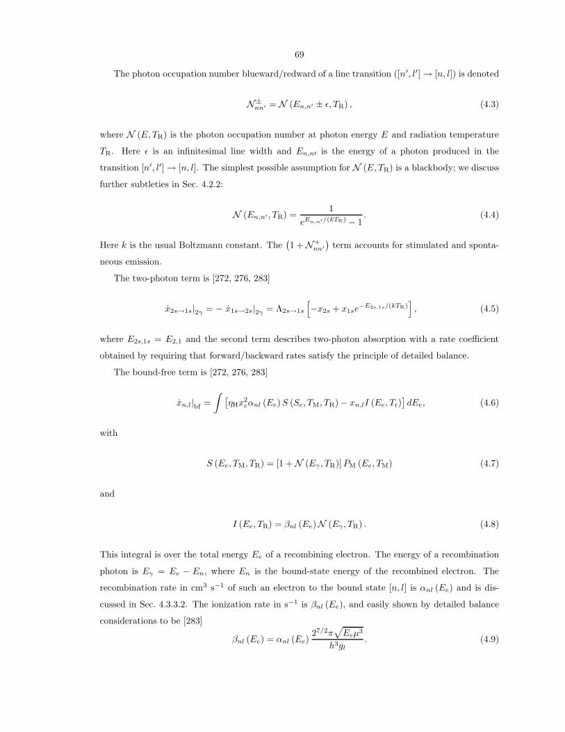
69

The photon occupation number blueward/redward of a line transition ([n′, l′] → [n, l]) is denoted

N±nn′ = N (En,n′ ± ε, TR) , (4.3)

where N (E, TR) is the photon occupation number at photon energy E and radiation temperature

TR. Here ε is an infinitesimal line width and En,n′ is the energy of a photon produced in the

transition [n′, l′] → [n, l]. The simplest possible assumption for N (E, TR) is a blackbody; we discuss

further subtleties in Sec. 4.2.2:

N (En,n′ , TR) =1

eEn,n′/(kTR) − 1. (4.4)

Here k is the usual Boltzmann constant. The(

1 +N+nn′

)

term accounts for stimulated and sponta-

neous emission.

The two-photon term is [272, 276, 283]

x2s→1s|2γ = − x1s→2s|2γ = Λ2s→1s

[

−x2s + x1se−E2s,1s/(kTR)

]

, (4.5)

where E2s,1s = E2,1 and the second term describes two-photon absorption with a rate coefficient

obtained by requiring that forward/backward rates satisfy the principle of detailed balance.

The bound-free term is [272, 276, 283]

xn,l|bf =

∫

[

ηHx2eαnl (Ee)S (Se, TM, TR)− xn,lI (Ee, Tr)

]

dEe, (4.6)

with

S (Ee, TM, TR) = [1 +N (Eγ , TR)]PM (Ee, TM) (4.7)

and

I (Ee, TR) = βnl (Ee)N (Eγ , TR) . (4.8)

This integral is over the total energy Ee of a recombining electron. The energy of a recombination

photon is Eγ = Ee − En, where En is the bound-state energy of the recombined electron. The

recombination rate in cm3 s−1 of such an electron to the bound state [n, l] is αnl (Ee) and is dis-

cussed in Sec. 4.3.3.2. The ionization rate in s−1 is βnl (Ee), and easily shown by detailed balance

considerations to be [283]

βnl (Ee) = αnl (Ee)27/2π

√

Eeµ3

h3gl. (4.9)

70

The free-electron abundance is xe = ηe/ηH, where ηe is the free-electron density. We restrict our

attention to times after helium recombination, and so the free proton abundance xp = xe. The net

bound-free rate [Eq. (4.6)] includes both spontaneous and stimulated recombination. The electron

energy distribution is a Maxwellian with matter temperature TM:

PM (TM , Ee) = 2

√

Ee

π (kTM)3 e−Ee/(kTM). (4.10)

4.2.2 Radiative transfer and escape probabilities

Numerically solving the radiative transfer problem is computationally intensive, but tremendous

simplification can be achieved with the Sobolev escape probability formalism, also known as the

Sobolev approximation [279]. The Hubble flow can be used to define a lengthscale over which the

bulk flow induces a velocity change equal to the thermal velocity: L =√

3kTM/matom/H(TR), where

H (TR) is the value of the Hubble expansion parameter when the radiation has temperature TR and

matom is the mass of an atom [276]. The conditions of the Sobolev approximation are [276, 279, 292]:

(i) L is much smaller than the typical length scales over which cosmological quantities vary, (ii) L/c

is much smaller than the typical time scales over which cosmological quantities vary, (iii) complete

frequency distribution— the rest-frame frequency of an outgoing scattered photon ν does not depend

on the incoming frequency ν ′— and (iv) no other emission, absorption, or scattering processes

occur in the vicinity of the line. Corrections to the Sobolev approximation result from diffusion

around resonance lines [295, 296], atomic recoil [292, 297], Thomson scattering near resonances

[298, 299], and overlap of the higher Ly series lines, leading to important corrections to cosmological

recombination calculations. In this work, however, we work in the Sobolev approximation to focus

on other physical effects.

In the Sobolev approximation, the escape probability for photons produced in the downward

transition [n′, l′] → [n, l] is [276]

P l,l′

n,n′ =1− e−τ l,l′

n,n′

τ l,l′

n,n′

, (4.11)

where the Sobolev optical depth is given by

τ l,l′

n,n′ =c3ηH

8πHν3n,n′

Al,l′

n,n′

(

gl′

glxn,l − xn′,l′

)

, (4.12)

with transition frequency

νn,n′ =En,n′

h=IHh

∣

∣

∣

∣

1

n2− 1

n′2

∣

∣

∣

∣

. (4.13)

Correct expressions for n′ < n are obtained by reversing arguments. During cosmological recombi-

nation, transitions between excited states are optically thin (P l,l′

n,n′ ≥ 0.99972) [283], and so we set

71

P l,l′

n,n′ = 1 in our calculations for non-Lyman lines. The solution for the radiation field near isolated

Lyn lines has the approximate analytic solution [300]

N−n1 = N eq

n1 +(

N+n1 −N eq

n1

)

e−τ ll′

n1

N eqn1 ≡

xnp

3x1s. (4.14)

Transitions in the Lyman (Ly) series (n′ > n = 1, l′ = 1, l = 0) are optically thick (τ l,l′

n,n′ 1)

[283], and so P 0,11,n′ ' 1/τ0,1

1,n′ . Ly transitions cannot, however, be ignored in the recombination

calculation, as the rate at which atoms find their way to the ground state through the redshifting

of resonance photons, P 0,11,n′A

0,11,n′ is comparable to Λ2s→1s and other two-photon rates [283]. Strictly

speaking, τ0,11,n′ depends on xn′,1, and so one should solve for xn′,1 and then iteratively improve the

solution. The populations of the excited states, however, are very small and the maximum resulting

correction to the optical depth is 2 × 10−12 (for n′ = 2, z = 1600) [283]. We thus drop the second

term in Eq. (4.12), simplifying our computation by working in the approximation where the Lyman-

n (Lyn) line optical depth depends only on the ground-state population and not on the excited-state

populations.

Another aspect of the Lyman-series lines is feedback: a photon that escapes from the Lyn

(np → 1s) line will redshift into the Ly(n− 1) line and be reabsorbed. RecSparse has the ability

to implement the resulting feedback, using the iterative technique of Ref. [300]. This slows down

the code by a factor of a few, however, and so to efficiently focus on the nmax problem, we turned

feedback off. For the high Lyman lines, feedback is almost instantaneous: the Universe expands

by a factor of ∆ ln a ≈ 2n−3 during the time it takes to redshift from Lyn to Ly(n − 1). In the

instantaneous-feedback limit, the Lyn lines do not lead to a net flux of H atoms to the ground state.

To approximate this net effect we turned off Lyman transitions with n > 3; this leads to a smaller

error than would result from leaving these transitions on but disabling feedback. Previous tests

using the code of Ref. [292] show resulting errors in the recombination history at the ≈ 1% level; in

any case, this should only weakly be related to the nmax problem. All of the recombination histories

and plots in this chapter were produced by running RecSparse with both feedback and Lyman

transitions from n > 3 disabled, unless noted otherwise. Using the toolkit provided by RecSparse,

we are also exploring extensions to the Sobolev approximation.

4.2.2.1 Line overlap

It is a well known fact that at high n, the separation between adjacent Ly series lines shrink:

νn+1 − νn =IHh

[

1

n2− 1

(n+ 1)2

]

' 2IHhn3

. (4.15)

72

The thermal motion of atoms leads to Doppler broadening of the line, and so it is clear that at

any given temperature, there is a transition value n = no above which neighboring lines overlap.

In other words, the fates accessible to a photon produced in the overlapping regime of the Ly-n

resonance extend beyond re-absorption by the Ly-n line or escape (until red-shifting brings it into

the next Lyman line). This photon may also be immediately re-absorbed by other nearby Ly lines

[e.g. Ly-(n+ 1), Ly-(n− 1), and so on]. The Doppler width of a Lyman line is given by

∆νn = νn

√

2kTM

mpc2, (4.16)

where mp is the proton mass. We can obtain the line-overlap condition by demanding that ∆νn ∼>

νn+1 − νn, thus yielding

n ∼> no ≡ 44

(

TM

3000 K

)−1/6

(4.17)

as the requirement for overlap of adjacent Ly lines [291]. For yet higher n, high-lying Ly lines will

even overlap with the continuum. Similar arguments then lead to the condition

n ∼> nc ≡ 206

(

TM

3000 K

)−1/4

(4.18)

for Ly line overlap with the continuum. Once this condition kicks in, the large reservoir of ionizing

photons could feed the recombination network through an additional channel due to overlap between

the continuum and the Lyman series, pumping atoms into excited states, but also providing a new

channel to the ground state. Modern recombination codes routinely probe n > nmax = 100 [7–9, 44].

Indeed, in the work described in this chapter and later work by others, substantial effort was devoted

to determining the value of nmax required for adequate convergence in the recombination history.

Since Ly line overlap becomes important at high n, it is important to properly treat the effect of

line overlap on recombination.

Line overlap explicitly breaks assumption iv) of the Sobolev approximation: (iv) no other emis-

sion, absorption, or scattering processes occur in the vicinity of the line. Fortunately, the same

techniques used to solve for the occupation number N (En,n′ ± ε) in the Sobolev approximation

may be readily generalized. The results may be written in a form that lends itself to straightforward

numerical integration, as shown in recent work by Y. Ali-Haımoud [291]. Qualitatively speaking, for

n ∼> no (though it turns out small corrections due to overlap already appear at n ∼> 22), the solution

for the occupation number [Eq. (4.14)] must be replaced with a sum over overlapping Lyman lines,

and the portion of the rate matrix corresponding to np→ n′p transitions must be adjusted to include

overlap terms. Using the RecSparse toolkit, we are working on the inclusion of these corrections

[291]. Preliminary results indicate that the correction to xe (z) ∼< 10−5 for n ∼< 150, leaving most of

73

the conclusions in this chapter unchanged.

4.2.3 Matter and radiation temperatures

Electrons, though non-relativistic during recombination, interact with photons through Thompson

scattering. As a result, they do not follow the simple adiabatic scaling TM ∝ a−2, where a is the

cosmological scale factor. Rather, the matter temperature evolution equation is [277, 278, 301]

TM = −2HTM +8xeσTaRT

4R

3 (1 + fHe + xe)mec(TR − TM) . (4.19)

The second term represents the coupling of electrons to photons through Compton scattering. At

early times, the second term dwarfs the others and TM = TR, while after matter and radiation cease

efficiently interacting, TM ∝ a−2. The Compton equilibration time is

tcomp =3 (1 + fHe + xe)mec

2

8xe (cσT) aRT 4R

. (4.20)

When tcomp 1/H(z), there is a convenient first-order asymptotic solution, derived in Ref. [283]

using an appropriate integrating factor:

TM

TR' 1− 3 (1 + fHe + xe)mecH

8xeσTaRT 4R

. (4.21)

Here σT is the Thompson scattering cross section, aR is the radiation constant, fHe = YHe/ [r (1− YHe)]

is the He:H ratio by number, and r = mHe/mH ' 3.9715 is the He:H atomic mass ratio. We neglect

subdominant processes, such as free-free, line, photo-recombination and collisional ionization cool-

ing, as well as photoionization and collisional recombination heating [276]. RecSparse output for

the evolution of the ratio TM/TR is shown for two cases in Fig. 4.1, one for which the asymptotic

solution is used at all times, and one for the numerical solution to Eq. (4.19) is used after z = 500.

We see that the error in the asymptotic solution is less than 10% of TM/TR until z ∼ 200. It may

seem surprising that TM stays so close to Tγ long after Thompson scattering freezes out at the SLS

(z ∼ 1100). After all, this is nominally when photons decouple from electrons. It is important to

remember, however, that ηγ/ηb 1, where ηγ and ηb are the number densities of photons and

baryons today, respectively. Until z ∼ 500, a free electron can thus easily ‘find’ a photon, while a

photon is unlikely to encounter a free electron. As a result, TM ∼ TR long after one might naively

expect this to cease being the case. Unless noted otherwise for certain specific illustrative cases, we

use the following prescription to evolve TM/TR for the RecSparse results presented in this chapter:

for z ≤ 500, we solve Eq. (4.19) numerically, while for z > 500, we apply Eq. (4.21).

74

Figure 4.1 Evolution of the ratio of matter/radiation temperatures TM/TR as a function of redshift zfor a RecSparse run with nmax = 100. The left panel shows TM/TR. The black curve correspondsto the asymptotic solution [Eq. (4.21)] for z > 500 and the numerical solution to Eq. (4.19) forz ≤ 500. The right curve shows how the fractional error ∆ (TM/TR) / (TM/TR) of the asymptotic

solution evolves with z, where ∆ (TM/TR) ≡[

(TM/TR)|numeric − (TM/TR)|asymptotic

]

.

4.2.4 The steady-state approximation

The wide range of disparate time scales in this problem would naively necessitate a stiff differential

equation solver. This computational expense can be avoided by repackaging Eqs. (4.1), (4.2),and

(4.5)-(4.8). These equations may be rewritten for excited states as ([n, l] 6= [1, 0])

xn,l = −∑

n′l′

T l,l′

n,n′xn′,l′ + sn,l, (4.22)

with

T l,l′

n,n′ = δl,l′

n,n′

Inl + γnl +∑

n′′,l′′

Γl′′,l′

n′′,n′

− Γl,l′

n,n′ , (4.23)

where the integrated photoionization rate from [n, l] is

Inl =

∫

βnl (Ee) I (Ee, TR) dEe (4.24)

and Γl,l′

n,n′ is defined in Eq. (4.2).

The downward flux to the ground state is

γnl = A0,11,nP

0,11,n

(

1 +N+1n

)

δl,1 + Λ2s,1sδl,0n,2, (4.25)

75

where the first term describes Lyn series transitions (stimulated and spontaneous) while the second

accounts for the [2, 0] → [1, 0] two-photon transition. Kronecker delta symbols (δl,l′

n,n′ and δl,l′) are

employed throughout to enforce [n, l] = [n′, l′] and l = l′).

The source term snl includes flux from the ground state and direct recombination into the state

[n, l]:

sn,l = ηHx2e

∫

αnl (Ee)S (Ee, TM, TR) dEe + x1sΛ2s,1se−E2s,1s/(kTR)δl,0

n,2

+ x1sglA0,11,nP

0,11,nN+

1nδl,1/2. (4.26)

This can also be rewritten in matrix notation: d~x/dt = −T~x + ~s, where T is the matrix of rates

with components given by Eq. (4.23).

The left-hand side of Eq. (4.22) is associated with the recombination time scale, while both

terms on the right-hand side are associated with much shorter atomic time scales. For example, the

longest lifetimes in the recombination problem are those of the 2s and 2p states (Λ2s,1s ∼ 10 s and

A2p,1sP2p,1s ∼ 1 s when Ly-α optical depth peaks at τ ∼ 6 × 108), considerably shorter than the

recombination time scale of trec ∼ 1012 s. Thus we make a steady-state approximation, xnl = 0,

which is formally valid because the reciprocal of the minimum eigenvalue of T peaks at 0.8 s, which

is ∼ 10−12 of the duration of recombination. Thus the excited-state abundances are given by

~x ' T−1~s. (4.27)

The rates in T and ~s depend on xe, x1s, TM, TR, and N . The ground-state population is given by

x1s = 1− xe −∑

[n,l]6=[1,0] xn,l, but since excited-state populations are small (xn,l < 10−13), x1s can

be eliminated from Eq. (4.26) using the approximation x1s ' 1 − xe. We can then solve for the

evolution of xe, leaving out ineffective direct recombinations to the ground state:

xe ' −x1s = x1sΛ2s,1se−E2s,1s/(kTR) −

∑

[n,l]6=[1,0]

(

γnlxn,l −gl

2A0,1

1,nP0,11,nN1nx1sδl,1

)

. (4.28)

The steady-state approximation thus allows us to convert a stiff system of ordinary differential

equations into a large system of coupled linear algebraic equations, along with a single ordinary

differential equation.

4.3 Recombination with high-n states

The original “effective 3-level atom” (TLA) treatments of cosmological recombination in Refs. [272,

273] were built on the assumption that the primary bottlenecks to effective recombination are the

slow 2s → 1s transition rate and the reabsorption of 2p → 1s resonance photons by the optically

76

thick plasma. Other crucial assumptions included radiative equilibrium between excited states,

xn = x2e−(En−E2)/(kTR)n2/4 if n > 2, (4.29)

xn ≡∑

l<n−1

xn,l, (4.30)

and statistical equilibrium between angular momentum sublevels:

xn,l = xn(2l+ 1)

n2. (4.31)

Recombination to higher excited states was included through an effective “Case B” total recombi-

nation constant αB(T ) (recombinations to the ground state are omitted) [272, 276].

As the radiation field cools and the baryon density falls at late times, the transitions coupling

high-n to low-n become inefficient, as do those coupling different l sublevels with the same n. This

leads to a breakdown of statistical equilibrium (note however that the steady-state approximation

is still valid), and so Eqs. (4.30) and (4.31) cease to apply. In Ref. [276], Eq. (4.30) is relaxed while

Eq. (4.31) is still imposed, and ∼ 10% corrections to the TLA prediction for xe(z) result. At late

times, nonequilibrium effects cause a net flux downward from states with quantum number n to the

ground state, accelerating recombination. The inclusion of progressively more shells increases the

number of downward cascade channels to the ground state for continuum electrons. Thus higher

nmax leads to faster recombination and lower xe(z). Reference [276] reports results for nmax as high

as 300. The Lyman (np→ 1s) transitions from very high-n states overlap with the Lyman continuum

due to thermal broadening. Ref. [276] uses this fact to argue that the high-n states themselves are

indistinguishable from the continuum, and that there is thus no need to go past n = 300. This is an

incorrect line of reasoning, and it is important to correctly treat the problem of high-n convergence

in cosmological recombination.

4.3.1 Are high-n states well-defined and physical?

The real question as to whether the different values of n are well defined is whether the broadening

of the state, ~/t (where t is the lifetime) is larger than the splitting of adjacent energy levels,

∆Esplit ≈ 2IHn−3. The intrinsic broadening for a typical level with l/n ∼ O(1) is [302]

∆E ∼ ~/t ∼ α3IHn5

, (4.32)

77

where α ' 1/137 is the usual fine structure constant. For l = 1 states, the intrinsic width is

dominated by Lyman-series transitions, and so [303]

∆E ∼ α3IHn3

. (4.33)

In the l/n ∼ O(1) case, the condition ∆E ∆Esplit imposes the condition n2 α3 ∼ 10−6, which

is clearly satisfied for any physical n. In the case of the l = 1 states, ∆E ∆Esplit imposes the

consistency condition 2 α3, which is also obviously always true. Thus ∆E ∆Esplit and so

these extremely high-n energy levels are well defined; indeed, transitions between highly excited

states in such nonequilibrium plasmas are seen in interstellar H ii regions and are a useful diagnostic

of physical conditions [304]. States in the intermediate region between l = 1 and l/n ∼ O (1) are

bracketed by the range just described and are thus also well defined.

For extremely large n, the above physical argument may break down because of additional broad-

ening contributed by interactions with the radiation field or the plasma. In the case of broadening

due to stimulated emission and absorption, the additional (radiative) contribution to the width is

∆E ∼ ~

∑

n′,l′=l±1

Al′,ln′,nN (En,n′) . (4.34)

The Lyn lines are optically thick and thus N (E1,n) ' xnp/ (3x1s), as can be seen from Eq. (4.14).

As a result, N (E1,n) < 10−13 [283] and Lyman-series transitions may be neglected from the sum in

Eq. (4.34).

When hνn′,n kTR, deep in the Wien tail of the microwave blackbody, photon occupation

numbers are highly suppressed, and so non-Lyman transitions with ∆n = n′ − n n may also be

neglected in Eq. (4.34). When hνn′,n kTR and ∆n n, the denominator of Eq. (4.4) may be

expanded to yield

N (En′,n) ' kTR

hνn′,n' kTR

IH

1∣

∣

1n′2 − 1

n2

∣

∣

' kTRn3

2IH∆n, (4.35)

where the last step follows from expanding |1/n′2 − 1/n2| for ∆n n. Using the asymptotic

expression for∑

l′,lAl′,ln′,n (when ∆n n) in Ref. [305], we then obtain

∆E ∼ 16α3kTR

3π√

3n2

∞∑

∆n=1

(

1

∆n

)2

=8πα3kTR

9√

3n2. (4.36)

Requiring that ∆E ∆Esplit then imposes the condition

n nstim,

nstim ≡ 9√

3

4πα3

IHkT0 (1 + z)

, (4.37)

78

where T0 is the CMB temperature today.

At sufficiently high distances from the atomic nucleus, the Coulomb potential from charged par-

ticles (predominantly electrons and protons in the primordial plasma) clustered around the nucleus

will be comparable to the Coulomb potential of the hydrogen nucleus. This shielding occurs on the

Debye length scale [306]:

RD =

(

kTM

4πηee2

)1/2

. (4.38)

Here e is the norm of the electron charge. This shielding may be ignored as long as the expectation

value 〈r2〉nl RD. Otherwise, the contribution of free charge carriers in the plasma to the potential

within the bound-electron radius may not be ignored, and for r ∼> RD, a distorted potential, such as

the Debye-Huckel potential, should be used to properly estimate transition energies and rates [307].

For a Coulomb hydrogen atom [303],

〈r2〉nl = a20n

2

[

5n2 + 1− 3l(l+ 1)

2

]

. (4.39)

For a strict bound on the range of n for which this effect may be ignored, we wish the maximum value

of 〈r2〉nl given by Eq. (4.39) to obey the constraint 〈r2〉nl RD. We thus apply this inequality

with the choice l = 0, yielding the constraint

n4 n4Debye

n4Debye ≡ kTM

10πxeηHxee2a20

. (4.40)

In a sufficiently dense gas, loosely bound (high-n) electrons could find themselves close enough

to nearby charge carriers that the energy shells are significantly distorted. In fact, this ‘collisional

broadening’ may be strong enough that the energy levels become blended. This is essentially the well

known Stark effect, and has been observed in spectral lines from stellar atmospheres. If the zero of a

bound electron’s energy is set at infinite distance from the hydrogen nucleus, the interaction energy

with a neighboring charge carrier is ∆E ∼ e2√

〈r2〉nl/r2p, where rp is the typical distance between

the perturbing charge carrier and the bound electron. If we demand, as before, that ∆E ∆Esplit,

then we obtain the condition [308]

n5 n5Stark,

n5Stark ≡

√

2

5

1

(a30ηe)

2/3. (4.41)

In Fig. 4.2, we show nstim, nDebye and nStark as computed using Eqs. (4.37), (4.40), and (4.41).

Using Fig. 4.2, we verify that during the recombination epoch, radiation and plasma induced dis-

tortions of atomic energy levels may be ignored, as long as n ∼< 103, a condition respected by all

79

Figure 4.2 Transition shell numbers nstim, nDebye, and nStark. For n > nmax, the broadening ofspectral lines due to stimulated emission/absorption, Debye screening, and collisions becomes com-parable to the inter-level spacing. This plot was produced using a RecSparse run with nmax = 30and TM given by Eq. 4.21.

RecSparse runs shown in this chapter. All the same, it is instructive to estimate the ‘size’ of the

highly excited atoms we model in our computation. Roughly, r ∼ a0n2 = 2µm for n = 200. These

are very big atoms! The constraints on stimulated emission and Debye screening are most easily

satisfied (n 108 and n 104, respectively), while the constraint on collisional broadening is more

marginal. For the nmax values considered in this paper, collisional broadening is still two orders of

magnitude smaller than the inter-level spacing; it is conceivable, however, that future computations

of recombination (with nmax higher by a factor of 3 or more) will require a more careful treatment

of plasma effects. For the purposes of predicting xe(z) precisely enough for Planck, we may proceed

onward and ignore broadening by stimulated emission/absorption, Debye screening, and collisional

broadening. All we have established here is that the energy levels are well defined in spite of these

potential complications. We must certainly still include stimulated emission/absorption in our rate

equations [as done through Eq. (4.2)], and we may have to include l-changing collisions as well (an

issue addressed in Sec. 4.5.1.2).

80

4.3.2 Computational challenges

Recent work [7, 8] shows that additional ∼ 1% corrections to xe(z) arise when Eq. (4.31) is not

imposed and the populations of l sublevels are followed separately. Bottlenecks to decays from high

l imposed by l′ = l±1 slow down cascades to the ground state, and thus lead to slower recombination.

In this case, the sidelength of T is N = O(

n2max

)

. Since the number of computational steps needed

to invert a matrix is generically a N 3 process, the computational time needed for a single ODE time

step in the recombination time will be proportional to n6max.

As noted in Ref. [8], a recombination calculation with nmax = 100 already takes ∼ 6 days on a

standard workstation. It this thus difficult to explore how quickly xe (z) converges for progressively

higher values of nmax. Even between nmax = 80 and nmax = 100, ∼ 1% changes are seen in the

TT and EE multipole moments (C`s) of the CMB. In Ref. [40], the results of Ref. [8] are used

to explore the effect of progressively higher nmax on CMB C`s. In that work, it is noted that the

fractional difference between the C`s for nmax = 60 and nmax = 120 falls within a heuristic Planck

performance benchmark. Higher values of nmax come even closer to the fiducial case of nmax = 120,

a fact used to argue that even nmax = 60 recombination is adequate for Planck data analysis.

From the Cauchy convergence criterion, however, we know that a meaningful convergence test

requires a comparison between successive members in a sequence. Using the results of Ref. [8]

alone, the question of convergence with nmax thus remains open. In spite of the computational

challenge, it is thus crucial to push the calculation to sufficiently high nmax that corrections to xe(z)

from remaining n > nmax are so small that they do not effect CTT` or CEE

` at a level statistically

significant compared to the predicted Planck sample variance (e.g., several parts in 104 for l > 1000)

[299]. There are two challenges in treating such a big multilevel atom. The first is the calculation of

atomic transition rates at extremely high n; this is tractable because of some convenient recursion

relations. The second is simultaneously evolving the populations of nmax (nmax + 1) /2 states. We

discuss these in turn below.

4.3.3 Rates

Here we discuss the Einstein coefficients for dipole bound-bound and bound-free transitions in atomic

hydrogen, which are used in our recombination computation. We omit reduced-mass corrections to

make a consistent comparison with Refs. [302, 309–312], but include them when calculating actual

recombination histories.

81

4.3.3.1 Bound-bound rates

The spontaneous electric dipole transition rate (1)Al′,ln′,n for a nonrelativistic hydrogen atom is given

by [313]

(1)Al,l′

n,n′ =64π4ν3

n,n′

3hc3max(l, l′)

2l + 1e2a2

0

∣

∣

∣

(1)X l,l′

n,n′

∣

∣

∣

2

, (4.42)

(1)X l,l′

n,n′ ≡[∫ ∞

0

x3Rn′l′(x)Rnl(x)dx

]

, (4.43)

where e is the absolute value of the charge of an electron, h is Planck’s constant, and (p)X l,l′

n,n′

denotes the radial matrix element between the states [n, l] and [n′, l′] at order p in the multipole

expansion. For example, (2)Al′,ln′,n denotes the quadrupole rate, and so on.The restriction l′ = l ± 1

enforces electric dipole selection rules. Here Rnl(x) is the radial wave function of an electron in a

hydrogen atom, with principal quantum number n and angular momentum quantum number l, at

a dimensionless distance x. All dimensionless distances are measured in terms of a0. For Coulomb

wave functions, this integration yields the Gordon formula [313]:

(1)X l,l′

n,n′ =(−1)

n′−l

4 (2l− 1)!

√

(n+ l)! (n′ + l − 1)!

(n− l − 1)! (n′ − l)!(4nn′)l+1

(n+ n′)n+n′(n− n′)n+n′−2l−2

W (n, n′, l) , (4.44)

where l′ = l − 1,

W (n, n′, l) = 2F1 (u,−n′ + l, 2l, w)−(

n− n′n+ n′

)2

2F1 (v,−n′ + l, 2l, w) , (4.45)

with u = −n + l + 1, v = −n + l − 1, and w = −4nn′/ (n′ − n)2. Here 2F1 (a, b, c;x) is Gauss’s

hypergeometric function for integer a, b, and c, evaluated using the recursion relationship

(a− c) 2F1 (a− 1, b, c;x) = a(1− x) [2F1 (a, b, c;x)

−2F1 (a+ 1, b, c;x)] + (a+ bx− c) 2F1 (a, b, c;x) , (4.46)

with initial conditions

2F1 (0, b, c;x) = 1, 2F1 (−1, b, c;x) = 1− bx

c. (4.47)

We use Eqs. (4.43)-(4.47) to calculate bound-bound transition rates at the beginning of a MLA

computation, storing them for easy and repeated access.

We compared the resulting radial matrix elements with several values for high n in Ref. [309]

and found agreement to all 3 published digits. We calculated oscillator strengths and compared with

Ref. [310] (all transitions with n and n′ were evaluated, as was the entire Balmer series for n ≤ 60)

82

and found agreement to all 6 published digits. We also compared with the results in Ref. [311]

(in which oscillator strengths were computed up to n = 500 for ∆n ≤ 5) and found agreement to

5 digits. We attribute the difference in oscillator strengths to the fact that a polynomial expansion

of 2F1 was used in Ref. [311], rather than the more stable recursion relationship. We also compared

with the dipole one-photon rates used for the nmax = 30 MLA computation of Ref. [283]. Most rates

agreed to 7 or more significant figures. Transition rates between s and p orbitals only agreed to ∼ 5

significant figures. We ran our MLA model using the rates of Ref. [283] and verified that these small

disagreements do not lead to any differences in xe (z) at the desired level of accuracy. Given the high

quantum numbers considered, it was important to verify that no numerical instability plagues our

numerical implementation of these recursions. We thus checked matrix elements computed using

Eqs. (4.44)-(4.47) against values estimated using the WKB approximation, as detailed in Appendix

C.

4.3.3.2 Bound-free rates

Bound-free rates are evaluated using the same principle, but one of the two states used to evaluate

matrix elements must be a continuum Coulomb wave function. The resulting matrix element is [314]

gl,l′

n,κ =1

n2

∫ ∞

0

x3Rnl(x)Fκl′ (x)dx, (4.48)

where Fκl′ is the continuum Coulomb wave function for a recombining photoelectron with angular

momentum quantum number l′ and dimensionless energy κ2 = Ee/IH = hνIH− 1/n2. The energy of

the outgoing photon is hν. This integral may also be evaluated in terms of hypergeometric functions,

which in turn yields a recursion relationship for gl,l′

n,κ [312]:

Gl,l′

n,κ ≡ gl,l′

n,κ

(2n)l−nq

(n+l)!(n−l−1)!

Q

l′

s=0(1+s2κ2), (4.49)

Gl−2,l−1n,κ =

[

4(

n2 − l2)

+ l (2l− 1)(

1 + n2κ2)]

Gl−1,ln,κ − 4n2

(

n2 − l2)

[

1 + (l + 1)2κ2]

Gl,l+1n,κ ,

Gl−1,l−2n,κ =

[

4(

n2 − l2)

+ l (2l+ 1)(

1 + n2κ2)]

Gl,l−1n,κ − 4n2

[

n2 − (l + 1)2]

(

1 + l2κ2)

Gl+1,ln,κ .

The initial conditions of the recursion are [312]

Gn−1,nn,0 =

√

π

2

8n

(2n− 1)!(4n)

ne−2n, (4.50)

Gn−1,nn,κ =

e2n−2κ−1 atan(nκ)

√

1− e− 2πκ (1 + n2κ2)

n+2Gn−1,n

n,0 ,

Gn−2,n−1n,κ = (2n− 1)

(

1 + n2κ2)

nGn−1,nn,κ ,

Gn−1,n−2n,κ =

(

1 + n2κ2

2n

)

Gn−1,nn,κ .

83

These matrix elements are tabulated at the beginning of each MLA run for all l < n ≤ nmax,

and 10−25 ≤ κ2n2 ≤ 4.96× 108; this range of κ is partitioned into 50 logarithmically spaced bins,

with each bin containing 11 equally spaced κ values. Bound-free matrix elements were compared

with tabulated values for low n in Ref. [312] and agreed to all 4 listed digits. Matrix elements were

also compared with those used in Ref. [283]; we found agreement to one part in 107, aside from s−ptransitions, as already discussed.

The recombination rate to [n, l] as a function of energy is then

αnl (Ee) =4√πα4a2

0cI3/2H

3n2 (kTM)3/2

∑

l′=l±1

max l, l′Θl,l′

n,κ, (4.51)

with

Θl,l′

n,κ =

(

1 +n2Ee

IH

)3∣

∣

∣gl,l′

n,κ

∣

∣

∣

2

. (4.52)

At each value of TM , the tabulated matrix elements, Eqs. (4.6) and (4.51) are used to calcu-

late thermally averaged recombination rates, using an 11-point Newton-Cotes [315] formula for the

integration and neglecting stimulated emission. Large bins are added into the integral until it has

converged to a fractional precision of 5 × 10−15. We compared our values with integrated rates

tabulated in Ref. [312] and found agreement to all 4 listed digits. Comparing with the rates used in

Ref. [283], we found agreement to one part in 107, aside from s-p transitions.

In Saha equilibrium,

η2eαnl (Ee) [1 +N (Eγ , TR)]PM (Ee, TM) = ηHxn,lN (Eγ , TR)βnl (Eγ) , (4.53)

and so by the principle of detailed balance,

∫

dEeβnl (Eγ) =x2

eηHxn,l

∫

dEeαnl (Ee)[1 +N (Eγ , TR)]

N (Eγ , TR)

∣

∣

∣

∣

eq

PM (Ee) . (4.54)

We verified that our computed thermally averaged recombination and ionization rates satisfied

this equality to machine precision. We also checked bound-free matrix elements computed using

Eq. (4.50) against values estimated using the WKB approximation, as detailed in the Appendix C.

4.3.4 Sparse-matrix technique

The key to making the recombination problem tractable for high values of nmax is the sparsity of

Eqs. (4.22) and (4.23). Dipole selection rules only allow coupling of states with angular momentum

quantum numbers l and l′ if l′ = l ± 1. It is easiest to understand how sparsity simplifies the

84

Figure 4.3 Schematic of the sparse rate matrix T with components given by Eq. (4.23) and submatrixbuilding blocks given by Eq. (4.58). Boldface zeroes denote block matrices of all zeros, and enforcethe dipole selection rule that the initial state l′ angular momentum obeys l′ = l±1, where l is the finalstate angular momentum. The submatrix Mll′ has dimension (nmax − nmin + 1)×(nmax − n′min + 1),where nmin = 2 if l = 0, and nmin = l+ 1 if l > 0. Note that submatrices Ml,l on the block diagonalof the larger rate matrix T are themselves diagonal, as seen from Eq. (4.58) and the fact that in the

purely radiative case, Γl,l′

n,n′ = 0 if n 6= n′ and l = l′.

problem with a slight change of notation. We can compose the vector ~x (with components xn,l) of

excited-state populations, as

~x =

~v0

~v1

...

~vlmax

, (4.55)

where lmax = nmax−1 and ~vl denotes a vector of the populations of all states with angular momentum

l, except for the 1s state. Specifically,

~vl =

xnmin,l

xnmin+1,l

...

xnmax,l

, (4.56)

where

nmin =

2 if l = 0,

l + 1 if l 6= 0.(4.57)

The source vector ~s can similarly be written by concatenating source vectors ~sl; each ~sl feeds all

states with angular momentum l.

The rate matrix may be similarly built of submatrices Ml,l′ , as illustrated in Fig. 4.3. The

complete rate matrix is block tridiagonal, and the blocks decrease in dimension as l increases. The

85

matrix Ml,l′ has components

Mn,n′

l,l′ = δl,l′

n,n′

Inl + γnl +∑

n′′,l′′

Γl′′,l′

n′′,n′

− Γl,l′

n,n′ . (4.58)

In the steady-state approximation, Eq. (4.22) can be rewritten as a system of matrix equations.

If l = 0,

M0,0~v0 + M0,1~v1 = ~s0. (4.59)

If 0 < l < lmax,

Ml,l−1~vl−1 + Ml,l~vl + Ml,l+1~vl+1 = ~sl. (4.60)

To close the system, we must truncate the hierarchy by excluding states with n > nmax as both

sources and sinks, which is equivalent to setting Al,l±1n,n′ = 0 for max n, n′ > nmax. Then for

l = lmax,

Mlmax,lmax−1~vlmax−1 + Mlmax,lmax~vlmax = ~slmax . (4.61)

It might be possible to approximate the correction due to this truncation error, using asymptotic

expressions for Al,l±1n,n′ and Saha equilibrium abundances for n > nmax. This will only work if nmax is

sufficiently high for nearly perfect equilibrium Saha equilibrium to hold between states with n > nmax

and the continuum.

At any given time step, the actual quantity of interest is not the inverse T−1 of the rate matrix

but the solution set ~vl to the steady-state rate equations. The closed form solution to Eqs. (4.59)-

(4.61) is

~vl = Kl

[

~sl −Ml,l+1~vl+1 +l−1∑

l′=0

(−1)l′−l Sl,l′~sl′

]

, (4.62)

if l < lmax. If l = lmax, then

~vl = Kl

[

~sl +

l−1∑

l′=0

(−1)l′−l

Sl,l′~sl′

]

. (4.63)

Here

Kl =

M−100 if l = 0,

(Ml,l −Ml,l−1Kl−1Ml−1,l)−1

if l > 0,(4.64)

and

Sl,i =

Ml,l−1Kl−1 if i = l − 1,

Sl,i+1Mi+1,iKi if i < l − 1.(4.65)

Our new MLA code, RecSparse, operationally implements this solution at each time step as follows:

1. Using the values of TR and xe, TM is calculated using the results of Sec. 4.2.2.

86

2. All relevant Ml,l′ and ~sl are computed using Eqs. (4.58) and (4.26) and stored.

3. All Kl and Sl,i are computed using Eqs. (4.64)-(4.65) and stored.

4. Equation (4.63) is applied to obtain the solution for ~vlmax .

5. Equation (4.62) is iterated to obtain the solutions for all ~vl.

The free-electron fraction xe is then evolved forward in time using ~vl and Eq. (4.28). It would

also be interesting to compute the cumulative spectral distortion emitted by the line and continuum

processes responsible for recombination [7, 8, 275, 316]. This fractional perturbation of 10−7 to

the blackbody intensity of the CMB could be detectable with future experiments and would offer

a test both of our understanding of recombination and of new physics behind the surface of last

scattering (e.g., time variation of fundamental constants, energy injection by decaying/annihilating

dark matter) [317–321]. This and the development of a fast code for Planck data analysis including

all the relevant physical effects will be the subject of future work.

4.3.5 Numerical methods

RecSparse begins at z = 1606, assuming Saha equilibrium to compute the initial value of xe and

setting TM as discussed in Sec. 4.2.2. Excited-state populations are obtained using the method

of Sec. 4.3.4. Submatrix inversions are implemented using the double precision routine DGESVX

from the LAPACK library [322]. Time evolution of xe(z) with Eq. (4.28) is implemented using the

5th-order Runge-Kutta-Cash-Karp (RKCK) implementation in Numerical Recipes [323]. The rapid

time scale for return to Saha equilibrium introduces a stiff mode into the equations at early times,

necessitating care in the choice of a stepsize for the integrator. We were able to achieve relative

precision of ε ∼ 10−8 by placing 59 time steps at z ≥ 1538 and 250 steps in the range 200 ≤ z ≤ 1538,

partitioning each interval into equally sized steps in ∆ ln a; relative errors were estimated by halving

step size and comparing values of xe(z) at identical time steps. The computation time tcomp for

RecSparse scales as tcomp ∝ nαmax, where 2 < α < 3. This is an empirical estimate for the range of

nmax that we have explored, and may not extend to higher nmax values. In contrast, for standard

MLA codes, tcomp ∝ n6max. We can calculate recombination histories for nmax = 200 in 4 days on a

standard workstation; this would likely take weeks using a conventional MLA code.

4.4 Extension to electric quadrupole transitions

Early work on recombination highlighted the importance of forbidden transitions, as half of the

hydrogen atoms in the Universe form by way of the 2s → 1s “forbidden” transition [272, 273].

87

Recent work has included additional “forbidden” transitions in the MLA treatment, namely, two-

photon transitions (ns→ 1s and nd→ 1s) in H [280–283], two-photon and spin-forbidden transitions

in He [284–287], as well as electric quadrupole (E2) transitions in He [299, 300].

Until this work, the impact of E2 transitions in H on recombination has not been considered, even

though they are optically thick for transitions to/from the ground state. For optically thick lines, the

overall transition rate is proportional to Al,l′

n,n′/τl,l′

n,n′ . Since τ l,l′

n,n′ ∝ Al,l′

n,n′ , the overall transition rate

is independent of the rate coefficient. Transitions such as electric quadrupoles, which seem “weaker”

judging from rate coefficients alone, can thus be as important as “stronger” transitions, like the

Lyn lines. For example, this is why the semiforbidden He i 591A line is important in cosmological

recombination [299, 300]. We thus include E2 quadrupole transitions in our MLA computation

to properly assess their relevance for cosmological recombination. M1 (magnetic dipole) transition

rates in H are typically suppressed by an additional factor of 107−108, and are thus negligible [324].

4.4.1 Rates

The electric quadrupole (E2) Einstein A-coefficient for transitions from states [n, l] to states [n′, l′]

is [325]:

(2)Al′,ln′,n =

αω5n,n′a

40

15gac4

∣

∣

∣〈nl| |Q(2)| |n′l′〉∣

∣

∣

2

, (4.66)

where the quadrupole matrix element is

〈nl|Q(2) |n′l′〉 = 〈l| |C(2)| |l′〉 (2)X l′,ln′,n. (4.67)

The matrix elements of the reduced angular tensor operator C (2) are given by

〈l| |C(2)| |l′〉 = (−1)l√

glgl′

l 2 l′

0 0 0

, (4.68)

where the last factor is the well-known Wigner-3J symbol. This operator is defined as

〈l| |C(k)| |l′〉 = (−1)l−m

l k l′

−m q m′

−1√

4π

2k + 1〈lm|Ykq (θ, φ) |l′m′〉 . (4.69)

The dimensionless radial quadrupole integral is

(2)X l′,ln′,n =

∫ ∞

0

x4Rn′l′(x)Rnl(x)dx. (4.70)

Thanks to the existence of ladder operators for the radial Coulomb wave functions Rnl(x), these

matrix elements may be derived using convenient recursion relationships [326] illustrated in Appendix

88

D. The radial matrix element for the nd→ 1s transition is a special case of Eq. (B.13) of Ref. [326]

with n′ = 1 [Eq. (D.9) in Appendix D of this thesis]:

(2)X0,21,n = (−1)n−126n4

[

(n+ 2)!

(n− 3)!

]1/2(n− 1)

n−4

(n+ 1)n+4 . (4.71)

We numerically implemented this recursion in RecSparse. We checked special cases of (2)X l′,ln′,n

against values tabulated in Ref. [326], and found agreement to all listed digits. We also compared

(2)Al′,ln′,n with the rates in Ref. [324]. The rates in Ref. [324] result from numerical integration of the

more precise Dirac wave function and so the resulting fractional disagreement of O(

α2)

∼ 5×10−5 is

not surprising. This is a ‘correction to a correction,’ and so our calculated rates should be adequate

for assessing the importance of E2 transitions. We also checked our precise calculated values of

(2)X l′,ln′,n against values estimated using the WKB approximation, as detailed in Appendix D.

4.4.2 Inclusion in multilevel atom code

The obvious way to include quadrupole transitions into our MLA code would be to generalize Eq.

(4.60) to include ∆l = ±2 transitions:

Ml,l+2vl+2 + Ml,l+1vl+1 + Ml,lvl + Ml,l−1vl−1 + Ml,l−2vl−2 = sl. (4.72)

The resulting system is obviously not as sparse as in the dipole case, and solving for all vl would

be computationally more expensive, slowing down the whole MLA code. Since the contribution

from even the largest quadrupole rates may turn out to be small, we pursue a computationally less

expensive approach.

Higher energy E2 transitions will proceed much faster than lower energy ones, since E2 rates

scale as ω5nn′ . In particular, transitions to and from the 1s ground state will dominate any other

quadrupole contributions to the recombination problem, since

(2)A0,21,n

(2)A0,2q,n

∼ ω51n

ω5qn

=

[

q2(

n2 − 1)

n2 − q2

]5

∼> 103 if q ≥ 2. (4.73)

Moreover, the nd → 1s lines are optically thick for small n. We thus restrict our consideration

to nd ↔ 1s transitions, since other quadrupole transitions are “corrections to a correction.” A

further simplification follows if we recall that the Lyn lines are all optically thick [283]. Thus, the

transition nd → 1s is highly probable to be immediately followed by a transition 1s → np. This

yields a net nd → np transition, analogous to an l-changing collision, which occurs with forward

rate (2)Γ0,21,n = xnd

(2)A0,21,n. The reverse process occurs with rate (2)Γ0,2

1,n = xnp(2)A0,2

1,nD, where D is a

factor relating forward and backward rates. If the p and d states were in equilibrium, the two rates

89

would cancel, so by the principle of detailed balance, D = (xnd/xnp)eq = 5/3, where “eq” denotes

an equilibrium value. The net np↔ nd transition rate due to E2 transitions is thus

xnp = −xnd = (2)A0,21,n

(

xnd −5

3xnp

)

. (4.74)

Since this overall rate obeys the ∆l = ±1 selection rule, it can be numerically implemented within

the same framework as the dipole rates.

4.5 Results

We ran the RecSparse code for a variety of nmax values. Here we omitted E2 transitions to focus

on the effect of deviations from statistical equilibrium and increasing nmax. We begin by discussing

deviations from equilibrium, and proceed to discuss the recombination history and numerical con-

vergence with nmax.

4.5.1 State of the gas

The assumptions of statistical equilibrium between different l sublevels within the same n shell

and Boltzmann equilibrium between different n states fail at late times, as discussed in Sec. 4.3.

Furthermore, as reactions become inefficient on the Hubble time scale and xe(z) freezes out, Saha

equilibrium between the continuum and excited states of H also fails. Below, we discuss each of

these failures quantitatively.

4.5.1.1 Populations of angular momentum sublevels

At early times, the populations of hydrogen atoms in states with the same n but different angular

momentum l are in statistical equilibrium [see Eq. (4.31)]. Radiative transitions do not include

reactions that are l changing but n conserving. The l sublevels must thus be kept in equilibrium by

a combination of sequences of allowed radiative transitions and atomic collisions. These processes

become inefficient at later times, leading the different l sublevels to fall out of equilibrium. Both

the TLA treatment of Peebles and the later MLA treatment of Seager et al. rely on the statistical

equilibrium assumption [272, 276]. Our RecSparse code relaxes this assumption and follows the

populations of all l sublevels separately.

For n > 5, the resulting populations are marked by several features, shown in Figs. 4.4 and 4.5

at early and late times, respectively. We use

∆xn,l = xn,l − xeqn,l (4.75)

90

Figure 4.4 Early time deviations from statistical equilibrium between different l at fixed n and nmax,as computed by RecSparse.

to compare actual with equilibrium populations, where

xeqn,l ≡ xn

(2l+ 1)

n2. (4.76)

Deviations begin modestly at early times (∆xn,l/xeqn,l ∼< 0.1% for 1300 ∼< z ∼< 1600) but are quite

large by late times (∆xn,l/xeqn,l ∼ 60% by z ∼< 600).

Lower l states depopulate efficiently, and are significantly underpopulated relative to statistical

equilibrium expectations. States with l = 0 can only make downward dipole transitions in n if

l′ = 1. These rates are several order of magnitude lower than Lyman-series rates with the same

∆n, and so l = 0 states depopulate less efficiently than other low-l states. This explains the upturn

at the lowest l values. The ∆l = ±1 selection rule implies that higher l states couple efficiently to

neighboring bound states (l′ = l±1) with a limited range of accessible n′, since n′ > l′. These states

thus depopulate less efficiently than states with lower l due to this bottleneck.

The recombination rate αnl peaks in the range 0.3 ∼< l/lmax ∼< 0.4. Together, these facts imply

the presence of a peak in ∆xn,l/xeqn,l, which turns out to occur in the range 32 ∼< l ∼< 37 for a wide

range of n at all times. The transition to xn,l/xeqn,l ≥ 1 occurs in the range 16 ∼< l ∼< 21, also for a

wide range of n at all times. At very high l, recombination rates are so slow that these states are

again underpopulated relative to statistical equilibrium, though less dramatically than they are at

91

Figure 4.5 Deviations from statistical equilibrium between different l at fixed n and nmax, shown ascomputed by RecSparse at a variety of times through the recombination process. The left panelshows results for states with n = 25, while the right panel shows results for states with n = 140.

low l.

The observed amplitude and shape of the curves in Figs. 4.4-4.5 qualitatively agree with the

results in Refs. [7]-[8], including the upturn near the lowest l and sharp minimum at l = 2. The

minimum is due to fast Balmer transitions out of the l = 2 state. When we computed a recombination

history with these rates (nd→ 2p for n ≥ 2) artificially set to zero, the minimum moved to l = 1, as

shown in Fig. 4.6. It is interesting that the curves in Figs. 4.4-4.5 exhibit the same behavior with l

as the departure coefficients of Ref. [327], which describe neutral hydrogen (also in the steady-state

approximation) in interstellar H ii regions. RecSparse only takes into account radiative transitions,

and omits l and n-changing collisions.

4.5.1.2 The effect of collisions

The inclusion of l-changing collisions would flatten all the curves in Figs. 4.4-4.6, lessening deviations

from statistical equilibrium between the different l sublevels [8]. Indeed, the assumption of statistical

equilibrium between these states at all times is formally equivalent to the limit of infinite l-changing

collision rates. Theoretical estimates for collisional rates all depend on different assumptions and

tabulated rates disagree by as much as factors of ten (see, e.g., Ref. [7–9, 328]).

The total rate for atoms to transition from the state [n′, l′] to final states with n = n′ and l = l′±1

due to collisions with the charged species labeled i is ϕin′,l′ηn′,l′ηi, where ϕi

n′,l′ is the total thermally

averaged cross section for dipole-allowed collisions with i particles, and for the primordial plasma

92

Figure 4.6 The origin of the l = 2 dip in Figs. 4.4 and 4.5 is illustrated. Deviations from statisticalequilibrium between different l at fixed n and nmax are shown at a variety of times through therecombination process. The left panel shows standard results with RecSparse. The right panelshows the results obtained if l = 2 Balmer rates are artificially set to zero in the code. This figurehighlights the relatively rapid l = 2 Balmer transitions as the origin of the l = 2 dip.

under consideration i stands for electrons (e−) or protons (p). In terms of the velocity-dependent

collision cross section σin′,l′(v), the thermally-averaged collision cross section is

ϕin′,l′ (TM) =

∫

σin′,l′ (v) vf

i (v, TM) dv. (4.77)

Here σn′,l′(v) =∑

l=l′±1 σin′,l′→n,l(v), where σi

n′,l′→n,l(v) is the collision cross-section for the indi-

cated initial/final states. The probability density f i(v) in speed v of the ith species is

f i(v) = v2

√

2

π

(

mi

kTM

)3

e−miv2

2kTM (4.78)

where mi is the mass of a particle of species i.

In the limit that the impactor executes an unperturbed trajectory and may be treated classically

(as opposed to quantum mechanically), Eq. (4.77) applied in conjunction with matrix elements (and

thus cross sections) from Ref. [329] yields

ϕin′,l′ ' 9.93× 10−6µ

1/2i

Dn′,l′

T1/2M,Kelv

11.54 + log10

(

TM,Kelv

Dn′l′µi

)

+ 2 log10

(

yin′,l′)

cm3 s−1, (4.79)

where µi = mi/ (me +mi) is the dimensionless reduced mass of the colliding pair, TM,Kelv is the

93

matter temperature in Kelvin, and

Dn′l′ = 6n′2(

n′2 − l′2 − l′ − 1)

, (4.80)

arises from the evaluation of the dipole matrix element between states with n = n′. The collision

rate in Eq. (4.79) was obtained through an integral over impact parameters which is formally infinite.

The integral is reqularized by cutting of the integral at some maximum impact parameter, and the

dimensionless cutoff radius yin′,l′ is given by

2 log10

(

yin′,l′)

=

10.95 + log10

(

TM,KelvL2n′,l′

µi

)

radiative cutoff,

1.68 + log10

(

TM,Kelv

ηe cm3

)

Debye length.

(4.81)

The ‘radiative cutoff’ corresponds to the possibility that the bound-atom makes a radiative transition

during the course of a two-body encounter. On the other hand, for impact parameters R > RD,

the potential of a passing charged particle is screened, where RD is the Debye length of the plasma,

defined in Eq. (4.38). In this case the Debye length provides an alternative cutoff radius.

The dimensionless radiative lifetime of the state (in s) results from a sum over all allowed final

states for radiative dipole-allowed transitions (∆l = ±1, ∆n > 0):

Ln′,l′ = tn′,l′ s−1, tn′,l′ =1

An′,l′, An′,l′ =

∑

n,l=l′±1

Γl,l′

n,n′ . (4.82)

Stimulated and spontaneous emission are included in this sum, as can be seen from Eq. (4.2).

As a function of redshift z, we compute the ratio

rcollnl ≡∑

i=e−,p

rcoll,in,l (4.83)

rcoll,in,l ≡ ηHϕin,lxiLn,l (4.84)

of collisional to radiative transition rates out of the state [n, l], summing over collisions with both

electrons and protons. We can evaluate Eqs. (4.84) using either cutoff prescription. The results are

shown in Figs. 4.7 and 4.8. We see that collisions are most important relative to radiative transitions

at early times, unsurprising because rcolln,l ∝ ηe, whereas most downward radiative transitions proceed

with rate ∝ Al,l′

n,n′ (with redshift dependence entering more subtly through the Sobolev probability

and also the enhancement in this rate due to stimulated emission).

We may also define the quantities n10 and n100 as the lowest n values (at a given redshift) at

which rcolln,l > 0.1 or rcolln,l > 1.0, respectively. We plot n10 and n100 in Fig. 4.9, thus showing that

the transition from radiative to collisional rate dominance occurs at progressively higher n as z falls

94

Figure 4.7 Ratio of radiative to collisional depopulation rates of the n = 150 energy shell (l = 149and l = 30 angular momentum sublevels, for the upper and lower panels, respectively) as a functionof redshift. Ratio is shown for atomic collisions with both protons and electrons (red and bluecurves, respectively). The total value is shown in black. This ratio is evaluated using both impactparameter cutoff prescriptions described in Sec. 4.5.1.2. Results using the radiative cutoff are shownin the left panels, while those obtained using the Debye length are shown in the right panels. Thesecurves were obtained from a RecSparse run with nmax = 180 and TM = TR.

and the universe cools. Results are nearly independent of the impact parameter cutoff used, as seen

in Fig. 4.9. Applying the n100 values used to generate Fig. 4.9, we estimate that collisional rates

(per unit time) are of the same order of magnitude as radiative rates for n ∼> 52 at z ∼ 1600, n ∼> 83

at z ∼ 1080, n ∼> 160 at z ∼ 740, and n ∼> 250 at z ∼ 200.2 In other words, as the primordial gas

cools, collisions come to only influence the highest H energy levels, which contain the least bound

electrons.

This occurs because of the exponential decrease in the free-electron density ηHxe in the early

2The flat portion of the right panel of Fig. 4.9 at low z results from the fact that this particular RecSparse runonly went up to n = 180. Our estimate of n100 = 250 at z ∼ 200 is obtained by extrapolating the rising portion ofthe curve to lower z values than shown in the right panel of Fig. 4.9.

95

Figure 4.8 Ratio of radiative to collisional depopulation rates of the n = 50 energy shell (l = 49 andl = 10 angular momentum sublevels, for the upper and lower panels, respectively) as a function ofredshift. Colors and panels are as in Fig. 4.7.

stages of recombination, which drives down collision rates accordingly. Near z ∼ 1600 and shortly

thereafter, radiative rates alone are high enough to keep the excited states in l-equilibrium. Collisions

thus have little effect on xe(z) at early times. There may, however, be a window at some intermediate

redshift, when collision rates are still relatively high, but departures from l-equilibrium are large

enough to warrant including collisions in the recombination model. A full calculation is necessary

to understand the actual effect. A final answer on the effect of resolving l sublevels on both the

recombination history xe(z) and the recombination spectrum awaits a robust theoretical calculation

of the relevant collisional rates. This is an area of future investigation.

96

Figure 4.9 This plot shows the lowest shell number n at which the total (electron+proton) collisionrate is equal to 10% (left panel) or 100% (right panel) of the radiative transition rate. The mattertemperature TM and nmax are as in Figs. 4.7 and 4.8.

4.5.1.3 Populations of Rydberg energy levels

We may also compare the total population of the nth energy level to values in Boltzmann equilibrium

with n = 2:

xBoltzn ≡ x2e

−(En−E2)/(kTR)n2/4. (4.85)

The recombination rate to states with n > 2 is greater than the downward cascade rate, creating a

bottleneck to depopulating these states. This bottleneck causes an over-population of the excited

states compared to the equilibrium values of Eq. (4.85), as shown in Fig. 4.10. The ratio xn/xBoltzn

is O (1) at early times but grows as high as 3× 104 by z = 555. The ratio approaches a constant at

high n, as energy levels get closer to the continuum and the energy differences between successive

levels shrink.

Relative to n = 2, excited states are over-populated, but there is no population inversion or

cosmic maser manifest here. Excited states are still less populated than the n = 2 energy level, just

not as dramatically as they would be if Eq. (4.85) held. Among highly excited states, some pairs

of levels do exhibit population inversion. For effective maser action, inversion must occur between

pairs of radiatively connected levels, and the coherence of the radiation field must not be destroyed

along the line of sight. This effect will be explored in detail later in this chapter. In extremely dense

structure-forming regions, more dramatic population inversion may result and lead to local masing;

if these masers were observed, they could offer interesting new probes of structure formation near

z ∼ 1000 as well as the physics of reionization [330]. In this work, we restrict our attention to the

97

Figure 4.10 Actual population of the nth shell compared to its population in Boltzmann equilibriumwith n = 2, as computed by RecSparse at a variety of times through the recombination process.

possibility of a global maser in the homogeneous recombining plasma.

Recombination becomes inefficient at late times; i.e., the recombination time scale [αB(T )xenH]−1

becomes longer than the age of the Universe. Saha equilibrium expressions for xe and x1s fail dramat-

ically at late times. The free-electron fraction xe freezes out and is higher than the Saha equilibrium

value, and thus x1s is lower than the Saha equilibrium value. Excited states are overpopulated

relative to the ground state, but still not enough to be in Saha equilibrium with the continuum.

The tower of excited states is thus also underpopulated relative to Saha equilibrium, as shown in

Figs. 4.11 and 4.12. Lower energy levels fall out of Saha equilibrium faster than higher energy levels.

Higher energy levels are closest to Saha equilibrium, but at late times (z ∼ 200), even the population

of the n = 250 level is nearly 10% below its Saha equilibrium value. Modeling the effect of states

with n > nmax may require Saha equilibrium abundances to hold in the regime past the cutoff. To

this end, it is important to properly model atomic collisions (which would push atoms towards Saha

equilibrium at a lower transitional value of nmax), and apply even greater computational resources

to obtain xe(z) for even higher nmax.

98

Figure 4.11 Actual population of the nth shell compared to the Saha equilibrium population, ascomputed by RecSparse at a variety of times through the recombination process.

4.5.2 Population inversion in the primordial plasma

Appropriately bottlenecked multi-level atomic/molecular systems may develop population inversions

between radiatively coupled states. If the velocity field of resonant absorbers/emitters is not overly

random, the effective path length long enough (either by way of an effective cavity in a lab or

a sufficiently long astrophysical column), and the density of absorbers not too high, the resulting

stimulated emission may lead to enormous amplification and coherence. This may generate extremely

intense and narrow line emission known as maser or laser radiation [331, 332].

Masers do exist in an astrophysical context. The list of masing species includes H2O, OH,

methanol, SiO, NH4, CH2O, and others. The astrophysical environments hosting masers include

accretion disks around supermassive black holes at galactic centers, supernovae remnants, planetary

atmospheres, plumes of water around Saturnian moons [333], giant molecular clouds, circumstellar

disks and even comets [331, 332, 334]! Distances to extra-galactic mega-masers in the 22.2 Ghz H2O

line may be measured very precisely as follows: radial velocities to masing spots in extragalactic

sources may be compared with proper motions [determined with very long baseline interferome-

try (VLBI)] and used to obtain distances. These distances are an important part of the modern

99

Figure 4.12 Actual population of energy shells compared to Saha equilibrium values, shown forseveral n values as an explicit function of cosmological redshift z.

cosmological distance ladder [331, 335–337].

One particularly interesting astrophysical maser system is the emission-line star MWC349, a

hydrogen recombination line maser thought to originate from the circumstellar disk [336, 338].

Maser emission has been detected in a collection of lines in the range 12 ≤ n ≤ 41, with a peak over

spontaneous emission of nearly 3 orders of magnitude near n = 26. In light of the existence of such

a system, it is at least plausible that line radiation from the cosmological recombination epoch is

mased [339], and RecSparse is an ideal tool to take a first pass at the problem.

If the results show population inversion (a necessary but not a sufficient condition for maser

radiation), it will be important to consider further details, such as the detailed velocity structure of

the gas, radiative transfer through the closely spaced fine-structure lines, and the possibility that

the maser radiation is efficiently absorbed through free-free processes. This possibility of a cosmic

recombination maser is particularly enticing because it could conceivably amplify low-frequency

ν = 100 Mhz → Ghz spectral distortions from the recombination epoch to a more readily detectable

level. The naive un-mased prediction for line distortions from recombination is that at frequencies

100

low enough to avoid the FIRB, the spectral distortion ∆Iν/Iν ∼ 10−7 [7], where Iν is the specific

intensity of the radiation. It is thus unlikely that unmased recombination spectral lines could be

detected with any CMB experiment in the near term. If recombination calculations predict masers,

however, there could be cause for optimism.

It turns out that from z ∼ 1600 onward, many pairs of states briefly exhibit some population

inversion. To be clear, we define a population inversion ratio

Rl,l′

n,n′ ≡xn′,l′gl

xn,lgl′, (4.86)

which turns out to rise as high as 4 for some pairs of states. Here we take n′ > n. The real question,

of course, is whether radiatively connected levels (potential masers) actually exhibit population

inversion. They do; in particular, levels connected by ∆n = 1 (α) lines display population inversion

in the RecSparse output, with the most dramatic effects at low l from z ∼< 800 onward, with Rl,l′

n,n′

rising as high as 1.7 for some pairs of states. In the top panel of Fig. 4.13, we plot P l,l′

n,n′ ≡ Rl,l′

n,n′ −1

for n = 49, n′ = 50, l = 2, l′ = 3. We see that after an early epoch of underpopulation, the population

ratio rises well into the overpopulated regime. This shape of curve is typical for radiatively connected

levels.

To estimate the effect of population inversions on the radiation field, it is useful to first consider

the radiative transfer equation for a single line in the Sobolev approximation [291, 300]:

dN (ν)

dν= τ l,l′

n,n′φl,l′

n,n′ (ν)[

N (ν)−N eq,l,l′

n,n′

]

. (4.87)

Here φl,l′

n,n′(x) is the profile of the line as a function of frequency ν and the occupation number in

equilibrium with the line is

N eq,l,l′

n,n′ = Rl,l′

n,n′ =xn′,l′gl

xn,lgl′. (4.88)

We neglect free-free absorption (if our analysis predicts maser radiation, it will be important to

revisit this simplification). Eq. (4.88) can be solved using the method of integrating factors in terms

of a boundary condition N (∞) = N+n,n′ to the far blue end of the line, yielding

N (ν) = N eq,l,l′

n,n′ +(

N+n,n′ −N eq,l,l′

n,n′

)

e−

R

∞

ντ l,l′

n,n′φl,l′

n,n′(x)dx

. (4.89)

In the far red wing of the line, N (−∞) = N−n,n′ , where

N−n,n′ = N eq,l,l′

n,n′ +(

N+n,n′ −N eq,l,l′

n,n′

)

e−τ l,l′

n,n′ , (4.90)

as∫∞−∞ φl,l′

n,n′ (x) dx = 1 for the probability φl,l′

n,n′ (x). Eq. (4.90) is the usual Sobolev expression. The

101

enhancement due to the line is then

N−n,n′

N+n,n′

− 1 =

(

Rl,l′

n,n′

N+n,n′

− 1

)

(

1− e−τ l,l′

n,n′

)

, (4.91)

τ l,l′

n,n′ =c3ηHA

l,l′

n,n′gl′xn,l

8πH(z)glν3n,n′

(

1−Rl,l′

n,n′

)

. (4.92)

To obtain Eq. (4.92), we have merely repackaged the definition of the Sobolev optical depth,

Eq. (4.12), using Eq. (4.86). From Eq. (4.92), we may now see that there are two necessary criteria

for maser amplification. First of all, the population inversion must be dramatic enough and the

abundance xn,l high enough that both τ l,l′

n,n′ < 0 and |τ l,l′

n,n′ | ∼> 1. Second of all, for the feature to

show up in emission and not absorption, we must have Rl,l′

n,n′/N+n,n′ − 1 < 0. Strictly speaking, even

if the more moderate condition |τ | > n−2max, it is conceivable that there is a significant enhancement

to N (ν) as photons redshift through and are enhanced by a forest of stimulated α resonances.

For the case of high-n α transitions, this argument runs into one serious complication, the fact

that there is a whole forest of radiatively connected pairings l, l′ = l ± 1 compatible with a given

pair n, n′. In other words, there are many distinct atomic transitions feeding the same spectral line.

In this case, the radiative transfer equation [(Eq. (4.87)] is modified to

dN (ν)

dν=∑

l,l′

τ l,l′

n,n′φl,l′

n,n′ (ν)[

N (ν)−N eq,l,l′

n,n′

]

, (4.93)

where the sum is over all dipole allowed l, l′ transitions corresponding to a frequency νn,n′ . The

same technique applied earlier may be used to obtain a formal solution to Eq. (4.93), yielding

N (ν) =

N+n,n′ +

∑

l,l′

∫ ∞

ν

dx N eq,l,l′

n,n′ τ l,l′

n,n′φl,l′

n,n′ (x)

exp

−∑

l,l′

∫ ∞

ν

dx τ l,l′

n,n′φl,l′

n,n′ (x)

. (4.94)

Eq. (4.94) simplifies considerably if all the transitions in the n′ → n line can be assumed to have the

same (Doppler-broadening dominated) profile φn,n′ (x). Using RecSparse and the expressions in

Ref. [291] for the Voigt parameter a, we have verified that the lines under consideration n ≥ 2, n′ > n

are dominantly broadened by their common Doppler profile. The solution to Eq. (4.94) then depends

on the total optical depth τn,n′ and is

N (ν) =(

N+n,n′ − N

eqn,n′

)

exp

[

−τn,n′

∫ ∞

ν

dx φn,n′ (x)

]

+ N eqn,n′ , (4.95)

τn,n′ ≡∑

l,l′

τ l,l′

n,n′ , (4.96)

N eqn,n′ ≡

∑

l,l′ τl,l′

n,n′N eq,l,l′

n,n′∑

l,l′ τl,l′

n,n′

. (4.97)

102

As before, we may now evaluate N−n,n′ = N (−∞) and obtain the enhancement [e.g. Eq. (4.91)] to

the radiation field due to the line:

N−n,n′

N+n,n′

− 1 =

(

N eqn,n′

N+n,n′

− 1

)

(

1− e−τn,n′)

. (4.98)

As before, for a line to mase, it is necessary (but not sufficient) that the total optical depth in

the line τn,n′ < 0 and that |τn,n′ | ∼> 1. We have the same caveat as in the single-line case that

the feedback of stimulated emission in a resonance line on the radiation field may be significant if

τn,n′ > n−2max. Using RecSparse output for same nmax = 180, TM = TR run used to make the

plots in Sec. 4.5.1.2, we find that the most negative values of τn,n′ result for n = 49, n′ = 50. The

redshift dependence of |τn,n′ (z) | is shown in the lower panel of Fig. 4.13. We see the most negative

values are τn,n′ (z) ∼ −10−9, thwarting our hopes for masing in this spectral line (and all others)

in the purely radiative case. We also show τ 2,349,50, since the indicated transition turns out to make

the largest negative contribution to τ49,50. Other l, l′ pairs make the transition from τ l,l′

49,50 > 0 to

τ l,l′

49,50 < 0 at later z, and so the maximum value |τmax49,50| < |τmax,l,l′

49,50 |. The only potential caveat to our

conclusion of no global recombination maser is that through atomic collisions, additional pumping of

atomic levels could occur. We will thus re-visit the issue of masers from cosmological recombination

once collisions are properly treated.

4.5.3 The effect of extremely high-n states on recombination histories

To explore the relative convergence of xe(z) over a wide logarithmic range of nmax values, we

computed xe(z) for nmax = 4, 8, 16, 32, 64, 128, and 250. We define a relative error:

∆xie (z) = x

ni−1max

e (z)− xnimax

e (z) . (4.99)

Here nimax is the ith nmax value. We show the resulting recombination histories and ∆xi

e (z) in Fig.

4.14. As nmax increases, the larger number of pathways to the ground state makes recombination

more efficient, decreasing xni

maxe (z) and making ∆xi

e (z) positive. The relative error ∆xie (z) shrinks

with nmax, indicating that relative convergence is taking place, as demonstrated in Fig. 4.15. Note,

however, that the relative error may not be a good proxy for the absolute error. Suppose that the

absolute error is given by xni

maxe = ∆xabs,i

e + xe, where ∆xabs,ie = A

(

nimax

)p, for some normalization

A and power-law index p < 0. Then it is easy to show that for nimax = 2ni−1

max, ∆xie/∆x

abs,ie =

(1 − 2p). In other words, the relative error will underestimate the absolute error. To demonstrate

absolute convergence, one should demonstrate that the physics neglected by ignoring transitions to

n > nmax does not cause large changes in xe(z). We also calculated recombination histories for

nmax = 20, 50, 90, 105, and 160.

103

Figure 4.13 Top panel shows population inversion P l,l′

n,n′ as a function of redshift z for the n = 49,n′ = 50, l = 2, l = 3 transition. Dashed portion of the black line indicates that the higher energylevel is less populous (including degeneracy factors) than the lower energy level, while the solidportion of the black line indicates population inversion. Bottom panel shows the absolute value ofthe Sobolev optical depth as a function of z. The black curve shows τ 2,3

49,50 with the dashed portion

corresponding to τ2,349,50 > 0 and solid portion corresponding to τ 2,3

49,50 < 0. The red curve shows thetotal Sobolev optical depth τ49,50 for the transition, summing over all radiatively coupled sub-levels.

The dashed portion indicates τ2,349,50 > 0 while the solid portion indicates τ 2,3

49,50 < 0.

4.5.4 Code comparisons

Independent of our own efforts, a team lead by J. Chluba at CITA3 has pursued the general problem

of computing xe(z) while resolving l-sublevels [7, 8]. The work described in this chapter improved

upon prior work by J. Chluba and collaborators by extending nmax from 100 to 250 [44]. Following

3Canadian Institute for Theoretical Astrophysics

104

Figure 4.14 The top panel contains the recombination histories xe(z) and a legend. The bottompanel shows relative errors between successively more accurate recombination histories with theindicated values of nmax. Higher values of nmax make recombination more efficient and yield lowerfreeze-out values of xe(z). As nmax increases, relative errors shrink, indicating that recombinationis convergent with nmax. The relative error ∆xi

e is defined in Eq. (4.99).

our own work [44], this team has used sophisticated parallel techniques and sparse matrix techniques

to extend the reach of their recombination code to nmax = 350 [9]. To build confidence in each group’s

techniques, we have devoted considerable effort to a careful comparison of our results. This is an

105

Figure 4.15 Relative errors between successively more accurate recombination histories. Valuesare shown here for 3 different values of redshift z. Errors shrink with nmax, indicating relativeconvergence. Note, however, that this figure gives no scale for the absolute error.

ongoing effort. A blind first-pass comparison of results yielded a disagreement of ∆xe/xe ' 0.1% for

nmax = 5. Once TCMB and Ωbh2 were adjusted to the fiducial values stated earlier in this chapter

and the NIST standard value (mHe = 3.9715 mH) adopted for the mass of helium (where mH is the

mass of a hydrogen atom), two additional causes for disagreement were identified.

All other results presented in this chapter were obtained using the theoretical value Λ2s,1s =

8.2246 s−1 for the crucial 2s → 1s two-photon transition rate. On the other hand, the results

presented in Refs. [7–9] used the more recent theoretical value of Λ2s,1s = 8.2206 s−1 [340]. This

effect led to a discrepancy of ∆xe/xe ∼ 3× 10−4 between the two codes.

Additionally, while we begin using the numerical solution for TM/TR [Eq. (4.19)] for z ≤ 500

and the asymptotic solution in Eq. (4.21) before that, the work presented in Ref. [8] relies on

the numerical solution at all redshifts. This discrepancy is small at early times but is as large as

∆xe/xe ' 3×10−3 for z ∼< 500. This occurs because the transition from the regime tcomp H−1 (z)

to tcomp H−1 (z) is actually rather gradual, and corrections to TM/TR at the ∼ 0.1% level are

already present at z = 900. However, at these relatively early times, Eq. (4.19) is stiff enough

to necessitate either using a much finer time-gridding or a stiff solver. Future implementations of

RecSparse will include these improvements or perhaps a simpler method for accurately evaluat-

106

ing TM/TR. For the time being, we proceed with the code comparison by enforcing the artificial

constraint TM = TR to see if the two codes agree to the level of accuracy needed for Planck.

The results are shown in Fig. 4.16. The level of agreement for nmax ≤ 128 is extremely confidence

building, as |∆xe|/xe < 2× 10−5 when z ∼> 400. This is well within the required level of accuracy

for Planck data analysis [40]. It would still be useful to understand the discrepancy at low z, which

is likely due to discrepant bound-free transition rates. This is an area of ongoing investigation.

The sharp spike at early times subsides quickly, but is likely due to numerical error propagating

through the fast mode, which returns the plasma to Saha equilibrium on short time scales before

recombination begins in earnest.

Figure 4.16 Comparison of RecSparse output for xe(z) with results obtained using the methods ofRefs. [7–9], provided courtesy of Jens Chluba and reproduced here with permission.

It is also instructive to compare the relative convergence of xe(z) for different nmax using the

methods of Refs. [7–9] (shown in Fig.4.17) and compare this behavior with that shown in RecSparse

output. We can see that the convergence behavior agrees between the two codes, both in shape and

normalization. The next step in the code comparison project will require updating RecSparse for

more precise evolution of TM/TR as a function of z.

4.5.5 The effect of high-n states on CMB anisotropies

We may also assess the effect of the computed changes in xe(z) on the CMB C`s. To this end, we

replace the usual table generated and used in the RecFast module of CMBFast with a table of

107

200 400 600 800 1000

0

0

0z

10-5

10-4

10-3

10-2

10-1

100

e

e

Figure 4.17 This plot shows relative errors between successively more accurate recombination his-tories as generated in Refs. [7–9]. Colors are as in Fig. 4.14. As nmax increases, relative errorsshrink, indicating that recombination is convergent with nmax. The relative error ∆xi

e is defined inEq. (4.99). Plot provided by Jens Chluba and reproduced with permission.

our own output for different nmax values, smoothly stitching our history onto the usual RecFast

history at the boundaries z = 1606 and z = 200. We ran CMBFast with scale-invariant adiabatic

initial conditions, and no relic electrons from reionization. We tried a variety of smoothing schemes

including no smoothing at all, and determined that the resulting error was at most 10% the change

already induced by varying nmax. The choice of smoothing scheme is thus a “correction to a cor-

rection” and does not alter the conclusions of our analysis. In particular, the number of sigmas

at which power spectra corrected and uncorrected for higher-n levels (specifically, nmax = 128 vs.

nmax = 64) can be distinguished will change by at most 10% of itself as a result of changing the

smoothing scheme. The statistical significance of higher-n shells will thus be essentially unchanged

by the choice of smoothing scheme. The results for temperature and E-mode polarization anisotropy

power spectra (CTT` and CEE

` ) are shown in Figs. 4.18 and 4.19, respectively. Here we also define a

relative error:

∆CXX,i` = C

XX,ni−1max

` − CXX,nimax

` . (4.100)

Here XX denotes the TT or EE label of the power spectrum under consideration. The relative error

∆CXX,i` is always negative, indicating that increasing nmax also increases CXX

` , as shown in Figs.

108

4.18 and 4.19. The common (TT and EE) origin for this effect is clear from Fig. 4.14. Higher nmax

makes recombination more efficient, driving down the freeze-out value of xe(z) and the residual

optical depth τ (χSLS) to the SLS due to Thompson scattering, where τ (χ) is given by

τ (χ) = −∫ χ

χ0

dχ′ηeσTa(χ′). (4.101)

Here χ =∫ t

0dt′/a is the conformal time while χ0 denotes its value today. The familiar optical depth

due to Thompson scattering is τ (χ) and dots indicate derivatives with respect to conformal time.

As a result of smaller τ (χSLS) for higher nmax, the smearing out of primary CMB anisotropies by

relic free electrons, C` → C`e−2τ(χSLS) [38], is less dramatic. This suppression leads to the high-l

plateaus seen in Fig. 4.18 and 4.19, as ∆C` ∝ −C`∆τ (χSLS) for small τ (χSLS). The absolute value

of the fractional relative error, |∆CXX,i` |/CXX

` shrinks with increasing nmax, due to the progressively

smaller changes in xe [and thus τ (χLSS)] for successive doublings of nmax.

4.5.5.1 The visibility function

We can reinforce our intuition for how including high-n states changes the CMB multipole moments

by re-acquainting ourselves with the visibility function g(χ):

g(χ) = −τ e−τ(η) (4.102)

Physically, g(χ) is the probability that a CMB photon last scatters at conformal time χ. The

visibility function appears when evaluating CMB temperature multipole moments [here we ignore

contributions from time-dependence in gravitational potentials (the integrated Sachs-Wolfe effect

[236]) and from the angular dependence of Compton scattering] [236]:

Θ`(k, η0) =

∫ χ0

0

dχg(χ) [Θ0 (k, χ) + Ψ (k, χ)] j` [k (χ0 − χ)]

−∫ χ0

0

dχg(χ)3Θ1

k

d

dχj` [k (χ0 − χ)] . (4.103)

Here k is the amplitude of a Fourier mode, ` is the multipole number, Θ` the lth temperature

multipole moment and Ψ is the Newtonian gravitational potential perturbation.

Using the Boltzmann code camb [341], we stitch in RecSparse recombination histories, smoothly

joining xe(z) onto the RecSparse-generated histories at the boundaries z = 200 and z = 1606. Re-

sults for the C`s are consistent with those obtained using CMBFast, but here we chose camb here

due to its modular nature and the ease of obtaining numerical output for g(z). The resulting g(z) is

shown in Fig. 4.20, along with fractional differences ∆g/g between successive increases in nmax. We

see that when going from nmax = 11 to nmax = 30, the tail of the visibility function is lowered while

109

Figure 4.18 Relative errors between temperature anisotropy spectra CTT` computed using CMB-

Fast, modified to include successively more accurate RecSparse recombination histories. Pairsof nmax values used for the comparison are indicated in the legend. CTT

` increases with nmax, asdiscussed in Sec. 4.5.5. The correction shrinks with increasing nmax. The long dashed line indicatesthe cosmic variance target for ∆C`/C`, as discussed in the text.

its peak is raised. We see that the largest correction to g(z) from including higher-n states occurs

at low z, when ∆xe(z)/xe(z) is largest. The lower electron densities at late times that result from

including higher-n states make it less likely that a photon will last scatter at those times, explaining

the negative-sign of the correction at low z. Since the total last-scattering probability over cosmic

time is∫

dχg (χ) = 1, the early-time probability of last-scattering must be correspondingly higher,

explaining the positive sign of the correction at high z. This is easy to understand: if a CMB photon

is less likely to last scatter at lower z after the putative SLS, it must be more likely to last scatter

at early times. This is a result of the fact that g(z) is fundamentally an integral quantity, since

τ (χ) = −∫ χ

χ0dχ′dτ/dχ′ depends on xe(z) along the whole interval 0 < χ′ < χ.

The fractional change to g(z) due to nmax ≥ 100 is quite small near the SLS [which is located

at the peak of g(z)] at zSLS ' 1088, and the width of the SLS is not noticeably changed. Thus

110

Figure 4.19 Relative errors between E-mode polarization anisotropy spectra CEE` computed using

CMBFast, modified to include successively more accurate RecSparse recombination histories.Pairs of nmax values used for the comparison are indicated in the legend of Fig. 4.18. CEE

` increaseswith nmax, as discussed in Sec. 4.5.5. The correction shrinks with increasing nmax. The long dashedline indicates the cosmic variance target for ∆C`/C`, as discussed in the text.

the suppression of temperature anisotropies (and generation of polarization anisotropies) by Silk

damping near the SLS is nearly unaffected by the addition of extremely high-n states, while the

re-scattering of primary anisotropies by free electrons along the line of sight is noticeably perturbed.

Heuristically, the total probability that a photon reaching an observer today last scattered somewhere

between the observer and surface of last scattering is∫ χSLS

0dχg(x) = 1 − e−τ(χSLS). Thus a CMB

photon leaving the surface of last scattering has a probability e−τ(χLSS) of traveling directly to an

observer staring at the patch of sky from which the photon originates. Relic electrons along the

line of sight then reduce the anisotropy from Θ → Θe−τ(χSLS), and the multipole moments are

correspondingly reduced C` → C`e−2τ(χSLS). Changes to the free-electron fraction due to high nmax

occur predominantly at low z, and it is for this reason that the C`s converge fairly quickly with

nmax. We now proceed to assess the significance for CMB (Planck) data analysis of the correction

to the C`s resulting from the inclusion of high-n states.

111

Figure 4.20 Effect of high-n states on the visibility function g(z). The top panel shows the visi-bility function generated by the Boltzmann code CAMB using recombination histories output byRecSparse for nmax = 11, 30, and 100. The function g(z) is smooth; the double wavy lines inthe middle of the top panel mark the boundary between logarithmic/linear y-axes. This is done tohighlight features in the plots near the peak and tail of g(z). The bottom panel shows fractionalcorrections that result to the visibility function when going from nmax = 11 to nmax = 11 (blackcurve), and from nmax = 30 to nmax = 100 (red curve).

112

4.5.6 Statistical significance of corrections to the recombination history

Taken as a proxy for the absolute error, ∆CXX,i` may be compared to a crude (cosmic variance)

estimate of the required accuracy of CXX` predictions in the damping tail:

∆CXX`

CXX`

∼ 3× 10−4f−1/2sky . (4.104)

Here fsky is the fraction of the sky covered by a CMB experiment. For fsky = 0.70, results are

shown in Figs. 4.18 and 4.19 and we see that only for nmax = 250 does the relative error shrink

to a level comparable with the cosmic variance. The ultimate aim is for the total correction from

recombination physics to be less than statistical errors, so any individual contribution such as the

truncation error at nmax should be 1σ. In any case, collisions must be properly included to show

absolute convergence, and so this should be a key focus of future work on highly excited states in

hydrogen recombination. To more realistically assess the importance of high-n states, ∆CXX` should

be compared with a realistic error estimate for Planck.

As a test of the importance of the modified recombination history for Planck, we have compared

our corrections to the power spectrum ∆C` with the forecast Planck error bars. The comparison is

done by means of the statistic

Z =

√

∑

ll′

Fll′∆Cl∆Cl′ , (4.105)

where Fll′ is the Fisher matrix for the CMB power spectrum. For the temperature-only case, `

ranges from 2 to `max and hence F is an (`max − 1) × (`max − 1) matrix; when polarization is

included, F expands to a 3(`max − 1)× 3(`max − 1) matrix incorporating TT, EE, and TE spectra.

The Z statistic is the number of sigmas at which the corrected and uncorrected power spectra could

be distinguished assuming perfect knowledge of the cosmological parameters, and hence represents

the largest possible bias (in sigmas) on any combination of cosmological parameters in any fit that

incorporates the CMB [283]. We use the forecast noise and beam curves for Planck data 70 GHz

(Low-Frequency Instrument) and 100 and 143 GHz (High-Frequency Instrument) channels in the

Blue Book [35], and assume a usable sky fraction of fsky = 0.7.

The computation considering the difference between the nmax = 128 and 250 curves gives a Z

value of 0.36. However, the actual error in the nmax = 128 calculation is somewhat greater because

even the nmax = 250 calculation is not completely converged. If the error in the Cls scales as ∼ npmax

and has a shape that varies slowly with nmax, then our value of Z should be increased by a factor

of [1 − (250/128)p]−1; for p ≈ −1.9 (as suggested by Fig. 4.15) this is 1.39. Thus if the power-law

extrapolation is to be trusted there is a 0.50σ error (Z = 0.50) in the CMB power spectrum if one

restricts attention to nmax = 128, and a ∼ 4 times smaller error (Z = 0.14) at nmax = 250. A similar

comparison between nmax = 64 and 250 implies an error of Z = 1.79 at nmax = 64. This suggests

113

that in the purely radiative problem the CMB power spectrum is converged (in the sense that our

remaining errors are small compared to projected Planck errors) at nmax ≥ 128; however this issue

will have to be reconsidered in future work when collisions are included.

In Ref. [40], CAMB and a recombination history generated using nmax = 110 are used to

create mock Planck data sets. These are then analyzed using standard Monte-Carlo Markov Chain

(MCMC) techniques, assuming either nmax = 75, or in contrast, nmax = 110. This is done to assess

the bias induced on cosmological parameters when using an insufficient number of levels. Using CMB

data alone, no statistically significant bias is found in the scalar spectral index ns, the optical depth

τ (χSLS), the curvature parameter Ωk, the cold dark-matter density parameter Ωch2, the present-day

Hubble parameter H0, the baryon density Ωbh2, or the amplitude of the primordial power spectrum

As.

The likely reason for the lack of bias, in spite of the results of our own Fisher analysis, is the

well-known fact that using CMB data alone, As and τ (χSLS) are very degenerate. The corrections

due to high n are corrections to τ (χSLS), as we saw in Sec. 4.5.3 (Fig. 4.14). We thus suspect that

the correction due to highly excited states is lurking in the Fisher matrix, unlikely to emerge as bias

into parameter estimates until the degeneracy between As and τ is broken by combining CMB data

with a LSS data set. We will check this hypothesis in the near future by projecting our full Fisher

matrix into biases/uncertainties for the cosmological parameters of interest, and perhaps also by

running our own MCMC.

4.5.7 The effect of electric quadrupole transitions on recombination his-

tories and the CMB

Using the treatment of Sec. 4.4 and an integration stepsize fine enough to obtain a fractional accu-

racy of 10−10 in xe, we compute the effect of E2 quadrupole transitions on cosmological hydrogen

recombination for several values of nmax. We can parametrize this effect using

∆xe ≡ xe|no E2 transitions − xe|with E2 transitions , (4.106)

and

∆C` ≡ C`|no E2 transitions − C`|with E2 transitions . (4.107)

Note that unlike the case of varying nmax, these are the absolute errors induced by ignoring E2

transitions.

The results are shown in Fig. 4.21. The maximum effect of E2 transitions occurs at z ∼ 800 with

a fractional enhancement of ∆xe/xe ' 10−5, and the calculation seems well converged by nmax = 30.

Corrections due to even higher excited states would be a correction to a correction, and so we ignore

114

Figure 4.21 Fractional difference between recombination histories with/without E2 quadrupole tran-sitions included for different values of nmax. The net effect is always to speed up recombination.

them. We can explain features in this figure and develop some intuition for the effect of including

E2 transitions.

Examining output files from RecSparse at early times and for n < 5, we see that l = 2 is less

underpopulated than l = 1. Since xnp = −xnd ∝ xnd − 5xnp/3 > 0 [see Eq. (4.74)], there will be

an additional flux of atoms from the nd state to the np state because of E2 transitions. We can

anticipate the effect on the recombination history by examining the schematic in Fig. 4.22. More

atoms in the np state will decay to the 2s state than would otherwise. Since 2s→ 1s is the dominant

recombination channel at early times (see Sec. 4.1), the net recombination rate will increase. Thus

xe(z) will be lower than in the case with no quadrupoles, and so we expect ∆xe(z) > 0 at high z,

as is indeed seen in Fig. 4.21.

At early times and for n ≥ 5, l = 2 is more underpopulated than l = 1, as shown in Fig. 4.5.

Since xnd = −xnp ∝ 5xnp/3 − xnd > 0 [see Eq. (4.74)], there will be an additional flux of atoms

from the np state to the nd state because of E2 transitions. We can anticipate the effect on the

recombination history by examining the schematic in Fig. 4.23. More atoms in the nd state will

decay to the 2p state than would otherwise. Since 2p→ 1s is a sub-dominant recombination channel

115

Figure 4.22 Schematic indicating the effect of hydrogen quadrupole transitions with n < 5 on theearly cosmic recombination history. The number of black circles is proportional to the abundancexn,l = ηn,l/ηH of a state. See text for detailed discussion.

at early times (see Sec. 4.1), the net recombination rate will be lower than it would be if only

quadrupole transitions from n < 5 were included. Thus xe(z) will still be lower than it would if

no quadrupole transitions were included, but less dramatically so, and so we expect lower ∆xe(z)

values at high z when higher-n quadrupole transitions are included, as is indeed seen in Fig. 4.21.

At late times and for n ≥ 5, l = 2 is more underpopulated than l = 1, as shown in Fig. 4.5.

Since xnd = −xnp ∝ 5xnp/3 − xnd > 0 [see Eq. (4.74)], there will be an additional flux of atoms

from the np state to the nd state because of E2 transitions. We can anticipate the effect on the

recombination history by examining the schematic in Fig. 4.24. More atoms in the nd state will

decay to the 2p state than would otherwise. Since 2p→ 1s is the dominant recombination channel at

late times (see Sec. 4.1), the net recombination rate will increase as higher-n quadrupole transitions

are included. Thus xe(z) will be get lower and lower as more quadrupole transitions are included,

and so we expect higher ∆xe(z) values at low z, as is indeed seen in Fig. 4.21.

Although the correction from E2 transitions is small, it extends over a broad epoch at late times

after reaching its maximum. To determine if this could affect CMB anisotropies in an observable

way, we modify and run CMBFast [342] using recombination histories computed with/without E2

transitions. The results are shown in Figs. 4.25-4.26.

E2 transitions decrease xe(z), and so the optical depth τ =∫

ηe (χ)σTa(ξ)dξ to the SLSS

116

Figure 4.23 Schematic indicating the effect of hydrogen quadrupole transitions with n ≥ 5 on theearly cosmic recombination history. The number of black circles is proportional to the abundancexn,l = ηn,l/ηH of a state. See text for detailed discussion.

decreases, where is ξ is the conformal time. At small angular scales, anisotropies are suppressed

by the ‘smearing factor’ due to re-scattering of CMB photons by relic electrons along the line of

sight, that is, CTT,EEl → e−2τ(χSLS)CTT,EE

l . The smaller optical depth resulting from E2 transitions

causes a slight enhancement in CTT,EEl , as seen in Figs. 4.25-4.26. We conclude that the observed

change in the anisotropy results from changes to τ (χSLS), since the lower electron densities would

lead to longer mean-free paths λ ∼ 1/ (ηeσT) for CMB photons. The damping tail thus sets in at

larger angular scales, which should lead to a decrease in TT power on small scales [265]. Similarly,

the slightly shorter recombination epoch leaves less time for quadrupole temperature anisotropies to

grow and get re-scattered into polarization anisotropies. This would cause a decrease in EE power.

Since the opposite is seen for both temperature and polarization in Figs. 4.25-4.26, we conclude

that the dominant effect of E2 transitions is through the ‘smearing effect’ [38, 236, 266] induced by

a slightly lower value of τ . This is primarily a late time effect induced by a large τ(χSLS), and the

change to the visibility function of g(z) resulting from the inclusion of E2 transitions is qualitatively

similar to the effect of dipole transitions to very high nmax (as exhibited in Fig. 4.20).

Higher values of nmax, with their faster net recombination rates, decrease τ (χSLS) and thus in-

crease temperature and polarization power spectra CTT,EEl . Large-angle modes re-enter the horizon

after recombination and are unaffected by changes to the recombination history. This fact is reflected

117

Figure 4.24 Schematic indicating the effect of hydrogen quadrupole transitions with any n on thelate cosmic recombination history. The number of black circles is proportional to the abundancexn,l = ηn,l/ηH of a state. See text for detailed discussion.

by the convergence and drop-off at low l in all the curves in Fig. 4.25. As before, we can safely

neglect the effect of states with n > nmax when comparing recombination with/without quadrupole

transitions, since they are a correction to a correction. The contribution of E2 quadrupole transitions

to CTT,EEl converges to ∆Cl/Cl ∼ 3 × 10−6, negligible compared to the (sample variance) Planck

accuracy requirement of [286]

∆CTT,EEl

CTT,EEl

∼< 2× 10−4f−1/2sky , (4.108)

where fsky is the fraction of the sky remaining after foregrounds have been adequately masked. The

changes in CTT,EEl due to E2 transitions are only ∼ 2 orders of magnitude too low to be important for

Planck; the simple order-of-magnitude estimate of Sec. 4.4 fails due to order-unity factors, motivating

our detailed computation. This computation shows that the effect of E2 transitions in hydrogen on

cosmological recombination may be safely ignored when analyzing Planck data. Future primary

polarization anisotropy experiments will extend the cosmic-variance-limited range of l, but errors

will still be bounded from below by cosmic variance. Thus E2 transitions in hydrogen are also

negligible in theoretical calculations of polarization anisotropies for future experiments.

118

TT

Figure 4.25 Fractional difference between temperature anisotropy angular power spectra CTTl

with/without E2 quadrupole transitions included for different values of nmax. Color code/line stylesare as in Fig. 4.21.

4.6 Conclusions

We have developed a new recombination code, RecSparse, optimized for tracking the populations

of many energy shells of the hydrogen atom while resolving angular momentum sublevels. The code

runs more quickly than would be anticipated using simple scaling arguments, which would yield

the the scaling tcomp ∝ n6max. Using RecSparse, we find empirically that for the range of nmax

values used, computation time scales as tcomp ∝ nαmax, where 2 < α < 3. With this code, we have

computed cosmological hydrogen recombination histories for a series of nmax values going as high as

nmax = 250 and explored the highly nonequilibrium state of the resulting atomic hydrogen.

The resulting correction ∆xe(z) satisfies ∆xe(z)/xe(z) < 0.01 for z > 200 when nmax = 250

and converges with ∆xe(z)/xe(z) ∝ n−1.9max . The correction to the C`s becomes of order the cosmic

variance when nmax = 250. In light of realistic error estimates for Planck, the resulting CMB

anisotropy spectra CXX` are converged to 0.5σ at Fisher-matrix level for nmax = 128 in the purely

119

EE

Figure 4.26 Fractional difference between E-mode polarization anisotropy angular power spectraCEE

l with/without E2 quadrupole transitions included for different values of nmax. Color code/linestyles are as in Fig. 4.21.

radiative case, assuming error extrapolations may be trusted. We found E2 quadrupole transitions

to make a negligible impact on the CMB power spectra, showed that no maser arises in the purely

radiative case, and investigated the onset of collisional dominance of radiative rates.

To definitively answer the question of absolute convergence, collisions must be included to speed

the approach to Saha equilibrium at high n, allowing a conclusive treatment of states beyond the

truncation limit, with n > nmax. Future work should also properly account for the overlap of the

Lyman resonance line series at high n. It will also be interesting to determine if there is coherent

stimulated emission between excited states, given its relevance for the detectability of faint CMB

spectral distortions from the epoch of recombination. Finally, the sparse-matrix methods applied

here or similar techniques could be profitably applied in the development of fast recombination codes

for CMB data analysis, even at early times in recombination, when only lower values of nmax are

relevant.

120

Acknowledgments

The author thanks Christopher Hirata for his contributions to the research described in this chapter.

The author thanks Y. Ali-Haımoud for detailed discussions about collisions and line overlap. The

author acknowledges useful conversations with Y. Ali-Haımoud, N. Bode, A. Pullen, T. L. Smith, J.

Chluba, J. A. Rubino-Martın, and the participants of the July 2009 Paris Workshop on Cosmological

Recombination. The author additionally thanks Jens Chluba for useful conversations about code

comparisons, and for providing two code-comparison figures for this chapter. The author thanks Jens

Chluba and CITA for their hospitality during a useful visit during November 2009. This research

was supported by DoE DE-FG03-92-ER40701, the National Science Foundation under Contract No.

AST-0807337, the Dan David Foundation, the Gordon and Betty Moore Foundation, and the Alfred

P. Sloan Foundation.

121

Chapter 5

Lower Limit to the Scale of an Effective

Theory of Gravitation1

The discovery of the cosmic acceleration [22–25] has prompted speculations of new physics. A leading

hypothesis is the existence of a cosmological constant, responsible for the accelerated expansion. The

milli-eV energy scale implied by this phenomenon is difficult to understand in terms of a fundamental

theory [343–346]. The validity of Einstein’s general theory of relativity (GR) on cosmological scales

has thus come under suspicion. A novel solution to this problem might be achieved if GR is a low-

energy effective theory in which gravity weakens at some energy scale. In an effective theory of gravity

there may exist a threshold, µ, beyond which gravitons cannot mediate momentum transfers. This

behavior may be due to a “fat” graviton, a minimal length scale associated with quantum gravity,

or possibly nonlinear effects which filter out high-frequency interactions [347–354]. Such theories

offer a novel solution to the cosmological constant problem by regulating the contribution of vacuum

fluctuations to the cosmological constant. However, we will show that this mechanism may have

already been explored and ruled out by gravitational lensing on cosmological scales.

We estimate the energy scale of an effective theory of gravitation by matching the predicted

quantum vacuum energy density with the energy density of a cosmological constant, Λ, necessary to

explain the accelerated cosmic expansion. Following Zeldovich [355], the gravitating energy density

of the particle physics vacuum as due to N equivalent, massless scalar particles, is

ρΛ =N

2

∫

d3k

(2π~)3kc f(k). (5.1)

We introduce the function f(k) = e−k/µ to regulate the momentum at the vertex where vacuum

bubbles connect to gravitons in order to limit the gravitating energy density. We refer to µ as a

“cutoff” scale in the sense that the standard gravitational interactions are severely weakened above

this scale. We match ρΛ = ΩΛρcrit and obtain µ = 0.0048(ΩΛh2/N)1/4 eV/c as the desired cutoff

scale. Current measurements give ΩΛh2 = 0.34± 0.04 (1σ) (see Ref. [356] and references therein) so

that µ = 0.0037(1± 0.03)/N 1/4 eV/c. We now examine the consequences of this cutoff.

We consider weak gravitational fields described by a linearized, effective quantum theory of

1The material in this chapter was adapted from Lower Limit to the Scale of an Effective Theory of Gravitation,Robert R. Caldwell and Daniel Grin; Phys. Rev. Lett. 100, 031301 (2008). Reproduced here with permission,copyright (2008) by the American Physical Society.

122

gravity [357–361]. The interaction Lagrangian at lowest order is

LI = −1

2κhµνT

µν (5.2)

where κ =√

32πG, hµν is the graviton field, and T µν is the stress-energy tensor of the gravitating

sources. Here, we introduce an exponential cutoff at µ on graviton momenta.

Short-distance gravitational phenomena below the length `0 = ~/µ ∼ 0.05 mm are affected by

such a cutoff, which we impose on the graviton four-momentum qµ so that q2 ≡ qµqµ < µ2. For real

gravitons, qµqµ = 0 and so the constraint is trivially satisfied. For virtual gravitons, the cutoff may be

imposed by suppressing the graviton propagator in the ultraviolet [362]: 1/q2 → G(

q2/µ2)

/q2, where

G is a function of the graviton momentum. For example, our exponential cutoff follows if G (x) =

e−√

x. Such a modified propagator follows naturally from modified gravitational Lagrangians. This

is clear upon inspection of the weak-field, Coulomb gauge, gravitational Lagrangian for a “fading

gravity” model [362]:

Lg = 2

(

hαβ − 1

2ηαβh

)

G−1(

/µ2)

hαβ, (5.3)

where is the D’Alembertian operator. The sum of (5.2) and (5.3) can be used to obtain the

weak-field equations of motion.

An exponential cutoff to the momentum-space integral for the virtual gravitons exchanged be-

tween two static masses, m1 and m2, changes the Newtonian potential to

V = −8πGm1m2

∫

d3q

(2π)3~

1

2q2e

i~

~q·(~x1−~x2) × f(q)

= −Gm1m2

r× 2

πarctan

r

`0. (5.4)

Relativistic corrections to the potential are similarly modified [363, 364]. The above expression

asymptotes to the standard result for r `0 but reaches a finite minimum as r/`0 → 0. Hence,

static masses become free of gravitation at short distances.

The possibility of new gravitational phenomena at submillimeter distances has motivated lab-

oratory tests of the Newtonian force law [365–370]. These experiments look for departures from

the Newtonian force law, which are interpreted as bounds on a Yukawa-type modification of the

potential, V = −Gm1m2

r ×(

1 + αe−r/λ)

. The potential (5.4) roughly corresponds to α ∼ −1 and

λ ∼ `0. Recent measurements show that the Newtonian force law holds down to 56µm for |α| = 1

so that µ > 0.0035 eV/c at the 95% confidence level [370]. These efforts are at the threshold of the

scale inferred from Λ.

Long-distance gravitational phenomena are also sensitive to such modifications and provide a

tighter bound on µ, the scale of new physics. The key is the limited range of graviton momenta

mediating the gravitational force exerted by a massive body on a test particle. Considering the de-

123

Figure 5.1 a) The Feynman diagram for the gravitational deflection of light. b) The leading ladderand crossed-ladder Feynman diagrams for graviton exchange are shown.

flection of light as an elastic, quantum mechanical scattering process, the photon energy is conserved

but its momentum is redirected. A maximum graviton momentum implies a maximum deflection

angle, and so |~kγi − ~kγf | ≈ 2kγθ < µ, where kγ is the photon momentum.

We perform a calculation of tree-level photon scattering in linearized quantum gravity. We treat

the lens as one massive particle, as many constituent particles, or as the source of an external

gravitational field. All approaches yield the same result. The external field offers the clearest view.

The cross section is

σ = (2π)2∫

d3kγfδ(kγi − kγf )|〈kγf |M|kγi〉|2, (5.5)

for a given photon polarization. The Maxwell tensor T µν = F µρF νρ − 1

4ηµνFαβF

αβ is used in

(5.2) to determine the scattering vertex, and the matrix element is calculated in the external-field

approximation, using hµν for a weak gravitational field due to a point source of mass M . Following

Refs. [371, 372] we obtain

〈kγf |M|kγi〉 =8πGM

2(2π)2

√

kγfkγie−|

~kγf−~kγi|/µ

|~kγf − ~kγi|2Π(e, k)

Π(e, k) =1√2[(ei · e∗f )(3− kγi · kγi) + (e∗f · kγi)(ei · kγf )] (5.6)

where e is the photon polarization vector. Averaging over incoming photon polarizations and sum-

ming over outgoing polarizations, we obtain the differential cross section in the small angle limit

dσ

dΩ=

(4GM)2

(cθ)4× e−2θkγ/µ . (5.7)

In the absence of the cutoff, the cross section has the familiar θ−4 dependence found in Coulomb

scattering. With the cutoff, we interpret the result to indicate that high-energy photons find a

weaker gravitational lens, than low-energy photons. This stands in contrast with the achromatic

nature of lensing in general relativity.

It is not surprising that gravitational lensing can be described by a tree-level diagram. As with

124

Coulomb scattering, a tree-level diagram is sufficient to reproduce the classical result. We may

also calculate the contribution of higher-order Feynman diagrams in the eikonal limit, wherein the

total energy of the colliding particles vastly exceeds the momentum transfer. This clearly applies

to astrophysical gravitational lensing. In perturbative quantum gravity, graviton loop diagrams

are responsible for the nonrenormalizability of the theory and lead to a loss of predictive power at

high energies. In the eikonal limit, these diagrams are negligible compared to the series of ladder

and crossed-ladder diagrams illustrated in Fig. 5.1. As shown in Refs. [373, 374], the amplitude

for gravitational scattering of two massive scalar particles can then be summed to all orders in

perturbation theory. In the absence of a cutoff on graviton momenta, this procedure yields the

amplitude multiplied by a divergent phase factor. Since the cross section depends on |M|2, the

Born approximation for the cross-section is exact. We generalize this result to the case with the

cutoff. We work in the rest frame of the massive scatterer and include an exponential factor for

the momentum cutoff on each graviton propagator. The photon is adequately treated as a massless

scalar in the limit of small deflections. Then, following Ref. [374], the scattering amplitude due to

an infinite sum of ladder graphs in the eikonal limit is

iM =8πMEγ

q2e−q/µ

∫ ∞

0

dz z J0(z)

[

(

kIR/µ+

√

(kIR/µ)2

+ (zkIR/q)2

)4iη

− 1

]

.

As in QED, the infrared regulator kIR is necessary because the asymptotic states assumed were

plane waves, rather than Coulombic wave functions. To proceed, we make a series expansion in

small kIR/µ. Then, because η ≡ GMEγ 1, the integral is found to be well-approximated by

iM = iMBorn,GR e−q/µ

(

4k2IR

q2

)2iηΓ(1 + 2iη)

Γ(1− 2iη)eiq/µ, (5.8)

whereMBorn,GR = 32πGM2E2γ/q

2 for the gravitational scattering of these two scalar particles. This

nonperturbative result consists of the exponentially suppressed Born amplitude with an additional

phase which does not affect the scattering cross-section. Thus our tree-level result is exact in the

eikonal limit.

As opposed to multiple graviton exchange in a single scattering interaction, we may also consider

multiple encounters along the particle trajectory. For photons impinging on a target with an impact

parameter b, the gravitational interaction time is ∼ b/c. In comparison, the interval during which

the photon is in the near, scattering zone of the gravitational lens is ∆t ∼ b/c. From the similarity of

these time scales, we expect that the photon will experience but a single scattering interaction. For

a non-relativistic particle of velocity v, we expect the interval ∆t ∼ b/v will be much greater than

b/c. We thus expect the deflection to be determined by many, successive single-graviton exchange

interactions with the central mass. Hence, bound systems as well as the scattering of massive objects,

125

such as satellites or stars, are insensitive to the cutoff since they exchange lower momentum gravitons

at each vertex.

We can also consider the photon deflection as arising from multiple scattering events off the

constituent particles in the deflector mass. In QED, when an electron scatters off a heavy nucleus,

it has a single photon vertex, but each charged nucleon couples coherently to a virtual photon. The

total scattering matrix element is the sum of the matrix elements due to the individual scatterers

[375]. If Mj is the matrix element for the jth scatterer, the total amplitude is |Mtot|2 =∑

j |Mj |2+∑

j 6=j′M∗jMj′ . For Z constituent particles there are Z diagonal terms and Z(Z − 1) off-diagonal

terms. Evaluation of the off-diagonal terms requires the correlations between j, j ′ pairs of particles.

The incoming electron scatters coherently, as is the case for weak deflections in which the internal

momenta of the nucleons are negligible, so the j particles all move with the nucleus zero mode,

and the correlations are effectively delta functions. Upon integration over the phase space to obtain

the differential cross section, the Z2 diagonal and off-diagonal terms contribute equally, and so the

multiple scattering approach yields the same result as scattering off the collective nucleus.

In the case of gravitational deflection, we may consider the deflector mass M as consisting

of Z smaller objects of mass M/Z, which includes the gravitational binding energy. For typical

gravitational lens systems, the impact parameter is much greater than the deBroglie wavelength

corresponding to the total momentum transfer. Thus, we are in the limit of coherent scattering, and

as in QED, the same result is obtained whether we employ the point particle or multiple scattering

description. Since the scattered particle has only one vertex, the cutoff leads to the same constraint

on the change in photon momentum, resulting in Eq. (5.7) for the cross section.

To interpret the cross section in terms of a deflection angle, we consider an incident beam of

light at impact parameter b. The beam is deflected into an area dσ = b db dφ, which gives

us a differential relating θ and b. For small angles, this differential can be integrated to yield

4GM/(bc2) = θ/F (2θkγ/µ) where F (x) =√

(1− x)e−x − x2Ei(−x) and Ei(x) ≡ −∫∞−x

e−tdt/t is

the exponential-integral function. Defining θGR ≡ 4GM/(bc2) for the standard result without the

cutoff, then θ/θGR = F (2θkγ/µ). We note that the static, frequency-independent metric potential

is insufficient to describe the photon’s path past the lensing source when θGR & µ/2kγ . It would be

necessary to introduce an effective force into the geodesic equation, based on the modified graviton

propagator. We thus find that the deflection is half the standard prediction when 2θkγ/µ ∼ 1. In

the limit θ µ/2kγ , F → 1, but for θ & µ/2kγ the deflection angle is suppressed. Hence, we

would expect a dearth of gravitationally lensed images of high-frequency light if there were a cutoff

in graviton momentum.

Numerous gravitational lens systems have been observed from radio to x-ray frequencies. The

tightest constraint to µ comes from x-ray observations of the gravitationally lensed system Q0957+561

[376]. For this lens system, image A due to the quasar at z = 1.4 appears 5.2′′ away from the pri-

126

mary lensing galaxy at z = 0.36 [377]. Using the angular-diameter distances to the source and from

lens to the source, DS , DLS, to reconstruct the lensing geometry, we estimate a deflection angle of

θ = 5.2”×DS/DLS = 7.8′′. The lens image locations are unchanged for Eγ < 5 keV [378], which

yields the lower bound µ > 0.38 eV/c. This result pushes the threshold for departures from the

Newtonian force law down to 0.5 µm.

This lower limit is nearly two orders of magnitude higher than, and therefore rules out, the

cutoff inspired by the cosmological constant with N > 1. If N 1 perhaps due to a cancellation of

bosonic and fermionic contributions, then agreement is still possible. We have also tried other forms

for the cutoff, including a Gaussian and a sharp power law and find that our results do not change

appreciably. This bound may also constrain dark energy models, where such a cutoff prevents the

spontaneous decay of the vacuum into phantom or ghost particles [379–382]. We caution the reader

that our results only apply to effective theories in which gravity weakens above the cutoff scale in

a way described by the implementation of the cutoff function f(q). A tighter constraint may be

obtained in the future from hard x-ray or gamma-ray observations of lens images.

It is instructive to compare our graviton momentum cutoff with a similar cutoff in the electron-

phonon interaction. In metals, the phonon plays an important role in the dynamics of conduction

electrons, conveying an attractive long-range interaction between electrons, which partially cancels

the Coulomb interaction. The phonon has an effective width or frequency which characterizes

the response time of the ion lattice, above which the phonon interaction is suppressed. The bare

pseudo-potential extracted from the electron-phonon matrix element must be dressed by frequency-

dependent factors which include the limited phonon-response, in order to produce an accurate picture

of the electron dynamics (e.g. Ref. [383]). By analogy with the phonon, we expect the effective width

of the graviton to lead to a dramatic change in the behavior of gravitational scattering, shifting the

boundary between classical and quantum gravitational interactions. Tree-level amplitudes, which

are usually regarded as classical due to the absence of any ~ factor, are quantum-corrected by the

presence of the phenomenological scale µ. We expect that the static gravitational potential will be of

limited use, since it may not fully capture the effects of the limited graviton response on kinematics.

We note that a graviton cutoff would lead to a suppression of the spectrum of inflationary

gravitational waves. The highest frequency graviton modes allowable by the cutoff enter the horizon

when H ∼ cµ/~, at which time the cosmic temperature is ∼ 2 TeV for a cutoff based on the

magnitude of Λ. These waves redshift down to a frequency ∼ 2 × 10−4 Hz by the present day.

Hence, there would be no inflationary gravitational waves in the frequency range of the proposed

Big Bang Observer [384] satellite gravitational wave detector.

We have explored the consequences of a simplistic treatment of the cosmological constant prob-

lem. Here, with the introduction of the momentum scale µ, the classical regime is restricted to soft

interactions with low momentum transfers; hard scattering must take into account the suppression

127

factor on the graviton propagator. One may expect a cutoff to play some role in separating the high

energy and low energy domains of the underlying, fundamental theory of gravity. At energy scales

above the cutoff, gravity may weaken and then lensing imposes an important bound.

Acknowledgments

The author thanks Robert Caldwell for his contributions to the research described in this chapter.

The author thanks George Chartas for sharing his Chandra results. The author also thanks the

TAPIR group and Mark Wise at Caltech for useful discussions. This research was supported by the

National Science Foundation under Contract No. AST-0349213 and Research Corporation RI-0887

at Dartmouth, as well as by the Gordon and Betty Moore Foundation.

128

Appendix A

King/NFW surface density profiles1

The King profile is parameterized by the expression

ρ(r) =9σ2

4πGa

1

(1 + r2

a2 )3/2, (A.1)

where σ is the cluster velocity dispersion, a is its core radius, and r denotes distance from the cluster

center. The surface density for a King profile is derived by integrating by Eq. (A.1) along the line

of sight, and is given by

Σ(R) =9σ2

2πGa

1

1 + R2

a2

, (A.2)

where R is the projected radius [385]. The projected mass density associated with the NFW mass

profile,

ρ(r) =ρs

(

rrs

)(

1 + rrs

)2 ,

ρs =200c3NFWρcrit

3[

ln (1 + cNFW)− cNFW

1+cNFW

] , (A.3)

is Σ = rsρsf(x), where

f(x) =

2

1− 2√1−x2

arctanhh

( 1−x1+x )1/2

i

ff

x2−1 , if x < 1;

23 , if x = 1;

2

1− 2√x2−1

arctanh

( x−1x+1 )

1/2i

ff

x2−1 , if x > 1,

(A.4)

cNFW is the NFW concentration parameter, and x = R/rs [386–389].

1The material in this chapter was adapted from Telescope search for decaying relic axions, Daniel Grin andothers; Phys. Rev. D 75, 105018 (2006). Reproduced here with permission, copyright (2006) by the AmericanPhysical Society.

129

Appendix B

The effect of updated cluster mass-profiles

on constraints obtained from A1413,

A2256, and A22181

The values of σ and a used in Refs. [10, 11] are shown in Table B-1, along with the relevant redshift

values and spectral slit locations. In Refs. [10, 11], the sky background was removed by subtracting

‘off’ cluster spectra from ‘on’ cluster spectra. In general, the expected signal due to axion decay, in

the observer’s frame, is

Iλ0 =Σa(R)c3

4π√

2πσλaτa(1 + zcl)4e− (λ0/(1+zcl)−λa)2

λ2a

c2

2σ2 . (B.1)

This can be shown by the same arguments used to derive Eq. (2.29). Using this ratio, we can figure

out the ratio in expected signals. Since Iλ0 ∝ ξ2, we can obtain an estimate of the upper limit

implied by the results of Refs. [10, 11], given current measurements of the cluster mass-profile and

cosmological parameters.

For A1413, we took best-fit values from the XMM-Newton x-ray profiles of Ref. [390], where it

was found that A1413 is fit much better by an NFW profile than by a King profile. The best-fit

NFW parameters are cNFW = 5.82 and r200 = rscNFW = 1707 kpc. We use Ωm,newh2new = 0.15,

while Ωm,oldh2old = 0.25 is the value used in Refs. [10, 11]. The projected mass density in axions

is Σa =[

Ωah2/(Ωmh

2)]

Σ. We define an on-off density-contrast Σnewa ≡ Σnew

a (Ron) − Σnewa (Roff )

using the best-fit values today. We define another, Σolda ≡ Σold

a (Ron)−Σolda (Roff ), using the best-fit

values assumed in Refs. [10, 11]. When calculating Σnew at the slit locations of Refs. [10, 11], we

took the slit locations in angular units and obtained physical distances using the angular-diameter

distance for a ΛCDM cosmology. Applying Eq. (A.4), we obtained Σnew,1a /Σold,1

a = 0.9853 and

Σnew,2a /Σold,2

a = 1.449. Using Eq. (B.1), it can be seen that this implies ξnew,1 = 1.104ξold,1 and

ξnew,2 = 0.831ξold,2 for A1413.

The optical depth to lensing by A2256 is very low, because of the low redshift of the cluster. As

a result, lensing derived mass models of this cluster do not exist. We took best-fit values from the

1The material in this chapter was adapted from Telescope search for decaying relic axions, Daniel Grin andothers; Phys. Rev. D 75, 105018 (2006). Reproduced here with permission, copyright (2006) by the AmericanPhysical Society.

130

Table B-1 Summary of observations and properties of clusters used in Refs. [10, 11]. Table entriestaken from Ref. [11].

σ a Inner/Outer apertureCluster (km s−1) [kpc(arcmin)] (R/a) z

A1413 1230 400h−150 (2.03) 1.11/4.64 0.143

0.65/2.94

A2218 1300 200h−150 (0.88) 0.94/5.33 0.171

A2256 1300 473h−150 (5.0) 0.484/2.96 0.0601

BeppoSAX x-ray profiles of Ref. [391], in which King profiles are parameterized via2

Σnew(R) =rcρs

1 + R2

r2c

. (B.2)

We then used Eqs. (B.2) and (A.2) to obtain the ratio of the best-fit on-off density contrast deter-

mined using current data to that used in Refs. [10, 11]:

Σnewa

Σolda

=50arcc

3NFWH

2

9σ2[

ln (1 + cNFW)− cNFW

1+cNFW

]

(

Ωm,oldh2old

Ωm,newh2new

)

[

1

1+( arc

)2(Rona )2 − 1

1+( arc

)2

“

Roffa

”2

]

[

1

1+(Rona )2 − 1

1+“

Roffa

”2

] . (B.3)

Here, H is the value of the Hubble constant preferred today. Using BeppoSax data, best-fit values

of cNFW = 4.57 and rc = 570 kpc were derived in Ref. [391], using a redshift of z = 0.0581,

and assuming a sCDM cosmology. Rescaling this core radius for a ΛCDM universe, we obtain

rc = 414 kpc. Inserting these values into Eq. (B.3), we obtain Σnewa /Σold

a = 0.5982. For A2256,

this yields ξnew = 1.29ξold. If true, recent claims that A2256 is undergoing merging activity impugn

the assumption that A2256 is relaxed [392, 393]. In that case, the assumption of a King profile for

A2256 is invalid, and upper limits to ξ obtained from A2256 have to be revised.

The strong-lensing analyses of A2218 in Refs. [394, 395] indicate the presence of several mass

clumps in the cluster, four of which have total masses comparable to the total cluster mass, and

one, centered on the brightest cluster galaxy (BCG), which has a total mass comparable to a typical

galaxy mass. The observed lensing configuration is well fit by the set of parameters listed in Table

2The factor ρs usually appears in NFW profiles, and its use in a King profile is unusual, but correct.

131

Table B-2 Best-fit parameters for the mass model of A2218, determined from a strong-lensing anal-ysis. The table was taken from Refs. [394, 395]. Square brackets indicate a value that was not fitfor, but set by hand. The quantity θ is the orientation of the ellipse’s major axis relative to somehorizontal in the image plane.

∆R.A.(”) ∆Dec.(”) a/b θ(deg) rcore(kpc) rcut(kpc) σ0

+0.2 +0.5 1.2 32 83 [1000] 1070[+47.0] [−49.4] 1.4 53 57 [500] 580[+16.1] [−10.4] [1.1] [70] < 2 65 195

[4.8] [−20.9] [1.4] [−23] < 2 77 145+0.3 +0.1 1.8 53 < 3 136 270

B-2. The parameters refer to a PIEMD [138], whose surface mass density is given by

Σ(x, y) =σ2

0

2G

rcut

rcut − rcore

[

1

(r2core + s2)1/2

]

.

s2 =

[

x− xc

1 + ε

]2

+

[

y − yc

1− ε

]2

,

ε =a/b− 1

a/b+ 1, (B.4)

where a and b are the semi-major and semi-minor axes of the best-fitting ellipse, xc and yc are

the best-fitting mass centers given in Table B-2, translated into physical units using the ΛCDM

angular-diameter distance, and σ0 is the velocity dispersion of the cluster. Although these lensing

data were analyzed using a sCDM cosmology, the authors report that the best-fit parameters are

insensitive at the 10% level to reasonable variations in cosmological parameters. The on-off radii

are provided without orientation information in Refs. [10, 11], and so we allow the slit orientation

angle φ to vary over the full possible range, and repeat the preceding analysis to obtain a range

0.57ξold ≤ ξnew ≤ 0.71ξold. Parameters whose values are bounded from above are set to zero for our

analysis. Depending on the mass bin, the upper limits of Refs. [10, 11] come from A2256 or A2218.

The updated upper limits of Refs. [10, 11] must thus fall in the bracket 0.57ξold ≤ ξnew ≤ 1.29ξold.

This range is plotted in Fig. 2.13, and it is clear that our upper limits to ξ improve considerably on

those reported in Refs. [10, 11], even when past work is reinterpreted optimistically.

132

Appendix C

WKB approximation for radial dipole

integrals1

The development of laser spectroscopy of high-n states in hydrogen and other atoms, along with

the study of nonlinear and multiphoton ionization, required the computation of dipole radial ma-

trix elements for high and even fractional quantum numbers in a Coulomb or perturbed Coulomb

potential [396]. Until adequate algorithms for these computations were ultimately developed, the

Wentzel, Kramers, Brillouin, and Jeffreys (WKBJ) semiclassical approximation (quite accurate for

n 1) [286, 397] proved a useful tool for estimating (n)X l′,ln′,n. At high n, radial wave functions in

the Coulomb potential have a large number of nodes and thus a short wavelength λ. For the WKB

approximation to be valid, it is necessary that |dλ/dx| 2π. Because of the large number of nodes

in the Coulomb wave functions at high n, the WKB approximation is ideally suited to estimating

matrix elements for transitions between high n.

In the classically allowed region, the nonrelativistic WKB radial wave function for a hydrogen

atom is

xRnl(x) =

(

2

πn3k(x)

)1/2

cos

[∫ x

x1

knl(x)dx −π

4

]

(C.1)

with

knl(x) =

[

1

n2+

2

x− l (l + 1)

x2

]1/2

, (C.2)

where the inner classical turning point x1 is a solution of the equation knl(x) = 0. Substituting

Eq. (C.2) into Eq. (4.43) for the dipole matrix element, and making several additional approxima-

tions, the following expression is obtained if |n′ − n| n, n′ and n, n′ l [397]:

(1)X l′,ln′,n =

n2c

2s

[(

1 + ∆llcnc

)

Js+1 (εs)

(

1−∆llcnc

)

Js−1 (εs)

]

. (C.3)

with s = n− n′, ∆l = l′ − l, lc = (l + l′ + 1) /2, nc = 2nn′/ (n+ n′), and ε2 = 1−(

l2c/n2c

)

. Here ε

is the eccentricity of a Keplerian orbit with the quantum numbers nc and lc, and Js (x) is a Bessel

function of the first kind. These estimates agree with matrix elements computed using Eq. (4.44)

1The material in this chapter was adapted from Cosmological hydrogen recombination: The effect of extremely

high-n states, Daniel Grin and Christopher M. Hirata; Phys. Rev. D 81, 083005 (2010). Reproduced here withpermission, copyright (2010) by the American Physical Society.

133

to a precision of 5%–50%; the agreement worsens as |n′ − n| → n, n′.

If l n′, n and s ∼ n, n′, then [398]

(1)X l±1,ln′,n = 2

l2

π√

3(nn′)

−3/2y−1

K2/3

(

l3y

6

)

∓K1/3

(

l3y

6

)

, (C.4)

with y =∣

∣n−2 − n′2∣

∣. Here Ks(x) is a modified Bessel function of the second kind. These estimates

agree with matrix elements computed using Eq. (4.44) to a precision of 1%–20%; the agreement

worsens as s shrinks, at which point Eq. (C.3) becomes more accurate.

A WKB estimate of bound-free matrix elements is obtained by making the substitution n′ → i/κ

in Eq. (C.4) [398]. The resulting estimate is reasonable if l n, κ−1 and agrees with matrix elements

computed using Eq. (4.50) to a precision of 50%. This analysis confirms that the high n and l values

under consideration do not afflict our evaluation of Eqs. (4.44) or (4.50) with any instability that

would throw computed rates off by orders of magnitude.

134

Appendix D

Radial bound-bound quadrupole integrals1

Schrodinger, Infeld, and Hull developed a factorization of the Schrodinger equation which revealed an

underlying operator algebra [399, 400]. This algebra has now been used to derive many recurrence

relations for matrix elements of radial electric multipole operators. For our quadrupole matrix

elements, we follow Ref. [326]. We begin by reviewing these results and follow with a discussion of

the WKB estimates of these rates used to check the stability of our quadrupole rate computations.

We continue to work in units where the radial coordinate and wave function are dimensionless.

The radial Schrodinger equation may then be factored to yield [326]

+Ωnl−ΩnlRnl(x) = Rnl(x), (D.1)

with

∓Ωnl =1

lqn,l

[

1∓ l(

d

dx± l ± 1

x

)]

. (D.2)

The operators −Ωnl and +Ωnl satisfy the algebra

−ΩnlRnl(x) = Rnl−1(x)

+ΩnlRnl−1(x) = Rnl(x) (D.3)

and the normalization constant qn,l is given by

qn,l =

√

(n− l) (n+ l)

nl. (D.4)

The diagonal matrix elements are obtained by taking appropriate expectation values and applying

Eq. (D.3) repeatedly, yielding [326]:

(2)X l−1,l−1n′,n =

(

qn′,l(2)X l,l

n′,n + 2(1)X l,l−1n′,n

)

qn,l, (D.5)

1The material in this chapter was adapted from Cosmological hydrogen recombination: The effect of extremely

high-n states, Daniel Grin and Christopher M. Hirata; Phys. Rev. D 81, 083005 (2010). Reproduced here withpermission, copyright (2010) by the American Physical Society.

135

with the initial condition of the recursion occurring at l = n′ with value

(2)Xn′−1,n′−1n′,n = 2

nn′√n2 − n′2

(1)Xn′−1,n′

n′,n , (D.6)

assuming n′ < n; otherwise the arguments should be reversed to obtain correct expressions. As

can be seen the recursion for diagonal quadrupole matrix elements requires the evaluation of dipole

matrix elements. We calculate these using the methods of Sec. 4.3.3.1. There are also recursion

relationships for dipole matrix elements derived using these operator algebras, and they are known

to agree with the results of Ref. [311] (derived from the more familiar Gordon formula [313]) to 8

significant figures.

The off-diagonal matrix elements are derived using a similar method (where 1 ≤ l ≤ n′−1) [326]:

l (2l + 3) qn′,l(2)X l−1,l+1

n′,n = (2l + 1)(l + 2)qn,l+2(2)X l,l+2

n′,n + 2(l+ 1)qn′,l+1(2)X l+1,l+1

n′,n

+ 2(2l+ 1)(3l + 5)(1)X l,l+1n′,n . (D.7)

l (2l+ 3) qn,l(2)X l+1,l−1

n′,n = (2l+ 1)(l + 2)qn′,l+2(2)X l+2,l

n′,n + 2(l+ 1)qn,l+1(2)X l+1,l+1

n′,n

+ 2(2l+ 1)(3l+ 5)(1)X l+1 ln′,n . (D.8)

For Eq. (D.7), the initial condition of the recursion occurs for l = n′ with value [326]

(2)Xn′−1,n′+1n′,n = (−1)n−n′22n′+4 (nn′)

n′+3[

n′2 (n+ n′ + 1)!

(n− n′ − 2)! (2n′ − 1)!

]1/2(n− n′)n−n′−3

(n+ n′)n+n′+3. (D.9)

For Eq. (D.8) the initial condition of the recursion occurs for l = n′ with value (2)Xn′+1,n′−1n′,n = 0.

In deriving the complete set of quadrupole coefficients it is useful to note that [326]

(2)Xn′−1,n′−1n′,n = (−1)n−n′−122n′+3 (nn′)

n′+3[

(n+ n′ − 1)!

(n− n′)! (2n′ − 1)!

]1/2(n− n′)n−n′−2

(n+ n′)n+n′+2. (D.10)

The same method described in Appendix C can be used to derive expressions for the radial

quadrupole matrix element valid in the WKB approximation [397]:

(2)X l±2,ln,n′ = −2n4

c

s2Js (sε)+

4n4c

sε

[

1− ε2 ∓(

1− ε2)1/2

s

][

Js−1 (sε)− 1∓(

1− ε2)1/2

εJs (sε)

]

. (D.11)

Here ε, s, and nc are defined as in Appendix C. These estimates agree with matrix elements

computed using Eq. (4.71) to a precision of 5%–50%; the agreement worsens as |n′ − n|, l → n, n′.

For l, |n′ − n| < n/10, WKB estimates agree with Eq. (4.71) to ∼ 5%.

136

Bibliography

[1] S. Weinberg, The First Three Minutes: A Modern View of the Origin of the Universe (Basic-

Books, 1977).

[2] K. R. Popper, Conjectures and Refutations: The Growth of Scientific Knowledge (Routledge

and Kegan Paul, 1963).

[3] K. S. Thorne, Black holes and time warps: Einstein’s outrageous legacy (Commonwealth Fund

Book Program, New York, NY: W.W. Norton and London: Picador, 1994).

[4] G. G. Raffelt, Stars as Laboratories for Fundamental Physics (The University of Chicago Press,

Chicago, 1996).

[5] G. G. Raffelt, in Beyond the Desert 1997: Accelerator and Non-Accelerator Approaches, edited

by H. V. Llapdor-Kleingrothaus and H. Pas (1998), pp. 808–+.

[6] S. Hannestad, A. Mirizzi, and G. Raffelt, JCAP 0507, 002 (2005), arXiv:hep-ph/0504059.

[7] J. A. Rubino-Martın, J. Chluba, and R. A. Sunyaev, Mon. Not. R. Astron. Soc. 371, 1939

(2006), arXiv:astro-ph/0607373.

[8] J. Chluba, J. A. Rubino-Martın, and R. A. Sunyaev, Mon. Not. R. Astron. Soc. 374, 1310

(2007), arXiv:astro-ph/0608242.

[9] J. Chluba, G. M. Vasil, and L. J. Dursi, ArXiv e-prints (2010), arXiv:1003.4928.

[10] M. T. Ressell, Phys. Rev. D 44, 3001 (1991).

[11] M. A. Bershady, M. T. Ressell, and M. S. Turner, Phys. Rev. Lett. 66, 1398 (1991).

[12] A. E. Lange et al. (Boomerang), Phys. Rev. D 63, 042001 (2001), astro-ph/0005004.

[13] E. L. Wright et al., Astrophys. J. Lett. 396, L13 (1992).

[14] D. N. Spergel et al. (2006), astro-ph/0603449.

[15] D. N. Spergel et al. (WMAP), Astrophys. J. Suppl. 148, 175 (2003), astro-ph/0302209.

[16] D. N. Spergel et al. (WMAP), Astrophys. J. Suppl. Ser. 170, 377 (2007), astro-ph/0603449.

[17] G. Hinshaw et al., Astrophys. J. Suppl. Ser. 180, 225 (2009), arXiv:0803.0732.

[18] M. Tegmark et al. (SDSS), Phys. Rev. D 69, 103501 (2004), astro-ph/0310723.

137

[19] M. Tegmark et al., Phys. Rev. D 69, 103501 (2004).

[20] M. Tegmark et al., Astrophys. J. 606, 702 (2004), arXiv:astro-ph/0310725.

[21] M. Colless et al. (2003), arXiv:astro-ph/0306581.

[22] A. G. Riess et al., Astron. J. 116, 1009 (1998), arXiv:astro-ph/9805201.

[23] B. P. Schmidt et al., Astrophys. J. 507, 46 (1998), arXiv:astro-ph/9805200.

[24] P. M. Garnavich et al., Astrophys. J. 509, 74 (1998), arXiv:astro-ph/9806396.

[25] S. Perlmutter et al., Astrophys. J. 517, 565 (1999), arXiv:astro-ph/9812133.

[26] S. Hannestad, Phys. Rev. D D70, 043506 (2004), astro-ph/0403291.

[27] L. J. Rosenberg, AIP Conf. Proc. 698, 332 (2004).

[28] S. Andriamonje et al. (CAST), JCAP 0704, 010 (2007), hep-ex/0702006.

[29] D. J. H. Chung et al., JHEP 10, 16 (2007), arXiv:0706.2375.

[30] D. Denegri and Cms Collaboration, in The Dark Side of the Universe; Experimental Efforts

and Theoretical Framework, edited by R. Bernabei & A. Incicchitti (1996), pp. 107–+.

[31] A. Moiseev, in International Cosmic Ray Conference (1999), vol. 2 of International Cosmic

Ray Conference, pp. 273–+.

[32] P. L. Brink et al., in Proceedings of the 22nd Texas Symposium on Relativistic Astrophysics at

Stanford, Stanford California, December 13-17, 2004. Edited by Pisin Chen, Elliott Bloom,

Greg Madejski (SLAC), and Vahe Patrosian (Stanford University), p.801-806, edited by

P. Chen, E. Bloom, G. Madejski, & V. Patrosian (2005), pp. 801–806.

[33] E. Aprile et al., New Astronomy Review 49, 289 (2005), arXiv:astro-ph/0407575.

[34] V. N. Lebedenko et al., Phys. Rev. D 80, 052010 (2009), 0812.1150.

[35] The Planck Collaboration (2006), arXiv:astro-ph/0604069.

[36] R. D. Peccei and H. R. Quinn, Phys. Rev. Lett. 38, 1440 (1977).

[37] D. Baumann et al. (CMBPol Study Team) (2008), arXiv:0811.3911.

[38] D. Scott, in Evolution of Large Scale Structure : From Recombination to Garching, edited by

A. J. Banday, R. K. Sheth, and L. N. da Costa (1999), pp. 30–+.

[39] J. Chluba and R. A. Sunyaev, Astron. Astrophys. 496, 619 (2009), arXiv:0810.1045.

138

[40] W. A. Fendt, J. Chluba, J. A. Rubino-Martın, and B. D. Wandelt, Astrophys. J. Suppl. Ser.

181, 627 (2009), arXiv:0807.2577.

[41] W. Y. Wong, A. Moss, and D. Scott, Mon. Not. R. Astron. Soc. 386, 1023 (2008), arXiv:

0711.1357.

[42] D. Grin et al., Phys. Rev. D 75, 105018 (2007), arXiv:astro-ph/0611502.

[43] D. Grin, T. L. Smith, and M. Kamionkowski, Phys. Rev. D 77, 085020 (2008), arXiv:0711.

1352.

[44] D. Grin and C. Hirata, Phys. Rev. D 81, 083005 (2010), arXiv:0911.1359.

[45] R. R. Caldwell and D. Grin, Phys. Rev. Lett. 100, 031301 (2008), arXiv:astro-ph/0606133.

[46] E. Leader and E. Predazzi, An Introduction to Gauge Theories and Modern Particle Physics

(Cambridge University Press, Cambridge, 1996).

[47] V. Baluni, Phys. Rev. D 19, 2227 (1979).

[48] R. J. Crewther, P. Di Vecchia, G. Veneziano, and E. Witten, Phys. Lett. B88, 123 (1979).

[49] P. G. Harris et al., Phys. Rev. Lett. 82, 904 (1999).

[50] E. W. Kolb and M. S. Turner, The Early Universe (Addison-Wesley Publishing Company,

Redwood City, 1990).

[51] M. S. Turner, Phys. Rev. Lett. 59, 2489 (1987).

[52] M. S. Turner, Phys. Rev. D 33, 889 (1986).

[53] D. B. Kaplan, Nucl. Phys. B260, 215 (1985).

[54] M. Dine, W. Fischler, and M. Srednicki, Phys. Lett. B104, 199 (1981).

[55] A. R. Zhitnitsky, Sov. J. Nucl. Phys. 31, 260 (1980).

[56] J. E. Kim, Phys. Rev. Lett. 43, 103 (1979).

[57] A. I. Vainshtein, V. I. Zakharov, and M. A. Shifman, Sov. Phys. Usp. 23, 429 (1980).

[58] D. A. Dicus, E. W. Kolb, V. L. Teplitz, and R. V. Wagoner, Phys. Rev. D 22, 839 (1980).

[59] G. Raffelt and A. Weiss, Phys. Rev. D 51, 1495 (1995), arXIv:hep-ph/9410205.

[60] G. G. Raffelt, Phys. Rev. D 41, 1324 (1990).

[61] G. G. Raffelt, Phys. Rept. 198, 1 (1990).

139

[62] G. G. Raffelt and D. S. P. Dearborn, Phys. Rev. D 36, 2211 (1987).

[63] K. Zioutas et al., Phys. Rev. Lett. 94, 121301 (2005).

[64] J. M. Overduin and P. S. Wesson, Astrophys. J. 414, 449 (1993).

[65] E. Zavattini et al. (PVLAS), Phys. Rev. Lett. 96, 110406 (2006), arXiv:hep-ex/0507107.

[66] E. Iacopini and E. Zavattini, Phys. Lett. B85, 151 (1979).

[67] L. Maiani, R. Petronzio, and E. Zavattini, Phys. Lett. B175, 359 (1986).

[68] A. A. Anselm, Phys. Rev. D 37, 2001 (1988).

[69] M. Gasperini, Phys. Rev. Lett. 59, 396 (1987).

[70] G. Raffelt and L. Stodolsky, Phys. Rev. D 37, 1237 (1988).

[71] R. Rabadan, A. Ringwald, and K. Sigurdson, Phys. Rev. Lett. 96, 110407 (2006), arXiv:

hep-ph/0511103.

[72] E. Masso and J. Redondo, J. Cosmol. Astropart. Phys. 0509, 015 (2005), arXiv:hep-ph/

0504202.

[73] P. Jain and S. Mandal (2005), arXiv:astro-ph/0512155.

[74] T. W. Kephart and T. J. Weiler, Phys. Rev. Lett. 58, 171 (1987).

[75] Y. N. Gnedin, S. N. Dodonov, V. V. Vlasyuk, O. I. Spiridonova, and A. V. Shakhverdov, Mon.

Not. R. Astron. Soc. 306, 117 (1999).

[76] G. F. Giudice, E. W. Kolb, and A. Riotto, Phys. Rev. D 64, 023508 (2001), arXiv:hep-ph/

0005123.

[77] G. F. Giudice, E. W. Kolb, A. Riotto, D. V. Semikoz, and I. I. Tkachev, Phys. Rev. D 64,

043512 (2001), arXiv:hep-ph/0012317.

[78] M. Kawasaki, K. Kohri, and N. Sugiyama, Phys. Rev. Lett. 82, 4168 (1999), astro-ph/

9811437.

[79] S. Dodelson and L. M. Widrow, Phys. Rev. Lett. 72, 17 (1994), arXiv:hep-ph/9303287.

[80] A. D. Dolgov and S. H. Hansen, Astropart. Phys. 16, 339 (2002), arXiv:hep-ph/0009083.

[81] X.-D. Shi and G. M. Fuller, Phys. Rev. Lett. 82, 2832 (1999), astro-ph/9810076.

[82] T. Asaka, M. Shaposhnikov, and A. Kusenko, Phys. Lett. B638, 401 (2006), arXiv:hep-ph/

0602150.

140

[83] J.-P. Kneib, R. S. Ellis, I. Smail, W. J. Couch, and R. M. Sharples, Astrophys. J. 471, 643

(1996), arXiv:astro-ph/9511015.

[84] O. Le Fevre et al., The Messenger 111, 18 (2003).

[85] A. Zanichelli et al., Publ. Astron. Soc. Pac. 117, 1271 (2005), arXiv:astro-ph/0509454.

[86] T. Moroi and H. Murayama, Phys. Lett. B440, 69 (1998), arXiv:hep-ph/9804291.

[87] S. Weinberg, Phys. Rev. Lett. 40, 223 (1978).

[88] F. Wilczek, Phys. Rev. Lett. 40, 279 (1978).

[89] M. R. Buckley and H. Murayama, J. Cosmol. Astropart. Phys. 7, 12 (2007), arXiv:0705.0542.

[90] M. E. Peskin and D. V. Schroeder, An Introduction to Quantum Field Theory (Westview Press,

1995).

[91] W. M. Yao et al. (Particle Data Group), J. Phys. G33, 1 (2006).

[92] D. J. Gross, R. D. Pisarski, and L. G. Yaffe, Rev. Mod. Phys. 53, 43 (1981).

[93] S. Chang and K. Choi, Phys. Lett. B316, 51 (1993), arXiv:hep-ph/9306216.

[94] P. Sikivie, ArXiv Astrophysics e-prints (2006), arXiv:astro-ph/0610440.

[95] M. S. Turner, Phys. Rev. D 33, 889 (1986).

[96] R. L. Davis, Phys. Lett. B 180, 225 (1986).

[97] D. Harari and P. Sikivie, Phys. Lett. B 195, 361 (1987).

[98] R. L. Davis and E. P. S. Shellard, Nucl. Phys. B324, 167 (1989).

[99] R. A. Battye and E. P. S. Shellard, ArXiv Astrophysics e-prints (1999), arXiv:astro-ph/

9909231.

[100] O. Wantz and E. P. S. Shellard, ArXiv e-prints (2009), arXiv:0910.1066.

[101] P. Sikivie, Phys. Rev. Lett. 48, 1156 (1982).

[102] D. Seckel and M. S. Turner, Phys. Rev. D 32, 3178 (1985).

[103] E. Komatsu et al., ArXiv e-prints (2010), arXiv:1001.4538.

[104] E. Komatsu et al., Astrophys. J. Suppl. Ser. 180, 330 (2009), arXiv:0803.0547.

[105] S. Tremaine and J. E. Gunn, Phys. Rev. Lett. 42, 407 (1979).

141

[106] J. Madsen, Phys. Rev. D 44, 999 (1991).

[107] J. Madsen, Phys. Rev. D 64, 027301 (2001).

[108] J. Isern et al., Astrophys. J. Lett. 682, L109 (2008), 0806.2807.

[109] A. Bischoff-Kim, M. H. Montgomery, and D. E. Winget, Astrophys. J. 675, 1512 (2008),

0711.2041.

[110] M. Kachelriess, C. Wilke, and G. Wunner, Phys. Rev. D 56, 1313 (1997), arXiv:astro-ph/

9701056.

[111] P. Sikivie, Phys. Rev. Lett. 51, 1415 (1983).

[112] S. J. Asztalos et al., Phys. Rev. Lett. 104, 041301 (2010), arXiv:0910.5914.

[113] S. L. Adler, Ann. Phys. 67, 599 (1971).

[114] G. Ruoso et al., Z. Phys. C56, 505 (1992).

[115] A. S. Chou et al., Phys. Rev. Lett. 100, 080402 (2008), arXiv:0710.3783.

[116] C. Robilliard et al., Physical Review Letters 99, 190403 (2007), 0707.1296.

[117] T. Bruch and Cdms Collaboration, in Identification of Dark Matter 2008 (2008), pp. 104–+.

[118] Y. Inoue et al., ArXiv e-prints (2010), arXIv:1002.0468.

[119] J. Carson, Journal of Physics Conference Series 60, 115 (2007), arXiv:astro-ph/0610960.

[120] D. Hooper and P. D. Serpico, Phys. Rev. Lett. 99, 231102 (2007), arXiv:0706.3203.

[121] A. Payez, J. R. Cudell, and D. Hutsemekers, in American Institute of Physics Conference

Series, edited by J. Cugon, J.-P. Lansberg, & N. Matagne (2008), vol. 1038 of American

Institute of Physics Conference Series, pp. 211–219.

[122] A. Avgoustidis et al., ArXiv e-prints (2010), arXiv:1004.2053.

[123] F. Wilczek, Proc. Nat. Acad. Sci. 102, 8403 (2005), arXiv:hep-ph/0502113.

[124] A. Ljubicic, D. Kekez, Z. Krecak, and T. Ljubicic, Phys. Lett. B599, 143 (2004), arxiV:

hep-ex/0403045.

[125] M. Krcmar, Z. Krecak, M. Stipcevic, A. Ljubicic, and D. A. Bradley, Phys. Lett. B442, 38

(1998), arXiv:nucl-ex/9801005.

[126] M. Krcmar, Z. Krecak, A. Ljubicic, M. Stipcevic, and D. A. Bradley, Phys. Rev. D 64, 115016

(2001), hep-ex/0104035.

142

[127] A. V. Derbin et al., European Physical Journal C 62, 755 (2009), arXIv:0906.0256.

[128] S. Hannestad et al., JCAP 4, 19 (2008), arXiv:0803.1585.

[129] A. Melchiorri, O. Mena, and A. Slosar, Phys. Rev. D 76, 041303 (2007), arXiv:0705.2695.

[130] S. Hannestad et al., ArXiv e-prints (2010), arXiv:1004.0695.

[131] G. Covone, J.-P. Kneib, G. Soucail, J. Richard, E. Jullo, and H. Ebeling, Astron. Astrophys.

456, 409 (2006), arXiv:astro-ph/0511332.

[132] E. Jullo et al., in preparation (2007).

[133] M. Scodeggio et al., Publ. Astron. Soc. Pac. 117, 1284 (2005), arXiv:astro-ph/0409248.

[134] S. D’Odorico et al., The Messenger 113, 26 (2003).

[135] K. Horne, Publ. Astron. Soc. Pac. 98, 609 (1986).

[136] M. Bershady, private correspondence (2005).

[137] G. P. Smith et al., Mon. Not. R. Astron. Soc. 359, 417 (2005), astro-ph/0403588.

[138] A. Kassiola and I. Kovner, Astrophys. J. 417, 450 (1993).

[139] S. M. Faber and R. E. Jackson, Astrophys. J. 204, 668 (1976).

[140] J.-P. Kneib, Ph.D. Thesis (1993).

[141] P. Natarajan and J.-P. Kneib, Mon. Not. R. Astron. Soc. 287, 833 (1997), arXiv:astro-ph/

9609008.

[142] J. Tonry and M. Davis, Astron. J. 84, 1511 (1979).

[143] A. de Gouvea, Phys. Rev. D 72, 033005 (2005), arXiv:hep-ph/0501039.

[144] A. de Gouvea and C. Pena-Garay, Phys. Rev. D 64, 113011 (2001), arXiv:hep-ph/0107186.

[145] K. Abazajian, G. M. Fuller, and M. Patel, Phys. Rev. D 64, 023501 (2001), astro-ph/0101524.

[146] P. B. Pal and L. Wolfenstein, Phys. Rev. D 25, 766 (1982).

[147] A. De Rujula and S. L. Glashow, Phys. Rev. Lett. 45, 942 (1980).

[148] K. Abazajian, G. M. Fuller, and W. H. Tucker, Astrophys. J. 562, 593 (2001), astro-ph/

0106002.

[149] V. D. Barger, R. J. N. Phillips, and S. Sarkar, Phys. Lett. B352, 365 (1995), arXiv:hep-ph/

9503295.

143

[150] P. Rosati, R. della Ceca, C. Norman, and R. Giacconi, Astrophys. J. Lett. 492, L21 (1998),

arXiv:astro-ph/9710308.

[151] M. Lombardi et al., Astrophys. J. 623, 42 (2005), arXiv:astro-ph/0501150.

[152] W. Hu, D. J. Eisenstein, and M. Tegmark, Phys. Rev. Lett. 80, 5255 (1998), astro-ph/

9712057.

[153] D. J. Eisenstein and W. Hu, Astrophys. J. 511, 5 (1997), astro-ph/9710252.

[154] S. Hannestad, Prog. Part. Nucl. Phys. 57, 309 (2006), astro-ph/0511595.

[155] W. Hu and N. Sugiyama, Phys. Rev. D 51, 2599 (1995).

[156] S. Hannestad, A. Mirizzi, G. G. Raffelt, and Y. Y. Y. Wong, J. Cosmol. Astropart. Phys. 8,

15 (2007), arXiv:0706.4198.

[157] A. Melchiorri, O. Mena, and A. Slosar, Phys. Rev. D 76, 041303 (2007), 0705.

2695[astro-ph].

[158] P. Crotty, J. Lesgourgues, and S. Pastor, Phys. Rev. D 69, 123007 (2004), arXiv:hep-ph/

0402049.

[159] V. Barger, D. Marfatia, and A. Tregre, Phys. Lett. B595, 55 (2004), arXiv:hep-ph/0312065.

[160] U. Seljak et al. (SDSS), Phys. Rev. D 71, 103515 (2005), astro-ph/0407372.

[161] G. L. Fogli et al., Phys. Rev. D D75, 053001 (2007), arXiv:hep-ph/0608060.

[162] J. R. Kristiansen, H. K. Eriksen, and O. Elgaroy (2006), astro-ph/0608017.

[163] M. Fukugita, K. Ichikawa, M. Kawasaki, and O. Lahav, Phys. Rev. D 74, 027302 (2006),

astro-ph/0605362.

[164] O. Elgaroy and O. Lahav, Phys. Scripta t127, 105 (2006), arXiv:hep-ph/0606007.

[165] E. Pierpaoli, Mon. Not. Roy. Astron. Soc. 342, L63 (2003), astro-ph/0302465.

[166] M. Kamionkowski and M. S. Turner, Phys. Rev. D 42, 3310 (1990).

[167] M. Kawasaki, K. Kohri, and N. Sugiyama, Phys. Rev. D 62, 023506 (2000), astro-ph/

0002127.

[168] K. Ichikawa, M. Kawasaki, and F. Takahashi, Phys. Rev. D 72, 043522 (2005), astro-ph/

0505395.

144

[169] E. W. Kolb, A. Notari, and A. Riotto, Phys. Rev. D 68, 123505 (2003), arXiv:hep-ph/

0307241.

[170] A. D. Dolgov and A. D. Linde, Phys. Lett. B116, 329 (1982).

[171] L. F. Abbott, E. Farhi, and M. B. Wise, Phys. Lett. B117, 29 (1982).

[172] L. Kofman, A. D. Linde, and A. A. Starobinsky, Phys. Rev. Lett. 73, 3195 (1994), arXiv:

hep-th/9405187.

[173] L. Kofman, A. Linde, and A. A. Starobinsky, Phys. Rev. D 56, 3258 (1997), arXiv:hep-ph/

9704452.

[174] Y. Shtanov, J. Traschen, and R. Brandenberger, Phys. Rev. D 51, 5438 (1995), arXiv:hep-ph/

9407247.

[175] D. J. H. Chung, E. W. Kolb, and A. Riotto, Phys. Rev. D 60, 063504 (1999), arXiv:hep-ph/

9809453.

[176] S. Davidson, M. Losada, and A. Riotto, Phys. Rev. Lett. 84, 4284 (2000).

[177] J. R. Ellis, J. E. Kim, and D. V. Nanopoulos, Phys. Lett. B145, 181 (1984).

[178] G. F. Giudice, A. Riotto, and I. Tkachev, JHEP 8, 9 (1999), arXiv:hep-ph/9907510.

[179] J. L. Feng and J. Kumar, Phys. Rev. Lett. 101, 231301 (2008), arXiv:0803.4196.

[180] G. Gelmini et al., Phys. Rev. D 74, 083514 (2006), arXiv:hep-ph/0605016.

[181] G. Kane and S. Watson, Modern Physics Letters A 23, 2103 (2008), arXiv:0807.2244.

[182] B. S. Acharya et al., Phys. Rev. D 80, 083529 (2009), 0908.2430.

[183] L. Visinelli and P. Gondolo, Phys. Rev. D 81, 063508 (2010), arXiv:0912.0015.

[184] R. N. Mohapatra and G. Senjanovi, Phys. Rev. Lett.. 44, 912 (1980).

[185] K. N. Abazajian, Astropart. Phys. 19, 303 (2003), astro-ph/0205238.

[186] A. D. Dolgov and S. H. Hansen (2001), arXiv:hep-ph/0103118.

[187] K. Abazajian and S. M. Koushiappas, Phys. Rev. D 74, 023527 (2006), astro-ph/0605271.

[188] C. R. Watson, J. F. Beacom, H. Yuksel, and T. P. Walker, Phys. Rev. D 74, 033009 (2006),

astro-ph/0605424.

[189] S. Riemer-Sorensen, S. H. Hansen, and K. Pedersen, Astrophys. J. 644, L33 (2006), astro-ph/

0603661.

145

[190] S. Hannestad and G. Raffelt, Phys. Rev. D 59, 043001 (1999), astro-ph/9805223.

[191] A. Boyarsky, A. Neronov, O. Ruchayskiy, and M. Shaposhnikov, Mon. Not. R. Astron. Soc.

370, 213 (2006), astro-ph/0512509.

[192] A. Boyarsky, A. Neronov, O. Ruchayskiy, and M. Shaposhnikov, Phys. Rev. D 74, 103506

(2006), astro-ph/0603368.

[193] U. Seljak, A. Makarov, P. McDonald, and H. Trac, Phys. Rev. Lett. 97, 191303 (2006),

astro-ph/0602430.

[194] S. Dodelson, A. Melchiorri, and A. Slosar, Phys. Rev. Lett. 97, 04301 (2006), astro-ph/

0511500.

[195] C. E. Yaguna, JHEP 06, 002 (2007), 0706.0178[hep-ph].

[196] G. Gelmini and others., ArXiv e-prints (2008), arXiv:0803.2735.

[197] G. B. Gelmini et al., Phys. Rev. D 81, 063529 (2010), arXiv:0912.2478.

[198] B. S. Acharya et al., JHEP 6, 64 (2008), arXiv:0804.0863.

[199] P. Salati, Phys. Lett. B571, 121 (2003), astro-ph/0207396.

[200] B. Spokoiny, Phys. Lett. B 315, 40 (1993), arXiv:gr-qc/9306008.

[201] P. J. E. Peebles and A. Vilenkin, Phys. Rev. D 59, 063505 (1999), arXiv:astro-ph/9810509.

[202] M. Peloso and F. Rosati, JHEP 12, 26 (1999), arXiv:hep-ph/9908271.

[203] M. Joyce, Phys. Rev. D 55, 1875 (1997), arXiv:hep-ph/9606223.

[204] P. G. Ferreira and M. Joyce, Phys. Rev. D 58, 023503 (1998), arXiv:astro-ph/9711102.

[205] M. Joyce and T. Prokopec, Phys. Rev. D 57, 6022 (1998), arXiv:hep-ph/9709320.

[206] M. Joyce and T. Prokopec, JHEP 10, 30 (2000), arXiv:hep-ph/0003190.

[207] P. Salati, Phys. Lett. B 571, 121 (2003), arXiv:astro-ph/0207396.

[208] S. Profumo and P. Ullio, JCAP 11, 6 (2003), arXiv:hep-ph/0309220.

[209] P. Gondolo and G. Gelmini, Nucl. Phys. B360, 145 (1991).

[210] P. Gondolo et al., J. Cosmol. Astropart. Phys. 0407, 008 (2004), astro-ph/0406204.

[211] E. J. Chun, D. Comelli, and D. H. Lyth, Phys. Rev. D 62, 095013 (2000), arXiv:hep-ph/

0008133.

146

[212] E. J. Chun, H. B. Kim, and D. H. Lyth, Phys. Rev. D 62, 125001 (2000), arXiv:hep-ph/

0008139.

[213] E. J. Chun, K. Dimopoulos, and D. H. Lyth, Phys. Rev. D 70, 103510 (2004), arXiv:hep-ph/

0402059.

[214] H. Murayama, H. Suzuki, and T. Yanagida, Phys. Lett. B291, 418 (1992).

[215] P. Moxhay and K. Yamamoto, Phys. Lett. B151, 363 (1985).

[216] Z. G. Berezhiani, A. S. Sakharov, and M. Y. Khlopov, Sov. J. Nucl. Phys. 55, 1063 (1992).

[217] M. K. Volkov et al., Phys. Lett. B 424, 235 (1998), arXiv:hep-ph/9706350.

[218] M. Srednicki, Nucl. Phys. B260, 689 (1985).

[219] S. J. Asztalos et al., Astrophys. J. 571, L27 (2002), astro-ph/0104200.

[220] G. G. Raffelt and D. S. P. Dearborn, Phys. Rev. D36, 2211 (1987).

[221] W. M. Yao et al. (Particle Data Group), J. Phys. G33, 1 (2006).

[222] K. Maltman, J. T. Goldman, and J. Stephenson, G. J., Phys. Rev. C41, 2764 (1990).

[223] D. B. Kaplan and A. V. Manohar, Phys. Rev. Lett. 56, 2004 (1986).

[224] S. Hannestad and G. Raffelt, J. Cosmol. Astropart. Phys. 0404, 008 (2004), arXiv:hep-ph/

0312154.

[225] H. Zhan, L. Knox, A. Tyson, and V. Margoniner, Astrophys. J. 640, 8 (2006), astro-ph/

0508119.

[226] J. A. Tyson (LSST), AIP Conf. Proc. 870, 44 (2006), astro-ph/0609516.

[227] M. Tegmark et al., Phys. Rev. D 74, 123507 (2006), astro-ph/0608632.

[228] M. Viel, M. G. Haehnelt, and V. Springel, Mon. Not. R. Astron. Soc. 354, 684 (2004),

astro-ph/0404600.

[229] C. Y. Cardall and G. M. Fuller, Phys. Rev. D 54, 1260 (1996), astro-ph/9603105.

[230] M. Kaplinghat, L. Knox, and Y.-S. Song, Phys. Rev. Lett. 91, 241301 (2003), astro-ph/

0303344.

[231] G. Steigman, Annu. Rev. Nucl. Part. Sci. 57, 463 (2007), arXiv:0712.1100.

[232] R. H. Cyburt, B. D. Fields, K. A. Olive, and E. Skillman, Astroparticle Physics 23, 313 (2005),

arXiv:astro-ph/0408033.

147

[233] K. Ichikawa and T. Takahashi, Phys. Rev. D 73, 063528 (2006), astro-ph/0601099.

[234] K. Ichikawa, T. Sekiguchi, and T. Takahashi (2007), arXiv:0712.4327[astro-ph].

[235] R. Trotta and S. H. Hansen, Phys. Rev. D 69, 023509 (2004), arXiv:astro-ph/0306588.

[236] S. Dodelson, Modern cosmology (Amsterdam, Netherlands: Academic Press., 2003).

[237] D. J. Eisenstein, W. Hu, and M. Tegmark, Astrophys. J. 518, 2 (1999), arXiv:astro-ph/

9807130.

[238] S. Perlmutter et al., Astrophys. J. 517, 565 (1999), arXiv:astro-ph/9812133.

[239] A. G. Riess et al., Astron. J. 116, 1009 (1998), arXiv:astro-ph/9805201.

[240] M. Tegmark et al., Astrophys. J. 606, 702 (2004), arXiv:astro-ph/0310725.

[241] N. Padmanabhan et al., Mon. Not. R. Astron. Soc. 378, 852 (2007), arXiv:astro-ph/

0605302.

[242] S. Cole et al., Mon. Not. R. Astron. Soc. 362, 505 (2005), arXiv:astro-ph/0501174.

[243] E. Rozo et al., Astrophys. J. 708, 645 (2010), arXiv:0902.3702.

[244] R. R. Caldwell, R. Dave, and P. J. Steinhardt, Phys. Rev. Lett. 80, 1582 (1998), arXiv:

astro-ph/9708069.

[245] S. M. Carroll, V. Duvvuri, M. Trodden, and M. S. Turner, Phys. Rev. D 70, 043528 (2004),

arXiv:astro-ph/0306438.

[246] K. Ichikawa, M. Fukugita, and M. Kawasaki, Phys. Rev. D 71, 043001 (2005), arXiv:

astro-ph/0409768.

[247] S. Dodelson, E. Gates, and A. Stebbins, Astrophys. J. 467, 10 (1996), arXiv:astro-ph/

9509147.

[248] C.-P. Ma and E. Bertschinger, Astrophys. J. 455, 7 (1995), arXiv:astro-ph/9506072.

[249] C. B. Netterfield et al., Astrophys. J. 571, 604 (2002), arXiv:astro-ph/0104460.

[250] T. J. Pearson et al., Astrophys. J. 591, 556 (2003), arXiv:astro-ph/0205388.

[251] C. L. Kuo et al., Astrophys. J. 600, 32 (2004), arXiv:astro-ph/0212289.

[252] C. L. Reichardt et al., Astrophys. J. 694, 1200 (2009), arXiv:0801.1491.

[253] J. M. Kovac et al., Nature (London) 420, 772 (2002), arXiv:astro-ph/0209478.

148

[254] H. C. Chiang et al., Astrophys. J. 711, 1123 (2010), arXiv:0906.1181.

[255] U. Seljak and M. Zaldarriaga, Phys. Rev. Lett. 78, 2054 (1997), astro-ph/9609169.

[256] M. Kamionkowski, A. Kosowsky, and A. Stebbins, Phys. Rev. D 55, 7368 (1997), astro-ph/

9611125.

[257] A. Albrecht et al. (2009), arXiv:0901.0721.

[258] D. J. Eisenstein et al., Astrophys. J. 633, 560 (2005), arXiv:astro-ph/0501171.

[259] J. Ruhl et al., in Society of Photo-Optical Instrumentation Engineers (SPIE) Conference Se-

ries, edited by C. M. Bradford et al. (2004), vol. 5498 of Society of Photo-Optical Instrumen-

tation Engineers (SPIE) Conference Series, pp. 11–29.

[260] A. Kosowsky, New Astron. Rev. 47, 939 (2003), arXiv:astro-ph/0402234.

[261] M. Zaldarriaga et al. (2008), arXiv:0811.3918.

[262] D. Baumann et al. (CMBPol Study Team), AIP Conf. Proc. 1141, 10 (2009), arXiv:0811.

3919.

[263] J. R. Bond and G. Efstathiou, Mon. Not. R. Astron. Soc. 226, 655 (1987).

[264] P. J. E. Peebles and J. T. Yu, Astrophys. J. 162, 815 (1970).

[265] J. Silk, Astrophys. J. 151, 459 (1968).

[266] W. Hu, Nature (London) 386, 37 (1997), arXiv:astro-ph/9504057.

[267] J. R. Bond and G. Efstathiou, Astrophys. J. Lett. 285, L45 (1984).

[268] A. G. Polnarev, Sov. Astron. Lett. 29, 607 (1985).

[269] S. Seager, D. D. Sasselov, and D. Scott, Astrophys. J. Lett. 523, L1 (1999), arXiv:astro-ph/

9909275.

[270] A. Lewis, J. Weller, and R. Battye, Mon. Not. R. Astron. Soc. 373, 561 (2006), arXiv:

astro-ph/0606552.

[271] W. Y. Wong and D. Scott, in Bull. Am. Astron. Soc. (2006), vol. 38 of Bulletin of the American

Astronomical Society, pp. 1210–+.

[272] P. J. E. Peebles, Astrophys. J. 153, 1 (1968).

[273] Y. B. Zel’dovich, V. G. Kurt, and R. A. Sunyaev, Sov. Phys. JETP 28, 146 (1968).

149

[274] G. B. Rybicki and I. P. dell’Antonio, in Observational Cosmology, edited by G. L. Chincarini,

A. Iovino, T. Maccacaro, and D. Maccagni (1993), vol. 51 of Astronomical Society of the

Pacific Conference Series, pp. 548–+.

[275] V. K. Dubrovich, Sov. Astron. Lett. 1, 3 (1975).

[276] S. Seager, D. D. Sasselov, and D. Scott, Astrophys. J. Suppl. Ser. 128, 407 (2000), arXiv:

astro-ph/9912182.

[277] R. Weymann, Phys. Fluids 8, 2112 (1965), URL http://link.aip.org/link/?PFL/8/2112/

1.

[278] R. A. Sunyaev and Y. B. Zel’dovich, Astrophys. Space Sci. 7, 20 (1970).

[279] V. V. Sobolev, Sov. Astron. Lett. 1, 332 (1957).

[280] E. E. Kholupenko and A. V. Ivanchik, Astron. Lett. 32, 795 (2006), arXiv:astro-ph/0611395.

[281] J. Chluba and R. A. Sunyaev, Astron. Astrophys. 446, 39 (2006), arXiv:astro-ph/0508144.

[282] J. Chluba and R. A. Sunyaev, Astron. Astrophys. 480, 629 (2008), arXiv:0705.3033.

[283] C. M. Hirata, Phys. Rev. D 78, 023001 (2008), arXiv:0803.0808.

[284] J. Chluba and R. A. Sunyaev (2009), arXiv:0904.0460.

[285] W. Y. Wong and D. Scott, Mon. Not. R. Astron. Soc. 375, 1441 (2007), arXiv:astro-ph/

0610691.

[286] C. M. Hirata and E. R. Switzer, Phys. Rev. D 77, 083007 (2008), astro-ph/0702144.

[287] V. K. Dubrovich and S. I. Grachev, Astron. Lett. 31, 359 (2005), arXiv:astro-ph/0501672.

[288] J. Chluba and R. A. Sunyaev, Astron. Astrophys. 475, 109 (2007), arXiv:astro-ph/0702531.

[289] E. E. Kholupenko, A. V. Ivanchik, and D. A. Varshalovich, Mon. Not. R. Astron. Soc. 378,

L39 (2007), arXiv:astro-ph/0703438.

[290] R. A. Sunyaev and J. Chluba, Nuovo Cimento B 122, 919 (2007), arXiv:0802.0772.

[291] Y. Ali-Haımoud, D. Grin, and C. H. Hirata, in preparation (2010).

[292] C. M. Hirata and J. Forbes, Phys. Rev. D 80, 023001 (2009), arXiv:0903.4925.

[293] P. J. Mohr, B. N. Taylor, and D. B. Newell, Rev. Mod. Phys. 80, 633 (2008), arXiv:0801.0028.

[294] S. P. Goldman, Phys. Rev. A 40, 1185 (1989).

150

[295] J. H. Krolik, Astrophys. J. 338, 594 (1989).

[296] G. B. Rybicki and I. P. dell’Antonio, in Bull. Am. Astron. Soc. (1990), vol. 22, pp. 1214–+.

[297] S. I. Grachev and V. K. Dubrovich, Astron. Lett. 34, 439 (2008), arXiv:0801.3347.

[298] J. Chluba and R. A. Sunyaev (2009), arXiv:0904.2220.

[299] E. R. Switzer and C. M. Hirata, Phys. Rev. D 77, 083008 (2008), arXiv:astro-ph/0702145.

[300] E. R. Switzer and C. M. Hirata, Phys. Rev. D 77, 083006 (2008), arXiv:astro-ph/0702143.

[301] H. Dreicer, Physics of Fluids 7, 735 (1964).

[302] M. Brocklehurst, Mon. Not. R. Astron. Soc. 148, 417 (1970).

[303] H. A. Bethe and E. E. Salpeter, Quantum Mechanics of One- and Two-Electron Atoms (New

York: Academic Press, 1957).

[304] L. Goldberg, Astrophys. J. 144, 1225 (1966).

[305] M. J. Seaton, Mon. Not. R. Astron. Soc. 127, 177 (1964).

[306] F. F. Chen, Introduction to plasma physics (New York: Plenum Press, 1974).

[307] F. E. Hohne and R. Zimmermann, J. Phys. B. 15, 2551 (1982).

[308] H. R. Griem, M. Baranger, A. C. Kolb, and G. Oertel, Physical Review 125, 177 (1962).

[309] D. Hoang-Binh, Astron. Astrophys. 238, 449 (1990).

[310] L. C. Green, P. P. Rush, and C. D. Chandler, Astrophys. J. Suppl. Ser. 3, 37 (1957).

[311] H. C. Goldwire, Jr., Astrophys. J. Suppl. Ser. 17, 445 (1968).

[312] A. Burgess, Mem. R. Astron. Soc. 69, 1 (1965).

[313] W. Gordon, Ann. Phys. 394, 1031 (1929).

[314] M. Brocklehurst, Mon. Not. R. Astron. Soc. 153, 471 (1971).

[315] C. Ueberhuber, Numerical Computation 2: Methods, Software, and Analysis (Berlin: Springer,

1997).

[316] J. Chluba and R. A. Sunyaev, Astron. Astrophys. 501, 29 (2009), arXiv:0803.3584.

[317] N. Padmanabhan and D. P. Finkbeiner, Phys. Rev. D 72, 023508 (2005), arXiv:astro-ph/

0503486.

151

[318] X.-L. Chen and M. Kamionkowski, Phys. Rev. D 70, 043502 (2004), arXiv:astro-ph/

0310473.

[319] X. Wang and M. Li (2009), arXiv:0904.1061.

[320] T. R. Slatyer, N. Padmanabhan, and D. P. Finkbeiner (2009), arXiv:0906.1197.

[321] O. Zahn and M. Zaldarriaga, Phys. Rev. D 67, 063002 (2003), arXiv:astro-ph/0212360.

[322] E. Anderson et al., LAPACK Users’ Guide (Society for Industrial and Applied Mathematics,

Philadelphia, PA, 1999), 3rd ed., ISBN 0-89871-447-8 (paperback).

[323] W. H. Press, B. P. Flannery, and S. A. Teukolsky, Numerical recipes. The art of scientific

computing (Cambridge: University Press, 1986, 1986).

[324] O. Jitrik and C. F. Bunge, J. Phys. Chem. Ref. Data 33, 1059 (2004), URL http://link.

aip.org/link/?JPR/33/1059/1.

[325] W. R. Johnson, Atomic Structure Theory (Berlin: Springer, 2007).

[326] J. D. Hey, J. Phys. B. 39, 2641 (2006).

[327] V. S. Strelnitski, V. O. Ponomarev, and H. A. Smith, Astrophys. J. 470, 1118 (1996), arXiv:

astro-ph/9511118.

[328] L. Vriens, Phys. Rev. 141, 88 (1966).

[329] R. M. Pengelly and M. J. Seaton, Mon. Not. R. Astron. Soc. 127, 165 (1964).

[330] M. Spaans and C. A. Norman, Astrophys. J. 488, 27 (1997).

[331] M. Elitzur, Annual Rev. Astron. Astrophys. 30, 75 (1992).

[332] K. Y. Lo, Annual Rev. Astron. Astrophys. 43, 625 (2005).

[333] S. V. Pogrebenko et al., in IAU Symposium, edited by J. A. Fernandez, D. Lazzaro, D. Prialnik,

& R. Schulz (2010), vol. 263 of IAU Symposium, pp. 147–150.

[334] C. B. Cosmovici et al., in Bulletin of the American Astronomical Society (1995), vol. 27 of

Bulletin of the American Astronomical Society, pp. 1133–+.

[335] J. Binney and M. Merrifield, Galactic astronomy (Princeton University Press: Princeton, N.J.,

1998).

[336] V. S. Strelnitski, V. O. Ponomarev, and H. A. Smith, Astrophys. J. 470, 1118 (1996), arXiv:

astro-ph/9511118.

152

[337] W. L. Freedman and B. F. Madore, ArXiv e-prints (2010), arXiv:1004.1856.

[338] V. Strelnitski et al., Science 272, 1459 (1996).

[339] S. Daniel and V. Strelnitski, in Bulletin of the American Astronomical Society (2002), vol. 34

of Bulletin of the American Astronomical Society, pp. 1217–+.

[340] L. N. Labzowsky, A. V. Shonin, and D. A. Solovyev, J. Phys. B. 38, 265 (2005), URL http:

//stacks.iop.org/0953-4075/38/i=3/a=010.

[341] A. Lewis and A. Challinor, Phys. Rev. D 66, 023531 (2002), arXiv:astro-ph/0203507.

[342] U. Seljak and M. Zaldarriaga, Astrophys. J. 469, 437 (1996), arXiv:astro-ph/9603033.

[343] S. Weinberg, Reviews of Modern Physics 61, 1 (1989).

[344] S. M. Carroll, Living Reviews in Relativity 4, 1 (2001), arXiv:astro-ph/0004075.

[345] P. J. Peebles and B. Ratra, Reviews of Modern Physics 75, 559 (2003), arXiv:astro-ph/

0207347.

[346] T. Padmanabhan, Physics Reports 380, 235 (2003), arXiv:hep-th/0212290.

[347] A. Zee, Phys. Lett. B 594, 8 (2004), arXiv:hep-th/0309032.

[348] R. Sundrum, Phys. Rev. D 69, 044014 (2004), arXiv:hep-th/0306106.

[349] R. Sundrum, Nuclear Physics B 690, 302 (2004), arXiv:hep-th/0310251.

[350] S. Hossenfelder, Phys. Rev. D 73, 105013 (2006), arXiv:hep-th/0603032.

[351] T. Padmanabhan, Physical Review Letters 78, 1854 (1997), arXiv:hep-th/9608182.

[352] M. Reuter and J. Schwindt, JHEP 1, 49 (2007), arXiv:hep-th/0611294.

[353] M. Reuter and J. Schwindt, JHEP 1, 70 (2006), arXiv:hep-th/0511021.

[354] G. Dvali, S. Hofmann, and J. Khoury, Phys. Rev. D 76, 084006 (2007), arXiv:hep-th/

0703027.

[355] Y. B. Zel’Dovich, Soviet Journal of Experimental and Theoretical Physics Letters 6, 316

(1967).

[356] M. Roos, ArXiv Astrophysics e-prints (2005), arXiv:astro-ph/0509089.

[357] R. P. Feynman, Acta Phys. Polon. 24, 697 (1963).

[358] B. S. Dewitt, Physical Review 160, 1113 (1967).

153

[359] M. J. G. Veltman, in Proceedings of the Les Houches Summer School, Session XXVII, edited

by R. Balian and J. Zinn-Justin (North-Holland, Amsterdam, 1976).

[360] G. Papini and S. R. Valluri, Physics Reports 33, 51 (1977).

[361] J. F. Donoghue, Phys. Rev. D 50, 3874 (1994), arXiv:gr-qc/9405057.

[362] J. Khoury, Phys. Rev. D 76, 123513 (2007), arXiv:hep-th/0612052.

[363] E. Corinaldesi, Proceedings of the Physical Society A 69, 189 (1956).

[364] B. M. Barker, S. N. Gupta, and R. D. Haracz, Physical Review 149, 1027 (1966).

[365] C. D. Hoyle et al., Physical Review Letters 86, 1418 (2001), arXiv:hep-ph/0011014.

[366] J. Chiaverini et al., Physical Review Letters 90, 151101 (2003), arXiv:hep-ph/0209325.

[367] J. C. Long et al., Nature 421, 922 (2003).

[368] C. D. Hoyle et al., Phys. Rev. D 70, 042004 (2004), arXiv:hep-ph/0405262.

[369] S. J. Smullin et al., Phys. Rev. D 72, 122001 (2005), arXiv:hep-ph/0508204.

[370] D. J. Kapner et al., Physical Review Letters 98, 021101 (2007), arXiv:hep-ph/0611184.

[371] D. Boccaletti, V. Sabbata, C. Gualdi, and P. Fortini, Nuovo Cimento A Serie 48, 58 (1967).

[372] W. K. de Logi and S. J. Kovacs, Jr., Phys. Rev. D 16, 237 (1977).

[373] G. ’t Hooft, Phys. Lett. B 198, 61 (1987).

[374] D. Kabat and M. Ortiz, Nuclear Physics B 388, 570 (1992), arXiv:hep-th/9203082.

[375] M. Lax, Reviews of Modern Physics 23, 287 (1951).

[376] G. Chartas et al., Astrophys. J. 565, 96 (2002), arXiv:astro-ph/0108277.

[377] J. A. Munoz et al., Ap&SS 263, 51 (1998), arXiv:astro-ph/9902131.

[378] G. Chartas, private correspondence (2005).

[379] S. M. Carroll, M. Hoffman, and M. Trodden, Phys. Rev. D 68, 023509 (2003), arXiv:

astro-ph/0301273.

[380] J. M. Cline, S. Jeon, and G. D. Moore, Phys. Rev. D 70, 043543 (2004), arXiv:hep-ph/

0311312.

[381] S. D. H. Hsu, A. Jenkins, and M. B. Wise, Phys. Lett. B 597, 270 (2004), arXiv:astro-ph/

0406043.

154

[382] D. E. Kaplan and R. Sundrum, JHEP 7, 42 (2006), arXiv:hep-th/0505265.

[383] D. J. Scalapino, in Superconductivity, edited by R. D. Parks (Marcel Dekker, Inc., New York,

1969).

[384] V. Corbin and N. J. Cornish, ArXiv General Relativity and Quantum Cosmology e-prints

(2005), arXiv:gr-qc/0512039.

[385] J. Binney and S. Tremaine, Galactic dynamics (Princeton University Press, Princeton, 1987).

[386] J. F. Navarro, C. S. Frenk, and S. D. M. White, Mon. Not. R. Astron. Soc. 275, 720 (1995),

arXiv:astro-ph/9408069.

[387] J. F. Navarro, C. S. Frenk, and S. D. M. White, Astrophys. J. 462, 563 (1996), arXiv:

astro-ph/9508025.

[388] J. F. Navarro, C. S. Frenk, and S. D. M. White, Astrophys. J. 490, 493 (1997), arXiv:

astro-ph/9611107.

[389] C. O. Wright and T. G. Brainerd, Astrophys. J. 534, 34 (2000), arXiv:astro-ph/9908213.

[390] E. Pointecouteau, M. Arnaud, and G. W. Pratt, Astron. Astrophys. 435, 1 (2005), arXiv:

astro-ph/0501635.

[391] S. Ettori, S. De Grandi, and S. Molendi, Astron. Astrophys. 391, 841 (2002), arXiv:

astro-ph/0206120.

[392] U. G. Briel et al., Astron. Astrophys. 246, L10 (1991).

[393] M. Sun, S. S. Murray, M. Markevitch, and A. Vikhlinin, Astrophys. J. 565, 867 (2002),

arXiv:astro-ph/0103103.

[394] J.-P. Kneib et al., Astrophys. J. 471, 643 (1996), arXiv:astro-ph/9511015.

[395] G. P. Smith et al., Mon. Not. R. Astron. Soc. 359, 417 (2005), arXiv:astro-ph/0403588.

[396] B. Kaulakys (1996), arXiv:physics/9610018.

[397] T. A. Heim, D. Trautmann, and G. Baur, J. Phys. B. 22, 727 (1989), URL http://stacks.

iop.org/0953-4075/22/727.

[398] N. B. Delone, S. P. Goreslavsky, and V. P. Krainov, J. Phys. B. 15, L421 (1982), URL

http://stacks.iop.org/0022-3700/15/L421.

[399] E. Schrodinger, Proc. Roy. Irish Acad. (Sect. A) 46, 9 (1940).

[400] L. Infeld and T. E. Hull, Rev. Mod. Phys. 23, 21 (1951).