The Lucas & Kanade Algorithm - Carnegie Mellon...
67
The Lucas & Kanade Algorithm Instructor - Simon Lucey 16-423 - Designing Computer Vision Apps
-
Upload
hoangthuan -
Category
Documents
-
view
231 -
download
0
Transcript of The Lucas & Kanade Algorithm - Carnegie Mellon...

The Lucas & Kanade Algorithm
Instructor - Simon Lucey
16-423 - Designing Computer Vision Apps

Today
• Review - Warp Functions.
• Linearizing Registration.
• Lucas & Kanade Algorithm.

3 Biggest Problems in Computer Vision?

3 Biggest Problems in Computer Vision?
REGISTRATIONREGISTRATION
REGISTRATION(Prof. Takeo Kanade - Robotics Institute - CMU.)

What is Registration?
“Template”
“Source Image”

What is Registration?
“Template”
“Source Image”

x
What is Registration?
“Source”
“Template”

Our goal is to find the warp parameter vector !
W(x;p)x
W(x;p) = warping function such that x
0=W(x;p)
p = parameter vector describing warp
x = coordinate in template [x, y]
T
x
0= corresponding coordinate in source [x
0, y
0]
T
p
What is Registration?
x
0
“Source”
“Template”

CS143 Intro to Computer VisionOct, 2007 ©Michael J. Black
Warping is now a problem
translation rotation aspect
affineperspective
cylindrical
!"#$%&'()#*%+,
Szeliski and Fleet
Different Warp Functions
6
(Szeliski and Fleet)

CS143 Intro to Computer VisionOct, 2007 ©Michael J. Black
Warping is now a problem
translation rotation aspect
affineperspective
cylindrical
!"#$%&'()#*%+,
Szeliski and Fleet
CS143 Intro to Computer VisionOct, 2007 ©Michael J. Black
Warping is now a problem
translation rotation aspect
affineperspective
cylindrical
!"#$%&'()#*%+,
Szeliski and Fleet
W(x;p) = x + p
W(x;p) = M
x
1
�
p = [p1 . . . p6]T
p = [p1 p2]T
Defining Warp Functions
7
CS143 Intro to Computer VisionOct, 2007 ©Michael J. Black
Warping is now a problem
translation rotation aspect
affineperspective
cylindrical
!"#$%&'()#*%+,
Szeliski and FleetCS143 Intro to Computer VisionOct, 2007 ©Michael J. Black
Warping is now a problem
translation rotation aspect
affineperspective
cylindrical
!"#$%&'()#*%+,
Szeliski and Fleet
CS143 Intro to Computer VisionOct, 2007 ©Michael J. Black
Warping is now a problem
translation rotation aspect
affineperspective
cylindrical
!"#$%&'()#*%+,
Szeliski and Fleet
M =1� p1 p2 p3
p4 1� p5 p6
�

Naive Approach to Registration
• If you were a person coming straight from machine learning you might suggest,
“Images of Object at various warps”

Naive Approach to Registration
• If you were a person coming straight from machine learning you might suggest,
“Images of Object at various warps”“Vectors of pixel values at
each warp position”
[255,134,45,.......,34,12,124,67]
[123,244,12,.......,134,122,24,02]
[67,13,245,.......,112,51,92,181]
[65,09,67,.......,78,66,76,215]
...........

object�<
background
Th
Naive Approach to Registration
• If you were a person coming straight from machine learning you might suggest,
“Vectors of pixel values at each warp position”
[255,134,45,.......,34,12,124,67]
[123,244,12,.......,134,122,24,02]
[67,13,245,.......,112,51,92,181]
[65,09,67,.......,78,66,76,215]
...........
f( )“matching function”

Naive Approach to Registration
• Problem, • Do we sample every warp parameter value?
• Plausible if we are only doing translation?
• If the image is high resolution, do we need to sample every pixel?
• What happens if warps are more complicated (e.g., scale)?
• Becomes prohibitively expensive computationally as warp dimensionality expands.

W(x1;p)
Measures of Image Similarity
• Although not always perfect, a common measure of image similarity is: • Sum of squared differences (SSD)
“Template”“Source Image”
NX
i=1
||I{W(xi;p)}� T (xi)||22SSD(p) =
W(x1;0)
I T

x1W(x1;p)
Measures of Image Similarity
• Although not always perfect, a common measure of image similarity is: • Sum of squared differences (SSD)
“Template”“Source Image”
NX
i=1
||I{W(xi;p)}� T (xi)||22SSD(p) =
I T

Measures of Image Similarity
• Although not always perfect, a common measure of image similarity is: • Sum of squared differences (SSD)
“Template”“Source Image”
“Vector Form”||I(p)� T (0)||22SSD(p) =
2
64W(x1;p)
...W(xN ;p)
3
752
64W(x1;0)
...W(xN ;0)
3
75
I T

Fractional Coordinates
• The warp function gives nearly always fractional output. • But we can only deal in integer pixels. • What happens if we need to subsample an image?
!"#$%&'()*+&)+&!+,-.)/*&0121+("/-)3&4556 7819:;/<&=>&?<;9@
".A2;,-<1(B
(Black)

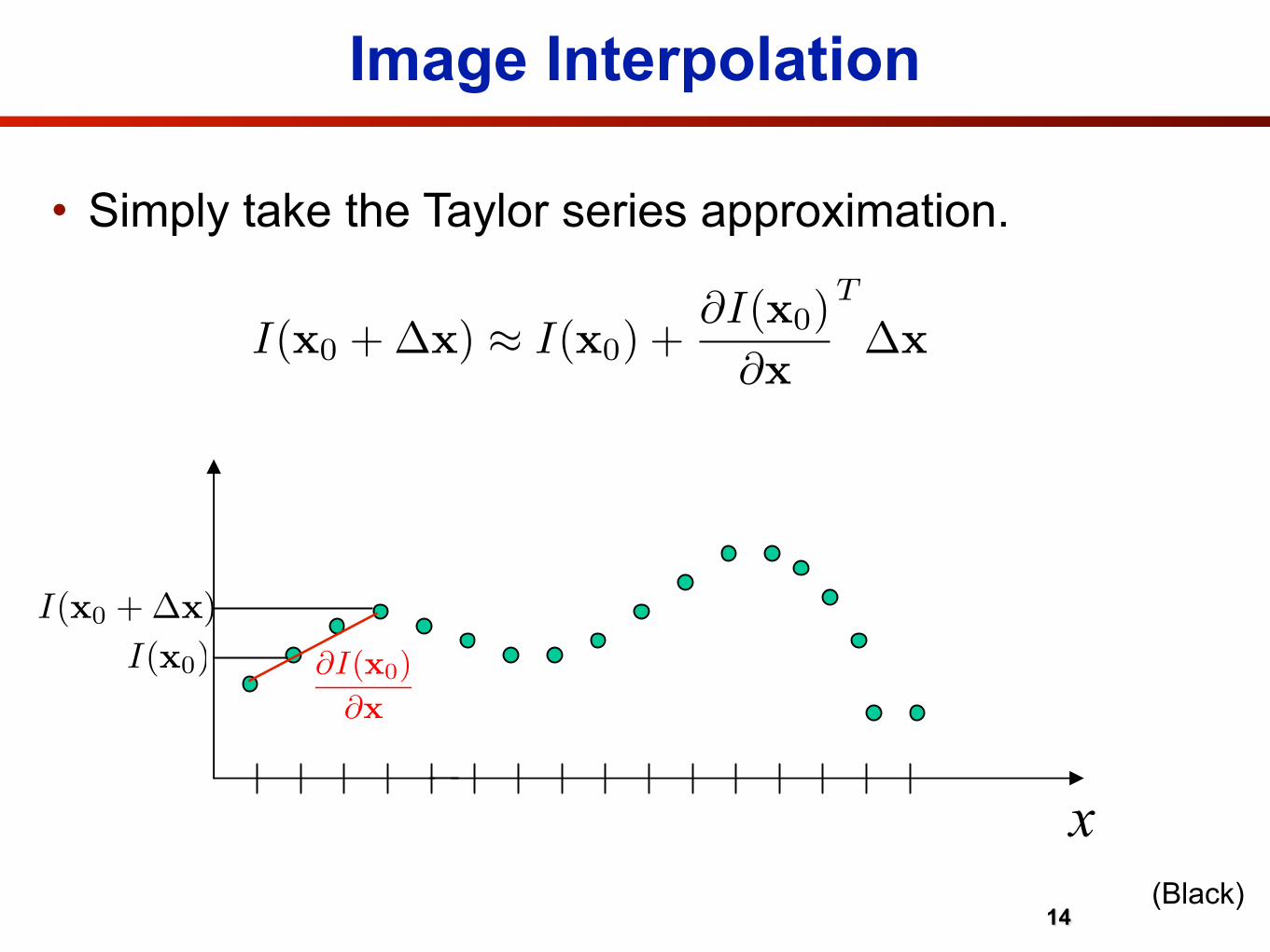
• Simply take the Taylor series approximation.
Image Interpolation
14(Black)
!"#$%&'()*+&)+&!+,-.)/*&0121+("/-)3&4556 7819:;/<&=>&?<;9@
',;A/2&;2&B.(9)1+(2
C ',;A/2&;*/&;&D129*/)/<E&2;,-</D&
*/-*/2/();)1+(&+F&;&9+()1(.+.2&21A(;<
IGxH
x
!"#$%&'()*+&)+&!+,-.)/*&0121+("/-)3&4556 7819:;/<&=>&?<;9@
',;A/2&;2&B.(9)1+(2
C:;)&1D&'&E;()&)+&@(+E&IFx0GdxH&D+*&2,;<<&
dx<#I
IFxH
xx0
I(x0 + �x)I(x0)
I(x0 + �x) � I(x0) +�I(x0)
�x
T
�x
�I(x0)�x

Exhaustive Search
“Images at various warps”

Exhaustive Search
“Images at various warps”“Vectors of pixel values at
each warp position”
[255,134,45,.......,34,12,124,67]
[123,244,12,.......,134,122,24,02]
[67,13,245,.......,112,51,92,181]
[65,09,67,.......,78,66,76,215]
...........

Exhaustive Search
p = {p1, p2}
p1
p 2
“Possible Source Warps”
“Possible Template Warps”
p1
p 2

number of searches! O(nD)
Exhaustive Search
• One can see that as the dimensionality of increases, and, assuming the same number of discrete samples per dimension, the number of searches becomes,
pDn
p (D)Dimensionality of
No.
of s
earc
hes

number of searches! O(nD)
Exhaustive Search
• One can see that as the dimensionality of increases, and, assuming the same number of discrete samples per dimension, the number of searches becomes,
pDn
p (D)Dimensionality of
No.
of s
earc
hes
“Impractical for D >= 3”

Today
• Review - Warp Functions.
• Linearizing Registration.
• Lucas & Kanade Algorithm.

Slightly Less Naive Approach
• Instead of sampling through all possible warp positions to find the best match, let us instead learn a regression,
19
War
p D
ispl
acem
ent
Appearance Displacement

Slightly Less Naive Approach
• Instead of sampling through all possible warp positions to find the best match, let us instead learn a regression,
19
War
p D
ispl
acem
ent
Appearance Displacement
“No longer have to make discrete assumptions about warps.”“Makes warp estimation computationally feasible.”

Problems?
• For us to learn this regression effectively we need to make a couple of assumptions. • What is the distribution of warp displacements? • Is there a relationship between appearance displacement and
warp displacement? • When does this relationship occur, when does it fail?
20
T (0) T (�p)
�p

I(x
,y)
I(x + 1, y + 1)
I
Simoncelli & Olshausen 2001

I(x
,y)
I
I(x + 8, y + 8) Simoncelli & Olshausen 2001

I(x
,y)
I
I(x + 16, y + 16) Simoncelli & Olshausen 2001

I(x
,y)
I
I(x + 50, y + 50) Simoncelli & Olshausen 2001

I(x
,y)
I
I(x + 50, y + 50) Simoncelli & Olshausen 2001

• What if I want to know given that I have only the appearance at and ?I(x0 + �x)
Linearizing Registration
22
(Black)
�x
!"#$%&'()*+&)+&!+,-.)/*&0121+("/-)3&4556 7819:;/<&=>&?<;9@
',;A/2&;2&B.(9)1+(2
C ',;A/2&;*/&;&D129*/)/<E&2;,-</D&
*/-*/2/();)1+(&+F&;&9+()1(.+.2&21A(;<
IGxH
x
!"#$%&'()*+&)+&!+,-.)/*&0121+("/-)3&4556 7819:;/<&=>&?<;9@
',;A/2&;2&B.(9)1+(2
C:;)&1D&'&E;()&)+&@(+E&IFx0GdxH&D+*&2,;<<&
dx<#I
IFxH
xx0
I(x0)
I(x0 + �x)I(x0)

• Again, simply take the Taylor series approximation?
Linearizing Registration
23
(Black)
!"#$%&'()*+&)+&!+,-.)/*&0121+("/-)3&4556 7819:;/<&=>&?<;9@
',;A/2&;2&B.(9)1+(2
C ',;A/2&;*/&;&D129*/)/<E&2;,-</D&
*/-*/2/();)1+(&+F&;&9+()1(.+.2&21A(;<
IGxH
x
!"#$%&'()*+&)+&!+,-.)/*&0121+("/-)3&4556 7819:;/<&=>&?<;9@
',;A/2&;2&B.(9)1+(2
C:;)&1D&'&E;()&)+&@(+E&IFx0GdxH&D+*&2,;<<&
dx<#I
IFxH
xx0
I(x0 + �x)I(x0)
I(x0 +�x) ⇡ I(x0) +@I(x0)
@xT�x

• Again, simply take the Taylor series approximation?
Linearizing Registration
23
(Black)
!"#$%&'()*+&)+&!+,-.)/*&0121+("/-)3&4556 7819:;/<&=>&?<;9@
',;A/2&;2&B.(9)1+(2
C ',;A/2&;*/&;&D129*/)/<E&2;,-</D&
*/-*/2/();)1+(&+F&;&9+()1(.+.2&21A(;<
IGxH
x
!"#$%&'()*+&)+&!+,-.)/*&0121+("/-)3&4556 7819:;/<&=>&?<;9@
',;A/2&;2&B.(9)1+(2
C:;)&1D&'&E;()&)+&@(+E&IFx0GdxH&D+*&2,;<<&
dx<#I
IFxH
xx0
I(x0 + �x)I(x0) �I(x0)
�x
I(x0 +�x) ⇡ I(x0) +@I(x0)
@xT�x
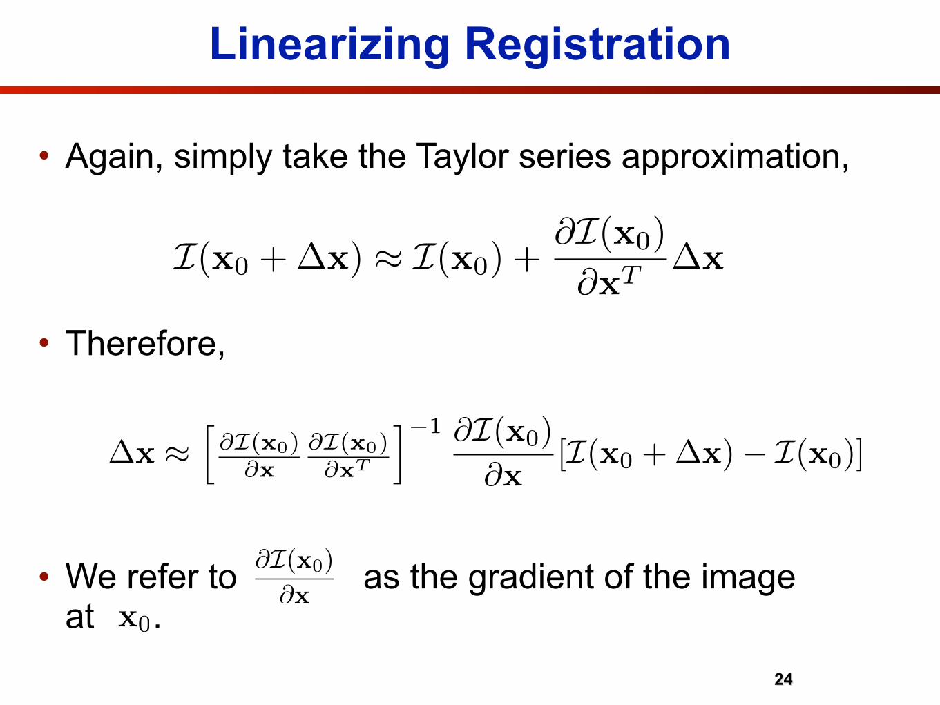
• Again, simply take the Taylor series approximation,
• Therefore,
• We refer to as the gradient of the image at .
Linearizing Registration
24
x0
I(x0 +�x) ⇡ I(x0) +@I(x0)
@xT�x
@I(x0)
@x
�x ⇡h@I(x0)
@x@I(x0)@xT
i�1 @I(x0)
@x[I(x0 +�x)� I(x0)]

• Traditional method for calculating gradients in vision is through the use of edge filters. (e.g., Sobel, Prewitt).
• where,
�
�
Gradients through Filters
25
“Horizontal”
“Vertical”
⇥I(x)⇥x
= [�Ix(x),�Iy(x)]T
�Iy
�Ix
I

• Traditional method for calculating gradients in vision is through the use of edge filters. (e.g., Sobel, Prewitt).
• where,
�
�
Gradients through Filters
25
“Horizontal”
“Vertical”
⇥I(x)⇥x
= [�Ix(x),�Iy(x)]T
�Iy
�Ix
I
“Often have to apply a smoothing filter as well.”

I(x + �x) � I(x) + wTx �x + b
I(x
+�
x)�
I(x)
Gradients through Regression
• Another strategy is to learn a least-squares regression for every pixel in the source image such that,
26
x 2 N

I(x + �x) � I(x) + wTx �x + b
I(x
+�
x)�
I(x)
Gradients through Regression
• Another strategy is to learn a least-squares regression for every pixel in the source image such that,
26
wx
x 2 N
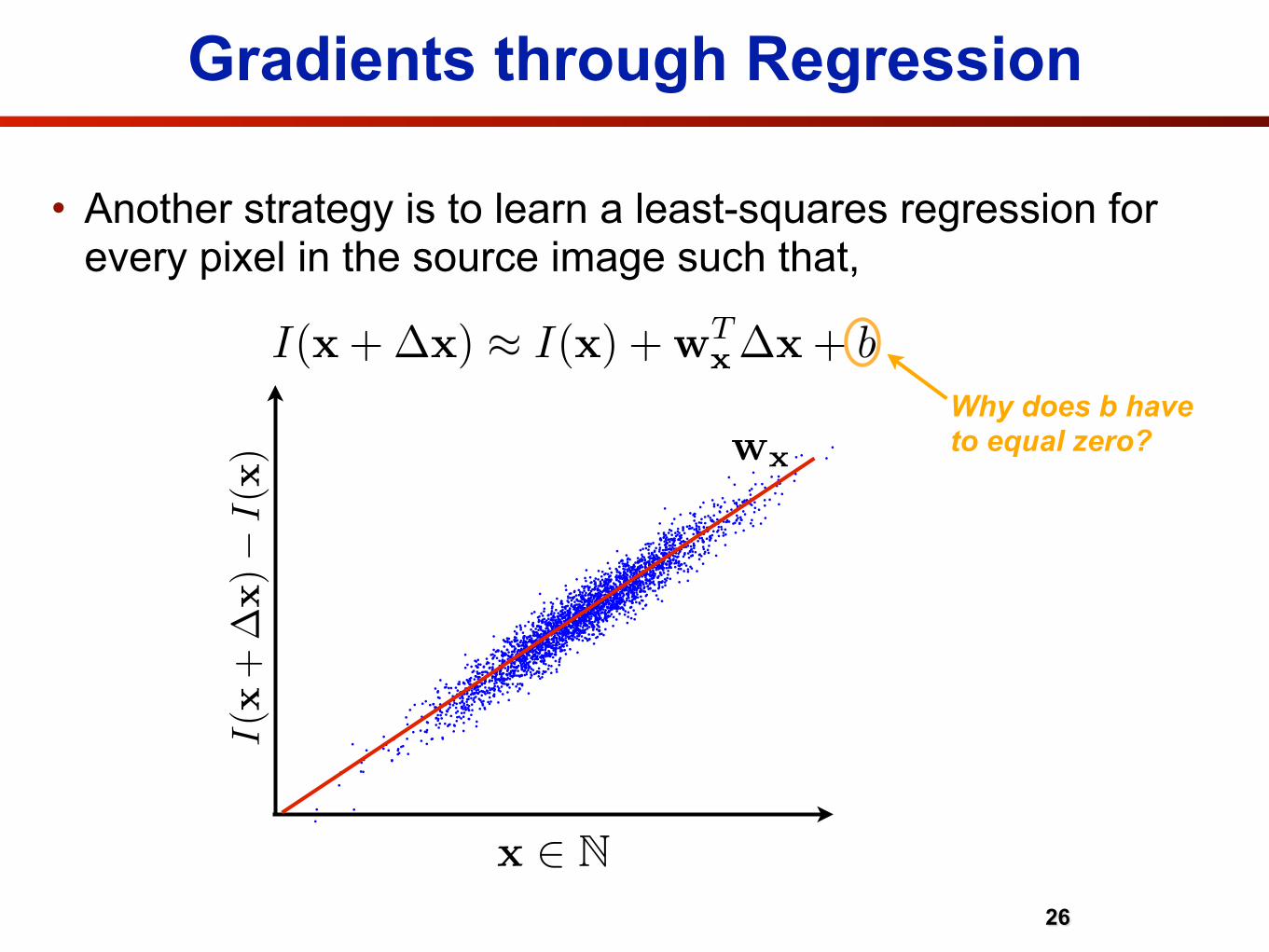
I(x + �x) � I(x) + wTx �x + b
I(x
+�
x)�
I(x)
Gradients through Regression
• Another strategy is to learn a least-squares regression for every pixel in the source image such that,
26
wx
Why does b have to equal zero?
x 2 N

wx =
�⇤
�x⇥N�x�xT
⇥�1 �⇤
�x⇥N�x[I(x + �x)� I(x)]
⇥
Gradients through Regression
• Can be written formally as,
• Solution is given as,
27
arg minwx
�
�x�N||I(x + �x)� I(x)�wT
x �x||2

• Can solve for gradients using least-squares regression. • Has nice properties: expand neighborhood, no heuristics.
• where,
Gradients through Regression
28
�Iy
�Ix
I
Learn Regressor for each
Pixel
⇥I(x)⇥x
= [�Ix(x),�Iy(x)]T = [wx, wy]T

� �p�z =
�
⇧⇤�x1
...�xN
⇥
⌃⌅�
Possible Solution?
• Could we now just solve for individual pixel translation, and then estimate a complex warp from these motions?
29
“Motion Field for Rotation”

CS143 Intro to Computer VisionOct, 2007 ©Michael J. Black
Spatial Coherence
Assumption
* Neighboring points in the scene typically belong to the same
surface and hence typically have similar motions.
* Since they also project to nearby points in the image, we expect
spatial coherence in image flow.
Spatial Coherence
30
• Problem is pixel noise. Individual pixels are too noisy to be reliable estimators of pixel movement (optical flow).
• Fortunately, neighboring points in the scene typically belong to the same surface and hence typically have similar motions .W(x;p)

xi = i-th 2D coordinatep = parametric form of warp
Reminder: Warp Functions• To perform alignment we need a formal way of describing
how the template relates to the source image. • To do this we can employ what is known as a warp function:-
31
W(x;p)
where,
x
x
0

Today
• Review - Warp Functions.
• Linearizing Registration.
• Lucas & Kanade Algorithm.

Lucas & Kanade Algorithm
• Lucas & Kanade (1981) realized this and proposed a method for estimating warp displacement using the principles of gradients and spatial coherence.
• Technique applies Taylor series approximation to any spatially coherent area governed by the warp .
33
W(x;p)
I(p+�p) ⇡ I(p) + @I(p)@pT
�p

Lucas & Kanade Algorithm
• Lucas & Kanade (1981) realized this and proposed a method for estimating warp displacement using the principles of gradients and spatial coherence.
• Technique applies Taylor series approximation to any spatially coherent area governed by the warp .
34
“We consider this image to always be static....”
W(x;p)
I(p+�p) ⇡ I(p) + @I(p)@pT
�p

Lucas & Kanade Algorithm
• Lucas & Kanade (1981) realized this and proposed a method for estimating warp displacement using the principles of gradients and spatial coherence.
• Technique applies Taylor series approximation to any spatially coherent area governed by the warp .
35
W(x;p)
I(p+�p) ⇡ I(p) + @I(p)@pT
�p

Lucas & Kanade Algorithm
• Lucas & Kanade (1981) realized this and proposed a method for estimating warp displacement using the principles of gradients and spatial coherence.
• Technique applies Taylor series approximation to any spatially coherent area governed by the warp .
36
W(x;p)
I(p+�p) ⇡ I(p) + @I(p)@pT
�p
@I(p)@pT
=
2
664
@I(x01)
@x0T1
. . . 0T
.... . .
...
0T . . . @I(x0N )
@x0TN
3
775
2
664
@W(x1;p)@pT
...@W(xN ;p)
@pT
3
775
x
0 = W(x;p)

Lucas & Kanade Algorithm
37
rx
I ryI
@I(p)@pT
=
2
664
@I(x01)
@x0T1
. . . 0T
.... . .
...
0T . . . @I(x0N )
@x0TN
3
775
2
664
@W(x1;p)@pT
...@W(xN ;p)
@pT
3
775

Lucas & Kanade Algorithm
38
@I(p)@pT
=
2
664
@I(x01)
@x0T1
. . . 0T
.... . .
...
0T . . . @I(x0N )
@x0TN
3
775
2
664
@W(x1;p)@pT
...@W(xN ;p)
@pT
3
775
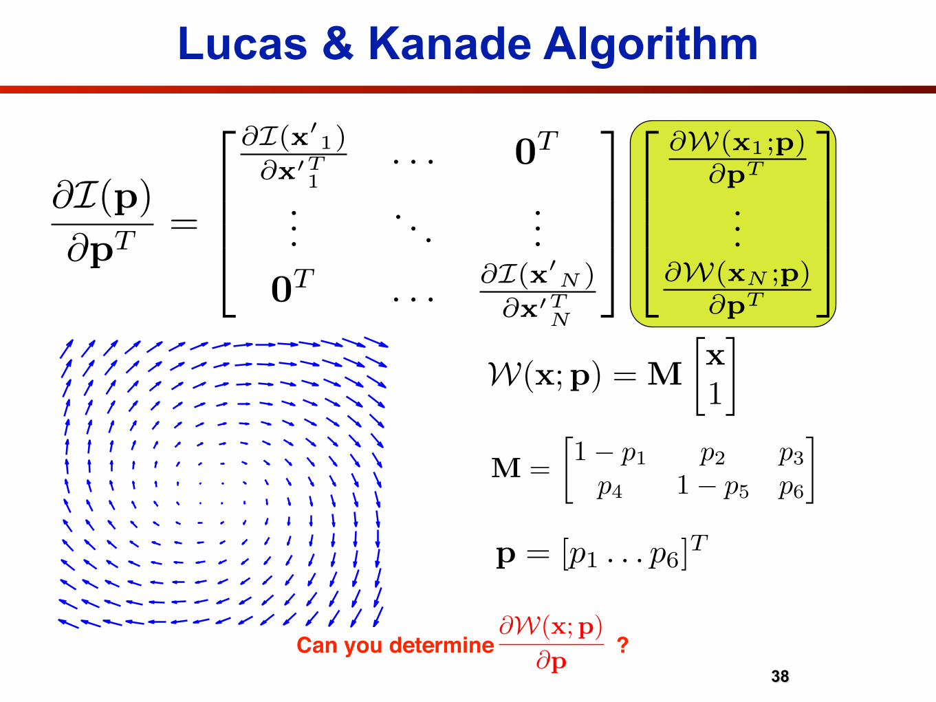
Lucas & Kanade Algorithm
38
W(x;p) = M
x
1
�
p = [p1 . . . p6]T
M =1� p1 p2 p3
p4 1� p5 p6
�
Can you determine ? @W(x;p)
@p
@I(p)@pT
=
2
664
@I(x01)
@x0T1
. . . 0T
.... . .
...
0T . . . @I(x0N )
@x0TN
3
775
2
664
@W(x1;p)@pT
...@W(xN ;p)
@pT
3
775
N � 1
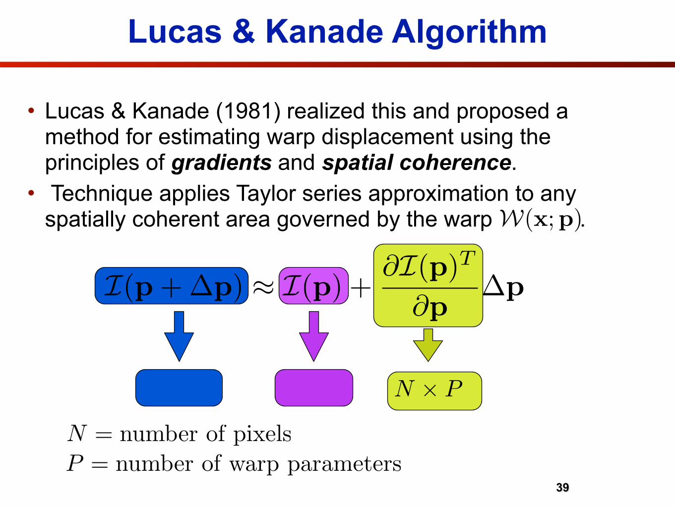
N = number of pixels
Lucas & Kanade Algorithm
• Lucas & Kanade (1981) realized this and proposed a method for estimating warp displacement using the principles of gradients and spatial coherence.
• Technique applies Taylor series approximation to any spatially coherent area governed by the warp .
39
N � 1
I(p+�p) ⇡ I(p) + @I(p)T
@p�p
W(x;p)
P = number of warp parameters
N ⇥ P

• Often just refer to,
as the “Jacobian” matrix. • Also refer to,
as the “pseudo-Hessian”. • Finally, we can refer to,
as the “template”.
Lucas & Kanade Algorithm
40
T (0) = I(p+�p)
JI =@I(p)@pT
HI = JTIJI

• Actual algorithm is just the application of the following steps,
keep applying steps until converges.
Lucas & Kanade Algorithm
41
Step 1:
Step 2:
�p
p� p + �p
�p = H�1I JT
I [T (0)� I(p)]

Examples of LK Alignment
42

Examples of LK Alignment
42
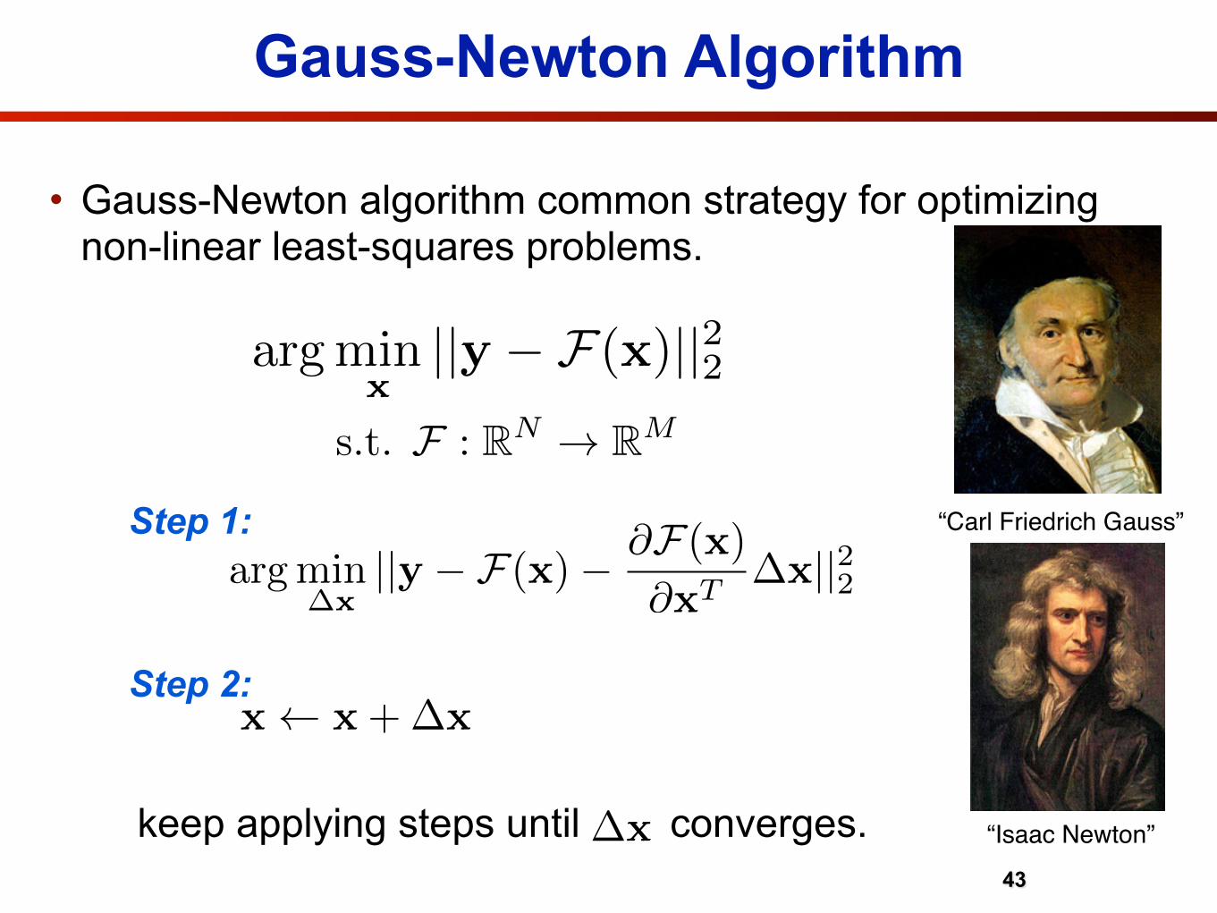
Gauss-Newton Algorithm
• Gauss-Newton algorithm common strategy for optimizing non-linear least-squares problems.
43
s.t. F : RN ! RM
argmin�x
||y � F(x)� @F(x)
@xT�x||22
x x+�x
Step 1:
Step 2:
keep applying steps until converges. �x
argminx
||y � F(x)||22
“Carl Friedrich Gauss”
“Isaac Newton”

Initialization• Initialization has to be suitably close to the ground-truth for
method to work. • Kind of like a black hole’s event horizon. • You got to be inside it to be sucked in!

Gauss-Newton Optimization
Can we approximate the true objective with a convex one?

More to read…
• Lucas & Kanade, “An Iterative Image Registration Technique with Application to Stereo Vision”, IJCAI 1981.
• Baker & Matthews, “Lucas-Kanade 20 Years On: A Unifying Framework”, IJCV 2004.
• Bristow & Lucey, “In Defense of Gradient-Based Alignment on Densely Sampled Sparse Features”, Springer Book on Dense Registration Methods 2015.
In Defense of Gradient-Based Alignment
on Densely Sampled Sparse Features
Hilton Bristow and Simon Lucey
Abstract In this chapter, we explore the surprising result that gradient-based continuous optimization methods perform well for the alignment ofimage/object models when using densely sampled sparse features (HOG,dense SIFT, etc.). Gradient-based approaches for image/object alignmenthave many desirable properties – inference is typically fast and exact, anddiverse constraints can be imposed on the motion of points. However, the pre-sumption that gradients predicted on sparse features would be poor estima-tors of the true descent direction has meant that gradient-based optimizationis often overlooked in favour of graph-based optimization. We show that thisintuition is only partly true: sparse features are indeed poor predictors of theerror surface, but this has no impact on the actual alignment performance.In fact, for general object categories that exhibit large geometric and ap-pearance variation, sparse features are integral to achieving any convergencewhatsoever. How the descent directions are predicted becomes an importantconsideration for these descriptors. We explore a number of strategies forestimating gradients, and show that estimating gradients via regression in amanner that explicitly handles outliers improves alignment performance sub-stantially. To illustrate the general applicability of gradient-based methodsto the alignment of challenging object categories, we perform unsupervisedensemble alignment on a series of non-rigid animal classes from ImageNet.
Hilton BristowQueensland University of Technology, Australia. e-mail: [email protected]
Simon LuceyThe Robotics Institute, Carnegie Mellon University, USA. e-mail: [email protected]
1
![Lucas-Kanade 20 Years On: A Unifying Framework Part 1: The ... · 2 Background: Lucas-Kanade The original image alignment algorithm was the Lucas-Kanade algorithm [13]. The goal of](https://static.fdocuments.net/doc/165x107/5f01f5717e708231d401e04d/lucas-kanade-20-years-on-a-unifying-framework-part-1-the-2-background-lucas-kanade.jpg)

![Lucas-Kanade 20 Years On: A Unifying Framework: Part 4 · Lucas-Kanade 20 Years On: A Unifying Framework: Part 4 Simon Baker, Ralph Gross, and Iain Matthews ... and face coding [10,17].](https://static.fdocuments.net/doc/165x107/5bac70d609d3f2f4158da304/lucas-kanade-20-years-on-a-unifying-framework-part-4-lucas-kanade-20-years.jpg)