The Long-Term Costs of Government Surveillance: Insights ... · SOEPpapers on Multidisciplinary...

SOEPpaperson Multidisciplinary Panel Data Research

The GermanSocio-EconomicPanel study

The Long-Term Costs of Government Surveillance: Insights from Stasi Spying in East Germany

Andreas Lichter, Max Löffl er, Sebastian Siegloch

865 201

6SOEP — The German Socio-Economic Panel study at DIW Berlin 865-2016

SOEPpapers on Multidisciplinary Panel Data Research at DIW Berlin This series presents research findings based either directly on data from the German Socio-Economic Panel study (SOEP) or using SOEP data as part of an internationally comparable data set (e.g. CNEF, ECHP, LIS, LWS, CHER/PACO). SOEP is a truly multidisciplinary household panel study covering a wide range of social and behavioral sciences: economics, sociology, psychology, survey methodology, econometrics and applied statistics, educational science, political science, public health, behavioral genetics, demography, geography, and sport science. The decision to publish a submission in SOEPpapers is made by a board of editors chosen by the DIW Berlin to represent the wide range of disciplines covered by SOEP. There is no external referee process and papers are either accepted or rejected without revision. Papers appear in this series as works in progress and may also appear elsewhere. They often represent preliminary studies and are circulated to encourage discussion. Citation of such a paper should account for its provisional character. A revised version may be requested from the author directly. Any opinions expressed in this series are those of the author(s) and not those of DIW Berlin. Research disseminated by DIW Berlin may include views on public policy issues, but the institute itself takes no institutional policy positions. The SOEPpapers are available at http://www.diw.de/soeppapers Editors: Jan Goebel (Spatial Economics) Martin Kroh (Political Science, Survey Methodology) Carsten Schröder (Public Economics) Jürgen Schupp (Sociology) Conchita D’Ambrosio (Public Economics, DIW Research Fellow) Denis Gerstorf (Psychology, DIW Research Director) Elke Holst (Gender Studies, DIW Research Director) Frauke Kreuter (Survey Methodology, DIW Research Fellow) Frieder R. Lang (Psychology, DIW Research Fellow) Jörg-Peter Schräpler (Survey Methodology, DIW Research Fellow) Thomas Siedler (Empirical Economics) C. Katharina Spieß ( Education and Family Economics) Gert G. Wagner (Social Sciences)

ISSN: 1864-6689 (online)

German Socio-Economic Panel (SOEP) DIW Berlin Mohrenstrasse 58 10117 Berlin, Germany Contact: Uta Rahmann | [email protected]

The Long-Term Costs of Government Surveillance:Insights from Stasi Spying in East Germany∗

Andreas Lichter Max Loffler Sebastian Siegloch

Version: August 2016

Abstract. Despite the prevalence of government surveillance systems around the world,causal evidence on their social and economic consequences is lacking. Using county-levelvariation in the number of Stasi informers within Socialist East Germany during the 1980sand accounting for potential endogeneity, we show that more intense regional surveillanceled to lower levels of trust and reduced social activity in post-reunification Germany. Wealso find substantial and long-lasting economic effects of Stasi spying, resulting in lowerself-employment, higher unemployment and larger out-migration throughout the 1990sand 2000s. We further show that these effects are due to surveillance and not alternativemechanisms. We argue that our findings have important implications for contemporarysurveillance systems.

Keywords: government surveillance, trust, social ties, East GermanyJEL codes: H11, N34, N44, P20

* A. Lichter is affiliated to the Institute for the Study of Labor (IZA) and the University of Cologne ([email protected]),M. Loffler to the Centre for European Economic Research (ZEW) and the University of Cologne ([email protected]),S. Siegloch to the University of Mannheim, IZA, ZEW and CESifo ([email protected]). A first version of thispaper circulates as IZA Discussion Paper No. 9245 (July 2015). We are grateful to Jens Gieseke for sharing county-leveldata on official employees of the Ministry for State Security, and Davide Cantoni for sharing regional GDR data withus. We thank Felix Bierbrauer, Davide Cantoni, Antonio Ciccone, Arnaud Chevalier, Denvil Duncan, Corrado Giulietti,Mark Harrison, Johannes Hermle, Paul Hufe, Michael Krause, Andreas Peichl, Gerard Pfann, Martin Peitz, NicoPestel, Anna Raute, Derek Stemple, Jochen Streb, Uwe Sunde, Nico Voigtlander, Fabian Waldinger, Felix Weinhardt,Ludger Woßmann as well as conference participants at IIPF 2015, SOLE 2016, and seminar participants at IZA Bonn,ZEW Mannheim, BeNA Berlin, and the Universities of Mannheim, Munster and Bonn for valuable comments andsuggestions. Felix Poge and Georgios Tassoukis provided outstanding research assistance. We would also like to thankthe SOEPremote team at DIW Berlin for continuous support.

1

mailto:[email protected]



1 Introduction

More than one third of the world population lives in authoritarian states that attempt to controlalmost all aspects of public and private life (The Economist Intelligence Unit, 2014). To these ends,those regimes install large-scale surveillance systems that infiltrate the population and generatea widespread atmosphere of suspicion reaching deep into private spheres (Arendt, 1951). Suchenvironments of distrust are thought to have adverse economic effects, since they limit cooperationand the open exchange of ideas (Arrow, 1972, Putnam, 1995, La Porta et al., 1997, Algan and Cahuc,2014). However, the empirical literature has not yet established a causal link between governmentsurveillance, trust and economic performance.

In this paper, we quantify the effect of government surveillance on trust, social ties and long-run economic performance. To do so, we make use of administrative data on the large networkof informers who once operated in the socialist German Democratic Republic (GDR) and linkmeasures of regional government surveillance to post-reunification outcomes. The GDR Ministry forState Security, commonly referred to as the Stasi, administered a huge body of so-called InformelleMitarbeiter – unofficial informers – that accounted for more than one percent of the East Germanpopulation in the 1980s. The regime actually regarded its dense network of informers as the mostimportant instrument to secure its power (Muller-Enbergs, 1996, p. 305). The informers were ordinarycitizens who kept their regular jobs but also secretly gathered information within their professionaland social network, thus betraying the trust of friends, neighbors and colleagues (Bruce, 2010). Asthe informers infiltrated private spheres, the damage done to social relations is thought to be largeand persistent (Gieseke, 2014, p. 95).

To identify the long-term effects of surveillance, we exploit regional variation in the spying densityacross East German counties. An obvious concern is that the recruitment of spies across countieswas non-random. We account for this non-randomness by adopting two different, complementaryidentification strategies. The first design exploits the specific administrative structure of the Stasi,whose county offices were subordinate to the respective state office. These state offices bore fullresponsibility to secure their territory and chose different strategies to do so, which led to differentaverage levels of spying across states. Indeed, around 25% of the variation in the surveillance intensityacross counties can be explained with state fixed effects. However, while surveillance policies variedacross states, all economic and social policies were centrally decided by the politburo in East Berlin.This allows us to follow Dube et al. (2010) and use the discontinuities along state borders as a sourceof exogenous variation. For our second identification strategy, we follow Moser et al. (2014) andconstruct a county-level panel dataset covering both pre- and post-treatment years. This researchdesign enables us to include county fixed effects to account for time-invariant confounders, sayregional liberalism, that might have affected the recruitment of Stasi spies and may (still) haveeconomic effects. Using pre-treatment data from the 1920s and early 1930s, we can also test forpre-trends in the outcome variables. Reassuringly, spying density cannot explain trends in economicperformance prior to the division of Germany, which strengthens the causal interpretation of ourfindings.

Overall, the results of our study offer substantial evidence for negative and long-lasting effects

2

of government surveillance on peoples’ trust, social ties and economic performance.1 Using datafrom the German Socio-Economic Panel (SOEP), we find that a higher spying density leads to lowertrust in strangers and stronger negative reciprocity. Both measures have been used as proxies forinterpersonal trust in the literature (Glaeser et al., 2000, Dohmen et al., 2009). Individuals in countieswith greater spying density also rate themselves as less sociable. These differences in beliefs andself-assessment are also reflected in individual social behavior, as we show the number of closefriends to be significantly lower in counties with higher levels of surveillance. Moreover, individualsin counties with a higher informer density volunteer less frequently in associations, clubs or socialservices and are less engaged in local politics; both outcomes serving as common measures of socialcapital (Putnam, 2000, Satyanath et al., 2016). Hence, a higher density of informers among thepopulation resulted in the undermining of trust, a withdrawal from society and an erosion of socialcapital.

The negative and persistent effect of a greater spying density on trust and social interactionsis accompanied by negative and persistent effects on various measures of economic performance.Individual labor income and county-level self-employment rates are lower in counties with historicallygreater spying densities, while unemployment rates are higher. The effects are sizable. For example,our estimates imply that moving from the 75th to the 25th percentile in the intensity of surveillancewould lower the long-term unemployment rate by 0.84 percentage points, which is equivalent to a4.5 percent drop. We also document that the GDR surveillance system was a significant driver of thetremendous out-migration experienced in East Germany after reunification.

Our empirical results are robust to a number of sensitivity checks. First, we demonstrate theimportance of accounting for the non-randomness of informer recruitment. The magnitudes ofour estimates increase both when applying the border discontinuity design and controlling forhistorical confounders. This suggests that the endogeneity of the informer density biases estimatestowards zero. Furthermore, we provide evidence that our effects are indeed driven by differencesin the intensity of surveillance and are neither caused by local variation in socialist indoctrinationnor by differences in government transfers and subsidies that were paid to East German countiesafter reunification in order to rebuild public infrastructure. We further test whether second-roundmigration and/or income effects drive our results, finding no evidence of such indirect effects.Moreover, we show that our results are not due to selective out-migration in terms of skills and age.

This is the first study to show that government surveillance has a causal negative effect on economicperformance. We study the case of socialist East Germany, but our findings also have importantimplications with regard to contemporary forms of mass surveillance in authoritarian states. Whilewe fully acknowledge the differences in the specifics and intensities of surveillance programs acrossregimes and time, a common feature of such programs is to exploit social networks to gatherinformation (Arendt, 1951). In fact, the intrusion into private spheres was already present in Romantimes when the politician and orator Cicero feared that his private letters were intercepted by therulers (Zurcher, 2013). Given this common denominator, it is likely that contemporary government

1 The annual number of requests for disclosure of information on Stasi activity (Burgerantrage) serves as a first indicationthat East German citizens are still affected by Stasi spying, even 25 years after the fall of the Iron Curtain. FigureA.1 in the Appendix plots the annual number of requests filed from 1992–2012. Unfortunately, there is no regionalinformation on these requests, which could provide an interesting outcome for our analysis.

3

surveillance in authoritarian states such as China or Russia exerts similar negative effects on socialinteractions and economic performance.2

Our results also relate to recent developments in surveillance strategies of democratic countries,where the threat of global terrorism and political extremism has led to the implementation of large-scale surveillance programs in recent years. Optimal policy needs to balance benefits of surveillance,i.e., security, with its costs. However, the potential costs, such as the violation of human privacyrights, social repression and the undermining of sociability and trust (Haggerty and Samatas, 2010,Anderson, 2016), are rather intangible and difficult to measure. Our study (i) demonstrates thatthese social costs exist, (ii) shows that they are sizable and (iii) points to additional economic costsassociated with the reduction in social interactions. Importantly, these effects seem to be independentof the surveillance technology.3 There is, for instance, ample anecdotal evidence that the revelationof the NSA secrets affected ordinary peoples’ trust in the government (see, e.g., Schneier, 2013).Moreover, a substantial share of people stated that they adjusted their use of telecommunication as aconsequence of the Snowden affair (Pew Research Center, 2014).

Our study is closely linked to the steadily growing literature on culture, institutions and economicperformance (see Alesina and Giuliano, 2015, for a recent survey). In particular, we complementthe large literature providing (mostly cross-country) evidence on the long-term positive effects ofinstitutional quality on economic performance (Mauro, 1995, Hall and Jones, 1999, Rodrik et al., 2004,Nunn, 2008, Tabellini, 2010, Nunn and Wantchekon, 2011, Acemoglu et al., 2015). Econometrically,we refine current identification strategies to estimate causal effects of formal institutions on cultureand economic outcomes by combining regional, within-country variation (Tabellini, 2010, Alesinaet al., 2013) with spatial discontinuity designs (Becker et al., 2016, Fontana et al., 2016). In contrastto other studies, our identifying variation is not generated by deep, historical differences such asreligion, ethnicity, or education, but induced by a rather recent, pervasive political experiment.

Our paper also speaks to the literature on trust, social capital and economic performance (see, e.g.,Algan and Cahuc, 2014, Fuchs-Schundeln and Hassan, 2015, for recent surveys). Specifically, wehighlight the importance of trust and social ties for economic prosperity (Knack and Keefer, 1997,Zak and Knack, 2001, Guiso et al., 2006, Algan and Cahuc, 2010, Burchardi and Hassan, 2013, Butleret al., 2016). In line with La Porta et al. (1997), our findings point to reduced entrepreneurial activityas an important channel for the economic decline. Given the intergenerational transmission of trustand reciprocity (Nunn and Wantchekon, 2011, Dohmen et al., 2012), it is likely that the East Germansurveillance regime will lead to a long-lasting deterioration of trust and social interactions.

Last, we contribute to the literature investigating the transformation of former countries of theEastern bloc after the fall of the Iron Curtain (see, e.g., Shleifer, 1997). For the German case, wecomplement the evidence provided by Alesina and Fuchs-Schundeln (2007) and show that the East

2 In China, the government tries to demobilize protesters by inducing pressure via the critics’ social network (Deng andO’Brien, 2013). Various accounts further demonstrate that the one-party state still heavily relies on a large networkof informers (see, e.g., Branigan, 2010, Jacobs and Ansfield, 2011, Yu, 2014). Likewise, Russia has been observed tore-implement surveillance strategies, in which secret informers and denunciations play an important role to controloppositional forces (Capon, 2015).

3 While technological progress has enabled governments to intercept a substantial share of the personal communicationelectronically, informants still constitute an important element of the surveillance strategy. Consider, for instance,Stabile (2014) for a discussion of legal problems associated with the FBI informant recruitment, or the current case ofthe Orlando shooting (Lichtbaum and Apuzzo, 2016).

4

German regime not only affected individual preferences for redistribution, but also had long-lastingeffects on trust and social behavior. In contrast to Alesina and Fuchs-Schundeln (2007), we exploitvariation within East Germany rather than estimating the total effect of being exposed to the socialistregime by comparing East and West German individuals. There are two related papers, which alsoexploit the number of informers to identify post-reunification effects.4 However, both papers do notaccount for the potential non-randomness in the regional spying density.5 The first one by Jacoband Tyrell (2010) looks at the impact of surveillance on social capital, the second one focuses onpersonality traits (Friehe et al., 2015). Moreover, our paper also investigates long-run economic effects.Our negative estimates complement recent findings by Fuchs-Schundeln and Masella (2016), whoshow long-run negative effects of socialist education on labor market outcomes.

The remainder of this paper is organized as follows. Section 2 presents the historical backgroundand the institutional framework of the Stasi. Section 3 describes the data, while Section 4 investigatespotential determinants of the informer density across counties. Section 5 introduces our researchdesign and explains the two different identification strategies. Results are presented in Section 6,before Section 7 concludes.

2 Historical background

After the end of World War II and Germany’s liberation from the Nazi regime in 1945, the remainingGerman territory was occupied by and divided among the four Allied forces – the US, the UK,France and the Soviet Union. The boundaries between these zones were drawn along the territorialboundaries of 19th-century German states and provinces that were “economically well-integrated”(Wolf, 2009, p. 877) when the Nazis gained power. On July 1, 1945, roughly two months after the totaland unconditional surrender of Germany, the division into the four zones became effective. With theSoviet Union and the Western allies disagreeing over Germany’s political and economic future, theborders of the Soviet occupation zone soon became the official inner-German border and eventuallyled to a 40-year long division of the society. In May 1949, the Federal Republic of Germany wasestablished in the three western occupation zones. Only five months later, the German DemocraticRepublic, a state in the spirit of “real socialism”6 and a founding member state of the Warsaw Pact,was constituted in the Soviet ruled zone. Until the sudden and unexpected fall of the Berlin Wallon the evening of November 9, 1989 and the reunification of West and East Germany in October1990, the GDR was an authoritarian regime under the rule of the Socialist Unity Party (SED) and itssecretaries general.

In February 1950, just a few months after the constitution of the GDR, the Ministry for StateSecurity was founded. The Stasi served as the internal (and external) intelligence agency of thesocialist regime and was designed to “battle against agents, saboteurs, and diversionists [in order] to

4 In addition, Glitz and Meyersson (2016) exploit information provided by East German foreign intelligence spies in theWest to investigate the economic returns to industrial espionage.

5 We show below that simple OLS estimates are upward biased. For instance, the correlation between trust – the mostfrequently used measure of social capital – and the spying density across counties turns out to be positive.

6 Erich Honecker, Secretary General of the Socialist Unity Party between 1971–1989, introduced this term on a meeting ofthe Central Committee in May 1973 to distinguish the regimes of the Eastern bloc from Marxist theories on socialism.

5

preserve the full effectiveness of [the] Constitution.”7 After the unforeseen national uprising on andaround June 17, 1953 had revealed the weakness of the secret security service in its infant years, theStasi remarkably expanded its activities and soon turned into a ubiquitous institution, spying on andsuppressing the entire population to ensure and preserve the regime’s power (Gieseke, 2014, p. 50ff.).The key feature of the Stasi’s surveillance strategy was the use of “silent” methods of repressionrather than legal persecution by the police (Knabe, 1999). To these ends, the Stasi administered adense network of unofficial informers, the regime’s ”main weapon against the enemy”8, who secretlygathered detailed inside knowledge about the population. In the 1980s, the Stasi listed around 85,000regular employees and 175,000 unofficial informers, which accounted for around 0.5 and 1.05 percentof the population, respectively.9 With the collected intelligence at hand, the Stasi was able to draw adetailed picture of anti-socialist and dissident movements within the society and to exert an overall”disciplinary and intimidating effect” on the population (Gieseke, 2014, p. 84f.).

In order to extract information from the population, the Stasi relied on a highly decentralizedadministrative structure, which was at odds with the overall centralist organization of the GDR.While the main administration was located in East Berlin, the Stasi maintained state offices (Bezirks-dienststellen) in each capital of the fifteen states, regional offices (Kreisdienststellen) in most of the226 counties and offices in seven Objects of Special Interest, which were large and strategicallyimportant public companies or universities (Objektdienststellen).10 State offices bore full responsibilityto secure their territory and had authority over their subordinate offices in the respective counties.As a consequence, surveillance strategies differed in their intensities across GDR states. For instance,around one-third of the constantly-monitored citizens (Personen in standiger Uberwachung) were livingin the state of Karl-Marx-Stadt (Horsch, 1997), which accounted for only 11 percent of the totalpopulation. Likewise, the state of Magdeburg accounted for 17 percent of the two million buggedtelephone conversations, while this state only accounted for eight percent of the total GDR populationin turn. We exploit this variation in surveillance intensities across states for identification (see Section5.1).

The majority of informers were recruited by the regional offices and instructed to secretly collectinformation about individuals in their own network. Hence, it was necessary that informerspursued their normal lives, being friends, colleagues and neighbors, after recruitment. The Stasiadministrated the body of informers in a highly formalized way, with cooperation being sealed inwritten agreements and informers being tightly led by a responsible Stasi officer (Gieseke, 2014,p. 114ff.). Informers would regularly and secretly meet with their officer, report suspicious behaviorand provide personal information about individuals in their social networks. Reasons for serving asa collaborator were diverse. Some citizens agreed to cooperate due to ideological reasons, otherswere attracted by personal and material benefits accompanied with their cooperation. However, the

7 According to Erich Mielke, subsequent Minister for State Security from 1957 to 1989, on January 28, 1950 in the officialSED party newspaper Neues Deutschland as quoted in Gieseke (2014, p. 12).

8 Directive 1/79 of the Ministry for State Security for the work with unofficial collaborators (Muller-Enbergs, 1996, p. 305).9 The number of regular Stasi employees was notably high when being compared to the size of other secret services in the

Eastern Bloc (Gieseke, 2014, p. 72). While figures on the number of spies in other communist countries entail elementsof uncertainty, other studies suggest that the level of spies in the GDR was at least as high as in other countries of theEastern bloc in the years preceding the fall of the Iron Curtain (Albats, 1995, Harrison and Zaksauskiene, 2015).

10 The Stasi only monitored economic activity but was not actively involved in economic production (Gieseke, 2014).

6

regime also urged citizens to act as unofficial informers by creating fear and pressure. In a 1967survey of unofficial informers, 23 percent of the collaborators indicated that pressure and coercionled to recruitment (Muller-Enbergs, 2013, p. 120).

The threat of being denunciated caused an atmosphere of mistrust and suspicion within a deeplytorn society (Wolle, 2009). Citizens felt the Stasi’s presence like a “scratching t-shirt” (Reich, 1997,p. 28).11 The constant surveillance had perceivable real-life consequences, ranging from studentsbeing denied the opportunity to study at the university, or teachers and factory workers beingdismissed (Bruce, 2010, p. 103f.) to more serious ramifications like physical violence, abuse andsometimes even imprisonment.

3 Data

In this section, we briefly describe the various data sources collected for our empirical analysis.Section 3.1 presents information on our explanatory variable, the spying density in a county. Section3.2 and Section 3.3 describe the data used to construct outcome measures and control variables.Detailed information on all variables are provided in Appendix Table B.1. The Data Appendix B alsoprovides details on the harmonization of territorial county borders over time.

3.1 Stasi data

Information on the number of unofficial informers in each county is based on official Stasi records,published by the Agency of the Federal Commissioner for the Stasi Records and compiled inMuller-Enbergs (2008). Although the Stasi was able to destroy part of its files in late 1989, muchinformation was preserved when protesters started to occupy Stasi offices across the country. Inaddition, numerous shredded files could be restored after reunification. Since 1991, individual Stasirecords have been available for personal inspection as well as requests from researchers and themedia.

Measuring surveillance intensity. Given that the Stasi saw unofficial collaborators as their maininstrument of surveillance, we choose the county-level share of informers in the population as ourpreferred measure of the intensity of surveillance. Most regular Stasi officers were based in theheadquarters in Berlin, and only 10-12 percent of them were employed at the county level. In contrast,the majority of all unofficial collaborators was attached to county offices. The Stasi differentiatedbetween three categories of informers: (1) collaborators for political-operative penetration, homelanddefense, or special operations as well as leading informers, (2) collaborators providing logisticsand (3) societal collaborators, i.e., individuals publicly known as loyal to the state. We use the firstcategory of unofficial collaborators (operative collaborators) to construct our measure of surveillancedensity, as those were actively involved in spying and are by far the largest and most relevantgroup of collaborators. If an Object of Special Interest with a separate Stasi office was located in a

11 For more popular documentations on the impact of the Stasi, see the Academy Award winning movie “The Livesof Others” and the recent TED talk “The dark secrets of a surveillance state” given by the director of the Berlin-Hohenschonhausen Stasi prison memorial, Hubertus Knabe.

7

https://www.ted.com/talks/hubertus_knabe_the_dark_secrets_of_a_surveillance_state

county, we add the number of unofficial collaborators attached to these object offices to the respectivecounty’s number of spies.12 As information on the total number of collaborators are not given foreach year in every county, we use the average share of informers from 1980 to 1988 as our measureof surveillance.13 The spying density in a county was very stable across the 1980s, the within-countycorrelation being 0.91. For further details on our main explanatory variable, see Data Appendix B.

Variation in surveillance intensity. Figure 1 plots the spying density for each county. Today, thenumber of informers is known for about 90 percent of the counties for at least one year in the 1980s.The density of spies differs considerably both across and within GDR states, with the fraction ofunofficial collaborators in the population ranging from 0.12 to 1.03 percent and the mean densitybeing 0.38 percent (see Table A.2 for more detailed distributional information).14 The median issimilar to the mean (0.36 percent), and one standard deviation is equal to 0.14 informers per capita,which is more than one third of the mean spying density. In our regressions, we standardize theshare of informers by dividing it by one standard deviation.

In order to identify the effects of state surveillance on trust and economic performance in thepresent setting, it is crucial that existing differences in the intensity of surveillance across EastGermany significantly affected the population. Historical accounts suggest that the transmissionoccurred both consciously and unconsciously. Bruce (2010, p. 146) documents that the East Germanpopulation was aware of the large number of informants at work, at restaurants, and in public places.Moreover, a large share of the population “had encountered the Stasi at one point or another in theirlives, but these experiences varied greatly” (Bruce, 2010, p. 148). Given the substantial variation inthe spying density, our identifying assumption is that individuals living in counties with a higherinformer density were consciously or subconsciously more aware of government surveillance becausethey had more frequent/intense contact with the surveillance system.

Alternative measures of surveillance intensity. As discussed in Section 2, silent surveillance mea-sures seem more appropriate to capture the repressive nature of the regime, given that the Stasi’smain strategy was to scare regime opponents into terminating their activities (Bruce, 2010, p. 130).Among these silent measures, we choose the number of operative collaborators (category 1) percapita as our main regressor given their active role in spying. Moreover, data coverage is highestfor this type of informant and we would lose 30 counties when basing our measure of surveillanceon all three types of informers. However, as indicated by Panel A of Figure A.2 in the Appendix,this choice does not appear to be crucial as implied by the very high correlation between operativeinformers and the total number of collaborators (ρ = 0.95).

Although most official Stasi employees were based in East Berlin, the number of county officersconstitutes another alternative measure of the regional intensity of surveillance. As before, Panel Bof Figure A.2, however, shows that the number of regular employees and operative collaborators ishighly correlated, which seems reasonable given that informers had to be administered by official

12 In the empirical analysis, we explicitly control for the presence of such offices in Objects of Special Interest.13 Data from earlier years are only available for a limited number of counties.14 Note that these figures only relate to operative collaborators at the county level (informer category 1), which explains

the lower mean in the spying density compared to the overall share of informers in the population (cf. Section 2).

8

Figure 1: Share of Operative Unofficial Informers at the County Level

(.77,1.03](.56,.77](.46,.56](.4,.46](.35,.4](.3,.35](.26,.3](.22,.26](.13,.22][.12,.13]No data

Notes: This graph plots the county-level surveillance density measured by the average yearlyshare of operative unofficial informers relative to the population between 1980 and 1988.Thick black lines show the borders of the fifteen GDR states. White areas indicate missingdata. Map: MPIDR and CGG, 2011.

employees in the respective county offices. Given the importance of unofficial informants as “themain weapon” of the Stasi, we choose the density of operative informers as our baseline explanatoryvariable. We find slightly smaller, but qualitatively similar effects when using the share of regularofficers instead. Taking the total number of informers does not affect our results.

9

3.2 Individual-level data

For the empirical analysis presented below, we rely on two distinct datasets to estimate the effects ofstate surveillance on trust and economic performance. First, we use information from the GermanSocio-Economic Panel Study (SOEP), a longitudinal survey of German households (Wagner et al.,2007).15 Established for West Germany in 1984, the survey covers respondents from the former GDRsince June 1990. The SOEP contains information on the county of residence and when individualshave moved to their current home. We identify and select respondents living in East German countiesin 1990 who have not changed residence in 1989 or 1990.16 We then follow these individuals fromthe 1990 wave of the SOEP over time. By exploiting a variety of different waves of the survey, we areable to observe various measures of trust and social relations as well as current gross labor income(see Section 5.1 and Data Appendix B).

In order to proxy trust, we use two standard measures provided in the SOEP: trust in strangers asspecified in Glaeser et al. (2000), and the negative reciprocity index proposed by Dohmen et al. (2009).To capture individual social behavior, we focus on the number of close friends and self-assessedsociability, the latter being one of the three components of the Big Five personality trait Extraversion.Last, we measure societal engagement by individuals’ volunteering in clubs or social services andby their engagement in local politics. We also use monthly gross labor income out of regularemployment reported in the SOEP as an individual-level measure of economic performance.

Moreover, we rely on the rich survey information to construct a set of individual control variables:gender, age, household size, marital status, level of education and learned profession. Summarystatistics are presented in Table A.1; for information on the underlying survey questions, data yearsand exact variable definitions, see Data Appendix B.

3.3 County-level data

For the second dataset, we compiled county-level data on various measures of economic performance(self-employment, unemployment, population). We collected county-level data for two time-periods,data from the 1990s and 2000s as well as pre World War II data.17 Both post-reunification data andhistorical data come from official administrative records (see Data Appendix B for details).

We further collect various county-level variables as controls. We use these to (i) explain differencesin the Stasi density (cf. Section 4), and (ii) as control variables to check the sensitivity of our estimates.In total, we construct four sets of county-control variables. The first set of variables accounts for thesize and demographic composition of the counties in the 1980s. Therefore, we collect information on themean county population in the 1980s and the area of each county. Moreover, we use information oncounties’ demographic composition as of September 30, 1989 to construct variables indicating theshare of children (population aged below 15) and the share of retirees (population aged above 64) ineach county.

15 Precisely, we use Socio-Economic Panel (SOEP), data for years 1984-2012, version 29, SOEP, 2013, doi: 10.5684/soep.v29.16 As discussed below, residential mobility within the GDR was highly restricted.17 Unfortunately, there are no annual county-level data for self-employment and unemployment for post-reunification East

Germany in the years from 1990 to 1995. We filed several data requests to the various federal and state statistical officesand were informed that the information is simply not available due to the federal structure of the German statisticaloffice system paired with the turbulences following reunification.

10

The second set measures the strength of the opposition to the regime. As mentioned in Section 2,the national uprising on and around June 17, 1953 constituted the most prominent rebellion againstthe regime before the large demonstrations in late 1989. The riot markedly changed the regime’sawareness for internal conflicts and triggered the expansion of the Stasi informer network. We usedifferences in the regional intensity of the riot to proxy the strength of the opposition. Specifically,we construct three control variables: (i) an ordinal measure of the strike intensity with values “none”,“strike”, “demonstration”, “riot”, and “liberation of prisoners”, (ii) a dummy variable indicatingwhether the regime declared a state of emergency in the county and (iii) a dummy equal to one ifthe Soviet military intervened in the county.

The third set of controls takes into account county differences in the industry composition. Ourset of industry controls comprise (i) the 1989 share of employees in the industrial sector and theshare in the agricultural sector, (ii) the goods value of industrial production in 1989 (in logs)18,(iii) a dummy variable indicating whether a large enterprise from the uranium, coal, potash, oilor chemical industry was located in the county, and (iv) a measure of the relative importance ofone specific industrial sector for overall industrial employment (i.e., the 1989 share of employeesin a county’s dominant industry sector over all industrial employees). This measure is intended toaddress potential concerns that important industries dominated certain regions during the GDRregime but then became unimportant after reunification.

The fourth set of controls is intended to pick up historical and potentially persistent countydifferences in terms of economic performance and political ideology. It will be used in the modelson the individual level in the absence of pre-treatment information on the outcomes. Our pre WorldWar II controls include (i) the mean Nazi and Communist vote shares in the federal elections of1928, 1930 and the two 1932 elections to capture political extremism (Voigtlander and Voth, 2012),(ii) average electoral turnout in the same elections to proxy institutional trust, (iii) the regional shareof protestants in 1925 in order to control for differences in work ethic and/or education (Becker andWoßmann, 2009), (iv) the share of self-employed in 1933 to capture regional entrepreneurial spirit and(v) the unemployment rate in 1933 to capture pre-treatment differences in economic performance.

Summary statistics for all county-level variables are presented in Table A.2; for information on thesources, data years and exact variable definitions, see Data Appendix B.

4 Explaining the informer density

In this section, we try to explain county differences in the informer density. Astonishingly, thereis very little knowledge regarding the determinants of regional spying density. Some anecdotalevidence suggests that the Stasi was particularly active in regions with strategically importantindustry clusters. In contrast and somewhat surprisingly, previous historical research could notestablish a clear correlation between the density of spying and the size of the opposition at thecounty level (Gieseke, 1995, p. 190). In order to shed some light on the determinants of the regionalsurveillance intensity, we run simple OLS regressions of the spying density on five sets of potentiallyimportant variables: (i) county size and demographic structure, (ii) county-level oppositional strength,

18 We drop the county Plauen-Land due to missing data for this variable.

11

(iii) county industry composition, (iv) county-level pre World War II characteristics, and (v) GDRstate-level characteristics (control sets are defined as above, see Section 3.3). We check the importanceof each set of controls in explaining the county-level variation in the spying intensity as indicated by(partial) R2 measures.

Table 1 reports the regression results. We start off by explaining the spying density with a constantand a dummy variable, which is equal to one if one of the seven offices in Objects of Special Interest,that is, an institution (company or university) of strategic importance, was located in the county.19

In the next specification, we add variables controlling for the size and demographic structure of acounty. While the spying density already accounts for differences in county population, we add thelog mean county population in the 1980s and the log square meter area of the county as regressors.We find that the spying density decreases in the population, which could be rationalized with aneconomies of scale argument. In addition, we account for the demographic composition of eachcounty by including the share of adolescents as well as the share of retirees. We find that controllingfor demographic characteristics and size – in particular population – increases the explanatory powersubstantially, raising the overall R2 of the model from 0.03 to 0.38.20

In the third column of Table 1 we add variables capturing the oppositional strength at the countylevel. We verify the results established by historical researchers that the intensity of the opposition tothe regime does not explain much of the spying density, as revealed by the low partial R2 measure of0.035. In column (4), we control for the industry composition of the counties, by adding the share ofindustrial and agricultural employment, a dummy variable for the presence of strategic industries,a measure of the industry concentration and the value of industrial production. The partial R2 of0.227 indeed shows that the industrial structure is an important determinant of the spying density.However, much of the effect seems to be captured by controlling for the (population) size of a county,as the overall model fit only increases marginally.

In the fifth specification of Table 1, we add pre World War II controls, which reflect both thepolitical orientation of a county and its 1920/1930 economic situation. Again, this set of variablescan explain approximately 20 percent of the variation in the spying density, but the model fit doesnot improve when conditioning on the other controls. In the last and most comprehensive model, weadd dummy variables for the fifteen GDR states, which non-parametrically account for differencesin the local spying density due to state-level characteristics. Notably, GDR state fixed effects are animportant determinant of the informer density, as can be seen from both the partial R2 as well as theincrease in the overall fit of the model.

In the most comprehensive model, we find that the spying density is higher in counties with fewerinhabitants, counties with a higher share of the working-age population and an Object of SpecialInterest. We also find that the intensity of surveillance is higher in counties where the Soviet militaryintervened in the riot of 1953, where the Nazi party received a higher vote share in the late 1920sand early 1930s and where the share of protestants is lower. In order to check the sensitivity of our

19 As described in Section 3.1, the Stasi maintained offices in these objects, which recruited their own informers. As weadd the collaborators working in these object offices to the number of informers in the respective county office, wecontrol for offices in Objects of Special Interest with a dummy variable in all regressions below.

20 The choice of log population seems to be very reasonable in terms of functional form. Using higher-order polynomialsof population does not increase the explanatory power of the model.

12

Table 1: Determinants of the County-Level Informer Density(1) (2) (3) (4) (5) (6)

Dummy: Object of Special Interest 1.132 1.710∗∗∗ 1.710∗∗∗ 1.718∗∗∗ 1.780∗∗∗ 1.981∗∗∗

(0.875) (0.522) (0.535) (0.578) (0.559) (0.535)Log mean population 1980s -0.868∗∗∗ -0.916∗∗∗ -1.030∗∗∗ -1.122∗∗∗ -1.328∗∗∗

(0.107) (0.115) (0.197) (0.237) (0.252)Log county size 0.125∗ 0.136∗ 0.234∗∗ 0.323∗∗∗ 0.206∗

(0.072) (0.076) (0.109) (0.115) (0.121)Share of population aged above 64 -0.108∗∗ -0.099∗ -0.057 -0.102 -0.154∗

(0.052) (0.055) (0.068) (0.072) (0.088)Share of population aged below 15 -0.025 -0.028 0.007 -0.057 -0.237∗∗

(0.070) (0.073) (0.088) (0.094) (0.105)Uprising intensity 1953: Strike 0.062 0.031 0.035 -0.072

(0.172) (0.187) (0.186) (0.187)Uprising intensity 1953: Demonstration -0.144 -0.179 -0.240 -0.197

(0.179) (0.191) (0.190) (0.204)Uprising intensity 1953: Riot -0.259 -0.249 -0.322 -0.379

(0.243) (0.246) (0.254) (0.265)Uprising intensity 1953: Prisoner liberation -0.157 -0.220 -0.145 -0.161

(0.241) (0.243) (0.246) (0.272)Dummy: Military intervention 1953 0.164 0.155 0.230 0.308∗

(0.156) (0.154) (0.168) (0.169)Dummy: State of emergency 1953 0.218 0.218 0.238 -0.014

(0.146) (0.156) (0.174) (0.200)Share agricultural employment 1989 -0.018 -0.015 -0.013

(0.016) (0.016) (0.014)Share industrial employment 1989 -0.011 -0.012 -0.010

(0.012) (0.013) (0.012)Dummy: Important industries 1989 -0.096 -0.097 -0.100

(0.160) (0.164) (0.156)Industry concentration 1989 0.007 0.007 0.003

(0.006) (0.007) (0.007)Log goods value of industrial production 1989 0.022 0.048 0.092

(0.100) (0.102) (0.103)Mean electoral turnout 1928–1932 -0.035 -0.001

(0.031) (0.042)Mean vote share Nazi party 1928–1932 0.008 0.040∗

(0.020) (0.021)Mean vote share communist party 1928–1932 -0.040∗∗ -0.008

(0.016) (0.022)Share protestants 1925 0.004 -0.016∗

(0.008) (0.009)Share unemployed 1933 0.038 0.014

(0.024) (0.025)Share self-employed 1933 -0.044 0.031

(0.042) (0.061)GDR state fixed effects No No No No No Yes

Observations 186 186 186 186 186 186R2 0.034 0.380 0.399 0.409 0.431 0.587Adjusted R2 0.028 0.363 0.361 0.353 0.354 0.487Partial R2 0.306 0.035 0.227 0.190 0.270

Notes: This table shows OLS coefficients of regressing the mean county-level informer density in the 1980s on different sets of controlvariables. Robust standard errors in parentheses (∗ p < .1, ∗∗ p < .05, ∗∗∗ p < .01). For details on the sources and construction of thevariables, see Appendix Table B.1.

results, we account for different sets of control variables in both research designs laid out below.21

21 As noted above, we account for long-term, pre World War II differences in county characteristics in the panel data

13

Overall, we are able to explain around 60 percent of the variation in spying density at the countylevel. Importantly, different average informer densities between GDR states explain around 25percent of the county-level variation. This is an important insight in line with the claim of historiansthat county offices responded to higher-ranked state offices and that decisions made at the state levelindeed affected the respective county offices of the Stasi. We will exploit this institutional feature ofthe Stasi for identification by implementing a state border discontinuity design in Section 5.1.

5 Research designs

As shown in Section 4, we can explain roughly 60 percent of the regional variation in the spyingdensity across counties by means of observable differences in county characteristics. In order toestablish causality between the informer density and any outcome of interest, we have to make surethat remaining differences in the intensity of spying are not driven by unobserved confounders. If,for instance, the Stasi was strong in counties that have been traditionally liberal, and these countiesin turn perform better in the capitalist system post-reunification, estimates would be biased. In thefollowing subsections, we present two research designs that address potential endogeneity concerns.

Before turning to the two distinct identification strategies in Sections 5.1 and 5.2, we first arguethat selection out of treatment, i.e., people moving away from counties with high levels of statesurveillance, is likely to be of minor importance given the very specific institutional setting inEast Germany. First, after the construction of the Berlin Wall, leaving the GDR was extremelydangerous. The regime installed land-mines along the border and instructed soldiers to shoot atcitizens trying to flee. The regime also often punished those individuals who applied for emigrationvisas, exposing people to considerable harassment in working and private life (Kowalczuk, 2009).As a consequence, migration to West Germany was rare with only around 18,000 individuals (0.1percent of the population) managing to leave East Germany each year, either by authorized migration(Ubersiedler) or illegal escape (see Figure A.3 in the Appendix). Second, residential mobility withinthe GDR was highly restricted. All living space was tightly administered by the GDR authorities: inevery municipality, a local housing agency (Amt fur Wohnungswesen) decided on the allocation of allhouses and flats, and assignment to a new flat was usually subject to the economic, political or socialinterests of the regime (Grashoff, 2011, p. 13f.). Using data on the county population and the numberof informers in multiple years in the 1980s, we can directly test whether the spying density affectedpopulation size prior to the fall of the Berlin Wall. Reassuringly, we find no effect of the log numberof informers on log population in a model including county and year fixed effects. Hence, selectionout of treatment does not seem to be an issue in our setting. Third, we are able to follow individualswho moved after the fall of the Berlin Wall in our individual-level analysis using SOEP data. Weassign treatment (i.e., the spying density) based on the county of residence in 1989.

5.1 Border discontinuity design

Our first identification strategy exploits the administrative structure of the Stasi. Each Stasi office atthe state-level bore the responsibility to secure its territory (see, e.g., Bruce, 2010, p. 111, and Gieseke,

design by including pre-treatment outcomes and county fixed effects.

14

2014, p. 82). As a consequence, different GDR states administered different average levels of informerdensity at the county level. As shown in Table 1, about 25 percent of the county-level variation in thespying density can be explained with GDR state fixed effects. We use the resulting discontinuitiesalong state borders as a source of exogenous variation (see, e.g., Holmes, 1998, Magruder, 2012,Agrawal, 2015, for studies applying similar research designs). We closely follow Dube et al. (2010)and limit our analysis to all contiguous counties that straddle a GDR state border.

The identifying assumption is that the county on the lower-spying side of the border is similar tothe county on the higher-spying side in all other relevant characteristics. We test the smoothness ofobservable county characteristics at state borders within border county pairs below. Importantly, wehave to make sure that there are no other policy discontinuities at state borders. This is very likely tobe fulfilled, given that the GDR was a highly centralized regime. All economic and social policieswere dictated by the politburo in East Berlin, and individual states had no legislative authority: “Themain task of the state administrations was to execute the decision made by the central committee.This was their raison d’etre.”22 In addition, our identifying assumption could be compromised if(i) informers administered by one county collected information on people located in the neighboringcounty within the same border county pair, or if (ii) there was a quantity-quality trade-off in terms ofunofficial collaborators. Both concerns would work against us and bias our estimates towards zero.

Formally, we regress individual outcome i in county c, which is part of a border county pair b, onthe spying density in county c and county pair dummies νb:

Yicb = α + β× SPYDENSc + X ′iδ + K′cφ + νb + ε icb. (1)

As outcome variables, Yicb, we use trust in strangers, negative reciprocity, the number of close friends,self-assessed sociability, volunteering in clubs, participation in local politics and log gross laborincome (see Section 3.2).

To assess the sensitivity of our estimates with respect to potential confounders, we include varioussets of control variables, summarized in vectors Xi and Kc. Vector Xi includes individual-levelcompositional controls, whereas vector Kc covers county-level controls, which capture differences insize, oppositional strength, industry composition and pre World War II characteristics. Reassuringly,we find that estimates are not strongly affected by the inclusion of these controls. Rather, theinclusion of county controls increases the absolute value of the coefficients, which suggests thatomitted variables are likely to bias our estimates towards zero.23 For this reason, the richestspecification including all covariates is our preferred one. As most of our SOEP outcomes areobserved in two survey waves (see Data Appendix B), we pool the observations and add year fixedeffects to our model.24

We use the cross-sectional weights provided by the SOEP to make the sample representative forthe whole population. If a county has several direct neighbors on the other side of the state border,we duplicate the observation and adjust sample weights. In addition, standard errors are two-way

22 Ulrich Schlaak, Second Secretary of the SED in the state of Potsdam, cited in Niemann (2007, p. 198, own translation).23 This is in line with the example of regional liberalism as an omitted confounder, which should also bias estimates

towards zero.24 We account for correlation of error terms within-individuals across waves by clustering at the 1990-county-level, which

nests individuals. Results are also robust when clustering two-way at the county pair and individual level.

15

clustered at the county and county pair level. We test the robustness of our results by (i) disregardingcross-sectional weights and only accounting for duplications and (ii) by using original cross-sectionalweights, not adjusting for duplicates. Results (shown in Appendix Table A.3) prove to be robust tothese modifications.

Table 2: Covariate Smoothness at GDR State BordersUnconditional Cond. on population

(1) (2) (3) (1)Estimate S.E. Estimate S.E.

Log mean population 1980s -0.219∗∗∗ (0.076)Share of population aged below 15 0.282∗ (0.155) 0.110 (0.160)Share of population aged above 64 -0.139 (0.148) -0.193 (0.166)Log county size -0.033 (0.046) -0.055 (0.063)Log goods value of industrial production 1989 -0.372∗∗ (0.165) -0.025 (0.125)Share industrial employment 1989 -2.211 (1.348) -0.730 (1.331)Share agricultural employment 1989 2.630∗∗ (1.249) 0.244 (1.220)Share public sector employment 1989 0.287∗∗∗ (0.084) 0.136 (0.084)Dummy: Important industries 1989 -0.015 (0.056) 0.011 (0.067)Industry concentration 1989 2.084 (1.382) 3.648∗∗ (1.396)Mean electoral turnout 1928–1932 -0.099 (0.279) 0.002 (0.311)Mean vote share communist party 1928–1932 -0.477 (0.490) -0.159 (0.469)Mean vote share Nazi party 1928–1932 0.390 (0.510) -0.005 (0.495)Share protestants 1925 0.415 (0.421) -0.274 (0.324)Share unemployed 1933 -0.300 (0.468) 0.425 (0.395)Share self-employed 1933 0.196 (0.242) -0.009 (0.259)Uprising intensity 1953: None 0.020 (0.065) -0.027 (0.075)Uprising intensity 1953: Strike -0.007 (0.046) 0.008 (0.053)Uprising intensity 1953: Demonstration -0.059 (0.054) -0.063 (0.064)Uprising intensity 1953: Riot 0.040 (0.059) 0.058 (0.066)Uprising intensity 1953: Prisoner liberation 0.006 (0.043) 0.024 (0.041)Dummy: Military intervention 1953 0.095 (0.079) 0.127 (0.091)Dummy: State of emergency 1953 0.113∗ (0.067) 0.150∗ (0.078)Dummy: Object of Special Interest 0.063 (0.047) 0.085 (0.052)

Notes: This table summarizes the within state border county pair correlation between the informer densityand several covariates. Estimates show the results from partial regressions of county-level variables on thespying density and a full set of county pair dummies. Estimates in column (1) are unconditional on logmean population in the 1980s, estimates in column (3) conditional on population. The sample includes106 counties in 114 border county pairs. Weights are adjusted for duplications of counties that are partof multiple county pairs. Standard errors are two-way clustered at the county and border county pairlevel with usual confidence levels (∗ p < .1, ∗∗ p < .05, ∗∗∗ p < .01). For information on all variables, seeAppendix Table B.1.

Covariate smoothness. A crucial assumption in discontinuity designs is that other covariates thataffect the outcome are continuous at the threshold. In our case, this implies that variables otherthan the spying density should be smooth at state borders within county pairs. In particular,our identification strategy would be challenged if there were persistent compositional or historicaldifferences within county pairs at state borders, which are likely to have affected the recruitment ofspies in the 1980s as well as post-reunification outcomes. For this reason, we provide a covariatesmoothness test common in discontinuity designs. Explicitly, we regress different county-levelcharacteristics on the spying density and a full set of county pair fixed effects. Column (1) of Table 2reports the corresponding results for these partial regressions. In line with the findings presented inTable 1, we report that the spying density decreased with population size. Apart from that, only few

16

differences remain. When running the covariate smoothness test conditional on log mean populationin the 1980s, most differences are even smaller and insignificant (column (3) of Table 2). Nonetheless,we control for observable differences in county characteristics in our preferred specification.

5.2 Panel data design

As discussed before, time-persistent confounders that have affected the recruitment of informersand still affect post-reunification outcomes are a potential threat to identification. Given that ourindividual-level measures of trust are only observed post-treatment, we cannot account for thesetime-persistent potential confounders by including county fixed effects. However, certain measuresof economic performance can be observed pre-treatment. Using county-level outcome variables fromthe late 1920s and early 1930s, we apply a panel data research design in spirit of Moser et al. (2014)that allows us to include county fixed effects to account for any time-invariant confounder.25 Thepanel data model reads as follows:

Yct = α + ∑t βt × SPYDENSc × τt + L′ctζ + ρc + τt + εct. (2)

Outcomes Yct are county c’s self-employment rate, unemployment rate and log population in year t(see Section 3.3).26

We allow the effect of spying to evolve over time by interacting the time-invariant spying densitySPYDENSc with year dummies τt. Coefficients βt, ∀t ≥ 1989 show the treatment effect afterreunification. Moreover, coefficients βt, ∀t < 1989, provide a direct test of the identifying assumption.If the surveillance levels in the 1980s had an effect on economic outcomes prior to World War II, thiswould be an indication that spies were not allocated randomly with respect to the outcome variable.Hence, we need to have flat, insignificant pre-trends to defend our identifying assumption.27 Usingpre-treatment outcomes allows us to include county fixed effects ρc into the regression model. Thesefixed effects account for persistent confounding variables such as geographic location or regionalliberalism. The model is identified by relating the spying density to different adjustment pathsin outcome variables relative to the initial base levels prior to the treatment. Year fixed effects τt

account for secular trends in outcome variables over time. In our preferred specification, we allowfor different regional trends by including GDR state times year fixed effects (see below).

Vector Lct includes several sets of control variables that vary by specification. Any persistenttime-invariant confounder is wiped out from the model by county fixed effects. We, therefore, interacttime-invariant control variables with a simple post-treatment dummy variable or year dummies.The first set of controls includes county size and demographic variables. Table 1 shows that countysize explains around 25 percent of the variation in the informer density. At the same time, it is

25 Note that many (though not all) potential confounders are likely to be time-invariant by definition, since they musthave affected the informer recruitment in the 1980s and outcomes in the 1990s and 2000s.

26 We have to drop East Berlin in the panel data design, as we neither observe pre nor post-treatment outcome measuresseparately for East and West Berlin.

27 We omit the spying density for the last pre-treatment year and normalize βt to zero in the respective year. Withthe exception of the regression for population, our pre-treatment variables are measured prior to World War II. Forunemployment, we only observe one pre-treatment year (1933). While this is sufficient to identify county fixed effects,we cannot test for pre-trends in this model specification.

17

likely that counties of different size, for instance rural vs. urban counties, developed differentlyafter reunification. Secondly, it is possible that different secular regional trends are confoundingour results. Thus, we additionally include GDR state times year fixed effects to the model.28 In ourrichest and preferred specification, we also add the opposition and industry controls as used in Table1 to the regression model – each of them interacted with a post-treatment dummy.

6 Results

In the following section, we present the empirical results. First, we show the effects on trust and socialties (Section 6.1). In Section 6.2, we investigate the economic consequences of government surveillance.Last, we test for alternative channels other than government surveillance and subsequently assessthe role of indirect economic or (selective) out-migration effects (Section 6.3).

6.1 Effects on trust and social ties

We apply the border discontinuity design as set up in equation (1) to identify the effect of spying onmeasures of trust and social ties. We analyze the effects for three sets of outcome variables: (i) trust,(ii) social behavior and (iii) societal engagement. For each set, we consider two standard outcomemeasures. Table 3 summarizes our findings.

In terms of trust, we find that the intensity of spying significantly affects both outcomes, trust instrangers and negative reciprocity (see Panel A). Results are significant in our leanest specification(columns (1) and (4)) and also conditional on individual- and county-level controls (columns (3) and(6)). The latter specification will be our preferred one throughout the paper. For a one standarddeviation increase in the spying density, the estimate in column (3) implies that trust would bearound six percentage points lower, which is a large effect given an average of 14 percent. Whenfocusing on reciprocal behavior, we also find a strongly significant and negative effect (see column(6)). Moreover, the magnitudes of our two trust effects are very similar, when we standardize thetrust in strangers measure.29

Next, we turn to measures of social behavior, with Panel B of Table 3 providing the results. Wefind a significant negative effect of the spying density on the number of close friends. On average, aone standard deviation increase in the intensity of spying leads to 0.4 fewer friends. Given that theaverage number of close friends in the sample is 4, this implies a 10 percent drop. Likewise, we finda negative and weakly significant effect on self-assessed sociability.30

In Panel C of Table 3, we consider two outcomes measuring societal engagement. First, we lookat the probability that an individual is volunteering in clubs or social services. The estimate inour preferred specification (column (3)) is negative but not significant. Below we show that theimprecision is due to heterogeneous county pair effects. Last, we investigate the effect on participationin local politics. In our preferred specification, a one standard deviation increase in the spying

28 For the pre-war period, we use Prussian provinces from the time of the Weimar Republic instead of GDR states.29 We estimate the models using OLS to ease interpretation. Results are robust to using (ordered) probit models, see

Appendix Table A.3, columns (6) and (7).30 In the SOEP, sociability is one of the three components of the Big Five personality trait Extraversion. We also find a

significantly negative effect on the composite extraversion measure.

18

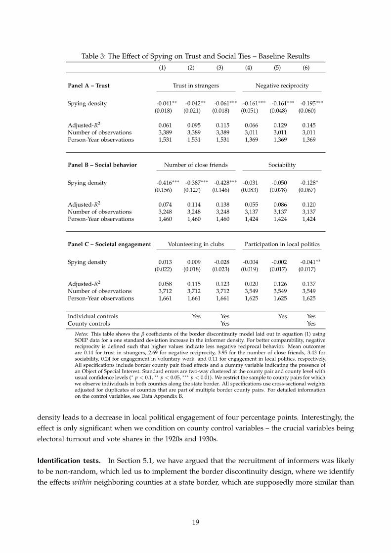
Table 3: The Effect of Spying on Trust and Social Ties – Baseline Results(1) (2) (3) (4) (5) (6)

Panel A – Trust Trust in strangers Negative reciprocity

Spying density -0.041∗∗ -0.042∗∗ -0.061∗∗∗ -0.161∗∗∗ -0.161∗∗∗ -0.195∗∗∗

(0.018) (0.021) (0.018) (0.051) (0.048) (0.060)

Adjusted-R2 0.061 0.095 0.115 0.066 0.129 0.145Number of observations 3,389 3,389 3,389 3,011 3,011 3,011Person-Year observations 1,531 1,531 1,531 1,369 1,369 1,369

Panel B – Social behavior Number of close friends Sociability

Spying density -0.416∗∗∗ -0.387∗∗∗ -0.428∗∗∗ -0.031 -0.050 -0.128∗

(0.156) (0.127) (0.146) (0.083) (0.078) (0.067)


Panel C – Societal engagement Volunteering in clubs Participation in local politics

Spying density 0.013 0.009 -0.028 -0.004 -0.002 -0.041∗∗

(0.022) (0.018) (0.023) (0.019) (0.017) (0.017)


Individual controls Yes Yes Yes YesCounty controls Yes Yes

Notes: This table shows the β coefficients of the border discontinuity model laid out in equation (1) usingSOEP data for a one standard deviation increase in the informer density. For better comparability, negativereciprocity is defined such that higher values indicate less negative reciprocal behavior. Mean outcomesare 0.14 for trust in strangers, 2.69 for negative reciprocity, 3.95 for the number of close friends, 3.43 forsociability, 0.24 for engagement in voluntary work, and 0.11 for engagement in local politics, respectively.All specifications include border county pair fixed effects and a dummy variable indicating the presence ofan Object of Special Interest. Standard errors are two-way clustered at the county pair and county level withusual confidence levels (∗ p < 0.1, ∗∗ p < 0.05, ∗∗∗ p < 0.01). We restrict the sample to county pairs for whichwe observe individuals in both counties along the state border. All specifications use cross-sectional weightsadjusted for duplicates of counties that are part of multiple border county pairs. For detailed informationon the control variables, see Data Appendix B.

density leads to a decrease in local political engagement of four percentage points. Interestingly, theeffect is only significant when we condition on county control variables – the crucial variables beingelectoral turnout and vote shares in the 1920s and 1930s.

Identification tests. In Section 5.1, we have argued that the recruitment of informers was likelyto be non-random, which led us to implement the border discontinuity design, where we identifythe effects within neighboring counties at a state border, which are supposedly more similar than

19

randomly drawn counties. In the following, we provide two identification tests to underscore theimportance of our identification strategy.

A first and simple test is to estimate equation (1) using a naive OLS estimator, i.e., withoutrestricting the sample to counties at borders and ignoring border county pair fixed effects νb. Column(1) of Table 4 provides the results for a such a model. The estimate in column (1) of Panel A shows,for instance, a positive correlation between the spying density and trust in strangers. When restrictingthe sample to counties at state borders but ignoring the fixed effects νb (column (2)), the sign flipsand we see a small but insignificant negative effect. Column (3) restates our preferred specificationfrom Table 3 including county pair fixed effects. A similar pattern can be observed for the othermeasures of trust and social behavior: coefficients become more negative and more significant whenmoving from specification (1) to our preferred model reported in column (3).

In a second test, we try to rule out that our results are driven by long-lasting and persistent culturaldifferences across regions (see, e.g., Becker et al., 2016, for the Habsburg Empire). Specifically, weexploit a territorial reform that happened shortly after the foundation of the GDR. Prior to World WarII, the territory of the GDR was covered by the Free States (and prior monarchies) of Prussia, Saxony,Anhalt, Mecklenburg and Thuringa. When implementing socialism, the GDR regime explicitly triedto overcome this federal structure. It limited the power of sub-national jurisdictions and establisheda centralist state following the example of the Soviet Union. In 1947, the Soviet occupying powerdissolved the state of Prussia and formed the new administrative jurisdictions Mecklenburg, Anhalt,Brandenburg, Thuringa and Saxony. In 1952, fourteen new states (Bezirke) were created; East Berlinbecame the 15th state in 1961. The borderlines were drawn with regard to economic and militaryconsiderations, while cultural and ethnic factors played a minor role. As a result, the new stateborders often separated regions, which had belonged to the same province and shared the samecultural heritage for a long time. We test whether effects of the spying density are different in countypairs that historically belonged to the same Prussian province or Free State. Column (4) of Table4 shows the results. Reassuringly, we find either similar or stronger effects for county pairs thatbelonged to the same region. Thus, it seems unlikely that deep cultural differences at historical stateborders drive the results of our analysis. In particular, we find a significantly negative effect forvolunteering in clubs, which was insignificant in the baseline specification.

20

Table 4: The Effect of Spying on Trust and Social Ties – Identification TestsFull Sample County Pair Sample

(1) (2) (3) (4)

A – Trust in strangersSpying density 0.019 -0.005 -0.061∗∗∗

(0.015) (0.021) (0.018)Spying density × Different Weimar Province -0.071∗∗∗

(0.027)Spying density × Same Weimar Province -0.052∗∗∗

(0.020)Person-Year observations 3,313 1,531 1,531 1,531

B – Negative reciprocitySpying density -0.105∗∗ -0.166∗∗∗ -0.195∗∗∗

(0.046) (0.054) (0.060)Spying density × Different Weimar Province -0.147



C – Number of close friendsSpying density -0.237∗∗ -0.118 -0.428∗∗∗

(0.117) (0.154) (0.146)Spying density × Different Weimar Province -0.483∗∗

(0.198)Spying density × Same Weimar Province -0.379∗∗


D – SociabilitySpying density -0.028 -0.090 -0.128∗

(0.046) (0.058) (0.067)Spying density × Different Weimar Province 0.021



E – Volunteering in clubsSpying density 0.025∗ -0.014 -0.028

(0.014) (0.021) (0.023)Spying density × Different Weimar Province 0.000

(0.028)Spying density × Same Weimar Province -0.054∗∗


F – Participation in local politicsSpying density 0.001 -0.013 -0.041∗∗

(0.010) (0.013) (0.017)Spying density × Different Weimar Province -0.017



County Pair Fixed Effects Yes Yes

Notes: This table shows the β coefficients using different specifications on the base and on the border countypair sample for a one standard deviation increase in the informer density. Mean outcomes are 0.14 for trustin strangers, 2.69 for negative reciprocity, 3.95 for the number of close friends, 3.43 for sociability, 0.24 forengagement in voluntary work, and 0.11 for engagement in local politics, respectively. All regressions includethe full set of controls (see Data Appendix B). Standard errors are two-way clustered at the county and theindividual level in the full sample, and two-way clustered at the county pair and county level in the countypair sample. The usual confidence levels apply (∗ p < 0.1, ∗∗ p < 0.05, ∗∗∗ p < 0.01). We restrict the sample tocounty pairs for which we observe individuals in both counties along the state border. In column (1), cross-sectional weights are used. In columns (2)-(4), cross-sectional weights are adjusted for duplicates of countiesthat are part of multiple border county pairs. 21

6.2 Effects on economic performance

In the previous section, we demonstrated that a higher informer density undermined trust and ledindividuals to scale back their social activities. As social interactions are reduced and exchangingof ideas is less likely, we expect to observe negative economic consequences in counties with moregovernment surveillance. We test this hypothesis in the following section.

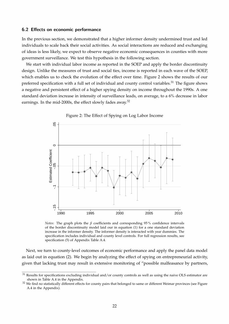
We start with individual labor income as reported in the SOEP and apply the border discontinuitydesign. Unlike the measures of trust and social ties, income is reported in each wave of the SOEP,which enables us to check the evolution of the effect over time. Figure 2 shows the results of ourpreferred specification with a full set of individual and county control variables.31 The figure showsa negative and persistent effect of a higher spying density on income throughout the 1990s. A onestandard deviation increase in intensity of surveillance leads, on average, to a 6% decrease in laborearnings. In the mid-2000s, the effect slowly fades away.32

Figure 2: The Effect of Spying on Log Labor Income

-.15

-.1

-.05

0.0

5E

stim

ated

Coe

ffici

ent

1990 1995 2000 2005 2010

Notes: The graph plots the β coefficients and corresponding 95 % confidence intervalsof the border discontinuity model laid our in equation (1) for a one standard deviationincrease in the informer density. The informer density is interacted with year dummies. Thespecification includes individual and county level controls. For full regression results, seespecification (5) of Appendix Table A.4.

Next, we turn to county-level outcomes of economic performance and apply the panel data modelas laid out in equation (2). We begin by analyzing the effect of spying on entrepreneurial activity,given that lacking trust may result in extensive monitoring of “possible malfeasance by partners,

31 Results for specifications excluding individual and/or county controls as well as using the naive OLS estimator areshown in Table A.4 in the Appendix.

32 We find no statistically different effects for county pairs that belonged to same or different Weimar provinces (see FigureA.4 in the Appendix).

22

employees, and suppliers [and] less time to devote to innovation in new products or processes”(Knack and Keefer, 1997). Indeed, many studies have shown that more trustful people are morelikely to become entrepreneurs (Welter, 2012, Caliendo et al., 2014). We find a negative and quitepersistent effect of the spying density on self-employment rate (see Figure 3).33 The estimate impliesthat for a one standard deviation increase in the spying density, the self-employment rate would bearound 0.4 percentage points lower. Figure 3 also contains information on the potential endogeneityof the intensity of surveillance. If estimates of the intensity of spying were significant prior to WorldWar II, the allocation of spies would have responded to pre-treatment trends in self-employmentrates and would thus have been endogenous in this respect. Reassuringly, we find a remarkably flatpre-trend. Moreover, full regression results show that the estimate is robust as soon as we control forstate times year fixed effects (see Table A.6).

Figure 3: The Effect of Spying on Self-Employment Rates

-1-.

50

.5E

stim

ated

Coe

ffici

ent

1925 1933 1989 1994 1999 2004 2009

Notes: This graph plots the βt coefficients and 95 % confidence intervals of the panel datamodel laid out in equation (2) for a one standard deviation increase in the informer density.The unweighted average post-reunification self-employment rate across counties is 10.42 %.The specification includes county fixed effects and state times year fixed effects as well ascontrols for Objects of Special Interest, county size, opposition and industry composition.See specification (5) in Table A.6 for details.

With entrepreneurial spirit lagging behind, we also expect negative effects on more comprehensivemeasures of economic performance. Ideally, we would look at the effect of spying density on GDP.Unfortunately, there is no pre World War II county-level measure available that is comparable totoday’s GDP. Hence, we take two other proxies for economic performance for which pre-treatmentinformation is available: unemployment rates, and population size (Redding and Sturm, 2008).Figure 4 shows that unemployment is indeed higher in counties with a higher informer density. The33 As explained in Section 3.3, there is no information on self-employment and unemployment rates at the county level in

the early 1990s.

23

Figure 4: The Effect of Spying on Unemployment Rates

0.5

11.

5E

stim

ated

Coe

ffici

ent

1933 1989 1994 1999 2004 2009

Notes: This graph plots the βt coefficients and 95 % confidence intervals of the panel datamodel laid out in equation (2) for a one standard deviation increase in the informer density.The unweighted average post-reunification unemployment rate across counties is 18.66 %.The specification includes county fixed effects and state times year fixed effects as well ascontrols for Objects of Special Interest, county size, opposition and industry composition.See specification (5) in Table A.7 for details.

effect is persistent and oscillates around an increase of 0.6 percentage points in county unemploymentfor a one standard deviation increase in the informer density. Unfortunately, there is only one reliablepre-treatment observation for the unemployment rate. While we can still identify the effect of spyingin our panel research design, we cannot check for pre-trends in unemployment.

Next, we investigate the effect of state surveillance on county population. We start in Panel A ofFigure 5 by plotting the overall average yearly and cumulated county-level population growth ratesfor East Germany since the mid 1980s. The graph shows two emigration waves after the fall of theIron Curtain – a severe and rather short one immediately after reunification (between 1989 and 1992),and a moderate and longer one starting in 1998 (cf. also Fuchs-Schundeln and Schundeln, 2009).In Panel B of Figure 5, we show that the effect of Stasi spying coincides with these two emigrationwaves.34 First, the population in higher-spying counties sharply drops in the first post-treatmentyear 1989.35 This implies that the initial emigration wave was significantly driven by people leavinghigher-spying counties. For 1989, the estimates imply that a one standard deviation decrease inthe spying density yields an increase in the population level of 1.2 percent. Given that the average

34 Effects are always relative to lower spying counties. Hence, a negative population effect does not need to result in alower number of inhabitants if population levels increased in lower spying counties. Given that populations dropped inalmost all counties, the most relevant interpretation of a negative effect seems to be a faster decline in population.

35 Population is measured on December 31, 1989, hence hardly two months after the fall of the Berlin Wall. However,many people already tried to escape from the GDR in the summer of 1989, either via Hungary and Austria or by fleeingto the West German embassies in Warsaw, Prague, and Budapest.

24

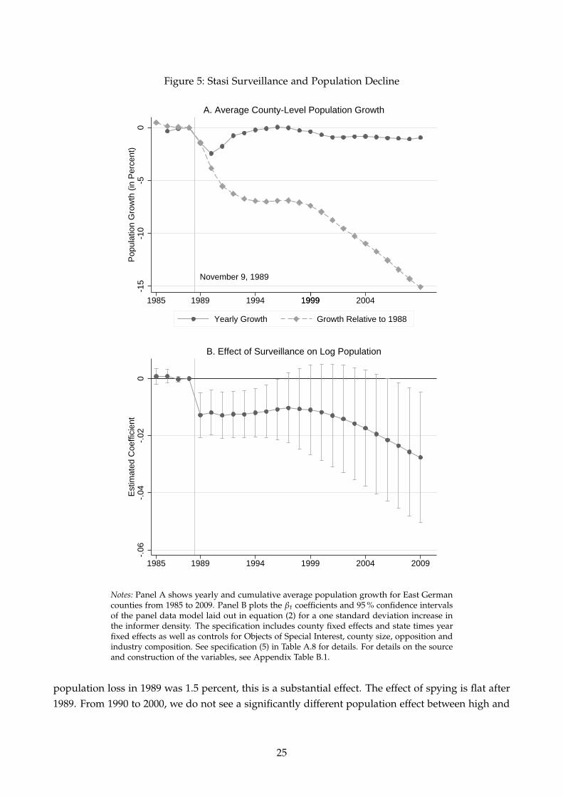
Figure 5: Stasi Surveillance and Population Decline

November 9, 1989

-15

-10

-50

Pop

ulat

ion

Gro

wth

(in

Per

cent

)

1985 1989 1994 1999 20041999

Yearly Growth Growth Relative to 1988

A. Average County-Level Population Growth

-.06

-.04

-.02

0E

stim

ated

Coe

ffici

ent

1985 1989 1994 1999 2004 2009

B. Effect of Surveillance on Log Population

Notes: Panel A shows yearly and cumulative average population growth for East Germancounties from 1985 to 2009. Panel B plots the βt coefficients and 95 % confidence intervalsof the panel data model laid out in equation (2) for a one standard deviation increase inthe informer density. The specification includes county fixed effects and state times yearfixed effects as well as controls for Objects of Special Interest, county size, opposition andindustry composition. See specification (5) in Table A.8 for details. For details on the sourceand construction of the variables, see Appendix Table B.1.

population loss in 1989 was 1.5 percent, this is a substantial effect. The effect of spying is flat after1989. From 1990 to 2000, we do not see a significantly different population effect between high and

25

low-spying counties in addition to the initial population outflow. This implies that the populationresponse driven by spying was immediate. In 2001, i.e., in the early years of the second emigrationwave, the effect of spying on population size starts to decline again and continues to do so until 2009.

6.3 Discussion: Alternative channels and indirect effects

In the previous two sections, we demonstrated various reduced form effects of the spying density ontrust, social ties and economic performance. These estimates quantify the total effect of governmentsurveillance, which is the main focus of this study. In the following section, we take a closer look atpotential mechanisms behind these overall effects. First, we corroborate that government surveillanceis indeed driving our results by ruling out alternative channels such as socialist indoctrination orpost-reunification subsidies. In a second step, we assess the role of indirect second-round effects.Specifically, we analyze whether negative effects on trust and social ties are simply driven by localeconomic or population shocks.

We start by exploring the role of alternative channels that might potentially explain the declinein trust, social ties and economic performance. As socialist indoctrination has been shown toaffect individual preferences and economic outcomes (see, e.g., Alesina and Fuchs-Schundeln, 2007,Fuchs-Schundeln and Masella, 2016), it might also be a potential driver of our effects. While thementioned studies compared East to West Germany, we have to find a measure that can pick upregional variation in the ideological penetration within the East German society. Given that the GDRregime was a one-party dictatorship, we proxy socialist indoctrination by the share of SED partymembers among the political and economic elites in 1988 (see Appendix Table B.1 for details onthis variable). In a first step, we show that our measure of socialist indoctrination is only weaklycorrelated with the intensity of surveillance. Moreover, as soon as we condition on control variables,there is virtually no correlation between the two variables (see Figure A.5 in the Appendix). Second,we demonstrate that estimates are basically unchanged when including the indoctrination variableas a control (see column (2) of Tables 5 and A.5; column (6) of Tables A.6 to A.8).36

An alternative driver of our results might be government transfers and subsidies that were paid toEast German counties after reunification in order to rebuild public infrastructure and the housingstock (Aufbau Ost). These subsidies, which, for instance, caused a boom in the construction sector(Paque, 2009), might thus be correlated with the informer density via the industrial structure of acounty. Although we control for the industrial structure in our baseline specification, we additionallyinclude the annual sum of government subsidies paid to the specific counties. Results are not affectedby these controls either (see column (3) of Tables 5 and A.5; column (7) of Tables A.6 to A.8).37

While these tests suggest that government surveillance is the driver of our results, we take acloser look at the implied mechanism, that is, surveillance affecting trust and social ties, whichtriggers negative economic effects. For this reason, we assess the importance of indirect effects in theremainder of this section. First, we consider the role of economic shocks, which might also lead to

36 Column (1) of Tables 5 and A.5 replicate the main results of Tables 3 and A.4 on a sample that excludes East Berlinand the respective border county pairs. We exclude East Berlin throughout Tables 5 and A.5 because we do not haveseparate population data for East and West Berlin after reunification, which is necessary to control for changes in thepopulation (see below). Note that no result is driven by the restriction of the sample.

37 We have no information on transfers for the years 1990–1994.

26

lower levels of trust and social withdrawal. In order to rule out this mechanism, we first reestimateour preferred specification of equation (1), including county-level income as an additional controlvariable.38 Comparing the baseline specification and the model conditional on county-level income(see columns (1) and (4) of Table 5), we find that results are almost identical.39

It is equally possible that negative effects on trust and social ties are driven by the substantialoverall migration response. In order to capture the consequences of these population shocks, weinclude the county-level population growth rate as an additional control variable. Results provided incolumn (5) of Table 5 change only slightly.40 We also find that effects on individual labor income arerobust when additionally controlling for population growth, see Table A.5, column (4). As regardsour county-level results, all economic outcomes are measured as rates, hence the estimates alreadyaccount for base changes due to migration. However, we additionally check the robustness of ourestimates by including log current population in order to check whether our findings are driven byagglomeration effects. Estimates, presented in columns (8) of Tables A.6 through A.7, are hardlyaffected.

While overall migration does not exhibit substantial second-round effects, it is still possible thatresults are triggered by selective out-migration. In the border discontinuity design, our preferredspecification accounts for selective out-migration by conditioning on a large set of individual controls.Introducing these controls, which capture compositional differences within county pairs, hardlyaffects our results (cf. Tables 3 and A.4). This indicates that selective out-migration is not a keydriver of the results, either. In addition, we provide a second, more immediate test for selectiveout-migration using the panel data design. Here, we directly test whether the spying density had aneffect on specific population shares. In terms of skills, Figure 6 shows that, if anything, there is asmall positive effect of the Stasi on the share of high-skilled employees in a county. A one standarddeviation increase in the intensity of surveillance leads to an (insignificant) increase of 0.2 percentagepoints in the share of the high-skilled. This finding is in line with Fuchs-Schundeln and Schundeln(2009), who show that the first migration wave (1989–1992) was rather driven by individuals withouta college degree or vocational training. In Figure 7, we further assess the evolution of populationshares by age groups. The initial population shock of the first wave (1989–1992) seems to be drivenby individuals who were 35-54 years old and had no children at that time. In contrast, with the onsetof the second immigration wave starting in the late 1990s, the share of 15-34 year olds graduallystarts to decline in higher-spying counties. Overall, the results on population shares do not providestrong evidence for selective out-migration. While the effect on the share of high-skilled individualspoints to a negative selection out of high-spying counties, which, ceteris paribus, should be beneficialfor economic outcomes, the effects by age are inconclusive but hint at a decreasing share of youngindividuals starting in the late 1990s. In general, the magnitudes of these effects are very small,which suggests a marginal role of indirect migration effects.

38 We are aware that income itself is an outcome and that we are sacrificing econometric rigor with such a specification.Yet, we think that learning more about the underlying mechanisms is interesting and important, and thus justifiessuch a specification as a robustness test. In any case, we interpret the following results carefully and regard them assuggestive rather than definitive.

39 Results do not change when including individual labor income rather than the mean county-level income.40 As mentioned above, we assign each individual the informer density of the GDR county in which she lived in 1989,

which prevents selection out-of-treatment in the first place.

27

Table 5: The Effect of Spying on Trust and Social Ties – Exploring the mechanismCounty Pair Sample

(1) (2) (3) (4) (5) (6)

A – Trust in strangersSpying density -0.066∗∗∗ -0.046∗∗∗ -0.079∗∗∗ -0.066∗∗∗ -0.056∗∗∗ -0.056∗∗∗

(0.019) (0.014) (0.021) (0.018) (0.021) (0.018)Person-Year observations 1,285 1,285 1,285 1,285 1,285 1,285

B – Negative reciprocitySpying density -0.166∗∗∗ -0.192∗∗∗ -0.184∗∗∗ -0.166∗∗∗ -0.191∗∗∗ -0.194∗∗∗


C – Number of close friendsSpying density -0.426∗∗∗ -0.397∗∗∗ -0.495∗∗∗ -0.429∗∗∗ -0.314∗ -0.430∗∗∗


D – SociabilitySpying density -0.188∗∗∗ -0.181∗∗∗ -0.144∗∗ -0.190∗∗∗ -0.141∗∗ -0.115∗


E – Volunteering in clubsSpying density -0.029 -0.034 -0.034 -0.030 -0.036 -0.046∗


F – Participation in local politicsSpying density -0.041∗∗ -0.042∗∗ -0.036∗ -0.043∗∗ -0.044∗∗ -0.042∗∗


Individual controls Yes Yes Yes Yes Yes YesCounty controls Yes Yes Yes Yes Yes YesShare SED party members Yes YesGovernment transfers Yes YesMean county-level income Yes YesPopulation growth Yes Yes

Notes: This table shows the β coefficients of the border discontinuity model laid out in equation (1)using SOEP data for a one standard deviation increase in the informer density. For better comparabil-ity, negative reciprocity is defined such that higher values indicate less negative reciprocal behavior.Mean outcomes are 0.14 for trust in strangers, 2.69 for negative reciprocity, 3.95 for the number ofclose friends, 3.43 for sociability, 0.24 for engagement in voluntary work, and 0.11 for engagement inlocal politics, respectively. All specifications include county pair fixed effects and a dummy variableindicating the presence of an Object of Special Interest. Standard errors are two-way clustered at thecounty pair and county level with usual confidence levels (∗ p < 0.1, ∗∗ p < 0.05, ∗∗∗ p < 0.01). Werestrict the sample to county pairs for which we observe individuals in both counties along the stateborder. All specifications use cross-sectional weights adjusted for duplicates of counties that are partof multiple county pairs. For detailed information on the control variables, see Data Appendix B.

28

Figure 6: The Effect of Spying on Share of High-Skilled

-.2

0.2

.4.6

Est

imat

ed C

oeffi

cien

t

1989 1994 1999 2004 2009

Notes: This graph plots the βt coefficients and 95 % confidence intervals of the panel datamodel laid out in equation (2) for a one standard deviation increase in the informer density.The unweighted average post-reunification high-skill share across counties is 3.98 %. Thespecification includes county fixed effects and state times year fixed effects as well ascontrols for Objects of Special Interest, county size, opposition and industry composition.See specification (5) in Table A.9 for details.

29

Figure 7: Stasi Surveillance and Age Groups

-.3

-.2

-.1

0.1

.2E

stim

ated

Coe

ffici

ent

1989 1994 1999 2004 2009

A. Population Share below 15

-1-.

50

.5E

stim

ated

Coe

ffici

ent

1989 1994 1999 2004 2009

B. Population Share 15--34

-.5

0.5

1E

stim

ated

Coe

ffici

ent

1989 1994 1999 2004 2009

C. Population Share 35--54

-.2

0.2

.4.6

.8E

stim

ated

Coe

ffici

ent

1989 1994 1999 2004 2009

D. Population Share above 54

Notes: This graph plots the βt coefficients and 95 % confidence intervals of the panel datamodel laid out in equation (2) for a one standard deviation increase in the informer density.Panel A shows the effect of spying on the share of the population younger than 15, Panel Bthe effect on the group between 15–34, Panel C the effect on the group 35–54 and Panel Dthe effect on the group older than 54. The unweighted average post-reunification populationshares across counties are 14.08 %, 25.35 %, 29.87 %, 30.70 %, respectively. The specificationincludes county fixed effects and state times year fixed effects as well as controls for Objectsof Special Interest, county size, opposition and industry composition. See specification (5)in Tables A.10–A.13 for details.

30

7 Conclusion

In this paper, we estimate the effect of state surveillance on trust, social ties and economic performanceby exploiting county-level variation in the number of Stasi informers per capita in the former socialistGerman Democratic Republic. To account for the potentially non-random recruitment of informersacross counties, we implement two different research designs. First, we exploit discontinuities atstate borders arising from the administrative structure of the Ministry for State Security. Second,we set up a long-term panel including pre World War II measures of economic performance, whichallows us to control for county fixed effects.

Overall, the results of our study offer substantial evidence for negative and long-lasting effects ofgovernment surveillance. We find strong and consistent evidence that a higher density of informersundermined trust and led to a withdrawal from society. In particular, more intense surveillancecaused lower trust in strangers, stronger negative reciprocity, fewer close friends, lower sociability,and reduced societal engagement in clubs and local politics. Against the backdrop of this socialwithdrawal, we also find negative and persistent effects of government surveillance on variousmeasures of economic performance, such as individual labor income, county-level self-employment,unemployment and population size. We provide evidence that these results are indeed caused bygovernment surveillance and not driven by alternative factors such as socialist indoctrination.

Our findings have important implications for contemporary forms of government surveillancein authoritarian, but also in democratic countries. Given that all surveillance programs extractinformation from social networks, it is likely that the current systems in authoritarian states likeChina or Russia exert similar negative effects on social interactions and economic performance.Moreover, the social and economic costs of surveillance should also be taken into account bybenevolent governments when designing the optimal surveillance policy.

Our results also add to the large literature on institutions. Following the terminology of Alesinaand Giuliano (2015), our study establishes a causal link running from formal institutions to culture,as measured by trust and social behavior. We show that this effect is still visible many years after thefall of the Berlin Wall and the end of the socialist East German regime. Moreover, and in line withTabellini (2010), we provide clear evidence that the degree of democratic governance affects economicoutcomes. With both trust and economic performance being impaired by government surveillance,our findings also provide suggestive evidence in favor of a well established channel: institutionsshape peoples’ trust, and trust affects economic development (Algan and Cahuc, 2014). In particular,and in line with La Porta et al. (1997), our findings point to reduced entrepreneurial activity as animportant channel for the observed economic decline. As for our measures of trust and social ties,these effects are persistent and detectable two decades after the end of the socialist regime. Given theintergenerational transmission of trust and beliefs (see, e.g., Nunn and Wantchekon, 2011, Dohmenet al., 2012), it seems likely that these effects will be even longer-lasting. In fact, the erosion ofcivic capital induced by the Stasi surveillance system could be one explanatory factor of the lackingconvergence between East and West Germany.

31

References

Acemoglu, D., Naidu, S., Restrepo, P. and Robinson, J. A. (2015). Democracy Does Cause Growth.Working paper.

Agrawal, D. R. (2015). The Tax Gradient: Spatial Aspects of Fiscal Competition, American EconomicJournal: Economic Policy 7(2): 1–29.

Albats, Y. (1995). KGB: State Within a State, I.B.Tauris & Co Ltd, London.

Alesina, A. and Fuchs-Schundeln, N. (2007). Goodbye Lenin (or Not?): The Effect of Communism onPeople’s Preferences, American Economic Review 97(4): 1507–1528.

Alesina, A. and Giuliano, P. (2015). Culture and Institutions, Journal of Economic Literature 53(4): 898–944.

Alesina, A., Giuliano, P. and Nunn, N. (2013). On the Origins of Gender Roles: Women and thePlough, The Quarterly Journal of Economics 128(2): 469–530.

Algan, Y. and Cahuc, P. (2010). Inherited Trust and Growth, American Economic Review 100(5): 2060–2092.

Algan, Y. and Cahuc, P. (2014). Trust, Growth, and Well-Being: New Evidence and Policy Implications,in P. Aghion and S. Durlauf (eds), Handbook of Economic Growth, North Holland, Elsevier.

Anderson, P. (2016). Fighting ’Terrorism’, Repressing Democracy: Surveillance and Resistance in theUK, Warwick School of Law Research Paper No. 2016/1.

Arendt, H. (1951). The Origins of Totalitarianism, Harcourt, Brace and Company, New York.

Arrow, K. J. (1972). Gifts and Exchanges, Philosophy & Public Affairs 1(4): 343–362.

Becker, S., Boeckh, K., Hainz, C. and Woßmann, L. (2016). The Empire Is Dead, Long Live theEmpire! Long-Run Persistence of Trust and Corruption in the Bureaucracy, The Economic Journal126(590): 40–74.

Becker, S. O. and Woßmann, L. (2009). Was Weber Wrong? A Human Capital Theory of ProtestantEconomic History, The Quarterly Journal of Economics 124(2): 531–596.

Branigan, T. (2010). Chinese police chief boasts of recruiting one in 33 residents as informants, TheGuardian, Februrary 10, 2010.URL: https://www.theguardian.com/world/2010/feb/10/china-police-informants-surveillance

Bruce, G. (2010). The Firm – The Inside Story of the Stasi, Oxford University Press, New York.

Burchardi, K. B. and Hassan, T. A. (2013). The Economic Impact of Social Ties: Evidence fromGerman Reunification, The Quarterly Journal of Economics 128(3): 1219–1271.

Butler, J., Giuliano, P. and Guiso, L. (2016). The Right Amount of Trust, Journal of European EconomicAssociation forthcoming.

32

Caliendo, M., Fossen, F. and Kritikos, A. S. (2014). Personality characteristics and the decisions tobecome and stay self-employed, Small Business Economics 42(4): 787–814.

Capon, F. (2015). ’Soviet-era snitching’ returns to Russia, Newsweek, June 1, 2015.URL: http://europe.newsweek.com/soviet-era-snitching-returns-russia-328036

Deng, Y. and O’Brien, K. J. (2013). Relational Repression in China: Using Social Ties to DemobilizeProtesters, The China Quarterly 215: 1–20.

Dohmen, T., Falk, A., Huffman, D. and Sunde, U. (2009). Homo Reciprocans: Survey Evidence OnBehavioural Outcomes, The Economic Journal 119(3): 592–612.

Dohmen, T., Falk, A., Huffman, D. and Sunde, U. (2012). The Intergenerational Transmission of Riskand Trust Attitudes, Review of Economic Studies 79: 645–677.

Dube, A., Lester, T. W. and Reich, M. (2010). Minimum wage effects across state borders: Estimatesusing contiguous counties, Review of Economics and Statistics 92(4): 945–964.

Falter, J. W. and Hanisch, D. (1990). Election and Social Data of the Districts and Municipalities of theGerman Empire from 1920 to 1933, GESIS Data Archive, Cologne (ZA8013). DOI: 10.4232/1.8013.

Fontana, N., Nannicini, T. and Tabellini, G. (2016). Historical Roots of Political Extremism: the Effectsof Nazi Occupation of Italy, Working Paper .

Friehe, T., Pannenberg, M. and Wedow, M. (2015). Let Bygones be Bygones? Socialist Regimes andPersonalities in Germany, SOEPpapers 776.

Fuchs-Schundeln, N. and Hassan, T. A. (2015). Natural Experiments in Macroeconomics, NBERWorking Paper No. 21228.

Fuchs-Schundeln, N. and Masella, P. (2016). Long-Lasting Effects of Socialist Education, Review ofEconomics and Statistics (forthcoming). DOI: 10.1162/REST a 00583.

Fuchs-Schundeln, N. and Schundeln, M. (2009). Who stays, who goes, who returns? East – Westmigration within Germany since reunification, Economics of Transition 17: 703–738.

Gieseke, J. (1995). Diskussion, in K.-D. Henke and R. Engelmann (eds), Aktenlage. Die Bedeutungder Unterlagen des Staatssicherheitsdienstes fur die Zeitgeschichtsforschung, Ch. Links Verlag, Berlin,pp. 189–192.

Gieseke, J. (2014). The History of the Stasi: East Germany’s Secret Police, 1945–1990, Berghahn Books,New York, Oxford.

Glaeser, E. L., Laibson, D. I., Scheinkman, J. A. and Soutter, C. L. (2000). Measuring Trust, TheQuarterly Journal of Economics 115(3): 811–846.

Glitz, A. and Meyersson, E. (2016). Industrial espionage and productivity, Working Paper, March.

33

Goodchild, M. F. and Lam, N. S.-N. (1980). Areal Interpolation: A Variant of the Traditional SpatialProblem, Geo-Processing 1: 297–312.

Grashoff, U. (2011). Schwarzwohnen. Die Unterwanderung der staatlichen Wohnraumlenkung in der DDR,V&R unipress, Gottingen.

Guiso, L., Sapienza, P. and Zingales, L. (2006). Does Culture Affect Economic Outcomes?, Journal ofEconomic Perspectives 20(2): 23–48.

Haggerty, K. and Samatas, M. (2010). Surveillance and Democracy: an unsettled relationship,Routledge, pp. 1–16.

Hall, R. E. and Jones, C. I. (1999). Why do Some Countries Produce So Much More Output PerWorker than Others?, The Quarterly Journal of Economics 114(1): 83–116.

Harrison, M. and Zaksauskiene, I. (2015). Counter-intelligence in a command economy, EconomicHistory Review 69(1): 131–158.

Holmes, T. J. (1998). The Effect of State Policy on the Location of Manufacturing: Evidence fromState Borders, Journal of Political Economy 106(4): 667–705.

Horsch, H. (1997). “Hat nicht wenigstens die Stasi die Stimmung im Lande gekannt?” MfS undSED im Bezirk Karl-Marx-Stadt. Die Entmachtung der Staatssicherheit in den Regionen, Teil 3, BFinformiert 19/1997.

infas (n.d.). DDR-Kreisstrukturdaten, infas-Absatzplanung, Munchen.

Jacob, M. and Tyrell, M. (2010). The Legacy of Surveillance: An Explanation for Social Capital Erosionand the Persistent Economic Disparity between East and West Germany. Mimeo, presented at theSciences Po/IZA Workshop on “Trust, Civic Spirit and Economic Performance” in June 2010.

Jacobs, A. and Ansfield, J. (2011). Well-Oiled Security Apparatus in China Stifles Calls for Change,The New York Times, February 28, 2011.URL: http://www.nytimes.com/2011/03/01/world/asia/01china.html

King, G., Rosen, O., Tanner, M. and Wagner, A. F. (2008). Ordinary Economic Voting Behavior in theExtraordinary Election of Adolf Hitler, The Journal of Economic History 68(4): 951–996.

Knabe, H. (1999). Die feinen Waffen der Diktatur. Nicht-strafrechtliche Formen politischer Verfolgungin der DDR, in H. Timmermann (ed.), Die DDR – Erinnerungen an einen untergegangenen Staat,Vol. 88 of Dokumente und Schriften der Europaischen Akademie Otzenhausen, Duncker & Humboldt,Berlin, pp. 191–220.

Knack, S. and Keefer, P. (1997). Does Social Capital Have an Economic Payoff? A Cross-CountryInvestigation, The Quarterly Journal of Economics 112(4): 1251–1288.

Kowalczuk, I.-S. (2009). Endspiel. Die Revolution von 1989 in der DDR, C.H.Beck, Munchen.

34

La Porta, R., Lopez-De-Silane, F., Shleifer, A. and Vishny, R. W. (1997). Trust in Large Organizations,American Economic Review: Papers and Proceedings 87(2): 333–338.

Lichtbaum, E. and Apuzzo, M. (2016). Orlando Gunman Was on Terror Watchlist, F.B.I. Director Says,New York Times, June 13, 2016, http://www.nytimes.com/2016/06/14/us/omar-mateen-fbi.html.

Magruder, J. R. (2012). High Unemployment Yet Few Small Firms: The Role of Centralized Bargainingin South Africa, American Economic Journal: Applied Economics 4(3): 138–166.

Mauro, P. (1995). Corruption and Growth, The Quarterly Journal of Economics 110(3): 681–712.

Max Planck Institute for Demographic Research (MPIDR) and Chair for Geodesy and Geoinformatics,University of Rostock (CGG) (2011). MPIDR Population History GIS Collection, Rostock. (Partlybased on Hubatsch, W. and T. Klein (eds) 1975 ff.: Grundriß der deutschen Verwaltungsgeschichte,Marburg, and Bundesamt fur Kartographie und Geodasie: VG 2500 Verwaltungsgebiete [Ebenen]1:2.500.000, Stand 01.01.2009, Frankfurt am Main).

Moser, P., Voena, A. and Waldinger, F. (2014). German Jewish Emigres and US Invention, AmericanEconomic Review 104(10): 3222–3255.

Muller-Enbergs, H. (1996). Inoffizielle Mitarbeiter des Ministeriums fur Staatssicherheit. Richtlinien undDurchfuhrungsbestimmungen, Ch. Links Verlag, Berlin.

Muller-Enbergs, H. (2008). Inoffizielle Mitarbeiter des Ministeriums fur Staatssicherheit. Teil 3: Statistik,Ch. Links Verlag, Berlin.

Muller-Enbergs, H. (2013). Warum wird einer IM? Zur Motivation bei der inoffiziellen Zusam-menarbeit mit dem Staatssicherheitsdienst, in K. Behnke and J. Fuchs (eds), Zersetzung der Seele.Psychologie und Psychiatrie im Dienste des MfS, 4 edn, CEP Europaische Verlagsanstalt, Hamburg,pp. 102–129.

Niemann, M. (2007). Die Sekretare der SED-Bezirksleitungen 1952 bis 1989, Ferdinand Schoningh,Paderborn.

Nunn, N. (2008). The Long-Term Effects of Africa’s Slave Trades, The Quarterly Journal of Economics123(1): 139–176.

Nunn, N. and Wantchekon, L. (2011). The Slave Trade and the Origins of Mistrust in Africa, AmericanEconomic Review 101(7): 3221–3252.

Paque, K.-H. (2009). Die Bilanz. Eine wirtschaftliche Analyse der Deutschen Einheit, Hanser.

Pew Research Center (2014). Spring political typology survey, http://www.pewresearch.org/fact-tank/2015/05/29/what-americans-think-about-nsa-surveillance-national-security-and-privacy/.

Putnam, R. (2000). Bowling Alone: The Collapse and Revival of American Community, Simon & Schuster,New York.

35

Putnam, R. D. (1995). Bowling Alone: America’s Declining Social Capital, Journal of Democracy6(1): 65–78.

Redding, S. J. and Sturm, D. (2008). The Costs of Remoteness: Evidence from German Division andReunification, American Economic Review 98(5): 1766–1797.

Reich, J. (1997). Sicherheit und Feigheit – der Kafer im Brennglas, in S. Suckut (ed.), Staatspartei undStaatssicherheit. Zum Verhaltnis von SED und MfS, Ch. Links Verlag, Berlin, pp. 25–37.

Ritter, J. and Lapp, P. J. (1997). Die Grenze. Ein deutsches Bauwerk, Ch. Links Verlag, Berlin.

Rodrik, D., Subramanian, A. and Trebbi, F. (2004). Institutions Rule: The Primacy of Institutions OverGeography and Integration in Economic Development, Journal of Economic Growth 9(2): 131–165.

Rudolph, H. (1990). Beschaftigungsstrukturen in der DDR vor der Wende, Mitteilungen aus derArbeitsmarkt- und Berufsforschung 4: 474–503.

Ruhle, J. and Holzweißig, G. (1988). Der 13. August 1961. Die Mauer von Berlin, 3 edn, EditionDeutschland Archiv, Koln.

Satyanath, S., Voigtander, N. and Voth, H.-J. (2016). Bowling for Fascism: Social Capital and the Riseof the Nazi Party, Journal of Political Economy forthcoming.

Schneier, B. (2013). NSA secrets kill our trust.URL: http://edition.cnn.com/2013/07/31/opinion/schneier-nsa-trust/

Shleifer, A. (1997). Government in Transition, European Economic Review 41: 385–410.

Stabile, E. (2014). Recruiting Terrorism Informants: The Problems with Immigration Incentives andthe S-6 Visa, California Law Review 102(1): 235–276.

Tabellini, G. (2010). Culture and Institutions: Economic Development in the Regions of Europe,Journal of the European Economic Association 8(4): 677–716.

The Economist Intelligence Unit (2014). Democracy index, www.eui.com.

Voigtlander, N. and Voth, H.-J. (2012). Persecution Perpetuated: The Medieval Origins of Anti-SemiticViolence in Nazi Germany, The Quarterly Journal of Economics 127(3): 1339–1392.

Wagner, G. G., Frick, J. R. and Schupp, J. (2007). The German Socio-Economic Panel Study (SOEP):Scope, Evolution and Enhancements, Schmollers Jahrbuch: Journal of Applied Social Science Studies127(1): 139–170.

Welter, F. (2012). All you need is trust? A critical review of the trust and entrepreneurship literature,International Small Business Journal 30(3): 193–212.

Wolf, N. (2009). Was Germany Ever United? Evidence from Intra- and International Trade, 1885–1933,The Journal of Economic History 69(3): 846–881.

36

Wolle, S. (2009). Die heile Welt der Diktatur. Herrschaft und Alltag in der DDR 1971–1989, Ch. LinksVerlag, Berlin.

Yu, M. (2014). Paranoia in Beijing with million-man mobilization of government informants, TheWashington Times, October 23, 2014.URL: http://www.washingtontimes.com/news/2014/oct/23/inside-china-beijing-mobilizes-1-million-informant/

Zak, P. J. and Knack, S. (2001). Trust and Growth, The Economic Journal 111(470): 295–321.

Zurcher, A. (2013). Roman Empire to the NSA: A world history of government spying, BBC NewsMagazine, November 1, 2013.URL: http://www.bbc.com/news/magazine-24749166

37

A Appendix

Figure A.1: Number of Requests for the Inspection of Stasi Files10

020

030

040

050

0N

umbe

r of

req

uest

s (in

1,0

00)

1990 1995 2000 2005 2010

Notes: This graph plots the annual number of requests for inspection of Stasi files. It is basedon data from the Agency of the Federal Commissioner for the Stasi Records.

38

Figure A.2: Alternative Measures of Stasi Surveillance

56

78

Log

tota

l num

ber

of in

form

ers

4 5 6 7 8Log number of operative informers

A. Informer definitions (r=0.95)

23

45

6Lo

g nu

mbe

r of

em

ploy

ees

4 5 6 7 8Log number of operative informers

B. Informers and employees (r=0.81)

Notes: The graph plots the correlation between three different measures of Stasi surveillance:(i) the number of operative informers (unofficial collaborator category 1), which builds thebase for our preferred measure of the informer density, (ii) the total number of informersin categories (1)-(3), and (iii) the number of official Stasi employees in 1982. Correlationcoefficients ρ are presented in parentheses. For information on all variables, see AppendixTable B.1.

39

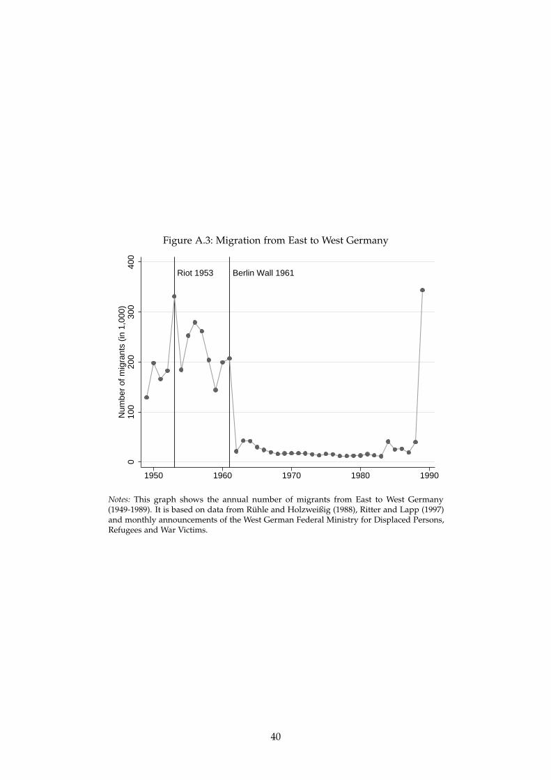
Figure A.3: Migration from East to West Germany

Riot 1953 Berlin Wall 1961

010

020

030

040

0N

umbe

r of

mig

rant

s (in

1,0

00)

1950 1960 1970 1980 1990

Notes: This graph shows the annual number of migrants from East to West Germany(1949-1989). It is based on data from Ruhle and Holzweißig (1988), Ritter and Lapp (1997)and monthly announcements of the West German Federal Ministry for Displaced Persons,Refugees and War Victims.

40

Figure A.4: The Effect of Spying on Log Labor Income

-.15

-.1

-.05

0.0

5.1

Est

imat

ed C

oeffi

cien

t

1990 1995 2000 2005 2010

Different Weimar Province Same Weimar Province

Notes: The graph plots the β coefficients and corresponding 95 % confidence intervals of theborder discontinuity model laid our in equation (1) for a one standard deviation increase inthe informer density. The informer density is interacted with year dummies and a dummyvariable indicating whether a border county pair was part of the same Weimar province.The specification includes individual and county level controls.

41

Figure A.5: Informer Density and Socialist Indoctrination

3040

5060

70S

hare

of e

lites

with

SE

D m

embe

rshi

p

.2 .4 .6 .8 1Share of operative unofficial informers

A. Without control variables (r=0.13)

-15

-10

-50

510

Res

idua

l elit

e sh

are

with

SE

D m

embe

rshi

p

-.2 0 .2 .4 .6Residual share of unofficial informers

B. With control variables (r=-0.01)

Notes: The graph plots the correlation between the share of operative informers in thepopulation and the share of SED party members among political and economic executives.Panel A shows the raw correlation between both measures. Panel B depicts the correlationbetween the residiuals of both variables after regressing them on the full set of controlvariables (see Section 4). For information on all variables, see Appendix Table B.1.

42

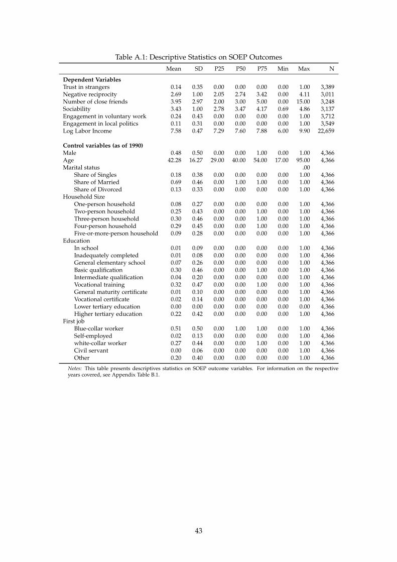
Table A.1: Descriptive Statistics on SOEP OutcomesMean SD P25 P50 P75 Min Max N

Dependent VariablesTrust in strangers 0.14 0.35 0.00 0.00 0.00 0.00 1.00 3,389Negative reciprocity 2.69 1.00 2.05 2.74 3.42 0.00 4.11 3,011Number of close friends 3.95 2.97 2.00 3.00 5.00 0.00 15.00 3,248Sociability 3.43 1.00 2.78 3.47 4.17 0.69 4.86 3,137Engagement in voluntary work 0.24 0.43 0.00 0.00 0.00 0.00 1.00 3,712Engagement in local politics 0.11 0.31 0.00 0.00 0.00 0.00 1.00 3,549Log Labor Income 7.58 0.47 7.29 7.60 7.88 6.00 9.90 22,659

Control variables (as of 1990)Male 0.48 0.50 0.00 0.00 1.00 0.00 1.00 4,366Age 42.28 16.27 29.00 40.00 54.00 17.00 95.00 4,366Marital status .00

Share of Singles 0.18 0.38 0.00 0.00 0.00 0.00 1.00 4,366Share of Married 0.69 0.46 0.00 1.00 1.00 0.00 1.00 4,366Share of Divorced 0.13 0.33 0.00 0.00 0.00 0.00 1.00 4,366

Household SizeOne-person household 0.08 0.27 0.00 0.00 0.00 0.00 1.00 4,366Two-person household 0.25 0.43 0.00 0.00 1.00 0.00 1.00 4,366Three-person household 0.30 0.46 0.00 0.00 1.00 0.00 1.00 4,366Four-person household 0.29 0.45 0.00 0.00 1.00 0.00 1.00 4,366Five-or-more-person household 0.09 0.28 0.00 0.00 0.00 0.00 1.00 4,366

EducationIn school 0.01 0.09 0.00 0.00 0.00 0.00 1.00 4,366Inadequately completed 0.01 0.08 0.00 0.00 0.00 0.00 1.00 4,366General elementary school 0.07 0.26 0.00 0.00 0.00 0.00 1.00 4,366Basic qualification 0.30 0.46 0.00 0.00 1.00 0.00 1.00 4,366Intermediate qualification 0.04 0.20 0.00 0.00 0.00 0.00 1.00 4,366Vocational training 0.32 0.47 0.00 0.00 1.00 0.00 1.00 4,366General maturity certificate 0.01 0.10 0.00 0.00 0.00 0.00 1.00 4,366Vocational certificate 0.02 0.14 0.00 0.00 0.00 0.00 1.00 4,366Lower tertiary education 0.00 0.00 0.00 0.00 0.00 0.00 0.00 4,366Higher tertiary education 0.22 0.42 0.00 0.00 0.00 0.00 1.00 4,366

First jobBlue-collar worker 0.51 0.50 0.00 1.00 1.00 0.00 1.00 4,366Self-employed 0.02 0.13 0.00 0.00 0.00 0.00 1.00 4,366white-collar worker 0.27 0.44 0.00 0.00 1.00 0.00 1.00 4,366Civil servant 0.00 0.06 0.00 0.00 0.00 0.00 1.00 4,366Other 0.20 0.40 0.00 0.00 0.00 0.00 1.00 4,366

Notes: This table presents descriptives statistics on SOEP outcome variables. For information on the respectiveyears covered, see Appendix Table B.1.

43

Table A.2: Descriptive Statistics on Panel Outcomes and ControlsMean SD P25 P50 P75 Min Max N

Self-employment rate1925–1933 18.56 4.17 15.29 18.09 20.92 10.88 31.79 3701996–2009 10.42 2.01 9.00 10.30 11.90 5.00 15.40 2,590

Unemployement rate1933–1933 15.83 5.60 10.89 16.48 20.14 3.70 28.71 1851996–2009 18.66 3.79 16.15 18.61 21.10 6.60 31.28 2,590

Log population1985–1988 11.01 0.56 10.58 10.98 11.32 9.79 13.23 7401989–2009 10.91 0.55 10.53 10.88 11.22 9.63 13.18 3,885

Population share younger than 151989–1989 19.72 1.79 18.60 19.76 20.94 15.56 24.74 1851990–2009 14.08 3.42 11.00 13.42 16.73 8.63 24.62 3,700

Population share aged 15–341989–1989 29.43 1.62 28.25 29.61 30.42 25.52 34.14 1851990–2009 25.35 2.56 23.67 25.59 27.22 18.72 32.93 3,700

Population share aged 35–541989–1989 26.21 1.38 25.31 26.19 26.96 23.06 30.32 1851990–2009 29.87 2.56 27.75 29.58 31.86 23.96 36.60 3,700

Population share older than 541989–1989 24.64 3.00 22.84 24.53 26.59 12.92 31.73 1851990–2009 30.70 4.04 27.93 30.61 33.36 14.41 42.37 3,700

Share of high-skilled1989–1989 8.51 2.78 6.80 7.64 9.23 5.41 22.66 1851995–2009 3.98 1.84 2.90 3.60 4.30 1.90 16.80 2,775

Surveillance intensity and control variablesSpying density 0.38 0.14 0.26 0.36 0.46 0.12 1.03 185Dummy: Object of Special Interest 0.03 0.16 0.00 0.00 0.00 0.00 1.00 185Log mean population 1980s 11.01 0.56 10.60 10.98 11.34 9.79 13.22 185Log county size (in sqm) 5.97 0.76 5.74 6.13 6.54 3.26 7.14 185Share of population aged below 15 19.72 1.79 18.60 19.76 20.94 15.56 24.74 185Share of population aged above 64 13.57 2.27 12.05 13.53 15.02 5.68 19.33 185Uprising intensity 1953 1.36 1.37 0.00 1.00 2.00 0.00 4.00 185Dummy: Military intervention 1953 0.48 0.50 0.00 0.00 1.00 0.00 1.00 185Dummy: State of Emergency 1953 0.68 0.47 0.00 1.00 1.00 0.00 1.00 185Share indust. empl. 1989 45.37 13.56 35.00 47.10 56.20 16.80 74.50 185Share aggric. empl. 1989 17.11 12.44 7.70 14.70 25.20 0.00 51.30 185Industry concentration 1989 38.74 11.25 31.20 35.60 44.80 19.50 74.50 185Dummy: Important industries 1989 0.23 0.42 0.00 0.00 0.00 0.00 1.00 185Log industrial production 1989 20.92 1.31 20.05 21.10 21.87 16.99 23.73 185Elites with SED membership 48.55 5.78 44.62 49.00 52.33 33.30 63.45 185Log transfers 16.92 0.67 16.47 16.81 17.24 15.63 19.91 2,773Log investment subsidies 16.23 0.66 15.78 16.16 16.61 14.61 19.06 2,773

Notes: This table presents outcome and control variables on district variables. For detailed information on all variables,see Appendix Table B.1.

44

Table A.3: The Effect of Spying on Trust and Social Ties – Sensitivity TestsCounty Pair FE OLS County Pair FE Probit

(1) (2) (3) (4) (5) (6) (7)Adj. Wts Adj. Wts Adj. Wts Cs. Wts No Wts Adj. Wts Cross. Wts

A – Trust in strangersSpy density -0.041∗∗ -0.042∗∗ -0.061∗∗∗ -0.075∗∗∗ -0.030∗ -0.374∗∗∗ -0.405∗∗∗

(0.018) (0.021) (0.018) (0.018) (0.016) (0.096) (0.087)

Person-Year observations 1,531 1,531 1,531 1,531 1,531 1,531 3,389

B – Negative reciprocitySpy density -0.161∗∗∗ -0.161∗∗∗ -0.195∗∗∗ -0.211∗∗∗ -0.190∗∗∗ -0.209∗∗∗ -0.235∗∗∗

(0.051) (0.048) (0.060) (0.063) (0.056) (0.060) (0.061)


C – Number of close friendsSpy density -0.416∗∗∗ -0.387∗∗∗ -0.428∗∗∗ -0.469∗∗∗ -0.289∗ -0.181∗∗∗ -0.185∗∗∗

(0.156) (0.127) (0.146) (0.141) (0.170) (0.051) (0.048)


D – SociabilitySpy density -0.031 -0.050 -0.128∗ -0.070 -0.071 -0.130∗∗ -0.057

(0.083) (0.078) (0.067) (0.062) (0.054) (0.062) (0.057)


E – Voluntary workSpy density 0.013 0.009 -0.028 -0.026 0.003 -0.115 -0.095

(0.022) (0.018) (0.023) (0.022) (0.020) (0.078) (0.078)


F – Engagement in local politicsSpy density -0.004 -0.002 -0.041∗∗ -0.038∗∗ -0.020 -0.485∗∗∗ -0.485∗∗∗

(0.019) (0.017) (0.017) (0.017) (0.018) (0.099) (0.096)


Individual controls Yes Yes Yes Yes Yes YesCounty controls Yes Yes Yes Yes Yes

Notes: This table shows β coefficients using different specifications of the border discontinuity model laid out in equation(1) for a one standard deviation increase in the informer density. For better comparability, negative reciprocity is definedsuch that higher values indicate less negative reciprocal behavior. Mean outcomes are 0.14 for trust in strangers, 2.69for negative reciprocity, 3.95 for the number of close friends, 3.43 for sociability, 0.24 for engagement in voluntary work,and 0.11 for engagement in local politics, respectively. All regressions include county pair fixed effects and a dummyvariable indicating the presence of an Object of Special Interest. Standard errors are two-way clustered at the county pairand county level in columns (1)-(5), and clustered at the county pair level in columns (6)-(7). We restrict the sample tocounty pairs for which we observe individuals in both counties along the state border. In columns (1)-(3) and column (6),cross-sectional weights are adjusted for duplicates of counties that are part of multiple county pairs. In columns (4) and(7), standard cross-sectional weights are used. Results presented in column (5) are without sample weights. For detailedinformation on the control variables, see Data Appendix B.

45

Table A.4: The Effect of Spying on Log Labor Income – Baseline, Identification and Sensitivity TestsBase Sample County Pair Sample

(1) (2) (3) (4) (5) (6) (7)Cs. Wts Adj. Wts Adj. Wts Adj. Wts Adj. Wts Cs. Wts No Wts

Spying density × 1992 0.004 -0.011 -0.175∗∗∗ -0.075∗∗∗ -0.065∗∗∗ -0.085∗∗∗ -0.050∗∗∗

(0.014) (0.018) (0.029) (0.018) (0.016) (0.021) (0.017)Spying density × 1993 0.010 -0.009 -0.119∗∗∗ -0.074∗∗∗ -0.065∗∗∗ -0.082∗∗∗ -0.059∗∗∗

(0.015) (0.019) (0.026) (0.018) (0.020) (0.019) (0.019)Spying density × 1994 0.007 -0.010 -0.076∗∗∗ -0.073∗∗∗ -0.063∗∗∗ -0.075∗∗∗ -0.047∗∗

(0.017) (0.020) (0.026) (0.020) (0.020) (0.019) (0.021)Spying density × 1995 0.021 0.002 -0.066∗∗∗ -0.064∗∗∗ -0.054∗∗∗ -0.071∗∗∗ -0.048∗∗∗

(0.014) (0.018) (0.023) (0.016) (0.016) (0.018) (0.017)Spying density × 1996 0.010 -0.017 -0.062∗∗∗ -0.085∗∗∗ -0.074∗∗∗ -0.095∗∗∗ -0.058∗∗∗

(0.012) (0.017) (0.022) (0.019) (0.018) (0.021) (0.019)Spying density × 1997 0.021 0.002 -0.053∗∗ -0.064∗∗∗ -0.054∗∗∗ -0.069∗∗∗ -0.048∗∗∗

(0.014) (0.020) (0.022) (0.020) (0.018) (0.018) (0.018)Spying density × 1998 0.020 -0.006 -0.049∗∗ -0.072∗∗∗ -0.061∗∗∗ -0.076∗∗∗ -0.045∗∗

(0.015) (0.020) (0.022) (0.021) (0.019) (0.021) (0.017)Spying density × 1999 0.002 -0.045∗∗ -0.052∗∗ -0.111∗∗∗ -0.102∗∗∗ -0.123∗∗∗ -0.072∗∗∗

(0.016) (0.021) (0.023) (0.021) (0.021) (0.023) (0.021)Spying density × 2000 0.009 -0.016 -0.046∗ -0.084∗∗∗ -0.073∗∗∗ -0.070∗∗∗ -0.057∗∗∗

(0.019) (0.023) (0.024) (0.020) (0.023) (0.021) (0.021)Spying density × 2001 0.002 -0.021 -0.039 -0.088∗∗∗ -0.078∗∗∗ -0.082∗∗∗ -0.069∗∗∗

(0.019) (0.024) (0.024) (0.022) (0.022) (0.024) (0.022)Spying density × 2002 0.014 -0.007 -0.040 -0.074∗∗∗ -0.065∗∗ -0.065∗∗ -0.066∗∗∗

(0.021) (0.030) (0.026) (0.022) (0.026) (0.032) (0.022)Spying density × 2003 0.014 -0.023 -0.046∗ -0.090∗∗∗ -0.080∗∗∗ -0.069∗∗ -0.076∗∗∗

(0.020) (0.031) (0.026) (0.023) (0.026) (0.028) (0.026)Spying density × 2004 0.034 0.009 -0.047∗ -0.056∗∗ -0.045 -0.052∗ -0.061∗∗

(0.023) (0.031) (0.026) (0.023) (0.029) (0.026) (0.029)Spying density × 2005 0.036 0.024 -0.040 -0.041∗ -0.031 -0.031 -0.067∗∗

(0.025) (0.032) (0.027) (0.023) (0.028) (0.025) (0.026)Spying density × 2006 0.019 0.020 -0.032 -0.049∗∗∗ -0.037∗ -0.050∗∗ -0.061∗∗

(0.019) (0.023) (0.022) (0.017) (0.021) (0.021) (0.027)Spying density × 2007 0.009 0.007 -0.046∗ -0.059∗∗ -0.053∗∗ -0.074∗∗∗ -0.067∗∗

(0.026) (0.025) (0.024) (0.024) (0.027) (0.025) (0.028)Spying density × 2008 0.021 0.027 -0.043 -0.043∗ -0.031 -0.043 -0.047

(0.024) (0.034) (0.026) (0.025) (0.031) (0.030) (0.030)Spying density × 2009 0.011 0.018 -0.041 -0.046∗∗ -0.034 -0.023 -0.053∗

(0.025) (0.029) (0.026) (0.020) (0.026) (0.027) (0.032)


Border County Pair FE Yes Yes Yes Yes YesIndividual Controls Yes Yes Yes Yes Yes YesCounty Controls Yes Yes Yes Yes Yes

Notes: This table shows β coefficients using different specifications of the border discontinuity model laid out inequation (1) for a one standard deviation increase in the informer density. All regressions include a dummy variableindicating the presence of an Object of Special Interest. Standard errors are two-way clustered at the county andindividual level in the base sample, and two-way clustered at the county pair and county level in the county pairsample. The usual confidence levels apply (∗ p < 0.1, ∗∗ p < 0.05, ∗∗∗ p < 0.01). In columns (1) and (6), cross-sectionalweights are used. In columns (2)–(5), cross-sectional weights are adjusted for duplicates of counties that are part ofmultiple border county pairs. In columns (7), no sample weights are used. For detailed information on the controlvariables, see Data Appendix B.

46

Table A.5: The Effect of Spying on Log Labor Income - Potential MechanismsCounty Pair Sample

(1) (2) (3) (4) (5)

Spying density × 1992 -0.066∗∗∗ -0.066∗∗∗ -0.064∗∗∗

(0.017) (0.017) (0.016)Spying density × 1993 -0.057∗∗ -0.057∗∗ -0.055∗∗

(0.024) (0.024) (0.024)Spying density × 1994 -0.059∗∗ -0.059∗∗ -0.057∗∗

(0.025) (0.025) (0.025)Spying density × 1995 -0.046∗∗ -0.046∗∗ -0.058∗∗∗ -0.044∗∗ -0.055∗∗

(0.019) (0.019) (0.020) (0.019) (0.021)Spying density × 1996 -0.066∗∗∗ -0.066∗∗∗ -0.077∗∗∗ -0.063∗∗ -0.074∗∗∗

(0.024) (0.024) (0.025) (0.024) (0.025)Spying density × 1997 -0.039 -0.039 -0.050∗∗ -0.035 -0.045∗

(0.024) (0.024) (0.025) (0.025) (0.026)Spying density × 1998 -0.037∗∗ -0.038∗∗ -0.045∗∗ -0.033∗ -0.038∗

(0.018) (0.018) (0.020) (0.019) (0.022)Spying density × 1999 -0.090∗∗∗ -0.090∗∗∗ -0.097∗∗∗ -0.085∗∗∗ -0.089∗∗∗

(0.023) (0.024) (0.024) (0.024) (0.026)Spying density × 2000 -0.085∗∗∗ -0.085∗∗∗ -0.090∗∗∗ -0.080∗∗∗ -0.082∗∗∗

(0.025) (0.026) (0.025) (0.026) (0.028)Spying density × 2001 -0.067∗∗ -0.067∗∗ -0.073∗∗ -0.062∗ -0.065∗

(0.030) (0.030) (0.031) (0.032) (0.034)Spying density × 2002 -0.069∗∗ -0.069∗∗ -0.075∗∗ -0.064∗ -0.065∗

(0.034) (0.034) (0.034) (0.035) (0.035)Spying density × 2003 -0.105∗∗∗ -0.105∗∗∗ -0.109∗∗∗ -0.099∗∗∗ -0.099∗∗

(0.034) (0.035) (0.035) (0.036) (0.038)Spying density × 2004 -0.071∗ -0.071∗ -0.073∗∗ -0.065∗ -0.062∗

(0.036) (0.036) (0.036) (0.036) (0.036)Spying density × 2005 -0.072∗∗ -0.072∗∗ -0.075∗∗ -0.065∗ -0.064∗

(0.032) (0.033) (0.032) (0.034) (0.035)Spying density × 2006 -0.027 -0.028 -0.033 -0.021 -0.022

(0.028) (0.028) (0.028) (0.029) (0.031)Spying density × 2007 -0.025 -0.025 -0.034 -0.018 -0.023

(0.034) (0.034) (0.032) (0.034) (0.033)Spying density × 2008 -0.013 -0.013 -0.023 -0.007 -0.013

(0.047) (0.047) (0.046) (0.048) (0.047)Spying density × 2009 -0.079∗∗ -0.079∗∗ -0.088∗∗ -0.072∗ -0.077∗∗

(0.036) (0.036) (0.034) (0.037) (0.036)

Person-Year observations 7,811 7,811 5,896 7,811 5,896

Individual controls Yes Yes Yes Yes YesCounty controls Yes Yes Yes Yes YesShare SED party members Yes YesGovernment transfers Yes YesPopulation growth Yes Yes

Notes: This table shows the β coefficients of the border discontinuity model laid outin equation (1) using SOEP data for a one standard deviation increase in the informerdensity. As population growth rates are not available for East Berlin, all correspondingcounty pairs are excluded. Note that (unreported) estimates based on the full countypair sample are robust to the share of SED party members and government transfers,too. All specifications include county pair fixed effects and a dummy variable indicatingthe presence of an Object of Special Interest. Standard errors are two-way clustered atthe county pair and county level with usual confidence levels (∗ p < 0.1, ∗∗ p < 0.05, ∗∗∗

p < 0.01). We restrict the sample to county pairs for which we observe individuals in bothcounties along the state border. All specifications use cross-sectional weights adjusted forduplicates of counties that are part of multiple county pairs. For detailed information onthe control variables, see Data Appendix B.

47

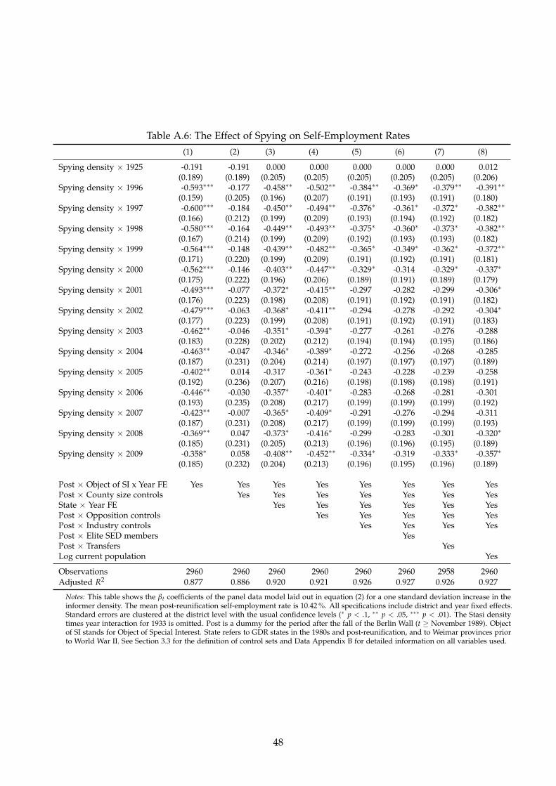
Table A.6: The Effect of Spying on Self-Employment Rates(1) (2) (3) (4) (5) (6) (7) (8)

Spying density × 1925 -0.191 -0.191 0.000 0.000 0.000 0.000 0.000 0.012(0.189) (0.189) (0.205) (0.205) (0.205) (0.205) (0.205) (0.206)

Spying density × 1996 -0.593∗∗∗ -0.177 -0.458∗∗ -0.502∗∗ -0.384∗∗ -0.369∗ -0.379∗∗ -0.391∗∗

(0.159) (0.205) (0.196) (0.207) (0.191) (0.193) (0.191) (0.180)Spying density × 1997 -0.600∗∗∗ -0.184 -0.450∗∗ -0.494∗∗ -0.376∗ -0.361∗ -0.372∗ -0.382∗∗

(0.166) (0.212) (0.199) (0.209) (0.193) (0.194) (0.192) (0.182)Spying density × 1998 -0.580∗∗∗ -0.164 -0.449∗∗ -0.493∗∗ -0.375∗ -0.360∗ -0.373∗ -0.382∗∗

(0.167) (0.214) (0.199) (0.209) (0.192) (0.193) (0.193) (0.182)Spying density × 1999 -0.564∗∗∗ -0.148 -0.439∗∗ -0.482∗∗ -0.365∗ -0.349∗ -0.362∗ -0.372∗∗

(0.171) (0.220) (0.199) (0.209) (0.191) (0.192) (0.191) (0.181)Spying density × 2000 -0.562∗∗∗ -0.146 -0.403∗∗ -0.447∗∗ -0.329∗ -0.314 -0.329∗ -0.337∗

(0.175) (0.222) (0.196) (0.206) (0.189) (0.191) (0.189) (0.179)Spying density × 2001 -0.493∗∗∗ -0.077 -0.372∗ -0.415∗∗ -0.297 -0.282 -0.299 -0.306∗

(0.176) (0.223) (0.198) (0.208) (0.191) (0.192) (0.191) (0.182)Spying density × 2002 -0.479∗∗∗ -0.063 -0.368∗ -0.411∗∗ -0.294 -0.278 -0.292 -0.304∗

(0.177) (0.223) (0.199) (0.208) (0.191) (0.192) (0.191) (0.183)Spying density × 2003 -0.462∗∗ -0.046 -0.351∗ -0.394∗ -0.277 -0.261 -0.276 -0.288

(0.183) (0.228) (0.202) (0.212) (0.194) (0.194) (0.195) (0.186)Spying density × 2004 -0.463∗∗ -0.047 -0.346∗ -0.389∗ -0.272 -0.256 -0.268 -0.285

(0.187) (0.231) (0.204) (0.214) (0.197) (0.197) (0.197) (0.189)Spying density × 2005 -0.402∗∗ 0.014 -0.317 -0.361∗ -0.243 -0.228 -0.239 -0.258

(0.192) (0.236) (0.207) (0.216) (0.198) (0.198) (0.198) (0.191)Spying density × 2006 -0.446∗∗ -0.030 -0.357∗ -0.401∗ -0.283 -0.268 -0.281 -0.301

(0.193) (0.235) (0.208) (0.217) (0.199) (0.199) (0.199) (0.192)Spying density × 2007 -0.423∗∗ -0.007 -0.365∗ -0.409∗ -0.291 -0.276 -0.294 -0.311

(0.187) (0.231) (0.208) (0.217) (0.199) (0.199) (0.199) (0.193)Spying density × 2008 -0.369∗∗ 0.047 -0.373∗ -0.416∗ -0.299 -0.283 -0.301 -0.320∗

(0.185) (0.231) (0.205) (0.213) (0.196) (0.196) (0.195) (0.189)Spying density × 2009 -0.358∗ 0.058 -0.408∗∗ -0.452∗∗ -0.334∗ -0.319 -0.333∗ -0.357∗

(0.185) (0.232) (0.204) (0.213) (0.196) (0.195) (0.196) (0.189)

Post × Object of SI x Year FE Yes Yes Yes Yes Yes Yes Yes YesPost × County size controls Yes Yes Yes Yes Yes Yes YesState × Year FE Yes Yes Yes Yes Yes YesPost × Opposition controls Yes Yes Yes Yes YesPost × Industry controls Yes Yes Yes YesPost × Elite SED members YesPost × Transfers YesLog current population Yes

Observations 2960 2960 2960 2960 2960 2960 2958 2960Adjusted R2 0.877 0.886 0.920 0.921 0.926 0.927 0.926 0.927

Notes: This table shows the βt coefficients of the panel data model laid out in equation (2) for a one standard deviation increase in theinformer density. The mean post-reunification self-employment rate is 10.42 %. All specifications include district and year fixed effects.Standard errors are clustered at the district level with the usual confidence levels (∗ p < .1, ∗∗ p < .05, ∗∗∗ p < .01). The Stasi densitytimes year interaction for 1933 is omitted. Post is a dummy for the period after the fall of the Berlin Wall (t ≥ November 1989). Objectof SI stands for Object of Special Interest. State refers to GDR states in the 1980s and post-reunification, and to Weimar provinces priorto World War II. See Section 3.3 for the definition of control sets and Data Appendix B for detailed information on all variables used.

48

Table A.7: The Effect of Spying on Unemployment Rates(1) (2) (3) (4) (5) (6) (7) (8)

Spying density × 1996 3.092∗∗∗ 0.538 0.872∗∗∗ 0.902∗∗∗ 0.916∗∗∗ 0.912∗∗∗ 0.924∗∗∗ 0.929∗∗∗

(0.431) (0.358) (0.324) (0.327) (0.337) (0.336) (0.337) (0.332)Spying density × 1997 2.907∗∗∗ 0.352 0.733∗∗ 0.763∗∗ 0.778∗∗ 0.773∗∗ 0.783∗∗ 0.789∗∗

(0.435) (0.365) (0.328) (0.332) (0.342) (0.340) (0.340) (0.336)Spying density × 1998 2.746∗∗∗ 0.192 0.467 0.498 0.512 0.507 0.512 0.524

(0.418) (0.365) (0.319) (0.322) (0.331) (0.330) (0.331) (0.324)Spying density × 1999 2.768∗∗∗ 0.214 0.399 0.430 0.444 0.439 0.444 0.457

(0.402) (0.355) (0.306) (0.312) (0.321) (0.319) (0.320) (0.313)Spying density × 2000 2.886∗∗∗ 0.332 0.499 0.529∗ 0.543∗ 0.538∗ 0.540∗ 0.557∗

(0.402) (0.356) (0.308) (0.315) (0.324) (0.323) (0.323) (0.318)Spying density × 2001 3.044∗∗∗ 0.490 0.572∗ 0.602∗ 0.617∗ 0.612∗ 0.612∗ 0.632∗

(0.401) (0.347) (0.312) (0.321) (0.331) (0.329) (0.331) (0.326)Spying density × 2002 2.985∗∗∗ 0.431 0.528∗ 0.558∗ 0.573∗ 0.568∗ 0.573∗ 0.590∗

(0.404) (0.347) (0.319) (0.329) (0.337) (0.335) (0.337) (0.331)Spying density × 2003 3.227∗∗∗ 0.673∗ 0.613∗ 0.643∗ 0.658∗ 0.653∗ 0.658∗ 0.678∗

(0.438) (0.367) (0.337) (0.345) (0.352) (0.350) (0.352) (0.348)Spying density × 2004 3.349∗∗∗ 0.795∗∗ 0.683∗∗ 0.713∗∗ 0.728∗∗ 0.723∗∗ 0.736∗∗ 0.750∗∗

(0.446) (0.376) (0.346) (0.354) (0.360) (0.359) (0.360) (0.357)Spying density × 2005 3.245∗∗∗ 0.691∗ 0.766∗∗ 0.796∗∗ 0.810∗∗ 0.806∗∗ 0.820∗∗ 0.836∗∗

(0.426) (0.366) (0.338) (0.348) (0.354) (0.353) (0.353) (0.350)Spying density × 2006 3.333∗∗∗ 0.779∗∗ 0.787∗∗ 0.817∗∗ 0.832∗∗ 0.827∗∗ 0.838∗∗ 0.860∗∗

(0.423) (0.370) (0.345) (0.354) (0.360) (0.358) (0.360) (0.359)Spying density × 2007 3.332∗∗∗ 0.778∗∗ 0.754∗∗ 0.784∗∗ 0.798∗∗ 0.794∗∗ 0.797∗∗ 0.830∗∗

(0.416) (0.368) (0.351) (0.360) (0.368) (0.366) (0.369) (0.366)Spying density × 2008 3.141∗∗∗ 0.586∗ 0.593∗ 0.623∗ 0.638∗ 0.633∗ 0.636∗ 0.673∗

(0.393) (0.351) (0.326) (0.336) (0.346) (0.344) (0.348) (0.344)Spying density × 2009 2.942∗∗∗ 0.387 0.567∗ 0.597∗ 0.611∗ 0.607∗ 0.632∗ 0.650∗

(0.377) (0.339) (0.321) (0.332) (0.343) (0.340) (0.343) (0.339)

Post × Object of SI x Year FE Yes Yes Yes Yes Yes Yes Yes YesPost × County size controls Yes Yes Yes Yes Yes Yes YesState × Year FE Yes Yes Yes Yes Yes YesPost × Opposition controls Yes Yes Yes Yes YesPost × Industry controls Yes Yes Yes YesPost × Elite SED members YesPost × Transfers YesLog current population Yes

Observations 2775 2775 2775 2775 2775 2775 2773 2775Adjusted R2 0.602 0.722 0.829 0.835 0.836 0.836 0.836 0.838

Notes: This table shows the βt coefficients of the panel data model laid out in equation (2) for a one standard deviation increase in the informerdensity. The mean post-reunification unemployment rate is 18.66 %. All specifications include district and year fixed effects. Standard errors areclustered at the district level with the usual confidence levels (∗ p < .1, ∗∗ p < .05, ∗∗∗ p < .01). The Stasi density times year interaction for 1933is omitted. Post is a dummy for the period after the fall of the Berlin Wall (t ≥ November 1989). Object of SI stands for Object of Special Interest.State refers to GDR states in the 1980s and post-reunification, and to Weimar provinces prior to World War II. See Section 3.3 for the definitionof control sets and Data Appendix B for detailed information on all variables used.

49

Table A.8: The Effect of Spying on Log Population(1) (2) (3) (4) (5) (6) (7)

Spying density × 1985 -0.001 -0.001 0.001 0.001 0.001 0.001 0.001(0.001) (0.001) (0.001) (0.001) (0.001) (0.001) (0.001)

Spying density × 1986 -0.000 -0.000 0.001 0.001 0.001 0.001 0.001(0.001) (0.001) (0.001) (0.001) (0.001) (0.001) (0.001)

Spying density × 1987 -0.000 -0.000 -0.000 -0.000 -0.000 -0.000 -0.000(0.000) (0.000) (0.000) (0.000) (0.000) (0.000) (0.000)

Spying density × 1989 0.002∗∗∗ -0.014∗∗∗ -0.013∗∗∗ -0.014∗∗∗ -0.013∗∗∗ -0.013∗∗∗ -0.012∗∗

(0.001) (0.003) (0.004) (0.004) (0.004) (0.004) (0.005)Spying density × 1990 0.004∗∗∗ -0.012∗∗∗ -0.012∗∗∗ -0.013∗∗∗ -0.012∗∗∗ -0.012∗∗∗

(0.001) (0.003) (0.004) (0.004) (0.004) (0.004)Spying density × 1991 0.003∗∗∗ -0.013∗∗∗ -0.013∗∗∗ -0.014∗∗∗ -0.013∗∗∗ -0.013∗∗∗

(0.001) (0.003) (0.004) (0.004) (0.004) (0.004)Spying density × 1992 0.004∗∗∗ -0.012∗∗∗ -0.012∗∗∗ -0.013∗∗∗ -0.012∗∗∗ -0.012∗∗∗

(0.001) (0.003) (0.004) (0.004) (0.004) (0.004)Spying density × 1993 0.004∗∗∗ -0.012∗∗∗ -0.012∗∗∗ -0.013∗∗∗ -0.012∗∗∗ -0.012∗∗∗

(0.002) (0.003) (0.004) (0.004) (0.004) (0.004)Spying density × 1994 0.006∗∗∗ -0.010∗∗∗ -0.012∗∗∗ -0.013∗∗∗ -0.012∗∗∗ -0.012∗∗∗

(0.002) (0.004) (0.004) (0.004) (0.004) (0.004)Spying density × 1995 0.008∗∗∗ -0.009∗∗ -0.011∗∗ -0.012∗∗∗ -0.012∗∗ -0.012∗∗ -0.015∗∗∗

(0.003) (0.004) (0.005) (0.004) (0.005) (0.005) (0.006)Spying density × 1996 0.010∗∗∗ -0.006 -0.011∗∗ -0.012∗∗ -0.011∗∗ -0.011∗∗ -0.014∗∗

(0.003) (0.004) (0.005) (0.005) (0.005) (0.005) (0.006)Spying density × 1997 0.013∗∗∗ -0.004 -0.010∗ -0.011∗ -0.010 -0.010 -0.014∗∗

(0.004) (0.005) (0.006) (0.006) (0.006) (0.006) (0.007)Spying density × 1998 0.014∗∗∗ -0.002 -0.011 -0.011∗ -0.011 -0.011 -0.014∗

(0.005) (0.006) (0.007) (0.007) (0.007) (0.007) (0.008)Spying density × 1999 0.016∗∗∗ -0.000 -0.011 -0.012 -0.011 -0.011 -0.015∗

(0.006) (0.006) (0.008) (0.008) (0.008) (0.008) (0.008)Spying density × 2000 0.017∗∗∗ 0.001 -0.012 -0.013 -0.012 -0.012 -0.016∗

(0.006) (0.007) (0.008) (0.008) (0.009) (0.009) (0.009)Spying density × 2001 0.017∗∗ 0.001 -0.013 -0.014 -0.013 -0.013 -0.017∗

(0.007) (0.007) (0.009) (0.009) (0.009) (0.009) (0.009)Spying density × 2002 0.017∗∗ 0.001 -0.014 -0.015 -0.014 -0.014 -0.018∗

(0.007) (0.008) (0.009) (0.009) (0.010) (0.010) (0.010)Spying density × 2003 0.017∗∗ 0.000 -0.016 -0.017∗ -0.016 -0.016 -0.020∗

(0.007) (0.008) (0.010) (0.010) (0.010) (0.010) (0.010)Spying density × 2004 0.016∗∗ 0.000 -0.017∗ -0.018∗ -0.017∗ -0.017∗ -0.021∗

(0.008) (0.008) (0.010) (0.010) (0.010) (0.010) (0.011)Spying density × 2005 0.016∗ -0.001 -0.019∗ -0.020∗ -0.019∗ -0.019∗ -0.023∗∗

(0.008) (0.009) (0.010) (0.010) (0.011) (0.011) (0.011)Spying density × 2006 0.015∗ -0.001 -0.021∗∗ -0.022∗∗ -0.022∗∗ -0.021∗ -0.025∗∗

(0.008) (0.009) (0.011) (0.011) (0.011) (0.011) (0.011)Spying density × 2007 0.015∗ -0.002 -0.023∗∗ -0.024∗∗ -0.024∗∗ -0.023∗∗ -0.027∗∗

(0.009) (0.009) (0.011) (0.011) (0.011) (0.011) (0.011)Spying density × 2008 0.014 -0.003 -0.026∗∗ -0.026∗∗ -0.026∗∗ -0.026∗∗ -0.030∗∗

(0.009) (0.009) (0.011) (0.011) (0.011) (0.011) (0.012)Spying density × 2009 0.013 -0.003 -0.028∗∗ -0.028∗∗ -0.028∗∗ -0.028∗∗ -0.030∗∗

(0.009) (0.010) (0.011) (0.011) (0.012) (0.012) (0.012)

Post × Object of SI x Year FE Yes Yes Yes Yes Yes Yes YesPost × County size controls Yes Yes Yes Yes Yes YesState × Year FE Yes Yes Yes Yes YesPost × Opposition controls Yes Yes Yes YesPost × Industry controls Yes Yes YesPost × Elite SED members YesPost × Transfers Yes

Observations 4625 4625 4625 4625 4625 4625 3698Adjusted R2 0.526 0.553 0.688 0.690 0.691 0.691 0.754

Notes: This table shows the βt coefficients of the panel data model laid out in equation (2) for a one standard deviation increasein the informer density. All specifications include district and year fixed effects. Standard errors are clustered at the district levelwith the usual confidence levels (∗ p < .1, ∗∗ p < .05, ∗∗∗ p < .01). The Stasi density times year interaction for 1988 is omitted. Postis a dummy for the period after the fall of the Berlin Wall (t ≥ November 1989). Object of SI stands for Object of Special Interest.State refers to GDR states in the 1980s and post-reunification, and to Weimar provinces prior to World War II. See Section 3.3 forthe definition of control sets and Data Appendix B for detailed information on all variables used.

50

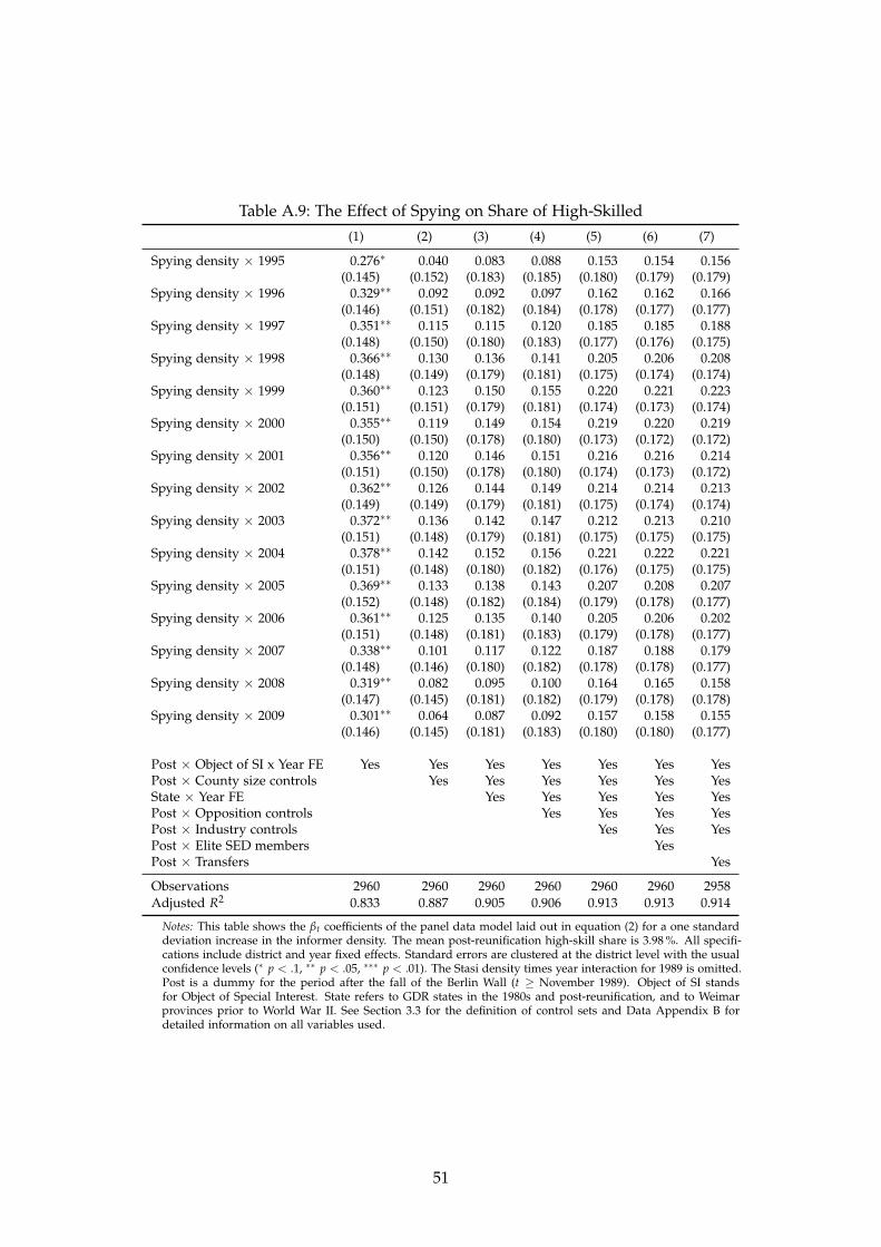
Table A.9: The Effect of Spying on Share of High-Skilled(1) (2) (3) (4) (5) (6) (7)

Spying density × 1995 0.276∗ 0.040 0.083 0.088 0.153 0.154 0.156(0.145) (0.152) (0.183) (0.185) (0.180) (0.179) (0.179)

Spying density × 1996 0.329∗∗ 0.092 0.092 0.097 0.162 0.162 0.166(0.146) (0.151) (0.182) (0.184) (0.178) (0.177) (0.177)

Spying density × 1997 0.351∗∗ 0.115 0.115 0.120 0.185 0.185 0.188(0.148) (0.150) (0.180) (0.183) (0.177) (0.176) (0.175)

Spying density × 1998 0.366∗∗ 0.130 0.136 0.141 0.205 0.206 0.208(0.148) (0.149) (0.179) (0.181) (0.175) (0.174) (0.174)

Spying density × 1999 0.360∗∗ 0.123 0.150 0.155 0.220 0.221 0.223(0.151) (0.151) (0.179) (0.181) (0.174) (0.173) (0.174)

Spying density × 2000 0.355∗∗ 0.119 0.149 0.154 0.219 0.220 0.219(0.150) (0.150) (0.178) (0.180) (0.173) (0.172) (0.172)

Spying density × 2001 0.356∗∗ 0.120 0.146 0.151 0.216 0.216 0.214(0.151) (0.150) (0.178) (0.180) (0.174) (0.173) (0.172)

Spying density × 2002 0.362∗∗ 0.126 0.144 0.149 0.214 0.214 0.213(0.149) (0.149) (0.179) (0.181) (0.175) (0.174) (0.174)

Spying density × 2003 0.372∗∗ 0.136 0.142 0.147 0.212 0.213 0.210(0.151) (0.148) (0.179) (0.181) (0.175) (0.175) (0.175)

Spying density × 2004 0.378∗∗ 0.142 0.152 0.156 0.221 0.222 0.221(0.151) (0.148) (0.180) (0.182) (0.176) (0.175) (0.175)

Spying density × 2005 0.369∗∗ 0.133 0.138 0.143 0.207 0.208 0.207(0.152) (0.148) (0.182) (0.184) (0.179) (0.178) (0.177)

Spying density × 2006 0.361∗∗ 0.125 0.135 0.140 0.205 0.206 0.202(0.151) (0.148) (0.181) (0.183) (0.179) (0.178) (0.177)

Spying density × 2007 0.338∗∗ 0.101 0.117 0.122 0.187 0.188 0.179(0.148) (0.146) (0.180) (0.182) (0.178) (0.178) (0.177)

Spying density × 2008 0.319∗∗ 0.082 0.095 0.100 0.164 0.165 0.158(0.147) (0.145) (0.181) (0.182) (0.179) (0.178) (0.178)

Spying density × 2009 0.301∗∗ 0.064 0.087 0.092 0.157 0.158 0.155(0.146) (0.145) (0.181) (0.183) (0.180) (0.180) (0.177)



Notes: This table shows the βt coefficients of the panel data model laid out in equation (2) for a one standarddeviation increase in the informer density. The mean post-reunification high-skill share is 3.98 %. All specifi-cations include district and year fixed effects. Standard errors are clustered at the district level with the usualconfidence levels (∗ p < .1, ∗∗ p < .05, ∗∗∗ p < .01). The Stasi density times year interaction for 1989 is omitted.Post is a dummy for the period after the fall of the Berlin Wall (t ≥ November 1989). Object of SI standsfor Object of Special Interest. State refers to GDR states in the 1980s and post-reunification, and to Weimarprovinces prior to World War II. See Section 3.3 for the definition of control sets and Data Appendix B fordetailed information on all variables used.

51

Table A.10: The Effect of Spying on Population Share below 15(1) (2) (3) (4) (5) (6) (7)

Spying density × 1990 -0.003 0.356∗∗∗ 0.025 0.029 0.039 0.039(0.047) (0.064) (0.072) (0.074) (0.073) (0.073)

Spying density × 1991 -0.022 0.338∗∗∗ 0.045 0.049 0.058 0.058(0.048) (0.058) (0.065) (0.067) (0.067) (0.067)

Spying density × 1992 -0.036 0.324∗∗∗ 0.068 0.072 0.081 0.081(0.052) (0.053) (0.060) (0.062) (0.062) (0.062)

Spying density × 1993 -0.071 0.289∗∗∗ 0.082 0.086 0.095∗ 0.095∗

(0.058) (0.048) (0.053) (0.055) (0.055) (0.055)Spying density × 1994 -0.114 0.246∗∗∗ 0.068 0.071 0.081 0.081

(0.069) (0.048) (0.051) (0.053) (0.052) (0.052)Spying density × 1995 -0.150∗ 0.209∗∗∗ 0.068 0.072 0.081 0.081 0.086

(0.080) (0.050) (0.050) (0.052) (0.050) (0.050) (0.056)Spying density × 1996 -0.171∗∗ 0.189∗∗∗ 0.080 0.084 0.093∗ 0.093∗ 0.095∗

(0.084) (0.049) (0.050) (0.052) (0.050) (0.050) (0.055)Spying density × 1997 -0.199∗∗ 0.160∗∗∗ 0.081 0.085∗ 0.094∗ 0.094∗ 0.097∗

(0.088) (0.048) (0.050) (0.051) (0.049) (0.049) (0.052)Spying density × 1998 -0.222∗∗ 0.137∗∗∗ 0.079 0.083 0.092∗ 0.092∗ 0.094∗

(0.091) (0.047) (0.050) (0.051) (0.050) (0.050) (0.051)Spying density × 1999 -0.258∗∗∗ 0.101∗∗ 0.069 0.072 0.082 0.082 0.084∗

(0.095) (0.048) (0.052) (0.053) (0.051) (0.051) (0.050)Spying density × 2000 -0.302∗∗∗ 0.057 0.054 0.058 0.067 0.067 0.071

(0.099) (0.049) (0.053) (0.054) (0.052) (0.052) (0.050)Spying density × 2001 -0.350∗∗∗ 0.010 0.029 0.033 0.042 0.042 0.049

(0.102) (0.050) (0.055) (0.055) (0.054) (0.054) (0.051)Spying density × 2002 -0.405∗∗∗ -0.046 -0.001 0.002 0.012 0.012 0.019

(0.105) (0.052) (0.056) (0.056) (0.055) (0.055) (0.052)Spying density × 2003 -0.453∗∗∗ -0.094∗ -0.030 -0.026 -0.016 -0.016 -0.007

(0.107) (0.052) (0.057) (0.057) (0.056) (0.056) (0.052)Spying density × 2004 -0.495∗∗∗ -0.135∗∗ -0.051 -0.047 -0.037 -0.037 -0.027

(0.110) (0.055) (0.059) (0.059) (0.059) (0.059) (0.054)Spying density × 2005 -0.523∗∗∗ -0.164∗∗∗ -0.067 -0.063 -0.053 -0.053 -0.043

(0.112) (0.057) (0.061) (0.060) (0.060) (0.060) (0.055)Spying density × 2006 -0.542∗∗∗ -0.183∗∗∗ -0.089 -0.085 -0.076 -0.075 -0.061

(0.112) (0.058) (0.061) (0.061) (0.061) (0.061) (0.055)Spying density × 2007 -0.562∗∗∗ -0.202∗∗∗ -0.113∗ -0.109∗ -0.099 -0.099 -0.080

(0.114) (0.060) (0.063) (0.063) (0.064) (0.064) (0.058)Spying density × 2008 -0.573∗∗∗ -0.213∗∗∗ -0.135∗∗ -0.131∗∗ -0.122∗ -0.122∗ -0.104∗

(0.114) (0.062) (0.065) (0.065) (0.065) (0.065) (0.060)Spying density × 2009 -0.583∗∗∗ -0.223∗∗∗ -0.153∗∗ -0.149∗∗ -0.140∗∗ -0.140∗∗ -0.105∗

(0.114) (0.063) (0.066) (0.066) (0.066) (0.066) (0.060)



Notes: This table shows the βt coefficients of the panel data model laid out in equation (2) for a one standard deviationincrease in the informer density. The mean post-reunification population share is 14.08 %. All specifications include districtand year fixed effects. Standard errors are clustered at the district level with the usual confidence levels (∗ p < .1, ∗∗ p < .05,∗∗∗ p < .01). The Stasi density times year interaction for 1989 is omitted. Post is a dummy for the period after the fall of theBerlin Wall (t ≥ November 1989). Object of SI stands for Object of Special Interest. State refers to GDR states in the 1980sand post-reunification, and to Weimar provinces prior to World War II. See Section 3.3 for the definition of control sets andData Appendix B for detailed information on all variables used.

52

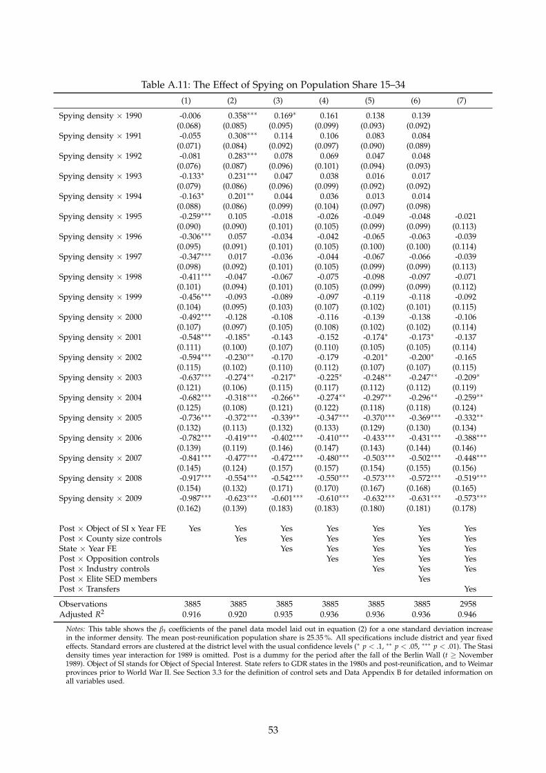
Table A.11: The Effect of Spying on Population Share 15–34(1) (2) (3) (4) (5) (6) (7)

Spying density × 1990 -0.006 0.358∗∗∗ 0.169∗ 0.161 0.138 0.139(0.068) (0.085) (0.095) (0.099) (0.093) (0.092)

Spying density × 1991 -0.055 0.308∗∗∗ 0.114 0.106 0.083 0.084(0.071) (0.084) (0.092) (0.097) (0.090) (0.089)

Spying density × 1992 -0.081 0.283∗∗∗ 0.078 0.069 0.047 0.048(0.076) (0.087) (0.096) (0.101) (0.094) (0.093)

Spying density × 1993 -0.133∗ 0.231∗∗∗ 0.047 0.038 0.016 0.017(0.079) (0.086) (0.096) (0.099) (0.092) (0.092)

Spying density × 1994 -0.163∗ 0.201∗∗ 0.044 0.036 0.013 0.014(0.088) (0.086) (0.099) (0.104) (0.097) (0.098)

Spying density × 1995 -0.259∗∗∗ 0.105 -0.018 -0.026 -0.049 -0.048 -0.021(0.090) (0.090) (0.101) (0.105) (0.099) (0.099) (0.113)

Spying density × 1996 -0.306∗∗∗ 0.057 -0.034 -0.042 -0.065 -0.063 -0.039(0.095) (0.091) (0.101) (0.105) (0.100) (0.100) (0.114)

Spying density × 1997 -0.347∗∗∗ 0.017 -0.036 -0.044 -0.067 -0.066 -0.039(0.098) (0.092) (0.101) (0.105) (0.099) (0.099) (0.113)

Spying density × 1998 -0.411∗∗∗ -0.047 -0.067 -0.075 -0.098 -0.097 -0.071(0.101) (0.094) (0.101) (0.105) (0.099) (0.099) (0.112)

Spying density × 1999 -0.456∗∗∗ -0.093 -0.089 -0.097 -0.119 -0.118 -0.092(0.104) (0.095) (0.103) (0.107) (0.102) (0.101) (0.115)

Spying density × 2000 -0.492∗∗∗ -0.128 -0.108 -0.116 -0.139 -0.138 -0.106(0.107) (0.097) (0.105) (0.108) (0.102) (0.102) (0.114)

Spying density × 2001 -0.548∗∗∗ -0.185∗ -0.143 -0.152 -0.174∗ -0.173∗ -0.137(0.111) (0.100) (0.107) (0.110) (0.105) (0.105) (0.114)

Spying density × 2002 -0.594∗∗∗ -0.230∗∗ -0.170 -0.179 -0.201∗ -0.200∗ -0.165(0.115) (0.102) (0.110) (0.112) (0.107) (0.107) (0.115)

Spying density × 2003 -0.637∗∗∗ -0.274∗∗ -0.217∗ -0.225∗ -0.248∗∗ -0.247∗∗ -0.209∗

(0.121) (0.106) (0.115) (0.117) (0.112) (0.112) (0.119)Spying density × 2004 -0.682∗∗∗ -0.318∗∗∗ -0.266∗∗ -0.274∗∗ -0.297∗∗ -0.296∗∗ -0.259∗∗

(0.125) (0.108) (0.121) (0.122) (0.118) (0.118) (0.124)Spying density × 2005 -0.736∗∗∗ -0.372∗∗∗ -0.339∗∗ -0.347∗∗∗ -0.370∗∗∗ -0.369∗∗∗ -0.332∗∗

(0.132) (0.113) (0.132) (0.133) (0.129) (0.130) (0.134)Spying density × 2006 -0.782∗∗∗ -0.419∗∗∗ -0.402∗∗∗ -0.410∗∗∗ -0.433∗∗∗ -0.431∗∗∗ -0.388∗∗∗

(0.139) (0.119) (0.146) (0.147) (0.143) (0.144) (0.146)Spying density × 2007 -0.841∗∗∗ -0.477∗∗∗ -0.472∗∗∗ -0.480∗∗∗ -0.503∗∗∗ -0.502∗∗∗ -0.448∗∗∗

(0.145) (0.124) (0.157) (0.157) (0.154) (0.155) (0.156)Spying density × 2008 -0.917∗∗∗ -0.554∗∗∗ -0.542∗∗∗ -0.550∗∗∗ -0.573∗∗∗ -0.572∗∗∗ -0.519∗∗∗

(0.154) (0.132) (0.171) (0.170) (0.167) (0.168) (0.165)Spying density × 2009 -0.987∗∗∗ -0.623∗∗∗ -0.601∗∗∗ -0.610∗∗∗ -0.632∗∗∗ -0.631∗∗∗ -0.573∗∗∗

(0.162) (0.139) (0.183) (0.183) (0.180) (0.181) (0.178)



Notes: This table shows the βt coefficients of the panel data model laid out in equation (2) for a one standard deviation increasein the informer density. The mean post-reunification population share is 25.35 %. All specifications include district and year fixedeffects. Standard errors are clustered at the district level with the usual confidence levels (∗ p < .1, ∗∗ p < .05, ∗∗∗ p < .01). The Stasidensity times year interaction for 1989 is omitted. Post is a dummy for the period after the fall of the Berlin Wall (t ≥ November1989). Object of SI stands for Object of Special Interest. State refers to GDR states in the 1980s and post-reunification, and to Weimarprovinces prior to World War II. See Section 3.3 for the definition of control sets and Data Appendix B for detailed information onall variables used.

53

Table A.12: The Effect of Spying on Population Share 35–54(1) (2) (3) (4) (5) (6) (7)

Spying density × 1990 0.111 -0.708∗∗∗ -0.428∗∗∗ -0.431∗∗∗ -0.369∗∗∗ -0.369∗∗∗

(0.070) (0.097) (0.124) (0.126) (0.127) (0.127)Spying density × 1991 0.132∗ -0.687∗∗∗ -0.398∗∗∗ -0.400∗∗∗ -0.338∗∗∗ -0.338∗∗∗

(0.072) (0.093) (0.120) (0.122) (0.123) (0.122)Spying density × 1992 0.159∗∗ -0.660∗∗∗ -0.373∗∗∗ -0.375∗∗∗ -0.313∗∗∗ -0.313∗∗∗

(0.075) (0.090) (0.114) (0.116) (0.117) (0.117)Spying density × 1993 0.208∗∗∗ -0.611∗∗∗ -0.341∗∗∗ -0.343∗∗∗ -0.281∗∗ -0.281∗∗

(0.078) (0.084) (0.107) (0.109) (0.110) (0.110)Spying density × 1994 0.305∗∗∗ -0.513∗∗∗ -0.283∗∗∗ -0.285∗∗∗ -0.223∗∗ -0.223∗∗

(0.087) (0.077) (0.097) (0.098) (0.100) (0.100)Spying density × 1995 0.364∗∗∗ -0.455∗∗∗ -0.290∗∗∗ -0.293∗∗∗ -0.231∗∗ -0.231∗∗ -0.345∗∗∗

(0.094) (0.073) (0.087) (0.088) (0.089) (0.089) (0.113)Spying density × 1996 0.442∗∗∗ -0.377∗∗∗ -0.248∗∗∗ -0.250∗∗∗ -0.188∗∗ -0.188∗∗ -0.302∗∗∗

(0.103) (0.072) (0.082) (0.083) (0.081) (0.081) (0.103)Spying density × 1997 0.527∗∗∗ -0.292∗∗∗ -0.199∗∗ -0.201∗∗ -0.139∗ -0.139∗ -0.254∗∗∗

(0.114) (0.075) (0.079) (0.080) (0.077) (0.077) (0.094)Spying density × 1998 0.640∗∗∗ -0.178∗∗ -0.132 -0.134 -0.072 -0.072 -0.188∗∗

(0.126) (0.079) (0.080) (0.081) (0.075) (0.075) (0.088)Spying density × 1999 0.763∗∗∗ -0.055 -0.073 -0.075 -0.013 -0.013 -0.129

(0.137) (0.086) (0.084) (0.085) (0.078) (0.078) (0.086)Spying density × 2000 0.871∗∗∗ 0.052 -0.023 -0.025 0.036 0.036 -0.082

(0.148) (0.094) (0.090) (0.090) (0.082) (0.082) (0.085)Spying density × 2001 0.991∗∗∗ 0.172∗ 0.033 0.030 0.092 0.092 -0.027

(0.156) (0.101) (0.097) (0.097) (0.088) (0.088) (0.086)Spying density × 2002 1.081∗∗∗ 0.262∗∗ 0.092 0.090 0.152 0.152 0.034

(0.164) (0.108) (0.103) (0.103) (0.094) (0.094) (0.089)Spying density × 2003 1.147∗∗∗ 0.328∗∗∗ 0.148 0.146 0.208∗∗ 0.208∗∗ 0.089

(0.169) (0.112) (0.110) (0.110) (0.100) (0.100) (0.093)Spying density × 2004 1.226∗∗∗ 0.407∗∗∗ 0.203∗ 0.200∗ 0.262∗∗ 0.262∗∗ 0.145

(0.176) (0.119) (0.119) (0.119) (0.110) (0.111) (0.101)Spying density × 2005 1.288∗∗∗ 0.469∗∗∗ 0.254∗∗ 0.252∗∗ 0.314∗∗∗ 0.314∗∗∗ 0.197∗

(0.181) (0.124) (0.126) (0.126) (0.118) (0.118) (0.106)Spying density × 2006 1.329∗∗∗ 0.511∗∗∗ 0.296∗∗ 0.294∗∗ 0.356∗∗∗ 0.356∗∗∗ 0.237∗∗

(0.184) (0.127) (0.131) (0.130) (0.122) (0.122) (0.110)Spying density × 2007 1.352∗∗∗ 0.534∗∗∗ 0.330∗∗ 0.328∗∗ 0.390∗∗∗ 0.390∗∗∗ 0.267∗∗

(0.184) (0.127) (0.134) (0.133) (0.127) (0.127) (0.116)Spying density × 2008 1.361∗∗∗ 0.542∗∗∗ 0.358∗∗∗ 0.356∗∗∗ 0.418∗∗∗ 0.418∗∗∗ 0.295∗∗

(0.185) (0.128) (0.137) (0.136) (0.129) (0.129) (0.118)Spying density × 2009 1.353∗∗∗ 0.534∗∗∗ 0.372∗∗∗ 0.370∗∗∗ 0.432∗∗∗ 0.432∗∗∗ 0.305∗∗

(0.184) (0.128) (0.140) (0.139) (0.132) (0.132) (0.123)



Notes: This table shows the βt coefficients of the panel data model laid out in equation (2) for a one standard deviation increasein the informer density. The mean post-reunification population share is 29.87 %. All specifications include district and year fixedeffects. Standard errors are clustered at the district level with the usual confidence levels (∗ p < .1, ∗∗ p < .05, ∗∗∗ p < .01). The Stasidensity times year interaction for 1989 is omitted. Post is a dummy for the period after the fall of the Berlin Wall (t ≥ November1989). Object of SI stands for Object of Special Interest. State refers to GDR states in the 1980s and post-reunification, and to Weimarprovinces prior to World War II. See Section 3.3 for the definition of control sets and Data Appendix B for detailed information onall variables used.

54

Table A.13: The Effect of Spying on Population Share above 54(1) (2) (3) (4) (5) (6) (7)

Spying density × 1990 -0.102 -0.006 0.234 0.241 0.192 0.191(0.135) (0.135) (0.155) (0.157) (0.157) (0.158)

Spying density × 1991 -0.055 0.040 0.239 0.246 0.197 0.196(0.135) (0.130) (0.149) (0.151) (0.152) (0.152)

Spying density × 1992 -0.042 0.054 0.228 0.234 0.185 0.184(0.137) (0.127) (0.144) (0.147) (0.147) (0.148)

Spying density × 1993 -0.004 0.092 0.213 0.219 0.171 0.169(0.140) (0.120) (0.134) (0.137) (0.137) (0.138)

Spying density × 1994 -0.029 0.066 0.172 0.178 0.130 0.128(0.154) (0.118) (0.134) (0.139) (0.139) (0.140)

Spying density × 1995 0.045 0.141 0.240∗∗ 0.247∗∗ 0.198∗ 0.197 0.280∗∗

(0.160) (0.122) (0.117) (0.122) (0.118) (0.119) (0.135)Spying density × 1996 0.035 0.131 0.201∗ 0.208∗ 0.159 0.158 0.246∗

(0.168) (0.122) (0.115) (0.120) (0.114) (0.115) (0.129)Spying density × 1997 0.020 0.115 0.154 0.161 0.112 0.111 0.196

(0.177) (0.125) (0.117) (0.122) (0.114) (0.115) (0.123)Spying density × 1998 -0.008 0.088 0.120 0.126 0.078 0.076 0.165

(0.187) (0.130) (0.122) (0.127) (0.118) (0.118) (0.121)Spying density × 1999 -0.049 0.047 0.093 0.100 0.051 0.050 0.138

(0.194) (0.135) (0.127) (0.132) (0.122) (0.122) (0.124)Spying density × 2000 -0.077 0.019 0.078 0.084 0.035 0.034 0.117

(0.199) (0.140) (0.131) (0.136) (0.125) (0.126) (0.125)Spying density × 2001 -0.093 0.003 0.082 0.088 0.040 0.038 0.115

(0.204) (0.143) (0.134) (0.139) (0.128) (0.128) (0.126)Spying density × 2002 -0.082 0.014 0.080 0.086 0.037 0.036 0.113

(0.209) (0.146) (0.137) (0.141) (0.131) (0.131) (0.128)Spying density × 2003 -0.056 0.039 0.098 0.105 0.056 0.055 0.127

(0.211) (0.147) (0.139) (0.143) (0.133) (0.134) (0.130)Spying density × 2004 -0.049 0.047 0.114 0.121 0.072 0.071 0.141

(0.214) (0.149) (0.142) (0.145) (0.137) (0.137) (0.133)Spying density × 2005 -0.029 0.067 0.152 0.159 0.110 0.109 0.177

(0.215) (0.152) (0.146) (0.149) (0.141) (0.142) (0.139)Spying density × 2006 -0.005 0.090 0.194 0.201 0.152 0.151 0.212

(0.219) (0.158) (0.153) (0.156) (0.149) (0.150) (0.148)Spying density × 2007 0.050 0.146 0.254 0.261 0.212 0.211 0.261

(0.220) (0.161) (0.159) (0.162) (0.158) (0.159) (0.159)Spying density × 2008 0.129 0.225 0.319∗ 0.326∗ 0.277 0.276 0.329∗

(0.226) (0.168) (0.168) (0.170) (0.168) (0.169) (0.167)Spying density × 2009 0.217 0.313∗ 0.383∗∗ 0.389∗∗ 0.341∗ 0.339∗ 0.373∗∗

(0.231) (0.174) (0.177) (0.179) (0.178) (0.179) (0.179)



Notes: This table shows the βt coefficients of the panel data model laid out in equation (2) for a one standard deviationincrease in the informer density. The mean post-reunification population share is 30.70 %. All specifications includedistrict and year fixed effects. Standard errors are clustered at the district level with the usual confidence levels (∗

p < .1, ∗∗ p < .05, ∗∗∗ p < .01). The Stasi density times year interaction for 1989 is omitted. Post is a dummy for theperiod after the fall of the Berlin Wall (t ≥ November 1989). Object of SI stands for Object of Special Interest. Staterefers to GDR states in the 1980s and post-reunification, and to Weimar provinces prior to World War II. See Section3.3 for the definition of control sets and Data Appendix B for detailed information on all variables used.

55

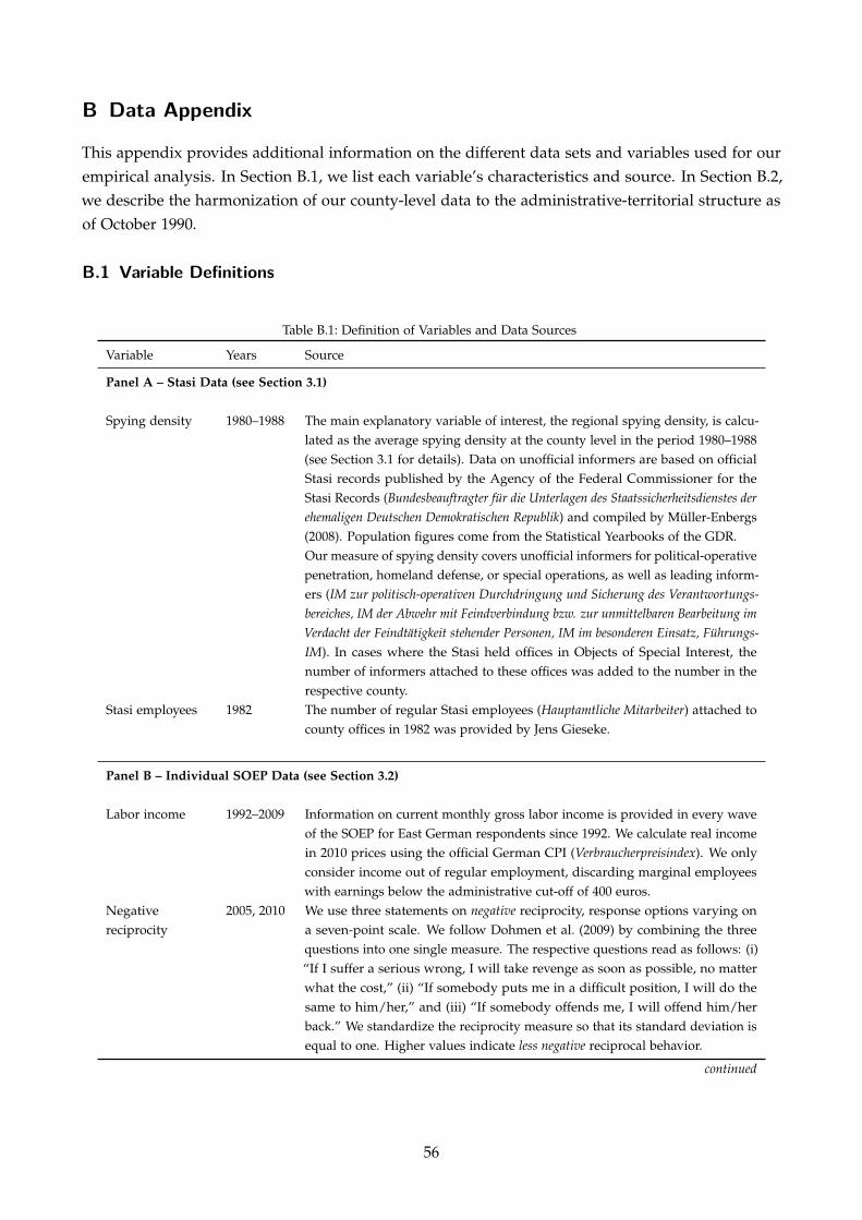
B Data Appendix

This appendix provides additional information on the different data sets and variables used for ourempirical analysis. In Section B.1, we list each variable’s characteristics and source. In Section B.2,we describe the harmonization of our county-level data to the administrative-territorial structure asof October 1990.

B.1 Variable Definitions

Table B.1: Definition of Variables and Data Sources

Variable Years Source

Panel A – Stasi Data (see Section 3.1)

Spying density 1980–1988 The main explanatory variable of interest, the regional spying density, is calcu-lated as the average spying density at the county level in the period 1980–1988(see Section 3.1 for details). Data on unofficial informers are based on officialStasi records published by the Agency of the Federal Commissioner for theStasi Records (Bundesbeauftragter fur die Unterlagen des Staatssicherheitsdienstes derehemaligen Deutschen Demokratischen Republik) and compiled by Muller-Enbergs(2008). Population figures come from the Statistical Yearbooks of the GDR.Our measure of spying density covers unofficial informers for political-operativepenetration, homeland defense, or special operations, as well as leading inform-ers (IM zur politisch-operativen Durchdringung und Sicherung des Verantwortungs-bereiches, IM der Abwehr mit Feindverbindung bzw. zur unmittelbaren Bearbeitung imVerdacht der Feindtatigkeit stehender Personen, IM im besonderen Einsatz, Fuhrungs-IM). In cases where the Stasi held offices in Objects of Special Interest, thenumber of informers attached to these offices was added to the number in therespective county.

Stasi employees 1982 The number of regular Stasi employees (Hauptamtliche Mitarbeiter) attached tocounty offices in 1982 was provided by Jens Gieseke.

Panel B – Individual SOEP Data (see Section 3.2)

Labor income 1992–2009 Information on current monthly gross labor income is provided in every waveof the SOEP for East German respondents since 1992. We calculate real incomein 2010 prices using the official German CPI (Verbraucherpreisindex). We onlyconsider income out of regular employment, discarding marginal employeeswith earnings below the administrative cut-off of 400 euros.

Negativereciprocity

2005, 2010 We use three statements on negative reciprocity, response options varying ona seven-point scale. We follow Dohmen et al. (2009) by combining the threequestions into one single measure. The respective questions read as follows: (i)“If I suffer a serious wrong, I will take revenge as soon as possible, no matterwhat the cost,” (ii) “If somebody puts me in a difficult position, I will do thesame to him/her,” and (iii) “If somebody offends me, I will offend him/herback.” We standardize the reciprocity measure so that its standard deviation isequal to one. Higher values indicate less negative reciprocal behavior.

continued

56

Table B.1 continued


Number of closefriends

2003, 2008 The underlying question reads as follows: “What would you say: How manyclose friends do you have?” We drop respondents that indicate implausiblehigh numbers of close friends (more than 15), which is equivalent to 0.9% ofthe sample, or 19 observations.

Participation in lo-cal politics

2001, 2007 Respondents are questioned about their involvement in citizen’s groups, politi-cal parties and local governments (the question reads: “Which of the followingactivities do you take part in during your free time?”). Response options varyon a four point scale indicating weekly, monthly, less often or no involvement atall. We construct a zero/one dummy variable indicating whether respondentsare involved (weekly, monthly, less often), or not.

Sociability 2005, 2009 The statement reads as follows: “I see myself as someone who is outgoing,sociable”. Response options were given on a seven-point scale to allow respon-dents to express different levels of conviction. We standardize the variable bydividing it by its standard deviation.

Trust in strangers 2003, 2008 The question on interpersonal trust reads as follows: “If one is dealing withstrangers, it is better to be careful before one can trust them.” Response optionswere given on a four-point scale, allowing the respondents to totally or slightlyagree, or totally or slightly disagree with the given statements. FollowingGlaeser et al. (2000), we define a dichotomous variable by grouping the formerand latter two answers.

Volunteering inclubs

2001, 2007 Respondents were questioned about their volunteering activities in clubs orsocial services (the question reads: “Which of the following activities do youtake part in during your free time?”). Response options vary on a four pointscale indicating weekly, monthly, less often or no involvement at all. Weconstruct a zero/one dummy variable indicating whether respondents areinvolved (weekly, monthly, less often), or not.

Control variables The set of control variables includes information on the respondents’ age, sex,household size, marital status, education and learned profession.

Panel C – County-Level Data (see Section 3.3)

County size 1990 The area of each East German county is reported in Rudolph (1990).Demographics 1989 Information on age-specific population shares are obtained from infas (n.d.).

1990–2009 Collected from the Statistical Offices of the Federal States (Statistische Lan-desamter) and the Regional Database Germany (Regionaldatenbank Deutschland).

Election turnout 1928–1932 We use election turnout in the federal elections in the Weimar Republic in 1928,1930, 07/1932 and 11/1932. The data is provided in the replication data of Kinget al. (2008), available at the Harvard Dataverse, handle: hdl/1902.1/11193.

Industry controls 1989 Information on the goods value of production is collected from infas (n.d.). Dataon the industrial composition of the workforce as of September 1989 is reportedin Rudolph (1990). We further collect information from various sources whetherlarge enterprises from the uranium, coal, potash, oil or chemical industry werelocated in the respective county. We construct a zero/one dummy based on thisdata.

continued

57

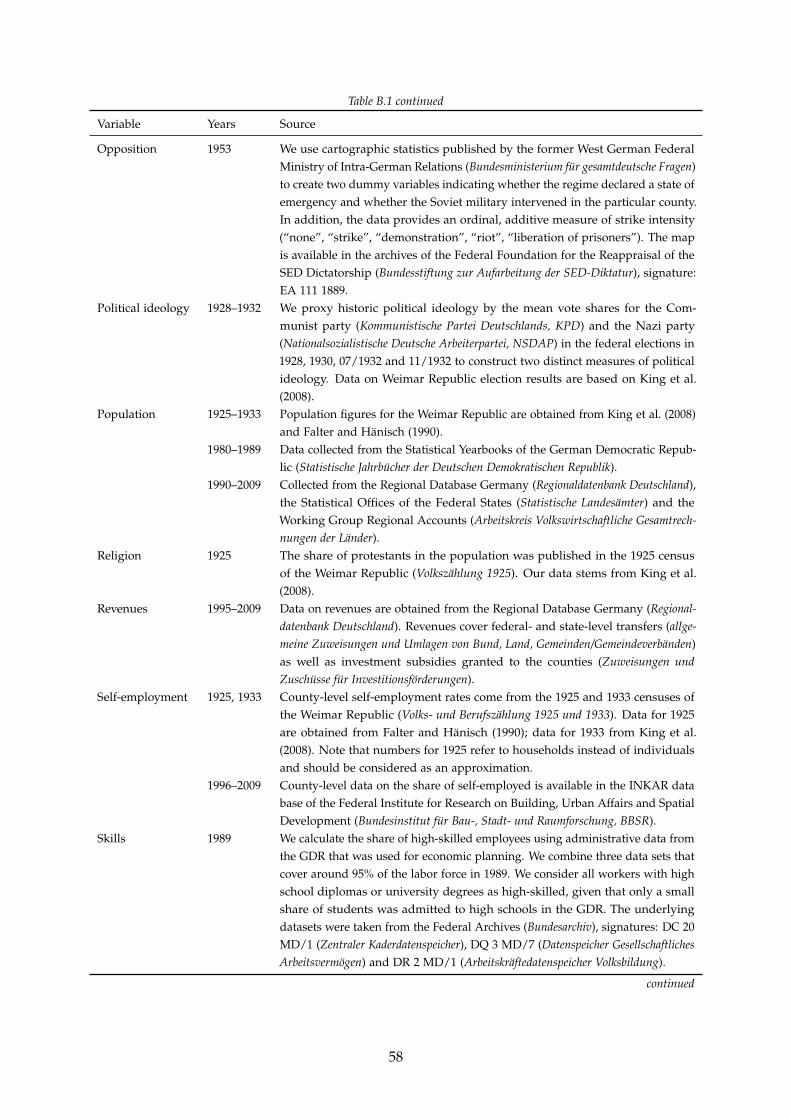
Table B.1 continued


Opposition 1953 We use cartographic statistics published by the former West German FederalMinistry of Intra-German Relations (Bundesministerium fur gesamtdeutsche Fragen)to create two dummy variables indicating whether the regime declared a state ofemergency and whether the Soviet military intervened in the particular county.In addition, the data provides an ordinal, additive measure of strike intensity(“none”, “strike”, “demonstration”, “riot”, “liberation of prisoners”). The mapis available in the archives of the Federal Foundation for the Reappraisal of theSED Dictatorship (Bundesstiftung zur Aufarbeitung der SED-Diktatur), signature:EA 111 1889.

Political ideology 1928–1932 We proxy historic political ideology by the mean vote shares for the Com-munist party (Kommunistische Partei Deutschlands, KPD) and the Nazi party(Nationalsozialistische Deutsche Arbeiterpartei, NSDAP) in the federal elections in1928, 1930, 07/1932 and 11/1932 to construct two distinct measures of politicalideology. Data on Weimar Republic election results are based on King et al.(2008).

Population 1925–1933 Population figures for the Weimar Republic are obtained from King et al. (2008)and Falter and Hanisch (1990).

1980–1989 Data collected from the Statistical Yearbooks of the German Democratic Repub-lic (Statistische Jahrbucher der Deutschen Demokratischen Republik).

1990–2009 Collected from the Regional Database Germany (Regionaldatenbank Deutschland),the Statistical Offices of the Federal States (Statistische Landesamter) and theWorking Group Regional Accounts (Arbeitskreis Volkswirtschaftliche Gesamtrech-nungen der Lander).

Religion 1925 The share of protestants in the population was published in the 1925 censusof the Weimar Republic (Volkszahlung 1925). Our data stems from King et al.(2008).

Revenues 1995–2009 Data on revenues are obtained from the Regional Database Germany (Regional-datenbank Deutschland). Revenues cover federal- and state-level transfers (allge-meine Zuweisungen und Umlagen von Bund, Land, Gemeinden/Gemeindeverbanden)as well as investment subsidies granted to the counties (Zuweisungen undZuschusse fur Investitionsforderungen).

Self-employment 1925, 1933 County-level self-employment rates come from the 1925 and 1933 censuses ofthe Weimar Republic (Volks- und Berufszahlung 1925 und 1933). Data for 1925are obtained from Falter and Hanisch (1990); data for 1933 from King et al.(2008). Note that numbers for 1925 refer to households instead of individualsand should be considered as an approximation.

1996–2009 County-level data on the share of self-employed is available in the INKAR database of the Federal Institute for Research on Building, Urban Affairs and SpatialDevelopment (Bundesinstitut fur Bau-, Stadt- und Raumforschung, BBSR).

Skills 1989 We calculate the share of high-skilled employees using administrative data fromthe GDR that was used for economic planning. We combine three data sets thatcover around 95% of the labor force in 1989. We consider all workers with highschool diplomas or university degrees as high-skilled, given that only a smallshare of students was admitted to high schools in the GDR. The underlyingdatasets were taken from the Federal Archives (Bundesarchiv), signatures: DC 20MD/1 (Zentraler Kaderdatenspeicher), DQ 3 MD/7 (Datenspeicher GesellschaftlichesArbeitsvermogen) and DR 2 MD/1 (Arbeitskraftedatenspeicher Volksbildung).

continued

58

Table B.1 continued


We replicate our analysis in Section 6.3 using alternative pre-reunification dataon the county-level skill distribution in large public companies provided bythe Statistical Offices of the East German Lander (Gemeinsames Statistisches Amtin Berlin, Regionalstatistische Angaben 1989 in der Gliederung nach Kreisen in denGrenzen der Lander, 1990, pp. 15–21). The results are very similar when usingthis alternative measure of skills.

1995–2009 The share of high-skilled employees in the working-age population is takenfrom the INKAR data base of the Federal Institute for Research on Building,Urban Affairs and Spatial Development (Bundesinstitut fur Bau-, Stadt- undRaumforschung, BBSR).

Socialistindoctrination

1988 We proxy regional socialist indoctrination by the share of political and economicelites that were members of the Socialist Unity Party (SED). We calculate thismeasure using data from the Central Cadre Database (Zentraler Kaderdatenspe-icher, ZKDS). This large administrative data set was used for planning purposesand contains information on all political and economic executives of the GDR(except for employees of the Ministry for State Security, the Ministry of NationalDefence and the Ministry of Internal Affairs). The data set is taken from theFederal Archives (Bundesarchiv), signature: DC 20 MD/1.

Unemployment 1933 County-level unemployment rates are based on the 1933 census of the WeimarRepublic (Volks- und Berufszahlung 1933), provided in King et al. (2008).

1996–2009 Monthly county-level unemployment rates are made available from March 1996to December 2009 by the Federal Employment Agency (Bundesagentur fur Arbeit).We calculate yearly means from this data.

59

B.2 Redrawn County Boundaries and Data Harmonization

We combine county-level data from various sources and decades in this study. Since 1924, the firstdata year in our analysis, county borders have been redrawn multiple times. To account for theseterritorial changes, we harmonize all county-level data to boundaries as of October 1990. Note thatthis procedure only applies to county-level measures and is not necessary in the SOEP data as weselect individuals based on their county of residence in 1990 and track these people over time.

The number of East German counties was gradually reduced from 216 at the time of the reunifi-cation to 87 in 2009. To keep track of changing county boundaries from 1991 onwards, we rely ondetailed population weighting matrices provided by the Federal Institute for Research on Building,Urban Affairs and Spatial Development (BBSR). Based on these weighting factors, we can calculatecounty-level measures (election turnout, self-employment rates, population figures, etc.) assumingcounterfactual county borders.

There were only minor territorial reforms during the existence of the GDR (more specificallybetween 1953–1990, the period for which we have data). In ten cases, neighboring counties weremerged together. In five cases, bigger cities became independent from the surrounding rural county(Stadtkreise). We manually account for these administrative changes using detailed maps and otherhistorical sources. When merging two counties, we always use the maximum for each of the threeopposition variables (state of emergency, Soviet military intervention, strike intensity). In case newcounties were constituted, we assign historical values of the emitting county to the created one.

When harmonizing data from the Weimar Republic with 1990 county boundaries, greater territorialreforms have to be taken into account. Due to the lack of adequate population weighting factors,the harmonization is based on geospatial area weighting factors as described in Goodchild and Lam(1980). We overlay the corresponding GIS shapefiles from the Weimar Republic with the shapefilefrom 1990 and calculate area weighting factors that allow for adjusting the historical data to countyborders as of 1990. MPIDR and CGG, 2011, provide a rich set of historical shapefiles for the Germanterritory. Given that most of our outcomes and control variables refer to people and not space, itneeds to be stressed that this procedure is afflicted with some degree of imprecision. Given thelong time span, the numerous territorial reforms, and the lack of population weighting factors, thisprocedure is, however, the most accurate harmonization procedure we can apply.

60

The Long-Term Costs of Government Surveillance: Insights ... · SOEPpapers on Multidisciplinary...

Documents

Transcript of The Long-Term Costs of Government Surveillance: Insights ... · SOEPpapers on Multidisciplinary...