The Location of Foreign Direct Investment in Chinese … Location of Foreign Direct Investment in...

This PDF is a selection from an out-of-print volume from the National Bureauof Economic Research

Volume Title: The Role of Foreign Direct Investment in East Asian EconomicDevelopment, NBER-EASE Volume 9

Volume Author/Editor: Takatoshi Ito and Anne O. Krueger, editors

Volume Publisher: University of Chicago Press

Volume ISBN: 0-226-38675-9

Volume URL: http://www.nber.org/books/ito_00-2

Conference Date: June 25-27, 1998

Publication Date: January 2000

Chapter Title: The Location of Foreign Direct Investment in Chinese Regions:Further Analysis of Labor Quality

Chapter Author: Leonard Cheng, Yum K. Kwan

Chapter URL: http://www.nber.org/chapters/c8500

Chapter pages in book: (p. 213 - 238)

The Location of Foreign Direct Investment in Chinese Regions Further Analysis of Labor Quality

Leonard K. Cheng and Yum K. Kwan

7.1 Introduction

Cross-border investment by multinational firms is one of the most salient features of today’s global economy, and many countries see attracting foreign direct investment (FDI) as an important element in their strategy for economic development. In this paper, we extend our earlier work (Cheng and Kwan 1999b), which attempted to uncover the factors that attract FDI based on the Chinese experience, by using a set of different proxies for labor quality. The Chinese experience with FDI is interesting for several reasons. First, China emerged as the largest recipient of FDI among developing countries beginning in 1992, and it has been the second largest recipient in the world (after the United States) since 1993. Second, unlike the United States and other developed economies, China has explicit policies to encourage the “export processing”-type FDI and has set up different economic zones for foreign investors.’ Third, the most important source economies investing in China (i.e., Hong Kong and Taiwan) are close to some provinces but not to others. In contrast, Western Europe and Japan, the most important sources of FDI for the United States, are not particularly close to any of the American states.

Leonard K. Cheng is professor of economics at the Hong Kong University of Science and Technology. Yum K. Kwan is associate professor of economics and finance at the City University of Hong Kong.

The authors thank Gregory Chow for suggesting the partial stock adjustment approach adopted in this paper, and Anne Krueger, Shang-Jin Wei, Laixun Zhao, and an anonymous referee for their helpful comments and suggestions. The work described in this paper was substantially supported by a grant from the Research Grant Council of the Hong Kong Special Administrative Region, China (Project no. HKUST484/94H).

1. Until the early 1990s, the Chinese domestic market was not open to foreign firms in China.

213

214 Leonard K. Cheng and Yum K. Kwan

The Chinese experience is an important case in the study of FDI, partly because of the sheer magnitude and fast growth of FDI the country has received in such a short period of time, but more importantly because of the diversity of the data. Due to changes in policies toward FDI and the occurrence of major economic and political events that caused changes in FDI flows, the Chinese case also serves as a natural experiment for us to test hypotheses about the incidence of FDI. We believe that the test results are not only relevant to China but also important in understanding the determinants of the location of FDI in general.

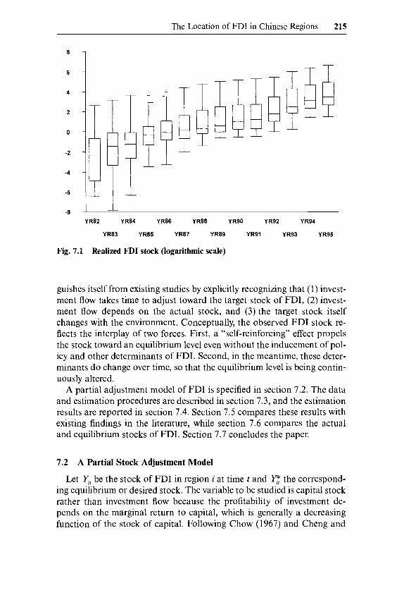
Figure 7.1 summarizes the Chinese data on regional FDI stocks by box plots.' Each box presents succinctly the regional distribution of the stocks in a given year; and the chronologically juxtaposed boxes reveal the time- series aspects of the data, in particular, the persistence of the median stock and the temporal variations of the regional distribution. The figure clearly shows that the location of FDI in China is characterized by enormous spatial as well as temporal diversity. A satisfactory empirical model must be able to explain these salient features in a consistent framework.

Potential determinants of FDI location have been extensively studied in the l i terat~re .~ The typical approach is to regress the chosen dependent variable, such as the probability of locating FDI in a location or the amount of investment in a location, on a set of independent variables that on theoretical grounds would likely affect the profitability of investment. These variables typically reflect or affect local market potential, cost of production, cost of transport, taxes, and the general business environment faced by foreign firms. In contrast with the bulk of the existing literature that is based on a comparative statics theory of FDI location, some recent papers have emphasized the importance of the self-perpetuating growth of FDI over time (including the agglomeration effect). They include Smith and Florida (1994), Head et al. (1995), 0 Huallachain and Reid (1997), and Cheng and Kwan (1999a, 1999b).

As an extension of our earlier work (1999b), the present paper distin-

2. As will be explained in section 7.3 below, the stock of FDI is taken to be the sum of FDI flows since 1979, where FDI flows are measured in constant U.S. dollars. The box plot summarizes a distribution by the median (the horizontal line within the box), the lower and upper quartiles (the two edges of the box), the extreme values (the two whiskers extending from the box), and outliers (points beyond the whiskers).

3. Reflecting U.S. leadership in both inward and outward FDI, the existing literature has focused on the geographical distribution of FDI in the United States as well as the location of U.S. direct investment in other countries. Recent studies include Coughlin, Terza, and Arromdee (1991), Friedman, Gerlowski, and Silberman (1992), Wheeler and Mody (1992), Woodward (1992), Smith and Florida (1994), Head, Ries, and Swenson (1995), Friedman et al. (1996), Hines (1996), and 0 Huallachain and Reid (1997). Hill and Munday (1995) studied the locational determinants of FDI in France and the United Kingdom. Rozelle, ying, and Barlow (n.d.), Cheng and Zhao (1995), Chen (1996), Head and Ries (1996), and Cheng and Kwan (1999a, 1999b) examined the case of China.

The Location of FDI in Chinese Regions 215

6 ,TT

Fig. 7.1 Realized FDI stock (logarithmic scale)

guishes itself from existing studies by explicitly recognizing that (1) investment flow takes time to adjust toward the target stock of FDI, (2) investment flow depends on the actual stock, and (3) the target stock itself changes with the environment. Conceptually, the observed FDI stock reflects the interplay of two forces. First, a “self-reinforcing’’ effect propels the stock toward an equilibrium level even without the inducement of policy and other determinants of FDI. Second, in the meantime, these determinants do change over time, so that the equilibrium level is being contin- uously altered.

A partial adjustment model of FDI is specified in section 7.2. The data and estimation procedures are described in section 7.3, and the estimation results are reported in section 7.4. Section 7.5 compares these results with existing findings in the literature, while section 7.6 compares the actual and equilibrium stocks of FDI. Section 7.7 concludes the paper.

7.2 A Partial Stock Adjustment Model

Let yr be the stock of FDI in region i at time t and the corresponding equilibrium or desired stock. The variable to be studied is capital stock rather than investment flow because the profitability of investment depends on the marginal return to capital, which is generally a decreasing function of the stock of capital. Following Chow (1967) and Cheng and


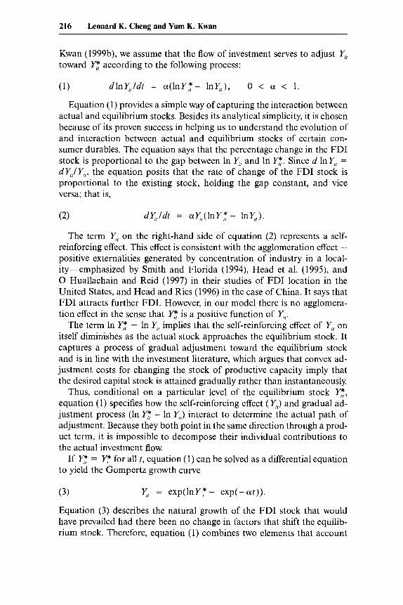
Kwan (1999b), we assume that the flow of investment serves to adjust Y,, toward c according to the following process:

(1) dlnqt/dt = a(lnY3- lnq,), 0 < a < 1

Equation (1) provides a simple way of capturing the interaction between actual and equilibrium stocks. Besides its analytical simplicity, it is chosen because of its proven success in helping us to understand the evolution of and interaction between actual and equilibrium stocks of certain consumer durables. The equation says that the percentage change in the FDI stock is proportional to the gap between In Y,, and In Y:. Since d lnY,, =

dy,/Y, , , the equation posits that the rate of change of the FDI stock is proportional to the existing stock, holding the gap constant, and vice versa; that is,

(2) dy , /d t = a ~ , ( l n Y ~ - lnq,).

The term Y,, on the right-hand side of equation (2) represents a self- reinforcing effect. This effect is consistent with the agglomeration effect- positive externalities generated by concentration of industry in a local- ity-emphasized by Smith and Florida (1994), Head et al. (1995), and 0 Huallachain and Reid (1997) in their studies of FDI location in the United States, and Head and Ries (1996) in the case of China. It says that FDI attracts further FDI. However, in our model there is no agglomeration effect in the sense that y1": is a positive function of Y,,.

The term In c - In Y,, implies that the self-reinforcing effect of Y,, on itself diminishes as the actual stock approaches the equilibrium stock. It captures a process of gradual adjustment toward the equilibrium stock and is in line with the investment literature, which argues that convex adjustment costs for changing the stock of productive capacity imply that the desired capital stock is attained gradually rather than instantaneously.

Thus, conditional on a particular level of the equilibrium stock c, equation (1) specifies how the self-reinforcing effect (YJ and gradual adjustment process (In - In Y,,) interact to determine the actual path of adjustment. Because they both point in the same direction through a prod- uct term, it is impossible to decompose their individual contributions to the actual investment flow.

If Y: = yI* for all t, equation (1) can be solved as a differential equation to yield the Gompertz growth curve

(3) qL = exp(lnY,*- exp(-aut)).

Equation (3) describes the natural growth of the FDI stock that would have prevailed had there been no change in factors that shift the equilibrium stock. Therefore, equation (1) combines two elements that account


for the observed accumulation of FDI. First, the self-reinforcing effect and the adjustment effect drive the FDI stock to an equilibrium level, and second, the equilibrium level itself shifts as a result of changes in the environment.

In empirical applications, equation (1) is replaced by its discrete version (where lowercase letters stand for logarithmic values, e.g., y,, = In YJ,

which, after collecting terms, becomes

For the adjustment process described by equation (5) to be nonexplo- sive and nonfluctuating, 1 - (Y must be a positive fraction. To estimate the above equation, we need to specify the determinants of y,T. Theoretically, the location choice of FDI is determined by relative profitability. If a location is chosen as the destination of FDI, then from the investor’s point of view, it must be more profitable to produce in that location than in others, given the location choice of other investors. If the goods are produced for export, the costs of producing the goods and the costs and reliability of transporting them to the world market are most crucial. If the goods and services are produced for the local market, then local demand factors would also matter. In both cases, government policies such as preferential tax treatment, the time and effort needed to gain government approval, the environment for doing business, and so forth, would affect a location’s attractiveness to foreign investor^.^ Depending on the relative importance of export-oriented and domestic-market-oriented FDI, however, the importance of the same determinants of FDI may vary.

Since FDI in China was primarily in the form of new plants, we focus on the statistical analysis of the location choice of greenfield FDI in the literature. Consistent with the theoretical considerations and empirical observations mentioned above, the existing literature has pointed to the importance of five sets of variabled

4. A general empirical observation is that export-oriented FDI is more responsive to preferential tax treatment, but FDI that is aimed at the local market is more responsive to policies on market access and policies that affect domestic demand. The Organization for Eco- nomic Cooperation and Development has stated that “one factor influencing the role played by investment incentives is whether the foreign investment is intended to replace imports by local production or is geared to production for export. In the former case, it is likely that the effect of incentives will be relatively limited. The existence of a specific and often pro- tected market is often the major determinant of the investment, as market protection is a powerful incentive. In the second case, on the other hand, incentives are probably more important” (OECD 1992, 81).

5. See the references cited in n. 3.


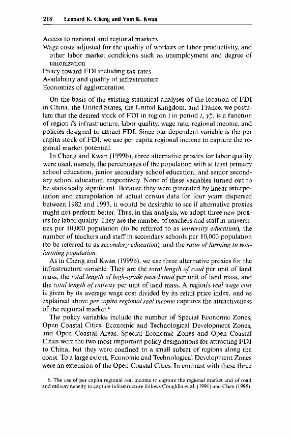
Access to national and regional markets Wage costs adjusted for the quality of workers or labor productivity, and

other labor market conditions such as unemployment and degree of unionization

Policy toward FDI including tax rates Availability and quality of infrastructure Economies of agglomeration

On the basis of the existing statistical analyses of the location of FDI in China, the United States, the United Kingdom, and France, we postulate that the desired stock of FDI in region i in period t , y,T, is a function of region i’s infrastructure, labor quality, wage rate, regional income, and policies designed to attract FDI. Since our dependent variable is the per capita stock of FDI, we use per capita regional income to capture the regional market potential.

In Cheng and Kwan (1999b), three alternative proxies for labor quality were used, namely, the percentages of the population with at least primary school education, junior secondary school education, and senior secondary school education, respectively. None of these variables turned out to be statistically significant. Because they were generated by linear interpo- lation and extrapolation of actual census data for four years dispersed between 1982 and 1993, it would be desirable to see if alternative proxies might not perform better. Thus, in this analysis, we adopt three new proxies for labor quality. They are the number of teachers and staff in universities per 10,000 population (to be referred to as university education), the number of teachers and staff in secondary schools per 10,000 population (to be referred to as secondary education), and the ratio of farming to nonfarming population.

As in Cheng and Kwan (1999b), we use three alternative proxies for the infrastructure variable. They are the total length of road per unit of land mass, the total length of high-grade paved road per unit of land mass, and the total length of railway per unit of land mass. A region’s real wage cost is given by its average wage cost divided by its retail price index, and as explained above per capita regional real income captures the attractiveness of the regional market.h

The policy variables include the number of Special Economic Zones, Open Coastal Cities, Economic and Technological Development Zones, and Open Coastal Areas. Special Economic Zones and Open Coastal Cities were the two most important policy designations for attracting FDI to China, but they were confined to a small subset of regions along the coast. To a large extent, Economic and Technological Development Zones were an extension of the Open Coastal Cities. In contrast with these three

6. The use of per capita regional real income to capture the regional market and of road and railway density to capture infrastructure follows Coughlin et al. (1991) and Chen (1996).


policy designations, Open Coastal Areas were introduced later, were far more numerous, and were geographically the most dispersed. In terms of the benefits provided by these policy designations, Special Economic Zones were clearly at the top, followed by Open Coastal Cities and Eco- nomic and Technological Development Zones, and Open Coastal Areas would be at the bottom.’ Given the positive and significant correlation of the policy variables Open Coastal Cities, Economic and Technological Development Zones, and Open Coastal Areas, we enter their sum as an aggregate policy variable (called ZONES) in our empirical model. In contrast, we leave Special Economic Zones (SEZ) as a separate explanatory variable. To allow a time lag for the policy variables to have an impact, their lagged values are used in the econometric analysis.

Collecting the above-mentioned explanatory variables in a vector xt,, we postulate a two-factor panel formulation for the equilibrium stock

where IT is a vector of parameters; X, and y t are unobserved region-specific and time-specific effects, respectively; and E,, is a random disturbance. That is, Xi captures time-invariant regional effects such as geographic location and culture, whereas yr represents factors that affect all regions at the same time (national policy toward FDI, foreign demand for goods produced by foreign-invested enterprises, etc.).

Substituting equation (6) into equation (9, we arrive at a dynamic panel regression model ready for empirical implementation,

7.3 Data and Estimation Procedure

The exact definitions of the variables discussed above is given in appendix A. All real variables are measured in 1990 prices. Additional explanations of the data are given in appendix B. In our sample, a region is either a province, a centrally administered municipality, or an autonomous region. The stock of FDI in year t is defined as the amount of cumulative FDI from 1979 (the year China’s open door policy began) to the end of the year. That is to say, we have not allowed for depreciation, but annual FDI was measured in constant U.S. dollars. While FDI stock figures were

7. See Cheng (1994) for a detailed description of the evolution of the policy. For our purpose, Shanghai’s Pudong New Zone is treated as equivalent to a Special Economic Zone.


available beginning in 1982, most regions started to have positive stocks only in 1983, and some did not have positive stocks as late as 1985. Be- cause of data availability, we confine our analysis to a balanced panel of twenty-nine regions over an eleven-year period from 1985 to 1995. The thirtieth region, Xizang (Tibet), had no FDI at all during this period and is thus excluded.

Equation (7) is a dynamic panel regression with a lagged dependent variable on the right-hand side.* We treat the time-specific effects as fixed but unknown constants, which is equivalent to putting time dummies in the regression. The treatment of the region-specific effects requires extra care. It is known that in a dynamic panel regression, the choice between a fixed-effects and a random-effects formulation has implications for estimation that are of a different nature than those associated with the static model (Anderson and Hsiao 1981, 1982; Hsiao 1986, chap. 4). Further, it is important to ascertain the serial correlation property of the distur- bances in the context of our dynamic model because that is crucial for formulating an appropriate estimation procedure. Finally, the issue of reverse causality will have to be addressed. We have to deal with the potential endogeneity of the explanatory variables (notably wages and per capita income) arising from the feedback effects of FDI on the local economy.

Following Holtz-Eakin, Newey, and Rosen (1988), Arellano and Bond (1991), Ahn and Schmidt (1995, 1997), Arellano and Bover (1995), and, more recently, Blundell and Bond ( I 998), we address the above-mentioned econometric issues under a generalized method of moments (GMM) framework. The details are described in appendix C. It suffices to point out that we mainly rely on the system GMM approach of Blundell and Bond (1998), which uses not only the moment conditions for the first-differenced version of equation (7) but also the moment conditions for equation (7) itself, for the purpose of enhancing estimation efficiency. We have also performed extensive specification tests to ascertain the validity of our estimation procedure.

7.4 Estimation Results

Tables 7.1 and 7.2 report results for system GMM estimation and the associated specification tests for various combinations of explanatory variables. The selection of instruments and other econometric issues is first discussed with reference to table 7.2. One issue is the endogeneity of the explanatory variables. In the first-differenced equations we consider Ax =

(wage, income, education, infrastructure) as potential instruments. The assumption of weak exogeneity for wage, income, and infrastructure, under which the first differences of these variables lagged two periods serve as

8. See Sevestre and Trognon (1996) for a survey.


Table 7.1 Estimation Results ~~

Variable

Lagged FDI stock ( I - a)

Wage

Per capita income

Labor quality University education

Secondary education

Fadnonfa rm

Infrastructure All roads

High-grade paved roads

Railway

Policy variables Lagged SEZ

Lagged ZONES

0.5005 (1 0.28) -0.3463

(- 1.62) 0.6950

(2.60)

-0.1791 (-1.18)

0.2493 (1.96)

0.3923 (2.19) 0.0353

(0.79)

0.4343 0.4541 (8.97) (9.27)

-0.5886 -0.5256 (-2.26) (-2.07)

0.6587 0.5677 (2.45) (1.91)

0.1473 (0.40)

-0.01 12 (-0.07)

0.4938 (10.50) -0.4788

0.6598 (2.48)

(-1.83)

0.0124 (0.04)

0.5077 (10.07) -0.6781

(- 2.44) 0.8596

(2.83)

0,0441 (0.12)

0.5427 (11.84) -0.3681

( - 1.64) 0.5954

(2.25)

-0.0782 (-0.53)

0.2345 0.2978 (1.89) (2.52)

0.0180 0.0859 (0.16) (0.82)

-0.0600 ( - 0.64)

0.4825 0.4045 (2.61) (2.28) 0.0989 0.0650

(2.11) (1.38)

0.3070 0.7892 0.41 18 (1.96) (3.42) (2.62) 0.1292 0.1322 0.0800

(2.75) (2.65) (1.98)

Nore: Numbers in parentheses are t-statistics.

valid instruments, is not rejected by the Sargan overidentification tests in row “INST 1.” In contrast, the assumption of strict exogeneity for all four variables, under which current values serve as valid instruments, is rejected by the overidentification test in row “INST 2.” To ascertain which variables are responsible for the rejection, we experiment with various hybrid cases by augmenting the basic instrument set INST 1 with subsets of INST 2. INST 3 is such a hybrid case in which the current values of wage and income are included. The Sargan-difference test in row “INST 3 vs. 1” strongly rejects the strict exogeneity of wage and income, although the overidentification test in row “INST 3” is barely significant. In contrast, the hybrid case INST 4, in which the current values of labor quality and infrastructure are included, is not rejected by the Sargan-difference test in row “INST 4 vs. I.” These test results reveal the endogeneity of wage and income in explaining FDI, while confirming the strict exogeneity of labor quality and infrastructure. In view of the specification test results, we adopt INST 4 as our instrument set for the first-differenced equations.

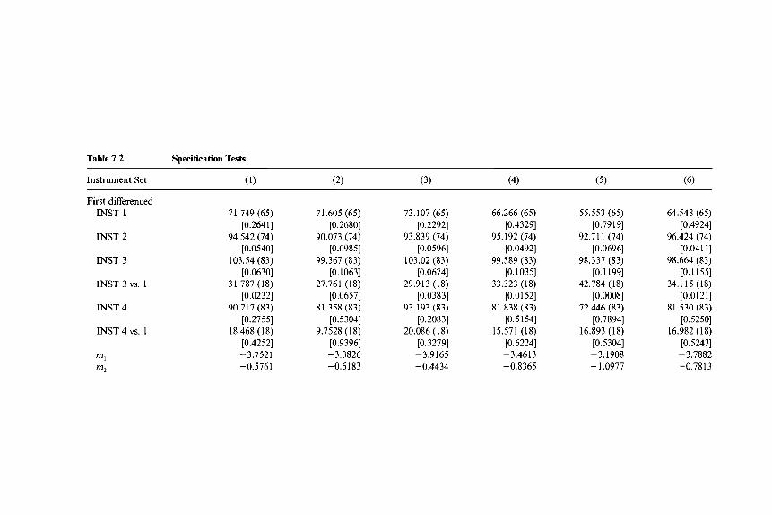
Table 7.2 Specification Tests

Instrument Set (1) (2) (3) (4) (5) (6)

First differenced INST 1 71.749 (65) 71.605 (65) 73.107 (65) 66.266 (65) 55.553 (65) 64.548 (65)

[0.2641] [0.2680] [0.2292] [0.4329] [0.7919] [0.4924] INST 2 94.542 (74) 90.073 (74) 93.839 (74) 95.192 (74) 92.711 (74) 96.424 (74)

[0.0540] [0.0985] [0.0596] [0.0492] [0.0696] [0.0411] INST 3 103.54 (83) 99.367 (83) 103.02 (83) 99.589 (83) 98.337 (83) 98.664 (83)

[0.0630] [O. 10631 [0.0674] [O. 10351 [0.1199] [0.1155] INST 3 vs. 1 31.787 (18) 27.761 (18) 29.913 (18) 33.323 (18) 42.784 (18) 34.115 (18)

INST 4 90.217 (83) 81.358 (83) 93.193 (83) 81.838 (83) 72.446 (83) 81.530 (83) [0.2755] [0.5304] [0.2083] [0 .5 1 541 [0.7894] [0.5250]

INST 4 vs. 1 18.468 (18) 9.7528 (18) 20.086 (18) 15.571 (18) 16.893 (18) 16.982 (18) [0.4252] [0.9396] [0.3279] [0.6224] [O. 53041 [0.5243]

m1 -3.7521 -3.3826 -3.9165 -3.4613 -3.1908 -3.7882 m2 -0.5761 -0.6183 -0.4434 -0.8365 - 1.0971 -0.7813

[0.0232] [0.0657] [0.0383] [0.0152] [0.0008] [0.0121]

System (first differenced + level)

INST 5 96.612 (98) 91.246 (98) 104.77 (98) 92.476 (98) 82.899 (98) 90.580 (98) [0.5206] [0.6722] [0.3014] [0.6384] tO.86241 [0.6900]

INST 5 vs. 4 6.3958 (15) 9.8874 (15) 11.576 (15) 10.638 (15) 10.453 (15) 9.0498 (15) [0.9723] [0.8267] [0.7108] [0.7778] [0.7903] [0.8749]

Note: INST 1 to INST 4 refer to different instrument sets for the first-differenced equations. b,, y,, . . . , yf-J is common to all sets. The four sets differ by including explanatory variables of different periods as summarized in the following:

INST 1 Wage, income, infrastructure INST 2

INST 3 Wage, income, infrastructure Wage, income INST 4 Wage, income, infrastructure Labor quality, infrastructure

Wage, income, labor quality, infrastructure

INST 5 includes INST 4 for the first-differenced equations, plus (Ay,- , , Axt, Ax,+,) for the level equations, where Ax, = (labor quality, infrastructure) and

Rows labeled “INST 1” to “INST 5” report Sargan overidentification tests corresponding to moment conditions implied by the relevant instrument sets.

The three rows labeled “INST a vs. b” report Sargan-difference tests for comparing two sets of moment conditions implied by INST a and INST b. The statistics m, and m, test the first-differenced residuals for zero first-order and second-order autocorrelation, respectively. Both statistics are asymptoti-

Ax,- , = (wage, income, SEZ, ZONES).

Each cell contains the value of the test statistic, the degrees of freedom (parentheses) of the x2 distribution, and thep-value (brackets) of the test.

cally N(0,l) under the null.


The Arellano-Bond m, and m2 serial correlation statistics from the INST 4 case are also reported in table 7.2. The significant m, and insignificant mz statistics indicate that there is no serial correlation in the level residuals, justifying the use of y lagged two periods or more as instruments for the first-differenced equations and lagged Ay for the level equations; that is, the moment conditions (C2) and (C5) in appendix C are valid. The system GMM estimates reported in table 7.1 are obtained by using the enlarged instrument set INST 5, which contains INST 4 for the first- differenced equations, plus (AY,-~, Ax,, Axr- ,) for the level equations, where Ax, = (labor quality, infrastructure) and Ax,-, = (wage, income, SEZ, ZONES). As can be seen from the last two rows of table 7.2, neither the overidentification test nor the Sargan-difference test rejects the additional level moment conditions, and this justifies the extra assumptions needed for the more efficient system GMM approach.

Table 7.1 shows that all the explanatory variables except university education have the expected sign. The coefficient for the lagged dependent variable is highly significant and quite stable. It is on average about 0.5, indicating a strong but not overwhelming self-reinforcing effect of the dependent variable’s past value on its current value. The coefficient for real wage is also quite significant and stable, ranging from -0.35 to -0.68, indicating that a 1 percent increase in a region’s wage costs would tend to re- duce its FDI by about half a percent. The coefficient of per capita income is significant and lies in the vicinity of 0.7 across different specifications.

Using the density of all roads as a proxy for infrastructure, columns (l), (2), and ( 3 ) of table 7.1 report estimation results for three alternative indicators of labor quality. The first two are university education and secondary education, and the third is the ratio of farming to nonfarming population, which is negatively correlated with the educational level of the population. None of the coefficients for these labor quality indicators is statistically significant, and university education is even of the wrong sign. We shall come back later to the role of labor quality as a determinant of FDI in China in section 7.5.

To consider other combinations of the proxies, we use secondary school for labor quality and the density of high-grade paved roads and that of railways for infrastructure. The coefficient estimates for these two infrastructure variables (cols. [4] and [5], respectively) were both insignificant, and even with the wrong sign in the case of railways. One explanation for the last result is that railways were mostly built in the past to support a planned economy and are not a very good indicator of the infrastructure that is needed to attract FDI.

The results for the combination of university education and high-grade paved roads are given in column (6). The coefficient for university education is still negative but getting smaller in magnitude as well as statistical significance.


The coefficient for the density of all roads is between 0.2 and 0.3, indicating that a 1 percent increase in a region’s roads would increase its FDI by 0.2 to 0.3 percent. The policy variable SEZ is statistically significant in all cases, and the policy variable equal to the sum of the other three zones (ZONES) is significant in all cases but two (cols. [l] and [3] ) . A comparison of the magnitude of the coefficients for SEZ and ZONES suggests that a Special Economic Zone was on average as effective as three to eleven other zones. Such a difference in the relative magnitude of their impact on FDI is consistent with the fact that Special Economic Zones gave much more favorable treatment to FDI than did the other policy designations.

7.5 Comparison with Other Studies

As in Cheng and Kwan (1999b), we have found a strong positive self- reinforcing effect of FDI on itself, which is consistent with the agglomeration effect identified by Head and Ries (1996). In addition, both regional income and good infrastructure (roads) contributed to FDI, although high-grade paved roads did not perform any better than all roads. In contrast with Chen’s (1996) finding that wages did not affect FDI and Head and Ries’s (1996) finding that the effect of wages was negligible, wage cost had a negative effect on FDI.

As expected, the coefficients for SEZ and ZONES are both significantly positive. The evidence reaffirms the well-known fact that the Special Eco- nomic Zones, which are close to Hong Kong and Taiwan, were more successful than the other zones in attracting FDI to China.

None of the education variables serving as proxies for labor quality had a significant impact on FDI, as first found by Cheng and Zhao (1995) and later in Cheng and Kwan (1999b). Together with our earlier work, a total of six proxies for labor quality have failed to show any significantly positive effect on FDI stock, indicating that the negative finding might not be explained away by the poor choice of any particular proxy. However, FDI from Japan and the United States tended to be concentrated in major cities known for their labor quality (namely, Beijing, Shanghai, and Tian- jin).’ Thus, even though labor quality is not a significant determinant of the total FDI received by each of the regions, it might be significant for FDI originating from the developed economies.

A related explanation is that much of the FDI was in labor-intensive manufacturing industries and in real estate. Labor quality is not particularly crucial in these industries, suggesting that lumping FDI in different industries may have the effect of confounding their differential under- lying determinants.

9. See Cheng (1994, table 15). FDI from Hong Kong and Taiwan tended to concentrate in the coastal regions, in particular, Guangdong, Fujian, Zhejiang, and Jiangsu.


7.6 Actual and Equilibrium Stocks of Foreign Direct Investment

Using the estimated equation, we can recover the unobserved equilibrium stock of FDI, y,T, and compare it with the actual (i.e., realized) stock of FDI, y,. The equilibrium stock is interesting not only because it mea- sures a region’s potential for absorbing FDI but also because its movement reflects the comparative static effect of changes in policy and other exogenous variables without the interference of the self-reinforcing effect and adjustment cost effect.

To highlight the difference between the equilibrium and realized stocks, we focus on the series of medians and quartiles computed from the regional distributions over the years. Figure 7.2 reports the paths of the actual and equilibrium median stock growth rates, whereas figure 7.3 high- lights the regional distributions of the deviation of actual FDI stock from equilibrium, where the equilibrium entities are calculated using the coefficients reported in column (2) of table 7.1.’O The equilibrium stock growth rates reveal the impacts of a few well-known events. The big dip in 1986 was due to a deterioration in the overall investment environment that prompted the government to introduce the “Twenty-Two Articles” in October of that year in order to stimulate FDI. The Tiananmen event in 1989 had a strong negative impact on the equilibrium growth rate, but the impact on the realized growth rate was hardly discernible. Deng Xiao- ping’s tour of south China in spring 1992 helped push the country’s open door policy back on track, resulting in a significant increase in the equilibrium growth rate. To cool the national economy and to discourage FDI in real estate, macroeconomic controls in 1994 brought down both the equilibrium and actual growth rates of FDI stock.

We calculate the deviation of the realized stock from the equilibrium stock to obtain a region’s potential for absorbing further FDI. This is the potential FDI that can be achieved under the assumption that the equilibrium stock stays at the existing level forever. Figure 7.3 summarizes the panel data of such deviations from equilibrium by the paths of the median and the lower and upper quartiles. As can be seen, over the years, the realized stock tends to converge to the equilibrium, but the convergence is occasionally disturbed by major policy shifts such as the Twenty- Two Articles and Deng’s south China tour, mentioned above. Interestingly, there is also a tendency toward convergence among the regions, as indi- cated by the shrinking dispersions over the years. Notice that the convergence is not in the stock of FDI a region will eventually achieve; rather, the convergence is in terms of the deviation of a region’s actual FDI stock from its equilibrium stock, which has little tendency to converge. That is

10. Using the coefficients given in col. (1) of table 7.1 would not make much difference in the equilibrium stocks and growth rates.


1 .o

0.8 - r

0.6

s 0.4

0.2

0.0

c - E -

-0.2 4 I 1984 1985 1988 1987 1988 1989 1990 1991 1992 1993 1994 1995

year

Fig. 7.2 Median annual growth of FDI stock

0.0 ,

-0.2

-0.4

-0.6

-0.8

-1.4 J 1983 1984 1985 1906 1987 1988 1989 1990 1991 1992 1993 1994 1995

Fig. 7.3 Deviation of actual FDI stock from equilibrium

to say, there is only convergence in the ratio of actual to potential FDI stocks but not convergence in the FDI stocks themselves.

The time-specific effects are depicted in figure 7.4, which clearly shows the effects of the 4 June event in 1989, Deng’s tour in 1992, and the macroeconomic controls in 1994 and 1995. The region-specific effects are depicted in figure 7.5, where the regions are ordered by distance from Hong


0.6

0.5

0.4

0.3

0.2

0.1

0.0 la Fig. 7.4 Time-specific effects (annual increment)

Fig. 7.5 Region-specific effects

Kong. As can be seen, the three regions closest to Hong Kong, namely, Guangdong, Guangxi, and Hainan, exhibit very strong positive effects. But proximity to Hong Kong does not explain everything, because Shang- hai, Tianjin, Beijing, and even Xinjiang also had strong region-specific factors that attracted FDI. Moreover, Guangdong, Hainan, and Fujian not only are close to Hong Kong and Taiwan but also possess Special Economic Zones. In the case of Shanghai, Tianjin, and Beijing, they were


China’s three most advanced cities. In addition, Shanghai began to have its own version of the Special Economic Zone (the Pudong New Zone) in 1990. These findings are consistent with the general observation that the determinants of export-oriented FDI are quite different from those of domestic-market-oriented FDI.

7.7 Concluding Remarks

With minor quantitative variations, our findings are very similar to those obtained in Cheng and Kwan (1999b). They not only are broadly consistent with the comparative statics results obtained in the literature on the location of FDI in the United States, China, and other countries but also provide support to existing studies that have empirically identified the self-reinforcing effect of FDI.

By integrating the traditional comparative statics theory of FDI location choice into a model of natural growth, our model has provided a better vantage point for understanding the potential determinants of FDI. The size of a region’s market as approximated by regional income has a positive effect, but wage cost has a negative effect on FDI. Good infrastructure as measured by the density of all roads attracts FDI, but the effect of the labor quality variables is insignificant. In fact, the coefficient for university education had the wrong sign. The positive impact of Spe- cial Economic Zones is far greater than that of the other key policy designations, including Open Coastal Cities, Economic and Technological De- velopment Zones, and Open Coastal Areas. There was no convergence in the equilibrium FDI stocks of the regions between 1985 and 1995; there was, however, convergence in the deviation of actual from equilibrium FDI.

Despite the use of six different proxies, we have not found any significantly positive effect of labor quality on FDI in China. Nevertheless, regions with high-quality labor (i.e., the centrally administered municipalities) were indeed successful in attracting FDI from Japan and the United States. Together these two facts suggest that it would be interesting for future research to analyze the determinants of FDI by source economy.


Appendix A

Table 7A.1 Definition of Variables

1. FDI stock 2. University education

3. Secondary education

4. Fardnonfarm

5. All roads 6. High-grade paved roads 7. Railway 8. Wage 9. Per capita income

10. SEZ

11. ZONES

Cumulative per capita real FDI at the end of year t Number of teachers and staff in institutions of higher edu-

cation (universities, colleges, and graduate schools) per 10,000 population

Number of teachers and staff in secondary schools (special- ized and regular) per 10,000 population

Ratio of population employed in the farming sector to nonfarming sector

Roads (kdkm2 of land mass) High-grade paved roads (km/km2 of land mass) Railway (km/kmz of land mass) Real wage Per capita real regional income Number of Special Economic Zones + 1, where 1 is added

to allow for zero SEZ in many regions 1 + Sum of numbers of Open Coastal Cities, Economic and

Technological Development Zones, and Open Coastal Areas

Appendix B Additional Explanations

The FDI data were obtained from China’s Ministry of Foreign Trade and Economic Cooperation, and most of the other data are from various issues of China Statistical Yearbook.

Price DeJutors. The deflator for FDI is the U.S. producer price index of capital equipment published by the U.S. Bureau of Labor Statistics. The deflator for per capita real income is the consumer price index of each region.

Regional Income (RI) . Regional income data are only available up to 1992; figures for 1993-95 are interpolated from the corresponding regional GDP data that replace the national income data starting from 1993. We first estimate a fixed-effects model, InRI,, = a, + p lnGDP, + E,,, using data for the interim period 1990-92 during which both RI and GDP are available. RI figures for 1993-95 are then interpolated from the estimated equation using the available GDP data.


Appendix C

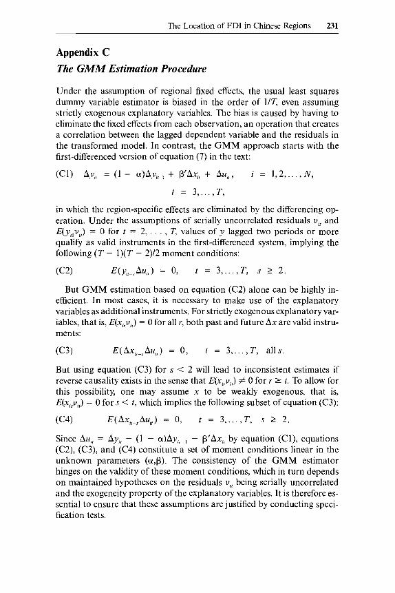
The GMM Estimation Procedure

Under the assumption of regional fixed effects, the usual least squares dummy variable estimator is biased in the order of 1/T, even assuming strictly exogenous explanatory variables. The bias is caused by having to eliminate the fixed effects from each observation, an operation that creates a correlation between the lagged dependent variable and the residuals in the transformed model. In contrast, the GMM approach starts with the first-differenced version of equation (7) in the text:

(Cl) Ay,, = (1 - C X ) A ~ , , - ~ + AX,, + Au,,, i = 1,2 ,..., N ,

t = 3, ..., T,

in which the region-specific effects are eliminated by the differencing operation. Under the assumptions of serially uncorrelated residuals uLt and E(y,,u,,) = 0 for t = 2, . . . , T, values of y lagged two periods or more qualify as valid instruments in the first-differenced system, implying the following (T - 1)(T - 2)/2 moment conditions:

(C2) E ( y , , _ 3 A ~ L , ) = 0, t = 3 ,..., T, s 2 2.

But GMM estimation based on equation (C2) alone can be highly in- efficient. In most cases, it is necessary to make use of the explanatory variables as additional instruments. For strictly exogenous explanatory variables, that is, E(x,,u,,) = 0 for all r, both past and future Ax are valid instruments:

(C3) E ( A X , _ ~ A U , ~ ) = 0, t = 3 ,... , T , alls.

But using equation (C3) for s < 2 will lead to inconsistent estimates if reverse causality exists in the sense that E(x,,u,,) # 0 for r 2 t. To allow for this possibility, one may assume x to be weakly exogenous, that is, E(xlsuZr) = 0 for s < t , which implies the following subset of equation (C3):

(C4) E ( A X ~ [ - ~ A U , , ) = 0, t = 3 ,..., T, s 2 2.

Since Au,, = Ayl, - (1 - a)Ay+, - AX,^ by equation (Cl), equations (C2), (C3), and (C4) constitute a set of moment conditions linear in the unknown parameters (a$). The consistency of the GMM estimator hinges on the validity of these moment conditions, which in turn depends on maintained hypotheses on the residuals ul, being serially uncorrelated and the exogeneity property of the explanatory variables. It is therefore es- sential to ensure that these assumptions are justified by conducting specification tests.


For the overidentified case in which the number of moment conditions q exceeds the number of unknown parameters k, the minimized GMM criterion function provides a specification test for the overall validity of the moment conditions (i.e., the Sargan test). The null hypothesis of no misspecification (i.e., all moment conditions valid) is rejected if the GMM criterion function registers a large value compared with a x2 distribution with q - k degrees of freedom. Another useful diagnostic is the Sargan- difference specification test that evaluates the validity of extra moment conditions in a nested case. For example, strict exogeneity implies extra moment conditions over that of weak exogeneity (i.e., condition [C4] is nested in [C3]). Let the minimized GMM criterion function for the nested, weak exogeneity case be s1 and that of the strict exogeneity case be s2, with the numbers of moment conditions for the two cases being q, and q2, respectively. By construction, q, > q, and s, > s,. The null hypothesis of strict exogeneity can be tested against the alternative of weak exogeneity by testing the validity of the extra moment conditions, using the Sargan- difference statistic s2 - s, compared with a x2 distribution of degrees of freedom q2 - 4,.

We also report a residual-based specification test suggested by Arellano and Bond (1991). Based on the differenced residuals, the Arellano-Bond m, and m2 serial correlation statistics, both distributed as N(0,l) in large sample, test the null hypotheses of zero first-order and second-order autocorrelation, respectively. An insignificant m, and/or significant m2 will issue warnings against the likely presence of invalid moment conditions due to serial correlation in the level residuals.

The GMM approach discussed so far utilizes moment conditions (C2), (C3), and (C4) based on the first-differenced equation (Cl). The first- differencing operation not only eliminates unobserved region-specific effects but also time-invariant explanatory variables for which only cross- sectional information is available. This is problematic in our application because the two policy variables of interest, SEZ (the number of Special Economic Zones in a region) and ZONES (the total number of Open Coastal Cities, Economic and Technological Development Zones, and Open Coastal Areas), are nearly time invariant so that their first differences are relatively uninformative, rendering the associated parameters close to being unidentified in the first-differenced system. Moreover, as demonstrated by Ahn and Schmidt (1995, 1997) and Blundell and Bond (1998), under a random-effects model, the first-differenced GMM estimator can suffer from serious efficiency loss, for potentially informative moment conditions are ignored in the first-difference approach. Following

11. See Arellano and Bond (1991) for the relevant formulas and proofs of the statistical distribution theory for various specification tests.


Blundell and Bond (1 998), we augment the first-differenced moment conditions (C2), (C3), and (C4) by the level moment conditions

(C5) E(uz,Aylr_l) = 0, t = 3 , . . . , T ,

which amounts to using lagged differences of y as instruments in the level equation (7). For strictly exogenous explanatory variables, there are level moment conditions

(C6) E(u,,Axi,-, j = 0, t = 2 , . . . , T , all s;

and for weakly exogenous explanatory variables, the appropriate level moment conditions would be

(C7) E(u,rAxll+s) = 0 , t = 3,. . . , T , s 2 1.

The Blundell-Bond system GMM estimator is obtained by imposing the enlarged set of moment conditions (C2) through (C7). By exploiting more moment conditions, the system GMM estimator has a smaller as- ymptotic variance (more efficient) than the first-differenced GMM estimator that uses only the subset (C2), (C3), and (C4). The validity of the level moment conditions (C5), (C6), and (C7) depends on a standard random- effects specification of equation (7) in which

(C8) E ( q ) = E(u,,) = E ( u t r q ) = 0,

E(vL,v,j = 0,

E(y~ ,u l r ) = 0,

for i = 1 , . . . , N a n d t = 2 ,... ,T ,

for i = 1 , . . . , N a n d t # s,

for i = 1,. . . , Nand t = 2, . . . , T ,

plus two additional assumptions: (a) E(ut3Ayt2) = 0, a restriction on the initial value process generating y, , , and (b) E(q,Ax,J = 0, which requires that the region-specific effects be uncorrelated with the explanatory variables in first difference.

The efficiency gain from imposing the level moment conditions certainly does not come free; we do make more assumptions the violation of which may lead to bias. Since the first-differenced moment conditions are nested within the augmented set, the additional level moment conditions can be tested by the Sargan-difference testing procedure described above, using the GMM criterion functions from the first-difference and the system approaches. In addition, invalid level moment conditions can also be de- tected by the Sargan overidentification test from the system GMM estimation.


References

Ahn, S. C., and P. Schmidt. 1995. Efficient estimation of models for dynamic panel data. Journal of Econometrics 68:5-27.

. 1997. Efficient estimation of dynamic panel data models: Alternative assumptions and simplified estimation. Journal of Econometrics 76:309-21.

Anderson, T. W., and C. Hsiao. 1981. Estimation of dynamic models with error components Journal of the American Statistical Association 76:598-606.

. 1982. Formulation and estimation of dynamic models using panel data. Journal of Econometrics 18:47-82.

Arellano, M., and S. Bond. 1991. Some tests of specification for panel data: Monte Carlo evidence and an application to employment equation. Review of Economic Studies 58:277-97.

Arellano, M., and 0. Bover. 1995. Another look at the instrumental variable estimation of error-components models. Journal of Econometrics 68:29-5 1.

Blundell, R., and S. Bond. 1998. Initial conditions and moment restrictions in dynamic panel data models. Journal of Econometrics 87: 1 15-43.

Chen, C. 1996. Regional determinants of foreign direct investment in mainland China. Journal of Economic Studies 23: 18-30.

Cheng, L. K. 1994. Foreign direct investment in China. OECD Report no. COMI DAFFElIMElTD (94) 129. Paris: Organization for Economic Cooperation De- velopment, November.

Cheng, L. K., and Y. Kwan. 1999a. FDI stock and its determinants. In Foreign direct investment and economic growth in China, ed. Y. Wu, 42-56. Cheltenham, England: Elgar.

. 1999b. What are the determinants of the location of foreign direct investment? The Chinese experience. Journal of International Economics. Forth- coming.

Cheng, L. K., and H. Zhao. 1995. Geographical patterns of foreign direct investment in China: Location, factor endowments, and policy incentives. Hong Kong: Hong Kong University of Science and Technology, Department of Eco- nomics, February. Mimeograph.

Chow, G. C. 1967. Technological change and the demand for computers. American Economic Review 57:1117-30.

Coughlin, C., J. V. Terza, and V. Arromdee. 1991. State characteristics and the location of foreign direct investment within the United States. Review of Eco- nomics and Statistics 73:675-83.

Friedman, J., H. Fung, D. Gerlowski, and J. Silberman. 1996. A note on “State characteristics and the location of foreign direct investment within the United States.” Review of Economics and Statistics 78:367-68.

Friedman, J., D. Gerlowski, and J. Silberman. 1992. What attracts foreign multinational corporations? Evidence from branch plant location in the United States. Journal of Regional Science 32:403-18.

Head, K., and J. Ries. 1996. Inter-city competition for foreign investment: Static and dynamic effects of China’s incentive areas. Journal of Urban Economics 40:38-60.

Head, K., J. Ries, and D. Swenson. 1995. Agglomeration benefits and location choice: Evidence from Japanese manufacturing investment in the United States. Journal of International Economics 38:223-47.

Hill, S., and M. Munday. 1995. Foreign manufacturing investment in France and the U.K.: A regional analysis of locational determinants Tudschrgt voor Eco- nomische en Sociale Geograje 86:311-27.


Hines, J. 1996. Altered states: Taxes and the location of foreign direct investment

Holtz-Eakin, D., W. Newey, and H. Rosen. 1988. Estimating vector autoregres-

Hsiao, C. 1986. Analysis of panel data. Cambridge: Cambridge University Press. 0 Huallachain, B., and N. Reid. 1997. Acquisition versus greenfield investment:

The location and growth of Japanese manufacturers in the United States. Re- gional Studies 3 1 :403-16.

Organization for Economic Cooperation and Development (OECD). 1992. The OECD declaration and decisions on international investment and multinational enterprises: 199 1 review. Paris: Organization for Economic Cooperation and Development.

Rozelle, S., Y Ying, and M. Barlow. N.d. Targeting transaction costs: An evalua- tion of investment incentive policies in China’s foreign trade zones. Stanford, Calif.: Stanford University, Food Research Institute, Mimeograph.

Sevestre, P., and A. Trognon. 1996. Dynamic linear models. In The econometrics of panel data: Handbook of theory and applications, 2d rev. ed., ed. L. Matyas and P. Sevestre, 120-44. Dordrecht: Kluwer.

Smith, D., and R. Florida. 1994. Agglomeration and industrial location: An econometric analysis of Japanese affiliated manufacturing establishments in automotive-related industries. Journal of Urban Economics 36:23-41.

Wheeler, D., and A. Mody. 1992. International investment location decisions: The case of US. firms. Journal of International Economics 33:57-76.

Woodward, D. 1992. Locational determinants of Japanese manufacturing startups in the United States. Southern Economic Journal 58:690-708.

in America. American Economic Review 86: 1076-94.

sions with panel data. Econometrica 56:1371-95.

Comment Yumiko Okamoto

I much appreciated the paper by Cheng and Kwan. In fact, I analyzed the capacity of noncoastal areas of China to utilize FDI as part of their development strategies last year. Since whether FDI could be part of a region’s development strategy depends largely on the determinants of FDI location, this paper is clearly relevant to my research.

Cheng and Kwan examine the determinants of the location of FDI in China by combining the comparative statics theory of FDI location and Chow’s partial adjustment model. The combination of the two is an inno- vative part of their paper. They find that the magnitude of national and regional markets, good infrastructure, and the number of Special Economic Zones have positive effects on FDI, while wage cost has a negative effect. Surprisingly, the education variable has no significant effect on FDI. They also find strong evidence for an agglomeration effect.

The separation of relative from absolute convergence among the regions in absorbing FDI is particularly interesting. In my study I also found that although there is no evidence whatsoever of convergence in the absolute

Yumiko Okamoto is associate professor of economics at Nagoya University.


amount of FDI inflow between coastal areas and inland China, inland China has also begun attracting FDI in the past couple of years. This phenomenon seems to be confirmed by Cheng and Kwan’s regression results. If so, there is still room for inland China to attract more FDI by adopting appropriate policies regardless of whether there is convergence among regions in absorbing FDI in absolute terms.

About investigating the determinants of FDI location, I have one suggestion. It might be interesting to repeat the analysis separating FDI from Hong Kong and Taiwan and FDI from other industrialized countries such as the United States and Japan. I found the regional investment pattern between the two to be different. Also several past studies have seemed to suggest that the investment behavior of overseas Chinese differs from that of others. Therefore, the explicit introduction of FDI source into the research might enrich the study further.

I also found the inclusion of a variable to represent nationwide as well as regional markets interesting. This seemed to control for a demand factor that might influence the whole region simultaneously. If that is the case, it might also be interesting to introduce a variable that represents a regionwide supply-side factor for FDI as well.

Finally, the fact that no education variable shows any statistical significance as a determinant of FDI location bothers me. I wonder whether this is due to a statistical problem such as multicollinearity or, on the other hand, whether it suggests that investors do not care about the quality of the labor force in the case of China.

Comment Shang-Jin Wei

This well-written paper investigates an important topic. A number of studies have looked into the consequences of FDI in China (e.g., Lardy 1992), including some that used Chinese city-level data (e.g., Wei 1995, 1996). This paper, following other papers that these authors have done (Cheng and Zhao 1995; Cheng and Kwan 1999), is among the first that studies the determinants of FDI locations within China.

The paper very sensibly applies a partial adjustment framework to the specification, and very properly uses a GMM method for estimation and specification tests. The version of the paper presented here also represents significant improvement over the first draft presented at the conference.

Shang-Jin Wei is associate professor of public policy at the Kennedy School of Govern- ment, Harvard University, and a faculty research fellow of the National Bureau of Economic Research. During 1999-2000, he serves as an advisor on anticorruption issues at the World Bank.


So I will confine my revised comments to a few points that I would bring to the reader’s attention.

Interpretation of a Positive Coefficient on the Past FDI Stock

The main equation estimated in the paper is what is called a partial adjustment specification: the change in the log (FDI stock) is regressed on the difference between lagged log (FDI stock) and an equilibrium level of FDI stock, which is a function a vector of “state” variables. Several papers in the literature (including the earlier version of this paper) applied a framework like this and interpreted a positive coefficient on the lagged FDI stock as evidence of agglomeration. Agglomeration (which is moti- vated by some kind of externality) and partial adjustment (which is moti- vated by convex adjustment costs) are conceptually very different. But both can produce a positive coefficient on the lagged FDI stock. I am pleased to see that the revised paper takes into account my suggestion that the specification in the paper cannot disentangle the agglomeration effect versus partial adjustment. I would suggest that the authors make this point more clearly and forcefully, as it could help to correct a common impression one gets from several papers in the literature that adopt this interpretation.

Possible Missing Fixed Effects?

In an effort to estimate certain virtually time-invariant policy fixed effects (i,e., numbers of Special Economic Zones, Open Coastal Cities, etc.), the authors add what they call level moment conditions. This ability to estimate the policy fixed effects comes with a possible cost; namely, it may have reintroduced missing fixed effects that the first-difference is supposed to eliminate. Specifically, distance and linguistic connection between the source countries and host regions (countries) were found to be important determinants of bilateral FDI in the literature (see, e.g., Wei 1996, 1997) but are not included in the current paper. For example, the facts that Guangdong is the only province that shares a common dialect with Hong Kong and that it is closest in distance to Hong Kong, the biggest source of FDI into China, is most likely correlated with the fact that it is the biggest recipient of FDI among all provinces. That coastal provinces/ municipalities have the largest number of English- (or Japanese-)speak- ing personnel is also likely correlated with the observation that there is substantially more FDI in coastal areas than inland.

Interpretation of the Policy Effect

The authors use two variables to capture what they term the policy effects: SEZ, the number of Special Economic Zones in a region; and ZONES, the total number of Open Coastal Cities, Economic and Techno- logical Development Zones, and Open Coastal Areas. These variables are


virtually time-invariant. They found that both variables produce positive coefficients, and the coefficient for SEZ is at least three times as large as the one on ZONES. They interpret this as the effect of special favorable treatment in these zones that were offered to foreign firms.

It is quite likely that the special policies do alter the locational choice of the foreign firms. However, the positive coefficients reported may very well also reflect the effects of other missing variables rather than exclu- sively the effects of either SEZs or other zones. This is, of course, related to the previous point. Specifically, three of the four initial Special Eco- nomic Zones are located in Guangdong Province alone (the other is in Fujian province, the closest province to Taiwan). Guangdong attracts more FDI than the model predicts, for whatever reason (some were specu- lated in the previous observation), so the SEZ dummy may simply capture this Guangdong effect, regardless of the true effect of the policies within the Special Economic Zones. Likewise, the so-called Open Coastal Cities or Open Coastal Areas are near the coast. Therefore, the positive coefficient on the ZONES variable could be just a relabeling of the fact that the coastal provinces receive more FDI on average.

Overall, reading this paper is a rewarding experience. None of the above comments should detract from the fact that this is a nice piece of work both for understanding locational decisions of multinational firms in general and for understanding FDI into China in particular.

References

Cheng, Leonard K., and Yum K. Kwan. 1999. FDI stock and its determinants. In Foreign direct investment and economic growth in China, ed. Y Wu, 42-56. Cheltenham, England: Edward Elgar.

Cheng, Leonard K., and Haiying Zhao. 1995. Geographic patterns of foreign direct investment in China: Location, factor endowment, and policy incentives. Hong Kong University of Science and Technology, Department of Economics, February. Unpublished paper.

Lardy, Nicholas. 1992. Foreign trade and economic reform in China, 1978-1990. Cambridge: Cambridge University Press.

Wei, Shang-Jin. 1995. The open door policy and China’s rapid growth: Evidence from city-level data. In Growth theories in light of the East Asian experience, ed. T. Ito and A. 0. Krueger. Chicago: University of Chicago Press.

. 1996. Foreign direct investment in China: Sources and consequences. In Financialderegulation and integration in East Asia, ed. T. Ito and A. 0. Krueger. Chicago: University of Chicago Press.

. 1997. How taxing is corruption on international investors? NBER Work- ing Paper no. 6030. Cambridge, Mass.: National Bureau of Economic Research. (Forthcoming, Review of Economics and Statistics)

The Location of Foreign Direct Investment in Chinese … Location of Foreign Direct Investment in...

Documents

Transcript of The Location of Foreign Direct Investment in Chinese … Location of Foreign Direct Investment in...