The Limit Point of the Pentagram Map and Infinitesimal ...

Q. Aboud and A. Izosimov (2020) “The Limit Point of the Pentagram Map and Infinitesimal Monodromy,”International Mathematics Research Notices, Vol. 00, No. 0, pp. 1–15doi:10.1093/imrn/rnaa258

The Limit Point of the Pentagram Map and InfinitesimalMonodromy

Quinton Aboud and Anton Izosimov∗

Department of Mathematics, University of Arizona, 85721, USA

∗Correspondence to be sent to: e-mail: [email protected]

The pentagram map takes a planar polygon P to a polygon P′ whose vertices are the

intersection points of the consecutive shortest diagonals of P. The orbit of a convex

polygon under this map is a sequence of polygons that converges exponentially to a

point. Furthermore, as recently proved by Glick, coordinates of that limit point can be

computed as an eigenvector of a certain operator associated with the polygon. In the

present paper, we show that Glick’s operator can be interpreted as the infinitesimal

monodromy of the polygon. Namely, there exists a certain natural infinitesimal pertur-

bation of a polygon, which is again a polygon but in general not closed; what Glick’s

operator measures is the extent to which this perturbed polygon does not close up.

1 Introduction

The pentagram map, introduced by Schwartz [10], is a discrete dynamical system on the

space of planar polygons. The definition of this map is illustrated in Figure 1: the image

of the polygon P under the pentagram map is the polygon P′ whose vertices are the

intersection points of the consecutive shortest diagonals of P (i.e., diagonals connecting

2nd-nearest vertices).

The pentagram map has been an especially popular topic in the past decade,

mainly due to its connections with integrability [8, 12] and the theory of cluster algebras

[2–4]. Most works on the pentagram map regard it as a dynamical system on the space

Communicated by Prof. Igor KricheverReceived June 12, 2020; Revised June 12, 2020; Accepted August 19, 2020

© The Author(s) 2020. Published by Oxford University Press. All rights reserved. For permissions,

please e-mail: [email protected].

2 Q. Aboud and A. Izosimov

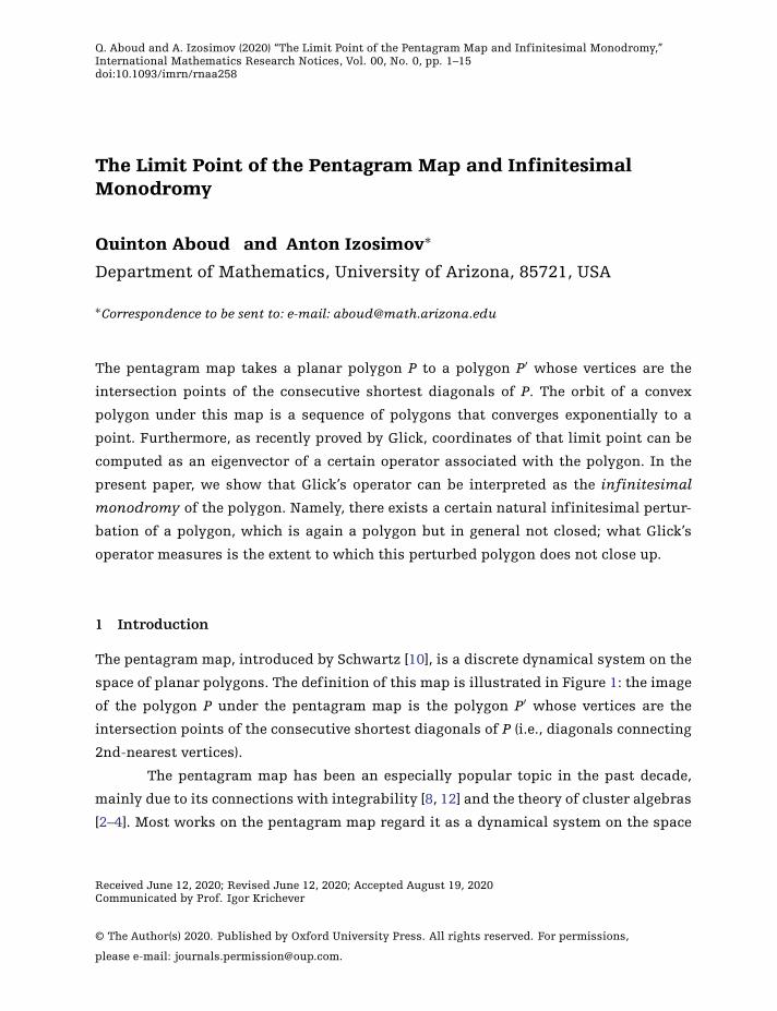
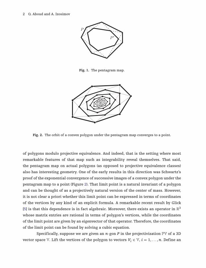
Fig. 1. The pentagram map.

Fig. 2. The orbit of a convex polygon under the pentagram map converges to a point.

of polygons modulo projective equivalence. And indeed, that is the setting where most

remarkable features of that map such as integrability reveal themselves. That said,

the pentagram map on actual polygons (as opposed to projective equivalence classes)

also has interesting geometry. One of the early results in this direction was Schwartz’s

proof of the exponential convergence of successive images of a convex polygon under the

pentagram map to a point (Figure 2). That limit point is a natural invariant of a polygon

and can be thought of as a projectively natural version of the center of mass. However,

it is not clear a priori whether this limit point can be expressed in terms of coordinates

of the vertices by any kind of an explicit formula. A remarkable recent result by Glick

[5] is that this dependence is in fact algebraic. Moreover, there exists an operator in R3

whose matrix entries are rational in terms of polygon’s vertices, while the coordinates

of the limit point are given by an eigenvector of that operator. Therefore, the coordinates

of the limit point can be found by solving a cubic equation.

Specifically, suppose we are given an n-gon P in the projectivization PV of a 3D

vector space V. Lift the vertices of the polygon to vectors Vi ∈ V, i = 1, . . . , n. Define an

Pentagram Map and Infinitesimal Monodromy 3

operator GP : V → V by the formula

Gp(V) := nV −n∑

i=1

Vi−1 ∧ V ∧ Vi+1

Vi−1 ∧ Vi ∧ Vi+1Vi, (1)

where all indices are understood modulo n. Note that this operator does not change

under a rescaling of Vis and hence depends only on the polygon P. What Glick proved

is that the limit point of successive images of P under the pentagram map is one of

the eigenvectors of GP (equivalently, a fixed point of the associated projective mapping

PV → PV).

We believe that the significance of Glick’s operator actually goes beyond the

limit point. In particular, as was observed by Glick himself, the operator GP has a

natural geometric meaning for both pentagons and hexagons. Namely, by Clebsch’s

theorem, every pentagon is projectively equivalent to its pentagram map image, and

it turns out that the corresponding projective transformation is given by GP − 3I, where

I is the identity matrix. Indeed, consider, for example, the 1st vertex of the pentagon

and its lift V1. Then, the above formula gives

(GP − 3I)(V1) = V1 − V2 ∧ V1 ∧ V4

V2 ∧ V3 ∧ V4V3 − V3 ∧ V1 ∧ V5

V3 ∧ V4 ∧ V5V4.

Taking the wedge product of this expression with V2 ∧ V4 or V3 ∧ V5, we get zero. This

means that

(GP − 3I)(V1) ∈ span(V2, V4) ∩ span(V3, V5),

so the corresponding point in the projective plane is the intersection of diagonals of the

pentagon. Furthermore, since Glick’s operator is invariant under cyclic permutations,

the same holds for all vertices, meaning that the operator GP−3I indeed takes a pentagon

to its pentagram map image.

Likewise, the 2nd iterate of the pentagram map on hexagons also leads to an

equivalent hexagon and the equivalence is again realized by GP − 3I. Finally, notice

that for quadrilaterals GP − 2I is a constant map onto the intersection of diagonals.

These observations make us believe that the operator GP is per se an important object

in projective geometry, whose full significance is yet to be understood.

In the present paper, we show that Glick’s operator GP can be interpreted as

infinitesimal monodromy. To define the latter, consider the space of twisted polygons,

which are polygons closed up to a projective transformation, known as the monodromy.


Any closed polygon can be viewed as a twisted one, with trivial monodromy. To define

the infinitesimal monodromy, we deform a closed polygon into a genuine twisted one.

To construct such a deformation, we use what is known as the scaling symmetry. The

scaling symmetry is a 1-parametric group of transformations of twisted polygons that

commutes with the pentagram map. That symmetry was instrumental for the proof of

complete integrability of the pentagram map [8].

Applying the scaling symmetry to a given closed polygon P, we get a family Pz of

polygons depending on a real parameter z and such that P1 = P. Thus, the monodromy

Mz of Pz is a projective transformation depending on z, which is the identity for

z = 1. By definition, the infinitesimal monodromy of P is the derivative dMz/dz at z = 1.

This makes the infinitesimal monodromy an element of the Lie algebra of the projective

group PGL(P2), that is, a linear operator on R3 defined up to adding a scalar matrix. The

following is our main result.

Theorem 1.1. The infinitesimal monodromy of a closed polygon P coincides with

Glick’s operator GP, up to the addition of a scalar matrix.

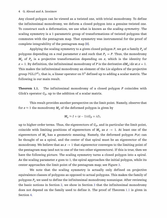
This result provides another perspective on the limit point. Namely, observe that

for z ≈ 1 the monodromy Mz of the deformed polygon is given by

Mz ≈ I + (z − 1)(GP + λI),

up to higher-order terms. Thus, the eigenvectors of GP, and in particular the limit point,

coincide with limiting positions of eigenvectors of Mz as z → 1. At least one of the

eigenvectors of Mz has a geometric meaning. Namely, the deformed polygon P(z) can

be thought of as a spiral, and the center of that spiral must be an eigenvector of the

monodromy. We believe that as z → 1 that eigenvector converges to the limiting point of

the pentagram map (and not to one of the two other eigenvectors). If this is true, then we

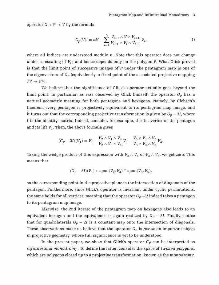
have the following picture. The scaling symmetry turns a closed polygon into a spiral.

As the scaling parameter z goes to 1, the spiral approaches the initial polygon, while its

center approaches the limit point of the pentagram map; see Figure 3.

We note that the scaling symmetry is actually only defined on projective

equivalence classes of polygons as opposed to actual polygons. This makes the family of

polygons Pz we used to define the infinitesimal monodromy nonunique. After reviewing

the basic notions in Section 2, we show in Section 3 that the infinitesimal monodromy

does not depend on the family used to define it. The proof of Theorem 1.1 is given in

Section 4.


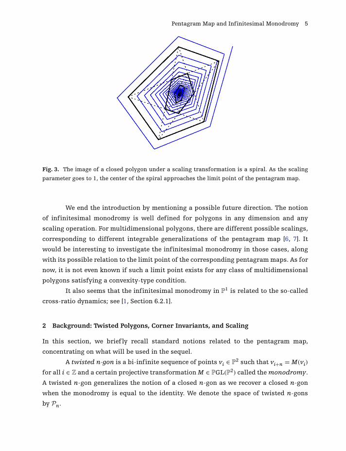
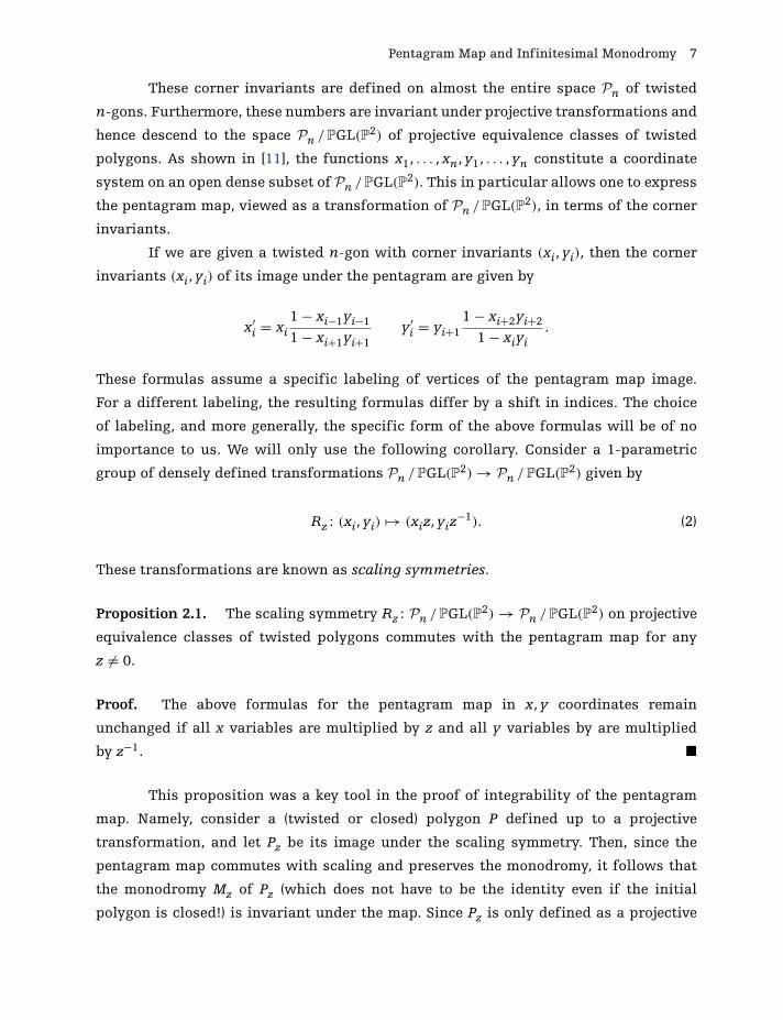
Fig. 3. The image of a closed polygon under a scaling transformation is a spiral. As the scaling

parameter goes to 1, the center of the spiral approaches the limit point of the pentagram map.

We end the introduction by mentioning a possible future direction. The notion

of infinitesimal monodromy is well defined for polygons in any dimension and any

scaling operation. For multidimensional polygons, there are different possible scalings,

corresponding to different integrable generalizations of the pentagram map [6, 7]. It

would be interesting to investigate the infinitesimal monodromy in those cases, along

with its possible relation to the limit point of the corresponding pentagram maps. As for

now, it is not even known if such a limit point exists for any class of multidimensional

polygons satisfying a convexity-type condition.

It also seems that the infinitesimal monodromy in P1 is related to the so-called

cross-ratio dynamics; see [1, Section 6.2.1].

2 Background: Twisted Polygons, Corner Invariants, and Scaling

In this section, we briefly recall standard notions related to the pentagram map,

concentrating on what will be used in the sequel.

A twisted n-gon is a bi-infinite sequence of points vi ∈ P2 such that vi+n = M(vi)

for all i ∈ Z and a certain projective transformation M ∈ PGL(P2) called the monodromy.

A twisted n-gon generalizes the notion of a closed n-gon as we recover a closed n-gon

when the monodromy is equal to the identity. We denote the space of twisted n-gons

by Pn.


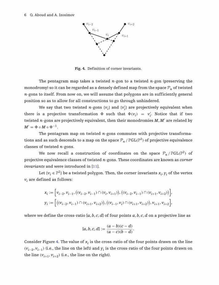
Fig. 4. Definition of corner invariants.

The pentagram map takes a twisted n-gon to a twisted n-gon (preserving the

monodromy) so it can be regarded as a densely defined map from the space Pn of twisted

n-gons to itself. From now on, we will assume that polygons are in sufficiently general

position so as to allow for all constructions to go through unhindered.

We say that two twisted n-gons {vi} and {v′i} are projectively equivalent when

there is a projective transformation � such that �(vi) = v′i. Notice that if two

twisted n-gons are projectively equivalent, then their monodromies M, M ′ are related by

M ′ = � ◦ M ◦ �−1.

The pentagram map on twisted n-gons commutes with projective transforma-

tions and as such descends to a map on the space Pn /PGL(P2) of projective equivalence

classes of twisted n-gons.

We now recall a construction of coordinates on the space Pn /PGL(P2) of

projective equivalence classes of twisted n-gons. These coordinates are known as corner

invariants and were introduced in [11].

Let {vi ∈ P2} be a twisted polygon. Then, the corner invariants xi, yi of the vertex

vi are defined as follows:

xi :=[vi−2, vi−1,

((vi−2, vi−1) ∩ (vi, vi+1)

),((vi−2, vi−1) ∩ (vi+1, vi+2)

)],

yi :=[(

(vi−2, vi−1) ∩ (vi+1, vi+2)),((vi−1, vi) ∩ (vi+1, vi+2)

), vi+1, vi+2

],

where we define the cross-ratio [a, b, c, d] of four points a, b, c, d on a projective line as

[a, b, c, d] := (a − b)(c − d)

(a − c)(b − d).

Consider Figure 4. The value of xi is the cross-ratio of the four points drawn on the line

(vi−2, vi−1) (i.e., the line on the left) and yi is the cross-ratio of the four points drawn on

the line (vi+1, vi+2) (i.e., the line on the right).


These corner invariants are defined on almost the entire space Pn of twisted

n-gons. Furthermore, these numbers are invariant under projective transformations and

hence descend to the space Pn /PGL(P2) of projective equivalence classes of twisted

polygons. As shown in [11], the functions x1, . . . , xn, y1, . . . , yn constitute a coordinate

system on an open dense subset of Pn /PGL(P2). This in particular allows one to express

the pentagram map, viewed as a transformation of Pn /PGL(P2), in terms of the corner

invariants.

If we are given a twisted n-gon with corner invariants (xi, yi), then the corner

invariants (xi, yi) of its image under the pentagram are given by

x′i = xi

1 − xi−1yi−1

1 − xi+1yi+1y′

i = yi+11 − xi+2yi+2

1 − xiyi.

These formulas assume a specific labeling of vertices of the pentagram map image.

For a different labeling, the resulting formulas differ by a shift in indices. The choice

of labeling, and more generally, the specific form of the above formulas will be of no

importance to us. We will only use the following corollary. Consider a 1-parametric

group of densely defined transformations Pn /PGL(P2) → Pn /PGL(P2) given by

Rz : (xi, yi) → (xiz, yiz−1). (2)

These transformations are known as scaling symmetries.

Proposition 2.1. The scaling symmetry Rz : Pn /PGL(P2) → Pn /PGL(P2) on projective

equivalence classes of twisted polygons commutes with the pentagram map for any

z �= 0.

Proof. The above formulas for the pentagram map in x, y coordinates remain

unchanged if all x variables are multiplied by z and all y variables by are multiplied

by z−1. �

This proposition was a key tool in the proof of integrability of the pentagram

map. Namely, consider a (twisted or closed) polygon P defined up to a projective

transformation, and let Pz be its image under the scaling symmetry. Then, since the

pentagram map commutes with scaling and preserves the monodromy, it follows that

the monodromy Mz of Pz (which does not have to be the identity even if the initial

polygon is closed!) is invariant under the map. Since Pz is only defined as a projective


equivalence class, this means that Mz is only defined up to conjugation. Nevertheless,

taking conjugation-invariant functions (e.g., appropriately normalized eigenvalues) of

Mz, we obtain, for every z, functions that are invariant under the pentagram map. It is

shown in [8] that the so-obtained functions commute under an appropriately defined

Poisson bracket and turn the pentagram map into a discrete completely integrable

system. See also [9] for a mode detailed proof. In our paper, we utilize pretty much the

same idea, but instead of looking at the eigenvalues of Mz, we will consider Mz itself. It

is not quite well defined, but we will show that its z derivative at z = 1 is and that it

coincides with Glick’s operator.

3 Infinitesimal Monodromy

In this section, we define the infinitesimal monodromy and show that it does not depend

on the choices we need to make to formulate the definition, namely on the way we lift the

scaling symmetry (2) from projective equivalence classes of polygons to actual polygons.

We start with a closed n-gon, P, in P2. Let [P] ∈ Pn /PGL(P2) be its projective

equivalence class. Then, applying the scaling transformation Rz given by (2) to [P], we get

a path Rz[P] in Pn /PGL(P2) such that R1[P] = [P]. Now, choose a smooth in z lift Pz of the

path Rz[P] to the space Pn of actual twisted polygons such that P1 = P (we will construct

an explicit example of such a lift later on). Denote by Mz ∈ PGL(P2) the monodromy of

Pz. It is a family of projective transformations such that M1 is the identity, M1 = I. This

family does depend on the choice of the lift Pz of the path Rz[P]. However, as we show

below, the tangent vector dMz/dz at z = 1 does not depend on that choice and this is

what we call the infinitesimal monodromy.

Definition 3.1. The infinitesimal monodromy of a closed polygon P is the derivative

dMz/dz at z = 1, where Mz is the monodromy of any path Pz of polygons such that P1 = 1

and [Pz] = Rz[P].

The infinitesimal monodromy is therefore a tangent vector to the projective

group PGL(P2) at the identity, and, upon a choice of basis, can be viewed as a 3 × 3

matrix defined up to addition of a scalar matrix. Our main result can thus be formulated

as follows.

Theorem 3.1 (=Theorem 1.1). The tangent vector to PGL(P2) represented by Glick’s

operator GP coincides with the infinitesimal monodromy of P.


The proof will be given in Section 4. But first, we need to check that

Definition 3.1 makes sense, that is, that the infinitesimal monodromy does not depend

on the choice of the path Pz. This is established by the following.

Proposition 3.2. Let Pz and P̃z be two families of polygons such that P1 = P̃1 is a closed

polygon and P̃z is projectively equivalent to Pz for every z. Then, for the monodromies

Mz and M̃z of these families, at z = 1, we have dMz/dz = dM̃z/dz.

Proof. Let �z be a projective transformation taking Pz to P̃z. Since P1 = P̃1, we

have that �1 = I (a generic n-gon in P2 does not admit any nontrivial projective

automorphisms, provided that n ≥ 4). Then, we know that the monodromies are related

by M̃z = �zMz�−1z . Differentiating this and using that �1 = I, we get

d

dz

∣∣∣∣ z=1M̃z = d

dz

∣∣∣∣ z=1Mz +[

d

dz

∣∣∣∣ z=1�z, M1

].

This identity in particular shows that the infinitesimal monodromy of a twisted polygon

is in general not well defined, due to the extra commutator term in the right-hand side.

But for a closed polygon, we have M1 = I, so the extra term vanishes and we get the

desired identity. �

Before we proceed to the proof of the main theorem, let us mention one property

of the infinitesimal monodromy.

Proposition 3.3. The infinitesimal monodromy of a closed polygon is preserved by the

pentagram map.

Proof. The pentagram map preserves the monodromy and commutes with the scaling.

The infinitesimal monodromy is defined using monodromy and scaling and is thus

preserved as well. �

This result in fact follows from our main theorem because Glick shows in

[5, Theorem 3.1] that his operator has this property. However, the proof based on Glick’s

definition is quite nontrivial, while in our approach, it is immediate. The observation

that the infinitesimal monodromy is preserved by the pentagram map was in fact our

motivation to conjecture that it should coincide with Glick’s operator. And, as we show

below, this is indeed true.


4 The Infinitesimal Monodromy and Glick’s Operator

In this section, we prove our main result, Theorem 1.1 (=Theorem 3.1). To that end,

we explicitly construct a deformation Pz of a polygon P as in Definition 3.1. Such

a deformation is not unique, but we know that the infinitesimal monodromy does

not depend on the deformation. We will in fact use this ambiguity to our advantage

by choosing a deformation for which the infinitesimal monodromy can be computed

explicitly. We will then compute it and see that it coincides with Glick’s operator.

Consider a closed n-gon P. Lift the n-periodic sequence {vi ∈ P2} of its vertices

to an n-periodic sequence of nonzero vectors Vi ∈ R3. Then, for every i ∈ Z, there exist

ai, bi, ci ∈ R such that

Vi+3 = aiVi+2 + biVi+1 + ciVi. (3)

Furthermore, for a generic polygon, the numbers ai, bi, ci are uniquely determined

because the points vi, vi+1, vi+2 are not collinear so the vectors Vi, Vi+1, Vi+2 are linearly

independent. Also, we have ci �= 0 for any i because the points vi+1, vi+2, vi+3 are not

collinear. In addition to that, since Vi+n = Vi we have that the sequences ai, bi, ci are n-

periodic. Finally, notice that for fixed ai, bi, ci the sequence Vi is uniquely determined by

equation (3) and initial condition V0, V1, V2. Indeed, given V0, V1, V2 and using that ci �= 0,

we can successively find all Vis from (3). This gives us a way to deform the polygon P:

keeping V0, V1, V2 unchanged, we deform the coefficients in (3). Namely, consider the

following equation:

Vi+3 = aiVi+2 + z−1(biVi+1 + ciVi

). (4)

We assume that the vectors V0, V1, V2 do not depend on z and coincide with the above-

constructed lifts of vertices of P. For any z �= 0, equation (4) has a unique solution with

such initial condition. For z = 1, we recover the initial polygon, while for other values

of z, we get its deformation. Note that for i �= 0, 1, 2, the solutions Vi of (4) are actually

functions of the parameter z, that is, Vi = Vi(z).

Proposition 4.1. Taking the solution of (4) such that V0, V1, V2 are fixed lifts of vertices

v0, v1, v2 of P and projecting the vectors Vi ∈ R3 to P

2, we get a family Pz of twisted

polygons as in Definition 3.1. Namely, we have that P1 = P, and also [Pz] = Rz[P], where

Rz is the scaling symmetry (2).


Proof. First, note that if a sequence Vi is a solution of (4) with given initial condition,

then Vi(z) �= 0 for any i and every z sufficiently close to 1, so we can indeed project those

vectors to get a sequence of points in P2. Indeed, for z = 1, this is so by construction

and hence is also true for nearby values of z by continuity (in fact, one can show that

Vi(z) �= 0 for any z �= 0, not necessarily close to 1).

Further, observe that since the coefficients of equation (4) are periodic, its

solution is quasi-periodic: Vi+n(z) = MzVi(z) for a certain invertible matrix Mz

depending on z. Therefore, the projections vi(z) ∈ P2 of the vectors Vi(z) ∈ R

3 form

a twisted polygon whose monodromy is the projective transformation defined by Mz.

Furthermore, since equations (3) and (4) agree for z = 1, and the initial conditions are

the same, too, it follows that for the so-obtained family Pz of twisted polygons, we have

P1 = P. Finally, we need to show that the projective equivalence classes of P and Pz are

related by scaling [Pz] = Rz[P]. To that end, we use formulas expressing corner invariants

in terms of coefficients of a recurrence relation satisfied by the lifts of vertices. Arguing

as in the proof of [8, Lemma 4.5], one gets the following expressions for the corner

invariants of P:

xi+2 = aici

bibi+1yi+2 = − bi+1

aiai+1.

Accordingly, since equations (3) and (4) encoding P and Pz are connected by the

transformation bi → z−1bi, ci → z−1ci, the corner invariants of Pz are given by

xi+2(z) = ai(z−1ci)

(z−1bi)(z−1bi+1)

= zxi+2 yi+2(z) = −z−1bi+1

aiai+1= z−1yi+2.

Thus, the projective equivalence classes of the polygons P and Pz are indeed related by

scaling, as desired. �

We are now in a position to prove our main result. To that end, we will compute

the monodromy of the polygon defined by (4), take its derivative at z = 1, and hence find

the infinitesimal monodromy.

We put the vectors Vi(z) into columns of matrices as follows: define

Wi(z) := [Vi+2(z) Vi+1(z) Vi(z)

].

Then, the relation (4) gives us the matrix equation

Wi+1(z) = Wi(z)Ui(z),


where

Ui(z) :=

⎡⎢⎢⎣

ai 1 0

z−1bi 0 1

z−1ci 0 0

⎤⎥⎥⎦ . (5)

We stop explicitly recording the dependence on z as it is notationally cumbersome.

Inductively, we have that

Wi = W0U0U1 . . . Ui−1.

In particular,

Wn = W0U,

where U := U0U1 . . . Un−1. At the same time, we have that Vi+n = MzVi, where Mz is

a matrix representing the monodromy of the polygon defined by the vectors Vi. This

means that Wn = MzW0. Relating these two expressions for Wn, we get

W0U = MzW0 ⇐⇒ Mz = W0UW−10 .

Notice that because V0, V1, V2 are fixed, we have that W0 = [V0 V1 V2] is constant

while z varies. This means that all the dependence of Mz on z is contained in the

expression for U. This gives

dMz

dz= d

dz

(W0U0 . . . Un−1W−1

0

)

=n−1∑i=0

W0U0 . . . Ui−1dUi

dzUi+1 . . . Un−1W−1

0 =n−1∑i=0

WidUi

dzUi+1 . . . Un−1W−1

0 ,

where the last equality uses that Wi = W0U0 . . . Ui−1. Further, observe that

Ui+1 . . . Un−1 = (U0 . . . Ui)−1(U0 . . . Un−1) = (W−1

0 Wi+1)−1(W−10 Wn) = W−1

i+1Wn.

Also, using that WnW−10 = Mz, we get

dMz

dz=

n−1∑i=0

WidUi

dzW−1

i+1WnW−10 =

(n−1∑i=0

WidUi

dzW−1

i+1

)Mz.


Further, using that the monodromy satisfies M1 = I because we started with a closed

n-gon, we arrive at

dMz

dz

∣∣∣∣ z=1 =n−1∑i=0

Si,

where

Si :=(

WidUi

dzW−1

i+1

) ∣∣∣∣ z=1.

Now, we will show that summing these Si with i = 0, 1, . . . , n − 1 gives (1) up to a scalar

matrix. Using (5), we get

dUi

dz

∣∣∣∣ z=1=

⎡⎢⎢⎣

0 0 0

−bi 0 0

−ci 0 0

⎤⎥⎥⎦ .

Further, observe that for z = 1 the matrix Wi sends the standard basis to the lifts

Vi+2, Vi+1, Vi of the vertices of P. Therefore, W−1i+1 takes the vectors Vi+3, Vi+2, Vi+1 to

the standard basis, from which we find that the matrix Si acts on these vectors as

Vi+3 → −biVi+1 − ciVi, Vi+2 → 0 Vi+1 → 0.

Using also (3), we find that

Si(Vi) = 1

ciSi(Vi+3) = −bi

ciVi+1 − Vi,

which means that

Si(V) = |V, Vi+1, Vi+2||Vi, Vi+1, Vi+2|

(− Vi − bi

ciVi+1

)∀ V ∈ R

3,

where |A, B, C| is the determinant of the matrix with columns A, B, C. Further, rewriting

(3) as

−Vi − bi

ciVi+1 = ai

ciVi+2 − 1

ciVi+3,

we get

Si(V) = |Vi+1, Vi+2, V||Vi+1, Vi+2, Vi|

(ai

ciVi+2 − 1

ciVi+3

)= |Vi+1, Vi+2, V|

|Vi+1, Vi+2, c−1i Vi+3|

(ai

ciVi+2 − 1

ciVi+3

),


where in the last equality, we used (3) to express Vi in terms of Vi+1, Vi+2, Vi+3. This can

be rewritten as

Si(V) = |Vi+1, Vi+2, V||Vi+1, Vi+2, Vi+3|aiVi+2 − |Vi+1, Vi+2, V|

|Vi+1, Vi+2, Vi+3|Vi+3, (6)

and the 1st term can be further rewritten as

|Vi+1, Vi+2, V||Vi+1, Vi+2, Vi+3|aiVi+2 = |Vi+1, aiVi+2, V|

|Vi+1, Vi+2, Vi+3|Vi+2 = |Vi+1, Vi+3 − ciVi, V||Vi+1, Vi+2, Vi+3| Vi+2

= − |Vi+1, V, Vi+3||Vi+1, Vi+2, Vi+3|Vi+2 + |Vi, Vi+1, V|

|Vi+1, Vi+2, Vi+3|ciVi+2, (7)

where in the 2nd equality, we used (3) to express aiVi+2 in terms of Vi, Vi+1, Vi+3.

Furthermore, using (3) to express Vi+3 in terms of Vi, Vi+1, Vi+2, the last term in the

latter expression can be rewritten as

|Vi, Vi+1, V||Vi+1, Vi+2, Vi+3|ciVi+2 = |Vi, Vi+1, V|

|Vi, Vi+1, Vi+2|Vi+2. (8)

Combining (6), (7), and (8), we arrive at the following expression:

Si(V) = − |Vi+1, V, Vi+3||Vi+1, Vi+2, Vi+3|Vi+2 + |Vi, Vi+1, V|

|Vi, Vi+1, Vi+2|Vi+2 − |Vi+1, Vi+2, V||Vi+1, Vi+2, Vi+3|Vi+3.

Since the last two terms only differ by a shift in index, and the sequence of Vis in n-

periodic, we get

dMz

dz

∣∣∣∣ z=1(V) = −n−1∑i=0

Si(V) =n−1∑i=0

|Vi+1, V, Vi+3||Vi+1, Vi+2, Vi+3|Vi+2 = −

n−1∑i=0

|Vi−1, V, Vi+1||Vi−1, Vi, Vi+1|Vi,

which coincides with Glick’s operator (1) up to a scalar matrix. Thus, Theorem 1.1

(=Theorem 3.1) is proved.

Funding

This work was supported by National Science Foundation [DMS-2008021 to A.I.].


Acknowledgments

The authors are grateful to Boris Khesin, Valentin Ovsienko, Richard Schwartz, and Sergei

Tabachnikov for comments and discussions, as well to anonymous referees for their suggestions.

References

[1] Arnold, M., D. Fuchs, I. Izmestiev, and S. Tabachnikov. “Cross-ratio dynamics on ideal

polygons.” (2018): preprint arXiv:1812.05337.

[2] Fock, V. V. and A. Marshakov. “Loop Groups, Clusters, Dimers and Integrable Systems.” In

Geometry and Quantization of Moduli Spaces. 1–65. Springer, 2016.

[3] Gekhtman, M., M. Shapiro, S. Tabachnikov, and A. Vainshtein. “Integrable cluster dynamics

of directed networks and pentagram maps.” Adv. Math. 300 (2016): 390–450.

[4] Glick, M. “The pentagram map and Y-patterns.” Adv. Math. 227, no. 2 (2011): 1019–45.

[5] Glick, M. “The limit point of the pentagram map.” Int. Math. Res. Not. IMRN 2020, no. 9

(2020): 2818–31.

[6] Khesin, B. and F. Soloviev. “Integrability of higher pentagram maps.” Math. Ann. 357, no. 3

(2013): 1005–47.

[7] Khesin, B. and F. Soloviev. “The geometry of dented pentagram maps.” J. Eur. Math. Soc.

(JEMS) 18 (2016): 147–79.

[8] Ovsienko, V., R. Schwartz, and S. Tabachnikov. “The pentagram map: a discrete integrable

system.” Comm. Math. Phys. 299, no. 2 (2010): 409–46.

[9] Ovsienko, V., R. Schwartz, and S. Tabachnikov. “Liouville–Arnold integrability of the penta-

gram map on closed polygons.” Duke Math. J. 162, no. 12 (2013): 2149–96.

[10] Schwartz, R. “The pentagram map.” Experiment. Math. 1, no. 1 (1992): 71–81.

[11] Schwartz, R. “Discrete monodromy, pentagrams, and the method of condensation.” J. Fixed

Point Theory Appl. 3, no. 2 (2008): 379–409.

[12] Soloviev, F. “Integrability of the pentagram map.” Duke Math. J. 162, no. 15 (2013): 2815–53.

The Limit Point of the Pentagram Map and Infinitesimal ...

Documents

Transcript of The Limit Point of the Pentagram Map and Infinitesimal ...