The Lifecyle of a Youtube Video: Phases, Content and Popularity

Honglin Yu, Lexing Xie, Scott SannerAustralian National University, NICTA

Canberra, Australia{honglin.yu, lexing.xie}@anu.edu.au, scott.sanner@nicta.com.au

Abstract

This paper proposes a new representation to explainand predict popularity evolution in social media. Re-cent work on social networks has led to insights aboutthe popularity of a digital item. For example, both thecontent and the network matters, and gaining early pop-ularity is critical. However, these observations did notpaint a full picture of popularity evolution; some openquestions include: what kind of popularity trends existamong different types of videos, and will an unpopu-lar video become popular? To this end, we propose anovel phase representation that extends the well-knownendogenous growth and exogenous shock model (Craneand Sornette 2008). We further propose efficient algo-rithms to simultaneously estimate and segment power-law shaped phases from historical popularity data. Withthe extracted phases, we found that videos go throughnot one, but multiple stages of popularity increase ordecrease over many months. On a dataset containing the2-year history of over 172,000 YouTube videos, we ob-serve that phases are directly related to content type andpopularity change, e.g., nearly 3/4 of the top 5% popu-lar videos have 3 or more phases, more than 60% newsvideos are dominated by one long power-law decay, and75% of videos that made a significant jump to becomethe most popular videos have been in increasing phases.Finally, we leverage this phase representation to predictfuture viewcount gain and found that using phase in-formation reduces the average prediction error over thestate-of-the-art for videos of all phase shapes.

1 IntroductionHow did a video become viral? – this is one of the well-known open research questions about social media and col-lective online behavior. An online information network isknown to have bursts of activities responding to endoge-nous word-of-mouth effects or sudden exogenous perturba-tions (Crane and Sornette 2008). A number of studies re-vealed that a video’s long-term popularity is often deter-mined, and can be predicted from its early views (Cheng,Dale, and Liu 2008; Szabo and Huberman 2010; Pinto,Almeida, and Goncalves 2013), and that early-mover’s ad-vantage exists in the competition for attention (Borghol et

Copyright c© 2015, Association for the Advancement of ArtificialIntelligence (www.aaai.org). All rights reserved.

al. 2012). Recently different groups of researchers studiedthe relationship between content popularity and various fac-tors, including network actor properties (Cheng et al. 2014),content features (Cheng et al. 2014; Bakshy et al. 2011), andeffects of complex contagion (Romero, Meeder, and Klein-berg 2011), among many others. However, some questionsremain: what does a video’s lifecycle look like? Is there one,or multiple endogenous or exogenous shocks?

One well-known model of social media popularity wasproposed by Crane and Sornette (2008), in which the ob-served popularity over time consists of power-law pre-cursory growth or power-law relaxations. Such rising andfalling power-law curves are indeed observed in large quan-tities – Figure 1(a) and (b) contains one example of eachtype, respectively. Note however, that real popularity cyclesare rather complex – a video can go through multiple phasesof rise and fall, as shown in Figure 1(c) and (d).

To address such limitations, we propose a novel represen-tation, popularity phases, to describe the rich patterns in avideos lifecycle. We propose a method to jointly segmentphases from the popularity history and find the optimal pa-rameters to describe their shapes. We present statistical de-scriptions for 172K+ videos over 2 years, measuring theirphases, content types, and popularity evolution. We foundthat the number of phases is strongly correlated to a video’spopularity – nearly 3/4 of the top 5% popular videos have 3or more phases, whereas only 1/5 of the least popular videosdo; different content categories (e.g. news, music, entertain-ment) exhibit very different phase profiles – more than 60%news videos are dominated by one long power-law decay,whereas only 20% of music videos do. Overall, this workunveils a rich and multi-faceted view of popularity dynamics– consisting of successive rising and falling phases of col-lective attention and their close relationship to content typesand popularity. Although our focus is on YouTube videos –one of the few sources where the popularity history is pub-licly available – the method for extracting phases and ob-servations about viral content are potentially applicable toother, similar media content.

The main contributions of this work are as follows:• We propose phases as the new description for the bursty

popularity lifecycle of a video, and present a method toextract phases from popularity history – i.e., simultane-ous segmentation and recovery of their power-law shapes

Jul-0

9

Oct-09

Jan-

10

Apr-1

0Ju

l-10

Oct-10

Jan-

11

Apr-1

10

20

40

60

80

100da

ilyvi

ewco

unt

Aug-0

9

Oct-09

Dec-0

9

Feb-

10

Apr-1

0

Jun-

10

Aug-1

00

200

400

600

800

1000

1200

Aug-0

7

Nov-0

7

Feb-

08

May-0

8

Aug-0

8

Nov-0

8

Feb-

09

May-0

90

100

200

300

400

500

600

700

800

Nov-0

9

May-1

0

Nov-1

0

May-1

1

Nov-1

1

May-1

2

Nov-1

2

May-1

30

100

200

300

400

500

600

700

800

dates (mmm-yy)

(a) ID: 3o3hfNmtxYg (b) ID: IoNcZRkwbCA (c) ID: Hi0cQ5ELdt4 (d) ID: LRDihKbdrwc

Figure 1: The complexity of viewcount dynamics: the lifecycles of four example videos. Blue dots: daily viewcounts; redcurves: phase segments found by our algorithm in Section 3. (a) A video with one power-law growth trend. (b) A videowith one power-law decay. (c) A video with many phases, including both convex and concave shapes – this video contains aGymnastic performance. (d) A video with seemingly annual growth and decay – this video demonstrates how to vent a portableair-conditioner, and reaches viewcount peaks during each summer. Viewcount shapes such as (a) and (b) are explained by Craneand Sornette’s model, but (c) and (d), and many more like them, are not.

without needing to pre-determine the number of phases(Section 3).

• We present a large-scale measurement study of phasesand long-term popularity on hundreds of thousands ofvideos (Sections 2 and 4). We directly relate phases topopularity, content types, and the evolution of popularityover time.

• We learn predictive models of future popularity usingthe phase representation – this method out-performs priormethods across videos with all types of lifecycles (Sec-tion 5).

• We publicly release the YouTube popularity dataset andthe software for phase segmentation online1.

2 A dataset of long-term video popularityWe construct a dataset containing a large and diverse setof YouTube videos using Twitter feeds. We extract videolinks from a large Twitter feed (Yang and Leskovec 2011)of 184 million Tweets from June 1st to July 31st in 2009,roughly 20−30% of total tweets in this period. We extractedURLs from all tweets and resolved shortened URLs, retain-ing those referring to YouTube videos. This yields 402,740unique YouTube videos, among which 261,391 videos arestill online and having their meta-data publicly available.We remove videos that have less than 500 views in its firsttwo years (not enough views for meaningfully extractingphases), our final dataset includes 172,841 videos.

While recent other YouTube datasets were constructedwith standard feeds (“most recent”, “most popular”,“deleted”) (Figueiredo, Benevenuto, and Almeida 2011;Pinto, Almeida, and Goncalves 2013), within-categorysearch (Cha et al. 2007), text search (Xie et al. 2011), ortrying random video IDs (Pinto, Almeida, and Goncalves2013), constructing a Twitter-driven YouTube dataset willnot be biased to the most popular videos, nor will it be bi-ased towards a small list of topics or keywords. Moreover,

1 http://yuhonglin.github.io

this approach will mostly return videos that received morethan a minimum amount of attention, assuming people whotweet the video likely watched it. Studying videos that are atleast a few years old provides a long enough history to ob-serve the different popularity phases. Choosing videos thatare mentioned in (a random sample of) Twitter will yield aset of videos covering diverse topics. Furthermore, discus-sions that happened on Twitter naturally engenders both en-dogenous and exogenous evolution of popularity.

For each video v, we obtain from YouTube API2 its meta-data such as category, duration, uploader as well as its dailyviewcount series, denoted as xv = [xv(1), . . . , xv(T )]. Wepresent the analysis for these videos up to two years ofage, i.e., T=735 days. Compared to related recent work,this dataset is notable in two aspects. In terms of dataresolution, most prior work use a 100-point interpolatedcumulative viewcount series over the lifetime of a video(Figueiredo, Benevenuto, and Almeida 2011; Ahmed et al.2013; Borghol et al. 2012; Yu, Xie, and Sanner 2014). thisdataset is one of the first to contain fine-grained history ofdaily views. In terms of the time span, recent work exam-ines popularity history during a video’s first month (Szaboand Huberman 2010; Pinto, Almeida, and Goncalves 2013;Abisheva et al. 2014) or up to 1 year (Crane, Sornette, andothers 2008), this dataset is also the first to enable longitudi-nal analysis over multiple years.

Table 1 summarizes the number of unique videos per user-assigned category in this dataset. We can see that musicvideos are the most tweeted, 7 categories (until sports) havemore than 7,500 (or 5%) unique videos, and 15 categories(until animals) have more than 1,700 (or 1%) unique videos.The categories movies, shows and trailers are at least an or-der of magnitude less frequent than other categories, likelyresulting from a change in YouTube category taxonomy –these 435 videos are excluded from statistics across cate-gories in Section 4 and later.

2 https://developers.google.com/youtube/

5 15 25 35 45 55 65 75 85 95

popularity percentile (%) at 2 years

101

102

103

104

105

106

107

108

view

coun

t

5 15 25 35 45 55 65 75 85 95popularity percentile (%) at 2 years

5

20

35

50

65

80

95perc

entil

eat

1.5

year

Figure 2: Left: Boxplots of video viewcounts at T = 735 days, for popularity percentiles quantized at 5%, or 8000+ videoseach. Viewcounts of the 5% most- and least- popular videos span more than three orders of magnitude, while videos in themiddle bins (from 10 to 95 percentile) are within 30% views of each other. Right: The change of popularity percentile from 1.5years (y-axis, from 0.0% to 100.0%) to 2 years (x-axis, in 5% bins). While most videos retain a similar rank, videos from almostany popularity at 18 months of age could jump to the top 5% popularity bin before it is 24 months old (left most boxplot).

Table 1: The number of videos broken down by user-assigned categories. We can see that Music videos are themost-tweeted (64,152 unique videos), over twice as manyas Entertainment (26,622) and over five times as many asNews (10,429). 15 distinct categories (from Music to Ani-mals) have more than 1,700, or 1% of all videos.

Category #videos Category #videosMusic 64096 Howto 4357

Entertainment 26602 Travel 3379Comedy 14616 Games 3299People 12759 Nonprofit 2672News 10422 Autos 2398Film 8356 Animals 2375

Sports 7872 Shows 407Tech 4626 Movies 15

Education 4577 Trailers 13Total number: 172841

We rank all videos by the total viewcounts they re-ceive at age t-days, i.e. sum([xv(1), . . . , xv(t) ]), for v =1, . . . , |V |. The rank for each video is converted to a per-centile scale, i.e. video v at 1% will be less popular than ex-actly 1%, or ∼1720 other videos in the collection. We quan-tize this percentile into bins, each of which contains 5%,or ∼8,642 videos. Figure 2(left) shows a boxplot of videoviewcounts in each bin after T = 735 days. We can see thatviewcounts of the 5% most popular (leftmost bin) and leastpopular (rightmost bin) videos span more than three ordersof magnitude. The rest of the collection shows a linear trendof rank versus log-viewcount, and videos in the same bin arewithin 30% views of each other.

In Figure 2(right) we explore the change of popularityfrom 1.5 years (y-axis) to 2 years (x-axis). While mostvideos retain a similar rank, video from any bin can jumpto the top popularity bucket in 6 months (as seen in the left-most boxplot). One asks- how did these videos go viral? Wewill present some observations in Section 4.2.

3 Detecting popularity phasesWe define a phase as one continuous time period in which avideo’s popularity has a salient rising or falling trend. In thissection we present a model to describe such phases, and pro-pose efficient algorithms to simultaneously find both phase

segments and their shape parameters from a time series.Given the daily viewcount for video v: xv = xv[1 : T ],

the goal is to segment this time series as a set of successivephases ρv , where each phase ρv,i is uniquely determined byits starting time tsv,i, with 1 = tsv,1 < tsv,2 < . . . < tsv,n <T . In the rest of this section, we omit subscript v since thesegmentation algorithm works on each video independently.For convenience, we include in ρi its ending time as tei .

tei = tsi+1 − 1, if i < n; tei = T, if i = n.

3.1 Generalized power-law phases

We use a generalized power-law curve to describe viewcountevolution for a phase of length T :

x[t] = atb + c, t = 1, 2, . . . , T (1)

with a power-law exponent b, scale a and shift c. The power-law shapes are suitable for describing general popularityevolutions for the following reasons: (1) They can resultfrom epidemic branching processes (Sornette and Helmstet-ter 2003) with power-law waiting times (Crane and Sornette2008). (2) Such generalized power-law shape is sufficientlyexpressive for describing a wide range of monotonic curvesthat are either accelerating or decelerating in their rise (orfall). A change in rising/falling or acceleration/decelerationindicate either an external event or a changed informationdiffusion condition, hence they are conceptualized as dif-ferent phases. (3) The optimal fit is efficiently computable,as described in Section A.1. Note that the proposed power-law shape generalizes popularity model by (Crane and Sor-nette 2008) – there a = 1, c = 0, and b is in the rangeof [−1.4,−0.2]. In particular, our generalized power-lawmodel addresses two crucial aspects for capturing real-worldpopularity variations: the first is to account for multiplepeaks in the same video’s lifetime, potentially generated bya number of exogenous or endogenous events of differentstrengths – hence varying a; the second is to account for dif-ferent background random processes that are super-imposedonto the power-law behavior – hence varying c. Our modelwill rely on the phase-finding algorithm to determine a, band c from observations. We also allow two temporal direc-tions in Equation (1), in order to capture all monotonically

accelerating or decelerating power-law shapes (Table 2), i.e.,

x[τ ] = aτ b + c, with either (2)τ = t, denoted as →, or

τ = T − t, denoted as ← .

3.2 The phase-finding problemsGiven the daily viewcount series x[1 : T ], the PHASE-FINDING problem can be expressed as simultaneously de-termining the parameter set S for a phase segmentation{ρi, 1 ≤ i ≤ n} with n being the number of phases, andthe optimal phase parameters {θi, 1 ≤ i ≤ n}:

Find S = {n; tsi , θi, i = 1, . . . , n}to minimize E{x1:T , ρ1:n, θ1:n} (3)

=

n∑i=1

Ei{x[tsi : tei ], θi} .

A sub-problem of the PHASE-FINDING problem is to findthe optimal phase shape parameters θ∗i for a given start-ing and ending time tsi , t

ei of a segment, called the PHASE-

FITTING problem. This is done by minimizing a loss func-tion Ei{·, ·} between the observed and fitted volumes asshown in problem (4). Here the parameter set of the gen-eralized power-law is: θ = [a, b, c, τ ]T .

given tsi , tei , find θ∗i = arg min

θiEi{x[tsi : tei ], θi} . (4)

3.3 Solution SummaryFor the PHASE-FITTING problem (4), we minimize the sum-of-squares loss between the observations and the fitted se-quence. Our solution includes a technique called variableprojection to reduce the search space, and an initializationstrategy especially suited for power-law fitting. We validatethis component using synthetic data, and find the algorithmis able to recover the original parameters across a broadrange of curve shapes. Details are in Section A.1.

We solve the PHASE-FINDING problem (3) by embeddingthe PHASE-FITTING algorithm in a dynamic programmingsetting to jointly find the best sequence segmentation andpower-law parameters. We use validation data to tune thetrade-off between fitting error and the number of phases, thefitting generally works well, see examples in Figures 1, 8and on project website??. This solution overcomes the lim-itations of not accounting for more than one phase with ar-bitrary timing and shape (Crane and Sornette 2008), and en-ables us to examine the persistence of popularity trends, aswell as the evolution history of viral videos. Details are inSection A.2.

3.4 Four types of phasesWe intuitively categorize power-law phases into four types,according to whether the trend over time is increasing ordecreasing, and whether the rate of change is acceleratingor decelerating. These types are intuitively named as con-vex/concave curves that are either increasing or decreasing.

Table 2: Four types of phase shapes and their basic statistics.See Section 3.4 for notations and discussions.

Phase- Convex Convex Concave Concavetype increasing decreasing increasing decreasingShorthand vex.inc vex.dec cav.inc cav.dec

SketchParameter +; > 1;→ +; < 0;→ +; [0,1];→ –; > 1;→(a; b; τ) +; < 0;← –; [0,1];→ –; < 0;→ +; [0,1];←

–; [0,1];← +; > 1;← –; > 1;← –; < 0;←Phase 172, 329 286, 070 67, 862 37, 363count (30.6%) (50.8%) (12.0%) (6.6%)Length 3.0×107 8.2×107 1.0×107 4.6×106(days) (23.7%) (64.6%) (8.0%) (3.7%)Views 3.5×109 5.8×109 2.2×109 9.6×108

(28.2%) (46.8%) (17.4%) (7.6%)

See the shape sketches in Table 2. Furthermore, each type isuniquely identified by three parameters: the power-law scal-ing factor a > 0 or < 0, short-handed as +/−; exponent bbeing < 0, within [0, 1], or > 1; and the temporal directionof τ as in Equation (2), short-handed as→ or←.

We segmented phases for all 172K+ videos using thePHASE-FINDING algorithm described in Section 3. Thereare 563,624 phases in total, with an average of 3.3 phasesper video. Table 2 presents a profile of these shapes. We cansee that roughly half of the segments are convex-decreasing– these phases span more than 60% of the duration andaccount for less than half of the view counts. Convex-increasing is the second-most common shape, accountingfor another 30% segments, while concave-decreasing is theleast common.

4 Phase statisticsIn this section, we will first examine phase statistics withrespect to content category and popularity, and then discussobservations about how phases (and popularity) evolve overtime.

4.1 Phases, popularity, and content typesHow many phases does a video have? Figure 3(a) breaksdown videos in each popularity bin by the number of phasesthey contain, and Figure 3(b) does so for each content cat-egory. We can see that among the top 5% most popularvideos, more than 95% have more than one phase, and about45% of them have four or more phases. We observe a generaltrend of more popular videos having larger number of phases(hence more complex lifecycle). Across different contentcategories, over 70% of news videos have only one or twophases, whereas videos related to art and entertainment (mu-sic, comedy, animal, film, entertainment) have the most com-plex life-cycles. Intuitively, the need for consuming a newsitem decreases drastically after a few days, while arts andentertainment content not only retains interest over time, butis also suitable for re-consumption.

How many increasing and decreasing phases? Fig-ure 3(c)(d) report the fraction of each of the four types of

Distribution of videos broken down bythe number of phases they contain

Fraction of phase types in each popularitybin and content category

Percentage of videos with a dominantdecreasing phase

5 15 25 35 45 55 65 75 85 95popularity percentile (%)

0.0

0.1

0.2

0.3

0.4

0.5

0.6

%vi

deos

with

dom

VexD

ecph

ase

FilmMus

ic

Anima

Comed

Educa

Howto

Trave

Autos

EnterSpo

rt

Peopl

Tech

Games

Nonpr

News

0.0

0.1

0.2

0.3

0.4

0.5

0.6

0.7

%vi

deos

with

dom

VexD

ecph

ase

5 15 25 35 45 55 65 75 85 95popularity percentile

0.0

0.2

0.4

0.6

0.8

1.0

%vi

deos

with

vario

us#p

hase

s

1 2 3 4 5 6 ≥ 7

News

Games

Tech

Peopl

Nonpr

Howto

EnterTra

veSpo

rt

Educa

AutosMus

ic

Comed

Anima

Film0.0

0.2

0.4

0.6

0.8

1.0

%vi

deos

with

vario

us#p

hase

s

1 2 3 4 5 6 ≥ 7

5 15 25 35 45 55 65 75 85 95popularity percentile

0.0

0.2

0.4

0.6

0.8

1.0

prop

ortio

nof

diffe

rent

type

sof

phas

es

vex.inc cav.inc vex.dec cav.dec

News

Nonpr

Games

Tech

Sport

Peopl

Enter

Autos

Comed

Trave

Howto

Anima

Educa

Music

Film0.0

0.2

0.4

0.6

0.8

1.0

prop

ortio

nof

diffe

rent

type

sof

phas

es

vex.inc cav.inc vex.dec cav.dec

(a)

(b)

(c)

(d)

(e)

(f)

Figure 3: Left: Percentage of videos broken down by the number of phases they have, over (a) popularity percentile and(b) content categories. Middle: Percentage of the four phase types, broken down by (c) popularity percentile and (d) contentcategories . Right: Percentage of videos with a dominant convex-decreasing phase (≥ 90%T ), broken down by (e) popularitypercentile and (f) content categories. A general trend is that popular videos and entertainment content (e.g. music videos) havemore phases overtime, and more than half of news videos and the least popular videos have one dominant decreasing phase.See Section 4.1 for discussion.

phases (Section 3.4) found in each popularity bin and eachcategory, respectively. Overall, popular videos have more in-creasing phases (both convex and concave, 53.5%, see Fig-ure 3(c)), with this ratio decreasing to 27.5% for the leastpopular videos. Across different content categories, newshas the least number of increasing phases, while entertain-ment and instructional videos such as music, howto and au-tos have the most increasing categories (≥ 42%). This isalso explained by the persistent consumption value of enter-tainment and how-to videos, e.g., recall the viewcount peri-odicity of the air-conditioner venting video in Figure 1(d).

Do videos revive from an initial exogenous shock?We further examine videos that have a dominant convex-decreasing phase, with te − ts ≥ 0.90T . These videos typ-ically receive a burst of attention from an exogenous shock(e.g. News), and ceased to attract further attention, such asFigure 1(b). Figure 3(e)(f) plot the fraction of videos char-acterized by a dominant decreasing phase, for each popular-ity bin and content category, respectively. We can see thatmore than 60% of news videos have a dominant decreas-ing phase, in other words, more than half of news videos donot start a new phase after a main attention shock. On theother hand, only ∼20% of film and music contain the dom-inant decreasing phase, with the remaining 80% enjoying“revival” of attention over their life-cycles. Moreover, over50% of the least popular videos have a dominant decreasingphase, while only 15% of the most popular ones do. This

also shows the inherent uncertainty of popularity: despitehaving one long decreasing phase, 0.75% of all, or ∼1275videos still made it to the top 5% in the popularity chart.

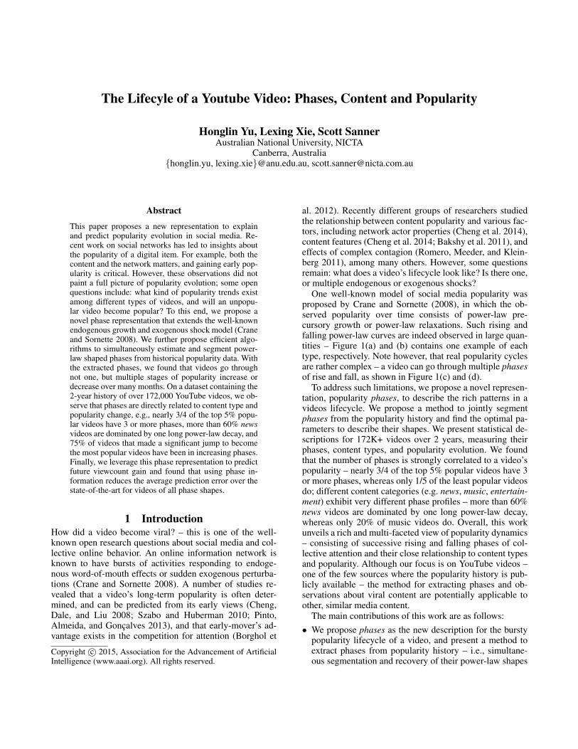
4.2 Phase evolution over timeHow long do phases last? Figure 4 examines the distribu-tion of phase durations, broken down into increasing and de-creasing phases, with popularity and category as co-variates.In Figure 4(a), we can see that popular videos tend to havelonger increasing phases, while the increasing phases forvideos in the least popular bins tend to be short. In Fig-ure 4(b), while there is a fair amount of long (≥ 160 days)decreasing phases across the entire popularity scale, theleast popular videos are still the most likely to have a longand dominant decreasing phase, this is consistent with Fig-ure 3(e). In (c) and (d), on the other hand, we can see thatthe probability of having longer phases of either type spreadover different categories. With music slightly more likelyto have longer increasing phases than other categories, andnews notably more likely to have a decreasing phase lastingmore than 320 days, consistent with Figure 3(f).

Are older videos forgotten? Since new phases tend to betriggered by external events, one may ask whether there areless activities and attention on older videos – in other words,are they forgotten? Surprisingly, the data says no. Figure 5plots the number of new phases that commence over the ageof a video (red curves broken down by phase types, in 15-

0 25 50 75 100popularity percentile (%)

05

10204080

160320735

dura

tion

ofph

ases

(a) increasing phase

0 25 50 75 100popularity percentile (%)

05

10204080

160320735 (b) decreasing phase

News

NonprTe

ch

GamesSpo

rt

AutosTra

vel

People

Animal

EducaEnte

r

Comed

HowtoFilm

Music

05

10204080

160320735

dura

tion

ofph

ases

(c) increasing phase

News

NonprTe

ch

GamesSpo

rt

AutosTra

vel

People

Animal

EducaEnte

r

Comed

HowtoFilm

Music

05

10204080

160320735 (d) decreasing phase

2%

5%

10%

30%

2%

5%

15%

Figure 4: Distribution of phase durations. X-axis: covari-ates – popularity percentile (20 values) and 15 content cate-gories. Y-axis: duration in days, with log-scaled bins. Inten-sity: the fraction of phases of a certain property (x) and dura-tion (y). We can see from (a) that many popular videos havelong and sustained (> 80 days) increasing phases, and from(b) that unpopular videos have longer decreasing phases(> 320 days). In (c), entertainment-related videos are morelikely to have long increasing phases. In (d), while newsvideos have by far the most amount of decreasing phasesover a year (also see Figure 3(f)), long decreasing phasesexist across all categories.

0 100 200 300 400 500 600 700 800

#days after uploading

0.001

0.01

0.1

1

frequ

ency

ofph

ase

trans

ition vex.inc.

vex.dec.cav.inc.cav.dec.

100

1000

averagedaily

viewcount

daily viewcount

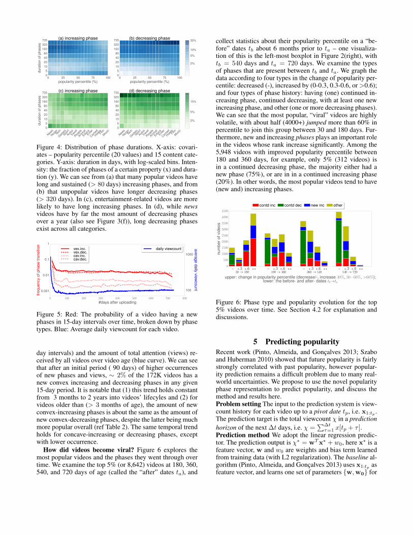
Figure 5: Red: The probability of a video having a newphases in 15-day intervals over time, broken down by phasetypes. Blue: Average daily viewcount for each video.

day intervals) and the amount of total attention (views) re-ceived by all videos over video age (blue curve). We can seethat after an initial period ( 90 days) of higher occurrencesof new phases and views, ∼ 2% of the 172K videos has anew convex increasing and decreasing phases in any given15-day period. It is notable that (1) this trend holds constantfrom 3 months to 2 years into videos’ lifecyles and (2) forvideos older than (> 3 months of age), the amount of newconvex-increasing phases is about the same as the amount ofnew convex-decreasing phases, despite the latter being muchmore popular overall (ref Table 2). The same temporal trendholds for concave-increasing or decreasing phases, exceptwith lower occurrence.

How did videos become viral? Figure 6 explores themost popular videos and the phases they went through overtime. We examine the top 5% (or 8,642) videos at 180, 360,540, and 720 days of age (called the “after” dates ta), and

collect statistics about their popularity percentile on a “be-fore” dates tb about 6 months prior to ta – one visualiza-tion of this is the left-most boxplot in Figure 2(right), withtb = 540 days and ta = 720 days. We examine the typesof phases that are present between tb and ta. We graph thedata according to four types in the change of popularity per-centile: decreased (-), increased by (0-0.3, 0.3-0.6, or >0.6);and four types of phase history: having (one) continued in-creasing phase, continued decreasing, with at least one newincreasing phase, and other (one or more decreasing phases).We can see that the most popular, “viral” videos are highlyvolatile, with about half (4000+) jumped more than 60% inpercentile to join this group between 30 and 180 days. Fur-thermore, new and increasing phases plays an important rolein the videos whose rank increase significantly. Among the5,948 videos with improved popularity percentile between180 and 360 days, for example, only 5% (312 videos) isin a continued decreasing phase, the majority either had anew phase (75%), or are in in a continued increasing phase(20%). In other words, the most popular videos tend to have(new and) increasing phases.

– +.3 +.6 ++ – +.3 +.6 ++ – +.3 +.6 ++ – +.3 +.6 ++

upper: change in popularity percentile (decrease/-, increase 30%, 30−60%, >60%);lower: the before- and after- dates tb→ta

0

500

1000

1500

2000

2500

3000

3500

4000

4500

num

bero

fvid

eos

30→ 180 180→ 360 360→ 540 540→ 720

contd inc contd dec new inc other

Figure 6: Phase type and popularity evolution for the top5% videos over time. See Section 4.2 for explanation anddiscussions.

5 Predicting popularityRecent work (Pinto, Almeida, and Goncalves 2013; Szaboand Huberman 2010) showed that future popularity is fairlystrongly correlated with past popularity, however popular-ity prediction remains a difficult problem due to many real-world uncertainties. We propose to use the novel popularityphase representation to predict popularity, and discuss themethod and results here.Problem setting The input to the prediction system is view-count history for each video up to a pivot date tp, i.e. x1:tp .The prediction target is the total viewcount χ in a predictionhorizon of the next ∆t days, i.e. χ =

∑∆tτ=1 x[tp + τ ].

Prediction method We adopt the linear regression predic-tor. The prediction output is χ∗ = wTx∗ + w0, here x∗ is afeature vector, w and w0 are weights and bias term learnedfrom training data (with L2 regularization). The baseline al-gorithm (Pinto, Almeida, and Goncalves 2013) uses x1:tp asfeature vector, and learns one set of parameters {w,w0} for

all videos. Our phase-informed method, first sorts a videointo one of eight subsets, according to (a) whether thereare more than 4 phases in x1:tp , intuitively this accountsfor the complexity and uncertainty of popularity evolutionfor this video, and (b) the shape of the last phase of theobservable viewcount (four types), this is useful informa-tion about how the phase and popularity will evolve. Wethen learn a separate predictor for each subset. When thelast phase is convex-decreasing, we add phase-extension, i.e.a(tp + τ)b + c, τ = 1, . . . ,∆t, as additional features.Performance metric and experimental setup To avoid be-ing dominated by the most popular videos that have or-ders of magnitude more views than others, we minimize anormalized mean-square-error (MSE). For each video, letxmax = max{x1:tp}, denote x = x/xmax, χ = χ/xmax.For a set of videos V , denote the normalized MSE as

ε =1

∆t|V|∑v∈V

(χ∗ − χ)2.

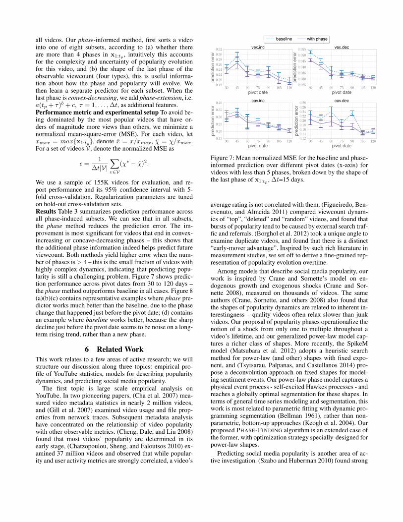
We use a sample of 155K videos for evaluation, and re-port performance and its 95% confidence interval with 5-fold cross-validation. Regularization parameters are tunedon hold-out cross-validation sets.Results Table 3 summarizes prediction performance acrossall phase-induced subsets. We can see that in all subsets,the phase method reduces the prediction error. The im-provement is most significant for videos that end in convex-increasing or concave-decreasing phases – this shows thatthe additional phase information indeed helps predict futureviewcount. Both methods yield higher error when the num-ber of phases is> 4 – this is the small fraction of videos withhighly complex dynamics, indicating that predicting popu-larity is still a challenging problem. Figure 7 shows predic-tion performance across pivot dates from 30 to 120 days –the phase method outperforms baseline in all cases. Figure 8(a)(b)(c) contains representative examples where phase pre-dictor works much better than the baseline, due to the phasechange that happened just before the pivot date; (d) containsan example where baseline works better, because the sharpdecline just before the pivot date seems to be noise on a long-term rising trend, rather than a new phase.

6 Related WorkThis work relates to a few areas of active research; we willstructure our discussion along three topics: empirical pro-file of YouTube statistics, models for describing popularitydynamics, and predicting social media popularity.

The first topic is large scale empirical analysis onYouTube. In two pioneering papers, (Cha et al. 2007) mea-sured video metadata statistics in nearly 2 million videos,and (Gill et al. 2007) examined video usage and file prop-erties from network traces. Subsequent metadata analysishave concentrated on the relationship of video popularitywith other observable metrics. (Cheng, Dale, and Liu 2008)found that most videos’ popularity are determined in itsearly stage, (Chatzopoulou, Sheng, and Faloutsos 2010) ex-amined 37 million videos and observed that while popular-ity and user activity metrics are strongly correlated, a video’s

30 45 60 75 90 105 120

pivot date

0.18

0.20

0.22

0.24

0.26

0.28

0.30

0.32

pred

ictio

ner

ror

vex.inc

baseline with phase

30 45 60 75 90 105 120

pivot date

0.025

0.030

0.035

0.040

0.045

0.050

0.055

pred

ictio

ner

ror

vex.dec

30 45 60 75 90 105 120

pivot date

0.15

0.20

0.25

0.30

0.35

0.40

pred

ictio

ner

ror

cav.inc

30 45 60 75 90 105 120

pivot date

0.120.140.160.180.200.220.240.260.28

pred

ictio

ner

ror

cav.dec

Figure 7: Mean normalized MSE for the baseline and phase-informed prediction over different pivot dates (x-axis) forvideos with less than 5 phases, broken down by the shape ofthe last phase of x1:tp , ∆t=15 days.

average rating is not correlated with them. (Figueiredo, Ben-evenuto, and Almeida 2011) compared viewcount dynam-ics of “top”, “deleted” and “random” videos, and found thatbursts of popularity tend to be caused by external search traf-fic and referrals. (Borghol et al. 2012) took a unique angle toexamine duplicate videos, and found that there is a distinct“early-mover advantage”. Inspired by such rich literature inmeasurement studies, we set off to derive a fine-grained rep-resentation of popularity evolution overtime.

Among models that describe social media popularity, ourwork is inspired by Crane and Sornette’s model on en-dogenous growth and exogenous shocks (Crane and Sor-nette 2008), measured on thousands of videos. The sameauthors (Crane, Sornette, and others 2008) also found thatthe shapes of popularity dynamics are related to inherent in-terestingness – quality videos often relax slower than junkvideos. Our proposal of popularity phases operationalize thenotion of a shock from only one to multiple throughout avideo’s lifetime, and our generalized power-law model cap-tures a richer class of shapes. More recently, the SpikeMmodel (Matsubara et al. 2012) adopts a heuristic searchmethod for power-law (and other) shapes with fixed expo-nent, and (Tsytsarau, Palpanas, and Castellanos 2014) pro-pose a deconvolution approach on fixed shapes for model-ing sentiment events. Our power-law phase model captures aphysical event process - self-excited Hawkes processes - andreaches a globally optimal segmentation for these shapes. Interms of general time series modeling and segmentation, thiswork is most related to parametric fitting with dynamic pro-gramming segmentation (Bellman 1961), rather than non-parametric, bottom-up approaches (Keogh et al. 2004). Ourproposed PHASE-FINDING algorithm is an extended case ofthe former, with optimization strategy specially-designed forpower-law shapes.

Predicting social media popularity is another area of ac-tive investigation. (Szabo and Huberman 2010) found strong

Table 3: Mean normalized MSE on different video subsets, with ∆t = 15, 30 days, tp = 60 days. ∗ denotes a significantimprovement (t-test, p < 0.05); † denotes relative error reduction > 5%.

∆t MethodPerformances on different subsets

#phase ≤ 4 (79.5% videos) #phase > 4 (20.5% videos)vex.inc vex.dec cav.inc cav.dec vex.inc vex.dec cav.inc cav.dec

15baseline 0.2450 ± 0.0103 0.0370 ± 0.0038 0.2745 ± 0.0447 0.2402 ± 0.0216 0.2555 ± 0.0105 0.1754 ± 0.0075 0.2722 ± 0.0095 0.2676 ± 0.0138phase 0.2232 ± 0.0093∗† 0.0337 ± 0.0037† 0.2614 ± 0.0432 0.1969 ± 0.0208∗† 0.2456 ± 0.0134 0.1745 ± 0.0072 0.2670 ± 0.0090 0.2654 ± 0.0124

30baseline 0.5013 ± 0.0386 0.0852 ± 0.0027 0.5953 ± 0.0562 0.5085 ± 0.0552 0.5146 ± 0.0288 0.3880 ± 0.0095 0.5719 ± 0.0388 0.5633 ± 0.0108phase 0.4642 ± 0.0373∗† 0.0771 ± 0.0011∗† 0.5734 ± 0.0598 0.4241 ± 0.0428∗† 0.4948 ± 0.0286 0.3865 ± 0.0106 0.5559 ± 0.0321 0.5594 ± 0.0118

Apr-0

7

Apr-0

7

May-0

7

May-0

7

Jun-

07

Jun-

070

100

200

300

400

500

600

700

daily

view

coun

t MSEbaseline = 7.1

MSEphase = 2.4

Jul-0

9

Aug-0

9

Aug-0

9

Sep-0

9

Sep-0

9

Oct-09

0

20

40

60

80

100

daily

view

coun

t MSEbaseline = 4.4

MSEphase = 0.6

Apr-0

7

Apr-0

7

May-0

7

May-0

7

Jun-

07

Jun-

070

20

40

60

80

100

120

140

daily

view

coun

t

MSEbaseline = 9.1

MSEphase = 4.3

Jan-

08

Feb-

08

Feb-

08

Mar-0

8

Mar-0

8

Mar-0

80

20

40

60

80

100

120

140

160

daily

view

coun

t MSEbaseline = 0.8

MSEphase = 4.8

dates (mmm-yy)

(a) ID: J4H8ihMJhow (b) ID: vf5B0STC KA (c) ID: x6wGQ1Afap4 (d) ID: hMEWt8jM9Y

Figure 8: (a)(b)(c): Three examples that phase-informed prediction performs much better than the baseline; (d): An exampleour method performs worse than the baseline (tp = 60,∆t = 30). Blue dots: daily viewcounts; Red curves: phase segmentsdetected; Green lines: indicating the pivot date.

linear correlations between (the log of) viewcount in thefirst week and those after the first month. (Pinto, Almeida,and Goncalves 2013) built on this insight and used multi-linear regression on the shape of popularity in the first fewdays to further improve medium-term prediction. Recently,(Cheng et al. 2014) showed that information cascades arepredictable (about whether or not they cross the median)with a set of rich descriptors about the network, timing,and users. This work proposes a detailed representation ofthe temporal dynamics, and showed that phases correlatewith video properties across the whole popularity scale, inaddition to the median (see Section 4). In addition, recentwork (Yu, Xie, and Sanner 2014) showed that a sudden risein popularity can be predicted with high accuracy from ex-ternal Twitter feeds, and popularity phases here is a new andnatural way to capture such sudden changes.

7 ConclusionWe proposed a novel representation, popularity phases, fordescribing the lifecycle of an online media item (i.e., aYouTube video in this investigation). Along with this repre-sentation, we devised a method for segmenting and estimat-ing power-law phases from viewcount traces and presentedobservations that uses phase history to explain content typeand long-term popularity. Furthermore, phase informationwas used in predicting future popularity, and our approachconsistently outperforms prediction approaches using view-count representations alone. Future work includes explicitmodeling of the underlying process with out-of-network in-put, and better prediction strategies for popularity. Overall,such multi-phase representation has potential to become a

tool for understanding the dynamics of other online media,such as hashtags and online memes, and we believe this is apromising direction for further uncovering the laws govern-ing online collective behavior.

Acknowledgements NICTA is funded by the Australian Gov-ernment as represented by the Department of Communicationsand the Australian Research Council (ARC) through the ICT Cen-tre of Excellence program. This research was supported in partby the National Computational Infrastructure (NCI) and ARCDP140102185. We would like to thank Xinhua Zhang for his helpon optimization.

References[Abisheva et al. 2014] Abisheva, A.; Garimella, V. R. K.; Garcia,

D.; and Weber, I. 2014. Who watches (and shares) what onyoutube? and when?: Using twitter to understand youtube view-ership. WSDM ’14, 593–602. New York, NY, USA: ACM.

[Ahmed et al. 2013] Ahmed, M.; Spagna, S.; Huici, F.; and Niccol-ini, S. 2013. A peek into the future: Predicting the evolution ofpopularity in user generated content. WSDM ’13, 607–616.

[Bakshy et al. 2011] Bakshy, E.; Hofman, J. M.; Mason, W. A.; andWatts, D. J. 2011. Everyone’s an influencer: quantifying influenceon twitter. In WSDM ’11, 65–74. ACM.

[Bellman 1961] Bellman, R. 1961. On the approximation of curvesby line segments using dynamic programming. Commun. ACM4(6):284–.

[Borghol et al. 2012] Borghol, Y.; Ardon, S.; Carlsson, N.; Eager,D.; and Mahanti, A. 2012. The untold story of the clones: content-agnostic factors that impact youtube video popularity. KDD ’12.

[Cha et al. 2007] Cha, M.; Kwak, H.; Rodriguez, P.; Ahn, Y.-Y.; andMoon, S. 2007. I tube, you tube, everybody tubes: analyzing theworld’s largest user generated content video system. In IMC ’07.

[Chatzopoulou, Sheng, and Faloutsos 2010] Chatzopoulou, G.;Sheng, C.; and Faloutsos, M. 2010. A first step towardsunderstanding popularity in youtube. In INFOCOM Workshops.

[Cheng et al. 2014] Cheng, J.; Adamic, L.; Dow, P. A.; Kleinberg,J. M.; and Leskovec, J. 2014. Can cascades be predicted? In WWW’14, 925–936.

[Cheng, Dale, and Liu 2008] Cheng, X.; Dale, C.; and Liu, J. 2008.Statistics and social network of youtube videos. In IWQoS ’08.

[Crane and Sornette 2008] Crane, R., and Sornette, D. 2008. Ro-bust dynamic classes revealed by measuring the response functionof a social system. PNAS 105(41):15649–15653.

[Crane, Sornette, and others 2008] Crane, R.; Sornette, D.; et al.2008. Viral, quality, and junk videos on youtube: Separating con-tent from noise in an information-rich environment. In AAAI SpringSymposium: Social Information Processing, 18–20.

[Figueiredo, Benevenuto, and Almeida 2011] Figueiredo, F.; Ben-evenuto, F.; and Almeida, J. M. 2011. The tube over time: Charac-terizing popularity growth of youtube videos. In WSDM ’11.

[Gill et al. 2007] Gill, P.; Arlitt, M.; Li, Z.; and Mahanti, A. 2007.Youtube traffic characterization: a view from the edge. In IMC’07.

[Golub and Pereyra 2003] Golub, G., and Pereyra, V. 2003. Sep-arable nonlinear least squares: the variable projection method andits applications. Inverse problems 19(2):R1.

[Keogh et al. 2004] Keogh, E. J.; Chu, S.; Hart, D.; and Pazzani,M. 2004. Segmenting time series: A survey and novel approach.In Data Mining In Time Series Databases, volume 57. 1–22.

[Matsubara et al. 2012] Matsubara, Y.; Sakurai, Y.; Prakash, B. A.;Li, L.; and Faloutsos, C. 2012. Rise and fall patterns of informationdiffusion: Model and implications. KDD ’12.

[Pinto, Almeida, and Goncalves 2013] Pinto, H.; Almeida, J. M.;and Goncalves, M. A. 2013. Using early view patterns to predictthe popularity of youtube videos. In WSDM ’13, 365–374.

[Rabiner 1989] Rabiner, L. 1989. A tutorial on hidden markovmodels and selected applications in speech recognition. Proceed-ings of the IEEE 77(2):257–286.

[Romero, Meeder, and Kleinberg 2011] Romero, D. M.; Meeder,B.; and Kleinberg, J. 2011. Differences in the mechanics of in-formation diffusion across topics: idioms, political hashtags, andcomplex contagion on twitter. In WWW ’11, 695–704.

[Sornette and Helmstetter 2003] Sornette, D., and Helmstetter, A.2003. Endogenous versus exogenous shocks in systems with mem-ory. Physica A 318(3-4):577 – 591.

[Szabo and Huberman 2010] Szabo, G., and Huberman, B. A.2010. Predicting the popularity of online content. Commun. ACM53(8):80–88.

[Tsytsarau, Palpanas, and Castellanos 2014] Tsytsarau, M.; Pal-panas, T.; and Castellanos, M. 2014. Dynamics of news eventsand social media reaction. KDD ’14.

[Xie et al. 2011] Xie, L.; Natsev, A.; Kender, J. R.; Hill, M.; andSmith, J. R. 2011. Visual memes in social media: Tracking real-world news in youtube videos. In ACM Multimedia, 53–62.

[Yang and Leskovec 2011] Yang, J., and Leskovec, J. 2011. Pat-terns of temporal variation in online media. In WSDM ’11.

[Yu, Xie, and Sanner 2014] Yu, H.; Xie, L.; and Sanner, S. 2014.Twitter-driven youtube views: Beyond individual influencers. MM’14, 869–872. New York, NY, USA: ACM.

[Zhu et al. 1997] Zhu, C.; Byrd, R. H.; Lu, P.; and Nocedal, J.1997. Algorithm 778: L-BFGS-B: Fortran subroutines for large-scale bound-constrained optimization. ACM Trans. Math. Softw.23(4):550–560.

A The PHASE-FINDING algorithmA.1 Estimating a generalized power-law phaseIn this work, we use sum-of-squares loss in problem (4). De-note the relative time and duration in a phase as time elapsedsince the end of the previous phase t = t − ts + 1 andT = te − ts + 1.

min{a,b,c}

E{x[ts : te]; a, b, c}

=1

2

T∑t=1

(atb

+ c− x[t])2 (5)

Notice that this loss function is differentiable everywhere,but non-convex in {a, b, c} – it can be optimized with ageneral unconstrained optimization technique such as New-ton’s method, but it will be prone to local minima, and slowto converge. We adopt a technique called variable projec-tion (Golub and Pereyra 2003) to address this problem. Thebasic idea is to separate the nonlinear parameter b and thelinear parameter a, c, by re-writing the loss function as fol-lows.

E =1

2

T∑t=1

(atbi + c− x[t])2 =

1

2||Φ(t) · β − x||2 (6)

where

Φ(t) =

1b, 1

2b, 1

...

T b, 1

, β =

[a

c

](7)

Φ(t) includes the nonlinear parameter b, and β includesthe linear parameters a and c. Given b, there is a uniqueminimum for the quadratic equation (6), with a, c given bythe following closed-form via the Moore–Penrose pseudoin-verse: [

a

c

]= (Φ(t)TΦ(t))−1Φ(t)Tx (8)

Equation (8) is a necessary condition of the optimal solutionof Equation (6). Substituting a and c by it, the loss functionbecomes:

E =1

2||Φ(t)(Φ(t)TΦ(t))−1Φ(t)Tx− x||2 (9)

Now, we have reduced the parameter space from {a, b, c} ∈R3 to b ∈ R. And the optimal solutions of Equation 9 is thesame with that of Equation (6).Implementation and solution quality. We use the L-BFGS-B algorithm (Zhu et al. 1997) to find a solution of this non-linear objective. We search over the two temporal direc-tions in Eq (2) and take the direction with a small mean-square-error. We observed significant improvement in speedand solution quality with the variable projection technique,consistent with the original proposal (Golub and Pereyra2003). We also normalize x1:T into [0, 100] before runningthe phase-finding algorithm to be on the same order of mag-nitude with time stamp t – thus avoiding numerical issues

in fitting a handful to a few million daily views. In ad-dition, we employ the following initialization technique tostart from a good “guess” of b — we use t = 1 with eachobservation t = 2, . . . , T to solve for a value b by assum-ing each pair exactly follows power-law “x = atb” (with-out c), and then average these estimates as the initial value3.As an initial validation for the solution quality of this curve-fitting problem, we generate 500 synthetic power-law curves(of length 200) with parameters randomly chosen from uni-form distributions a ∼ U [−100, 100], b ∼ U [−2, 2], andc ∼ U [−500, 500], and a and b bounded away from zeroto avoid degenerate cases (|a| > 3, |b| > 0.1). We op-timize Equation (9), and observed the relative fitting errorin each coefficient (Ea = |a∗ − a|/|a|, with the corre-sponding confidence intervals) as: Ea = (1.8± 0.3)×10−3,Eb = (1.1± 0.6)×10−5 Ec = (1.8± 0.3)×10−3.

A.2 Simultaneous fitting and segmentationA bruce-force enumeration approach to the joint segmen-tation and curve-fitting problem (3) will have a complexityexponential in T , the sequence length. Fortunately problem(3) is in a form suitable for induction with dynamic pro-gramming. We describe the algorithm in three stages, similarto (but extending) the description of the well-known Viterbidecoding algorithm (Rabiner 1989) with embedded curve-fitting.

As in problem (3), denote 1 ≤ t′ ≤ T as the current posi-tion in the recursion, n′ as the number of optimal segmentsup to position t′, and a shorthand E∗(t′) for the lowest seg-mentation and fitting error (under any segmentation) for thesubsequence x1:t′

E∗(t′) = minE{x1:t′ , ρ1:n′ , θ1:n′} (10)

here the minimization is done over {n′, ts[1 : n′], θ1:n′}.In order to retrieve an optimal segmentation, we need to

keep track of arguments that minimize Equation (10) foreach t′. This is done via a pointer for each t′ containing thestarting position of the last phase and its parameters.

δ(t′) = {ts∗n′ , θ∗n′} (11)

The complete procedure for finding the best segmentationand their power-law fits is as follows:

Stage 1 Initialization:

for t = 1, 2, E∗(t) = 0 (12)δ(t) = ∅

The reason we initialize a cost of zero and an empty pa-rameter set for the first two positions (instead of onlyfor t = 1 as the Viterbi algorithm) is that the general-ized power-law curve has three free parameters, and hencetakes at least three observations to fit.

Stage 2 Recursion:

E∗(t′) = mintsn′ ,θn′

{E∗(ten′−1) + E(x[tsn′ : t′], θn′)} (13)

3This initialization heuristic is documented in thepower2start() function of Matlab curve-fitting toolbox.

The step above computes the cumulative minimum error,for t′ = 3, 4, . . . , T . This is done by searching for an opti-mal starting point tsn′ = 1, 2, . . . , t′, for the current phasethat ends at t′, and obtaining optimal parameter θ∗n′ thatminimizes fitting error on subsequence x[tsn′ : t′] for eachtsn′ , using the PHASE-FITTING algorithm in Section A.1.We also populate the backtracking pointers:

δ(t′) = arg mintsn′ ,θn′

{E∗(ten′−1) + E(x[tsn′ : t′], θn′)} (14)

Stage 3 Backtracking: The set of segmentation parametersS∗ = {n∗, ts∗1:n, θ

∗1:n} is obtained using recursion:

• Initialize S∗ ← δ(T ), t′ ← tsn′ , n∗ ← 1;• Recurse S∗ ← S∗ ∪ δ(t′), t′ ← tsn′ , n∗ ← n∗ + 1;• Terminate S∗ ← S∗ ∪ n∗.

How to avoid over-fitting Every three observations willprovide a unique solution for the curve-fitting problem (4)with a set of a, b, c – this can easily lead to over-fitting byover segmentation. We introduce a segment regularizer, byadding a penalty constant η to every new segment introducedby the algorithm. That is, the objective for problem (3) ismodified as:

E{x1:T , ρ1:n, θ1:n} =

n∑i=1

Ei{x[tsi : tei ], θi}+ (n− 1)η

(15)

Minimizing the objective is still done with dynamic pro-gramming, by simply adding η to the iteration step (13),

E∗(t′) = mintsn′ ,θn′

E∗(ten′−1) + E{x[tsn′ : t′], θn′}+ η (16)

and also modify step (14) accordingly.Implementation and solution quality. Hyper-parameter ηcontrols the trade-off between fitting each phase well, andhaving a reasonable number of phases. To calibrate thevalue of η, we invite 6 people to choose their preferred seg-mentation for a random sample of 210 videos. This is doneon a web interface, screenshot of which is at project web-site??. The labelers have about 72% agreement on the phaseboundaries (that are ± 2 days of each other). Then we do aline search on η with the set of agreed boundaries and foundwhen η = 2.3, the algorithm achieves the highest F1-score0.707 with recall = 0.779 and precition = 0.648.

The running time for step (13) above isO(TΓ(T )), whereO(T ) is the time for searching over tsn′ and Γ(T ) is the T -dependent time complexity of power-law curve fitting andfinding θ∗n′ . The complexity of this entire dynamic program-ming algorithm is hence O(T 2Γ(T )). We implemented thisalgorithm in C++, the throughput for finding phases for one-year long viewcount sequences is about 400 per CPU perhour.