The Lie theory approach to special functions

Willard MillerUniversity of Minnesota

November 5, 2010

Contents

0.1 Abstract and introduction . . . . . . . . . . . . . . . . . . . . 2

1 Preliminaries 41.1 Definition of a group . . . . . . . . . . . . . . . . . . . . . . . 41.2 Lie groups and algebras, transformation groups . . . . . . . . 51.3 Group representations . . . . . . . . . . . . . . . . . . . . . . 91.4 Orthogonality relations for finite groups . . . . . . . . . . . . . 101.5 Invariant measures on Lie groups . . . . . . . . . . . . . . . . 101.6 Orthogonality relations for compact Lie groups . . . . . . . . 101.7 The Peter-Weyl theorem . . . . . . . . . . . . . . . . . . . . . 11

2 Special functions as matrix elements 122.1 A classical example: The rotation group and spherical har-

monics . . . . . . . . . . . . . . . . . . . . . . . . . . . . . . . 132.2 Matrix elements of some other group representations: SL(2,C),

SL(2,R), SU(2) . . . . . . . . . . . . . . . . . . . . . . . . . . 16

3 Symmetries of differential equations 203.1 The wave equation and Gaussian hypergeometric functions . . 213.2 Canonical equations for generalized hypergeometric functions.

Introduction to Gel’fand theory . . . . . . . . . . . . . . . . . 26

4 Symmetry characterization of variable separation for theHelmholtz and Schrodinger equations 284.1 Constuction of separable coordinate systems for spheres and

Euclidean space . . . . . . . . . . . . . . . . . . . . . . . . . . 304.2 Example of separation of variables: A “magic” potential on

the n-sphere . . . . . . . . . . . . . . . . . . . . . . . . . . . . 324.2.1 Orthogonal bases of separable solutions . . . . . . . . . 36

1

4.2.2 Relations between bases on the sphere . . . . . . . . . 40

5 Clebsch-Gordan coefficients and orthogonal polynomials 44

6 Harmonic analysis and lattice subgroups 486.1 Harmonic analysis: windowed Fourier transforms . . . . . . . 486.2 Harmonic analysis: continuous wavelets . . . . . . . . . . . . . 496.3 Harmonic analysis: discrete wavelets and the multiresolution

structure . . . . . . . . . . . . . . . . . . . . . . . . . . . . . . 51

7 Significant research opportunities and challenges 57

0.1 Abstract and introduction

These notes describe some of the most important interrelationships betweenthe theory of Lie groups and algebras, and special functions, with a strongemphasis on results obtained in the 50 years after the publication of theBateman Project. An informal justification for this treatment is that mostfunctions commonly called “ special ” obey symmetry properties that are bestdescribed via group theory (the mathematics of symmetry). In particular,those special functions that arise as explicit solutions of the partial differentialequations of mathematical physics, such as via separation of variables, canbe characterized in terms of their transformation properties under the Liesymmetry groups and algebras of the differential equations. (The same ideasextend to difference and q-difference equations.) We shall treat, briefly, thefollowing topics:

1. Special functions as matrix elements of Lie group representations. (ad-dition theorems, orthogonality relations)

2. Special functions as basis functions for Lie group representations (gen-erating functions)

3. Special functions as solutions of Laplace-Beltrami eigenvalue problems(with potential) via separation of variables.

4. Special functions as Clebsch-Gordan coefficients for the reduction oftensor products of irreducible group representations (the motivationfor Wilson polynomials).

2

In practice, the first two items involve hypergeometric functions predomi-nantly and are special cases of the third item. The group theoretic basis forvariable separation allows treatment of non-hypergeometric functions, suchas those of Lame and Heun. The last item provides an important motivationfor the constuction of the Askey-Wilson polynomials.

I conclude with a brief examination of special functions (or functionsthat deserve to be called “special”) that arise when one restricts certainirreducible Lie group representations to a discrete lattice subgroup. The twomost important examples are an irreducible representation of the Heisenberggroup (and its relation to the windowed Fourier transform, the Weil-Brezin-Zak transform and theta functions), and an irreducible representation ofthe affine group (and its relation to the continuous and discrete wavelettransforms). We briefly describe the properties of the Daubechies familyof scaling functions, a very modern family of “special” functions arising assolutions of two-scale difference equations.

I am omitting some topics of equal or greater importance than the above,such as quantum groups, Askey-Wilson polynomials, Koornwinder’s additiontheorems for disk and Jacobi polynomials and other polynomials transform-ing under group actions, special functions related to root systems of semi-simple Lie algebras, Dunkl’s theory of special funtions related to discretesymmetries on spheres, etc., because they will be treated by other partici-pants in this meeting, for lack of time, or lack of expertise.

3

Chapter 1

Preliminaries

A group is an abstract mathematical entity which expresses the intuitiveconcept of symmetry. Here I collect some standard definitions and resultsfrom classical group theory.

1.1 Definition of a group

A group is an abstract mathematical entity which expresses the intuitiveconcept of symmetry.

Definition 1 A group G is a set of objects {g, h, k, · · · } (not necessarilycountable) together with a binary operation which associates to any orderedpair of elements g, h in G a third element gh. the binary operation (calledgroup multiplication) is subject to the following requirements:

1. There exists an element e in G called the identity element such thatge = eg = g for all g ∈ G.

2. For every g ∈ G there exists in G an inverse element g−1 such thatgg−1 = g−1g = e.

3. Associative law. The identity (gh)k = g(hk) is satisfied for all g, h, k ∈G.

4

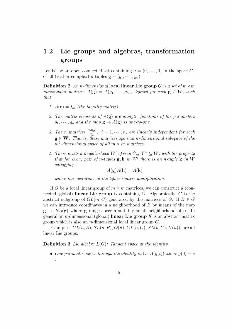
1.2 Lie groups and algebras, transformation

groups

Let W be an open connected set containing e = (0, · · · , 0) in the space Cnof all (real or complex) n-tuples g = (g1, · · · , gn).

Definition 2 An n-dimensional local linear Lie group G is a set of m×mnonsingular matrices A(g) = A(g1, · · · , gn), defined for each g ∈ W , suchthat

1. A(e) = Im (the identity matrix)

2. The matrix elements of A(g) are analytic functions of the parametersg1, · · · , gn and the map g→ A(g) is one-to-one.

3. The n matrices ∂A(g)∂gj

, j = 1, · · · , n, are linearly independent for each

g ∈W. That is, these matrices span an n-dimensional subspace of them2-dimensional space of all m×m matrices.

4. There exists a neighborhood W ′ of e in Cn, W′ ⊆ W , with the property

that for every pair of n-tuples g,h in W ′ there is an n-tuple k in Wsatisfying

A(g)A(h) = A(k)

where the operation on the left is matrix multiplication.

If G be a local linear group of m×m matrices, we can construct a (con-nected, global) linear Lie group G containing G. Algebraically, G is theabstract subgroup of GL(m,C) generated by the matrices of G. If B ∈ Gwe can introduce coordinates in a neighborhood of B by means of the mapg → BA(g) where g ranges over a suitably small neighborhood of e. Ingeneral an n-dimensional (global) linear Lie group K is an abstract matrixgroup which is also an n-dimensional local linear group G.

Examples: GL(n,R), SL(n,R), O(n), GL(n,C), SL(n,C), U(n)), are alllinear Lie groups.

Definition 3 Lie algebra L(G): Tangent space at the identity.

• One parameter curve through the identity in G: A(g(t)) where g(0) = e.

5

• L(G) consists of all matrices A = ddtA(g(t))|t=0 as g runs over all

differentiable curves through the origin.

• L(G) is a vector space: if g(t) → A and h(t) → B and α, β scalars,then g(αt)h(βt)→ αA+ βB.

• L(G) is closed under commutation: if g(t) → A and h(t) → B theng(t)h(t)g−1(t)h−1(t) = k(t2)→ [A,B] = AB − BA.

• Properties of the commutator:

[A,B] = −[B,A] (skew symmetry)

[αA+ βB, C] = α[A, C] + β[B, C], α, β scalars (linearity)

[[A,B], C] + [[B, C],A] + [[C,A],B] = 0, (Jacobi identity).

Holds automatically for matrix Lie algebras.

• Basic relation between Lie algebra and local Lie group: A(t) is a one-parameter subgroup of G, i.e.,

A(t) ∈ G,A(t1)A(t2) = A(t1+t2)⇐⇒ A(t) = exp(tA) =∞∑j=0

(tA)j

j!, A ∈ L(G).

Definition 4 Action of a Lie group as a Lie transformation group: Let Gbe a local Lie group and M a local coordinate manifold. G acts as a localtransformatin group on M if there is an analytic mapping M× g → M :x× g→ xg such that

(xg)h = x(gh), xe = x, g,h ∈ G, x ∈M.

We can transfer this action to functions f(x) onM by defining operatorsT (g) such that

T (g)f(x) = f(xg),

6

or, more generally,T (g)f(x) = ν(g, x)f(xg),

where the multiplier ν(g, x) satisfies ν(gh, x) = ν(g, x)ν(h, xg). These oper-ators satify the (local) group law

T (g)T (h) = T (gh).

By transferring this action to the tangent space at the identity,

T (A)f(x) =d

dtT (exp tA)f(x)|t=0,

one gets a realization of L(G) by first order linear differential operators:

T (αA+ βB) = αT (A) + βT (B),

T ([A,B]) = [T (A), T (B)] = T (A)T (B)− T (B)T (A).

EXAMPLE: ax+ b or “affine” group.

• g = (a, b), a > 0, b real. gh = (a, b) · (c, d) = (ac, ad+ b).

• Linear Lie group: g ⇔ A(g), such that A(g)A(h) = A(gh).

(a, b) = g⇔ A(g) =

(a b0 1

).

• A basis for the two-dimensional Lie algebra is given by the matrices

L1 =d

dt

(et 00 1

)|t=0 =

(1 00 0

)

L2 =d

dt

(1 t0 1

)|t=0 =

(0 10 0

),

with commutation relation

[L1,L2] = L2.

7

• An action on the real line given by

xg =x− ba

or

T (g)f(x) = f(x− ba

).

• The induced differential operators that represent the Lie algebra actingon functions of x are

T (L1) = L1 = −x ddx, T (L2) = L2 = − d

dx, [L1, L2] = L2.

EXAMPLE: The (three-dimensional real) Heisenberg group HR

•

HR =

g(x1, x2, x3) =

1 x1 x3

0 1 x2

0 0 1

: xi ∈ R

.

• This is a subgroup of GL(3, R) with group product

g(x1, x2, x3) · g(y1, y2, y3) = g(x1 + y1, x2 + y2, x3 + y3 + x1y2).

The identity element is the identity matrix g(0, 0, 0) and g(x1, x2, x3)−1 =g(−x1,−x2, x1x2 − x3).

• A basis for the three-dimensional Lie algebra is given by the matrices

L1 =d

dt

1 t 00 1 00 0 1

|t=0 =

0 1 00 0 00 0 0

L2 =

d

dt

1 0 00 1 t0 0 1

|t=0 =

0 0 00 0 10 0 0

L3 =

d

dt

1 0 t0 1 00 0 1

|t=0 =

0 0 10 0 00 0 0

with commutation relations

[L1,L2] = L3, [L1,L3] = [L2,L3] = 0.

8

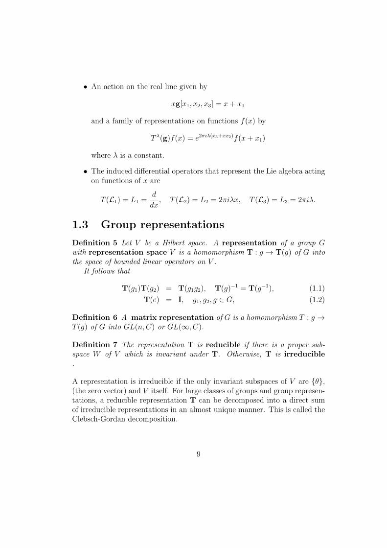
• An action on the real line given by

xg[x1, x2, x3] = x+ x1

and a family of representations on functions f(x) by

T λ(g)f(x) = e2πiλ(x3+xx2)f(x+ x1)

where λ is a constant.

• The induced differential operators that represent the Lie algebra actingon functions of x are

T (L1) = L1 =d

dx, T (L2) = L2 = 2πiλx, T (L3) = L3 = 2πiλ.

1.3 Group representations

Definition 5 Let V be a Hilbert space. A representation of a group Gwith representation space V is a homomorphism T : g → T(g) of G intothe space of bounded linear operators on V .

It follows that

T(g1)T(g2) = T(g1g2), T(g)−1 = T(g−1), (1.1)

T(e) = I, g1, g2, g ∈ G, (1.2)

Definition 6 A matrix representation of G is a homomorphism T : g →T (g) of G into GL(n,C) or GL(∞, C).

Definition 7 The representation T is reducible if there is a proper sub-space W of V which is invariant under T. Otherwise, T is irreducible.

A representation is irreducible if the only invariant subspaces of V are {θ},(the zero vector) and V itself. For large classes of groups and group represen-tations, a reducible representation T can be decomposed into a direct sumof irreducible representations in an almost unique manner. This is called theClebsch-Gordan decomposition.

9

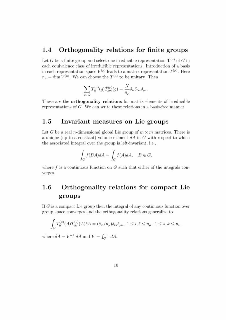
1.4 Orthogonality relations for finite groups

Let G be a finite group and select one irreducible representation T(µ) of G ineach equivalence class of irreducible representations. Introduction of a basisin each representation space V (µ) leads to a matrix representation T (µ). Herenµ = dimV (µ). We can choose the T (µ) to be unitary. Then∑

g∈G

T(µ)i` (g)T (ν)

sm (g) =N

nµδisδ`mδµν .

These are the orthogonality relations for matrix elements of irreduciblerepresentations of G. We can write these relations in a basis-free manner.

1.5 Invariant measures on Lie groups

Let G be a real n-dimensional global Lie group of m×m matrices. There isa unique (up to a constant) volume element dA in G with respect to whichthe associated integral over the group is left-invariant, i.e.,∫

G

f(BA)dA =

∫G

f(A)dA, B ∈ G,

where f is a continuous function on G such that either of the integrals con-verges.

1.6 Orthogonality relations for compact Lie

groups

If G is a compact Lie group then the integral of any continuous function overgroup space converges and the orthogonality relations generalize to∫

G

T(µ)i` (A)T

(ν)sk (A)δA = (δis/nµ)δ`kδµν , 1 ≤ i, ` ≤ nµ, 1 ≤ s, k ≤ nν ,

where δA = V −1 dA and V =∫G

1 dA.

10

1.7 The Peter-Weyl theorem

Let L2(G) be the space of all functions on the compact goup G which are(Lebesgue) square-integrable:

L2(G) = {f(A) :

∫G

|f(A)|2δA <∞}.

With respect to the inner product

〈f1, f2〉 =

∫G

f1(A)f2(A)δA.

L2(G) is a Hilbert space. Let

ϕ(µ)ij (A) = n1/2

µ T(µ)ij (A).

It follows from the orthogonality relations that {ϕ(µ)ij }, where 1 ≤ i, j ≤ nµ

and µ ranges over all equivalence classes of irreducible representations, formsan ON set in L2(G).

Theorem 1 (Peter-Weyl). If G is a compact linear Lie group, the set {ϕ(µ)ij }

is an ON basis for L2(G).

11

Chapter 2

Special functions as matrixelements

Let T be a representation of the Lie group G on the Hilbert space V andlet {vn} be an ON basis for V . (Here {vn} is typically chosen so that it hassimple transformation properties with respect to the subgroups in some chainG ⊃ G1 ⊃ G2 ⊃ · · · ⊃ {e}.) Then the matrix elements of the operators T(g)with respect to this basis satisfy the addition theorem

Tkm(g1g2) =∑j

Tkj(g1)Tjm(g2), g1, g2 ∈ G.

If T is a unitary representation then these matrices are unitary:

Tmn(g−1) = Tnm(g).

For important classes of groups G and bases {vn} these matrix elements arefamiliar special functions. With respect to the inner product on the Hilbertspace, the matrix elements can be expressed as

Tkm(g) =< T(g)vm, vk >,

which for function space models ot T may provide an integral representationof the matrix elements.

12

2.1 A classical example: The rotation group

and spherical harmonics

A very important example of the orthogonality relations for compact lin-ear Lie groups and the Peter-Weyl theorem is the rotation group SO(3) =SO(3, R). This case was already treated in the Bateman project. Recall thatSO(3) has a convenient realization as the group of all 3× 3 real matrices Asuch that AtA = I3 and detA = 1. This is the natural realization of SO(3)as the group of all rotations in R3 which leave the origin fixed. One conve-nient parametrization of SO(3) is in terms of the Euler angles. A rotationthrough angle ϕ about the z axis is given by

Rz(ϕ) =

cosϕ − sinϕ 0sinϕ cosϕ 0

0 0 1

∈ SO(3)

and rotations through angle ϕ about the x and y axis are given by

Rx(ϕ) =

1 0 00 cosϕ − sinϕ0 sinϕ cosϕ

∈ SO(3),

Ry(ϕ) =

cosϕ 0 sinϕ0 1 0

− sinϕ 0 cosϕ

∈ SO(3),

respectively. Differentiating each of these curves in SO(3) with respect to ϕand setting ϕ = 0 we find the following linearly independent matrices in thetangent space at the identity:

Lz =

0 −1 01 0 00 0 0

, Lx =

0 0 00 0 −10 1 0

, Ly =

0 0 10 0 0−1 0 0

.

One can check from the definition AtA = E3 that the tangent space at theidentity is at most three-dimensional, so the matrices Lx, Ly, Lz form a basisfor this space.

The Euler angles ϕ, θ, ψ for A ∈ SO(3) are given by

A(ϕ, θ, ψ) = Rz(ϕ)Rx(θ)Rz(ψ)

13

=

cosϕ cosψ − sinϕ sinψ cos θ sinϕ cosψ + cosϕ sinψ cos θ sinψ sin θ− cosϕ sinψ − sinϕ cosψ cos θ sinϕ sin θ − sinϕ sinψ + cosϕ cosψ cos θ − cosϕ sin θ

cosψ sin θ cos θ

,

dA = sin θdϕdθdψ.

Since SO(3) is compact, dA is both left- and right-invariant. The volume ofSO(3) is

VSO(3) =

∫SO(3)

dA =

∫ 2π

0

dψ

∫ 2π

0

dϕ

∫ π

0

sin θdθ = 8π2.

The irreducible unitary representations of SO(3) are denoted T(`), ` = 0, 1, 2, · · · ,where dim T(`) = 2`+1. Expressed in terms of an ON basis for the represen-tation space V (`) consisting of simultaneous eigenfunctions for the operatorsT(`)(Rz(ϕ)), the matrix elements are

T `km(ϕ, θ, ψ) = ik−m[

(`+m)!(`−k)!(`+k)!(`−m)!

]1/2

ei(kϕ+mψ) [sin θ]m−k(1+cos θ)`+k−m

2`Γ(m−k+1) 2F1

(−`,−km− 1

; cos θ−1cos θ+1

)= ik−m

[(`+m)!(`−k)!(`+k)!(`−m)!

]1/2

ei(kϕ+mψ)P−k,m` (cos θ),

where −` ≤ k,m ≤ `. Here 2F1

(a, bc

, x

)is the Gaussian hypergeometric

function and Γ(z) is the gamma function. A generating function for thematrix elements is

g(A, z) =(βz + α)`−m(αz − β)`+m

[(`−m)!(`+m)!]1/2=∑k=−`

T `km(A)(−1)k−mz`+k

[(`− k)!(`+ k)!]1/2

where

α = ei(ϕ+ψ)/2 cosθ

2, β = iei(φ−ψ)/2 sin

θ

2.

The group property

T `km(A1A2) =∑j=−`

T `kj(A1)T `jm(A2)

defines an addition theorem obeyed by the matrix elements. The unitaryproperty of the operator T(`)(A) implies

T `km(A−1) = T `mk(A),

14

or in Euler angles,

(−1)m−kP−k,m` (cos θ) =(`+ k)!(`−m)!

(`− k)!(`+m)!P−m,k` (cos θ).

Also, |T `km(A)| ≤ 1 or

|P−k,m` (cos θ)| ≤[

(`+ k)!(`−m)!

(`+m)!(`− k)!

]1/2

, 0 ≤ θ ≤ π.

The matrix elements T `om(ϕ, θ, ψ), are proportional to the spherical harmonicsY m` (θ, ψ). Indeed

T `om(ϕ, θ, ψ) = im(

4π

2`+ 1

)1/2

Y m` (θ, ψ) = im

[(`−m)!

(`+m)!

]1/2

Pm` (cos θ)eimψ

where the Pm` (cos θ) are the associated Legendre functions. Moreover,

T `oo(ϕ, θ, ψ) = P`(cos θ)

where P`(cos θ) is the Legendre polynomial.Orthogonality relations:∫

SO(3)

T `km(A)T `′k′m′(A)dA =

8π2

2`+ 1δkk′δmm′δ``′ .

Thus∫ 2π

0

dψ

∫ 2π

0

dϕ

∫ π

0

dθ T `km(ϕ, θ, ψ)T `′k′m′(ϕ, θ, ψ) sin θ =

8π2

2`+ 1δkk′δmm′δ``′ .

The ψ and ϕ integrations are trivial, while the θ integration gives∫ π

0

P k,m` (cos θ)P k,m

`′ (cos θ) sin θdθ =2

2`+ 1

(`− k)!(`−m)!

(`+ k)!(`+m)!δ``′ .

For k = m = 0 these are the orthogonality relations for the Legendrepolynomials. (Note: By definition, P 0,−m

` (cos θ) = Pm` (cos θ), P 0,0

` (cos θ) =P`(cos θ), where Pm

` , P` are Legendre functions.)By the Peter-Weyl theorem, the functions

ϕ`km(ϕ, θ, ψ) = (2`+ 1)1/2T `km(ϕ, θ, ψ),−` ≤ k,m ≤ `, ` = 0, 1, 2, · · ·

15

constitute an ON basis for L2(SO(3)). If f ∈ L2(SO(3)) then

f(ϕ, θ, ψ) =∞∑`=0

∑k,m=−`

a`kmϕ`km(ϕ, θ, ψ)

where

a`km = (f, ϕ`km) =1

8π2

∫ 2π

0

dψ

∫ 2π

0

dϕ

∫ π

0

dθ ×

×f(ϕ, θ, ψ)ϕ`km(ϕ, θ, ψ) sin θ.

2.2 Matrix elements of some other group rep-

resentations: SL(2,C), SL(2,R), SU(2)

Example 1 SL(2,C).

SL(2, C) =

{A =

(a bc d

): a, b, c, d ∈ C, det(A) = 1

}.

L (SL(2, C)) = s`(2, C) =

{A =

(α βγ δ

): α, β, γ, δ ∈ C, trace(A) = 0

}.

Basis for Lie algebra: L+, L−, L3

[L3, L±] = ±L±, [L+, L−] = 2L3.

L+ =

(0 −10 0

), L− =

(0 0−1 0

), L3 =

(12

00 −1

2

).

Finite-dimensional representations

Tu(A)f(z) = (bz + d)2uf(az + c

bz + d), 2u = 0, 1, 2, · · · .

Basis for representation space:

fj(z) = zj, j = 0, 1, · · · , 2u.

Matrix elements: Tu(A)fj(z) =∑2u

`=oD`j(A)f`(z)

(az + c)j(bz + d)2u−j =2u∑`=0

D`j(A)z`

16

D`j(A) =a`d2u−jcj−`j!

`!(j − `)! 2F1

(−` −2u+ j

j − `+ 1;bc

ad

).

Addition theorem:

D`j(AB) =2u∑k=0

D`k(A)Dkj(B), `, j = 0, 1, · · · , 2u.

Restrict to subgroup SU(2) and use Euler angles to parametrize group ele-ments. Then D`j(φ, θ, ψ) is a Wigner D-function and D0m(φ, θ, ψ) ∼ Y m

` (θ, φ)is a spherical harmonic, where ` = 2u. With respect to the normalized basis,the matrix elements are unitary: Uu

nm(A−1) = Uumn(A).

Note: The addition theorem shows that for fixed ` the matrix elementD`j(A) transforms under right multiplication bt B exactly as the bais functionfj. passing to the Lie algebra action we see that the addition theorem for the

2F1 polynomials is obtained from exponentiating the differential recurrencerelations Eβγ, Eβγ for the

2F1

(α, βγ

; z

)where Eβγ raises the β and γ parameters by one and Eβγ lowers the β andγ parameters by one.

Some infinite-dimensional representations:

Tu(A)f(z) = (bz + d)2uf(az + c

bz + d), 2u ∈ C, 2u 6= 0, 1, · · · , f analytic

Basis for representation space:

fj(z) = zj, j = 0, 1, · · · .

Matrix elements: Tu(A)fj(z) =∑∞

`=0 B`j(A)f`(z)

(az + c)j(bz + d)2u−j =∞∑`=0

B`j(A)z`

B`j(A) =a`d2u−jcj−`j!

`!(j − `)! 2F1

(−`,−2u+ jj − `+ 1

;bc

ad

).

Addition theorem:

B`j(AB) =∞∑k=0

B`k(A)Bkj(B), `, j = 0, 1, · · ·

17

Restricted to the subgroup{(a b

b a

): a, b ∈ C, |a|2 − |b|2 = 1

}the representation is unitary and irreducible for u = n where 2n is a positiveinteger. Then the matrix elements with respect to the normalized basis areunitary.

Another realization of this infinite dimensional representation (acting onfunctions of two complex variables, z, t:

Tu(A)f(z, t) = (d+ bt)u(a+c

t)u exp(

bzt

d+ bt)f

(zt

(at+ c)(bt+ d),at+ c

bt+ d

),

| cat| < 1, |bt

d| < 1.

Basis: fj(z, t) = Γ(−2u)j!Γ(j−2u)

L(−2u−1)j (z)tj−u, j = 0, 1, · · ·

Tu(A)fj =∞∑`=0

B`j(A)f`

Special case:

(1− b)2u exp(−bz1− b

) =∞∑`=0

b`L(−2u−1)` (z), |b| < 1.

Example 2 SL(2, R) = {a ∈ SL(2, C) : A real }Representation

Tu(A)f(x) = (bx+ d)2uf(ax+ c

bx+ d), u ∈ C, f infinitely differentiable

Compute matrix elements in continuum basis xλ corresponding to generatorL3 ∼ x d

dx− u of noncompact one-parameter subgroup

exp tL3 =

(e

t2 0

0 e−t2

).

Use Mellin transform to map

f(x)⇐⇒ (F+(λ), F−(λ))

18

F+(λ) =

∫ ∞0

xλ−1f(x)dx ≡∫ ∞−∞

xλ−1+ f(x)dx

F−(λ) =

∫ ∞0

xλ−1f(−x)dx ≡∫ ∞−∞

xλ−1− f(x)dx.

Thus,

f(x) =

{1

2πi

∫ a+i∞a−i∞ f+(λ)x−λdλ, x > 0,

12πi

∫ a+i∞a−i∞ f+(λ)(−x)−λdλ, x < 0,

where 0 < a < −2<u. Induce representation operators

Tu(A)

(F+(λ)F−(λ)

)=

∫ a+i∞

a−i∞

(K++(λ, µ;u;A) K+−(λ, µ;u;A)K−+(λ, µ;u;A) K−−(λ, µ;u;A)

)(F+(µ)F−(µ)

)dµ

Addition theorems:(K++(λ, µ;u;AB) K+−(λ, µ;u;A)K−+(λ, µ;u;A) K−−(λ, µ;u;A)

)=

∫ a+i∞

a−i∞

(K++(λ, ν;u;A) K+−(λ, ν;u;A)K−+(λ, ν;u;A) K−−(λ, ν;u;A)

)×

(K++(ν, µ;u;B) K+−(ν, µ;u;B)K−+(ν, µ;u;B) K−−(ν, µ;u;B)

)dν.

The K±,± are expressible in terms of Gaussian hypergeometric functions. Forexample, if

A =

(cosh θ sinh θsinh θ cosh θ

)then

K++(λ, µ;u;A) =1

2πi

Γ(λ)Γ(−λ− 2u)

Γ(−2u)

coshλ+µ+2u(θ)

sinhλ+µ(θ)2F1

(λ, µ−2u

;− 1

sinh2 θ

),

etc.

19

Chapter 3

Symmetries of differentialequations

Hypergeometric functions and their generalizations arise as solutions of “canon-ical” systems of partial differential equations via a particularly simple sepa-ration of variables (in so-called subgroup coordinates). They can be charac-terized via the Lie symmetry algebras of the system of differential equations.Their differential recurrence relations correspond to the possible Lie symme-tries of the equations. orthgonality relations for polynomial hypergeometricfunctions can be derived easily from this approach, and the derivations extendto differential and q-difference equations, including Askey-Wilson polynomi-als.

LetD be a linear partial differential operator in n dimensions (with locallyanalytic coefficients). Let λ be a parameter.

Definition 8 The linear partial differential operator S is a symmetry op-erator for the equation DΦ = λΦ if S maps local solutions Φ to local solu-tions SΦ. This is basically equivalent to the requirement that [S,D] = 0.

The linear partial differential operator S is a conformal symmetryoperator for the equation DΦ = 0 if S maps local solutions Φ of DΦ = 0to local solutions SΦ.

The first order symmetry operators for DΦ = λΦ form a Lie algebra, thesymmetry algebra of this equation. The associated local Lie symmetrygroup maps solutions to solutions. The first order conformal symmetry op-erators for DΦ = 0 form a Lie algebra, the conformal symmetry algebra

20

of this equation. The associated local Lie conformal symmetry groupmaps solutions to solutions.

Special functions frequently arise as solutions of the PDEs of mathe-matical physics, characterized by their transformation properties under thesymmetry algebra. This generalizes all of the preceding examples.

3.1 The wave equation and Gaussian hyper-

geometric functions

Consider the complex wave (or Laplace) equation in four-dimensional space

(∂u1∂u2 − ∂u3∂u4)Φ = 0.

(A simple complex linear change of coordinates recasts this equation into themore familiar form

(∂2x1

+ ∂2x2

+ ∂2x3

+ ∂2x4

)Φ = 0.)

The functions

Φ

(α, βγ

)≡ 2F1

(α, βγ

;u3u4

u1u2

)u−α1 u−β2 uγ−1

3

are solutions of the complex wave equation, where 2F1 is a Gaussian hyper-geometric function. These solutions are easily characterized in terms of thelocal Lie symmetries of the wave equation. It is evident that certain linearcombinations of the dilation generators Dj = uj∂j are symmetries. The hy-pergeometric solutions are characterized to within a constant factor by therequirements that they are analytic functions of the uj in a neighborhood ofu4 = 0 and that they satisfy the eigenvalue equations (described by dilationsymmetries)

(D1 +D4)Φ = −αΦ, (D2 +D4)Φ = −βΦ, (D3 −D4)Φ = (γ − 1)Φ.

Note that we have a separable solution of the wave equation in terms of thevariables

z =u3u4

u1u2

, u1, u2, u3.

It is evident that the operators ∂uj , 1 ≤ j ≤ 4 are also symmetries,i.e., they map solutions to solutions. In particular these operators map the

21

basis functions Φ

(α, βγ

)into other solutions. By consideration of the

comutation relations of the ∂uj with the dilation symmetries D` or by directpower series computation one easily obtains the relations

∂u1Φ

(α, βγ

)= αΦ

(α + 1, β

γ

), ∂u2Φ = βΦ

(α, β + 1

γ

)∂u3Φ = (γ − 1)Φ

(α, βγ − 1

), ∂u4Φ =

αβ

γΦ

(α + 1, β + 1

γ + 1

).

Note that upon factoring out the dependence on u1, u2, u3 we obtain wellknown differential recurrence relations for the functions

2F1

(α, βγ

; z

).

A notation which suggests the raising operator (lowering operator) nature ofthe ∂uj is Eα ≡ ∂u1 , E

β ≡ ∂u2 , Eγ ≡ ∂u3 , Eαβγ ≡ ∂u4 . Note that the wave

equation is just(EαEβ − EγEαβγ)Φ = 0.

The conformal symmetries of the wave equation yield eight more symme-tries which also have a recurrence relation interpretation: Eα, Eβ, Eγ, Eαγ,Eαγ, E

βγ, Eβγ, Eαβγ. For example

EαβγΦ = (γ − 1)Φ

(α− 1, β − 1

γ − 1

).

• The SL(2) representations in the preceding chapter are all special casesof what we have here. For each of those models there was a single pairof raising and lowering operators, correspnding to recurrence relationsfor hypergeometric series. Here the full local symmetry group is SL(6).

If we make the change of variable (1 − x)/2 = u3u4/u1u2 and factor outthe dependence on u1, u2, u3 in the recurrence relations for Eαβγ and Eαβγ weobtain a pair of well-known recurrence relations for the Jacobi polynomialsP

(α,β)n :

d

dxP (α,β)n (x) =

α + β + n+ 1

2P

(α+1,β+1)n−1 (x)

[(x2 − 1)d

dx+ (α− β + (α + β + 2)x)]P

(α+1,β+1)n−1 (x) = nP (α,β)

n (x)

22

where

P (α,β)n (x) =

(n+ αn

)2F1

(−n, α + β + n+ 1

α + 1;1− x

2

), n = 0, 1, 2, · · · .

Note that the polynomials of orders 0 and 1 are given by

P(α,β)0 (x) = 1, P

(α,β)1 (x) =

α + β

2+

1

2(α + β + 2)x.

Composition of the two recurrence relations leads to the standard Sturm-Liouville eigenvalue equation:

(1− x2)P (α,β) ′′

n + [β − α− (α + β + 2)x]P (α,β) ′

n = n(α + β + n+ 1)P (α,β)n .

(This is precisely the ordinary differential equation for the Jacobi polynomialsthat we would obtain by directly separating variables in the wave equation.However, here we have demonstrated that this equation can be “factored” interms of the recurrences.)

Now we derive the orthogonality relations for the Jacobi polynomialsthrough a variant of the usual Sturm-Liouville procedure that exploits thefactorization. Let Sα,β be the space of all polynomials in x with complexinner product

< g1, g2 >α,β=

∫ 1

−1

g1(x)g2(x)ρα,β(x) dx,

g1, g2 ∈ Sα,β.

(We will consider the polynomials P(α,β)n to belong to Sα,β. The interval of

integration is motivated by the singularities.) Motivated by the recurrencerelations we define maps

τ (α,β) =d

dx: Sα,β → Sα+1,β+1

τ ∗(α+1,β+1) = (x2 − 1)d

dx+ (α− β + (α + β + 2)x) : Sα+1,β+1 → Sα,β,

and look for density functions ρα,β(x) such that

< g, τ (α,β)f >α+1,β+1=< τ ∗(α+1,β+1)g, f >α,β, (3.1)

23

for all f ∈ Sα,β, g ∈ Sα+1,β+1. That is, we require that τ ∗ is the adjoint op-erator to τ . A straightforward integration by parts argument, using the factthat f and g are arbitrary polynomials, leads to the necessary and sufficientconditions:

ρα+1,β+1(x) = (1−x2)ρα,β(x),d

dxρα+1,β+1(x) = [β−α−(α+β+2)x]ρα,β(x)

with solution, unique up to a constant multiplicative factor,

ρα,β(x) = (1− x)α(1 + x)β.

This solution will provide a satisfactory weight function for Sα,β providedα > −1, β > −1, which we now assume.

Since τ and τ ∗ are mutual adjoints, it follows immediately that

τ ∗τ : Sα,β → Sα,β

is a self-adjoint operator with eigenvalues

λn = n(α + β + n− 1), n = 0, 1, · · ·

and eigenfunctionsgn = P (α,β)

n (x).

It is easy to show that λn = λm if and only if n = m. Using the well-knownfact that eigenfunctions corresponding to distinct eigenvalues of a self-adjointoperator are orthogonal we obtain the orthogonality relations

< P (α,β)n , P (α,β)

m >α,β=

∫ 1

−1

P (α,β)n (x)P (α,β)

m (x)(1− x)α(1 + x)β dx

= δnmMn(α, β).

The polynomials {P (α,β)n } could have been computed from a knowledge of

the weight function ρα,β via the Gram-Schmidt process and are uniquely

determined once the coefficient of xn in P(α,β)n (x) is specified. Since the

measure is invariant under the interchange x↔ −x, α↔ β, it follows easilythat

P (α,β)n (−x) = P (β,α)

n (x),

a nontrivial identity.

24

Now we try to determine the normalization of the Jacobi polynomials,i.e., to compute Mn(α, β). Identity (3.1) with g = P

(α+1,β+1)n−1 , f = P

(α,β)n

yields the recurrence

1

2(α + β + n+ 1)Mn−1(α + 1, β + 1) = −nMn(α, β),

so it is sufficient to compute

||1||α,β ≡M0(α, β) =< 1, 1 >α,β=

∫ 1

−1

(1− x)α(1 + x)β dx.

This is the beta-integral and can be easily evaluated by a well-known trick,but for pedagogical purposes we shall determine what a knowledge of therecurrence symmetries and the connection with orthogonality alone will tellus. Using the evident facts that

< P(α,β)1 , P

(α,β)0 >α,β= 0, < (1 + x), 1 >α,β=< 1, 1 >α,β+1,

we obtain the recurrence relations

1

2(α + β + 2)||1||α,β+1 = (β + 1)||1||α,β

1

2(α + β + 2)||1||α+1,β = (α + 1)||1||α,β.

These recurrence relations have the solution

||1||α,β =Γ(β + 1)Γ(α + 1)

Γ(α + β + 2)2α+βh(α, β)

where h(α + 1, β) = h(α, β + 1) = h(α, β). (Here we are using the propertyΓ(z + 1) = zΓ(z) of the Gamma function. If f(z + 1) = zf(z) then f(z) =Γ(z)h(z) where h(z+1) = h(z).) This is as far as we can go using recurrencerelations alone, since the Gamma function isn’t uniquely determined by itsfundamental recurrence relation. We need additional facts to compute h.

One way to proceed is to replace α, β by α + k, β + k, k = 0, 1, 2, · · · ,and write the resulting identity in the form∫ 1

−1

[(1− x

2

)α+k (1 + x

2

)β+kΓ(α + β + 2k + 2)

Γ(α + k + 1)Γ(β + k + 1)

]dx = h(α, β).

25

Letting k → +∞ we find from Stirling’s formula, that the integrand of theleft-hand side converges to 1 and that h(α, β) ≡ 2.

None of the steps in the foregoing development is very novel and theresults are, of course, well known. What is remarkable, is the fact that thesame development works for families of polynomials satisfying difference andq-difference equations. Indeed the derivation of the norm is frequently morestraightforward than in the differential equations case.

3.2 Canonical equations for generalized hy-

pergeometric functions. Introduction to

Gel’fand theory

The above approach generalizes to all N -variable hypergeometric series. Forexample consider the basis functions

Φ ≡ F1

(α, β, β′

γ;u3u4

u1u2

,u3u6

u1u5

)u−α1 u−β2 u−β

′

5 uγ−13

where F1 is the Appell function

F1

(α, β, β′

γ;x, y

)=

∞∑m,n=0

(α)m+n(β)m(β′)n(γ)m+nm!n!

xmyn, |x|, |y| < 1.

Now Φ satisfies the canonical equations

(∂u1u2 − ∂u3u4)Φ = 0, (∂u1u5 − ∂u3u6)Φ = 0, (∂u5u4 − ∂u2u6)Φ = 0,

and the eigenvalue equations

(D1 +D4 +D6)Φ = −αΦ, (D2 +D4)Φ = −βΦ,

(D3 −D4 −D6)Φ = (γ − 1)Φ, (D5 +D6)Φ = −β′Φ.A basis of first order symmetries for these equations is given by

∂uk , k = 1, · · · , 6

and the dilations

D1 +D4 +D6, D2 +D4, D3 −D4 −D6, D5 +D6.

26

The 6 symmetries ∂uk correspond exactly to the 6 differential recursion for-mulas for F1:

(x∂x + y∂y + α)F1 = αF1(α + 1), (x∂x + β)F1 = βF1(β + 1),

(x∂x + y∂y + γ − 1)F1 = (γ − 1)F1(γ − 1), (y∂y + β′)F1 = β′F1(β′ + 1),

∂xF1 =αβ

γF1(α + 1, β + 1, γ + 1), ∂yF1 =

αβ′

γF1(α + 1, β′ + 1, γ + 1).

This is closely related to the Gel’fand theory of hypergeometric functions.

27

Chapter 4

Symmetry characterization ofvariable separation for theHelmholtz and Schrodingerequations

Separable solutions for Laplace-Beltrami eigenvalue equations can be charac-terized group theoretically. For real Euclidean n-space, the real n-sphere andthe real (n− 1, 1) hyperboloid, all separable systems are known. If an equa-tion admits multiple separable systems we can expand the special functionscorresponding to one eigensystem in terms of the other.

R-separable solutions:

Ψ(x) = R(x)N∏k=1

Ψ(k)(xk, λj), separation constants λj, j = 1, · · · , N.

Theorem 2 Necessary and sufficient conditions for the existence of an or-thogonal R-separable coordinate system {xi} for the Laplace-Beltrami eigen-value equation

(∆N + V (x)) Ψ = EΨ

on an N-dimensional pseudo-Riemannian manifold are that there exists alinearly independent set {A1 = ∆N + V,A2, · · · , AN} of second-order differ-ential symmetry operators on the manifold such that:

• [Ak, A`] = 0, 1 ≤ k, ` ≤ N ,

28

• Each Ak is in self-adjoint form,

• There is a basis {ω(j) : 1 ≤ j ≤ N} of simultaneouseigenforms for the {Ak}.

If conditions (1)-(3) are satisfied then there exist functions gi(x) such that:

ω(j) = gjdxj, j = 1, · · · , N.

The R-separable solutions

Ψ(x) = R(x)N∏k=1

Ψ(k)(xk)

are characterized by the eigenvalue equations

AkΨ = λkΨ

where λ1, · · · , λN are the separation constants. The main point of the theo-rems is that, under the required hypotheses the eigenforms ω` of the quadraticforms aij are normalizable, i.e., that up to multiplication by a nonzero func-tion, ω` is the differential of a coordinate. This fact permits us to computethe coordinates directly from a knowledge of the symmetry operators.

NOTE:

• If ∆N is the Laplace-Beltrami operator on flat space the symmetryalgebra is the Lie algebra of the Euclidean group e(N) (or a Minkowskigroup). The universal enveloping algebra maps onto the space of alldifferential symmetries of ∆N .

• If ∆N is the Laplace-Beltrami operator on a space of nonzero constantcurvature the symmetry algebra is the Lie algebra so(N+1) (or so(p, q)with p + q = N + 1). The universal enveloping algebra maps onto thespace of all differential symmetries of ∆N .

• CHESHIRE CAT PHENOMENON: The second order terms in a sym-metry operator for the Schrodinger equation

(∆N + V )Ψ = λΨ

29

on a flat space or space of constant curvature are expressible in terms ofthe second order elements in the enveloping algebras of e(N) (flat space)or so(N + 1) (non-zero constant curvature space). Thus even if thepotential V breaks the group symmetry, all separable solutions of theSchrodinger equation can be classified in terms of N commuting second-order elements in the enveloping algebras. The group symmetry isbroken but the smile lingers on: ^.

• Thus, group theoretic methods can be used to study all special func-tions that arise via separation of variables for these equations, e.g.Heun, Lame’, spheroidal, toroidal, etc., not just functions of hypergeo-metric type.

4.1 Constuction of separable coordinate sys-

tems for spheres and Euclidean space

A complete construction of separable coordinate systems on the N -sphereand on Euclidean N -space, and a graphical method for constructing thesesystems is known. Here we mention some of the main ideas.

The basic elliptic coordinate system on the N -sphere is denoted

[e0|e1| · · · |eN ].

All separable coordinate systems on the N -sphere can be obtained by nestingthese basic coordinates for the k-spheres for k ≤ N . For example we canobtain a separable coordinate system on the N -sphere by starting with abasic elliptic coordinate system on the (N −k)-sphere and embedding in it ak-sphere. The k-sphere Cartesian coordinates (V0, · · · , Vk) can be attachedto any one of the N − k + 1 Cartesian coordinates (U0, · · · , UN−k) of the(N − k)-sphere. Let us attach it to the first coordinate. Then we have

(X0, · · · , XN) = (U0V0, · · · , U0Vk, U1, · · · , UN−k),k∑`=0

V 2` = 1,

V 2` =

∏ki=1(vi − f`)∏i 6=`(fi − f`)

, U20 =

∏N−kt=1 (ut − e0)∏i 6=0(ei − e0)

,

30

ds2 = ds21 + U2

0ds22, ds2

1 =N−k∑h=0

dU2h , ds2

2 =k∑`=0

dV 2` .

The resulting system is denoted graphically by[e0 | e1 | · · · | eN−k

]↓[

f0 | · · · | fk]

Here is another possibility:[e0 | e1 | · · · | eN−k−`−m

]↓ ↘[

f0 | f1 | · · · | fk] [

g0 | · · · |g`]

↓[h0 | · · · | hm

]Each separable system can be obtained in this way via embeddings. Thegraph is a tree whose nodes are basic elliptic coordinate systems.

For the special case of the 2-sphere there are just 2 separable systems,ellipsoidal coordinates [

e0|e1|e2

]and spherical coordinates [

e0| e1

]↓[f0| f1

]For Euclidean space the results are a bit more complicated. The basic

ellipsoidal coordinate system on N -space is denoted

< e0|e1| · · · |eN−1 >,

and the parabolic coordinate system is

(e1| · · · |eN−1).

The graphs need no longer be trees; they can have several connected compo-nents. Each connected component is a tree with a root node that is eitherof the above forms. Just as above, spheres can be embedded in the rootcoordinates or to each other. Here are two examples:

< e0 > < e′0 >,

31

1) Cartesian coordinates in two-space, and 2) oblate spheroidal coordinates⟨e0 | e1

⟩↓[

a1 | a2

]in three-space.

4.2 Example of separation of variables: A

“magic” potential on the n-sphere

MOTIVATION:The Lauricella functions

Φ = FA

[M +G− 1; −m1, · · · , −mn

γ1, · · · , γn;x1, · · · , xn

]and

(1− x)MFA

[−M − γn+1 + 1; −m1, · · · ,−mn

γ1, · · · , γn;−x1

1− x, · · · , −xn

1− x

]form a biorthogonal polynomial family wheremi = 0, 1, 2, · · · , M =

∑nk=1mi,

G =∑n+1

`=1 γ`, x =∑n

k=1 xi and the γ` are positive real numbers. The innerproduct is

(Φ1,Φ2) =

∫· · ·∫

xi>0,x<1

Φ1Φ2 dω,

dω = xγ1−11 . . . xγn−1

n (1− x)γn+1−1dx1 . . . dxn.

The Lauricella function FA is defined by

FA

[a; b1, · · · , bn

c1, · · · , cn;x1, · · · , xn

]

=∞∑

m1,··· ,mn=0

(a)m1+···+mn(b1)m1 · · · (bn)mnxm11 · · ·xmn

n

(c1)m1 · · · (cn)mnm1! · · ·mn!,

where

(a)m =

{1 m = 0

a(a+ 1) . . . (a+m− 1) m ≥ 1.

32

The standard partial differential equations for the FA are,

xj(1− xj)∂xjxjFA − xj∑k 6=j

xk∂xkxjFA + [cj − (a+ bj + 1)xj] ∂xjFA

−bj∑k 6=j

xk∂xkFA − abjFA = 0

for j = 1, 2, · · · , n. Adding these equations together, we see that the poly-nomial functions Φ, satisfy the eigenvalue equation

HΦ = −M(M +G− 1)Φ

where

H =n∑

i,j=1

(xiδij − xixj)∂xixj +n∑i=1

(γi −Gxi)∂xi .

PROPERTIES OF H:

1. H maps polynomials of maximum order mi in xi to polynomials of thesame type.

2. As the mi range over all nonnegative integers the functions form a basisfor the space of all polynomials in variables x1, · · · , xn.

3. The eigenvalues of H acting on this space are exactly

{−M(M +G− 1) : M = 0, 1, 2, · · · }.

RELATION TO N -SPHERE:Equation is closely related to the Laplace-Beltrami eigenvalue equation

on the n-sphere. Consider the contravariant metric determined by the secondderivative terms in H:

gij = δijxi − xixj, 1 ≤ i, j ≤ n.

Then det(gij) = g−1 = x1x2 · · ·xn(1− x) and

gij =1

1− x+δijxi.

33

Thus

ds2 =n∑

i,j=1

gijdxidxj

determines a metric with associated Laplace-Beltrami operator

∆n =1√g

n∑i,j=1

∂xi(gij√g ∂xj).

A straightforward computation yields

H = ∆n + Λn

where

Λn =n∑j=1

[γj −1

2+ (

n+ 1

2−G)xj]∂xj .

If γ1 = · · · = γn+1 = 1/2 then H ≡ ∆n, but in general H differsfrom ∆n by the first order differential operator Λn.

Introduce Cartesian coordinates z0, z1, · · · , zn in n + 1dimensional Euclidean space and restrict these coordinates by the conditions

z20 = 1−

∑ni=1 xi = 1− x,

z21 = x1

z22 = x2

...z2n = xn.

Note that z20 + z2

1 + · · ·+ z2n = 1. Defining a metric ds2 by

ds2 =n∑

m=0

(dzm)2

we find

ds2 =1

4

n∑i,j=1

(1

1− x+δijxi

)dxidxj.

Thus the space corresponds to a portion of the n-sphere Sn.Set Φ(x) = ρ(x)Ψ(x) for a nonzero scalar function ρ:

(∆n + Λn)Φ = −M(M +G− 1)Φ

34

⇐⇒(∆n + Vn(x))Ψ = −M(M +G− 1)Ψ,

whereρ−1 = x

γ1/2−1/41 · · ·xγn/2−1/4

n (1− x)γn+1/2−1/4.

and

Vn = −1

4

n∑i=1

(γi − 12)(γi − 3

2)

xi−

1

4

(γn+1 − 12)(γn+1 − 3

2)

1− x+

1

4

[(1−G)2 − 1− (n− 3)(n+ 1)

4

].

The equation H ′Ψ ≡ (∆n + Vn)Ψ = λΨ has a natural metric

dω = g1/2dx1 · · · dxn = x−1/21 · · ·x−1/2

n (1− x)−1/2dx1 · · · dxn.

The operator H ′ = ρ−1Hρ = ∆n + Vn is formally self-adjoint with respect tothe inner product

< Ψ1,Ψ2 >=

∫· · ·∫

xi>0,x<1

Ψ1(x)Ψ2(x)dω,

< H ′Ψ1,Ψ2 >=< Ψ1, H′Ψ2 > .

This induces an inner product on the space of polynomial functions Φ(x) =ρΨ, with respect to which H is self-adjoint:

(Φ1,Φ2) ≡< Ψ1,Ψ2 >=

∫· · ·∫

xi>0,x<1

Φ1Φ2 dω,

dω = xγ1−11 . . . xγn−1

n (1− x)γn+1−1dx1 . . . dxn,

(HΦ1,Φ2) = (Φ1, HΦ2).

A first order symmetry operator for the equation HΦ = λΦ is a differentialoperator

K =n∑i=1

fi(x)∂xi + g(x)

such that[H,K] ≡ HK −KH = 0.

REMARKS:

35

1. The first order symmetry operators form a real Lie algebra.

2. If γ1 = γ2 = · · · = γn+1 = 1/2 then H = ∆n and that the Lie algebra ofreal symmetry operators of ∆n is so(n+ 1), with dimension n(n+ 1)/2and a basis of the form {L`k} where 0 ≤ ` < k ≤ n, and L`k = −Lk`.Explicitly,

L`k = z`∂zk − zk∂z` ,and

Lij = 2√xixj(∂xj − ∂xi), 1 ≤ i, j ≤ n

L0i = 2√xi(1− x)∂xi , 1 ≤ i ≤ n.

3. All real second-order differential operators S that commute with ∆n canbe expressed as linear combinations over R ofreal constants, elements L`k and elements L`kL`′k′ .

4. For γ1, . . . , γn+1 arbitrary, the only first order symmetry is multiplica-tion by a constant. However, there are second order symmetries:

Sij ≡ 4xixj(∂xi − ∂xj)2 + 4(γixj − γjxi)(∂xi − ∂xj)

= L2ij + 4[(γi−

1

2)xj − (γj −

1

2)xi](∂xi − ∂xj) = Sji, 1 ≤ i < j ≤ n,

S0i ≡ 4xi(1− x)∂2xi

+ 4[γi(1− x)− γn+1xi]∂xi

= L20i + 4[(γi −

1

2)(1− x)− (γn+1 −

1

2)xi]∂xi = Si0, 1 ≤ i ≤ n.

Also

8H ≡n∑

i,j=1

Sij + 2n∑i=1

S0i.

4.2.1 Orthogonal bases of separable solutions

All separable coordinates on the n-sphere are known, i.e., all separable coor-dinates for the Laplace-Beltrami eigenvalue equation ∆nΨ = λΨ. They canbe constructed by the graphical procedure given above. We know that:

• All separable coordinates are orthogonal.

• For each separable coordinate system the corresponding separated so-lutions are characterized as simultaneous eigenfunctions of a set of nsecond order, self-adjoint, commuting symmetry operators for ∆n.

36

• These operators are real linear combinations of thesymmetries L2

ij, 1 ≤ i < j ≤ n + 1, where Lij is a rotational gen-erator in so(n+ 1).

• For n = 2 there are two separable systems (ellipsoidal and sphericalcoordinates), while for n = 3 there are 6 systems. The number of sepa-rable systems grows rapidly with n, but all systems can be constructedthrough a simple graphical procedure. (In general, the possible sepa-rable systems are the various polyspherical coordinates, the basic el-lipsoidal coordinates, and combinations of polyspherical and ellipsoidalcoordinates.)

• The equation (∆n + Vn)Ψ = λΨ where the scalar potential takes thespecial form

Vn =n∑i=1

αiz2i

+α0

z20

, α0, α1, . . . , αn constants.,

is separable in all the coordinate systems in which theLaplace-Beltrami eigenvalue equation is separable. Indeed,the equation with this potential is separable in general ellipsoidal co-ordinates. Since all other coordinates are limiting cases of ellipsoidalcoordinates, the conclusion follows.

• The symmetry operators describing the variable separationfor the potential are given explicitly as linear combinations of the sym-metries Sij. These operators are formally self-adjoint.

These results can now easily be extended to results for

(∆n + Λn)Φ = λΦ

through the mappings

∆n + Λn = ρ(∆n + Vn)ρ−1

Sij = ρS ′ijρ−1

Φ = ρΨ.

CONCLUSIONS:

37

• All separable solutions Ψ map to separable solutions Φ.

• The separable coordinates and solutions are determined bysets of n commuting symmetry operators S of ∆n + Λn.

• The defining symmetry operators are all formally self-adjoint with re-spect to the inner product (·, ·).

• Since each Sij maps polynomials of maximum order mk in xk to poly-nomials of the same type, it follows that a basis of separated solutionscan be expressed as polynomials in the xi.

• Since the symmetry operators are self-adjoint, the basis of simultaneouseigenfunctions can be chosen to be orthogonal.

We conclude from this argument that every separable coordinate sys-tem for the Laplace-Beltrami eigenvalue equation on the n-sphere yields anorthogonal basis of polynomial solutions, hence an orthogonal basis for alln-variable polynomials with our inner product.

EXAMPLE: Spherical coordinates {ui} on Sn

z20 = 1− x = 1− unz2

1 = x1 = u1u2 . . . unz2

2 = x2 = (1− u1)u2 . . . un...z2n−1 = xn−1 = (1− un−2)un−1unz2n = xn = (1− un−1)un.

(Note that in terms of angles {θi} one usually sets ui = sin2 θi.)In terms of the {ui},

H =n∑i=1

1

ui+1 · · ·un

[ui(1− ui)∂2

ui+

(i∑

j=1

γj − (i+1∑p=1

γp)ui

)∂ui

].

Equation is separable in these coordinates with separation equations

u1(1− u1)∂2u1

Θ1 + [γ1 − (γ1 + γ2)u1] ∂u1Θ1 = c1Θ1,[ck−1

uk+ uk(1− uk)∂2

uk

]Θk +

[∑kj=1 γj − (

∑k+1p=1 γp)uk

]∂ukΘk = ckΘk,

k = 2, 3, · · · , n.

38

Here Θ =∏n

k=1 Θk(uk) and the ci are the separation constants,with cn = −M(M +G− 1). Separable solution:

Θ1(u1) = 2F1

(−`1, `1 + γ1 + γ2 − 1

γ1;u1

)c1 = −`1(`1 + γ1 + γ2 − 1),

Θk(uk) = u`1+`2+···+`k−1

k ×

2F1

(−`k, 2(`1 + · · ·+ `k−1) + `k + γ1 + · · ·+ γk+1 − 1

2(`1 + · · ·+ `k−1) + γ1 + · · ·+ γk;uk

),

ck = −(`1 + · · ·+ `k)(`1 + · · ·+ `k + γ1 + · · ·+ γk+1 − 1),k = 2, 3, · · · , n,

where∑n

i=1 `i = M and `i = 0, 1, 2 · · · .We have the eigenvalue equations

S`Θ` = c`Θ`, ` = 1, · · · , nwhere

S1 = u1(1− u1)∂2u1

+ [γ1 − (γ1 + γ2)u1] ∂u1 ,

Sk =1

ukSk−1 + uk(1− uk)∂2

uk+ [γ1 + · · ·+ γk − (γ1 + · · ·+ γk+1)uk] ∂uk ,

k = 2, 3, · · · , n, and Sn = H. Furthermore, [Si, Sj] = 0 and the Si areself-adjoint with respect to the inner product (·, ·).

It follows immediately that

(Θ`,Θm) = 0

unless `1 = m1, `2 = m2,. . . , `n = mn. The measure dω becomes

dω = uγ1−11 uγ1+γ2−1

2 . . . uγ1+···+γn−1n (1− u1)γ2−1(1− u2)γ3−1 . . .

×(1− un)γn+1−1du1 . . . dun,

where 0 < ui < 1. In terms of the symmetries Sij, S0i we have:

Sk =1

8

k+1∑i,j=1

Sij, k = 1, . . . , n− 1,

Sn = H =1

8(

n∑h,p=0

Shp),

where we set Shh = 0.

• The number of separable bases is 2 for n = 2, 6 for n = 3, and growsvery rapidly with n.

39

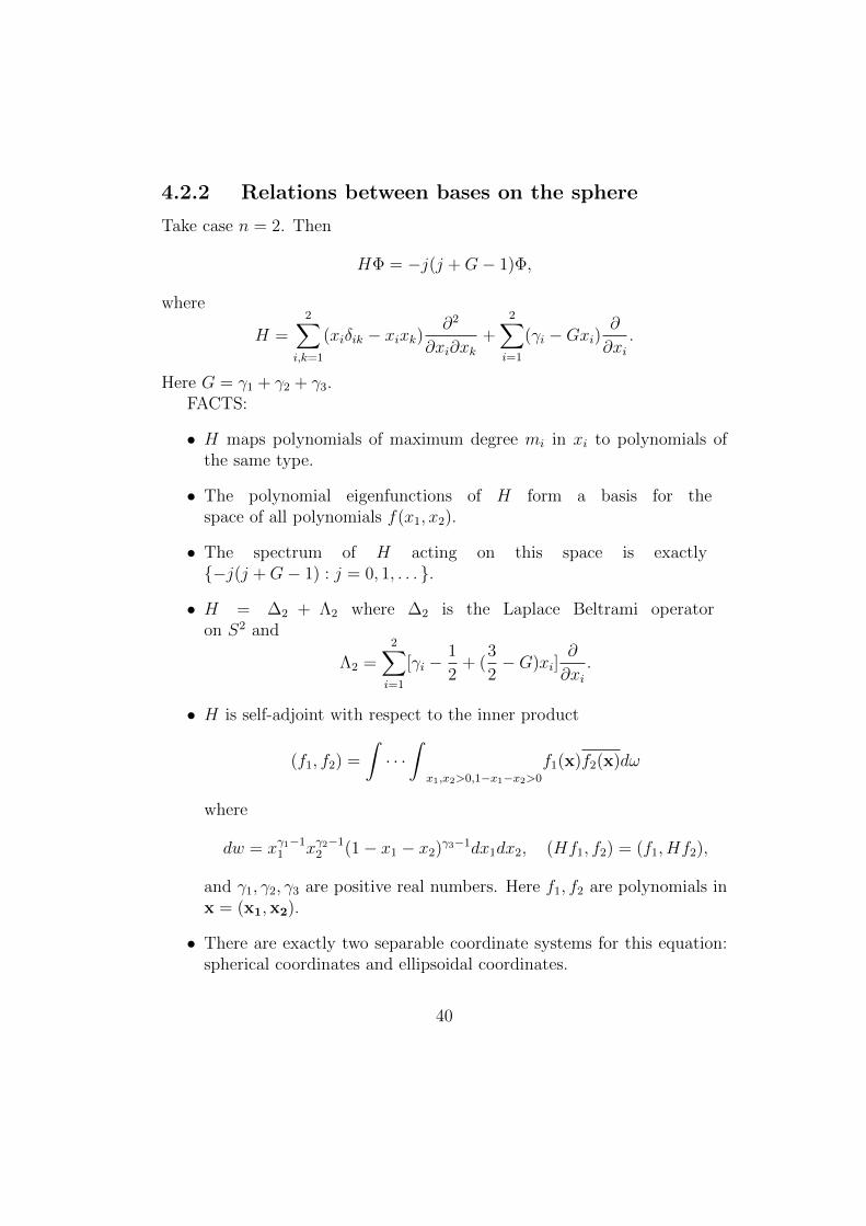
4.2.2 Relations between bases on the sphere

Take case n = 2. Then

HΦ = −j(j +G− 1)Φ,

where

H =2∑

i,k=1

(xiδik − xixk)∂2

∂xi∂xk+

2∑i=1

(γi −Gxi)∂

∂xi.

Here G = γ1 + γ2 + γ3.FACTS:

• H maps polynomials of maximum degree mi in xi to polynomials ofthe same type.

• The polynomial eigenfunctions of H form a basis for thespace of all polynomials f(x1, x2).

• The spectrum of H acting on this space is exactly{−j(j +G− 1) : j = 0, 1, . . . }.

• H = ∆2 + Λ2 where ∆2 is the Laplace Beltrami operatoron S2 and

Λ2 =2∑i=1

[γi −1

2+ (

3

2−G)xi]

∂

∂xi.

• H is self-adjoint with respect to the inner product

(f1, f2) =

∫· · ·∫

x1,x2>0,1−x1−x2>0

f1(x)f2(x)dω

where

dw = xγ1−11 xγ2−1

2 (1− x1 − x2)γ3−1dx1dx2, (Hf1, f2) = (f1, Hf2),

and γ1, γ2, γ3 are positive real numbers. Here f1, f2 are polynomials inx = (x1,x2).

• There are exactly two separable coordinate systems for this equation:spherical coordinates and ellipsoidal coordinates.

40

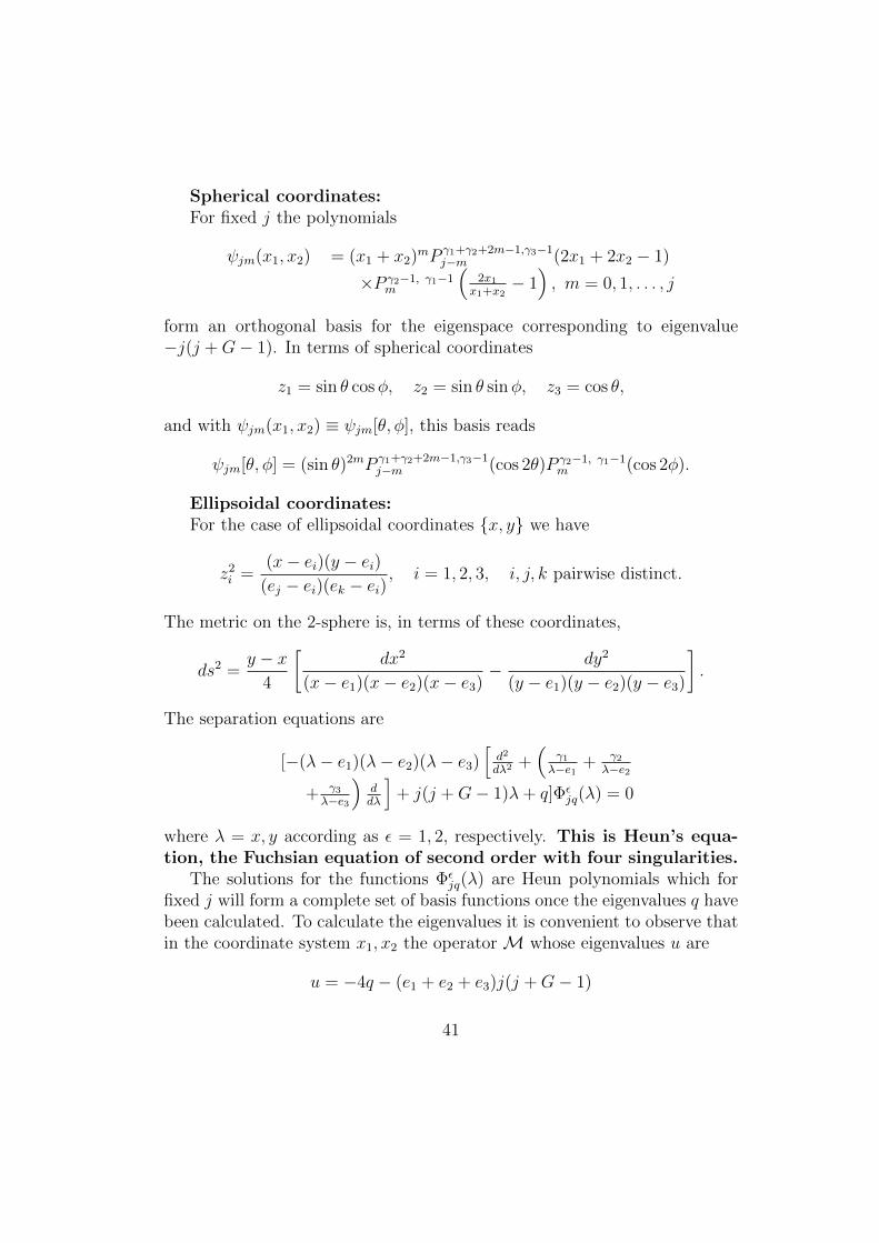
Spherical coordinates:For fixed j the polynomials

ψjm(x1, x2) = (x1 + x2)mP γ1+γ2+2m−1,γ3−1j−m (2x1 + 2x2 − 1)

×P γ2−1, γ1−1m

(2x1

x1+x2− 1), m = 0, 1, . . . , j

form an orthogonal basis for the eigenspace corresponding to eigenvalue−j(j +G− 1). In terms of spherical coordinates

z1 = sin θ cosφ, z2 = sin θ sinφ, z3 = cos θ,

and with ψjm(x1, x2) ≡ ψjm[θ, φ], this basis reads

ψjm[θ, φ] = (sin θ)2mP γ1+γ2+2m−1,γ3−1j−m (cos 2θ)P γ2−1, γ1−1

m (cos 2φ).

Ellipsoidal coordinates:For the case of ellipsoidal coordinates {x, y} we have

z2i =

(x− ei)(y − ei)(ej − ei)(ek − ei)

, i = 1, 2, 3, i, j, k pairwise distinct.

The metric on the 2-sphere is, in terms of these coordinates,

ds2 =y − x

4

[dx2

(x− e1)(x− e2)(x− e3)− dy2

(y − e1)(y − e2)(y − e3)

].

The separation equations are

[−(λ− e1)(λ− e2)(λ− e3)[d2

dλ2+(

γ1λ−e1 + γ2

λ−e2

+ γ3λ−e3

)ddλ

]+ j(j +G− 1)λ+ q]Φε

jq(λ) = 0

where λ = x, y according as ε = 1, 2, respectively. This is Heun’s equa-tion, the Fuchsian equation of second order with four singularities.

The solutions for the functions Φεjq(λ) are Heun polynomials which for

fixed j will form a complete set of basis functions once the eigenvalues q havebeen calculated. To calculate the eigenvalues it is convenient to observe thatin the coordinate system x1, x2 the operator M whose eigenvalues u are

u = −4q − (e1 + e2 + e3)j(j +G− 1)

41

is given by

M = (e1 + e2)S12 + (e2 + e3)S23 + (e1 + e3)S13

where the Sik are the symmetry operators. That is, M is the second or-der symmetry operator for the Laplacian ([M,∆] = 0) which correspondsto the separable coordinates x, y, and the Heun basis ψ = Φ1

jq(x)Φ2jq(y) is

characterized as the set of eigenfunctions Mψ = uψ.

Now we consider the problem of expanding the Heun basis Φ1jq(x)Φ2

jq(y)in terms of the Jacobi polynomial basis:

ψ = Φ1jq(x)Φ2

jq(y) =

j∑m=0

ξmψjm[θ, φ].

Three term recurrence relations for the expansion coefficients ξm can be de-duced by requiring that

Mψ = uψ.

To carry out the computation we need the action of the variouspieces Sik of M on the Jacobi bases ψjm[θ, φ]. We find

Mψjm[θ, φ] =+1∑r=−1

Xrψj,m+r[θ, φ]

where

X1(m, j) =4(e1 − e2)(γ1 + γ2 + γ3 +m+ j − 1)(γ3 −m+ j − 1)(m+ 1)

(γ1 + γ2 + 2m− 1)(γ1 + γ2 + 2m)(γ1+γ2+m−1),

X−1(m, j) =4(e1 − e2)(γ1 + γ2 +m+ j − 1)(−m+ j + 1)(γ2 − 1)(γ1 − 1)

(γ1 + γ2 + 2m− 1)(γ1 + γ2 + 2m− 2),

X0(m, j)−u =2(e1 − e2)[m2 +m(γ1 + γ2 − 1)− j2 − j(γ1 + γ2 + γ3 − 1)]

(γ1 + γ2 + 2m− 2)(γ1 + γ2 + 2m)(γ1+γ2−2)(γ1−γ2)

+4(e1 − e2)mγ3(γ1 − γ2)(m+ γ2)

(γ1 + γ2 + 2m− 2)(γ1 + γ2 + 2m)

+2(e1 + e2)[−m2 −m(γ1 + γ2 − 1) + j2 + j(γ1 + γ2 + γ3 − 1)]

+4e3[m2 +m(γ1 + γ2 − 1)] + 4q.

42

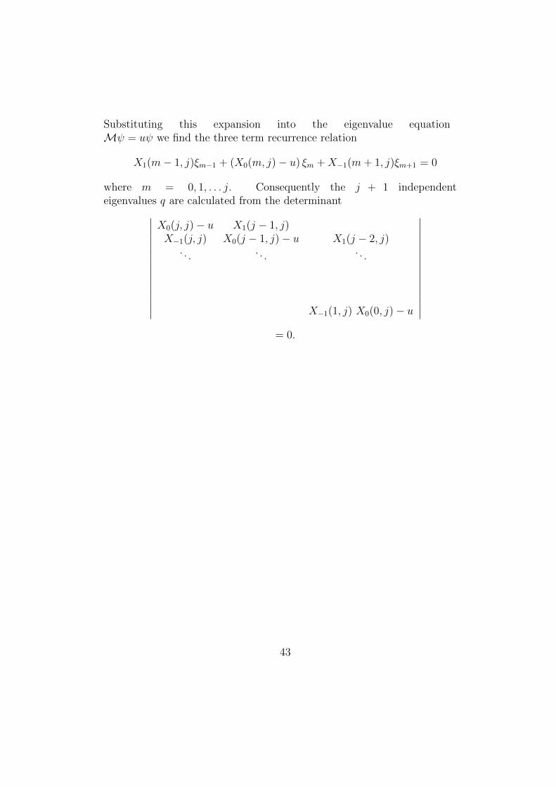
Substituting this expansion into the eigenvalue equationMψ = uψ we find the three term recurrence relation

X1(m− 1, j)ξm−1 + (X0(m, j)− u) ξm +X−1(m+ 1, j)ξm+1 = 0

where m = 0, 1, . . . j. Consequently the j + 1 independenteigenvalues q are calculated from the determinant∣∣∣∣∣∣∣∣∣∣∣∣∣∣∣

X0(j, j)− u X1(j − 1, j)X−1(j, j) X0(j − 1, j)− u X1(j − 2, j)

. . . . . . . . .

X−1(1, j) X0(0, j)− u

∣∣∣∣∣∣∣∣∣∣∣∣∣∣∣= 0.

43

Chapter 5

Clebsch-Gordan coefficientsand orthogonal polynomials

I will briefly indicate some relations between Clebsch-Gordan series for thedecomposition of tensor products of group representations and special func-tion theory. I will limit myself to a single example. The generalizations areobvious.

Example 3 SU(2).

SU(2) =

{A =

(α β−β α

): α, β ∈ C, |α|2 + |β|2 = 1

}.

L (SU(2)) = s`(2, R) =

{A =

(ix3 −x2 + ix1

x2 + ix1 −ix3

): xj ∈ R

}.

Basis for complexification of Lie algebra: L+, L−, L3

[L3, L±] = ±L±, [L+, L−] = 2L3.

L+ =

(0 −10 0

), L− =

(0 0−1 0

), L3 =

(12

00 1

2

).

This algebra is isomorphic to so(3).

Finite-dimensional representations

Tu(A)f(z) = (βz + β)2uf(αz − ββz + α

), 2u = 0, 1, 2, · · · ,

44

Orthonormal basis for representation space:

fm(z) =(−z)u+m√

(u−m)!(u+m)!, m = −u,−u+ 1, · · · , u− 1, u.

Action of Lie algebra:

L3fm = mfm, L±fm =√

(u±m+ 1)(u∓m)fm±1.

Note that the Casimir operator C = L+L− + L3L3 − L3 is a multiple of theidentity on the representation space: C = u(u+ 1)I.

Matrix elements: Tu(A)fm(z) =∑u

n=−u Unm(A)fn(z)Addition theorem for unitary matrix elements:

Unm(AB) =u∑

k=−u

Unk(A)Dkm(B), n,m = −u, · · · , u.

Decompose tensor product Tu ⊗ Tv (Clebsch-Gordan series):

Tu ⊗ Tv ≡u+v∑

w=|u−v|

⊕Tw.

Here,

L31f

(u)m = mf (u)

m , L±1 f(u)m =

√(u±m+ 1)(u∓m)f

(u)m±1.

L32f

(v)m = mf (v)

m , L±2 f(v)m =

√(v ±m+ 1)(v ∓m)f

(v)m±1.

Orthonormal basis for left-hand side: f(u)m ⊗ f (v)

n .Orthonormal basis for right-hand side:

h(w)k , w = |u− v|, · · · , u+ v, −w ≤ k ≤ w,

where

J3h(w)k = kh

(w)k , J±h

(w)k =

√(w ± k + 1)(w ∓ k)h

(w)k±1

andJ3 = L3

1, J+ = L+1 + L+

2 , J− = L−1 + L−2 .

45

The Clebsch-Gordan coefficients are the coefficients of the unitary matrixrelating these two bases:

h(w)k =

∑m,n

C(u,m; v, n|w, k)f (u)m ⊗ f (v)

n .

Relating the matrix elements of the group operators in the two bases, we findthe important identity

Uumm′(A)U v

nn′(A) =∑w,k,k′

C(u,m; v, n|w, k)C(u,m′; v, n′|w, k′)Uwkk′(A).

The C-G coefficients can be computed directly from our models, and are ex-pressible in terms of hypergeometric functions 3F2(1). They have importantsymmetries that follow from the group theory. These symmetries lead totransformation formulas for the 3F2(1).

To decompose this representation we compute the common eigenfunctionsof J3 and C = J+J− + J3J3 − J3. Clearly, eigenfunctions of J3 = L3

1 + L32

with eigenvalue s are just those linear combinations of the basis vectorsFαu+m = f

(u)m ⊗ f (v)

n where n = α −m. To be definite, suppose u ≤ v, α ≥ 0.Applying C to the ON set {Fα

k } we find a three term recurrence relation ofthe form

CFαk = akF

αk+1 + bkF

αk + ckFk−1

where ak, bk, ck are explicit. The operator C is self-adjoint with discreteeigenvalues w(w+ 1). If we introduce the spectral transform of this operatorso that C corresponds to multiplication by the transform variable x, then thisexpression takes the form of a three term recurrence relation for orthogonalpolynomials Fα

k (x) of order k in x. The functions Fαk (x) are, essentially, the

Clebsch-Gordan coefficients for this decomposition; the orthogonality andcompleteness relations for the polynomials are the unitarity conditions forthe C-G coefficients.

Insights along these lines lead to the Wilson polynomials, true generaliza-tions of the classical orthogonal polynomials, and finally to the Askey-Wilsonpolynomials. Indeed, the starting point for the Wilson polynomials is theRacah coefficients. These coefficients relate the basis vectors h

(s)k on the two

sides of the expression

(Tu ⊗ Tv)⊗ Tw ≡ Tu ⊗ (Tv ⊗ Tw).

46

The irreducible representation Ts may appear more than once so the Racahcoefficients are by no means trivial. They can be expressed as sums of prod-ucts of 4 C-G coefficients and then shown to be expressible in terms of hyper-geometric functions 4F3(1). They satisfy unitarity, symmetry and recurrencerelations, and one of those recurrence relations can be reinterpreted as a threeterm recurrence relation for a family of polynomials, the Racah polynomials.

47

Chapter 6

Harmonic analysis and latticesubgroups

We study two procedures for the analysis of time-dependent signals, locallyin both frequency and time. The first procedure, the “windowed Fouriertransform” is associated with the Heisenberg group while the second, the“wavelet transform” is associated with the affine group.

6.1 Harmonic analysis: windowed Fourier trans-

forms

Let g ∈ L2(R) with ||g|| = 1 and define the time-frequency translation of gby

g[x1,x2](t) = e2πitx2g(t+ x1) = T1[x1, x2, 0]g(t)

where T1 is the unitary irreducible representation

T1[x1, x2, x3]g(t) = e2πix3+2πitx2g(t+ x1)

of the Heisenberg group HR. Now suppose g is centered about the point(t0, ω0) in phase (time-frequency) space, i.e., suppose∫ ∞

−∞t|g(t)|2dt = t0,

∫ ∞−∞

ω|g(ω)|2dω = ω0

where g(ω) =∫∞−∞ g(t)e−2πiωtdt is the Fourier transform of g(t). Then∫ ∞

−∞t|g[x1,x2](t)|2dt = t0 − x1,

∫ ∞−∞

ω|g[x1,x2](t)|2dω = ω0 + x2

48

so g[x1,x2] is centered about (t0 − x1, ω0 + x2) in phase space. To analyze anarbitrary function f(t) in L2(R) we compute the inner product

F (x1, x2) = 〈f, g[x1,x2]〉 =

∫ ∞−∞

f(t)g[x1,x2](t)dt

with the idea that F (x1, x2) is sampling the behavior of f in a neighborhoodof the point (t0 − x1, ω0 + x2) in phase space. As x1, x2 range over all realnumbers the samples F (x1, x2) give us enough information to reconstructf(t).

However, the set of basis states g[x1,x2] is overcomplete: the coefficients〈f, g[x1,x2]〉 are not independent of one another, i.e., in general there is no f ∈L2(R) such that 〈f, g[x1,x2]〉 = F (x1, x2) for an arbitrary F ∈ L2(R2). Theg[x1,x2] are examples of coherent states, continuous overcomplete Hilbertspace bases which are of interest in quantum optics and quantum field theory,as well as gropup representation theory. Thus it isn’t necessary to computethe inner products 〈f, g[x1,x2]〉 = F (x1, x2) for every point in phase space.In the windowed Fourier approach one typically samples F at the latticepoints (x1, x2) = (ma, nb) where a, b are fixed positive numbers and m,nrange over the integers. Here, a, b and g(t) must be chosen so that the mapf −→ {F (ma, nb)} is one-to-one; then f can be recovered from the latticepoint values F (ma, nb). The study of when this can happen is the study ofWeyl-Heisenberg frames. It is particularly useful when g can be chosen suchthat g[ma,nb] is an ON basis for L2. This leads (in the case a = b) to the latticeHilbert space, the Weil-Brezin-Zak transform and important applications totheta functions.

6.2 Harmonic analysis: continuous wavelets

Here we work out the analog for the affine group of the Weyl-Heisenbergframe for the Heisenberg group. Let φ ∈ L2(R) with ||g|| = 1 and define theaffine translation of φ by

φ(a,b)(t) = a−1/2φ

(t+ b

a

)= L0[a, b]φ(t)

where a > 0 and L0 is the unitary representation

L0[a, b]φ(t) = a−1/2φ

(t+ b

a

)49

of the affine group.Can assume that

∫∞−∞ t|φ(t)|2dt = 0. Let k =

∫∞0y|φ(y)|2dy. Then φ is

centered about the origin in position space and about k in momentum space.It follows that∫ ∞

−∞t|φ(a,b)(t)|2dt = −b,

∫ ∞0

y|φ(a,b)(y)|2dy = a−1k.

To define a lattice in the affine group space we choose two nonzero realnumbers a0, b0 > 0 with a0 6= 1. Then the lattice points are a = am0 , b =nb0a

m0 , m,n = 0,±1, · · · , so

φmn(t) = φ(am0 ,nb0am0 )(t) = a

−m/20 φ(a−m0 t+ nb0).

Thus φmn is centered about −nb0am0 in position space and about a−m0 k in

momentum space. (Note that this behavior is very different from the behaviorof the Heisenberg translates g[ma,nb]. In the Heisenberg case the support of gin either position or momentum space is the same as the support of g[ma,nb]. Inthe affine case the sampling of position-momentum space is on a logarithmicscale. There is the possibility, through the choice of m and n, of sampling insmaller and smaller neighborhoods of a fixed point in position space.)

The affine translates φ(a,b) are called wavelets and the function φ is afather wavelet. The map T : f −→

∫f(t)φmn(t)dt is the continuous

wavelet transformAgain the continuous wavelet transform is overcomplete. The question

is whether we can find a subgroup lattice and a function φ for which thefunctions

φmn(t) = φ(am0 ,nb0am0 )(t) = a

−m/20 φ(a−m0 t+ nb0)

generate an ON basis. We will choose a0 = 1/2, b0 = 1 and find conditionssuch that the functions

φmn = 2m/2φ(2mt+ n), m, n = 0,±1,±2, · · ·

span L2. In particular we will require that the set φ0n(t) = φ(t + n) beorthonormal.

50

6.3 Harmonic analysis: discrete wavelets and

the multiresolution structure

From the discussion of the last section, we want to find a scaling function(or father wavelet) φ such that the functions φmn(t) = 2m/2φ(2mt + n) willgenerate an ON basis for L2. In particular we require that the set φ0n(t) =φ(t + n) be orthonormal. Then for each fixed m we will have that {φmn} isON in n.

EXAMPLE: The Haar scaling function

φ(t) =

{1 0 ≤ t < 1.0 otherwise

Here the set {φ(t + n) = φ0n : n = 0,±1, · · · } is ON. Let Vm be the spaceof piecewise constant functions in L2(R) with possible discontinuities only atthe gridpoints tk = k

2mj , k = 0,±1,±2 · · · . Note that

1. {φmn(t) : n = 0,±1, · · · } is an ON basis for Vm.

2. Vm ⊂ Vm+1

3. ∪mVm = L2(R)

4. φ(t) = φ(2t) + φ(2t− 1).

This example leads naturally to the concept of a multiresolution structureon L2.

Definition 9 Let {Vj : j = · · · ,−1, 0, 1, · · · } be a sequence of subspaces ofL2[−∞,∞] and φ ∈ V0. This is a multiresolution analysis for L2[−∞,∞]provided the following conditions hold:

1. The subspaces are nested: Vj ⊂ Vj+1.

2. The union of the subspaces generates L2 : ∪∞j=−∞Vj = L2[−∞,∞].(Thus, each f ∈ L2 can be obtained a a limit of a Cauchy sequence{sn : n = 1, 2, · · · } such that each sn ∈ Vjn for some integer jn.)

3. Separation: ∩∞j=−∞Vj = {0}, the subspace containing only the zerofunction. (Thus only the zero function is common to all subspaces Vj.)

51

4. Scale invariance: f(t) ∈ Vj ⇐⇒ f(2t) ∈ Vj+1.

5. Shift invariance of V0: f(t) ∈ V0 ⇐⇒ f(t− k) ∈ V0 for all integers k.

6. ON basis: The set {φ(t− k) : k = 0,±1, · · · } is an ON basis for V0.

Here, the function φ(t) is called the scaling function (or the father wavelet).

Of special interest is a multiresolution analysis with a scaling functionφ(t) on the real line that has compact support. The functions φ(t + k) willform an ON basis for V0 as k runs over the integers, and their integrals withany polynomial in t will be finite.

• Can we find continuous scaling functions with compact sup-port?

Given φ(t) we can define the functions

φjk(t) = 2j2φ(2jt− k), k = 0,±1,±2, · · ·

and for fixed integer j they will form an ON basis for Vj. Since V0 ⊂ V1 itfollows that φ ∈ V1 and φ can be expanded in terms of the ON basis {φ1k}for V1. Thus we have the dilation equation

φ(t) =√

2∑k

c(k)φ(2t− k),

or, equivalently,

φ(t) = 2N∑k=0

h(k)φ(2t− k)

where h(k) = 1√2c(k). Since the φjk form an ON set, the coefficient vector c

must be a unit vector in `2, ∑k

|c(k)|2 = 1.

Since φ(t) ⊥ φ(t−m) for all nonzerom, the vector c satisfies the orthogonalityrelation:

(φ00, φ0m) =∑k

c(k)c(k − 2m) = δ0m.

52

Lemma 1 If the scaling function is normalised so that∫ ∞−∞

φ(t)dt = 1,

then∑N

k=0 c(k) =√

2.

We can introduce the orthogonal complement Wj of Vj in Vj+1.

Vj+1 = Vj ⊕Wj.

We start by trying to find an ON basis for the wavelet space W0. Associatedwith the father wavelet φ(t) there must be a mother wavelet w(t) ∈ W0, withnorm 1, and satisfying the wavelet equation

w(t) =√

2∑k

d(k)φ(2t− k),

and such that w is orthogonal to all translations φ(t−k) of the father wavelet.We further require that w is orthogonal to integer translations of itself. Sincethe φjk form an ON set, the coefficient vector d must be a unit vector in `2,∑

k

|d(k)|2 = 1.

Moreover since w(t) ⊥ φ(t − m) for all m, the vector d satisfies so-calleddouble-shift orthogonality with c:

(w, φ0m) =∑k

c(k)d(k − 2m) = 0. (6.1)

The requirement that w(t) ⊥ w(t−m) for nonzero integer m leads to double-shift orthogonality of d to itself:

(w(t), w(t−m)) =∑k

d(k)d(k − 2m) = δ0m. (6.2)

However, if the unit coefficient vector c is double-shift orthogonal then thecoefficient vector d defined by

d(n) = (−1)nc(N − n). (6.3)

automatically satisfies the conditions (6.1) and (6.2).

53

Theorem 3

L2[−∞,∞] = Vj ⊕∞∑k=j

Wk = Vj ⊕Wj ⊕Wj+1 ⊕ · · · ,

so that each f(t) ∈ L2[−∞,∞] can be written uniquely in the form

f = fj +∞∑k=j

wk, wk ∈ Wk, fj ∈ Vj. (6.4)

To find compact support wavelets must find solutions c(k) of the orthogonal-ity relations above, nonzero for a finite range k = 0, 1, · · · , N . Then given asolution c(k) must solve the dilation equation

φ(t) =√

2∑k

c(k)φ(2t− k). (6.5)

to get φ(t). Can show that the support of φ(t) must be contained in theinterval [0, N).

One way to try to determine a scaling function φ(t) from the impulseresponse vector c is to iterate the dilation equation. That is, we start withan initial guess φ(0)(t), the Haar scaling function on [0, 1), and then iterate

φ(i+1)(t) =√

2N∑k=0

c(k)φ(i)(2t− k) (6.6)

This is called the cascade algorithm.The frequency domain formulation of the dilation equation is :

φ(ω) =

(∑k

h(k)e−iωk/2

)φ(ω

2)

where c(k) =√

2h(k). Thus

φ(ω) = H(ω

2)φ(

ω

2).

where

H(ω) =N∑k=0

h(k)e−iωk

54

Iteration yields the explicit infinite product formula: φ(ω):

φ(ω) = Π∞j=1H(ω

2j). (6.7)

φ(t) IS A SPECIAL FUNCTION

• Daubechies has found a solution c(k) and the associated scaling func-tion for each N = 1, 3, 5, · · · . (There are no solutions for even N .)Denote these solutions by DM = DN+1 = D2p. D2 is just the Haarfunction. Daubechies finds the unique solutions for which the Fouriertransform of the impulse response vector C(ω) has a zero of order p atω = π, where 2p = N + 1. (At each N this is the maximal possiblevalue for p.)

• Can compute the values of φ(t) exactly at all dyadic points t =∑

njn2n

,jn = ±1.

•∑

k φ( k2j

) = 2j for j = 0, 1, 2, · · · .

• Can find explicit expressions∑k

y`kφ(t+ k) = t`, ` = 0, 1, · · · , p− 1,

so polynomials in t of order ≤ p − 1 can be expressed in V0 with noerror.

• The support of φ(t) is contained in [0, N), and φ(t) is orthogonal to allinteger translates of itself. The wavelets {wmn} form an ON basis forL2.

• B-splines fit into this multiresolution framework, though more natu-rally with biorthogonal wavelets.

• There are matrices

T = (↓ 2)2HHtr

= MHtr.

associated with each of the Daubechies solutions whose eigenvalue stru-ture determines the convergence properties of the wavelet expansions.These matrices have beautiful eigenvalue structures.

55

• There is a smoothness theory for Daubechies DM . Recall M = N+1 =2p. The smoothness grows with p. For p = 1 (Haar) the scalingfunction is piecewise continuous. For p = 2, (D4) the scaling functionis continuous but not differentiable. For p ≥ 3 we have s = 1 (onederivative). For p = 5, 6, 7, 8 we have s = 2. For p = 9, 10 we haves = 3. Asymptotically s grows as 0.2075p+ constant.

• The constants c are explicit for N = 1, 3. For N = 5, 7, · · · they mustbe computed numerically.

Example 4 The nonzero Daubechies filter coefficients for D4 (N = 3) are4√

2c(k) = 1 +√

3, 3 +√

3, 3 −√

3, 1 −√

3. With the normalization φ(0) +φ(1) + φ(2) = 1 we have, uniquely,

φ(0) = 0, φ(1) =1

2(1 +

√3) φ(2) =

1

2(1−

√3).

From these three values the values of φ(t) at any dyadic point can be computedexplicitly.

Wavelets are extremely useful in signal analysis, data compression (in-cluding image compression), edge detection, noise removal, etc.

56

Chapter 7

Significant researchopportunities and challenges

• The study of many-variable hypergeometric functions via the canonicalequations/ Gel’fand approach. q-analogs.

• Study of the analogs of windowed Fourier transforms and wavelet trans-forms in higher dimensions.

• Study of the relationship between Clebsch-Gordon coefficients for semi-simple Lie algebras and multivariable orthogonal polynomials. q-analogs.

• The “magic” potentials discussed earlier are examples of superinte-grable systems, Hamiltonian systems in N variables that admit 2N −1independent second order constants of the motion. These are integrablesystems with the maximum possible symmetry and are intimately re-lated to special function theory. The complete classification and anal-ysis of these systems is an important task.

• In contrast to the theory of orthogonal variable separation for constantcurvature spaces, classification of nonorthogonal separable systems isnot well understood.

• Study of the special functions arising as solutions of the spin equationsof general relativity. Teukolsky functions.

57