The Leverage of Demographic Dynamics on Carbon Dioxide ... · PDF fileThe Leverage of...

The Leverage of Demographic Dynamics on CarbonDioxide Emissions: Does Age Structure Matter?

Emilio Zagheni

Published online: 17 February 2011# The Author(s) 2011. This article is published with open access at Springerlink.com

Abstract This article provides a methodological contribution to the study of the effectof changes in population age structure on carbon dioxide (CO2) emissions. First, Ipropose a generalization of the IPAT equation to a multisector economy with an age-structured population and discuss the insights that can be obtained in the context ofstable population theory. Second, I suggest a statistical model of householdconsumption as a function of household size and age structure to quantitativelyevaluate the extent of economies of scale in consumption of energy-intensive goods,and to estimate age-specific profiles of consumption of energy-intensive goods andof CO2 emissions. Third, I offer an illustration of the methodologies using data forthe United States. The analysis shows that per-capita CO2 emissions increase withage until the individual is in his or her 60s, and then emissions tend to decrease.Holding everything else constant, the expected change in U.S. population agedistribution during the next four decades is likely to have a small, but noticeable,positive impact on CO2 emissions.

Keywords CO2 emissions . Climate change . IPAT. Input-output models . Populationage structure

Introduction

Demographic trends and changes in economic production are major factors drivinganthropogenic greenhouse gas emissions (e.g., O’Neill et al. 2001), which, in turn,are most likely responsible for the observed increase in average global temperaturesover the last few decades (IPCC 2007). Although several demographic quantities arepotentially important determinants of greenhouse gas emissions (e.g., O’Neill andChen 2002; Schipper 1996), most models used to develop emissions scenarios

Demography (2011) 48:371–399DOI 10.1007/s13524-010-0004-1

E. Zagheni (*)Department of Demography, University of California, Berkeley,2232 Piedmont Avenue, Berkeley, CA 94720-2120, USAe-mail: [email protected]

explicitly consider only population size or, in a few cases, some aggregate measuresof age structure (O’Neill 2005).

This article contributes to the study of the effect of changing population agestructure on emissions of carbon dioxide (CO2), the gas that accounts for most of theanthropogenic-driven greenhouse effect. I offer new methodological perspectivesthat bridge the gap between the literatures on IPAT-based approaches (e.g., Chertow2001) and environmental input-output modeling (e.g., Hendrickson et al. 2006). Ipropose a model that can be interpreted as a generalization of the IPAT equation to amultisector economy with an age-structured population. The model provides aunified interpretation of previous IPAT-based studies of the effect of population agecomposition and economic structure on CO2 emissions. It can also be seen as a staticversion of the general equilibrium model, with multiple dynasties of households, assuggested by Dalton et al. (2008). A major contribution of the article is thedevelopment of methods to estimate the life cycle profile of CO2 emissions forindividuals. The methodologies that I propose are applied to data for the UnitedStates, showing that the expected change in population age structure over the nextfour decades is likely to have a positive, but rather small, impact on CO2 emissions,holding everything else constant.

Background

Two main approaches have been proposed to study the role played by population agestructure in shaping the level of greenhouse gas emissions. The first approachoriginates from the conceptual framework provided by the so-called IPAT equation(Commoner 1972; Ehrlich and Holdren 1971, 1972). The second approach mostlyrelies on integrated energy-economic growth models, such as the Population-Environment-Technology model, that are calibrated with household demographicprojections, input-output economic tables, and estimates of consumption expenditures,savings, labor supply, etc. (e.g., Dalton et al. 2008).

The IPAT equation is an accounting identity that was proposed in the early 1970sto conceptualize the multiplicative role of population size on measures ofenvironmental disruption (Commoner 1972; Ehrlich and Holdren 1971, 1972). Theidentity decomposes environmental impact (I) into the product of population size(P), affluence (A), and technology (T):

I ¼ P � A� T ; ð1Þwhere affluence is operationalized as per-capita income (Y/P), and technology isexpressed as environmental impact per unit of economic production (I/Y).

The IPAT equation was suggested in a period when environmental concernsfocused on the ability of the environment to absorb pollutants that are by-products ofmodern technology (e.g., pesticides, asbestos, radioactive waste, petrochemicals,household waste) (Pebley 1998; Ruttan 1993). In the early 1990s, environmentalconcerns shifted toward changes occurring on a global scale, such as climate change.In this new context, the IPAT conceptual framework has strongly influenced researchcarried out by demographers on the impact of demographic factors on greenhousegas emissions (Pebley 1998).

372 E. Zagheni

Dietz and Rosa (1994) made the IPAT equation operational for statistical analysis.Their formulation, known as STIRPAT (Stochastic Impacts by Regression onPopulation, Affluence and Technology), has been extensively used to evaluate therole of demographic factors in the explanation of CO2 emissions. Population size hasbeen the main demographic variable under analysis. Dietz and colleagues estimateda unitary elasticity of CO2 emissions with respect to population size, using a cross-national data sample (Dietz and Rosa 1997; Rosa et al. 2004; York et al. 2003).They thus empirically supported the underlying assumption of the IPAT equation ofunitary elasticity of I with respect to P. On the other hand, Shi (2003) obtained ahigher estimate. Based on a panel data set for 93 countries for the period 1975–1996, Shi estimated that a 1% increase in population size raises emissions onaverage by 1.4%.

The role of several demographic variables on CO2 emissions has beenevaluated within the context of IPAT-based models. For instance, York et al.(2003) showed that urbanization is positively correlated with CO2 emissions. Mostimportantly for the purposes of this study, the IPAT framework has stimulatedsome investigation of the effect of changing age structure on CO2 emissions. Dietzand Rosa (1994) suggested that countries with a higher proportion of working-agepopulation consume more energy and resources and thus produce more emissions.MacKellar et al. (1995) used households, instead of individuals, as the unit ofanalysis for their IPAT-based model and showed that population aging may have alarge, positive impact on CO2 emissions. As a matter of fact, population aging ispartly responsible for the observed increase in number of households in the moredeveloped regions of the world over the last several decades. The growth inhousehold numbers in more developed regions of the world is projected to besubstantially larger than population growth, leading to higher levels of CO2

emissions than accounted for by models that do not consider changes in agestructure and behavioral determinants of household formation and dissolution(Mackellar et al. 1995). Shi (2003) found a positive association betweenpercentage of population in working age and CO2 emissions. Fan et al. (2006)concluded that the proportion of the population between ages 15 and 64 has anegative impact on CO2 emissions for countries with a high income level, whereasit has a positive impact for countries at other income levels. The effects of agestructure are mediated by the labor force’s productions and individual behaviors.O’Neill and Chen (2002) discussed the limitations of IPAT decompositions andprovided a standardization exercise for the United States, showing that the increasein the fraction of the population living with a householder older than 65 years willincrease residential energy use and decrease transportation energy use, withconsequences for CO2 emissions.

In the IPAT literature, there has been some discussion about the differentialimpact on CO2 emissions of population dynamics associated with differenteconomic structures. For instance, Shi (2003) showed that the elasticity of CO2

emissions with respect to population size depends on the level of income of thecountry. The lowest elasticity is estimated for high-income countries (0.83%) andthe highest is estimated for lower-middle-income countries (1.97%). This result isconsistent with the observation that the structure of the economy is important forthe explanation of levels of emissions (York et al. 2003) and that the impact of

The Leverage of Demographic Dynamics on Carbon Dioxide Emissions 373

population is different at different levels of development (Fan et al. 2006). In IPAT-based models, it has thus been suggested to consider the relative importance ofmanufacture production versus services, to capture the difference in the economicstructure of each country (Shi 2003).

More detailed analyses of the role of the economic structure in the explanation ofenvironmental outcomes have been done using input-output economic models,which date back to the pioneering work of Leontief (e.g. 1936, 1953, 1970, 1986). Inthe context of demographic analysis of environmental impact, relevant contributionsappeared in the 1970s, when the U.S. Commission on Population Growth and theAmerican Future asked Resources for the Future, a research organization, toundertake a project to identify the principal resource and environmental consequen-ces of future population growth in the United States. The project was an importantattempt to assess the environmental consequences of demographic, economic, andtechnological dynamics using input-output economic tables (Herzog and Ridker1972; Ridker 1972).

The application of input-output economic analysis to environmental studies hasgrown with the goal of providing information about the environmental impacts ofindustrial production processes. This has typically been done by analyzing resourceuse and flows of industrial products, consumer products, and wastes. Duchin hasworked extensively on the theory and methods that relate changes in technology,lifestyles, and the environment (e.g., Duchin 1998; Duchin and Lange 1994).Among other work, she has discussed the challenge of describing concretetechnological and lifestyle alternatives that work best to tackle environmentalproblems. She suggested classifying household types in different societies accordingto common patterns of work, leisure, consumption, attitudes, and values, and toevaluate how activities are carried out in different societies, their outcomes, and thebest alternatives to obtain a specific result (Duchin 1996).

The past two decades have seen increased attention to the role played byconsumers and their lifestyles on environmental outcomes (Bin and Dowlatabadi2005). Schipper and colleagues linked energy use to consumers’ activities, timeuse, and demographic variables. They estimated that about half of total energy use isinfluenced by personal transportation, personal services, and home energy use (Schipper1996; Schipper et al. 1989). Reinders et al. (2003) extended studies of energyrequirements of households in the Netherlands (e.g., Vringer and Blok 1995) to severalEuropean countries. They used household budget data to evaluate the relationshipbetween household expenditures and energy use, and they found that the share ofdirect energy in the total energy requirement ranges from 34% to 64% in the countriesconsidered. Lenzen (1998) used an input-output approach to evaluate energy use inAustralia. He concluded that most greenhouse gas emissions are ultimately attributableto household purchases of goods and services and that the increase in emissions isstrongly correlated with income growth. Pachauri and Spreng (2002) proposed a studyof household energy requirements in India based on input-output tables and found thatthe main drivers of energy requirements are per-capita expenditures, population trends,and energy intensity in the food and agricultural sectors. Hertwich (2005) reviewed theenvironmental impact of household consumption in the context of integrated input-output models and life cycle analysis of products. He showed that in more-developedcountries, household consumption is the most important final demand category in

374 E. Zagheni

terms of energy use and CO2 emissions. In developing countries, exports are moreimportant if there are a lot of heavily export-oriented industries. Peters and Hertwich(2008) discussed the advantages of a consumption-based approach versus aproduction-based approach in constructing greenhouse gas inventories that accountfor international trade. Based on a detailed study for Norway, they also showed that theenvironmental impacts of consumers may be underestimated if emissions embodied inimports are not taken into account (Peters and Hertwich 2006). Tukker and Jansen(2006) provided a review of studies of environmental impact of products. The mainidea behind these studies is that consumption of households and governments drivesthe environmental effects of economic activities, both directly and indirectly, throughthe impacts of production, use, and waste management of economic goods. Across allstudies considered for European countries, expenditures on housing (including heatingand electricity use), transportation, and food account for most emissions of CO2. In thecase of the United States, Bin and Dowlatabadi (2005) estimated that CO2 emissionsrelated to direct influences (emissions that occur while the product or service is in use,e.g., personal travel) are about 70% of those related to indirect influences (emissionsthat occur during the production and delivery of a product or service, e.g.,transportation operation, food). Their results are partly based on the use of theEnvironmental Input-Output Life Cycle Analysis (EIO-LCA) model developed atCarnegie Mellon University (Hendrickson et al. 2006). The main implication of thesestudies is that both direct and indirect energy use have to be considered in theevaluation of the role played by consumers’ lifestyles on CO2 emissions.

The literature that relies on economic input-output tables to analyze the impactof consumption on energy use and CO2 emissions is extensive. However, littleattention has been given to the role of specific demographic factors, such aspopulation age structure. Dalton et al. (2008) offer a notable exception. Theyincorporated household age structure into a dynamic energy-economic growthmodel and estimated that population aging may reduce long-term CO2 emissions inthe United States.

In this article, I integrate the approaches developed in the two areas of IPAT-based modeling and environmental input-output analysis to evaluate the effect ofchanging population-age structure on CO2 emissions in the United States.Methodologically, I first present a generalization of the IPAT equation to amultisector economy with an age-structured population, and I discuss the insightsobtained in the context of stable population theory (e.g., Keyfitz and Caswell2005). Second, I propose a statistical framework to calibrate the theoretical model.In particular, I suggest a model of household consumption as a function ofhousehold size and age structure. The model is used to evaluate the extent ofeconomies of scale in consumption of energy-intensive goods and to estimate age-specific consumption profiles.

I look at age profiles of consumption from an individual, rather than a household,perspective. There are advantages and disadvantages to using either households orindividuals as the unit of analysis. For instance, some household characteristics havebeen identified as key determinants of residential energy demand (e.g., O’Neill andChen 2002; Schipper 1996; Schipper et al. 1989). In addition, household size mayhave important consequences on per-capita energy use because of the existence ofeconomies of scale at the household level (e.g., Vringer and Blok 1995). On the


other hand, within the framework that I propose, the choice of the individual makesit simpler to evaluate the effects of changes in age structure. It also potentially makesit easier to incorporate the work that I propose into the economic demographyliterature that explores the macroeconomic consequences of population aging, andwhose unit of analysis is the individual (e.g., Lee 1994, 2000; Lee et al. 2006).

Empirically, I offer an illustration of the methodologies that I propose using datafor the United States. I estimate the extent of economies of scale in consumptionfrom cohabitation, for a set of energy-intensive goods, and I derive age-specificconsumption profiles for the same goods. These results are then used to estimate anage-specific profile of emissions. They are also used as inputs for the theoreticalmodel in order to evaluate expected variations in CO2 emissions associated withchanges in population growth and age structure.

The Theoretical Model

This section is dedicated to the formal discussion of the conceptual scheme that Ipropose to use to analyze the impact of demographic dynamics on CO2 emissions.

First, I offer a generalization of the IPAT equation to a multisector economy withan age-structured population. The model is intended to capture the environmentalconsequences of changes in population age structure, mediated by levels of per-capita consumption, existing technology, and interrelationships between sectors ofthe economy.

Second, I formally analyze the effect of changes in mortality and fertility rates onthe growth rate and age structure of a stable population, and the relatedconsequences on CO2 emissions. I show the analogies between the classical IPATapproach and its generalization, and I discuss the additional insights that can begleaned from the latter.

A Generalization of the IPAT Equation

I propose a theoretical model that can be interpreted as a generalization of the IPATequation to a multisector economy with an age-structured population. First, I providea formal description of an input-output model for environmental analysis, using thenotation of Hendrickson et al. (2006). Then, I introduce a demographic component(e.g., population age structure) to the model, and I discuss its role with reference toIPAT-based modeling.

Consider an economy with m sectors, indexed by i. The total monetary output forsector i, yi, is written as

yi ¼ zi1 þ zi2 þ :::þ zim þ di; ð2Þwhere zij is the monetary flow of goods from sector i to sector j, and di is the finaldemand for the good i. The model is typically rewritten to represent the flowsbetween sectors as a percentage of sectoral output. Thus, if I write

qij ¼ zijyj;

376 E. Zagheni

the model is expressed as

yi ¼ qi1y1 þ qi2y2 þ . . .þ qimym þ di ð3Þ

or, equivalently,

�qi1y1 � qi2y2 � � � � þ ð1� qiiÞyi � � � � � qimym ¼ di: ð4Þ

By letting Q be the m × m matrix containing all the coefficients qj, Y be the m × 1vector containing all the output yi terms, and D be the m × 1 vector of final demandsdi, the model is written in a more compact form as follows:

I�Q½ �Y ¼ D: ð5Þ

This way, given the vector of final demands and the matrix of coefficients Q, thevector of outputs by sector is obtained as

Y ¼ I�Q½ ��1D: ð6ÞHendrickson et al. (2006) used this model to evaluate human environmental

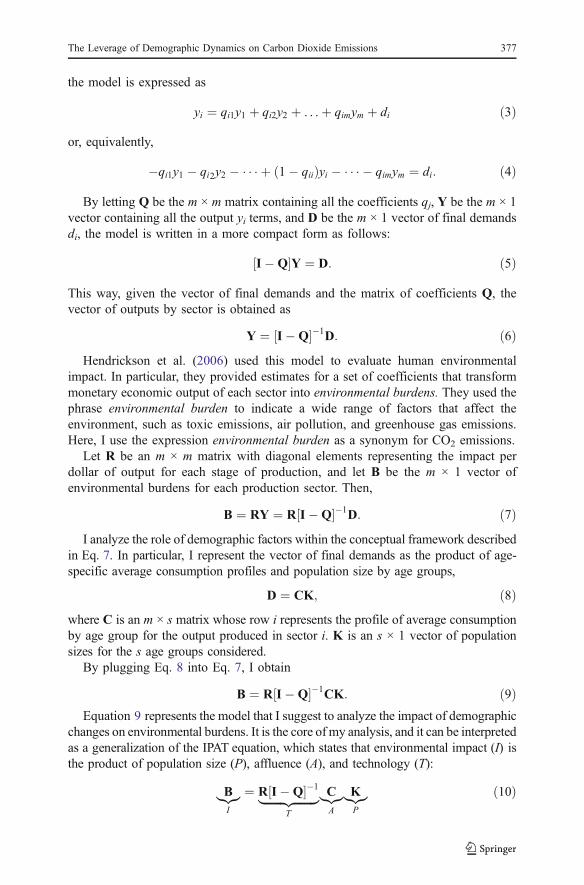
impact. In particular, they provided estimates for a set of coefficients that transformmonetary economic output of each sector into environmental burdens. They used thephrase environmental burden to indicate a wide range of factors that affect theenvironment, such as toxic emissions, air pollution, and greenhouse gas emissions.Here, I use the expression environmental burden as a synonym for CO2 emissions.

Let R be an m × m matrix with diagonal elements representing the impact perdollar of output for each stage of production, and let B be the m × 1 vector ofenvironmental burdens for each production sector. Then,

B ¼ RY ¼ R I�Q½ ��1D: ð7ÞI analyze the role of demographic factors within the conceptual framework described

in Eq. 7. In particular, I represent the vector of final demands as the product of age-specific average consumption profiles and population size by age groups,

D ¼ CK; ð8Þwhere C is an m × s matrix whose row i represents the profile of average consumptionby age group for the output produced in sector i. K is an s × 1 vector of populationsizes for the s age groups considered.

By plugging Eq. 8 into Eq. 7, I obtain

B ¼ R I�Q½ ��1CK: ð9ÞEquation 9 represents the model that I suggest to analyze the impact of demographic

changes on environmental burdens. It is the core of my analysis, and it can be interpretedas a generalization of the IPAT equation, which states that environmental impact (I) isthe product of population size (P), affluence (A), and technology (T):

B|{z}I

¼ R I�Q½ ��1|fflfflfflfflfflfflffl{zfflfflfflfflfflfflffl}T

C|{z}A

K|{z}P

ð10Þ


In the conceptual framework that I suggest, the vector B of environmentalburdens corresponds to the scalar I in the IPAT equation. K has the role of P, thedemographic factor. C represents the level of age-specific per-capita consumptionand can be interpreted as the level of affluence, or A in the IPAT terminology.Finally, R I�Q½ ��1 is a product of terms that is intended to give a syntheticrepresentation of the technology in use, the structure of the economy, the level ofenergy efficiency, the carbon intensity of the energy supply (i.e., types of fuels usedin production or consumption), and so on. It has a role analogous to the one of the Tterm in the IPAT equation because it translates monetary value into units ofenvironmental impact (e.g., metric tons of CO2 emissions).

The model that I propose is a generalization of the IPAT equation to a multisectoreconomy with an age-structured population. When we consider an economy with onlyone sector and ignore population age structure, the model reduces to the one depicted bythe IPAT equation. In addition, the model differentiates consumption according to thesectors of the economy to which we can impute the production of final goods and thusgeneralizes the study ofWaggoner and Ausubel (2002), who reconceptualized the IPATidentity in order to separate the leverage of “workers” from the one of “consumers.”

This article focuses on the role of population age structure, but the model representedin Eq. 10 is very general and can account for other types of demographic heterogeneity,such as urban-rural differences. This could be done by having the K column vectorrepresent age-specific population sizes by urban and rural residency, one after the other.Then the component C will be a block matrix with age-specific profiles of consumptionby residency. The term CK will give a vector of age-specific final demand forconsumption goods by residency. This vector, when multiplied by an appropriate matrixof indicator variables, will generate a vector of overall demands of consumption goods.

The Leverage of a Change in Mortality and Fertility

In order to obtain insights on the effect of changes in mortality and fertility rates onCO2 emissions, I consider the generalization of the IPAT equation within theframework of stable population theory (e.g., Keyfitz and Caswell 2005) and theSolow model of economic growth (Solow 1956). First, I discuss the insights that canbe uncovered in the context of a traditional IPAT-based approach. Then, I extend theanalysis to the generalization that I propose, and I discuss the additional insights.

The IPATapproachwas originally introducedwith the intention of refusing the notionthat demography is only a minor contributor to environmental crises and with the goal ofshowing that population size and growth are relevant quantities in the explanation ofenvironmental outcomes (Ehrlich and Holdren 1971). One of the major points in theIPAT literature is that population size (P) has a multiplicative role on environmentalimpacts (I). Several representations of the original IPAT identity have been suggestedin the literature in order to make the approach operative for statistical analysis (e.g.,Chertow 2001; Dietz and Rosa 1994, 1997). One way to look at IPAT-based models isto rearrange the terms in order to express the growth rate of CO2 emissions in terms ofpopulation and income growth rates (e.g., Preston 1996; Zagheni and Billari 2007):

I�

I¼ f

P�

Pþϕ

Y�

Y; ð11Þ

378 E. Zagheni

where I�, P�, and Y

�are, respectively, the first derivatives of CO2 emissions, population

size, and income with respect to time. ϕ and φ are parameters.Assuming that the economy can be represented with a neoclassic model of

economic growth, such as the Solow model, then in steady-state, the output growth

rate Y�t=Yt

� �is determined by the rate of technological progress (g), the growth rate

of the labor force (r), and a factor controlling for the extent of diminishing marginalreturns to capital (α):

Y�

Y¼ g

1� αþ r: ð12Þ

By plugging Eq. 12 into Eq. 11 and considering the case of a stable population,I obtain

I�

I¼ ð f þϕÞr þϕ

g

1� α: ð13Þ

Since I am considering a population with stable age structure, the population andlabor force growth rate, r, can be linearly approximated to

r � lnðNRRÞaf

; ð14Þ

where NRR is the net reproduction ratio and af is the mean age at childbearing.By plugging Eq. 14 into Eq. 13, and expressing the NRR in terms of its

components, the growth rate of CO2 emissions becomes

I�

I� ð f þϕÞ lnðpðaf Þ � F � ffabÞ

afþϕ

g

1� a; ð15Þ

where F is the total fertility rate, ffab is the fraction of females at birth, and p(af) is theproportion of female births surviving to the mean age at childbearing.

Equation 15 explicitly links demographic factors—such as survivorship, fertility,and mean age at childbearing—to the growth rate of CO2 emissions (or any otherenvironmental burden considered). Thus, the leverage of each demographic factor onthe growth rate of CO2 emissions is isolated.

The formal discussion of the effect of changes of fertility and mortality schedules onthe growth rate of a stable population is based on a long history of mathematical thought.Keyfitz and Caswell (2005) and Lee (1994) gave a very good summary of the mainresults in this context and discussed the study of the formal demography of aging. Theapproach described in Lee (1994) can be applied to this case to evaluate the effect of achange in mortality, indexed by i, on the growth rate of CO2 emissions:

@I�

I

@i� f þϕð Þ @p af

� ��@i

p af� �� af

ð16Þ


Analogously, the effect of changes in fertility on the CO2 growth rate can be isolated:

@I�

I

@F� f þϕð Þ

F � af: ð17Þ

Within the IPAT framework, the relevant demographic quantity for theexplanation of CO2 emissions growth rate is population growth rate. Improvementsin mortality conditions tend to increase the growth rate of the population and CO2

emissions. Increments in life expectancy of one year tend to have a smaller andsmaller positive effect on population and CO2 growth rates, the higher the initiallevel of life expectancy. Analogously, increases in fertility have a positive effect onpopulation and CO2 emission growth rates. The positive effect of a unit increase inthe total fertility rate gets smaller and smaller the higher the starting level of the totalfertility rate.

With the generalization of the IPAT equation that I propose, analogousanalytical results can be obtained, based on the same set of assumptions andwithin the context of stable population theory and a neoclassical model ofeconomic growth. In addition to that, with the model based on an age-structuredpopulation, one can evaluate the effect of changes in population age structure onenvironmental outcomes that are invisible to the classic analytical framework ofthe IPAT equation.

Population age structure plays an important role in the model of environmentalburdens that I suggest. Given an age profile of average consumption for energy-intensive goods, population age structure determines the level of final demand forthe consumption goods and, consequently, CO2 emissions.

In a stable population, the effect of changes in fertility on population age structure isclear: higher fertility is associated with increasing size of more recently born cohorts,relative to older ones, and it thus makes the population younger. Conversely, the effect ofmortality decline on population age structure is ambiguous. On the one hand, bettersurvival probabilities tend to make the population older through individual aging. On theother hand, more women survive through childbearing age as a result of improvedmortality conditions. This translates into more births and thus tends to make thepopulation younger (see, e.g., Lee 1994). Depending on the initial level of lifeexpectancy, improvements in mortality can make the population either younger or older.

Given a specific population growth rate and the associated age structure, theenvironmental outcome is strongly dependent on the age profile of consumption ofenergy-intensive goods and the amount of CO2 emissions embedded in each of theconsumption goods. The role of age structure and age-specific consumptionprofiles is not directly addressed in the classic IPAT formulation. In this article, Idiscuss the effect of changes in population age structure on CO2 emissions, and Ievaluate their importance.

Age-Specific Consumption of Energy-Intensive Goods

The effect of changing population age structure on CO2 emissions has beendiscussed from a theoretical point of view so far. The model presented in Eq. 9 can

380 E. Zagheni

also be calibrated to a specific context or country, such as the United States.Several data sources are necessary to estimate key input quantities, such asconsumption profiles, input-output tables, and CO2 coefficients for productionsectors and consumption goods. Most of these quantities have been estimated for theUnited States and are already available in the literature (e.g., Bin and Dowlatabadi 2005;EIO-LCA 2009; EIA 2009a; Hendrickson et al. 2006). The main component that ismissing is a set of age-specific consumption profiles for energy-intensive goods. Inthis section, I discuss the empirical strategy that I propose, I show some estimates ofconsumption profiles, and I discuss their relevance.

Data

The empirical analysis focuses on the United States and is based on data from theConsumer Expenditure Survey (CES) 2003, provided by the Bureau of LaborStatistics of the U.S. Department of Labor. CES is a nationally representative surveythat provides data on household expenditures for several consumption goods andservices in the United States. Demographic and economic data for household unitsare also gathered. The data are collected in independent quarterly interviews andweekly diary surveys of approximately 7,000 sample households. Each survey hasits own independent sample and collects data on household income andsocioeconomic characteristics. The interview survey includes monthly out-of-pocket expenditures such as housing, apparel, transportation, health care, insurance,and entertainment. The diary survey includes weekly expenditures of frequentlypurchased items such as food and beverages, tobacco, personal care products, andnonprescription drugs and supplies. The two data sources are then integrated intoone data set.

Empirical Strategy to Estimate Consumption Profiles by Age

Given data on household expenditures on several consumption goods, a first goal isto assign to each member of the household his or her own share of consumption (inmonetary terms). I also would like to estimate the extent of economies of scale andto separate the income effects from purely demographic effects.

In the literature, Mankiw and Weil (1989) faced a similar problem in thecontext of modeling demand for housing: they suggested modeling householdconsumption of goods and services as an additive function of the consumption ofits members. In what follows, I first discuss the Mankiw and Weil approachapplied to this case. Then I propose a new method, based on the use of anequivalence scale, to quantitatively evaluate the extent of economies of scale inconsumption from cohabitation.

Let cij be the consumption of good i by household j, in monetary terms. Then,

cij ¼XMk¼1

cijk ; ð18Þ

where cijk is the demand of the kth member, and M is the total number of people inthe household.


The consumption of the good i for each individual is a function of age: eachage has its own consumption parameter, so that an individual demand isgiven by

cijk ¼ β0Indð0Þk þ β1Indð1Þk þ � � � þ β80Indð80Þk ; ð19Þwhere

IndðhÞk ¼1 if age of member k is equal to h0 otherwise

:

�

The parameter βh is the demand for consumption by a person of age h. CombiningEq. 18 with Eq. 19, the equation for consumption of good i by household j becomes

cij ¼ β0

Xk

Indð0Þk þ β1

Xk

Indð1Þk þ � � � þ β80

Xk

Indð80Þk : ð20Þ

The parameters of Eq. 20 are estimated by using the least squares technique. Afterappropriately smoothing (see, e.g., Friedman 1984) the sequence of estimatedparameters over age, an age profile of demand for consumption of good i iscalculated. This age-specific schedule of consumption can be interpreted as theimpact of an additional person of a particular age on expenditure on a specific good.To separate the effect of age from the one of income, one can apply the same methodto fraction of household expenditures instead of overall consumption.

To the extent that there are not economies of scale in householdconsumption (or they are negligible) and to the extent that household formationis fairly constant, this approach is fairly accurate (Mankiw and Weil 1989).However, economies of scale may be relevant in the current case, and I want to beable to evaluate them with a statistical model and to estimate consumption profilesby age accordingly.

I address the problem of evaluating the importance of economies of scale bysuggesting a parametric equivalence scale that takes into account that childrenconsume less than adults and that living arrangements with more than oneperson may be more efficient. In what follows, I present the model that Isuggest and the strategy that I propose to estimate the parameters and theconsumption profiles.

Let ncj, naj, and nej be, respectively, the number of children, adults, and elderlywho live in household j, where children are defined as those people 14 years old andyounger, adults are those between 15 and 64 years, and the elderly are those 65 andolder. Let Sia and Sie be, respectively, the average consumption of good i by adultsand elderly who live alone. An equivalence scale, then, could be written as

cij ¼ ðncjγiSia þ najSia þ nejSieÞθi þ εj; ð21Þ

where γi is a parameter that represents the relative consumption of children, withrespect to adults, within households. γi = 0 means that only adults are consideredresponsible for the consumption of good i; γi = 1 means that no distinction is madebetween adults and children in terms of consumption of good i. θi is a parameter thatrepresents the extent of economies of scale from cohabitation for good i. θi < 1means that cohabitation generates economies of scale; θi > 1 means that cohabitationgenerates diseconomies of scale. εj is an error term.

382 E. Zagheni

The equivalence scale in Eq. 21 is a nonlinear model. I estimate the parameters γi

and θi for the different consumption goods by using the least squares technique.Given the estimated values for Sia and Sie, I choose the pair (γi, θi) such that

ð γi; θiÞ ¼ argminγi; θi

Xj

ðcij � ðncjγiSia þ najSia þ nejSieÞθiÞ2: ð22Þ

Once estimates for the couple of parameters (bγi, bθi) have been produced, aconsumption profile by age based on the equivalence scale needs to bereconstructed. In what follows, I explain the strategy that I suggest. An extraparameter ψi needs to be estimated, representing the relative consumption of good iby the elderly, with respect to adults, within household j. This parameter is estimatedas the mean relative consumption for the good i in the population of single-personhouseholds, that is, y i ¼ Sie

Sia. Then the equivalence scale becomes

cij ¼ ðncjγiconsij þ najconsij þ nejy iconsijÞθi ; ð23Þ

where consij is the average consumption of good i by an adult in household j. It canbe retrieved as

consij ¼c

1=θið Þij

ncjγi þ naj þ nejy i

: ð24Þ

For household j, the average consumption of a child will be consijγi, and theaverage consumption of an elderly person will be consij y i. These two quantitiesrepresent the shares of consumption for the good i of children and elderly, respectively.

By applying the same procedures to all households in the data set, consumptionby age for the goods considered can be estimated. The average consumption profileby age is then obtained by taking the mean of these values by age and appropriatelysmoothing them by age (e.g., Friedman 1984).

Age-Specific Consumption Profiles

Following the presentation of the methods to estimate individual consumptionprofiles by age, I present some estimates for a selected group of energy-intensivegoods in the United States. The estimated profiles show the role of a crucialdemographic variable, age, on consumption of a set of goods that have a relevantimpact on CO2 emissions.

I analyze consumption patterns for a set of goods for which data are availablethrough the CES and for which embedded CO2 emissions are among the highest(see, e.g., Bin and Dowlatabadi 2005). The empirical analysis is not intended toprovide an exhaustive account of all consumption categories in the economy and theassociated CO2 emissions. It should be thought of as an illustration of themethodology that I presented in the previous sections on a specific set ofconsumption goods. However, such goods, although not representative of thewhole economy, have been chosen according to their importance in terms of CO2

emissions and provide a general picture of the overall trend in CO2 emissions forthe United States.


Figure 1 shows estimates of age-specific demand for electricity, natural gas,gasoline, air flights, tobacco products, clothes, food, cars (including maintenance),and furniture. These estimates are obtained by using the method suggested byMankiw and Weil (1989), and they give the impact on demand of a specific goodassociated to the presence of an additional person, by age. Estimated values can benegative in some circumstances, meaning that the presence of a person of aparticular age tends to reduce the household demand for the good. For instance, thepresence of children in a household may have a negative impact on the number ofcigarettes smoked by adults or the amount of money spent on air flights.

As Fig. 1 shows, demand for the selected group of consumption goods tends toincrease with age until the person reaches the adult life stage. For some goods, suchas electricity and natural gas, demand increases with age also for the elderly. Forother goods, such as gasoline, air flights, tobacco, clothes, cars, and furniture,demand declines with age after the adult life stage. Finally, expenditure on foodtends to be fairly constant in the adult and old-age stages of life. The observed life

0 20 40 60 80

020

040

060

0

Electricity

Age (years)

U.S

. Do

llars

0 20 40 60 80

020

040

060

0

Natural gas

Age (years)

U.S

. Do

llars

0 20 40 60 80

020

040

060

0

Gasoline

Age (years)

U.S

. Do

llars

0 20 40 60 80

020

040

060

0

Air flights

Age (years)

U.S

. Do

llars

0 20 40 60 80

020

040

060

0

Tobacco products

Age (years)

U.S

. Do

llars

0 20 40 60 80

020

040

060

0

Clothes

Age (years)

U.S

. Do

llars

0 20 40 60 80

010

0020

0030

00

Food

Age (years)

U.S

. Do

llars

0 20 40 60 80

010

0020

0030

00

Cars

Age (years)

U.S

. Do

llars

0 20 40 60 80

020

040

060

0

Furniture

Age (years)

U.S

. Do

llars

Fig. 1 U.S. profiles of age-specific demand for consumption of a selected group of energy-intensivegoods. Estimates are based on the approach suggested by Mankiw and Weil (1989). Data are from theConsumer Expenditure Survey, 2003

384 E. Zagheni

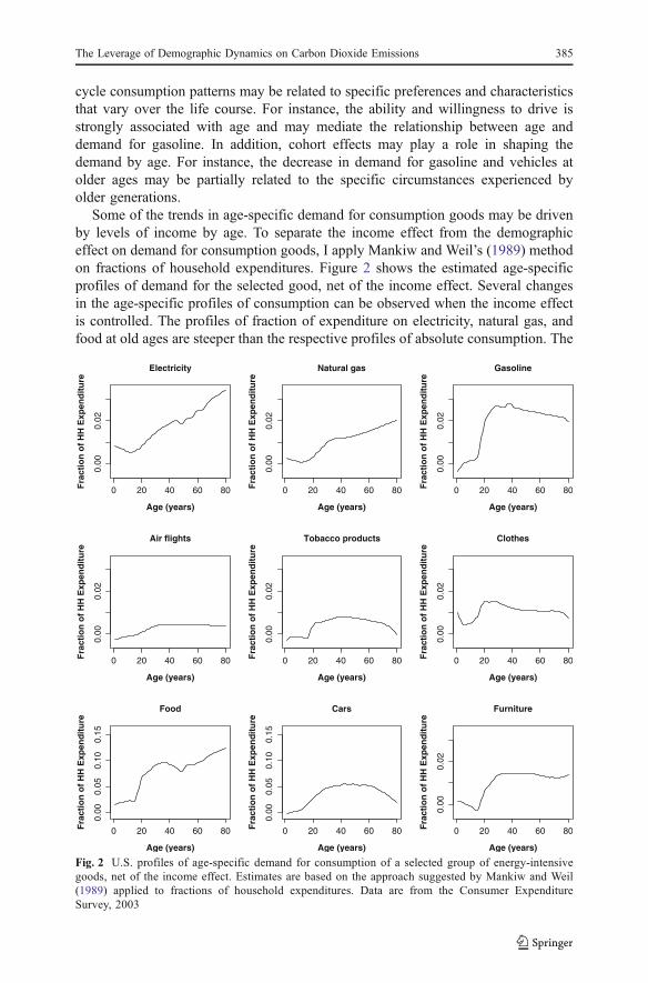
cycle consumption patterns may be related to specific preferences and characteristicsthat vary over the life course. For instance, the ability and willingness to drive isstrongly associated with age and may mediate the relationship between age anddemand for gasoline. In addition, cohort effects may play a role in shaping thedemand by age. For instance, the decrease in demand for gasoline and vehicles atolder ages may be partially related to the specific circumstances experienced byolder generations.

Some of the trends in age-specific demand for consumption goods may be drivenby levels of income by age. To separate the income effect from the demographiceffect on demand for consumption goods, I apply Mankiw and Weil’s (1989) methodon fractions of household expenditures. Figure 2 shows the estimated age-specificprofiles of demand for the selected good, net of the income effect. Several changesin the age-specific profiles of consumption can be observed when the income effectis controlled. The profiles of fraction of expenditure on electricity, natural gas, andfood at old ages are steeper than the respective profiles of absolute consumption. The

0 20 40 60 80

0.00

0.02

Electricity

Age (years)

Fra

ctio

n o

f H

H E

xpen

dit

ure

0 20 40 60 80

0.00

0.02

Natural gas

Age (years)

Fra

ctio

n o

f H

H E

xpen

dit

ure

0 20 40 60 80

0.00

0.02

Gasoline

Age (years)

Fra

ctio

n o

f H

H E

xpen

dit

ure

0 20 40 60 80

0.00

0.02

Air flights

Age (years)

Fra

ctio

n o

f H

H E

xpen

dit

ure

0 20 40 60 80

0.00

0.02

Tobacco products

Age (years)

Fra

ctio

n o

f H

H E

xpen

dit

ure

0 20 40 60 80

0.00

0.02

Clothes

Age (years)

Fra

ctio

n o

f H

H E

xpen

dit

ure

0 20 40 60 80

0.00

0.05

0.10

0.15

Food

Age (years)

Fra

ctio

n o

f H

H E

xpen

dit

ure

0 20 40 60 80

0.00

0.05

0.10

0.15

Cars

Age (years)

Fra

ctio

n o

f H

H E

xpen

dit

ure

0 20 40 60 80

0.00

0.02

Furniture

Age (years)

Fra

ctio

n o

f H

H E

xpen

dit

ure

Fig. 2 U.S. profiles of age-specific demand for consumption of a selected group of energy-intensivegoods, net of the income effect. Estimates are based on the approach suggested by Mankiw and Weil(1989) applied to fractions of household expenditures. Data are from the Consumer ExpenditureSurvey, 2003


opposite is true for gasoline, clothes, cars, and furniture, for which the profiles offraction of expenditure at old ages are rather flat compared with the estimatedprofiles of absolute consumption, which tend to decline fairly rapidly at old ages.The profiles of consumption and fraction of expenditures are rather similar for goodssuch as air flights and tobacco. These observations are potentially relevant forunderstanding implications of changing levels of wealth for the elderly on theirconsumption of energy-intensive goods.

Figure 3 shows estimates of age-specific consumption profiles obtained using theequivalence scale approach that I suggest. These estimated profiles are qualitativelyconsistent with the ones obtained using the Mankiw and Weil (1989) approach. Theyare also consistent with the results obtained by O’Neill and Chen (2002) using adifferent set of data and methods. As a matter of fact, O’Neill and Chen estimatedthat residential energy use rises with the age of the householder, whereastransportation energy use rises to a peak, when the householder is in his early 50s,and then falls to low levels at the oldest ages. In O’Neill and Chen (2002), the unit ofanalysis is the household. Here, I complement their work by estimating profiles for

0 20 40 60 80

020

040

060

0

Electricity

Age (years)

U.S

. Do

llars

0 20 40 60 80

020

040

060

0

Natural gas

Age (years)

U.S

. Do

llars

0 20 40 60 80

020

040

060

0

Gasoline

Age (years)

U.S

. Do

llars

0 20 40 60 80

020

040

060

0

Air flights

Age (years)

U.S

. Do

llars

0 20 40 60 80

020

040

060

0

Tobacco products

Age (years)

U.S

. Do

llars

0 20 40 60 80

020

040

060

0

Clothes

Age (years)

U.S

. Do

llars

0 20 40 60 80

010

0020

0030

00

Food

Age (years)

U.S

. Do

llars

0 20 40 60 80

010

0020

0030

00

Cars

Age (years)

U.S

. Do

llars

0 20 40 60 80

020

040

060

0

Furniture

Age (years)

U.S

. Do

llars

Fig. 3 U.S. annual average expenditure by age for a selected group of energy-intensive goods. Estimatesare obtained using the equivalence scale approach. Data are from the Consumer Expenditure Survey, 2003

386 E. Zagheni

individuals and by quantitatively evaluating the extent of economies of scale inconsumption that arise from cohabitation.

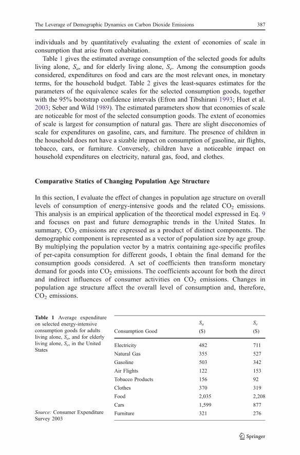
Table 1 gives the estimated average consumption of the selected goods for adultsliving alone, Sa, and for elderly living alone, Se. Among the consumption goodsconsidered, expenditures on food and cars are the most relevant ones, in monetaryterms, for the household budget. Table 2 gives the least-squares estimates for theparameters of the equivalence scales for the selected consumption goods, togetherwith the 95% bootstrap confidence intervals (Efron and Tibshirani 1993; Huet et al.2003; Seber and Wild 1989). The estimated parameters show that economies of scaleare noticeable for most of the selected consumption goods. The extent of economiesof scale is largest for consumption of natural gas. There are slight diseconomies ofscale for expenditures on gasoline, cars, and furniture. The presence of children inthe household does not have a sizable impact on consumption of gasoline, air flights,tobacco, cars, or furniture. Conversely, children have a noticeable impact onhousehold expenditures on electricity, natural gas, food, and clothes.

Comparative Statics of Changing Population Age Structure

In this section, I evaluate the effect of changes in population age structure on overalllevels of consumption of energy-intensive goods and the related CO2 emissions.This analysis is an empirical application of the theoretical model expressed in Eq. 9and focuses on past and future demographic trends in the United States. Insummary, CO2 emissions are expressed as a product of distinct components. Thedemographic component is represented as a vector of population size by age group.By multiplying the population vector by a matrix containing age-specific profilesof per-capita consumption for different goods, I obtain the final demand for theconsumption goods considered. A set of coefficients then transform monetarydemand for goods into CO2 emissions. The coefficients account for both the directand indirect influences of consumer activities on CO2 emissions. Changes inpopulation age structure affect the overall level of consumption and, therefore,CO2 emissions.

Sa Se

Consumption Good ($) ($)

Electricity 482 711

Natural Gas 355 527

Gasoline 503 342

Air Flights 122 153

Tobacco Products 156 92

Clothes 370 319

Food 2,035 2,208

Cars 1,599 877

Furniture 321 276

Table 1 Average expenditureon selected energy-intensiveconsumption goods for adultsliving alone, Sa, and for elderlyliving alone, Se, in the UnitedStates

Source: Consumer ExpenditureSurvey 2003


Age-Specific Profile of CO2 Emissions

I estimated and discussed monetary age-specific profiles of consumption for a set ofrelevant goods in a previous section. In order to carry out a comparative staticsanalysis of the effect of changes in population age structure on CO2 emissions, Ineed a set of coefficients that transforms final demand of goods into CO2 emissions.For this purpose, I follow the approach of Bin and Dowlatabadi (2005). In particular,I use the Environmental Input-Output Life Cycle Analysis model (EIO-LCA 2009;Hendrickson et al. 2006) to estimate the indirect consequences of consumption (i.e.,CO2 emissions that occur during the production and delivery of a product or service,and before its use). As for direct consequences of consumption (i.e., CO2 emissionsthat occur while the product or service is in use), I use the coefficients reported bythe Energy Information Administration (EIA 2009a). Such coefficients are necessaryto account for emissions associated with the use phase of gasoline and natural gas,since the EIO-LCA model accounts only for emissions embedded in the productionof consumption goods but not for emissions associated with the burning of suchfuels when in use. Figure 4 shows estimated CO2 intensity for the set ofconsumption goods under consideration. The estimates, obtained by combininginformation from EIO-LCA (2009) and EIA (2009a), account for both direct andindirect consequences of consumption. Consistent with the work of Bin andDowlatabadi (2005), I observe that the most CO2-intensive consumer activities arerelated to consumption of utilities and personal travel. It is also interesting to note

Consumption Good Equivalence Scale Parameters

g q

Electricity 0.27 0.952

(0.208; 0.325) (0.948; 0.955)

Natural Gas 0.249 0.924

(0.146; 0.341) (0.917; 0.93)

Gasoline 0.054 1.004

(0.013; 0.092) (1.001; 1.008)

Air Flights 0 0.948

(––) (0.935; 0.963)

Tobacco Products 0 0.941

(––) (0.933; 0.953)

Clothes 0.405 0.979

(0.300; 0.498) (0.972; 0.985)

Food 0.223 0.985

(0.170; 0.266) (0.983; 0.988)

Cars 0.087 1.015

(0; 0.174) (1.008; 1.025)

Furniture 0.068 1.004

(0; 0.136) (0.995; 1.014)

Table 2 Estimates of theparameters of the equivalencescale for a selected group ofenergy-intensive consumptiongoods

Notes: Numbers in parenthesesgive the bootstrap 95% confi-dence intervals. g represents therelative consumption of children,with respect to adults. q repre-sents the extent of economies ofscale from cohabitation

Source: Consumer ExpenditureSurvey 2003

388 E. Zagheni

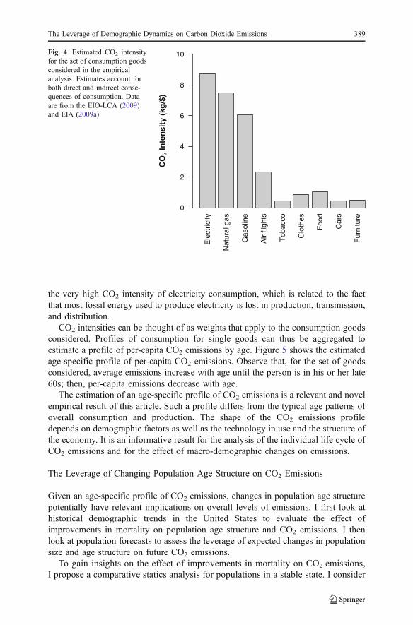
the very high CO2 intensity of electricity consumption, which is related to the factthat most fossil energy used to produce electricity is lost in production, transmission,and distribution.

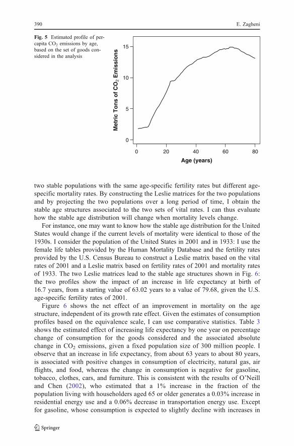
CO2 intensities can be thought of as weights that apply to the consumption goodsconsidered. Profiles of consumption for single goods can thus be aggregated toestimate a profile of per-capita CO2 emissions by age. Figure 5 shows the estimatedage-specific profile of per-capita CO2 emissions. Observe that, for the set of goodsconsidered, average emissions increase with age until the person is in his or her late60s; then, per-capita emissions decrease with age.

The estimation of an age-specific profile of CO2 emissions is a relevant and novelempirical result of this article. Such a profile differs from the typical age patterns ofoverall consumption and production. The shape of the CO2 emissions profiledepends on demographic factors as well as the technology in use and the structure ofthe economy. It is an informative result for the analysis of the individual life cycle ofCO2 emissions and for the effect of macro-demographic changes on emissions.

The Leverage of Changing Population Age Structure on CO2 Emissions

Given an age-specific profile of CO2 emissions, changes in population age structurepotentially have relevant implications on overall levels of emissions. I first look athistorical demographic trends in the United States to evaluate the effect ofimprovements in mortality on population age structure and CO2 emissions. I thenlook at population forecasts to assess the leverage of expected changes in populationsize and age structure on future CO2 emissions.

To gain insights on the effect of improvements in mortality on CO2 emissions,I propose a comparative statics analysis for populations in a stable state. I consider

Ele

ctric

ity

Nat

ural

gas

Gas

olin

e

Air

fligh

ts

Tob

acco

Clo

thes

Foo

d

Car

s

Fur

nitu

re

CO

2 In

ten

sity

(kg

/$)

0

2

4

6

8

10Fig. 4 Estimated CO2 intensityfor the set of consumption goodsconsidered in the empiricalanalysis. Estimates account forboth direct and indirect conse-quences of consumption. Dataare from the EIO-LCA (2009)and EIA (2009a)


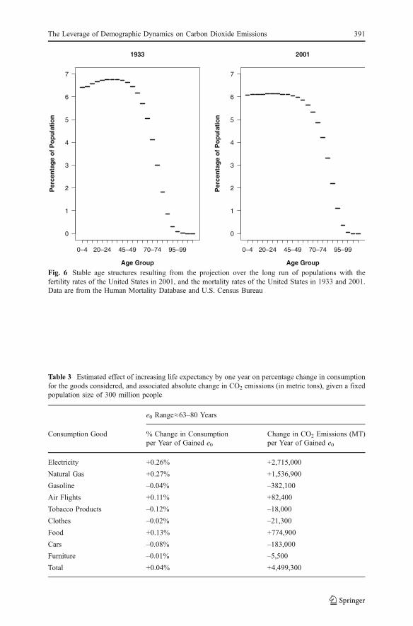
two stable populations with the same age-specific fertility rates but different age-specific mortality rates. By constructing the Leslie matrices for the two populationsand by projecting the two populations over a long period of time, I obtain thestable age structures associated to the two sets of vital rates. I can thus evaluatehow the stable age distribution will change when mortality levels change.

For instance, one may want to know how the stable age distribution for the UnitedStates would change if the current levels of mortality were identical to those of the1930s. I consider the population of the United States in 2001 and in 1933: I use thefemale life tables provided by the Human Mortality Database and the fertility ratesprovided by the U.S. Census Bureau to construct a Leslie matrix based on the vitalrates of 2001 and a Leslie matrix based on fertility rates of 2001 and mortality ratesof 1933. The two Leslie matrices lead to the stable age structures shown in Fig. 6:the two profiles show the impact of an increase in life expectancy at birth of16.7 years, from a starting value of 63.02 years to a value of 79.68, given the U.S.age-specific fertility rates of 2001.

Figure 6 shows the net effect of an improvement in mortality on the agestructure, independent of its growth rate effect. Given the estimates of consumptionprofiles based on the equivalence scale, I can use comparative statistics. Table 3shows the estimated effect of increasing life expectancy by one year on percentagechange of consumption for the goods considered and the associated absolutechange in CO2 emissions, given a fixed population size of 300 million people. Iobserve that an increase in life expectancy, from about 63 years to about 80 years,is associated with positive changes in consumption of electricity, natural gas, airflights, and food, whereas the change in consumption is negative for gasoline,tobacco, clothes, cars, and furniture. This is consistent with the results of O’Neilland Chen (2002), who estimated that a 1% increase in the fraction of thepopulation living with householders aged 65 or older generates a 0.03% increase inresidential energy use and a 0.06% decrease in transportation energy use. Exceptfor gasoline, whose consumption is expected to slightly decline with increases in

0 20 40 60 80

0

5

10

15

Age (years)

Met

ric

To

ns

of

CO

2 E

mis

sio

ns

Fig. 5 Estimated profile of per-capita CO2 emissions by age,based on the set of goods con-sidered in the analysis

390 E. Zagheni

0–4 20–24 45–49 70–74 95–99

0

1

2

3

4

5

6

7

1933

Age Group

Per

cen

tag

e o

f P

op

ula

tio

n

0–4 20–24 45–49 70–74 95–99

0

1

2

3

4

5

6

7

2001

Age Group

Per

cen

tag

e o

f P

op

ula

tio

n

Fig. 6 Stable age structures resulting from the projection over the long run of populations with thefertility rates of the United States in 2001, and the mortality rates of the United States in 1933 and 2001.Data are from the Human Mortality Database and U.S. Census Bureau

Table 3 Estimated effect of increasing life expectancy by one year on percentage change in consumptionfor the goods considered, and associated absolute change in CO2 emissions (in metric tons), given a fixedpopulation size of 300 million people

e0 Range≈63–80 Years

Consumption Good % Change in Consumptionper Year of Gained e0

Change in CO2 Emissions (MT)per Year of Gained e0

Electricity +0.26% +2,715,000

Natural Gas +0.27% +1,536,900

Gasoline –0.04% –382,100

Air Flights +0.11% +82,400

Tobacco Products –0.12% –18,000

Clothes –0.02% –21,300

Food +0.13% +774,900

Cars –0.08% –183,000

Furniture –0.01% –5,500

Total +0.04% +4,499,300


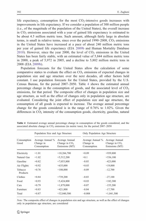
life expectancy, consumption for the most CO2-intensive goods increases withimprovements in life expectancy. If we consider a population of 300 million people(i.e., of the magnitude of the population of the United States), the overall increasein CO2 emissions associated with a year of gained life expectancy is estimated tobe about 4.5 million metric tons. Such amount, although fairly large in absoluteterms, is small in relative terms, since over the period 1990–2008, CO2 emissionsin the United States have increased at a pace of about 240 million metric tonsper year of gained life expectancy (EIA 2009b and Human Mortality Database2010). However, since the year 2000, the level of CO2 emissions in the UnitedStates has been fairly stable, with an estimated value of 5,844 million metric tonsin 2000, a peak of 5,972 in 2005, and a decline to 5,802 million metric tons in2008 (EIA 2009b).

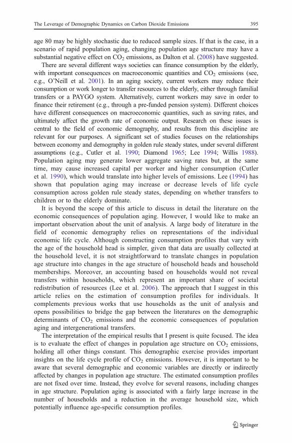
Population forecasts for the United States allow the calculation of somecomparative statics to evaluate the effect on CO2 emissions of expected changes inpopulation size and age structure over the next decades, all other factors heldconstant. I use population forecasts for the United States, provided by the U.S.Census Bureau, for the period 2007–2050. Table 4 shows the estimated annualpercentage change in the consumption of goods, and the associated level of CO2

emissions, for that period. The composite effect of changes in population size andage structure, as well as the effect of changes only in population age structure, areevaluated. Considering the joint effect of population size and age structure, theconsumption of all goods is expected to increase. The average annual percentagechange for the goods considered is in the range of 0.76% to 1.02%. Given thedifferences in CO2 intensity of the consumption goods, electricity, gasoline, natural

Table 4 Estimated average annual percentage change in consumption of the goods considered, and theassociated absolute change in CO2 emissions (in metric tons), for the period 2007–2050

Population Size and Age Structure Only Population Age Structure

ConsumptionGood

Average Annual %Change inConsumption

Average AnnualChange in CO2

Emissions (MT)

Average Annual %Change inConsumption

Average AnnualChange in CO2

Emissions (MT)

Electricity +1.01 +10,266,700 +0.09 +939,800

Natural Gas +1.02 +5,512,200 +0.1 +536,100

Gasoline +0.82 +7,053,800 –0.05 –423,000

Air Flights +0.92 +635,000 +0.03 +19,000

TobaccoProducts

+0.76 +108,000 –0.09 –12,700

Clothes +0.84 +739,200 –0.03 –27,100

Food +0.93 +5,424,800 +0.03 +182,300

Cars +0.79 +1,879,000 –0.07 –155,200

Furniture +0.83 +421,800 –0.04 –17,700

Total +0.87 +32,040,500 –0.008 +1,041,500

Note: The composite effect of changes in population size and age structure, as well as the effect of changesonly in population age structure, are considered

392 E. Zagheni

gas, and food account for most of the expected average annual change in CO2

emissions, which is estimated to be about 32 million metric tons. When I consideronly the effect of population age structure, I observe that the overall average annualpercentage change in consumption is slightly negative. However, increases areexpected in consumption for the most CO2-intensive goods except for gasoline.Electricity and natural gas consumption are expected to increase by about 0.1%per year, whereas consumption of gasoline is expected to decrease by 0.05% peryear due to changes in age structure. This is consistent with the results ofO’Neill and Chen (2002), who projected an age-driven percentage change inresidential energy consumption of between +2% and +5% for the period 2000–2050. They also projected an age-driven percentage change in transportationenergy consumption of between –1% and 0% for the same period. The expectedincrease in consumption of the most CO2-intensive goods, due to changes inpopulation age structure, leads to an average annual estimated increase in CO2

emissions of about 1 million metric tons.The comparative statics exercise gives a general idea of the importance of a

demographic factor, such as age distribution, in the explanation of energyrequirements and CO2 emissions of an economy like the United States’. Theimpact of changing age distribution is fairly small in relative terms, consideringthat, in the United States, the estimated annual CO2 emissions are in the order of5,800 million metric tons and that large gains in terms of life expectancy mayoccur over a rather long period of time. However, the impact of changing agedistribution is relevant in absolute terms, and particularly noticeable, consideringthat the level of emissions in the United States has been fairly stable over the pastfew years.

Discussion

In this article, I discuss the effect of changing population age structure on CO2

emissions. Methodologically, I first proposed a generalization of the well-knownIPAT equation to account for the role of population age structure and inter-relationships between sectors of the economy. Second, I developed a statisticalmodel to estimate the extent of economies of scale in consumption that arise fromcohabitation. Third, I suggested a technique to estimate age-specific consumptionprofiles from data on household expenditure and household composition. Empiri-cally, I offered an application of the methods, based on a set of CO2-intensive goodsfor the United States. I found that per-capita CO2 emissions increase with age untilthe individual is in his or her 60s. Then, per-capita CO2 emissions tend to decline.Improvements in life expectancy and low levels of fertility shift the distribution ofperson-years lived toward old ages. An exercise of comparative statics shows thatthis process has a positive, although rather small, effect on CO2 emissions in the nextfew decades. In the longer term, when the proportion of person-years lived at veryold ages increases, the effect may become negative, given the estimated age-specificprofile of CO2 emissions.

The empirical analysis performed in the paper mainly serves as an illustrationof the methodological contribution and does not represent a comprehensive


account of all consumption goods in the economy. However, the goods havebeen chosen based on their relevance in terms of CO2 emissions and account for alarge part of CO2 emissions in the United States, making the results fairly general.The proposed model and empirical analysis provide a systematization of previousIPAT-based studies that evaluate the effect of population age composition andeconomic structure on CO2 emissions (e.g., Dietz and Rosa 1994; Fan et al. 2006;Mackellar et al. 1995; Shi 2003). The previous IPAT-based literature on the topicrelied on simple measures of age composition and economic structure and did notcome to conclusive evidence on their effect on CO2 emissions. This study providesa more articulated framework to interpret previous IPAT-based literature and tofurther develop analytic tools and empirical strategies to evaluate the relationshipsbetween demographic dynamics and CO2 emissions. The empirical results seem toconfirm the recent findings of Fan et al. (2006) that the effect of population agecomposition is related to the economic structure of the economy, and that, in high-income countries, aging has a positive effect on CO2 emissions, at least in therelatively short term.

The estimated age-specific consumption profiles show a pattern of residentialenergy use consistent with the one estimated by O’Neill and Chen (2002) for the lifecycle of households. The effect of changing population age structure on CO2

emissions has also been evaluated in literature that relies on energy-economicgrowth models. The benchmark study in this area of research is given by Daltonet al. (2008). They used a general equilibrium model with multiple dynasties ofheterogeneous households, calibrated with input-output data, to evaluate the effect ofaging on CO2 emissions in the United States. The model that they proposed can bethought of, to a certain extent, as a dynamic version of the static model that I suggestin this article. They found that population aging reduces long-term emissions. Theeffect of aging on per-capita emissions is not apparent until after 2050 because ofpopulation momentum. In the Dalton et al. model, the most relevant impacts ofaging are caused by differentials in labor income across age groups, which generatecomplex dynamics for consumption and savings. Their results are driven mainly bythe crucial assumption that per-capita labor force participation is fixed over time.Population aging and the scarcity of young workers then cause a downward trend inper-capita labor income for dynasties, with relevant consequences on per-capitaconsumption and CO2 emissions. The assumption is fairly strong, since it is likelythat people in the older age groups will increase their labor force participation, bothbecause of improved health conditions at older ages and because of pressures on thepension system that will translate into increases in the age at retirement or in thenumber of hours worked. In this article, I implicitly assume that estimatedconsumption profiles are sustainable and that the economy will adjust to populationaging through changes in labor force participation or the number of hours worked.Relaxing the assumption of fixed labor force participation in Dalton et al. (2008)would likely reduce the difference between their projections for the relatively shortterm and the results that I present. In the long term, the reduction in CO2 emissionsdue to aging, suggested by Dalton et al. (2008), is consistent with the age-specificprofile of CO2 emissions that I estimate and that implies a decrease in CO2 emissionsat very old ages. There are indications that consumption of energy-intensive goodskeeps decreasing at very old ages, although estimates of consumption profiles past

394 E. Zagheni

age 80 may be highly stochastic due to reduced sample sizes. If that is the case, in ascenario of rapid population aging, changing population age structure may have asubstantial negative effect on CO2 emissions, as Dalton et al. (2008) have suggested.

There are several different ways societies can finance consumption by the elderly,with important consequences on macroeconomic quantities and CO2 emissions (see,e.g., O’Neill et al. 2001). In an aging society, current workers may reduce theirconsumption or work longer to transfer resources to the elderly, either through familialtransfers or a PAYGO system. Alternatively, current workers may save in order tofinance their retirement (e.g., through a pre-funded pension system). Different choiceshave different consequences on macroeconomic quantities, such as saving rates, andultimately affect the growth rate of economic output. Research on these issues iscentral to the field of economic demography, and results from this discipline arerelevant for our purposes. A significant set of studies focuses on the relationshipsbetween economy and demography in golden rule steady states, under several differentassumptions (e.g., Cutler et al. 1990; Diamond 1965; Lee 1994; Willis 1988).Population aging may generate lower aggregate saving rates but, at the sametime, may cause increased capital per worker and higher consumption (Cutleret al. 1990), which would translate into higher levels of emissions. Lee (1994) hasshown that population aging may increase or decrease levels of life cycleconsumption across golden rule steady states, depending on whether transfers tochildren or to the elderly dominate.

It is beyond the scope of this article to discuss in detail the literature on theeconomic consequences of population aging. However, I would like to make animportant observation about the unit of analysis. A large body of literature in thefield of economic demography relies on representations of the individualeconomic life cycle. Although constructing consumption profiles that vary withthe age of the household head is simpler, given that data are usually collected atthe household level, it is not straightforward to translate changes in populationage structure into changes in the age structure of household heads and householdmemberships. Moreover, an accounting based on households would not revealtransfers within households, which represent an important share of societalredistribution of resources (Lee et al. 2006). The approach that I suggest in thisarticle relies on the estimation of consumption profiles for individuals. Itcomplements previous works that use households as the unit of analysis andopens possibilities to bridge the gap between the literatures on the demographicdeterminants of CO2 emissions and the economic consequences of populationaging and intergenerational transfers.

The interpretation of the empirical results that I present is quite focused. The ideais to evaluate the effect of changes in population age structure on CO2 emissions,holding all other things constant. This demographic exercise provides importantinsights on the life cycle profile of CO2 emissions. However, it is important to beaware that several demographic and economic variables are directly or indirectlyaffected by changes in population age structure. The estimated consumption profilesare not fixed over time. Instead, they evolve for several reasons, including changesin age structure. Population aging is associated with a fairly large increase in thenumber of households and a reduction in the average household size, whichpotentially influence age-specific consumption profiles.


Population aging also affects productivity. For instance, old workers may be moreexperienced and productive than younger ones. Conversely, it is possible that youngworkers are more dynamic and productive. Depending on which effect is stronger,productivity may increase or decrease with age, with consequences on economicgrowth and consumption patterns. My estimates of consumption profiles are basedon cross-sectional data and are influenced by the pace of economic growth. Rapideconomic growth raises the income of young people, relative to the elderly, andmakes longitudinal profiles of consumption steeper than the ones estimated fromcross-sectional data.

Technology is an important variable in the explanation of CO2 emissions. Theapproach used in this article is based on a static representation of technology (e.g.,the input-output model). However, technical change may play a key role in thefuture. For instance, reducing the CO2 intensity of electricity may counteract the effectof increasing consumption due to population aging. On the other hand, internationaltrade may shift the production of certain goods to countries where the technology inuse is more energy-intensive, thus leading to an overall increase in CO2 emissionswhich is not captured by input-output tables that do not account for trade.

In this article, I focus on the United States and formalize the intuition thatobserved patterns of energy use in developed countries imply that population agingmay have a positive impact on CO2 emissions (e.g., Haq et al. 2007). I also offerinsights for a country like China, one of the main contributors to global CO2

emissions. In China, the process of population aging is extremely fast and is likely tohave a significant impact on CO2 emissions. In particular, population aging comestogether with rapid economic growth, which will likely increase the overall level ofconsumption and will make the age-specific profiles increase more steeply with age.Changes in age structure potentially have large consequences in developingcountries and, more generally, on global CO2 emissions. In the context of adeveloping country, however, it is important to consider the process of aging andreduction in household size together with urbanization. As a matter of fact, theprocesses of economic development and urbanization is expected to drive CO2

emissions in countries like China and India (Dalton et al. 2007) and need furtherconsideration for estimation and prediction of global CO2 emissions.

Further research must be pursued in order to inform official forecasts for CO2

emissions with an improved understanding of the role of demographic dynamics. Inparticular, I think that interdisciplinary work to bring together different areas ofexpertise will be central to improving our understanding of the impact of populationdynamics on CO2 emissions in both developed and developing countries.

Acknowledgements I am greatly indebted to Ronald Lee and Kenneth Wachter for their insightfulcomments throughout the development of this study. I am also very grateful to two anonymous reviewers,whose suggestions helped me to considerably improve the manuscript. Early versions of the article alsobenefited from the valuable comments of John Rice, Dowell Myers, Francesco Billari, Rebecca Clark,Donald Hastings, and from conversations with graduate students at the Department of Demography of theUniversity of California, Berkeley.

Open Access This article is distributed under the terms of the Creative Commons AttributionNoncommercial License which permits any noncommercial use, distribution, and reproduction in anymedium, provided the original author(s) and source are credited.

396 E. Zagheni

References

Bin, S., & Dowlatabadi, H. (2005). Consumer lifestyle approach to U.S. energy use and the related CO2

emissions. Energy Policy, 33, 197–208.Chertow, M. R. (2001). The IPAT equation and its variants. Journal of Industrial Ecology, 4(4), 13–

29.Commoner, B. (1972). The environmental cost of economic growth. In R. G. Ridker (Ed.), Population,

resources and the environment (pp. 339–364). Washington, DC: U.S. Government Printing Office.Cutler, D., Poterba, J., Sheiner, L., & Summers, L. (1990). An aging society: Opportunity or challenge?

Brookings Papers on Economic Activity, 1, 1–73.Dalton, M., Jiang, L., Pachauri, S., & O’Neill, B. C. (2007). Demographic change and future carbon

emissions in China and India. Paper presented at the annual meeting of the Population Association ofAmerica, March 29–31, New York.

Dalton, M., O’Neill, B. C., Prskawetz, A., Jiang, L., & Pitkin, J. (2008). Population aging and futurecarbon emissions in the United States. Energy Economics, 30, 642–675.

Diamond, P. A. (1965). National debt in a neoclassical growth model. American Economic Review, 55, 1126–1150.

Dietz, T., & Rosa, E. A. (1994). Rethinking the environmental impacts of population, affluence andtechnology. Human Ecology Review, 1, 277–300.

Dietz, T., & Rosa, E. A. (1997). Effects of population and affluence on CO2 emissions. Proceedings of theNational Academy of Sciences of the USA, 94, 175–179.

Duchin, F. (1996). Population change, lifestyle and technology: How much difference can they make?Population and Development Review, 22, 321–330.

Duchin, F. (1998). Structural economics: Measuring change in technology, lifestyles, and the environment.Washington, DC: Island Press.

Duchin, F., & Lange, G. M. (1994). The future of the environment: Ecological economics andtechnological change. New York: Oxford University Press.

Efron, B., & Tibshirani, R. J. (1993). An Introduction to the Bootstrap. Monographs on Statistics andApplied Probability 57. Chapman & Hall/Crc.

Ehrlich, P., & Holdren, J. (1971). Impact of population growth. Science, 171, 1212–1217.Ehrlich, P., & Holdren, J. (1972). Impact of population growth. In R. G. Ridker (Ed.), Population,

resources and the environment (pp. 365–378). Washington, DC: U.S. Government Printing Office.EIO-LCA. (2009). Economic input-output life cycle assessment (EIO-LCA) Model. Carnegie Mellon

University Green Design Institute. Available online at http://www.eiolca.net.Energy Information Administration (EIA). (2009a). Emissions factors and global warming potentials. EIA,

Department of Energy. Available online at http://www.eia.doe.gov/oiaf/1605/emission_factors.html.Energy Information Administration (EIA). (2009b). U.S. Carbon Dioxide Emissions From Energy Sources

2008 Flash Estimate. EIA, Department of Energy. Available online at http://www.eia.doe.gov/oiaf/1605/flash/flash.html.

Fan, Y., Liu, L. C., Wu, G., & Wei, Y. M. (2006). Analyzing impact factors of CO2 emissions using theSTIRPAT model. Environmental Impact Assessment Review, 26, 377–395.

Friedman, J. H. (1984). A variable span scatterplot smoother. Laboratory for Computational Statistics,Stanford University Technical Report No. 5.

Haq, G., Minx, J., Whitelegg, J., Owen, A. (2007). Greening the greys: Climate change and the over 50s.Report of the Stockholm Environment Institute, University of York.

Hendrickson, C. T., Lave, L. B., & Matthews, H. S. (2006). Environmental life cycle assessment of goodsand services, an input-output approach. Washington, DC: Resources for the Future.

Hertwich, E. G. (2005). Life cycle approaches to sustainable consumption: A critical review.Environmental Science and Technology, 39, 4673–4684.

Herzog, H. W., Jr., & Ridker, R. G. (1972). The model. In R. G. Ridker (Ed.), Population, resources andthe environment (pp. 301–312). Washington, DC: U.S. Government Printing Office.

Huet, S., Bouvier, A., Poursat, M. A., & Jolivet, E. (2003). Statistical tools for nonlinear regression. NewYork: Springer.

Human Mortality Database. (2010). University of California, Berkeley (USA), and Max Planck Institute forDemographic Research (Germany). Available online at www.mortality.org or www.humanmortality.de.

Intergovernmental Panel on Climate Change (IPCC). (2007). Intergovernmental panel on climate change.Climate Change 2007. Fourth Assessment Report. Un-edited Copy Prepared for COP-13.

Keyfitz, N., & Caswell, H. (2005). Applied mathematical demography. New York: Springer.


http://www.eiolca.net

http://www.eia.doe.gov/oiaf/1605/emission_factors.html

http://www.eia.doe.gov/oiaf/1605/flash/flash.html

http://www.eia.doe.gov/oiaf/1605/flash/flash.html

http://www.mortality.org

http://www.humanmortality.de

Lee, R. (1994). The formal demography of population aging, transfers, and the economic life cycle. In L.G. Martin & S. H. Preston (Eds.), The demography of aging (pp. 8–49). Washington, DC: NationalAcademy Press.

Lee, R. (2000). A cross-cultural perspective on intergenerational transfers and the economic life cycle. InA. Mason & G. Tapinos (Eds.), Sharing the Wealth: Demographic change and economic transfersbetween generations (pp. 17–56). Oxford: Oxford University Press.

Lee, R., Lee, S. H., & Mason, A. (2006). Charting the economic life cycle, NBER working paper No.W12379. Cambridge, MA: National Bureau of Economic Research.

Lenzen, M. (1998). Primary energy and greenhouse gases embodied in Australian final consumption: Aninput-output analysis. Energy Policy, 26, 495–506.

Leontief, W. (1936). Quantitative input and output relations in the economic system of the United States.Review of Economics and Statistics, 18(3), 105–125.

Leontief, W. (1953). Studies in the structure of the American economy. New York: Oxford UniversityPress.

Leontief, W. (1970). Environmental repercussions and the economic structure: An input-output approach.Review of Economics and Statistics, 52(3), 262–271.

Leontief, W. (1986). Input-output economics. New York: Oxford University Press.MacKellar, F. L., Lutz, W., Prinz, C., & Goujon, A. (1995). Population, households and CO2 emissions.

Population and Development Review, 21, 849–865.Mankiw, N. G., & Weil, D. N. (1989). The baby boom, the baby bust, and the housing market. Regional

Science and Urban Economics, 19, 235–258.O’Neill, B. C. (2005). The role of demographics in emissions scenarios. Extended Abstract published

in Meeting Report: IPCC Expert Meeting on Emissions Scenarios, 12–14 January, Washington,DC.

O’Neill, B. C., & Chen, B. S. (2002). Demographic determinants of household energy use in the UnitedStates. Population and Development Review, 28, 53–88.

O’Neill, B. C., MacKellar, F. L., & Lutz, W. (2001). Population and climate change. Cambridge, UK:Cambridge University Press.

Pachauri, S., & Spreng, D. (2002). Direct and indirect energy requirements of households in India. EnergyPolicy, 30, 511–523.

Pebley, A. R. (1998). Demography and the environment. Demography, 35, 377–389.Peters, G. P., & Hertwich, E. G. (2006). The importance of imports for household environmental impacts.

Journal of Industrial Ecology, 10(3), 89–109.Peters, G. P., & Hertwich, E. G. (2008). Post-Kyoto greenhouse gas inventories: Production versus

consumption. Climatic Change, 86, 51–66.Preston, S. H. (1996). The effect of population growth on environmental quality. Population Research and

Policy Review, 15, 95–108.Reinders, A. H. M. E., Vringer, K., & Blok, K. (2003). The direct and indirect energy requirement of

households in the European union. Energy Policy, 31, 139–153.Ridker, R. G. (1972). Resource and environmental consequences of population growth in the United

States: A summary. In R. G. Ridker (Ed.), Population, resources and the environment (pp. 17–34).Washington, DC: U.S. Government Printing Office.

Rosa, E. A., York, R., & Dietz, T. (2004). Tracking the anthropogenic drivers of ecological impacts.Ambio, 33, 509–512.

Ruttan, V. W. (1993). Population growth, environmental change, and innovation: Implications forsustainable growth in agriculture. In C. L. Jolly & B. B. Torrey (Eds.), Population and land use indeveloping countries (pp. 124–156). Washington, DC: National Academy Press.

Schipper, L. (1996). Lifestyles and the environment: The case of energy. Daedalus, 125, 113–138.Schipper, L., Bartlett, S., Hawk, D., & Vine, E. (1989). Linking life-styles and energy use: A matter of

time? Annual Review of Energy, 14, 271–320.Seber, G. A. F., & Wild, C. J. (1989). Nonlinear regression. Hoboken, NJ: John Wiley and Sons, Inc.Shi, A. (2003). The impact of population pressure on global carbon dioxide emissions, 1975–1996:

Evidence from pooled cross-country data. Ecological Economics, 44, 29–42.Solow, R. M. (1956). A contribution to the theory of economic growth. Quarterly Journal of Economics,

70, 65–94.Tukker, A., & Jansen, B. (2006). Environmental impacts of products: A detailed review of studies. Journal

of Industrial Ecology, 10, 159–182.Vringer, K., & Blok, K. (1995). The direct and indirect energy requirement of households in the

Netherlands. Energy Policy, 23, 893–905.

398 E. Zagheni

Waggoner, P. E., & Ausubel, J. H. (2002). A framework for sustainability science: A renovated IPATidentity. Proceedings of the National Academy of Sciences, 99, 7860–7865.

Willis, R. (1988). Life cycles, institutions and population growth: A theory of the equilibrium interest ratein an overlapping-generations model. In R. Lee, W. B. Arthur, & G. Rodgers (Eds.), Economics ofchanging age distributions in developed countries (pp. 106–138). New York: Oxford UniversityPress.

York, R., Rosa, E. A., & Dietz, T. (2003). STIRPAT, IPAT and ImPACT: Analytic tools for unpacking thedriving forces of environmental impacts. Ecological Economics, 46, 351–365.

Zagheni, E., & Billari, F. C. (2007). A cost valuation model based on a stochastic representation of theIPAT equation. Population and Environment, 29, 68–82.


The Leverage of Demographic Dynamics on Carbon Dioxide ... · PDF fileThe Leverage of...

Documents

Transcript of The Leverage of Demographic Dynamics on Carbon Dioxide ... · PDF fileThe Leverage of...