The Langevin Equation: With Applications to Stochastic ... · 3.2. Ornstein-Uhlenbeck theory of...
24
CHAPTER3 BROWNIAN MOTION OF A FREE PARTICLE AND A HARMONIC OSCILLATOR 3.1. Introduction In this chapter, we treat the translational Brownian motion of both a free particle and an oscillator. The appropriate Langevin equations are mi(t)+(x(t)=F(t) (3.1.1) for a free particle, and mi(t) + ( x(t) + mm; x(t) = F(t) (3.1.2) for a Brownian oscillator, where x(t) specifies the position of the particle or oscillator at time t, m is the mass, ( x is the viscous drag experienced by the particle, lVo is the oscillator frequency, and F(t) is the white-noise driving force. We also consider the rotational analogs of these two models, namely, a free single-axis rotator and a torsional oscillator. The corresponding Langevin equations are IB(t) + qO(t) = -t(t) (3.1.3) for a free rotator, and IB(t)+q0(t)+I%B(t) = -t(t) (3.1.4) for a torsional oscillator, where (} is the angle of rotation, I is the moment of inertia, while qB(t) and -t(t) are the viscous drag and white-noise driving torques, respectively. The common feature of all these models is that the Langevin equations (3.1.1 )-{3.1.4) are linear, so that the calculation of observables is relatively simple. Detailed treatments of various aspects of the models are given, e.g., in Refs. [1]-[6] and [6]-[10] for both the translational and rotational Brownian motion. Some properties have already been considered in Chapter 1 (see Sections 1.3 and 1.11). We now show how observables may be calculated from the Langevin equations, Eqs. (3.1.1)-{3.1.4). Applications of the models to the phase diffusion 229 The Langevin Equation Downloaded from www.worldscientific.com by NATIONAL TAIWAN UNIVERSITY on 03/27/14. For personal use only.
Transcript of The Langevin Equation: With Applications to Stochastic ... · 3.2. Ornstein-Uhlenbeck theory of...

CHAPTER3
BROWNIAN MOTION OF A FREE PARTICLE AND A HARMONIC OSCILLATOR
3.1. Introduction
In this chapter, we treat the translational Brownian motion of both a free particle and an oscillator. The appropriate Langevin equations are
mi(t)+(x(t)=F(t) (3.1.1)
for a free particle, and
mi(t) + ( x(t) + mm; x(t) = F(t) (3.1.2)
for a Brownian oscillator, where x(t) specifies the position of the particle or oscillator at time t, m is the mass, ( x is the viscous drag experienced by the particle, lVo is the oscillator frequency, and F(t) is the white-noise driving force. We also consider the rotational analogs of these two models, namely, a free single-axis rotator and a torsional oscillator. The corresponding Langevin equations are
IB(t) + qO(t) = -t(t) (3.1.3)
for a free rotator, and
IB(t)+q0(t)+I%B(t) = -t(t) (3.1.4)
for a torsional oscillator, where (} is the angle of rotation, I is the moment of inertia, while qB(t) and -t(t) are the viscous drag and white-noise driving torques, respectively.
The common feature of all these models is that the Langevin equations (3.1.1 )-{3.1.4) are linear, so that the calculation of observables is relatively simple. Detailed treatments of various aspects of the models are given, e.g., in Refs. [1]-[6] and [6]-[10] for both the translational and rotational Brownian motion. Some properties have already been considered in Chapter 1 (see Sections 1.3 and 1.11 ).
We now show how observables may be calculated from the Langevin equations, Eqs. (3.1.1)-{3.1.4). Applications of the models to the phase diffusion
229
The
Lan
gevi
n E
quat
ion
Dow
nloa
ded
from
ww
w.w
orld
scie
ntif
ic.c
omby
NA
TIO
NA
L T
AIW
AN
UN
IVE
RSI
TY
on
03/2
7/14
. For
per
sona
l use
onl
y.
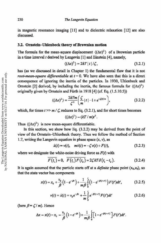
230 The Langevin Equation
in magnetic resonance imaging [11] and to dielectric relaxation [12] are also
discussed.
3.2. Ornstein-Uhlenbeck theory of Brownian motion
The formula for the mean-square displacement ( (1~xY) of a Brownian particle in a time interval t derived by Langevin [1] and Einstein [4], namely,
((Ax)2 )=2kTitil(, (3.2.1)
has (as we discussed in detail in Chapter 1) the fundamental flaw that it is not root-mean-square differentiable at t = 0. We have also seen that this is a direct consequence of ignoring the inertia of the particles. In 1930, Uhlenbeck and Ornstein [2] derived, by including the inertia, the famous formula for ((Ax)2) originally given by Ornstein and Fiirth in 1918 [4] (cf. Eq. (1.5.10.5))
((Ax)2) = 2~m (~It 1-l+e_,ltll., J. (3.2.2)
which, for times t >> m I~ reduces to Eq. (3.2.1), and for short times becomes
((Ax)2) = (kT I m)t2.
Thus ((tix)2) is now mean-square differentiable.
In this section, we show how Eq. (3.2.2) may be derived from the point of view of the Omstein-Uhlenbeck theory. Thus we follow the method of Section 1.7, writing the Langevin equation in phase space (x, v), as
.i(t) = v(t), mv(t) = -( v(t) + F(t),
where we designate the white-noise driving force as F(t) with
F(t1 ) = 0, F(t1 )F(t2 ) = 2(kTo(t1 -t2 ).
(3.2.3)
(3.2.4)
It is again assumed that the particle starts off at a definite phase point (Xo,vo), so that the state vector has components
v 1 t x(t) = x0 + p (t-e-P') + mp [ (1- e-P<r-r'J )F(t')dt', (3.2.5)
v(t) = x(t) = Voe-Pt +...!... j e-P(t-t') F(t')dt' mo
(here P= (I m). Hence
V 1 I
Ax= x(t)- x0 = ~ { 1-e-Pt) +-J [ 1-e-P<r-t'J J F(t')dt'. P mPo
(3.2.6)
The
Lan
gevi
n E
quat
ion
Dow
nloa
ded
from
ww
w.w
orld
scie
ntif
ic.c
omby
NA
TIO
NA
L T
AIW
AN
UN
IVE
RSI
TY
on
03/2
7/14
. For
per
sona
l use
onl
y.

Brownian Motion of a Free Particle and a Harmonic Oscillator 231
Now
(3.2.7)
2 1 t t
(~)2 = ;2 ( 1- e-.Dt r + m2 p2 H [ 1-e-P(t-t')] [ 1-e-P(t-t')] F(t')F(t") dt'dt•
= fJv~ (1-e-ptr + 2kT j j[t-e-P<t-t'>][1-e-JI<t-t') J o(t• -t')dt'dt•. (3.2.8) mfJ o o
Since t I o(t• -t')[1-e-P<t-t')]dt• =1-e-JI(t-t')' (3.2.9) 0
we have, from Eq. (3.2.8),
(~ )2 = :2 ( 1-e -Pt r + 2~: ! [ 1-2e -P(I-1') + e -2J1(t-t')] dt'
_ v; (1 -.Dt )2 2kTt kT [ 3 4e-Pt -2.Dt J -- -e +--+-- - + -e . p2 mfJ mfJ2
(3.2.10)
This is the solution in the case where the collection of particles started off with the definite velocity v0 • If we have a Maxwellian distribution of initial velocities v0, i.e., m(v;) /2 = kT 12, we find from Eq. (3.2.10) that
((~)2)= 2k~ (flt-l+e-.Dt), (3.2.11) mfJ
which is the Ornstein-FUrth formula, Eq. (3.2.2) [2]. For long times, the term in tis the only significant one, so that we obtain the result of Langevin [1] and Einstein [4], Eq. (3.2.1). We reiterate that ((~)2 )112 from Eq. (3.2.11) is nondifferentiable at t = 0 , so that in the non-inertial approximation, the velocity does not exist. If inertia is included, however, ((~)2 )112 is differentiable at t = 0 and the velocity exists. This question, first emphasized by Doob [13], was discussed in Chapter 2.
3.3. Stationary solution of the Langevin equation: the Wiener-Khinchin theorem
We have illustrated the calculation of the averages from the Langevin equation for sharp initial conditions. The solution of the Langevin equation for a free
The
Lan
gevi
n E
quat
ion
Dow
nloa
ded
from
ww
w.w
orld
scie
ntif
ic.c
omby
NA
TIO
NA
L T
AIW
AN
UN
IVE
RSI
TY
on
03/2
7/14
. For
per
sona
l use
onl
y.

232 The Langevin Equation
particle subject to a Maxwellian distribution of velocities is called the stationary solution. Clearly, for the stationary solution
(v2) = kT' (3.3.1) m
as the velocities are in thermal equilibrium. The relevant quantity is the velocity correlation function. The stationary solution may be found by extending the lower limit of integration to --oo and discarding the term in v0 in Eq. (3.2.6). Thus, for distinct times t1 and t2, we have
~ ,. v(t
1) = m-1 I e-P(~-t') F(t')dt', v(t
2) = m-1 I e-P(to-t') F(t•)at• (3.3.2)
so that
(3.3.3)
The modulus bars must be inserted in order to ensure a decaying covariance. This is the velocity autocorrelation function (ACF) of a free Brownian particle. Noting that
t
!.._ (A%)2 = 2Ax(t)v(t), dt
Ax(t) =I v(u)du,
the mean-square displacement ((A%)2) may be found using the formula
t t' t
((A%)2) = 2I I (v(t')v(u)) du dt' = 2I (t-u) (v(O)v(u))du 0 0
yielding the same result as before, Eq. (3.2.11).
(3.3.4)
(3.3.5)
Now the velocity ACF may also be computed using the Wiener-Khinchin theorem. Following Ref. [3] closely, consider, for a very long time T', a widesense stationary random process; that is, a process in which the average of the product ~(t)~(t ± -r) depends only on • (> 0), where we specify the process by the real-valued random variable ~(t) which is a causal function of the time t (see examples in Ref. [14]). We now form
- 1 TI'/2 ~(t) = lim - ~(t)dt,
T'->oo T' -T'/2 (3.3.6)
The
Lan
gevi
n E
quat
ion
Dow
nloa
ded
from
ww
w.w
orld
scie
ntif
ic.c
omby
NA
TIO
NA
L T
AIW
AN
UN
IVE
RSI
TY
on
03/2
7/14
. For
per
sona
l use
onl
y.

Brownian Motion of a Free Particle and a Harmonic Oscillator 233
i.e., the time average of ~(t) over an infinitely long time period. We may also
define the ACF C~( -r) as
C~(-r)=~(t)~(t+-r)= lim_!_ T ~(t)~(t+-r)dt. (3.3.7) T'-+., T' -T'/2
However, the ensemble averages (i.e., the average behavior of a huge ensemble of such stochastic systems observed simultaneously) and time averages are now equal (ergodic theorem), viz.,
c, (-r) = (~(t)~(t+-r)) = ~(t)~(t+ -r). (3.3.8)
Since
~(t)=-1 j ~(m)~""dm and ~((i})= j ~(t)e-iiJJtdt, 27r--«> --«>
(3.3.9)
we have, using the shift theorem for Fourier transforms,
C (-r)= lim_!_ Ts'/2 s"" ~((i})etO}t dOJ s"' e'"''(I+<)~(m,_)dm,_dt. ~ T'-+oO T' 27r 27r
-T'/2-<10 -(I)
(3.3.10)
Because 1 ., - J El~xy dy = t5(x),
27r--«> (3.3.11)
on performing the integration over the t and m,. variables, we obtain
C~(-r)= lim_!_ j j ~((i})~(m,.) e;"'~~t?(m,_ +(i})dmdm,_ T'-+"' T' --«>--«> 27r
• "'s - - . =lim- ~(m)~(-(i})e-'1/n' d(i}. T'-+oo T'--«>
(3.3.12)
Finally, since ~(t) is a real causal function of t, so that ~( -(i}) = f (m), we
have
(3.3.13)
where
(3.3.14)
is the spectral density of the random variable ~(t). Since <D~((i}) is an even function of m, we will also have
1 ., c,(-r)=-J CI>,((i})cos(i}-rdm. (3.3.15)
fro
The
Lan
gevi
n E
quat
ion
Dow
nloa
ded
from
ww
w.w
orld
scie
ntif
ic.c
omby
NA
TIO
NA
L T
AIW
AN
UN
IVE
RSI
TY
on
03/2
7/14
. For
per
sona
l use
onl
y.

234 The Langevin Equation
By Fourier's integral theorem we also have
<Il~(m) = j C~(-r)~"'Td-r=2j Cl-r)cosm-rd-r. (3.3.16) -<0 0
lbis is the Wiener-Khinchin theorem [11], namely, for a wide-sense stationary
stochastic process the spectral density is the Fourier cosine-transform of C~ (-r). We illustrate the use of the theorem by evaluating the velocity ACF of a free
Brownian particle from the spectral density of the velocity v(t). The velocity v(t) in the Langevin equation, Eq. (3.2.3), is a Markov process. Since the Fourier transforms of v(t) and the random force F(t) are
00 00
ii(m) = I v(t)etmt dt and F(m) = I F(t)e1"" dt, (3.3.17)
we have, from Eq. (3.2.3),
1 -ii(m) =-z(m)F(m), (3.3.18)
m
where z(m) = {J3 +imt1 is the transfer function of the system [14]. Now the spectral density of the velocity v(t) is
<Il.(m) = lim ii(m)ii" (m) IT', T'--+a>
so that, with Eq. (3.3.18), we have
.h ( ) ( ) "( ) <IlAaJ) Cl>F(m) o.v m = Z OJ Z m -- = ----:-----=-:..:........::.--:-• m2 m2(p2 +m2)
(3.3.19)
Since the spectral density of the random force F(t) is given by 00
Cl>F(m)=2~kT J o(-r)e1""d-r=2~kT,
we obtain
(3.3.20)
Substituting Eq. (3.3.20) into Eq. (3.3.13), we then have
( () ( )) _ ~kT I"' e'"" dm 2PkT I"' cos m-r d v t v t + -r --- -- m. Kmz ....., pz + m2 Km o pz + mz
Using
The
Lan
gevi
n E
quat
ion
Dow
nloa
ded
from
ww
w.w
orld
scie
ntif
ic.c
omby
NA
TIO
NA
L T
AIW
AN
UN
IVE
RSI
TY
on
03/2
7/14
. For
per
sona
l use
onl
y.

Brownian Motion of a Free Particle and a Harmonic Oscillator 235
we finally have
kT _ (v(t)v(t+•)) =-e Pl~l.
m (3.3.21)
This is the velocity ACF as obtained by the Wiener-Khinchin theorem. The calculation of correlation functions based on this theorem is often known as Rice's method [3].
An example of applications of the free Brownian particle model is the incoherent scattering of slow neutrons in liquids [15, 16]. Another important application is diffusion magnetic resonance imaging (MRI) [11 ], which we discuss briefly in the following section.
3A. Application to phase diffusion in MRI
The clinical applications of diffusion MRI are numerous. Changes in water diffusion in tissues have been associated with alterations in physiological and pathological states [ 17]. During signal acquisition in MRI, nuclear magnetic moments are manipulated via a combination of static, gradient, and radio frequency magnetic fields. These fields and their relative timing (or pulse sequences) can be varied in many ways in order to create image contrast based on characteristics of the medium, tissue or pathology. In addition to varying tissue contrast, flowing, diffusing and perfusing spins can be encoded in the image signal.
The precession and relaxation of the net magnetization, due to the spin manipulation, is described by the phenomenological Bloch equations [18]. Bloch proposed, in his phenomenological treatment of nuclear induction, the differential equation for the time dependence of the nuclear magnetization M(t) under the influence of an external magnetic field H(t), viz.,
M. M H .Mx .My kMz -Mo =r x -•--J--T2 7; ~
(3.4.1)
where r is the gyromagnetic ratio of the nuclei under consideration, and i, j, and k are the usual triad of unit vectors along the Cartesian axes. The external field H(t) has the form
H(t) = kHO +HI (t), (3.4.2)
where H 0 is strong and constant while H1 is relatively weak and an arbitrary function of time. M0 is the equilibrium magnetization in the field H 0 and the establishment of thermal equilibrium is in Eq. (3.4.1), described by two relaxation time constants ~ and T2 , the longitudinal and transverse relaxation
The
Lan
gevi
n E
quat
ion
Dow
nloa
ded
from
ww
w.w
orld
scie
ntif
ic.c
omby
NA
TIO
NA
L T
AIW
AN
UN
IVE
RSI
TY
on
03/2
7/14
. For
per
sona
l use
onl
y.

236 The Langevin Equation
times, respectively, meaning that in the absence of the transverse field H 1, the X and Y components will vanish with a time constant 7;, while the equilibrium magnetization will be attained with a time constant 1;_ . To study relaxation, we suppose that H 1 is zero while H0 is slightly altered in order to induce relaxation. The Bloch equations then become
M = (IM H -jM H )-iMx -jMy -kMz -Mo. r r o x o T. T. T. (3.4.3) 2 2 I
Clearly, the transverse (Mx,My) and longitudinal (Mz) components of M decouple in the absence of H 1• Thus, forming the complex variable
Ml.(t) =Mx(t) +iMy(t),
we then have
. . Ml. Ml. =-JyMl.H0 --.
7; (3.4.4)
The solution of this differential equation, following perturbation of the constant field H 0 , is simply
M l. (t) = M l. (O)e -(i...,+ltT,)t, (3.4.5)
where tV0 = yH0 is the Larmor precessional frequency. Equation (3.4.5) represents a decaying oscillation. In practice, H 0 is not constant in space, and so it has a field gradient defining the magnitude of the field at the site of a nucleus which is represented by the position vector r(t),
H(r,t) = r(t) · VH(z,t) = r(t) ·G(z,t). (3.4.6)
Hence the solution, Eq. (3.4.5), alters to
' -1172 -ir J r(t')·G(z,t')dt'
Ml.(r,t)=Ml.(r,O)e • (3.4.7)
Clearly, the transverse magnetization is now a function of the position of the nucleus.
Equation (3.4.7), however, omits the Brownian motion of the particles in the liquid, which carry the nuclei. This must be taken account of in resonant imaging. In liquids, the positions of the molecules r fluctuate as a result of Brownian motion (Schwankung), so that the Larmor precession is affected, causing dephasing of the resonance signal. Thus if r(t) is a stochastic process, Eq. (3.4.4) becomes the stochastic differential equation,
M l. (t) = -(iyr(t) · G(t) + 1 I T2 ]M l_ (t), (3.4.8)
The
Lan
gevi
n E
quat
ion
Dow
nloa
ded
from
ww
w.w
orld
scie
ntif
ic.c
omby
NA
TIO
NA
L T
AIW
AN
UN
IVE
RSI
TY
on
03/2
7/14
. For
per
sona
l use
onl
y.

Brownian Motion of a Free Particle and a Harmonic Oscillator 237
which now represents the Langevin equation of the process. Thus, the timevarying field r(t)·G(t) at the site of a nucleus must now also constitute a stochastic process, because of the haphazard nature of the position vector r. This causes phase fluctuations, viz.,
t t
A<l>(t) =I m(t') dt' = r I r(t') · G(t')dt'. (3.4.9) 0
Thus the dephasing A<l>(t), owing to the thermal motion of the nuclei bearing
the magnetic moments, is obtained by calculating the mean value of the
functional ( i4~ ) , where
t t,.
A«<> = -r I r(t1) I G(t')dt'dt1• (3.4.10) 0 0
Equation (3.4.10) is obtained by integration by parts from Eq. (3.4.9), by imposing the so-called ''rephasing condition"
t I G(t')dt' = 0. 0
Dephasing due to random modulation of the Larmor frequency, m(t), was first observed by Hahn [19], who noted the attenuation of the observed transient signals in NMR experiments as a result of the self-diffusion of "spin-containing liquid molecules." Clearly, the calculation of ( ei~) merely amounts to determining the characteristic function of the centered random variable A<l>. This is particularly easy for centered Gaussian processes, because then one may
write, following Sections 1.6.3 and 3.6 (below),
( ei!t.~) = e _i,A~')tz. (3.4.11)
Thus, if we regard the particles carrying the nuclei as free Brownian particles,
we can determine the dephasing by means ofEq. (3.4.11). Numerous attempts have been made to incorporate the Brownian motion of
the liquid nuclei, e.g., [19, 20, 21]. The treatment of Carr and Purcell [21] (effectively Einstein's theory, as in Chapter 1, Section 1.4, adapted for phase
fluctuations) assumes that a nucleus in a liquid executes a discrete-time random walk, owing to the cumulative effect of very large numbers of impacts from the surrounding particles, so that the phase is a sum of random variables each having arbitrary distributions. The only random variable is the position of the walker, i.e., the direction of the jump-length vector (Chapter 1, Section 1.4), as (a) it has finite variance and (b) the waiting time between jumps has finite mean.
The
Lan
gevi
n E
quat
ion
Dow
nloa
ded
from
ww
w.w
orld
scie
ntif
ic.c
omby
NA
TIO
NA
L T
AIW
AN
UN
IVE
RSI
TY
on
03/2
7/14
. For
per
sona
l use
onl
y.

238 The Langevin Equation
The problem is always to find the probability that the walker will be in state n at some time t, given that it was in a state m at some earlier time; this gives rise in general to a difference equation ([3, 22]; see also Chapter 1, Section 1.22). However, by the central limit theorem (Chapter 1, Section 1.6.4), the dephasing effect may be calculated explicitly in the continuum limit of extremely small mean square displacements in infinitesimally short times. The above analysis was later much simplified by Torrey [23]. He avoided the problem of explicitly passing to the continuum limit by simply adding a magnetization diffusion term to the transverse magnetization in the Bloch equations (following Einstein, as in Chapter 1, Section 1.2), resulting in a partial differential equation, now called the Bloch-Torrey equation [24, 25]. Moreover, by the introduction of appropriate boundary conditions, this equation is ideally suited to describing restricted diffusion in a confining domain [25]. The Bloch-Torrey equation may be solved for nuclei diffusing freely in an infinite reservoir. Thus Torrey [23] obtained for the dephasing, following the application of a step gradient of magnitude Gin a liquid characterized by a diffusion coefficient D,
(etA~)= A(t)/ A(O) = e-Dr'(Nt3 • (3.4.12)
Moreover, for a simple bipolar gradient-echo experiment, with gradients of strength G and duration T,
(etA~ )oE = A{2r)/ A(O) = e-w,-lG'.-'!3• (3.4.13)
The spin-echo diffusion experiment case is slightly different [26]; the calculations are considerably more involved than in the gradient echo case, where the second gradient pulse has the effect of resetting the dephasing caused by the first pulse. By applying the 180° pulse in the spin-echo experiment, the phase is reset by double the extent to which it was advanced [26], so that
(3.4.14)
where o is the gradient spacing and A is the time interval from the starting time of the first gradient to the starting time of the rephasing gradient. It follows that the diffusion coefficient D can then be measured via the amplitude of the echo signal from nuclear spins, subject to an appropriate sequence of magnetic field pulses. Now Eqs. {3.4.9)--{3.4.14) describe the signal loss due to the translational motion of the magnetic moments in unrestricted (free) water in a magnetic resonance experiment. The equations have their origin in the work of Bloch [18], which is the starting point of our treatment of dephasing.
The
Lan
gevi
n E
quat
ion
Dow
nloa
ded
from
ww
w.w
orld
scie
ntif
ic.c
omby
NA
TIO
NA
L T
AIW
AN
UN
IVE
RSI
TY
on
03/2
7/14
. For
per
sona
l use
onl
y.

Brownian Motion of a Free Particle and a Harmonic Oscillator 239
In order to illustrate the calculation of the dephasing from the Langevin
equation, we consider for simplicity the Brownian motion of a free particle along the x-axis. We first derive Eq. {3.4.12) for the phase diffusion which corresponds to the non-inertial limit, where the inertia of the particle may be
ignored. Here the Langevin equation is simply
(i(t) = F(t), (3.4.15)
where x(t) is the coordinate of the Brownian particle (nucleus), and F(t) is the usual random force with white-noise properties. Equation (3.4.15) follows from the inertial Langevin equation, Eq. (3.2.3), for the velocity v(t) = x(t) of the Brownian particle of mass m by neglecting the inertial term.
According to Eq. (3.4.10) the non-inertial Langevin equation for the phase ci>(t) is
t t
<b(t) = -rx(t) I G(t')dt' = -r(-1 F(t) I G(t') dt'. (3.4.16) 0 0
These equations simply state that the only way the phase can change is via the equation of motion of x(t). In the Brownian motion of a free particle, the phase
ci>(t) is a centered Gaussian random variable with variance u 2 = (Aci>2
) = (<!>2)
since (ell) = 0 and t0 = 0. Noting that I
cll2 (t) = 2 I ciJ(t. ><D<tl )dtl' (3.4.17) 0
because we may take cll(O) = 0, we have for a step field gradient I ~ ~ ll
(AciJ2) = 2y2
(-2 I I J G(t') dt'J G(ndt• (F(t1)F(t2 )) dt1dt2
0 0 0 0
= 2Dy' m G(t")dt" J dt, = ~ Dy'G'f, (3.4.18)
where D = KI' I ( is the diffusion coefficient which is, as usual, defined via the mean-square displacement of the Brownian particle in a time interval t. Hence, from Eq. (3.4.11) we have the known result Eq. (3.4.12) for the dephasing following the application of a step gradient.
The gradient-echo result Eq. (3.4.13) may be obtained in a similar way. For the spin-echo case, Eq. (3.4.14) may be obtained by writing the left-hand side of Eq. (3.4.18) as [26]
2~
(Act>2) = 2Dr2 I [R2 (t1)+ 2(t; -l)f ·R(tl)+ / 2 ]dtl (3.4.19)
0
The
Lan
gevi
n E
quat
ion
Dow
nloa
ded
from
ww
w.w
orld
scie
ntif
ic.c
omby
NA
TIO
NA
L T
AIW
AN
UN
IVE
RSI
TY
on
03/2
7/14
. For
per
sona
l use
onl
y.

240 The Langevin Equation
with q = +1 fort< -r and q = -1 fort> -r, where R(t) is defined by t
R(t) = f G(t ~dt' (3.4.20) 0
and f = R( • ), where -r is the time of application of the 180° pulse. The above analysis ignores the inertia of the Brownian particles. If inertial
effects are included, the translational process, x(t), now possesses two characteristic times. One time characterizes the slow diffusion associated with the non-inertial motion, which we have already analyzed. The other time is the correlation time Tv = m I ( of the velocity ACF. It is of interest to show how one can include these characteristic times in the phase diffusion. Therefore we show how the calculation using the non-inertial Langevin equation may be extended to a free particle of mass m. In the inertial motion of a Brownian particle, the velocity ACF is given by Eq. (3 .3 .21 ), which we rewrite as
( .( ) .( )) kT -111~-t,[ x~xt2 =-e . m
(3.4.21)
Now for a step field gradient we again have I
cD(t) = -rGIX(t) and ct>(t) = -rG J t1 x(t1 )dt1•
0
Hence we can now evaluate the mean-square value of the phase ( ACI>2) (t) as
t ~
(Act>2) =2r2 G2 J J t1t2 (x(t1 )x(t2 ))dt1dt2
0 0
= r2
G:kT [ 6+t2 P2 (2tP-3)-6e-fJt (1 + tP)] 3P m
(3.4.22)
which reduces to the Carr-Purcell-Torrey result, Eq. (3.4.18), for long times tP >> 1. For short times, tP << 1, we have the purely kinematic result
(3.4.23)
Again ACI> is a linear transformation of a Gaussian random variable, so that by the properties of characteristic functions
(3.4.24)
Hence Eq. (3.4.22) yields the inertia corrected dephasing for a step gradient. In general, an infinity of fast relaxation modes will be generated, as a result of the double transcendental nature of Eq. (3.4.24), and one dominant mode, much
The
Lan
gevi
n E
quat
ion
Dow
nloa
ded
from
ww
w.w
orld
scie
ntif
ic.c
omby
NA
TIO
NA
L T
AIW
AN
UN
IVE
RSI
TY
on
03/2
7/14
. For
per
sona
l use
onl
y.
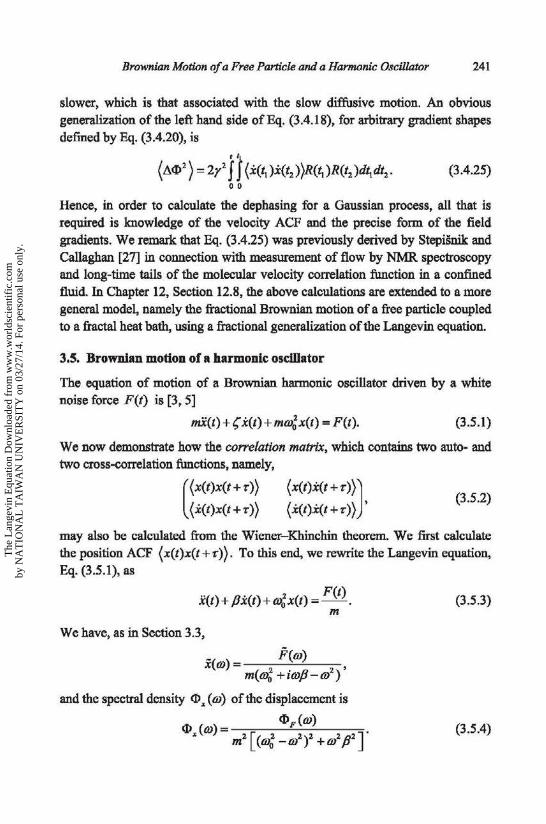
Brownian Motion of a Free Particle and a Harmonic Oscillator 241
slower, which is that associated with the slow diffusive motion. An obvious generalization of the left hand side ofEq. (3.4.18), for arbitrary gradient shapes defmed by Eq. (3.4.20), is
t t1
(A(f)2
) = 2y2 I I (x(t1)x(t2))R(tl)R(t2 )dtl dt2. (3.4.25)
0 0
Hence, in order to calculate the dephasing for a Gaussian process, all that is required is knowledge of the velocity ACF and the precise form of the field gradients. We remark that Eq. (3.4.25) was previously derived by StepiSnik and Callaghan [27] in connection with measurement of flow by NMR spectroscopy and long-time tails of the molecular velocity correlation function in a confined
fluid. In Chapter 12, Section 12.8, the above calculations are extended to a more general model, namely the fractional Brownian motion of a free particle coupled to a fractal heat bath, using a fractional generalization of the Langevin equation.
3.5. Brownian motion of a harmonic oscillator
The equation of motion of a Brownian harmonic oscillator driven by a white noise force F(t) is [3, 5]
mi(t) +; :X(t) + mm; x(t) = F(t). (3 .5 .1)
We now demonstrate how the correlation matrix, which contains two auto- and two cross-correlation functions, namely,
[
( x(t)x(t +1"))
(x(t)x(t+r)) (x(t):X(t+r))J·
(x(t)x(t+r)) (3.5.2)
may also be calculated from the Wiener-Khinchin theorem. We first calculate
the position ACF (x(t)x(t + 't')). To this end, we rewrite the Langevin equation, Eq. (3.5.1), as
x(t) + Px(t) +% x(t) = F(t). m
(3.5.3)
We have, as in Section 3.3,
i(m) = F(m) m(m~ +im,8-m2
)'
and the spectral density (f) x ( m) of the displacement is
(f) (m) = cD F (m) . x mz[(m;-mz)z+mzpz]
(3.5.4)
The
Lan
gevi
n E
quat
ion
Dow
nloa
ded
from
ww
w.w
orld
scie
ntif
ic.c
omby
NA
TIO
NA
L T
AIW
AN
UN
IVE
RSI
TY
on
03/2
7/14
. For
per
sona
l use
onl
y.
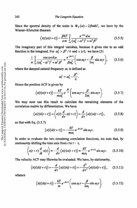
242 The Langevin Equation
Since the spectral density of the noise is <D F ( m) = 2 f3mkT, we have by the Wiener-Khinchin theorem
f3kT "" e-ttDT d m {x(t)x(t+t")) =--J 2 2 2 2 2 •
Km ....., (% - m ) + m p (3.5.5)
The imaginary part of this integral vanishes, because it gives rise to an odd function in the integrand. For % > {32 /4 and • ~ 0, we have [3]
1 "'s cos m-rdm e-ftTIZ ( f3 . ) - =-- cos~•+-sm~T, K ....., ( m; - m2
)2 + m2 {32 pm; 2~
where the damped natural frequency lVJ. is defined as
~2 = w; -p2 . 4
Hence the position ACF is given by
{x(t)x(t+-r)) =--2
e 2 cos~T+-sin~T . kT __!!!_ ( f3 ) mmo 2~
We may now use this result to calculate the remaining elements correlation matrix by differentiation. We have
(x(t)i(t+T)) = (x(t)~x(t+T)) =~(x(t)x(t+t")), dT dT
so that with Eq. (3.5.7)
(x(t)x(t+ -r)) =- kT e-PTtz sin ~-r. m~
(3.5.6)
(3.5.7)
of the
(3.5.8)
(3.5.9)
In order to evaluate the two remaining correlation functions, we note that, by stationarity shifting the time axis from t to t - t",
( x(t+ •)!!_x(t)) = -~(x(t)x(t+•)) = kT e- PT'2 sin ~T. (3.5.10) dt dT m~
The velocity ACF may likewise be evaluated. We have, by stationarity,
(x(t)x(t+ •>) = -~(x(t)x(t +T)) =- d2
2 (x(t)x(t+ •>), (3.5.11)
dt" dt"
whence
(3.5.12)
The
Lan
gevi
n E
quat
ion
Dow
nloa
ded
from
ww
w.w
orld
scie
ntif
ic.c
omby
NA
TIO
NA
L T
AIW
AN
UN
IVE
RSI
TY
on
03/2
7/14
. For
per
sona
l use
onl
y.

Brownian Motion of a Free Particle and a Harmonic Oscillator
The correlation matrix of the harmonic oscillator is thus
[~(cos~ T +_/!_sin~ T) kT -PT/2 liJQ 2~ -e m 1 .
-sm~T
~
--sm~T
1 . l co~~ T- _/!_sin OJT •
2~
243
(3.5.13)
Clearly, the under-damped process has significant memory of previous positions (cf. Fig. 1.3.1.1). Thus, x(t) is regarded as [3] the projection of the twodimensional Markov process {x(t),i(t)}.
3.6. Rotational Brownian motion of a fixed-His rotator
In his first model of the phenomenon of dielectric relaxation, given in 1913, Debye [12] considered a system of molecules each carrying a permanent dipole Jl, with every molecule free to rotate about a fixed axis (see Chapter 2, Section 2.6). Supposing that an external spatially uniform small d.c. electric field E ( q= pE I (kT) << 1) had been applied to the system at t = --«>, and at time t = 0 the
field has been switched off, the equation of motion of the fixed-axis rotator is
qO(t) + pE sin O(t) = A.(t), t ~ o, and qO(t) = A.(t), t > o, (3.6.1)
where O(t) is the angle between the dipole Jl and the direction the field E, and
A. (t) is a white-noise driving torque. One can then show that the PDF f(O, t) of the dipole moment orientations satisfies the Smoluchowski equation
of o2 f 'l"n-=-, t>O, (3.6.2)
at off where Tn = q I (kT) is the Debye relaxation time for rotation about a fixed axis. Equation (3 .6.2) together with the initial condition
1 ( pE ) /(0,0) = 2
7r 1+ kT cosO+··· (3.6.3)
then yields in the linear response approximation the well-known result [12] for
the mean dipole moment
(3.6.4)
Inertial effects are included by simply restoring the inertial term IB in Eq. (3.6.1) above. Thus, that equation becomes
IO(t) + qO(t)+ pE sin O(t) = A.(t) (3.6.5)
The
Lan
gevi
n E
quat
ion
Dow
nloa
ded
from
ww
w.w
orld
scie
ntif
ic.c
omby
NA
TIO
NA
L T
AIW
AN
UN
IVE
RSI
TY
on
03/2
7/14
. For
per
sona
l use
onl
y.

244 The Langevin Equation
fort<O, and
I B(t) + qO(t) = A.(t) (3.6.6)
for t>O. Equation (3.6.6) is a Langevin equation of the same form as that governing translational Brownian motion; see Eq. (3.2.3). Consequently, all the results we have previously obtained for the translational case can be applied to rotational Brownian motion. In particular, the mean-square angular displacement {(.110)2} is given by
{(.110)2} = 2k~ (Pt-l+e-Pr), IP
(3.6.7)
where p = ~ I I is the rotational damping coefficient. We note that, just as in all the other models treated in this Chapter, Eq. (3.6.6) comprises a linear stochastic differential equation with constant coefficients. This is of central importance to what follows, where a theorem about characteristic functions of Gaussian random variables [28] is used to calculate the dipole moment ACF.
Theorem about Gaussian random variables
The theorem is that, if X is a random variable with a Gaussian distribution, then [28]
(3.6.8)
(cf. Eq. (3.4.24); see also Chapter 1, Section 1.6.3). Consider now the ACF (cos0(t1)cos O(t2 )) = (cos0(t1)cos[O(t1)+AOD, where AO = 0(12 )-0(11 ). This
becomes, on expanding the terms within the angular brackets,
(cos O(t1) cos O(t2 )) = ~{ (cosAO) + (cos [ AO+ 20(t1) ])}
= ~Re[ (emiJ )+ (e;~e+2e<~>) J' (3.6.9)
where Re denotes "real part of." Now, if O{t1) and O(t2) are Gaussian random variables, any linear combination of them (e.g., AO) is also a Gaussian random variable. Hence
( ( ) ( )) 1 [ I(M)-![(CM)1)-(M)1
] cosO 11 cosO t2 =-Re e 2
2
+e1(~11+211(~>)-~ ([ ~~~+211(~m-<c ~~~+2tl(~lJ)'] J (3.6.10)
The
Lan
gevi
n E
quat
ion
Dow
nloa
ded
from
ww
w.w
orld
scie
ntif
ic.c
omby
NA
TIO
NA
L T
AIW
AN
UN
IVE
RSI
TY
on
03/2
7/14
. For
per
sona
l use
onl
y.

Brownian Motion of a Free Particle and a Harmonic Oscillator 245
Now, if the process we are considering is stationary, only those terms in Eq. (3.6.10) which are functions of the time difference I tz-tll will survive, so that Eq. (3.6.10) will take on the simple form
(cos 0 (t1 )cos O(t2 )) = (1 I 2)e -[(<Ml•)-(411)
1
]12
Re {ei(M)}. (3.6.11)
Further, if 0 is a centered Gaussian random variable (i.e., ( 0) = 0), then Eq. (3.6.11) reduces to
(cos 0 ( 11
) cos 0( 12 )) = (1 I 2)e -(<4
9)
2
)12
• (3.6.12)
Thus knowledge of ((1:10))2 is now sufficient to allow us to calculate averages. We have given the theorem for n = 1. For any integer value of n it is simply
(cos nO (t1
) cos nO(t2 )) = (1 I 2)e -,i'((t.llf)n. (3.6.13)
We reiterate that this equation is true only for centered Gaussian random variables. Thus the theorem will only hold good for those systems where 0 satisfies a linear differential equation of motion.
Application to dielectric relaxation
We may have, from Eq. (3.6.7) and (3.6.12), the ACF C(l):
~Pt-1+•-") C(t) = (cos 0(0) cos O(t)) J ( cos2 0(0)) = e rtf . (3.6.14)
The complex polarizability a is written down using the linear response formula, Chapter 2, Eq. (2.8.10). It is (with i(i)=s)
a(s) =1-sj e-'1C(t)dt. (3.6.15) a'(O) 0
Hence [7]
a(s) s [ r y2 J a'(O) =
1- s+rP
1+ (sl fJ)+r+1 + [(sl P)+r+1][(sl P)+r+2] + ...
ST0 [ ] =1---M 1,1+y(l+sr0 ),y, 1+sr0
(3.6.16)
where r =kT I(IP2) is Sack's inertial parameter [57], r 0 = 11(py), and
M(a,b,z) is the confluent hypergeometric (Kummer) function defined [29] as
M {a b z) = 1 +!:z+ a( a +I) z2 +a( a +I)( a+ 2) z3 + .. ·. (3.6.17) • • b b(b+1) 2! b(b+l)(b+2) 3!
The
Lan
gevi
n E
quat
ion
Dow
nloa
ded
from
ww
w.w
orld
scie
ntif
ic.c
omby
NA
TIO
NA
L T
AIW
AN
UN
IVE
RSI
TY
on
03/2
7/14
. For
per
sona
l use
onl
y.

246 The Langevin Equation
This result shows that the effect of including the inertia of the dipole is to produce a denumerable set of relaxation mechanisms. The series in Eq. (3.6.16) may be rewritten as the continued fraction [7, 8]
a(s) =l- sf p a'(O) Y
sf P+ 2 l+sf P+ r
2+sf P+ 3Y
3+sf P+···
(3.6.18)
The first convergent ofEq. (3 .6.18) yields the De bye relaxation formula
a(s) =-1-a'(O) 1 + St"n
(3.6.19)
The second convergent ofEq. (3.6.18) yields the Rocard equation [30]
a(s) rP2 _ 1
a'(O) (s + rP)(s + p) = 1 + s-r0 + s 2-rn I p · (3.6.20)
This provides [7] a good approximation to the relaxation behavior, provided that r~ 0.05. Equations (3.6.16) and (3.6.20) have been exhaustively discussed in Chapter 2 of Molecular Dynamics [10]. It is evident that the simple Debye model, including an inertial correction, is not sufficient to explain the experimental evidence. The inertial correction embodied in Eq. (3.6.20) does, however, remove the unacceptable plateau in the high-frequency absorption profile (see Section 1.15.1). The same holds true for all the three-dimensional versions of the Debye model, including inertial effects. These are the sphere, prolate and oblate spheroid, and general ellipsoid The far-infrared absorption
and the microwave absorption linked to it cannot be satisfactorily explained by the Debye theory with inertial corrections only.
As a prelude to the itinerant oscillator model of Chapter 11, which is an attempt to address the Poley absorption theoretically, we now treat the torsional oscillator model, originally discussed by Calderwood et al. [9].
3.7. Torsional oscillator model: example of the use of the Wiener integral
The simplest model that takes any account of the effect of the neighbors of a molecule on its relaxation behavior is where we regard the molecule as a torsional oscillator. Thus, we suppose that at a time t after the switching off of a field which had been steady up to t = 0, the equation of motion of the dipole is
O(t)+ pli(t)+ %O(t) = W(t), (3.7.1)
The
Lan
gevi
n E
quat
ion
Dow
nloa
ded
from
ww
w.w
orld
scie
ntif
ic.c
omby
NA
TIO
NA
L T
AIW
AN
UN
IVE
RSI
TY
on
03/2
7/14
. For
per
sona
l use
onl
y.
Brownian Motion of a Free Particle and a Harmonic Oscillator 247
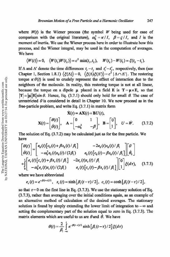
where W(t) is the Wiener process (the symbol W being used for ease of comparison with the original literature), CO: = K I I, P =!:I I, and I is the moment of inertia. We use the Wiener process here in order to illustrate how this process, and the Wiener integral, may be used in the computation of averages. We have
{W(t)) = 0, {W(t1 )W(t2 )) = c2 min(t1, t2 ), W(t2 )-W(t1 ) = ~(t2 - t1 ).
If!!.. and fl.' denote the time differences t; -ti and t; -t;, respectively, then (see Chapter 1, Section 1.8.1) (~(!!..))=0, (~(fl.)~(fl.'))=c2 1 fl.nfl.'l· The restoring torque K 8(t) is used to crudely represent the effect of interaction due to the neighbors of the molecule. In reality, this restoring torque is not at all linear, because the torque on a dipole 11. placed in a field E is T = I' x E, so that ITI=IJ&IIEisinO. Hence, Eq. (3.7.1) should only hold for small 0. The case of unrestricted 0 is considered in detail in Chapter 10. We now proceed as in the free-particle problem, and write Eq. (3. 7.1) in matrix form
X(t) = AX(t) + BU(t),
X(t)=[~(t)]• A=[O 2 I ]• B=[0], U=W. (3.7.2)
O(t) -roo -P I
The solution ofEq. (3.7.2) may be calculated just as for the free particle. We have
[O(t)] [e0 (t) [ c0 (t) + Ps0 (t) I f3.] - 2ea (t)so (t) I A. l [(} ] O(t) - - m; ea (t)so (t) I (2fit) eo (t) [Co (t)- Pso (t) I PI] Oo
1 [e, (t) [ c, (t) + Ps, (t) I fit] -2e, (t)s, (t) I P1 l [OJ +J ~(d-r), 0 - m; e, (t)s, (t) I (2P1) e, (t) [ c, (t)- Ps, (t) I fit] 1
(3.7.3)
where we have abbreviated
e, (t) = e-P(H)Iz, sr (t) =sinh [P1 (t- -r) I 2], c, (t) =cosh (P1 (t- -r) I 2],
so that -r= 0 on the first line in Eq. (3.7.3). We use the stationary solution ofEq. (3.7.3), rather than averaging over the initial conditions again, as an example of an alternative method of calculation of the desired averages. The stationary solution is found by simply extending the lower limit of integration to - oo and
setting the complementary part of the solution equal to zero in Eq. (3.7.3). The matrix elements which are useful to us are 0 and iJ. We have
O(t) = ~ l e-PCt-•l'2 sinh (P1 (t--r) I 2] ~(d-r)
The
Lan
gevi
n E
quat
ion
Dow
nloa
ded
from
ww
w.w
orld
scie
ntif
ic.c
omby
NA
TIO
NA
L T
AIW
AN
UN
IVE
RSI
TY
on
03/2
7/14
. For
per
sona
l use
onl
y.

248 The Langevin Equation
and thus I
B(t) = J e-P<~-<>'2 (cosh [A (t --r) I 2]- (/3 I P1 ) sinh [P1 (t--r) I 2])t;(d-r),
where A2 = ft2
- 4m;. The formulas appropriate for the periodic (./3! is imaginary) and the critically damped (./3! = 0) cases can be written down by replacing P1-
1 sinh(A t I 2) and cosh(A t I 2), respectively, by (2Wt f 1 sin Wt t and cos 01 t, in the periodic case, and by 1 and t I 2 in the critically damped case.
We now define a function
{(21 A)e-P<~-<>'2 sinh[P: (t--r)l2], -r !.t,
g,(T)= 0 I , T>t
Thus by the properties of the Wiener integral,
"' (O(t1 ) O(t2 )) = c2 J g~ (-r)gr. (-r)d-r
- 4c2 min(Jt,.t.) -1<~-r) inh [A { )] -~(r.-r) inh [A { )] d -- e S - t -T e S - t -T T Az....., 21 22
= 2;~ (cosh[~ (t2 -t,)]+ ~sinh(~ lt2 -t1 1)}~"-"1 • Similarly, one may deduce that
(8(tt)B(t2 )) = ;~ ( cosh[A (t2 -tt)l 2]-~ sinh [P, lt2 -t1 l I 2 J }-Pir.-~tl/2
and that (O(t1 )) = \O(t2 )) = 0. Thus, for equal times, t. = t2 = t say, we have ( 02 (t)) = c2 I (2ftw0 ) and ( 02 (t)) = c_2 I (2ft). If we assume. the Maxwellian distribution for the angular velocity O(t), we must have I ( 02 (t)) I 2 = kT I 2 and thus c2 I (2ft)= kT I I. From this, with t1 = 0, t2 = t, we have
{O(O)O(t)) = kT2
[cosh(/31t I 2)+f!_sinh(ft1t I 2)] e-P''2
Imo P1 and (02 (0)) = (02 (t)) = kT I (I w;). Substituting from all these equations into
Eq. (3.6.10), we find that [9]
(cosO(O)cos O(t)) = e-r cosh{re-11'12 [ cosh(At I 2)+(P I ft1)sinh(At I 2)]},
where, in this instance, r = kT I (I w;). Note that Eq. (3.6.10) must be used
rather than Eq. (3.6.13), because the second term on the right of Eq. (3.6.10) does not now vanish, as a result of the influence of the restoring torque.
The
Lan
gevi
n E
quat
ion
Dow
nloa
ded
from
ww
w.w
orld
scie
ntif
ic.c
omby
NA
TIO
NA
L T
AIW
AN
UN
IVE
RSI
TY
on
03/2
7/14
. For
per
sona
l use
onl
y.
Brownian Motion of a Free Particle and a Harmonic Oscillator 249
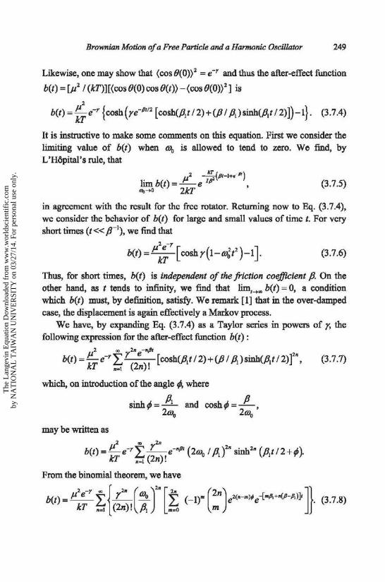
Likewise, one may show that (cos 0(0))2 = e-r and thus the after-effect function
b(t) = [.ti I (kT)] [ (cos 0(0) cos O(t)) - (cos O(O)) 2 ] is
2
b(t) = Zr e-r {cosh (re-P112 [ cosh(JV I 2) +{PI P1) sinh(At I 2)])- t}. (3.7.4)
It is instructive to make some comments on this equation. First we consider the limiting value of b(t) when lDo is allowed to tend to zero. We find, by L'Hapital's rule, that
(3.7.5)
in agreement with the result for the free rotator. Returning now to Eq. (3.7.4), we consider the behavior of b(t) for large and small values of time t. For very short times (t<< p-1
), we find that 2 -r
b(t) = P; [ coshr(t-%t2 )-1]. (3.7.6)
Thus, for short times, b(t) is independent of the friction coefficient p. On the other hand, as t tends to infinity, we find that lim~-+., b(t) = 0, a condition which b(t) must, by defmition, satisfY. We remark [1] that in the over-damped case, the displacement is again effectively a Markov process.
We have, by expanding Eq. (3.7.4) as a Taylor series in powers of y, the following expression for the after-effect function b(t):
2 ., 2n -•fJt
b(t) =Le-rL r e [cosh(plt 12)+(11 I Pt)sinh(At 12)t'' (3.7.7) kT n~l (2n)!
which, on introduction of the angle ;, where
sinh; = A and cosh; = __!!_, 2t.V0 2cv0
may be written as 2 ., 2n
b(t) =Le-rL_r_e-•flt (2t.V0 I P1t sinh2" (P1t 12+;).
kT n=l (2n)!
From the binomial theorem, we have
b(t)= p2e-r i:{ r2• ,(%)2" [t (-1)"' (2n)e2(n-m);e-[mPt+•{P-Pt)]t]}· (3.7.8) kT • =l (2n). Pt m=O m
The
Lan
gevi
n E
quat
ion
Dow
nloa
ded
from
ww
w.w
orld
scie
ntif
ic.c
omby
NA
TIO
NA
L T
AIW
AN
UN
IVE
RSI
TY
on
03/2
7/14
. For
per
sona
l use
onl
y.

250 The Langevin Equation
We now recall that the complex polarizability a(w) is defined by Eq. (2.8.9) of Chapter 2. From this, with Eq. (3.7.8), we have
2 e -r "' y2n (% J2
n [ 2n m (2nJ e2<n-m); l
a(co)=f.J -L- - L(-1) . kT n=l (2n)! P, -o m l+ian-.,,.
(3.7.9)
Here r~:n =m/31 +n(P-A.). The factor in square brackets in Eq. (3.7.9) represents the partial-fraction expansion of the Fourier transform of
e-n{Jt sinh2n (/J,.t/2+;).
One may calculate successive terms in Eq. (3.7.9) by expanding the expression in square brackets in that equation for n = 1, 2, 3, .... Thus for n = 1, the value of this expression is
(p + ico)[(p + ico)2 - /3,.2 ] '
while for n = 2 we must add the term
(3.7.10)
4 /3,.4
{{2/3 +ico)3 + 3/3(2/3 +ico)
2 + 2(5% + /32 )(2/3 + iw) + 12% /3}·
% (2P + iw)[(2f3 + iw)2 - /3,.2 ][(2P + iw)2 -413,.2 ]
Clearly, the polarizability in the under-damped case w; > /32 /4 consists of a discrete set of resonant absorptions [31]. This is of importance in connection with the itinerant oscillator model, which has been extensively used to discuss the far-infrared (Poley) absorption [10, 31]; we describe this in Chapter 11 (see also Chapter 10, Section 10.4.3).
References
1. P. Langevin (1908). Sur la tbeorie de mouvement brownien, C. R. Acad. Sci. Paris, 146, 530. (English translation: P. Langevin (1997). On the theory of Brownian motion, Am. J. Phys., 65, 1079.)
2. G.E. Uhlenbeck and L.S. Ornstein (1930). On the theory of the Brownian motion, Phys. Rev., 36,823.
3. M.C. Wang and G.E. Uhlenbeck (1945). On the theory of the Brownian motion II, Rev. Mod. Phys., 17, 323.
4. A. Einstein (1954). Investigations on the theory of the Brownian movement, Dover, New York.
5. M. Gitterman (2005). The Brownian Oscillator, World Scientific, Singapore. 6. R. Zwanzig (2001). Nonequilibrium Statistical Mechanics, Oxford University Press,
Oxford. 7. R.A. Sack (1957). Relaxation processes and inertial effects 1: Free rotation about a
fixed axis, Proc. Phys. Soc. B, 70, 402.
The
Lan
gevi
n E
quat
ion
Dow
nloa
ded
from
ww
w.w
orld
scie
ntif
ic.c
omby
NA
TIO
NA
L T
AIW
AN
UN
IVE
RSI
TY
on
03/2
7/14
. For
per
sona
l use
onl
y.

Brownian Motion of a Free Particle and a Harmonic Oscillator 251
8. E.P. Gross (1955). Inertial effects and dielectric relaxation, J. Chem. Phys., 23, 1415. 9. J.H. Calderwood, W.T. Coffey, A. Morita, et al. (1976). A model for the frequency
dependence of the polarizability of a polar molecule, Proc. R. Soc. Lond. A, 352, 275. 10. M.W. Evans, G.J. Evans, W.T. Coffey, et al. (1982). Molecular Dynamics, Wiley
lnterscience, New York. 11. N. Gershenfeld (2000). The Physics of Information Technology, Cambridge
University Press, Cambridge, UK. 12. P. Debye (1929). Polar Molecules, Chemical Catalog, New York (reprinted by Dover
publications, New York, 1954). 13. J.L. Doob (1942). The Brownian movement and stochastic equations, Ann. Math., 43,
351. 14. J.A. Aseltine (1958). Transform Method in Linear System Analysis, McGraw-Hill,
New York. 15. L. Van Hove (1954). Correlations in space and time and Born approximation
scattering in systems of interacting particles, Phys. Rev., 95,249. 16. G.H. Vineyard (1958). Scattering of slow neutrons by a liquid, Phys. Rev., 110, 999. 17. D.M. K.oh and H.C. Thoeny, Eds. (2010). Diffusion-Weighted MR. Imaging, Springer,
Berlin. 18. F. Bloch (1946). Nuclear induction, Phys. Rev., 70, 460. 19. E.L. Hahn (1950). Spin echoes, Phys. Rev., 80,580. 20. T.P. Das and A.K. Saha (1954). Mathematical analysis of the Hahn spin echo
experiment, Phys. Rev., 93, 749. 21. H.Y. Carr and E.M. Purcell (1954). Effects of diffusion on free precession in nuclear
magnetic resonance experiments, Phys. Rev., 94, 630. 22. M. Kac (1947). Random walk and the theory of Brownian motion. Am. Math. Mon.,
54, 369. Reprinted inN. Wax, Ed. (1954). Selected Papers on Noise and Stochastic Processes, Dover, New York.
23. H.C. Torrey (1956). The Bloch equation with diffusion terms, Phys. Rev., 104, 563. 24. A. Abragam. (1961). The Principles of Nuclear Magnetism, Oxford University Press,
London. 25. D.S. Grebenkov (2007). NMR survey of reflected Brownian motion, Rev. Mod.
Phys., 19, 1077. 26. E.O. Stejskal and J.E. Tanner (1965). Spin diffusion measurements: Spin echoes in
the presence of a time-dependent field gradient, J. Chem. Phys., 42, 288. 27. J. Stepisnik. and P.T. Callaghan (2000). The long time tail of molecular velocity
correlation in a confined fluid: Observation by modulated gradient spin-echo NMR. Physica B, 292, 296; J. Stepi~nik. (1993). Time-dependent self-diffusion by NMR spin-echo, Physica B, 183, 343.
28. H. Cram.6r (1970). Random Variables and Probability Distributions, Cambridge Tracts on Mathematics and Mathematical Physics, No. 36, Cambridge University Press, Cambridge, UK.
29. M. Abramowitz and I. Stegun, Eds. (1964). Handbook of Mathematical Functions, Dover, New York.
The
Lan
gevi
n E
quat
ion
Dow
nloa
ded
from
ww
w.w
orld
scie
ntif
ic.c
omby
NA
TIO
NA
L T
AIW
AN
UN
IVE
RSI
TY
on
03/2
7/14
. For
per
sona
l use
onl
y.

252 The Langevin Equation
30. M.Y. Rocard (1933). Analyse des orientations m.olecuJ.aires de molecules a moment permanent dans un champ altematif. Application a la dispersion de Ia constante dielectrique eta l'effet Kerr, J. Phys. Radium, 4, 247.
31. W.T. Coffey, P.M. Corcoran, and M.W. Evans (1987). On the role of inertial effects and dipole-dipole coupling in the theory of the Debye and far-infrared absorption of polar fluids, Proc. R. Soc. Lond. A, 410, 61.
The
Lan
gevi
n E
quat
ion
Dow
nloa
ded
from
ww
w.w
orld
scie
ntif
ic.c
omby
NA
TIO
NA
L T
AIW
AN
UN
IVE
RSI
TY
on
03/2
7/14
. For
per
sona
l use
onl
y.