A SHIFTED BLOCK LANCZOS ALGORITHM FOR SOLVING SPARSE SYMMETRIC GENERALIZED EIGENPROBLEMS
The Lanczos and conjugate gradient algorithms
Gerard MEURANT
October, 2008
1 The Lanczos algorithm
2 The Lanczos algorithm in finite precision
3 The nonsymmetric Lanczos algorithm
4 The Golub–Kahan bidiagonalization algorithm
5 The block Lanczos algorithm
6 The conjugate gradient algorithm
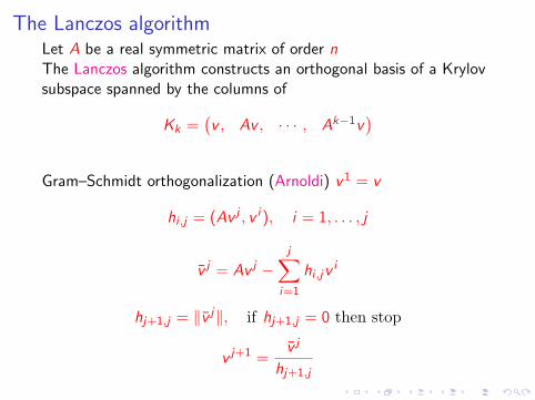
The Lanczos algorithmLet A be a real symmetric matrix of order nThe Lanczos algorithm constructs an orthogonal basis of a Krylovsubspace spanned by the columns of
Kk =(v , Av , · · · , Ak−1v
)Gram–Schmidt orthogonalization (Arnoldi) v1 = v
hi ,j = (Av j , v i ), i = 1, . . . , j
v j = Av j −j∑
i=1
hi ,jvi
hj+1,j = ‖v j‖, if hj+1,j = 0 then stop
v j+1 =v j
hj+1,j
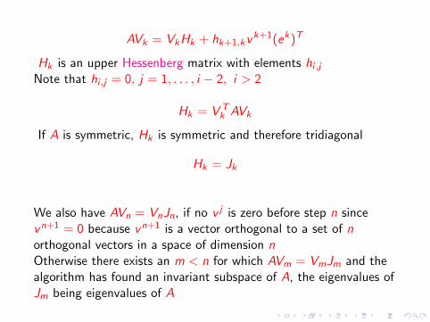
AVk = VkHk + hk+1,kvk+1(ek)T
Hk is an upper Hessenberg matrix with elements hi ,j
Note that hi ,j = 0, j = 1, . . . , i − 2, i > 2
Hk = V Tk AVk
If A is symmetric, Hk is symmetric and therefore tridiagonal
Hk = Jk
We also have AVn = VnJn, if no v j is zero before step n sincevn+1 = 0 because vn+1 is a vector orthogonal to a set of northogonal vectors in a space of dimension nOtherwise there exists an m < n for which AVm = VmJm and thealgorithm has found an invariant subspace of A, the eigenvalues ofJm being eigenvalues of A
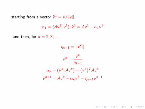
starting from a vector v1 = v/‖v‖
α1 = (Av1, v1), v2 = Av1 − α1v1
and then, for k = 2, 3, . . .
ηk−1 = ‖vk‖
vk =vk
ηk−1
αk = (vk ,Avk) = (vk)TAvk
vk+1 = Avk − αkvk − ηk−1vk−1
A variant of the Lanczos algorithm has been proposed byChris Paige to improve the local orthogonality in finite precisioncomputations
αk = (vk)T (Avk − ηk−1vk−1)
vk+1 = (Avk − ηk−1vk−1)− αkvk
Since we can suppose that ηi 6= 0, the tridiagonal Jacobi matrix Jk
has real and simple eigenvalues which we denote by θ(k)j
They are known as the Ritz values and are the approximations ofthe eigenvalues of A given by the Lanczos algorithm
TheoremLet χk(λ) be the determinant of Jk − λI (which is a monicpolynomial), then
vk = pk(A)v1, pk(λ) = (−1)k−1 χk−1(λ)
η1 · · · ηk−1
The polynomials pk of degree k − 1 are called the normalizedLanczos polynomials
The polynomials pk satisfy a scalar three–term recurrence
ηkpk+1(λ) = (λ− αk)pk(λ)− ηk−1pk−1(λ), k = 1, 2, . . .
with initial conditions, p0 ≡ 0, p1 ≡ 1
TheoremConsider the Lanczos vectors vk . There exists a measure α suchthat
(vk , v l) = 〈pk , pl〉 =
∫ b
apk(λ)pl(λ)dα(λ)
where a ≤ λ1 = λmin and b ≥ λn = λmax , λmin and λmax beingthe smallest and largest eigenvalues of A
Proof.Let A = QΛQT be the spectral decomposition of ASince the vectors v j are orthonormal and pk(A) = Qpk(Λ)QT , wehave
(vk , v l) = (v1)Tpk(A)Tpl(A)v1
= (v1)TQpk(Λ)QTQpl(Λ)QT v1
= (v1)TQpk(Λ)pl(Λ)QT v1
=n∑
j=1
pk(λj)pl(λj)[vj ]2,
where v = QT v1
The last sum can be written as an integral for a measure α whichis piecewise constant
α(λ) =
0 if λ < λ1∑i
j=1[vj ]2 if λi ≤ λ < λi+1∑n
j=1[vj ]2 if λn ≤ λ
The measure α has a finite number of points of increase at the(unknown) eigenvalues of A
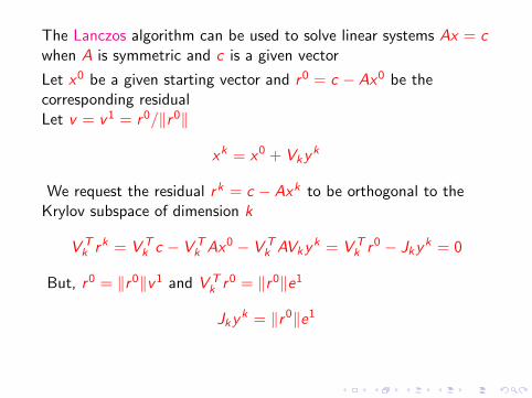
The Lanczos algorithm can be used to solve linear systems Ax = cwhen A is symmetric and c is a given vector
Let x0 be a given starting vector and r0 = c − Ax0 be thecorresponding residualLet v = v1 = r0/‖r0‖
xk = x0 + Vkyk
We request the residual rk = c − Axk to be orthogonal to theKrylov subspace of dimension k
V Tk rk = V T
k c − V Tk Ax0 − V T
k AVkyk = V Tk r0 − Jkyk = 0
But, r0 = ‖r0‖v1 and V Tk r0 = ‖r0‖e1
Jkyk = ‖r0‖e1
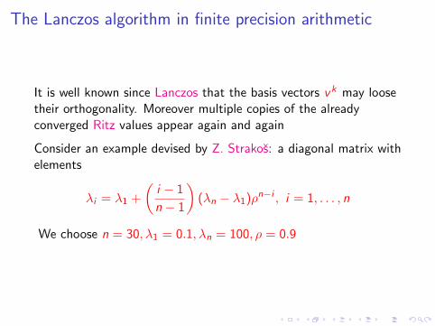
The Lanczos algorithm in finite precision arithmetic
It is well known since Lanczos that the basis vectors vk may loosetheir orthogonality. Moreover multiple copies of the alreadyconverged Ritz values appear again and again
Consider an example devised by Z. Strakos: a diagonal matrix withelements
λi = λ1 +
(i − 1
n − 1
)(λn − λ1)ρ
n−i , i = 1, . . . , n
We choose n = 30, λ1 = 0.1, λn = 100, ρ = 0.9
05
1015
2025
30
0
5
10
15
20
25
30−20
−15
−10
−5
0
5
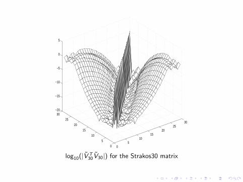
log10(|V T30V30|) for the Strakos30 matrix
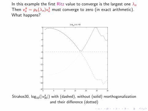
In this example the first Ritz value to converge is the largest one λn
Then vkn = pk(λn)v
1n must converge to zero (in exact arithmetic).
What happens?
0 5 10 15 20 25 30−20
−18
−16
−14
−12
−10
−8
−6
−4
−2
0
|Log10
∆ v|, i=30
Strakos30, log10(|vk30|) with (dashed), without (solid) reorthogonalization
and their difference (dotted)
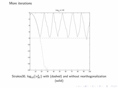
More iterations
10 20 30 40 50 60 70 80 90 100−18
−16
−14
−12
−10
−8
−6
−4
−2
0
|Log10
v|, i=30
Strakos30, log10(|vk30|) with (dashed) and without reorthogonalization
(solid)
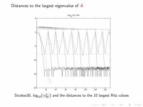
Distances to the largest eigenvalue of A
20 40 60 80 100 120 140−20
−15
−10
−5
0
5
|Log10
∆ v|, i=30
Strakos30, log10(|vk30|) and the distances to the 10 largest Ritz values
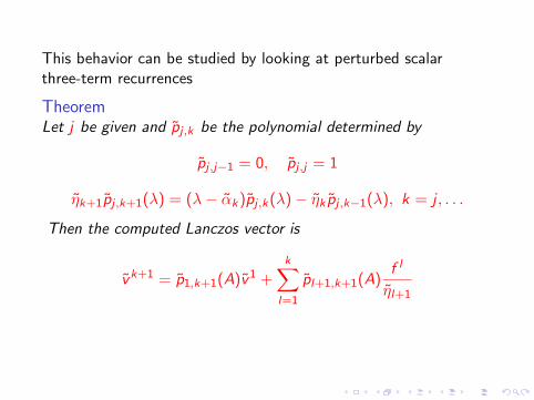
This behavior can be studied by looking at perturbed scalarthree-term recurrences
TheoremLet j be given and pj ,k be the polynomial determined by
pj ,j−1 = 0, pj ,j = 1
ηk+1pj ,k+1(λ) = (λ− αk)pj ,k(λ)− ηk pj ,k−1(λ), k = j , . . .
Then the computed Lanczos vector is
vk+1 = p1,k+1(A)v1 +k∑
l=1
pl+1,k+1(A)f l
ηl+1
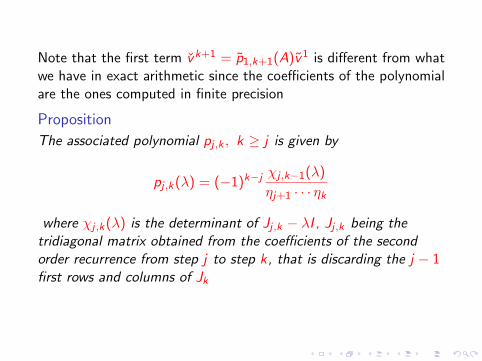
Note that the first term vk+1 = p1,k+1(A)v1 is different from whatwe have in exact arithmetic since the coefficients of the polynomialare the ones computed in finite precision
Proposition
The associated polynomial pj ,k , k ≥ j is given by
pj ,k(λ) = (−1)k−j χj ,k−1(λ)
ηj+1 · · · ηk
where χj ,k(λ) is the determinant of Jj ,k − λI , Jj ,k being thetridiagonal matrix obtained from the coefficients of the secondorder recurrence from step j to step k, that is discarding the j − 1first rows and columns of Jk
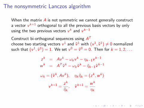
The nonsymmetric Lanczos algorithm
When the matrix A is not symmetric we cannot generally constructa vector vk+1 orthogonal to all the previous basis vectors by onlyusing the two previous vectors vk and vk−1
Construct bi-orthogonal sequences using AT
choose two starting vectors v1 and v1 with (v1, v1) 6= 0 normalizedsuch that (v1, v1) = 1. We set v0 = v0 = 0. Then for k = 1, 2, . . .
zk = Avk − ωkvk − ηk−1vk−1
wk = AT vk − ωk vk − ηk−1vk−1
ωk = (vk ,Avk), ηk ηk = (zk ,wk)
vk+1 =zk
ηk, vk+1 =
wk
ηk
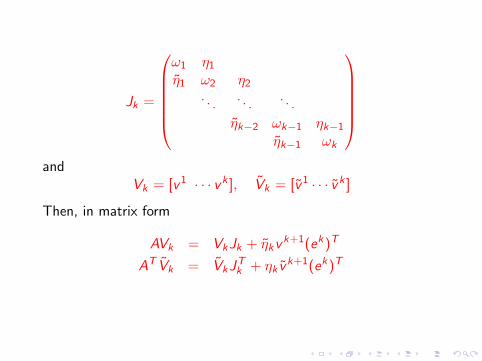
Jk =
ω1 η1
η1 ω2 η2
. . .. . .
. . .
ηk−2 ωk−1 ηk−1
ηk−1 ωk
and
Vk = [v1 · · · vk ], Vk = [v1 · · · vk ]
Then, in matrix form
AVk = VkJk + ηkvk+1(ek)T
AT Vk = VkJTk + ηk vk+1(ek)T
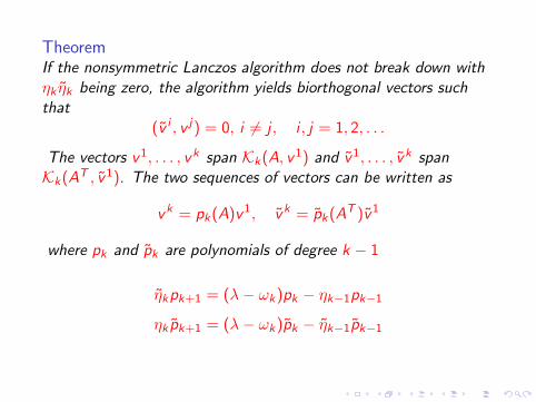
TheoremIf the nonsymmetric Lanczos algorithm does not break down withηk ηk being zero, the algorithm yields biorthogonal vectors suchthat
(v i , v j) = 0, i 6= j , i , j = 1, 2, . . .
The vectors v1, . . . , vk span Kk(A, v1) and v1, . . . , vk spanKk(AT , v1). The two sequences of vectors can be written as
vk = pk(A)v1, vk = pk(AT )v1
where pk and pk are polynomials of degree k − 1
ηkpk+1 = (λ− ωk)pk − ηk−1pk−1
ηk pk+1 = (λ− ωk)pk − ηk−1pk−1
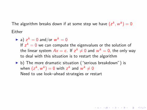
The algorithm breaks down if at some step we have (zk ,wk) = 0
Either
I a) zk = 0 and/or wk = 0If zk = 0 we can compute the eigenvalues or the solution ofthe linear system Ax = c . If zk 6= 0 and wk = 0, the only wayto deal with this situation is to restart the algorithm
I b) The more dramatic situation (“serious breakdown”) iswhen (zk ,wk) = 0 with zk and wk 6= 0Need to use look–ahead strategies or restart
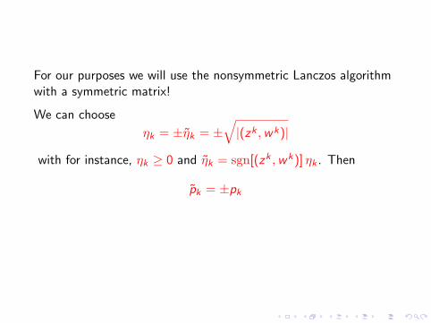
For our purposes we will use the nonsymmetric Lanczos algorithmwith a symmetric matrix!
We can choose
ηk = ±ηk = ±√|(zk ,wk)|
with for instance, ηk ≥ 0 and ηk = sgn[(zk ,wk)] ηk . Then
pk = ±pk
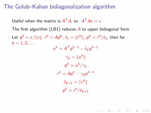
The Golub–Kahan bidiagonalization algorithm
Useful when the matrix is ATA, ex. ATAx = c
The first algorithm (LB1) reduces A to upper bidiagonal form
Let q0 = c/‖c‖, r0 = Aq0, δ1 = ‖r0‖, p0 = r0/δ1, then fork = 1, 2, . . .
uk = ATpk−1 − δkqk−1
γk = ‖uk‖
qk = uk/γk
rk = Aqk − γkpk−1
δk+1 = ‖rk‖
pk = rk/δk+1
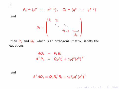
IfPk =
(p0 · · · pk−1
), Qk =
(q0 · · · qk−1
)and
Bk =
δ1 γ1
. . .. . .
δk−1 γk−1
δk
then Pk and Qk , which is an orthogonal matrix, satisfy the
equations
AQk = PkBk
ATPk = QkBTk + γkqk(ek)T
andATAQk = QkBT
k Bk + γkδkqk(ek)T
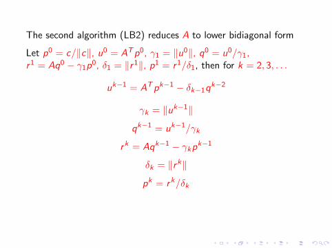
The second algorithm (LB2) reduces A to lower bidiagonal form
Let p0 = c/‖c‖, u0 = ATp0, γ1 = ‖u0‖, q0 = u0/γ1,r1 = Aq0 − γ1p
0, δ1 = ‖r1‖, p1 = r1/δ1, then for k = 2, 3, . . .
uk−1 = ATpk−1 − δk−1qk−2
γk = ‖uk−1‖
qk−1 = uk−1/γk
rk = Aqk−1 − γkpk−1
δk = ‖rk‖
pk = rk/δk
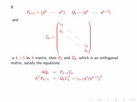
IfPk+1 =
(p0 · · · pk
), Qk =
(q0 · · · qk−1
)and
Ck =
γ1
δ1. . .. . .
. . .
. . . γk
δk
a k + 1 by k matrix, then Pk and Qk , which is an orthogonal
matrix, satisfy the equations
AQk = Pk+1Ck
ATPk+1 = QkCTk + γk+1q
k(ek+1)T
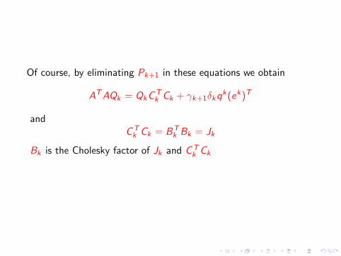
Of course, by eliminating Pk+1 in these equations we obtain
ATAQk = QkCTk Ck + γk+1δkqk(ek)T
andCT
k Ck = BTk Bk = Jk
Bk is the Cholesky factor of Jk and CTk Ck
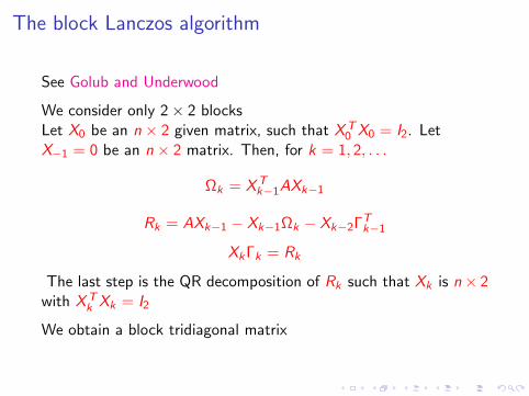
The block Lanczos algorithm
See Golub and Underwood
We consider only 2× 2 blocksLet X0 be an n × 2 given matrix, such that XT
0 X0 = I2. LetX−1 = 0 be an n × 2 matrix. Then, for k = 1, 2, . . .
Ωk = XTk−1AXk−1
Rk = AXk−1 − Xk−1Ωk − Xk−2ΓTk−1
XkΓk = Rk
The last step is the QR decomposition of Rk such that Xk is n× 2with XT
k Xk = I2
We obtain a block tridiagonal matrix
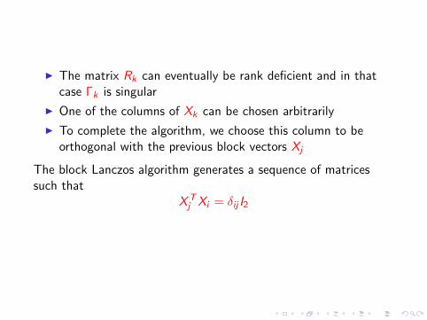
I The matrix Rk can eventually be rank deficient and in thatcase Γk is singular
I One of the columns of Xk can be chosen arbitrarily
I To complete the algorithm, we choose this column to beorthogonal with the previous block vectors Xj
The block Lanczos algorithm generates a sequence of matricessuch that
XTj Xi = δij I2
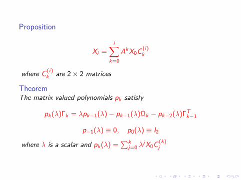
Proposition
Xi =i∑
k=0
AkX0C(i)k
where C(i)k are 2× 2 matrices
TheoremThe matrix valued polynomials pk satisfy
pk(λ)Γk = λpk−1(λ)− pk−1(λ)Ωk − pk−2(λ)ΓTk−1
p−1(λ) ≡ 0, p0(λ) ≡ I2
where λ is a scalar and pk(λ) =∑k
j=0 λjX0C(k)j
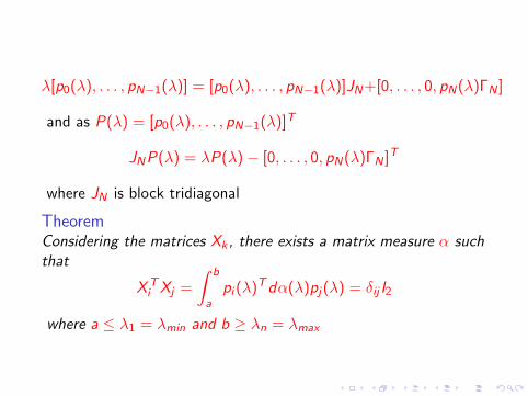
λ[p0(λ), . . . , pN−1(λ)] = [p0(λ), . . . , pN−1(λ)]JN+[0, . . . , 0, pN(λ)ΓN ]
and as P(λ) = [p0(λ), . . . , pN−1(λ)]T
JNP(λ) = λP(λ)− [0, . . . , 0, pN(λ)ΓN ]T
where JN is block tridiagonal
TheoremConsidering the matrices Xk , there exists a matrix measure α suchthat
XTi Xj =
∫ b
api (λ)Tdα(λ)pj(λ) = δij I2
where a ≤ λ1 = λmin and b ≥ λn = λmax
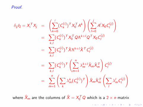
Proof.
δij I2 = XTi Xj =
(i∑
k=0
(C(i)k )TXT
0 Ak
)(j∑
l=0
AlX0C(j)l
)=
∑k,l
(C(i)k )TXT
0 QΛk+lQTX0C(j)l
=∑k,l
(C(i)k )T XΛk+l XTC
(j)l
=∑k,l
(C(i)k )T
(n∑
m=1
λk+lm XmXT
m
)C
(j)l
=n∑
m=1
(∑k
λkm(C
(i)k )T
)XmXT
m
(∑l
λlmC
(j)l
)
where Xm are the columns of X = XT0 Q which is a 2× n matrix
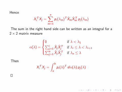
Hence
XTi Xj =
n∑m=1
pi (λm)T XmXTm pj(λm)
The sum in the right hand side can be written as an integral for a2× 2 matrix measure
α(λ) =
0 if λ < λ1∑i
j=1 Xj XTj if λi ≤ λ < λi+1∑n
j=1 Xj XTj if λn ≤ λ
Then
XTi Xj =
∫ b
api (λ)T dα(λ) pj(λ)
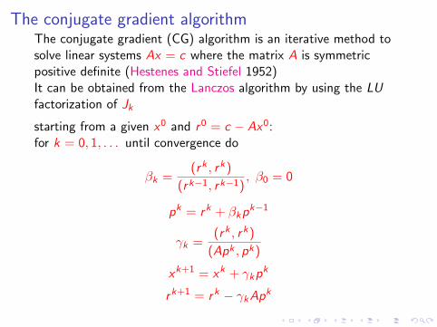
The conjugate gradient algorithmThe conjugate gradient (CG) algorithm is an iterative method tosolve linear systems Ax = c where the matrix A is symmetricpositive definite (Hestenes and Stiefel 1952)It can be obtained from the Lanczos algorithm by using the LUfactorization of Jk
starting from a given x0 and r0 = c − Ax0:for k = 0, 1, . . . until convergence do
βk =(rk , rk)
(rk−1, rk−1), β0 = 0
pk = rk + βkpk−1
γk =(rk , rk)
(Apk , pk)
xk+1 = xk + γkpk
rk+1 = rk − γkApk
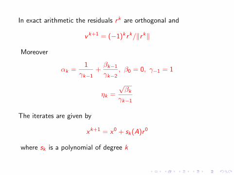
In exact arithmetic the residuals rk are orthogonal and
vk+1 = (−1)k rk/‖rk‖
Moreover
αk =1
γk−1+
βk−1
γk−2, β0 = 0, γ−1 = 1
ηk =
√βk
γk−1
The iterates are given by
xk+1 = x0 + sk(A)r0
where sk is a polynomial of degree k
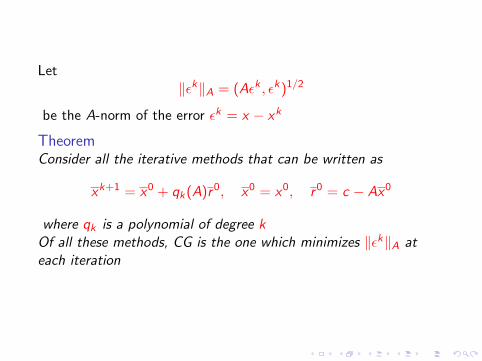
Let‖εk‖A = (Aεk , εk)1/2
be the A-norm of the error εk = x − xk
TheoremConsider all the iterative methods that can be written as
xk+1 = x0 + qk(A)r0, x0 = x0, r0 = c − Ax0
where qk is a polynomial of degree kOf all these methods, CG is the one which minimizes ‖εk‖A ateach iteration
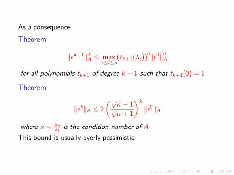
As a consequence
Theorem
‖εk+1‖2A ≤ max
1≤i≤n(tk+1(λi ))
2‖ε0‖2A
for all polynomials tk+1 of degree k + 1 such that tk+1(0) = 1
Theorem
‖εk‖A ≤ 2
(√κ− 1√κ + 1
)k
‖ε0‖A
where κ = λnλ1
is the condition number of A
This bound is usually overly pessimistic
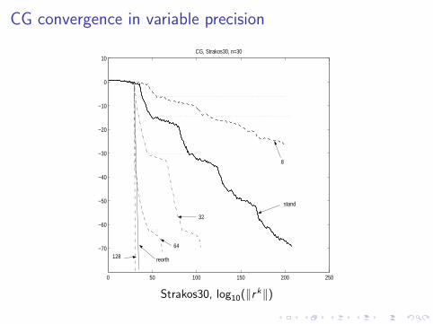
CG convergence in variable precision
0 50 100 150 200 250
−70
−60
−50
−40
−30
−20
−10
0
10CG, Strakos30, n=30
8
stand
32
64
128 reorth
Strakos30, log10(‖rk‖)
W.E. Arnoldi, The principle of minimized iterations in thesolution of the matrix eigenvalue problem, Quarterly of Appl.Math., v 9, (1951), pp 17–29
G.H. Golub and C. Van Loan, Matrix Computations,Third Edition, Johns Hopkins University Press, (1996)
G.H. Golub and R. Underwood, The block Lanczosmethod for computing eigenvalues, in Mathematical SoftwareIII, J. Rice Ed., (1977), pp 361–377
M.R. Hestenes and E. Stiefel, Methods of conjugategradients for solving linear systems, J. Nat. Bur. Stand., v 49n 6, (1952), pp 409–436
C. Lanczos, An iteration method for the solution of theeigenvalue problem of linear differential and integral operators,J. Res. Nat. Bur. Standards, v 45, (1950), pp 255–282
C. Lanczos, Solution of systems of linear equations byminimized iterations, J. Res. Nat. Bur. Standards, v 49,(1952), pp 33–53
G. Meurant, Computer solution of large linear systems,North–Holland, (1999)
G. Meurant, The Lanczos and Conjugate Gradientalgorithms, from theory to finite precision computations,SIAM, (2006)
G. Meurant and Z. Strakos, The Lanczos and conjugategradient algorithms in finite precision arithmetic, ActaNumerica, (2006)
C.C. Paige, The computation of eigenvalues andeigenvectors of very large sparse matrices, Ph.D. thesis,University of London, (1971)
Z. Strakos, On the real convergence rate of the conjugategradient method, Linear Alg. Appl., v 154–156, (1991),pp 535–549
![Model Order Reduction for Networked Control Systems...Model Order Reduction Iterative Rational Krylov Algorithm (IRKA) [ Gugercin et al. '08 ] Fixed-point iteration algorithm, based](https://static.fdocuments.net/doc/165x107/60b2c7a9c81c401954395c0c/model-order-reduction-for-networked-control-systems-model-order-reduction-iterative.jpg)